common_cause_failures - an analysis methodology and examples
DESCRIPTION
Common cause failueres - AnalysisTRANSCRIPT

1
Commoncausefailures.doc Enrico Zio, April 2002
Common Cause Failures An Analysis Methodology and examples
• FOREWORD
All modern technological systems are highly redundant but still fail because of common cause failures. The treatment of this kind of failures is still an open problem in PSA (Probabilistic Safety Assessment). Dependent failures are extremely important in risk quantification and must be given adequate treatment to avoid gross underestimation of risk

2
1. GENERAL CLASSIFICATION
Dependent failures may be classified in two main groups:
i. Common Cause Failures These are multiple failures which are a direct result of a common or shared root cause. The root cause may be extreme environmental conditions (fire, flood, earthquake, lightning, etc.), failure of a piece of hardware external to the system, or a human error. The root cause is not a failure of another component in the system. Operation and maintenance errors are often reported to be the root cause failures (carelessness, miscalibrations, erroneous procedures). We define ‘multiplicity’ of the common cause failure as the number of components that fail due to that common cause.
ii . Cascading failures These are multiple failures initiated by the failure of one component in the system (chain reaction or domino effect.) When several components share a common load, failure of one component may lead to increased load on the remaining ones and, thus, to an increased likelihood of failure.
One of the best-known accidents resulting from a common cause failure is the fire at Browns Ferry nuclear plant (Alabama, USA, 1975). Two operators used a candle to check for air leaks between the cable room and one of the reactor buildings, which was kept at a negative air pressure. The candle’s flame was sucked in along the conduct, and the methane seal, used where the cables penetrate the wall , caught fire. The fire went on to damage 2000 cables, including those of automatic Emergency Shutdown systems, and of all manually operated valves, except for four relief valves. With these four valves, it was possible to close down the reactor and avoid nuclear meltdown. As a feedback from the accident, the cables of the different ESDs were placed in separate conduits and no combustible filli ng (e.g. urethane foam) was used
2. IDENTIFICATION AND PROTECTION
To identify dependent failures, FMEA approaches must be extended to encompass potential interdependencies between the components, which may lead to common cause or cascading failures. In general, the most important defense against accidental component failures is the use of redundancy. The fire at Brown Ferry shows however, that redundancy itself is not enough, precisely because of dependent failures. Some general defensive strategies to avoid dependent failures are: - Barriers (physical impediments that tend to confine and/or restrict a potentially
damaging condition) - Personnel training (ensure that procedures are followed in all operation conditions) - Quali ty control (ensure the product is conforming with the design and that its operation
and maintenance follow the approved procedures and norms) - Redundancy - Preventive maintenance - Monitoring, testing and inspection (including dedicated tests performed on redundant
components following observed failures)

3
- Diversity (equipment diversity as for manufacturing, functional diversity as for the physical principle of operation)

4
3. DEFINITION OF DEPENDENT FAILURES
From a probabili stic point of view, two events A and B are said to be independent if: P (A,B)=P(A)· P(A|B) ≠ P(A) · P(B) We distinguish:
1. Common Cause initiating events (external events)
Events that have the potential for initiating a plant transient and increase the probabili ty of failure in multiple systems. These types of events require a full , dedicated risk analysis. e.g. fires, floods, earthquakes, loss of offsite power
2. Intersystem dependences
A. Functional dependences (from plant design): System 2 functions only if system 1 fails.
B. Shared-equipment dependences: Dependences of multiple systems on the same components, subsystems, or auxili ary components. E.g. components in different systems fed from the same electrical bus.
C. Physicals interactions: Failures of some system create extreme environmental stresses, which increase the probabili ty of multiple-system failures. E.g. failure of one system to provide cooling results I excessive temperature which cause the failure of a set of sensors.
D. Human-interaction dependences Dependences introduced by human actions, including errors of omission and commission. E.g. an operator turns off a system after faili ng to correctly diagnose the conditions of a plant (Emergency Core Cooling System, ECCS, in Three Mile Island).
3. Intercomponent dependences Events or failure causes that result in dependence among the probabiliti es of failure for multiple components or subsystems. The same cases A-D of intersystem dependences exist for intercomponent dependences as well .

5
4. METHODS FOR DEPENDENT-FAILURE ANALYSIS We can distinguish between
i EXPLICIT methods
Involve the identification and treatment of specific root causes of dependent failures at the system level, in the event-and fault-tree logic. Examples are earthquakes, fires and floods, which are treated explicitly as initiating events in the risk analysis.
ii IMPLICIT methods
Multiple failure events, for which no clear root cause event can be identified, can be modeled using implicit, parametric models. In the methods, new reliability parameters are added to the usual list to account for dependent failures.

6
4.1 EXAMPLES OF EXPLICIT METHODS
A. Functional dependences
System 2 is not needed (NN) unless system 1 fails
B. Shared-equipment
- Method of the “event trees with boundary conditions’’ To ill ustrate the event-tree approach for analyzing dependences of type 2.B., shared equipment, suppose that the fault trees developed for systems 1 and 2 are found to contain the same component failures, A and F, as primary events:
IE S1
NN α,β
γ
δ
Y
Y N
N
S2 Sequence

7
Components A and F have shared-equipment dependences and can be treated by incorporation into the event tree as follows: To complete the analysis, the system fault trees are quantified as conditional on the states of A and F, which are treated as “house “ events. For example, along sequences δ’ ’ the fault tree for system 1 is quantified with P(A)=1 and P(F) = 0, which gives the conditional minimal cut sets {C, B, DE}. On the other hand, along sequence δ the conditions are P(A)=0 and P(F)=0, which gives the minimal cut sets for system 1 of {C, DE}.
- Method of “Fault tree link” The fault trees of system 1 and 2 are linked together, thus developing a single large fault tree for each entire accident sequence. E.g. sequence γ: top event “S1 fails, S2 operates” ⇒ FT=FT1 @�)7 2 where FT1 is the fault tree of system 1 and FT2 the success tree for system 2.
Initiating event
Component A operates
Component F operates
System 1 operates
System 2 operates
α
β
γ
δ
α`
β`
δ``
δ```
IM IM
IM
IM
IM IM
IM = Impossible
Sequence

8
Figure 1 Hypothetical fault tree for sequence γγ. Here X denotes failure; X denotes the successful functioning of the component
The minimal cut sets can be found as follows:
{ }DEAFGCAFGmcs
GFAEDC
GFAFEDCBASS
;
)()]([
][])()[(21
=
∩∩∩∪∪=
∪∪∩∪∩∪∪∩=∩=γ
When rigorously followed, both FT-linking and event trees with boundary conditions correctly model the shared-equipment dependencies and both entail, apparently, the same level of data processing.

9
C. Physical Interactions
System 2 can operate only if system 1 operates successfully. When system 1 fails a physical interaction takes place, which inhibits system 2.
1. Intercomponent dependences (common-cause failures)
E.g. Three-component system
The corresponding system unavailability Q can be expressed as
Q=P(A AND B) + P(C) - P(A AND B AND C) Or alternatively as
Q=P(A) • P(B|A)[1-P(C|A AND B)] + P(C) for P(B|A)>> P(B) Any cause of failure that affects any pair, or all three, components at the same time will have an effect on the system unavailability.
IM N
N
Y Y
IE S1 S2
δ(γ=0)
α
β

10
Neglecting common-causes of failures (i.e. assuming component independent unavailabilities) leads to:
- Optimistic predictions of system reliability for components in the same mcs - Conservative predictions of system reliability for components in different mcs (i.e. in
series) The causes of single and multicomponent failures can be represented in the format of a fault tree where the causes appear at the level below the basic component-failure modes.
Figure 2 Fault tree for a three-component system with independent and common causes
D=common cause shared by redundant components A and B (∈ same mcs) E= common cause shared by components in series (≠mcs)
Minimal cut sets Without
Common Causes With
Common Causes A,B A` ,B C C`
D E

11
Example of quantification:
Fault-tree quantification case
A,B Parallel B,C series
Parameter Case 1
No common cause, no single
failures
Case 2 Common causes
A and B, no single failures
Case 3 No redundancy,
no common-cause failure
Case 4 No, redundancy,
common causes B and C
P(A’) 1.0 x 10⁻³ 9.9 x 10⁻⁴ 1 1 P(B’) 1.0 x 10⁻³ 9.9 x 10⁻⁴ 1.0 x 10⁻³ 5.0 x 10⁻⁴ P(C’) 0 0 1.0 x 10⁻³ 5.0 x 10⁻⁴ P(D) 0 1.0 x 10⁻⁵ 0 0 P(E) 0 0 5.0 x 10⁻⁴
Q 1.0 x 10⁻⁶ 1.1 x 10⁻⁵ 2.0 x 10⁻³ 1.5 x 10⁻³
4.2 AN EXAMPLE OF IMPLICIT METHODS FOR MODELLING DEPENDENT
FAILURES: THE WASH 1400 SQUARE ROOT METHOD
In many situations, a quantitative failure analysis based on the assumption of independence will l ead to unrealistic results. Thus, large efforts are being made to develop suitable models that take into account different types of dependence.
The square-root method In the reactor safety study, WASH 1400, a simple bounding technique was used to estimate the effect of common cause failures on a system. Let us consider a parallel system of two components A and B. The probabili ty that the system is down is P(A∩B). Since A∩B ⊆ A,
P(A∩B)≤P(A) (1) And similarly
Effects of a common cause shared by redundant components (i.e. ∈ same mcs). Component unavailabili ty is 1 E-3 in both cases. As the common-cause contribution P(0) is varied from 0 to 1%, the system unavailabili ty Q is increased by more then a factor of 10
Effects of a common cause shared by components in series (i.e. ∉ same mcs). Component unavailabili ty is 1 E –3 in both cases. As the common cause contribution P(E) increases from 0 to 5%, the system unavailabili ty decreases by 30%. Hence, this type of common cause can usually be ignored with a small error on the conservative side.

12
P(A∩B)≤P(B)
Hence,
P(A∩B)≤ min[P(A),P(B)] If A and B are independent,
P(A∩B)=P(A)P(B) Whereas, if they are positively dependent
P(A|B)≥P(A)
Thus,
P(A∩B)= P(A|B)P(B) ≥P(A)P(B) (2) Combining (1) and (2),
P(A)P(B) ≤ P(A∩B)≤ min[P(A),P(B)] In WASH-1400, P(A∩B) was then calculated as the geometric mean of PL and PU:
ULM PPBAP =∩ )(
There is, however, no proper theoretical foundation for the choice of the geometric average.
PL PU

13
Example Consider a parallel structure of n identical components, each with unavailability q at a specified time t. Let Ai denote the situation that component i is down at time t. Then, P(Ai)=q, i=1,2,…,n.
qAPAPAPPqAPP nU
n
i
niL ==== ∏
=
)](),...,(),(min[ )( 211
2
1+
==n
ULM qPPQ
n Independent components
(Q=qn) Square root method
2
1+
=n
M qQ
1 10-2 10-2
2 10-4 10-3 3 10-6 10-4 4 10-8 10-5 5 10-10 10-6
With q=10-2
14
5. A METHODOLOGICAL FRAMEWORK FOR COMMON CAUSE FAILURES ANALYSIS The treatment of common-cause failures (CCF) within a probabilistic safety assessment require four phases:
i. System logic model development
ii. Identification of common-cause component groups iii. Common-cause modeling and data analysis iv. System quantification and interpretation of results
5.1 SYSTEM LOGIC MODEL DEVELOPMENT
This phase consists of the following three steps:
5.1.1. System familiarization 5.1.2. Problem definition (root causes of common failures to be included in the analysis) 5.1.3. Logic model development
It is a fundamental step for any system analysis, but with respect to the usual analyses more emphasis is put on dependent failures. The aim of this phase is to identify and understand the physical and functional links in the system, functional dependences and interfaces and develop the corresponding logic models of the system (FT/ET).
5.2. IDENTIFICATION OF COMMON CAUSE COMPONENT GROUPS
The objectives of this phase are: - Identifying group of components to be included in the CCF analysis - Prioritizing the groups for the best resource allocation - Providing engineering arguments for data analysis and defense alternatives The end result of this stage is a definition of components for which common cause failures are to be included in the model, and determination of which root causes and coupling mechanisms should be included in the common cause events for the purpose of quantification. The following definition of common cause component group holds: DEFINITION: “A common cause component group is a group of similar or identical components
that have a significant likelihood of experiencing a common cause event’’. Qualitative and quantitative screenings are performed to separate the important component-cause groups, so as to keep the analysis to a manageable size.
5.2.1. Qualitative analysis
A search is made for common attributes and mechanisms of failure that can lead to potential common cause failures.

15
A useful check list of key attributes of similarity which can affect component interdependence , may be the following:
- Component type - Component use - Component manufacturer - Component internal conditions (pressure, temperature, chemistry) - Component boundaries and system interfaces - Component location name and/ or code - Component external environmental conditions (humidity, temperature, pressure) - Component initial conditions and operating characteristics (standby, operating) - Component testing procedures and characteristics - Component maintenance procedures and characteristics
Practical guidelines to the followed in the assignment of component groups are:
- Identical components used to provide redundancy should always be assigned to a common cause group
- When diverse redundant components have piece parts that are identically redundant, the components should not be assumed to be fully independent-
- Susceptibility of a group of components to CCF not only depends on their degree of similarity but also on the existence or lack of defensive measures( barriers) against CCF.
5.2.2. Quantitative screening
In performing quantitative screening for CCF candidates, one is actually performing a complete quantitative common cause analysis except that a conservative and very simple quantification model is used. The following steps are carried out:
5.2.2.1. The fault trees are modified to explicitly include a single CCF basic event for each component in a common cause group that fails all members of the group.
AI,BI,CI= independent failure events CABC=common cause failure event

16
5.2.2.2. Fault trees are solved to obtain the minimal cut sets. For each cut set {AI,BI,CI} there is also one including CABC (In the truncation the numerically larger probability CABC will survive while the joint event { AI,BI,CI } is often lost).
5.2.2.3. Numerical values for the CCF basic events can be estimated by the beta factor model (conservative regardless of the number of components in the CCF basic event):
P(CABC)=βP(A) β=0.1 for screening P(A)=total random failure frequency in absence
of common cause 5.2.2.4. Those common events, which are found to contribute little to the overall
system failure frequency are screened out. 5.3. COMMON CAUSE MODELLING AND DATA ANALYSIS The Objective of this phase is to complete the system quantification by incorporating the effects of common cause events for component groups that survive the screening process at stage 5.2. The following steps are carried out:
5.3.1. Definition of common cause basic events This step is equivalent to a redefinition of the logic model basic events to a lower level of detail that identifies the particular impacts that common cause events of specified multiplicity may have on the system:
⇒
Component level mcs: {A,B},{A,C},{B,C} S=A· B+A· C+B· C= (A ∩ B) ∪ (A ∩ C) ∪ (B ∩ C)
Common cause impact level (each component basic event becomes a sub tree) mcs={AI,BI},{AI,CI},{BI,CI},
{CAB},{CAC},{CBC},{CABC} (proliferation of cut sets) AT =AI+CAB+CAC+CABC S=AI· BI+AI· CI+BI· CI+CAB
+CAC+CBC+CABC

17
5.3.2. Selection of implicit probability models for common cause basic events
We can distinguish the different models into categories according to number of parameters: • single-parameter: beta factor model which produces conservative results for high
redundancy systems • multi -parameter: provide a more realistic assessment of CCF frequencies for
redundancy levels higher than two.
or into categories according to how multiple failures occur: • Shock models: the binomial failure rate model which assumes that the system is
subject to a common cause ‘shock’ at a certain rate. The common cause failure frequency is the product of the shock rate and the conditional probabili ty of failure, given a shock.
• Non-shock models Direct: use the probabiliti es of common events directly (Basic
parameter model) Indirect: estimate probabiliti es of common cause events through the
use of other parameters
Basic parameter model This model makes use of the rare events approximation
P(S)=P(AI)P(BI)+P(AI)P(CI)+ P(BI) P(CI)+P(CAB)+P(CAC)+P(CBC)+P(CABC)
under the following assumptions: 1. The probabili ty of similar events involving similar types of components are the same 2. Symmetry assumption: the probabili ty of failure of any given basic event within a common
cause component group depends only on the number and not on the specific components in that basic event
3221
321
3
2 33
2
)(
)()()(
)()()(
QQQQ
QQQQ
QCP
QCPCPCP
QCPBPAP
S
t
ABC
BCACAB
IIII
++=++=
====
===
Generalizing, the total failure probabili ty of a component in a common cause group of m components is:
K
m
kt Q
k
mQ ∑
=
−−
=1 1
1
Beta-factor model It models dependent failures of two types: intercomponent physical interactions (3C) and human interactions (3D).
(total probability of failure of a component)
(System) 2-out-of-3 logic
Ideally, the Qk values can be calculated from data. Unfortunately all the data are normally not available. Other models have been developed that put less stringent requirements on the data. This however is only done at the expense of making additional assumptions that address the incompleteness of the data.

18
The model assumes that Qt, the total probabili ty failure for each component, can be expanded into an independent, QI and a dependent, Qm contribution where m is the number of components in the common cause group (in other words, the common cause failure is such to fail all m components in the group). All Qk’s are then 0 except QI and Qm:
Qt=QI+Qm
A parameter β is defined as the fraction of the total failure probabili ty attributable to dependent failures:
ttStI
tm
mI
m
t
m QQQQQ
Q
Q
Q βββ
ββ +−=
−==
⇒+
== 22)1(3)1(
For system with more than two units, the beta-factor model does not provide a distinction between different numbers of multiple failures. Thus, simpli fication can lead to conservative predictions when it is assumed that all units fail when a common-cause failure occurs. The strength of the beta-factor model li es in its direct use of experience data and its flexibili ty. The total component failure probabili ty Qt and β must be estimated. For time distributions of failure probabiliti es
t
mt
t
t
m
t
m
e
e
Q
Q
λλβ λ
λ
≈−−== −
−
1
1
Example Consider a parallel structure of n identical and independent components with failure rate λ. An external event can cause simultaneous failure of all components in the system. Such event may be represented by a ‘hypothetical’ component C that is in series with the rest of the system. We assume the system to be non reparable and let RI(t) denote the survivor function of the identical components while RC(t) denotes the survivor functions of the hypothetical component C. Then, RC(t)=e−βλt and the survivor function for the system is
tnt
Cn
I
ee
tRtRtRβλλβ −−− ⋅−−=
⋅−−=
])1(1[
)(]))(1(1[)()1(
Exercise (Set n=4 and plot R(t) for various valves of β and t[0;2]) Note that, as expected, when the common cause factor β is increased, the reliabili ty of the system declines. Exercise Consider the three simple systems:
a) A single component b) A parallel structure of two identical components c) A 2-out-of-3 system with two identical components
System with 2-out-of-3 logic

19
All the components have the same constant failure rate λ. The systems are exposed to common cause failures, which we model through the β factor. Compute the survivor function and the MTTF. For λ=1, plot MTTF vs. β. Solution
a) For the single component, common cause failures are irrelevant
λλ 1
)( )()( == −a
ta MTTFetR
b)
λβλ
λβλ
λβλβλβ
)2(12
2
]2[ )(
)(
)2(
)1(2)1(2)(
−−=
−⋅=
⋅−⋅=−−−
−−−−−
b
tt
tttb
MTTF
ee
eeetR
c)
λβλβ
λβλβ
λβλβλβ
)23(
2
)2(
3
23
]23[ )(
)(
)23()2(
)1(3)1()(
−−
−=
⋅−⋅=
⋅⋅−⋅=−−−−
−−−−−
b
tt
tttc
MTTF
ee
eeetR
Obviously, all three systems have the same MTTF when β=1 (total dependence) Multiple Greek letters model The following equation allows to compute the probability of common cause failures of order k:
tk
k
iik Q
k
mQ )1(
1
11
11
+=
−
−−
= ∏ ρρ (m-1 parameters)
ρ1=1 ρ2=β= conditional probability of the failure of at least one additional component, given that one has
failed ρ3=γ= conditional probability of the failure of at least one additional component, given that two
have failed ρ4=δ= conditional probability of the failure of at least one additional component, given that three
have failed ................................................................................................ Example:

20
ttts
s
t
t
t
t
QQQQ
QQQQ
QQQQ
βγγββ
βγ
γβ
β+−+−=
++=
=
−=
−=++=
)1(2
3)1(3
32
)1(2
1
)1(
2
system 3-of-out-2 22
322
1
3
2
1
321

21
α-factor model The following equations hold:
∑=
=m
k
mk
mk
mk
Qk
m
Qk
m
1
)(
)(
)(α (m parameters)
11
)( =∑=
m
k
mkα normalization
tt
mkm
k Q
k
mk
Qα
α )()(
1
1
−−
=
∑=
=
=m
kkt kQ
mk
1
...2,1
α
Example m=3:
tt
tt
tt
S
tt
tt
tt
T
QQQ
QQQQ
αα
αα
αα
ααα
αα
ααααα
322
2
1
3221
)3(3)3(
3
)3(2)3(
2
)3(1)3(
1
)3(3
)3(2
)3(1
333
33
3
32
)3/2(
++
=
++=
=
=
=
++=
Binomial failure rate (BFR) model Consider a system composed of m identical components. Each component can fail at random times, independently of each other, with failure rate λ. Furthermore, a common cause shock can hit the system with occurrence rate µ. Whenever a shock occurs, each of the m individual components may fail with probabili ty p, independent of the states of the other components. The term ` binomial` failure rate is used because the number I of individual components faili ng as a consequence of the shock is thus binomially distributed with parameters m and p:
imi ppi
miIp −−
== )1(][ i=0,1,…,m
Two conditions are further assumed:
i. Shocks and individual failures occur independently of each other

22
ii. All failures are immediately discovered and repaired, with negligible repair time The assumption that the component will fail independently of each other, given that a shock has occurred, is often not satisfied in practice. The problem can, to some extent, be remedied by defining one fraction of the shocks as being ` lethal shocks` , namely shocks that automatically cause all the components to fail (p=2). If all the shocks are lethal, one is back to the β-factor model. Observe that the case p=1 corresponds to the situation that there is no built-in protection against these shocks. The BFR model differs from the beta-factor model in that it distinguishes between the numbers of multiple-unit failures in a system with more than two units:
−
+= −1
1 )1(1
mppm
m µλλ Failure rate of one unit
−
+= −imi
i ppi
mm )1(µλλ Failure rate of i units, i=2,...,m
Three parameters, λ, µ an p needs to be estimated.
Rate of single-unit failures from
common cause shocks
s
Total contribution due to independent
failures

23
5.3.3. Data classification and screening
The available data sources: generic raw data plant specific data generally classified event data parameter estimates.
In principle:
− A complete set of events should be found for each of the common cause
component groups.
− A complete set of events should be found for each of the common cause component groups.
In practice the classification of an event occurs as shown in Table 5.3.1 and 5.3.2:
Plant(Date) Status Event Description Cause-Effect Diagram
Maine Yankee
(August 1977) Power
Two diesel generators failed to run due to plugged radiator. The third unit radiator
was also plugged. (Uncertainty in the number of
components failed in the event)
Table 5.3.1 event classification
Component Group Size
Hypothesis Probability F0 F1 F2 F3 Shock type Fault Mode
I1 0.9 0 0 1 0 I2 0.1 0 0 0 1
Nonmetal Failure during
Operation P0 P1 P2 P3
3 Average
Impact Vector(I) 0 0 0.9 0.1
Table 5.3.2 Multiple hypothesis Impact Vector Assessment
As shown in Table 5.3.2, the impact Vector I of an event that has occurred in a component group of size m has m+1 elements, each representing the number of components that failed or could have failed in the event. If in an event k components fail, the kth element of the impact vector is 1 while all other elements are zero. A condensed representation of the binary impact vector is:
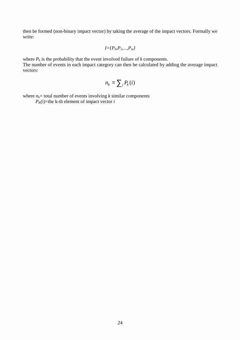
I={I0,I1,...,Im} In many reports the description of the event is not clear so that the classification of the event may require several hypotheses I1,I2,…(different interpretations of the event) each with a probability representing the analyst’s degree of confidence in that hypothesis. An average impact vector can
24
then be formed (non-binary impact vector) by taking the average of the impact vectors. Formally we write:
I={P0,P1,...,Pm} where Pk is the probability that the event involved failure of k components. The number of events in each impact category can then be calculated by adding the average impact vectors:
∑=i kk iPn )(
where nk= total number of events involving k similar components
PK(i)=the k-th element of impact vector i

25
5.3.4. Parameter Estimation
The purpose of this step is to use the pseudo-data generated in the previous step to provide estimates of either the basic event probabiliti es directly (using the basic parameter model) or the parameters of the common cause failure models (beta, BFR, etc.). The information provided by the set of impact vectors is the number of events in which 1,2,3,....m components failed (m=level of redundancy)
Example Beta-factor estimation for a two-train redundant standby safety system tested for failures:
(unknown) causecommon for test of n.evidence
ˆˆ
2
2 ==N
nβ
We also have
2
21
2
2
21
22
N
n
N
nN
n
Q
Q
Q
t +=
+==β
The available evidence is: n1 failures of single components
n2 failures of both components The unknowns are: N, number of single-component demands to start
N2, number of tests for single common-cause failures The fundamental assumption is that an estimate of the total single component failure probabili ty Qt exists. The unknown number N of single-component demands to start can be estimated from:
tt Q
nnN
N
nnQ 2121 22 +=⇒+=
The other unknown N, number of effective tests for common cause failures, depends on the surveill ance testing strategy:
S1: Both components are tested at the same time. Then,
⇒N2=2
N
⇒2/
22 N
nQ =
⇒21
2
2
21
2
2
2
2
2/
2/nn
n
N
n
N
nN
n
Q
Q
t +=
+==β

26
S2: The components are tested at staggered intervals, one every two weeks, and if there is a failure, the second component is tested immediately. In this case, the number of tests against the common cause is higher because each successful test of a component is a confirmation of the absence of the common cause:
⇒N=N2+n1+n2
Then,
N
n
N
nQ 2
2
22 ≈= (n1 and n2 << N) (
2
1≈ of S1)
21
2
21
2
2
nn
n
N
nnN
n
Q
Q
t +=+==β
Estimates of β are therefore based on particular assumptions on the testing strategies.
Successful test 1 fails 2 fails
These arise because of the failure of the first component, which occurs n1 times on its own and n2 times in conjunction.

27
Binomial failure rate estimation We need to estimate p and µ The shock rate µ is not directly available from the data because:
1. Shocks that do not cause any failure are not observable 2. Single failures from common-cause shocks may not be distinguishable from single
independent failures. We define the rate of dependent multiple failures (any)
[ ]1
2
)1()1(1 −
=+ −−−−== ∑ mm
m
ii pmppµλλ
(*)
With Ni=number of observations of i concurrent failures
N+=∑=
m
iiN
2
= number of observations of multiple failures of any order
We estimate the parameters p, µ, λ1 by maximizing the likelihood of the observed data:
[ ] [ ] [ ] [ ]mmmmmT nNnNPnNPnNPnNnNnNP ==⋅=⋅====== +++ ,...,..., 221112211 (**) Now, the variables N1 and N+ have Poisson distributions with parameters λ1T and λ+T, respectively (T=system operating time). Maximizing the likelihoods P1 and P+ in (**) we get, respectively:
T
n11 =λ ;
T
n++ =λ
The third factor Pm follows a multinomial distribution and the estimate of p, which maximizes Pm, is found from:
( )[ ]( ) ( ) 1
1
111
11−
−+
−−−−−−=
mm
m
pmpp
ppmnS
Where ∑=
⋅=m
iiniS
2
is the total number of units failing in multiple-failure occurrences.
For example for m=3,
( )+
+
−−=
nS
nSp
32
23
With λ1, λ+ and p, we can find an estimate of µ from (∗).

28
Example: PWR Auxiliary Feedwater System (AFWS)
Instances of multiple failures in PWR auxiliary feedwater systems NE=11 multiple failure events for a total of Nc=24 unit failures
Number of trains
Plant Date Number of failure and
failed train type M T D Calvert Cliffs Unit 1 5/76 2/T,T 0 2 0 Haddam Neck 7/76 2/T,T 0 2 0 Kewaunee Unit 1 8/74
10/75 11/75
2/M,M 2/M,T
3/M,M,T
2 2 2
1 1 1
0 0 0
Point Beach Unit 1 4/74 2/M,M 2 1 0 Robert F. Ginna 12/73 2/M,M 2 1 0 Trojan Unit 1/76
12/77 2/T,D 2/T,D
0 0
1 1
1 1
Turkey Point Unit 3 5/74 3/T,T,T 0 3 0 Turkey Point Unit 4 6/73 2/T,T 0 3 0
Summary of PWR auxiliary feedwater experience Summation of number of systems times length of service
1874 system-months
Contribution to above by multiple-unit systems 1641 system-months Summation of number of units times length of service 4682 unit-months Contribution to above by multiple-unit systems 4449 unit-months Total number of single failures 69 Number of single failures in multiple-unit systems 68,Ni Number of multiple-unit failure events 11,Ne Number of unit failures in dependent-failure occurrences
24,Nc
Consider each train of the system as a unit. All of the incidents can be interpreted as unit failures to start.
29
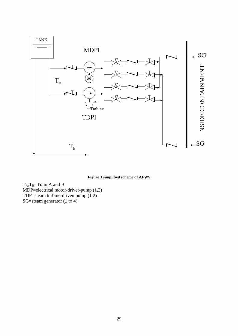
Figure 3 simplified scheme of AFWS
TA,TB=Train A and B MDP=electrical motor-driver-pump (1,2) TDP=steam turbine-driven pump (1,2) SG=steam generator (1 to 4)

30
Beta-factor model:
TT
T
q
Q
im
m
t
m
λλλ
β+
≅=ˆ
26.06824
24
32
32
//
/ˆ321
32 =+
=++
+=+
=+
=nnn
nn
TNTN
TN
ic
c
im
m
λλλβ
(The number of occurrences of multiple-unit failures, Ne, should not be confused with Nc in
determining β . A common error is to substitute Ne for Nc). Assuming one complete (i.e., all units) system demand for each calendar month, the per-demand probability of failure-to-start for a 1-out-of-2 system is:
tottot
tts
t
t
QQUQ
QU
QUβλλβββ
ββ
+−=
+−==⇒
=−= −
22
2221
2
1
)1(
)1(
)1(
For the estimates of the total failure rate we have:
02.04682
2468
)(1
32unit single a of demandon failure ofy probabilit 321 =+=
≡⋅+
=++
==NT
NN
N
nnn citotλ
so that the per-demand probability of failure-to-start for the 1-out-of-2 system is:
334221 104.5102.5102)02.0)(026.0()]02.0)(26.01[( −−−
− ⋅=⋅+⋅=+−=U
Note that data from both two- and three-unit systems were used to obtain a failure probability estimate for a two-unit system. For a 1-out-of-3-unit system, the contribution from multiple independent failures is negligible, so that the probability of failure to start is:
tottotU βλλβ )1( 3331 +−=− =5.2 10-3
The failure probabilities of 1-out-of-2 and 1-out-of-3 systems could also be estimated directly as follows:
System per-demand failure probability = 3107.3
operation of
months system 1641failures system 6 −⋅=
(1-out-of-2) Two-component per-demand failure prob. = 3104.8
operation of
months system -2 474
failures system 4 −⋅=
multiple indipendent failures
common cause failures

31
(1-out-of 3) Three-component per-demand failure probabili ty = 3107.1 4741641
failures system 2 −⋅=−
These estimates are inherently less robust. Note that the beta–factor method gives a comparatively higher failure probabili ty for 3-unit systems and a slightly lower probabili ty for 2-unit systems than the values calculated directly from data. Binomial failure-rate model As before, the equation in terms of failure rates λ are converted to failure-to-start probabiliti es assuming one system demand per calendar month.
0414.01641
68
11
1 ==⋅
=T
NU where N1 is the number of observations of single failures
0067.01641
11
12 ==⋅
=T
NU t where Nt is the number of observations of multiple failures of any order
Only data from the 7 three-unit systems can be used as evidence for the parameter p (three components group). The total number of units faili ng in the 7 multiple-failure occurrences in three-unit systems, S, is 16 for this example. Thus,
55.073162)7216(3
32)2(3
ˆ =⋅−⋅
⋅−=−−=
+
+
nS
nSp
45.0ˆ1 =− p
Then, the per-demand common-cause failure shock rate is estimated from
[ ]∑=
−+ −−−−==
m
i
mmi pmpp
2
1)1()1(1µλλ
0118.0ˆ
])45.0)(55.0(3)45.0(1[0067.0 23
=−−=
µµ
Using these estimators in
])1([ 1−−
= mi
i ppi
mµλ
the per-demand system failure probabiliti es for two of three units faili ng is
323221 108.4)45(.)55(.
2
3)0118.0( −−
− ⋅=
=U
and for three out of three units faili ng:
333231 109.1)45(.)55(.
3
3)0118.0( −−
− ⋅=
=U
32
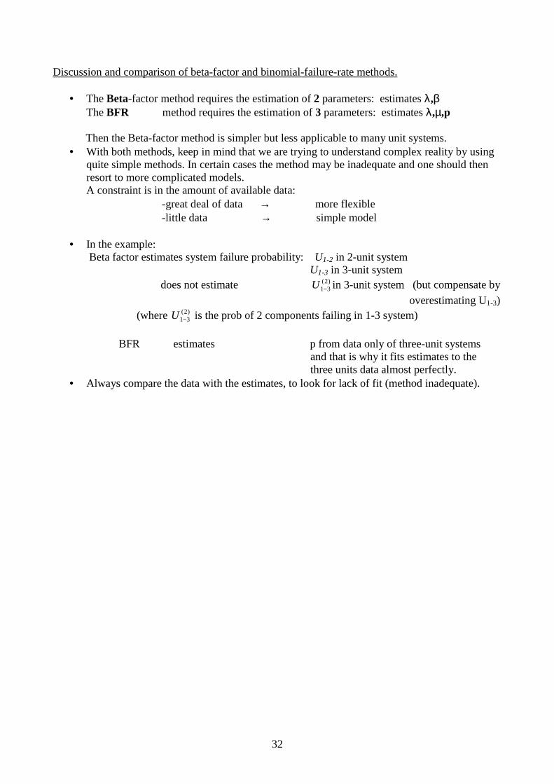
Discussion and comparison of beta-factor and binomial-failure-rate methods.
• The Beta-factor method requires the estimation of 2 parameters: estimates λλ,ββ The BFR method requires the estimation of 3 parameters: estimates λλ,µµ,p Then the Beta-factor method is simpler but less applicable to many unit systems.
• With both methods, keep in mind that we are trying to understand complex reality by using quite simple methods. In certain cases the method may be inadequate and one should then resort to more complicated models. A constraint is in the amount of available data: -great deal of data → more flexible -little data → simple model
• In the example: Beta factor estimates system failure probability: U1-2 in 2-unit system U1-3 in 3-unit system
does not estimate )2(31−U in 3-unit system (but compensate by
overestimating U1-3) (where )2(
31−U is the prob of 2 components failing in 1-3 system)
BFR estimates p from data only of three-unit systems
and that is why it fits estimates to the three units data almost perfectly.
• Always compare the data with the estimates, to look for lack of fit (method inadequate).