Common Lab Procedures used by the Marshall

Research Group

This manual presents methods and procedures commonly used in our lab group at UCSF involving some basic background on dental structures, sterilization, specimen preparation and storage techniques, as well as common testing procedures for atomic force microscopy, AFM based nanoindenation and basic mechanical testing. This should be useful in training for faculty, students, staff and visiting scholars and forms the basis of standardizing procedures in our studies of calcified tissues and biomaterials.

Kuniko Saeki, DDS, PhD, DDS Adjunct Assistant Professor Division of Biomaterials and Bioengineering UCSF Dept. of Preventive and Restorative Dental Sciences. September, 2010

Marshall Lab manuals contents

• Basics

1. Dental anatomy (Power Point)

Ø Tooth development schedule

2. Sterilization

Ø Storage of specimen

Ø Buffers (HBSS recipe)

Ø Various buffers, simulated body fluid recipes

ü Dulbecco’s PBS

ü GSK artificial saliva

ü Potassium phosphate buffer, sodium phosphate buffer, Tris buffer

Ø List of protease inhibitors

• AFM

1. Competency check list for AFM and hystiron

2. Hardware

Ø Cable connection guide

3. Reference layer techniques

4. AFM height analysis - precautions

5. Acid etching- kinetics study by AFM

Ø Z measurement)

6. Nano indentation

Ø Triboscope version 5

ü Appendix C: How to do new area functions

• 4 point bending instructions

Ø ELF instruction

Ø How to obtain flexural strength and modulus (digital attachment of excel macro

files)

• Digital image processing

1. What is appropriate in image processing

2. Image analysis with SCION image

Ø Examples. (dentin scallop analysis, EDX particle analysis)

• Templates and forms available

1. AFM data kinetics analysis.xls - Excel sheet for z measurement study

2. 4point macro book.xls - macro for 4 point bending data

• Hardware manuals

1. Mettler Balance AE240

2. pH meter

• Lab safety

1. Glove selection guide

9/23/2010

1

How many teeth do we have?

• Permanent teeth– Incisors– Canines– Premolars– Molars

• Deciduous teeth– Incisors– Canines– Molars

Terms for direction

• Mesial• Distal• Lingual • Buccal

• Coronal (occlusal)• Apical (cervical,gingival)

• Maxilla• Mandibula

mesiallabial

buccal

distal

palatal

lingual

1) Anatomical planes– Horizontal– Frontal – Sagittal

2) For the teeth– Occulusal– Bucco-lingual– Mesio-distal

plane

Median plane

horizontal plane

frontal planesagittal plane

Occlusal

Buccolingual(B-L)Mesio-distal (M-D)

Name the parts of the tooth

CrownRoot

Cusp

Ridge

Groove Pit

Cusp tip

Buccal/lingual?mesial or distal ??

• Functional cusps (molars)– Flatter– Upper: Lingual(palatal)– Lower:Buccal

• Buccal view and occlusal view– Line angle of mesial is

sharper than distal– Exception: upper 1st premolar

Incisor Canine Molar

Buccal

mesial

mesial

Traits of the teeth

• Incisors– Look like a scoop– Flat edge– Usually one root

• Canines– Triangular shape

crown– Usually one root

BuccalBuccal

upper lower

upper lower

9/23/2010

2

Traits of the teeth

• Premolars– Upper

Two cuspsOvoid shape crownTwo roots (1st pre)One root (2nd pre)

– LowerTwo cuspsSquare/round shape crownOne root

Upper 1st premolar

Lower 1st premolarOcc of 2nd

Buccal

Buccal

Traits of the teeth

• Molars– Upper

Square/ diamond-ish shape occl. surface

4 or 3 cusps3 root (2 buccal 1 palatal)

– LowerTrapoziod/ rectangle shape

occl. surface5 or 4 cusps2 root (mesial and distal)

Upper 1st molar

Lower 1st molarBuccal Distal

Buccal Mesial

3rd Molars

• A lot of variations• Less characters/traits• Less number of roots

upper

lower

If you slice it….Enamel

Dentin

DEJ

CEJ

• Supporting tissues• Cementum

– Acellular– Cellular

• Periodontal ligament(PDL)– Fibers in different orientations– Sensory system

• Alveolar Bone (socket)

CDJ

Enamel

• Hardest tissue in your body

• Highly mineralised– 96% inorganic

(apatite)• Enamel rods

enamel rods A: deciduous, B: permanent

Orientation of enamel crystal

Dentin– Inorganic 70% (hydroxyapatite)– Water 10%– Organic 20%

• Collagen 91% (most type I,+some V)

– Protein• Phosphoproteins, proteoglycans etc.

• Dentin tubules – occupy 20-30% of dentin– diameter 0.5-3μm– orientation

• Secondary dentin• Reparative dentin• Altered dentin

– Sclerotic dentin– Transparent dentin

9/23/2010

3

Pulp• Living tissue in the

tooth• Can make dentin

through the life• Sensory system

Tooth development

Diagrammatic representation of A, the bud, B, the cap, and, C, the bell stages of tooth development

Tooth development

• Bell stage of tooth development showing the outer enamel epithelium (OEE), stellate reticulum (SR), inner enamel epithelium (IEE) dental papila (DP) cervical loop (CL) successional lamina (SL) and dental sac (DS)

References• Stedman’s medical dictionary 26th Edition• Dorland’s medical dictionary 28th Edition• Orban’s oral histology and embryology (S.Bhaskar)9th Edition • Pathways of the pulp (S. Cohen, R Burns) 7th Edition• Dental Anatomy (M.Saheki)

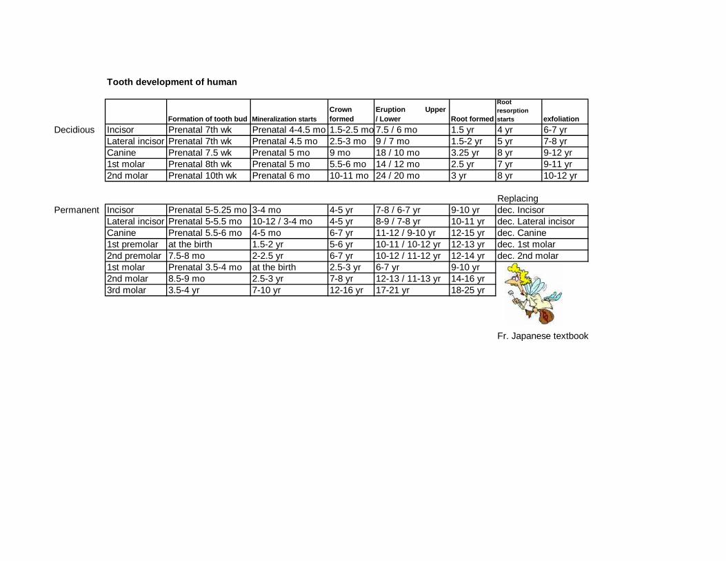
Tooth development of human

Formation of tooth bud Mineralization startsCrownformed

Eruption Upper/ Lower Root formed

Rootresorptionstarts exfoliation

Decidious Incisor Prenatal 7th wk Prenatal 4-4.5 mo 1.5-2.5 mo 7.5 / 6 mo 1.5 yr 4 yr 6-7 yrLateral incisor Prenatal 7th wk Prenatal 4.5 mo 2.5-3 mo 9 / 7 mo 1.5-2 yr 5 yr 7-8 yrCanine Prenatal 7.5 wk Prenatal 5 mo 9 mo 18 / 10 mo 3.25 yr 8 yr 9-12 yr1st molar Prenatal 8th wk Prenatal 5 mo 5.5-6 mo 14 / 12 mo 2.5 yr 7 yr 9-11 yr2nd molar Prenatal 10th wk Prenatal 6 mo 10-11 mo 24 / 20 mo 3 yr 8 yr 10-12 yr

ReplacingPermanent Incisor Prenatal 5-5.25 mo 3-4 mo 4-5 yr 7-8 / 6-7 yr 9-10 yr

Lateral incisor Prenatal 5-5.5 mo 10-12 / 3-4 mo 4-5 yr 8-9 / 7-8 yr 10-11 yrCanine Prenatal 5.5-6 mo 4-5 mo 6-7 yr 11-12 / 9-10 yr 12-15 yr1st premolar at the birth 1.5-2 yr 5-6 yr 10-11 / 10-12 yr 12-13 yr2nd premolar 7.5-8 mo 2-2.5 yr 6-7 yr 10-12 / 11-12 yr 12-14 yr1st molar Prenatal 3.5-4 mo at the birth 2.5-3 yr 6-7 yr 9-10 yr2nd molar 8.5-9 mo 2.5-3 yr 7-8 yr 12-13 / 11-13 yr 14-16 yr3rd molar 3.5-4 yr 7-10 yr 12-16 yr 17-21 yr 18-25 yr

Fr. Japanese textbook

dec. 2nd molar

dec. Incisordec. Lateral incisordec. Caninedec. 1st molar

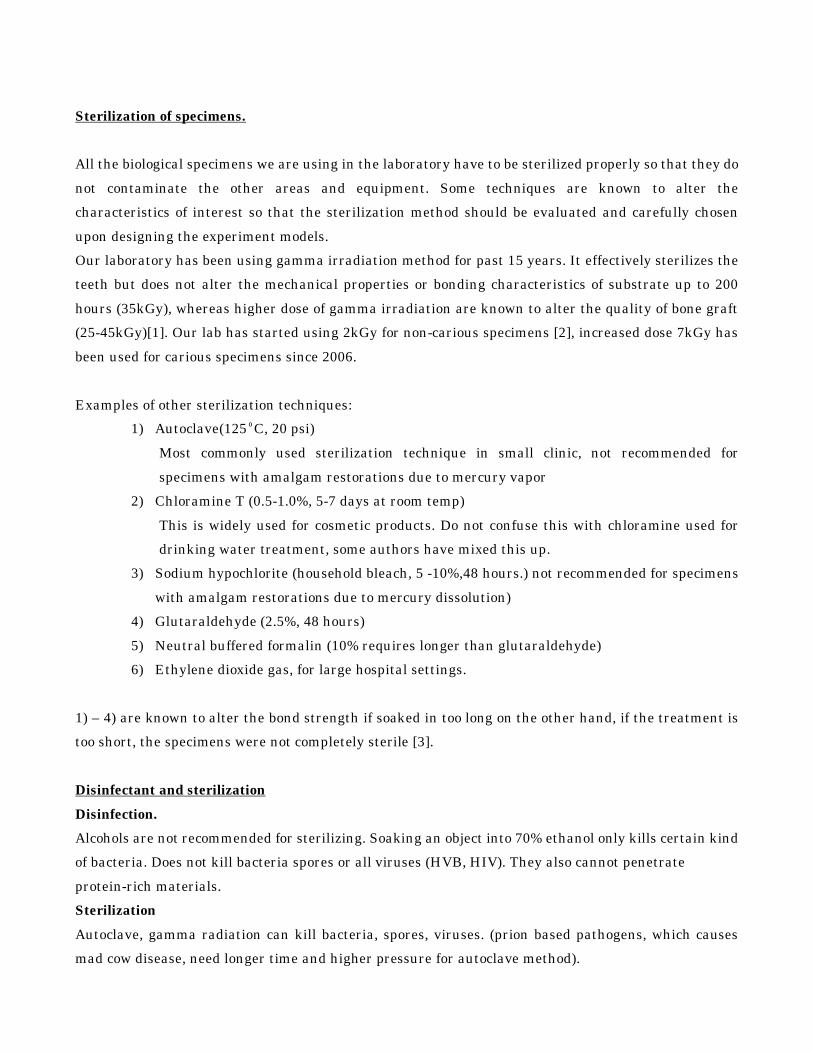
Sterilization of specimens. All the biological specimens we are using in the laboratory have to be sterilized properly so that they do not contaminate the other areas and equipment. Some techniques are known to alter the characteristics of interest so that the sterilization method should be evaluated and carefully chosen upon designing the experiment models. Our laboratory has been using gamma irradiation method for past 15 years. It effectively sterilizes the teeth but does not alter the mechanical properties or bonding characteristics of substrate up to 200 hours (35kGy), whereas higher dose of gamma irradiation are known to alter the quality of bone graft (25-45kGy)[1]. Our lab has started using 2kGy for non-carious specimens [2], increased dose 7kGy has been used for carious specimens since 2006. Examples of other sterilization techniques:

1) Autoclave(125ºC, 20 psi) Most commonly used sterilization technique in small clinic, not recommended for specimens with amalgam restorations due to mercury vapor

2) Chloramine T (0.5-1.0%, 5-7 days at room temp) This is widely used for cosmetic products. Do not confuse this with chloramine used for drinking water treatment, some authors have mixed this up.

3) Sodium hypochlorite (household bleach, 5 -10%,48 hours.) not recommended for specimens with amalgam restorations due to mercury dissolution)

4) Glutaraldehyde (2.5%, 48 hours) 5) Neutral buffered formalin (10% requires longer than glutaraldehyde) 6) Ethylene dioxide gas, for large hospital settings.

1) – 4) are known to alter the bond strength if soaked in too long on the other hand, if the treatment is too short, the specimens were not completely sterile [3]. Disinfectant and sterilization Disinfection. Alcohols are not recommended for sterilizing. Soaking an object into 70% ethanol only kills certain kind of bacteria. Does not kill bacteria spores or all viruses (HVB, HIV). They also cannot penetrate protein-rich materials. Sterilization Autoclave, gamma radiation can kill bacteria, spores, viruses. (prion based pathogens, which causes mad cow disease, need longer time and higher pressure for autoclave method).

When the experimental protocol calls for incubation, to suppress the bacterial growth we use supplemental method, mostly added to the solution.

1. thymol (0.5%) 2. chloramine T (0.5 to 1 % was used by Pashley’s group). 3. sodium azide (0.002% - 0.05%)

Storage of the specimens Biological specimens need to be stored properly to maintain their natural properties. We use mostly mineralized tissue, tooth, enamel, dentin, cementum and bone. The factors to consider is the hydration, ion balance and bacterial contamination so that unneeded alteration does not occur while we keep the specimen. Teeth specimens were collected in either distilled water (DI) or modified Hank’s balanced salt solution (HBSS). They were gamma radiated in the solution and stored at 4ºC until provided for your experiments. We recommend storing the specimens soaked in HBSS or sealed at 100% moisture on the DI wetted tissue stored at 4ºC. Storing dentin in DI water slowly demineralizes the exposed surface and alters the mechanical property [4]. Polished normal dentin specimens should be stored in HBSS and refrigerated. If the specimen is evaluated under AFM – nano mechanical properties, it is highly recommended to re-polish the surface with final 2 steps of diamond polishing paste to get fresh surface and minimize the effect of storage solution. If your specimen has demineralized or remineralized zone of interest, you may need to choose to store it dry or moist. If the demineralized specimen is totally desiccated, it needs more than 30 seconds to be reconstructed for the wet measurement. (we know in 24hours it was fully hydrated [5]. We usually aim for 2 hours (have not done comprehensive studies… ). Carefully choose the solution so that the ions in it will not alter the properties of your specimen.

Buffers Commonly used simulated body fluids are Ringer’s solution, Hank’s balanced salt solution(HBSS), PBS, Dulbecco’s PBS (+ with calcium and magnesium and – without them). For simulated oral environment, we sometimes use artificial saliva formula, too. The example of salts concentrations for simulated body fluids are shown below.

Blood plasmaRinger'ssolution SBF

NaturalSal iva

ArtificialSaliva

HanksBSS

DulbeccoPBS (-)

DulbeccoPBS (+) PBS mmol/L

1 Na+ 142.0 39.1 142.0 18.0 14.0 141.7 153.1 153.1 165.0

2 K+ 3.6-5.5 1.4 5.0 27.0 21.0 5.9 4.2 4.2 1.1

3 Mg2+ 1.0 0.0 1.5 0.8 0.5

4 Ca2+ 2.1-2.6 0.4 2.5 1.3 1.8 1.3 0.9

5 Cl- 95.0-107 40.7 148.8 20.0 30.0 144.9 139.6 142.3 154.0

6 HCO3- 27.0 0.6 4.2 4.2

7 HPO42-

0.65-1.45 0.0 1.0 4.5 4.7 1.2 9.6 9.6 6.7

8 SO42-

1.0 0.0 0.5 0.8

Reference Kokubo, 2004 SusTechHelebrant,2002 Mediatech

We mostly use HBSS but removed glucose from the original formula to suppress bacterial growth. It can be made with or without sodium azide. Phenol red is added as a pH indicator.

Hanks BSS(w/Ca Mg)

Modified for Marshall Lab, no glucose with phenol red and sodium azide

DI Water 1000 ml 4000 ml

1 NaCl sodium chloride 8 g 32 g

2 KH2PO4 potassium phosphate monobasic 0.06 g 0.24 g

3 KCl potassium chloride 0.4 g 1.6 g

4 MgSO4 .7H2O magnesium sulfate heptahydrate 0.2 g 0.8 g

5 CaCl2.2H2O calcium chloride dihydrate 0.185 g 0.74 g

6 Na2HPO4 sodium phosphate dibasic 0.0477 g 0.1908 g

7 d-glucose Dextrose 0 g 0 g

8 NaHCO3 sodium bicarbonate 0.35 g 1.4 g

9 Phenol red, Na Phenolsulfonephthalein Sodium salt 0.01 g 0.04 g

10 NaN3 sodium azide 0.02 %

How to make 4L of Hanks BSS

1) Measure 4L of DI water in a tank 2) Take 300-400ml of DI water from the tank into Flask 3) Measure and add 7 chemicals except CaCl2·2H2O into the flask, mix well 4) Take another 300-400 ml of DI water from the tank, dissolve CaCl2·2H2O 5) Transfer the solution into the tank, shake well 6) Rinse the flask with the solution from the tank several times. 7) Then add CaCl2 solution to the tank, mix well 8) Rinse the flask with the solution from the tank several times. 9) Add sodium azide and phenol red as needed 10) pH should be 7.1-7.4, if not, use 7.5% NaHCO3 to adjust pH.

pH ranges of selected Biological Buffers (0.1M, 25ºC)

pKa(at 25ºC) Useful pH Range

MES 6.10 5.5-6.7Bis-Tris 6.50 5.8-7.2ACES 6.73 6.1-7.5PIPES 6.76 6.1-7.5BES 7.09 6.4-7.8MOPS 7.20 6.5-7.9TES 7.40 6.8-8.2HEPES 7.48 6.8-8.2Tris 8.06 7.0-9.0Tricine 8.05 7.4-8.8Glycylglycine 8.20 7.5-8.9TAPS 8.40 7.7-9.1CHES 9.30 8.6-10.0CAPS 10.40 9.7-11.1

From Fisher catalog

Appendix Various buffers

FWArtificialSaliva Hanks BSS

DulbeccoPBS (-)

DulbeccoPBS (+) PBS

DI Water 1000 1000 1000 1000 1000 ml

1 NaCl sodium chloride 58.44 8 8 8 9 g

2 KH2PO4 potassium phosphate monobasic 136.1 0.54 0.06 0.2 0.2 0.144 g

3 KCl potassium chloride 74.55 2.24 0.4 0.2 0.2 - g

4 MgSO4 .7H2O magnesium sulfate heptahydrate 246.5(120.4) 0 0.2 - - -

5 MgCl2 .6H2O magnesium chloride 203.3(95.21) 0.04 - 0.1 - g

6 CaCl2.2H2O calcium chloride dihydrate 147.0(111.0) 0 - - - -

7 CaCl2 calcium chloride anhydrous 111 0.08 0.14 - 0.1 - g

8 Na2HPO4 sodium phosphate dibasic 142 0 0.0477 1.15 0 0.795 g

9 Na2HPO4.7H2O sodium phosphate dibasic heptahydrate 0 - 2.1716 -

10 NaN3 sodium azide 65.01 0.02

11 d-glucose Dextrose 180.2 0 1 0 0 - g

12 Phenol red, Na Phenolsulfonephthalein Sodium salt 376.36 0 0.01

13 HEPES buffer N-(2-hydroxyl)piperazine-N'-(2-etanesulfonic acid); 4-(2-Hydroxyethyl)piperazine-1-ethanesulfonic acid238.3 4.77

14 NaHCO3 sodium bicarbonate 84.01 0 0.35 0 0 - g

pH (before adjustment) 7.1 7.4±0.1 7.0±0.1 7.4±0.1

pH (final) 7.1-7.4Osmolality(mOsm) 275±15 276±10 276±12 287±15

Various Hanks BBS recipe

Japanesebiochem Mediatech

w/Mg, Ca w/o Mg, Ca

DI Water 1000 1000 1000 1000 ml

1 NaCl sodium chloride 8 8 8 8 g

2 KH2PO4 potassium phosphate monobasic 0.06 0.06 0.06 0.06 g

3 KCl potassium chloride 0.4 0.4 0.4 0.4 g

4 MgSO4 .7H magnesium sulfate heptahydrate ? 0 0.2 0.2 g

5 CaCl2 calcium chloride ? 0 0.14 0.14 g

6 Na2HPO4 sodium phosphate 0.09(7H2O) 0.09(7H2O) 0.12(12H2O) 0.0477 g

7 d-glucose Dextrose 1 1 1 1 g

8 NaHCO3 sodium bicarbonate 0.35 0.35 1 0.35 g

cost $12/L $2.4/L

We adapted Mediatech recipe

UCSF

Dulbecco PBS (w/Ca Mg)

DI Water 1000 ml 4000 ml

1 NaCl sodium chloride 8 g 32 g

2 KH2PO4 potassium phosphate monobasic 0.2 g 0.8 g

3 KCl potassium chloride 0.2 g 0.8 g

4 MgCl2 .6H2O magnesium chloride 0.1 g 0.4 g

5 CaCl2 calcium chloride anhydrous 0.1 g 0.4 g

6 Na2HPO4 sodium phosphate dibasic 0 g 0 g

7 Na2HPO4.7H2O 2.1716 8.6864 g

7 d-glucose Dextrose 0 g 0 g

8 NaHCO3 sodium bicarbonate 0 g 0 g

pH 7.0±0.1

GSK artificial saliva recipe from Dr. Parkinson (2009-2010) For 1 liter of DI water 50mM NaCl (2.92g/L) 1.1mM CaCl2·2H2O (0.16g/L) 0.6mM KH2PO4 (0.08g/L) Protein plus recipe, add 0.1% bovine serum albumine (1g/L) 0.1% porcine stomach mucin (1g/L) pH=7.0 0.05% sodium azide (0.5g/L)

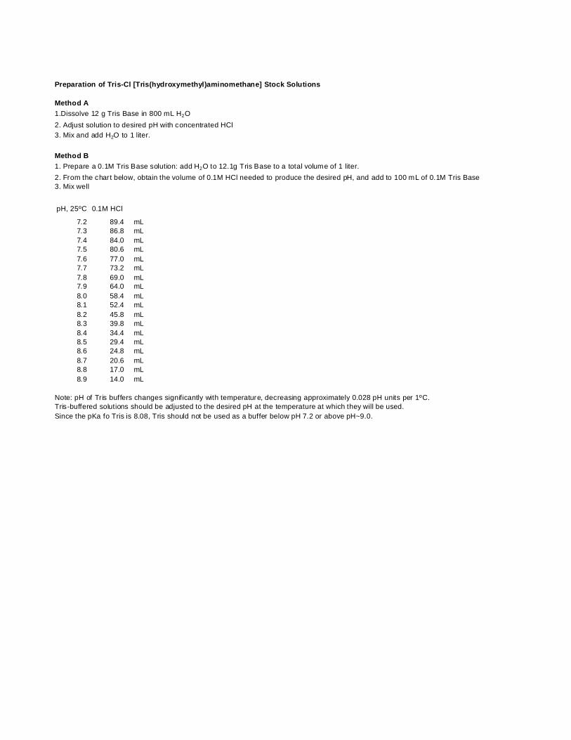
Preparation of Tris-Cl [Tris(hydroxymethyl)aminomethane] Stock Solutions

Method A1.Dissolve 12 g Tris Base in 800 mL H2O2. Adjust solution to desired pH with concentrated HCl3. Mix and add H2O to 1 liter.

Method B1. Prepare a 0.1M Tris Base solution: add H2O to 12.1g Tris Base to a total volume of 1 liter.2. From the chart below, obtain the volume of 0.1M HCl needed to produce the desired pH, and add to 100 mL of 0.1M Tris Base3. Mix well

pH, 25ºC 0.1M HCl

7.2 89.4 mL7.3 86.8 mL7.4 84.0 mL7.5 80.6 mL7.6 77.0 mL7.7 73.2 mL7.8 69.0 mL7.9 64.0 mL8.0 58.4 mL8.1 52.4 mL8.2 45.8 mL8.3 39.8 mL8.4 34.4 mL8.5 29.4 mL8.6 24.8 mL8.7 20.6 mL8.8 17.0 mL8.9 14.0 mL

Note: pH of Tris buffers changes significantly with temperature, decreasing approximately 0.028 pH units per 1ºC.Tris-buffered solutions should be adjusted to the desired pH at the temperature at which they will be used.Since the pKa fo Tris is 8.08, Tris should not be used as a buffer below pH 7.2 or above pH~9.0.

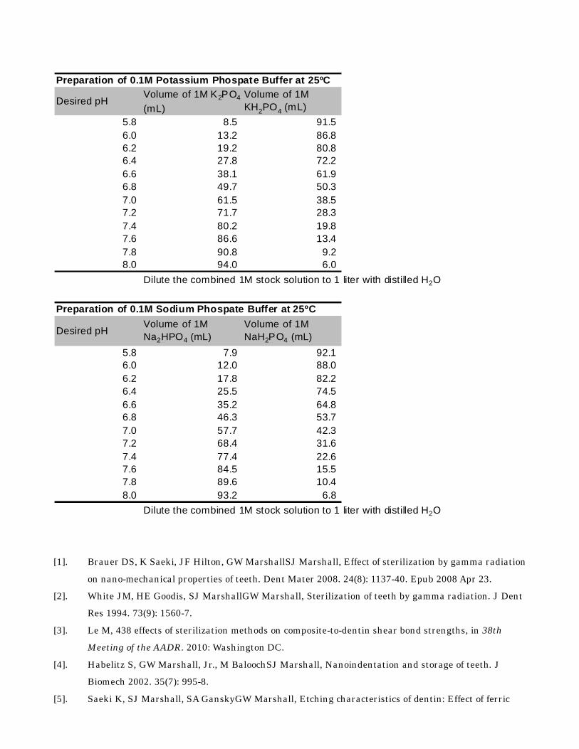
Preparation of 0.1M Potassium Phospate Buffer at 25ºC

Desired pHVolume of 1M K2PO4

(mL)Volume of 1MKH2PO4 (mL)

5.8 8.5 91.56.0 13.2 86.86.2 19.2 80.86.4 27.8 72.26.6 38.1 61.96.8 49.7 50.37.0 61.5 38.57.2 71.7 28.37.4 80.2 19.87.6 86.6 13.47.8 90.8 9.28.0 94.0 6.0

Dilute the combined 1M stock solution to 1 liter with distilled H2O

Preparation of 0.1M Sodium Phospate Buffer at 25ºC

Desired pHVolume of 1MNa2HPO4 (mL)

Volume of 1MNaH2PO4 (mL)

5.8 7.9 92.16.0 12.0 88.06.2 17.8 82.26.4 25.5 74.56.6 35.2 64.86.8 46.3 53.77.0 57.7 42.37.2 68.4 31.67.4 77.4 22.67.6 84.5 15.57.8 89.6 10.48.0 93.2 6.8

Dilute the combined 1M stock solution to 1 liter with distilled H2O

[1]. Brauer DS, K Saeki, JF Hilton, GW MarshallSJ Marshall, Effect of sterilization by gamma radiation

on nano-mechanical properties of teeth. Dent Mater 2008. 24(8): 1137-40. Epub 2008 Apr 23. [2]. White JM, HE Goodis, SJ MarshallGW Marshall, Sterilization of teeth by gamma radiation. J Dent

Res 1994. 73(9): 1560-7. [3]. Le M, 438 effects of sterilization methods on composite-to-dentin shear bond strengths, in 38th

Meeting of the AADR. 2010: Washington DC. [4]. Habelitz S, GW Marshall, Jr., M BaloochSJ Marshall, Nanoindentation and storage of teeth. J

Biomech 2002. 35(7): 995-8. [5]. Saeki K, SJ Marshall, SA GanskyGW Marshall, Etching characteristics of dentin: Effect of ferric

chloride in citric acid. J Oral Rehabil 2001. 28(4): 301-8. [6]. Helebrant, The influence of simulated body fluid composition on carnobated hydroxyapatite

formation. Ceramics 2002. 46(1): 9-14. [7]. Kokubo T, M Hanakawa, M Kawashita, M Minoda, T Beppu, T Miyamoto, et al., Apatite formation

on non-woven fabric of carboxymethylated chitin in sbf. Biomaterials 2004. 25(18): 4485-8. CDC has all guideline for disinfection.http://www.cdc.gov/hicpac/pdf/guidelines/Disinfection_Nov_2008.pdf

Protease inhibitors

metalloprotease inhibitors FW

benzamidine HCL

Benzenecarboximidamide,Benzamidinium chloride,Amidinobenzene hydrochloride 156.6 2.5 mmol/L 0.39 peptidase inhbitor C6H5C(:NH)NH2.HCl.aq

cysteine proteinase inhibitors

N-ethylmaleimide NEM 125.1 0.5 mmol/L 0.06

sulfhydryl alkylating agent thatinactivates NADP dependentisocitrate dehydrogenase andmany endonucleases. Reagentfor the covalent modification ofcysteine residues in proteins C6H7NO2

ε-amino-n-caproic acid 6-aminohexanoic acid 131.2 50.0 mmol/L 6.56

inhibit plasminogen binding toactivated platelets. Lysineanalog. Promotes rapiddissociation of plasmin, therbyinhibiting the activation ofplasminogena d subsequentfibrinolysis

serine protease inhibitor

phenylmethylsufonyl fluoride

phenylmethanesulfonyl fluoride,benzylsulfonyl fluoride, PMSF,alpha-Toluenesulfonyl fluoride

174.2 0.3 mmol/L 0.05

inhibit serine proteases such astrypsin and chymotrypsin. Alsoinhibits cysteine protease andmammalianacetylcholinesterase. Not aseffective or toxic as DEP.Effective concentration 0.1-1mM,Half-time=1hr at pH7.5. notsoluble or stable in Water. Stocksolution stable 1 month at 4C.

DEP

diethyl pyrocarbonate, ethoxyformicacid anhydride, diethl oxydiformate,DEPC

162.1 0.0 mmol/L 0

inactivates Rnase in solution atabout 0.1%,(v/v), thus protectingRNA against degradation.Modification reagent for His andTyr residues in proteins. O(COOC2H5)2

AFM Competency Check List

Your Name , Title Project: Trainer: Date: 1. Sample preparation

n Sample flat (E. G. F. P.) n Sample polished without scratches (E. G. F. P.)

2. Hardware --- Basic ---

n Know the switches and sequences to turn on and off system safely (E. G. F. P.) n Safely install and uninstall AFM head (E. G. F. P.) n Know how to use optical microscope (E. G. F. P.) n Safely insert and remove tip holder (E. G. F. P.) ² Handle tip holder without banging (E. G. F. P.) ² Enough distance between tip and sample (E. G. F. P.)

n Know how to change tips (E. G. F. P.) --- Advanced ---

n Know the difference of tip holders and modes (E. G. F. P.) n Understand the theory of AFM (E. G. F. P.)

2. Software n Know how to start and end program (E. G. F. P.) n Know how to set initial parameter for safe engaging. (E. G. F. P.) n Know how to change scan size, z-range and other parameters (E. G. F. P.) n Know how to capture image (E. G. F. P.) n Know how to manipulate captured image (E. G. F. P.) n Know how to move files from virtual drive (!:╲) to individual directory (E. G. F. P.) n Know how to export images (E. G. F. P.)

3. AFM Image mode n Locate the area of the interest in specimen (E. G. F. P.) n Smoothly lower tip to the specimen surface (E. G. F. P.) n Know how to adjust LASER for optimized signal (E. G. F. P.) n Engage and disengage safely (E. G. F. P.)

4. Misc. n Safely handle chemicals (E. G. F. P.) n Knowledge of infection control (E. G. F. P.) n Maintain lab clean and neat (E. G. F. P.)

Overall grade 1. OK to work independently, 2. Need to work under supervision, 3. Need further training session

Trainer’s Signature

AFM-Hysitron Competency Check List

Your Name , Title Project: Trainer: Date: 1. Sample preparation

n Sample flat (E. G. F. P.) n Sample polished without scratches (E. G. F. P.)

2. Hardware --- Basic ---

n Know the switches and sequences to turn on and off system safely (E. G. F. P.) n Safely install and uninstall transducer head (E. G. F. P.) ² Enough distance between tip and sample (E. G. F. P.) ² No banging and jumping of the head and tip (E. G. F. P.)

n Know how to change tips (E. G. F. P.) n Know how to clean tips (E. G. F. P.)

3.Triboscope software n Know how to set initial parameters (E. G. F. P.) n Know how to choose right area function (E. G. F. P.) n Know how to use torapozoid (E. G. F. P.) n Know how to calibrate system (E. G. F. P.) n Know how to export data in text format (E. G. F. P.)

4. Nanoscope software n Know how to start and end program (E. G. F. P.) n Know how to set initial parameter for safe engaging. (E. G. F. P.) n Know how to change scan size, z-range and other parameters (E. G. F. P.) n Know how to capture image (E. G. F. P.) n Know how to manipulate captured image (E. G. F. P.) n Know how to move files to individual directory (E. G. F. P.) n Know how to export images (E. G. F. P.)

5. Nano-indentation mode n Locate the area of the interest in specimen (E. G. F. P.) n Smoothly lower tip to the specimen surface (E. G. F. P.) n Engage and disengage safely (E. G. F. P.) n Safely make indentation using 2 computers (E. G. F. P.)

6. Misc. n Safely handle chemicals (E. G. F. P.) n Knowledge on infection control (E. G. F. P.) n Maintain lab clean and neat (E. G. F. P.)

Overall grade 1. OK to work independently, 2. Need to work under supervision, 3. Need further training session

Trainer’s Signature

AFM-Hysitron configuration

This system is multi mode.Image with contact or tapping mode or STM mode for

nano-indentation / DSM with Hysitron.All cables, extenders and scanners must be connected

and configured correctly.

AFM base with Non-extended connector

nPoint scanner with 2D Hysitron head

Default setting

nPoint controllerBuff color cableà front of AFM controllerGray flat cable à AFM base

AFM controller Buff cable– connect to back of nPoint

Back of nPoint

To use contact or tapping mode for imaging, need Quadrex box – for both

Veeco and nPoint scanner

Quadrex Extender Extended cable

• Extended cable can be found in the drawer

Default Setting – nPoint scanner for Hysitron indentation

nPoint controller

AFM base

Use non-extendedconnector

AFM controller

AFM SoftwareClick “di” menu at upper left cornerSelect “microscope select”

Use nPoint without QuadrexBNC connects to Blue Box

Serial cable goes to back of AFM PC

nPoint scanner

nPoint scanner for imaging with Quadrex

nPoint controller

AFM base

Use extendedconnector

AFM controller

AFM Software,Click “di” menu at upper left cornerSelect “microscope select”

Use nPoint Quadrexed

AFM optical head should be the one with vertical and horizontal adjustments

BNC connects to Blue Box

Serial cable goes to back of AFM PC, COM3

nPoint scannerQuadrex

Serial cable goes to back of AFM PC

Veeco scanner for imaging and indentation with Quadrex

nPoint controller

AFM base

Use extendedconnector

AFM controller

For AFM SoftwareClick “di” menu at upper left cornerSelect “microscope select”

Use Veeco with Quadrex

Both AFM optical heads can be used.

BNC connects to Blue Box

Serial cable goes to back of AFM PC, COM3

VeecoJV scannerQuadrex

Cable connections for AFM-Hysitron system

Desktop PC nanoDMA Module TRIBOSCOPE DSP Lockin Amp Nanoscope ADC5 AFM base

SIG SIGNAL INPUT, A / IPHA CH2 OTUPUT Aux 4AMP CH1 OTUPUT Aux 3AC SIGN OUTN15 -15VP15 +15V

PIEZO

TRIBOSCOPEMICROSCOPE FEEDBACK

Hysitron board COMPUTER

CONTROLLER DATA ACQUISITION

USB GPIB

* N15 and +15V are connected skinnier cable (with "DACOUT" tag on* others are connected by cable class; 60 C, 30V, 20AWG

COM1 (Serial) nPoint controllerCOM3 (Serial) Quadrex extender

Reference Layer techniques for AFM Marshall group has 4 techniques developed in past 10 years.

1) cyanoacrylate 2) masking with tape 3) glass 4) nail vanish 1) cyanoacrylate method.

• Pros. Easy to prepare. Durable for clinical strength acid etch (10% citric, 35% phosphate). OK to use NaOCl if it is weak?

• Cons. Penetrate dentin tubules and change mechanical properties near the cyanoacrylate layer. Separates if dehydrated (SEM, dehydration study)

• Application Repeated treatment with less corrosive chemicals

2) Masking tape method 3M photo mounting square has been exclusively used

• Pros. Easy to prepare. Durable for clinical strength acid etch (10% citric, 35% phosphate) for shorter treatment time. There is no separation for rehydrate-dehydrate study or SEM analysis in vacuum.

• Cons. For longer treatment time, adhesive seemed to leak, does not provide good protection to obtain control layer. For acetone based primers, adhesive seemed to dissolve and contaminate the surface. Tape did not stay stuck when treated with NaF solutions.

• Application Short treatment with less corrosive chemicals. It is recommended to check if the adhesive of the tape does not dissolve for the chemicals to be used. It is also recommended to monitor if there is no residue of adhesive left on the specimen surface with AFM, when you use a new batch. (manufacturers tend to change the product without disclosing it).

3) Glass reference A small piece of micro slide glass is bonded to the specimen

• Pros Glass reference is the most durable against repeated and longer acid treatment to measure the height change with AFM.

• Cons Glass reference is hard to bond together and polish. It can separate if it is desiccated.

• Application

Long time kinetics study, repeated height measurement with AFM

4) Nail Vanish Thin layer of nail vanish is painted to mask the area to be protected from the treatment. After the removal of nail vanish either by carefully wiping it off with acetone, the protected area will serve as a reference layer. A special color, Revlon Cherry in the Snow is recommended by Dr. Featherstone’s lab after their extensive study. • Pros

Good for the long term treatment which does not require repeated measurement of the specimen. Can protect the entire specimen (pulpal side, side wall etc.) so that treatment effected surface can be limited.

• Cons Nail vanish can penetrate the margin area. Be cautious when you measure mechanical property around the edge of the treated area. Removal of vanish either by polishing or wiping with acetone can be tricky. Cannot use with acetone or alcohol containing solutions.

• Applications Long term acid etching / demineralizing treatment. Treatment requires submerging specimen in the liquid. You should check if the treatment solution will dissolve the nail vanish before starting the experiments. In 2010, Anora compared effect of nail vanish method used by Megan to tape method used by Luiz. She also established a standard method so that the ratio of exposed dentin and the quantity of acid is consistent for all remineralization-demineralization studies. àRefer to the manual written by Anora.

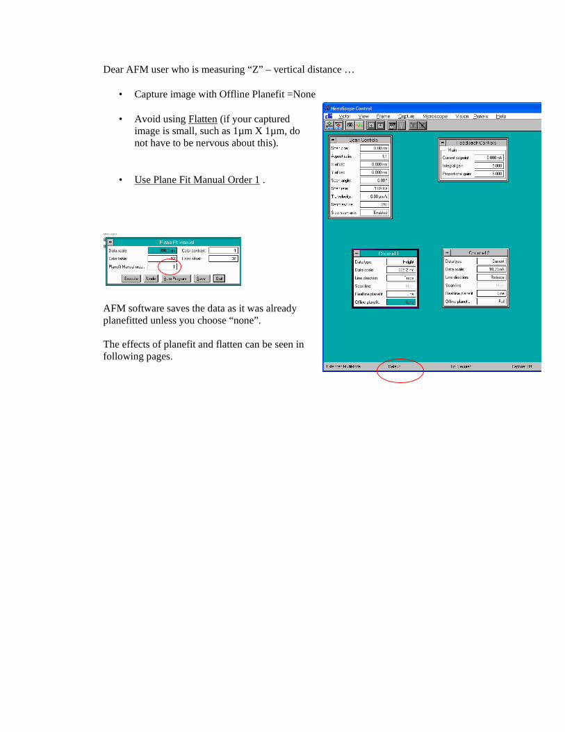
Dear AFM user who is measuring “Z” – vertical distance …

• Capture image with Offline Planefit =None

• Avoid using Flatten (if your captured image is small, such as 1µm X 1µm, do not have to be nervous about this).

• Use Plane Fit Manual Order 1 .

AFM software saves the data as it was already planefitted unless you choose “none”. The effects of planefit and flatten can be seen in following pages.

1. Acquiring data1. Reference layer ( more than 30% of image)2. Off-line planefit must be “None”

• Captured image will be modified by software• Full : A best fit plane which is derived from the

data file is subtracted from the captured image.

2. Modification of data.1. Some modification command distorts file’s

height information

• Original• The image has slight

bow along the Y-axis

Order2 : Bow is removedThe scan lines are aligned

Order 1 : removes Z offset, tilt

Order 3 : removes Z offset, tilt and bow

•Order 2 : removes Z offset, tilt and bow

Z=181

Order 2 :Correct bow (V+H)Correct tilt (V+H)

Order 3 :Correct bow (V+H)Correct tilt (V+H)

Order 1 : Correct tilt (V+H)

Order 1 : Reduce noise.Correct tilt (V+H)Correct bow (V+H+Diagonal)

Order 2 : Reduce noise.Correct tilt (V+H+Diagonal)Correct bow (V+H+Diagonal)

Order 3 : Reduce noise.Correct tilt (V+H+Diagonal)Correct bow (V+H+Diagonal)

Z=170.6

Z=179.2

Z=179.4

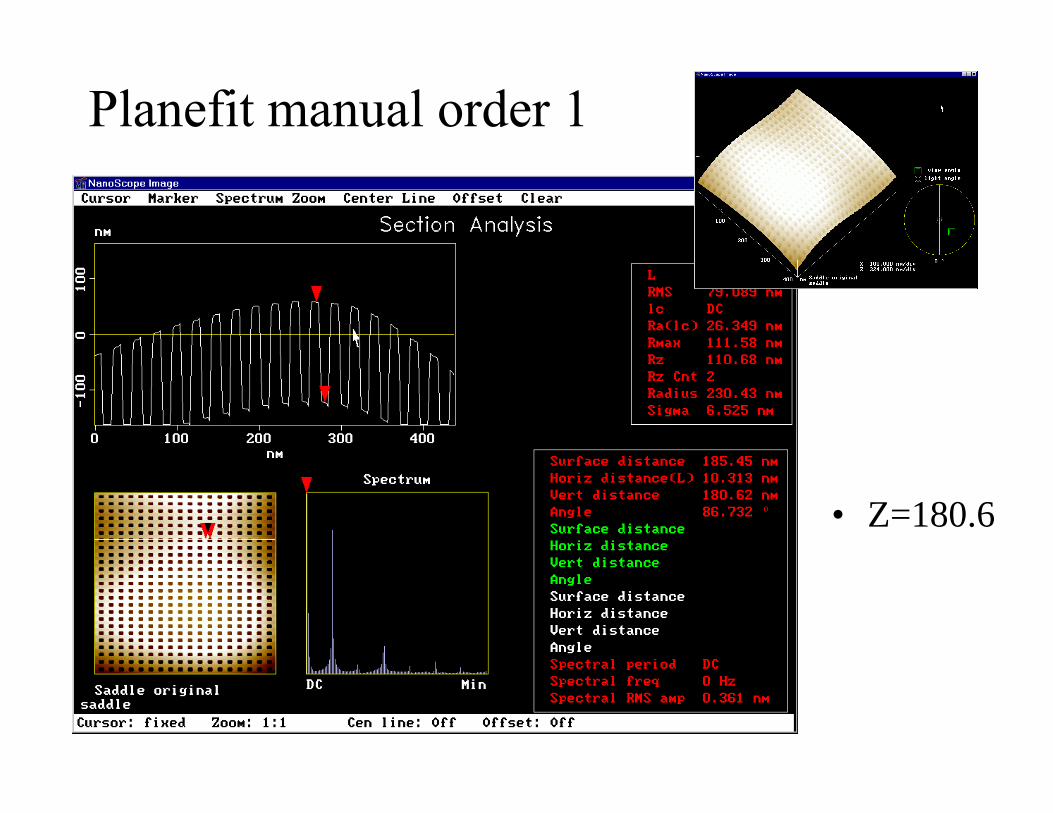
• Z=180.6

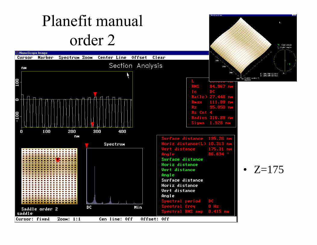
• Z=175

• Z=173

Acid etching – kinetic study with AFM Sample size

• N=6 (4 disks for each concentration of acid) • 6 measurement of intertubular dentin for each treatment time

Acid Lactic acid Buffer, Ca, P (2.2mM) , pH 5 . (From Featherstone’s lab) –aim 1, page50 Treatment time: cumulative time up to 30 min.

0, 5, 10, 15, 20, 30, 60, 120sec 300(5min), 600(10min), and 1800

(30min)

**Dental material 2001, GW Marshall et al. (Citric Acid, pH2.5, 0.018M) AFM imaging

• 50 x 50 micron • Wet cell (DI water) • 6 measurement of vertical distance between selected area and

reference layer

AFM study - same area measurement technique Materials, instrument

• Beaker – 100cc • Disposable dish • Cotton pliers • Sponge pellets for acid

etching • Acid • Dropper

• DI water • Timer • Transparent sheets • Sharpie • Scotch tape

1) Sample preparation

i. Dentin – dentin disk, occlusal section (perpendicular to dentin tubules), reference layer embedded, embedded in Coe-Tray, polished to 0.25micron.

ii. Selection of reference layer – see reference layer guide –

2) Selection of the area image – collecting information

• Reference layer and dentin were tightly bonded • Only 2 or 3 rows of cyanoacrylate plugged dentin tubules from reference layer

*Scout the quality of reference layer with light microscope. Add a line or two with razor blade with light pressure near the area you have chosen. These lines will serve as a guide to go back to the exactly same area through the study. Tips for good recovery to the same spot

• Include reference area and/or scratch in the image • Mark land marks on monitor screen (Use transparent sheet)

• Make a guide sheet of the first captured image (Use transparent sheet) • Mark sample and stage before moving the sample out.

3) Etching kinetics experiment

a. Capture baseline (0 sec) image Capture image by clicking camera icon. Captured files are stored in “!” directory Remove specimen from the AFM stage.

• Change AFM’s offline capture setting to “no fit”. – very important • Select the area with tight contact between reference and dentin. • Reference layer should occupy at least 30% width of the image. • Tape a transparent sheet on CRT monitor and AFM image monitor • Record information on the CRT transparent sheet such as position of reference layer,

scratch and tip shape. • Record information on AFM image, reference layer, dentin tubules. • Capture 2 locations per specimen

b. Acid etch • Apply the acid to the surface with the sponge or use the dropper. • For shorter etching time, quench the specimen disk in DI water in the beaker to stop the

reaction. • Keep the specimen moist or wet in DI until measured • Look for the exact same location using the transparency map created in step 3) • Capture images

crack

scratch

Z Measurement Refer to the PowerPoint Manual “Measuring Z” Nanoscope software off-line operation Important !! All the captured image files are named with the time and extension “001”. We call this file RAW data. Do not overwrite, modify otherwise loose RAW image. When you are moving to another image or you made changes, you will be prompted if you want to save change. Click yes if you want to save the change. Remember to change extension to something like 002, 003. Move and Save file File management

Since limited number of images can be stored in “!” drive, please move your image to your own directory/ drive when you finish your work for the day. You have to use the “Browse” command before you transfer the data files to CD. Your files can be viewed, modified, analyzed with the desktop version Nanoscope software. (Windows version only).

After captured files are moved to E drive, they can be handled with the regular Windows operating system to be copied to CD.

Highlight the file you wish to move by clicking it. Select “File” à “Move” Type in the destination folder, such as “E:\your folder. To move multiple files use wildcard ‘*’ Example)

If you want to move all files captured on August 19, to directory “bill” in E drive, Type From …. “0819*.* To ……..e:\bill

Modifying and analyzing the image file 2-D and 3-D view Click the icon on toolbar. Click NOTE to enter any information How to print out image

• We do not have printers connected to the AFMs. Options to print out the images include • Export in TIFF format file – viewable from any imaging softwares – then copy to CD . • Paste images to PowerPoint file. • Take AFM files via CD and use offline Nanoscope software then do the same 1) Export in TIFF format

i. View the image with 2D or 3D views ii. Click Utility and select TIFF export iii. Save with TIF extension to the folder.

2) Using PowerPoint or word with TIFF i. Export in TIFF format ii. Open PowerPoint. iii. Insert→picture→From File iv. Select your image file v. You are able to change the size of image after you import the image

3) Using PowerPoint or word with screenshot i. Use “ALT”key and “Print” key (hit together) to capture the screen. Only active window will be

captured. ii. Open PowerPoint, Use “paste” command.

Some useful windows shortcut commands Ctrl + C à Copy Ctrl + V à Paste Win + E àOpen Explorer Alt + Print à Capture screen Alt + F4 à Close active window AFM computer system

A: 3.5inch Floppy Disk drive C: Hard disk drive for operating system ! : Virtual drive in D: for storing captured data E: Hard Drive. We store the data in this disk F: CD-DVD writer

Dear AFM user who is measuring “Z” – vertical distance …

• Capture image with Offline Planefit =None

• Avoid using Flatten (if your captured image is small, such as 1µm X 1µm, do not have to be nervous about this).

• Use Plane Fit Manual Order 1 .

AFM software saves the data as it was already planefitted unless you choose “none”. The effects of planefit and flatten can be seen in following pages.

Measuring “Z” change-etching kinetics study-

Kuniko SaekiSummer 2008

Contents• Word document

– Study design– AFM imaging – data acquiring– Etching experiment– Basic of captured data processing

• How to save, move, copy and print, using different devices• Z-measurement for kinetics study

– AFM image requirement– Plane fit on the reference layer

• Using “section” command– Select the areas to be traced

• Print a guide map – how to use PowerpointTM functions– Measuring the height difference on each image– Summarize measurements using excelTM spread sheet

• Appendix - “excel sheet for entering data”

Requirement for captured image

• Offline Plane fit must be “OFF” when the image was captured.

• Reference layer occupies around 30% of the image

• You can identify the area that dentin tubules were not penetrated by the cyanoacrylate

• No garbage on the surface

Test the first captured image for reference layer adequateness

• Usually sample is tilted slightly and has to be corrected.

• Click “Modify” à “Plane Fit Manual”.• Select “Order” =1

• Draw a Y line, erase the part except on the reference layer, then execute.

• Draw X line on the reference layer, erase the part on the voids etc, then execute.

• Change “Data scale” as needed

• Do not use “Flatten” command – you will loose “z” distance information.

• Go to Section command by clicking knife icon

Make sure if reference layer is plane fitted flat

• In the section command screen…• Draw a line on reference layer,

both X and Y direction. • If it is not flat, go back to planefit

command and adjust until you get flat reference layer. This is very important procedure to make good measurement.

• Save the file with different extension, such as “07142015. 002”

Making a map -1• It is usually good to use the

image of the first etched image as a map.– Hidden dentin tubules tend to

be revealed by being etched• Click Top View command

icon.– Adjust image as needed by

changing “Data scale, color contrast, color offset, etc..

– Use “Note” to add description to your image.

• To export image, Click “Utility” -> “TIFF Export” command.

• Type in Destination and file name with “tif” extension.

Example of images

Baseline (left) has less tubules revealed than etched (right)Bottom (cyanoacrylate reference layer), AFM, wet

Import TIF file to PowerPoint

• Open PowerPoint• Select layout by clicking

“Format” à” Slide Layout” –“Title and Content” works easiest

• Importing TIF image– Click picture icon in the center

of the slide.

– Locate to the folder you have saved Baseline TIF file. Then click “Import”.

Making a map -2

You can do same operation by clicking“Insert” à “Picture” à”From File”

Making a map -3PowerPoint skills

1. Add title to the slide so that you can recognize the image later.

2. Trim off un-needed portion of the image with “picture” toolbar

3. Click on the image, picture toolbar should appear. Click “Crop” icon. Your mouse pointer should change into “crop” shape.

4. Trim the image as you need by dragging borders of the image

• If you click the outside of the image object, “crop” function is cancelled. To activate it, click the image then “Crop” icon on the toolbar again.

Picture object – move, change size, rotate – borders marked

with white circle

Picture object – cropbordres marked with bold

black line

Making a map -4PowerPoint skills

1. After trimming, make the image size bigger.

2. Save the file.

3. You can print out and manually write in where you are going track or use PowerPoint to draw them in before you print this out.

To print, click “File” à “Print” and select “Current slide”.

Note : Both our AFM PC are not connected to printers. You have to transfer PowerPoint file to the PC with printer.

To change the length of the line,click on the line when you see white circle at the ends, left click on the circle (do not release the button) , drag to extend or shrink the length or rotate, then release the button

To move, left click on the line, drag the line while holding the mouse button. Release button at the destination

To change the color, size and shape of the end, right click the line and select “Format AutoShape” from the window

Change the Style and Color of the Line, Style and size of Begin and End so that they are clear on the AFM image

PowerPoint skills - How to draw lines

1. Click “Arrow” icon on the Drawing toolbar

2. Draw a line by dragging the mouse• Left click at the starting point, do not release the button• Draw a line until the end point by dragging, then release the button

To move, left click on the text, you should see the outline of textbox. Move your mouse pointer to the end of the textbox. The shape of the mouse pointer changes to the “Cross shape”. Then you can click the border and, drag the textbox while holding the mouse button. Release button at the destination.

To change the color, font and size of the text, right click the textbox and select “Font” to open “Font” window.

To change the style of the textbox (fill and line) right click on the text box and select “Format Text Box”.

PowerPoint skills - How to add textbox

1. Click “Textbox” icon on the Drawing toolbar

2. Click on the slide and start typing your text Text Box

Text Box

Example of the map• Choose spots to be tracked

– 6 spots for intertubular dentin (and 6 for peritubular dentin).

– Avoid area too close to the reference (cyanoacrylate may be infiltrated)

– avoid the edge of the image • Lines are easily moved. Please

make a print out. (Hardcopy)

• If you do not see those toolbars, click “View” à “Toolbars” and make sure they are checked.• Picture toolbar only appears when you click on the objects in picture format.

Picture Toolbar

Drawing Toolbar

Measuring the height difference with AFM software

• After you decided which 6 locations to be tracked and printed out the map, go back to the AFM software.

• Plain fit all the captured files.• Open the file to be analyzed

• Click “section analysis”

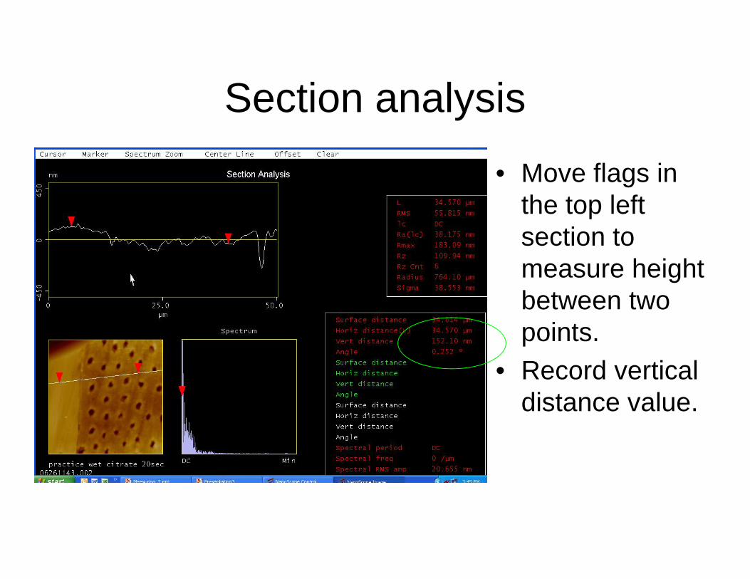
Section analysis

• Move flags in the top left section to measure height between two points.

• Record vertical distance value.

Summarize with Excel• Record all the vertical

distance measurement

• Average 6 measurements from each site to get 2 measurement for each treatment time

• Subtract the baseline value to obtain the etched value

Nanoindentation Hints

Version 1.0

December 25 2005

Kuniko Saeki

Marshall Lab PRDS UCSF

1

Nanoindentation hints 1. First things to do prior to experiments.

a. Turn on the black Hysitron box (need to warm-up, 2 hours recommended)

b. Final polish the specimen (0.25 to 0.01 µm) keep it dry or moist c. Turn on AFM

1. Turn on the box under the desk. Switch is at the right back side

2. Turn on the AFM PC, if it is not on. Open NanoScope version 5.12r3

2. Prepare Hysitron computer • You may want to reboot the PC, while doing this, turn off the Hysitron box. • Open “Tribo scope” software • Find a transducer in a black plastic box. Turn the power off while connecting it to the

Hysitron box (backside), turn the power back on. • Check if the initial setting values match to those on a info sheet in the black transducer box

by Clicking “setup indent” à “Set Transducer Constants” icon

• • • • • • • • • • •

Switch is here! Usual setting for 4 dials are: a. Low Pass filter: 300 b. Output Gain 1 : 1000 c. Output Gain 2 : 1000 d. Display : 100

*Check Displacement Scale Factor matches to the value on the sheet *Max Force is smaller than the value on the sheet *Machine compliance is 1.7 for black shaft tip, lower for white ceramic base(0.8) Please refer to the note on the wall for right machine compliance value for individual tip.

2

• Drift correction Click “setup” à drift correction. Drift correction: change to 2 sec.

• Spring force compensation should be checked “V” too.

3. Prepare AFM

• Remove the optical lens. • Flip the switch to select STM • Click “microscope icon”, select “STM” mode. • Type in initial values for engaging (do not engage, yet) à refer Appendix D • Set up fused silica quartz reference on the stage. • Lower the stage to have enough clearance before placing the indenter by using lever (to

UP) • Place the transducer+indenter over the silica reference.

4. Air indent to adjust Electro static force constant. Open load function “air indent new” (Loading 10sec, Unloading 10sec, peak force 600uN)

From indent screen, click setup à Advanced Z-Axis Calibration, following window will pop-up. Click “Calibrate Transducer”. Instruction window will appear. Click Yes if you are ready.

3

1) Change Displacement Gain to 100 (usually it is 1000 for the real measurement) and change Output 1 Gain and Output 2 Gain dials on the front panel of the hysitron box to 100 (1000 for measurement also).

2) Make sure “Displacement Scale Factor matches the value on the sheet in the transducer box. 3) Click Done

Click Yes if you already chose “air indent new.ldf” . If you click “No”, the program will stop at this point. You have to close all the open windows manually, then select right load function and start z-axis calibration again. ( I think this is one of the bugs in the newer version software they’ve installed after upgrading PC. I inquired about possible bug fix, but haven’t heard from hysitron, yet. I can remove this sentence since right load fuction should be already selected if the user followed this instruction. --Kuniko)

Use two dials in front of the hysitron box and adjust display value to 0.00., click OK. You will see real time plot window display force displacement curve going downward on the screen.

Output 1 Gain and Output 2 Gain dials

4

Readjust the dials to 0.00. and click OK. You will see Curve Fit Plot ESF vs. Displacement screen. If the blue line is fitted straight up. You have successfully finished calibration. (Sally, I will add bad example if I luckily get one in next revision)

New values were automatically imported to the setting. Close “Advanced Z-Axis calibration” window. Before starting experiment go back to setupà Calibration. Change Displacement Gain back to 1000. Change Output 1Gain and Output 2 Gain to 1000 on the Hysitron Box.

5. Indentation to fused silica standard

5

a. Click “open load function” icon from “set up indent” screen, choose “trapozoid3j.ldf” to be ready to make real indents.

b. Type in the value for the “Peak Force” (usually we start with 8000 µN).

6. Select an Area Function File (calibration file)

• From Set up indent screen, click “Define Area Function” icon • Click “Open Area function” icon

• Select an area function file (Check tip number and wet/dry condition, right for your

application) and load it.

7. Indentation to Reference • Lower the indenter very very close to the surface of the fused silica by using lever on AFM,

use binoculars for magnified view. • Adjust Hysitron box to approximately “00.00” • Make sure Scan Size is “0” at AFM computer • Make sure gains are connected, i.e. different from 0 • Click Green Arrow icon to engage

If you can not engage (false engagement, z position bar drops to limit), you have 2 options to try. Option 1: Disengage. Then increase value of setpoint, integral gain and proportional gain. (8, 8 and 8, 10, 10 and 10, instead of 5, 5 and 5). If you still can not engage with higher values, you should consider the contamination of the tip or specimen surface or the tip is broken. Option 2: Click “Motor” and “Step motor” and manually lower the tip until it engages correctly. (z : -20 to 20 V). To safely do this, please do following. Type “0” in setpoint box, then adjust display of hystitron box to “00.00” manually with “zero” dial. Then type the value you used to engage (such as 5) back into the setpoint box to control the force of contact, Use stepmotor function to move the tip up and down. After the z-range bar is in good position, repeat typing in “0” in setpoint box and confirm the hysitron box displays “0”, before you move on.

Change Peak Force to 8000

6

• Increase scan size (10 to 30 µm) • Look for a flat clean area to make indentations. • Offset to the area (Click offset à execute), then change the scan size to “0”. • Is the Hysitron computer side ready to indent? (setup indent screen is on with correct value

typed in, no large drift observed in hysitron box display) • Change integral gain and proportional gain to “0”. • Immediately click “Make Indent” in the Hysitron side.

8. After the indentation is completed, save file screen will pop-up. Then you must immediately

change the integral and proportional gain back to 5.0 (or something you are using) with the AFM computer.

9. Save the indentation file. Use filename easy to identify it. Factors suggested to be included in the filename; (load, wet/dry, material), For example, if you nanoindented a dentin sample 1, with 400uN load in wet cell, you can name the file as “den1-400w-1”.

This kind of screen will appear after you save the file. Change “Unloading segment” to “3” and “Lower Fit %” to “65”. Then Click “Execute Fit” to have Er and Hardness value calculated.

You have successfully completed one indentation now! Accepted Er and Hardness values on standard (Silica glass) are Er: 69.6 (65-75) GPa, H: 9.5 (8.5-10) GPa Important!! Please record the values in Log Book.

10. Repeat indentations on standard with smaller peak forces such as 4000, 3000, 2000 to confirm the system is calibrated and working properly.

• You do not have to disengage the tip if it is working happily at the right z-limit (-20 to 20) • Use X or Y offset window in AFM PC to manually move the tip to a new position.

7

Berkovich tip has a triangular pyramid shape, if you indent with a large load or have a soft sample, you will have a large indented and deformed area. In these cases, make sure to move the tip far enough from the adjacent indents. On silica standard, separate indents at least 5µm with more than 5000 µN load.

11. Scan the area you’ve indented to evaluate the shape of indents after finishing the series. • Increase Scan Size in AFM PC by 10 to 20 µm. • Indents should be equilateral triangle shape for Berkovich indenters

Example of good indents

12. Disengage the tip by clicking red arrow in AFM PC 13. At the end of the experiment please do following procedure to make sure everything is working in

good condition for your colleagues. • Clean the tip (Follow the instruction ) • Make an indent with 8000 µN peak force to the fused silica • Save the file on “Daily Log” folder on desktop • Record the values in blue log book.

14. Indentation of your real sample.

• Follow the same protocol. • Record “Set Point” value, “Area Function” you used in your lab notebook. • Indent depth around 150nm is ideal.

Example of elongated indents

8

Sample preparation hints • Height should be less than 2.5 mm, more than 0.5 mm • Surfaces are polished parallel. • Sample has to be glued to the metal stub using Cyanoacrylate adhesive (RDS Inc). You cannot

use double stick tape. (You end up with measuring modulus of the tape) • Be aware if the glue infiltrates or crawls up the sides of your sample and alters mechanical

properties. (use minimum amount of glue. Sample has to have enough thickness after final polish after gluing)

Indentation using wet-cell

• Prepare a plastic ring from a clear test tube • Make a thin rope of blue periphery wax • Assemble sample and ring with periphery wax, so the wax seals the entire ring. • Add liquid in the wet cell using dropper or syringe. Depth should be half of the length of

indenter but should not touch the transducer. • Transducer and Piezo scanner are not waterproof. They can die if you wet them accidentally.

This experience was costly. • Perform indentation on fused silica reference in wet cell. • Use Area function for wet measurement.

Transferring the data to text or excel format

1. Select right “Area Function file” for the data executed and exported. 2. Click “Multiple curve analysis” icon. Add files to be exported, click OK.

3. Then, name the file and save. Hysitron software will automatically execute fit the area function and save it in text format, which you can open from Microsoft Excel.

9

Cleaning the tip. Please get training if you are not familiar with indenter cleaning.

--- How to clean indenter --- 1. Turn off hysitron box 2. Dip Kim-Wipe strip or Q-tip in acetone or ethanol, gently wipe the tip of the indenter. Acetone can

be found in yellow flammable cabinet in big lab(Rm.2201) 3. Rinse with DI water, gently dry with canned air 4. Screw back to the transducer and turn on the hysitron box

Calibrating a tip (Making new area function file)

See Appendix C

Trouble shooting 1. Indent shape is not equilateral triangle.

a. Indenter was bent!! b. AFM scan rate and angle is making false elongation of image. à change scan angle

and rate c. Indent was not done correctly e.g. false engagement, set point etc. d. Sample surface is not perpendicular to the tip e. Tip is contaminated.

2. Value of Hysitron box keeps drifting in wet-cell measurement. a. Possible leakage of liquid!! b. Air bubbles are trapped on the indenter or sample surface c. System has drifted, test for drift at scan size = 0, put current set point = 0, Hysitron

display should show 0.0; if different, zero the system and put current set point back to its initial value (probably 3 and higher)

3. Cannot get good image

a. Tip may be contaminated. àDisengage and clean the tip b. Integral gain and Proportional gain values are incorrect. c. Scan rate is not correct

4. Transducer making funny buzz noise.

a. Board and transducer tend to oscillate if you have been working for long period. à Disengage the tip. Turn off the Hysitron box then shutdown the computer. Let the AFM have a nice break.

10

Appendix A. Materials currently used

• Cyanoacrylate adhesive (RDS Inc) • Periphery Wax (Surgident, Heraeus Kulzer Inc.)

Appendix B. Currently used system

• Multimode AFM Nano Scope III (DI instrument) o Nanoscope software 5.12r3 o Piezo Scanner : 4875jv

• Tribo Scope (Hysitron) o Tribo scope software v4.0.0.0 o Sensor bias setting : -0.0320(V) o Machine compliance: Unique for each tip.

1.7 for black shaft Berkovich tip, 0.8 for white Berkovich ceramic shaft tip. o Berkovich indenter, 142.3°, 100nm tip radius

• On the transducer information sheet o Transducer ID: S/N5-060-68 o Z axis o Tare: -348mg o Load Scale Factor (Force): 1mV/mg o Displacement Scale Factor (Deflection): 20.015mV/µm o Electrostatic Force Constant: 0.0278 µN/V2 o Self Calibration Check: 476 mg o Maximum Force: 10.008mN

How to do new area function Step 1: Run several indentations on silica, 2 each, for example, 8000, 4000, 2000, 1000uN, add more if you wish.

Step 2: Click plot multiple curve, add curves, confirm all force-displacement curves aligns well. Step 3: Click multiple curve analysis. Choose the indentations you have made on silica Step 4: Save .txt file where you can locate easily Step 5: Click calculate area function

Step 6: Select the file you made in Step 4

Step 7: click “Load”. Following window will appear, do not change anything (this is standard Er for silica), click “OK”

Step8: Click execute area fit. If you see some dots do not align well, discard those indentation from Step 2 and re-do the steps.

Type in C0 value berkovich indenters = 24.5 cubecorner indenters =2.598 Clear values in C1 – C5 boxes by typing “0” in the boxes.

Step 9: If you like your new curve, click “save area function” icon.

How to run four point bending test with ELF3200

August 2007 Kuniko Saeki

Turn on PC- there is no password. -This will turn on ELF3200, too. - 1. Open WinTest program by double clicking desktop icon Ø Open Test project MS 6-1-07.prj (saved in EnduraTEC folder) Ø Open Test file File – For example, “Kuniko straight ramp-2.gf1”

2. Check Limits – Most Important!! –

Machine’s capacity is around -50(N), make sure Load is set in reasonable range (-20) and action is “Shutdown”

Define the Limits

Test file name should appear here

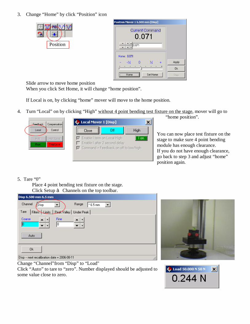
3. Change “Home” by click “Position” icon

Slide arrow to move home position When you click Set Home, it will change “home position”.

If Local is on, by clicking “home” mover will move to the home position.

4. Turn “Local” on by clicking “High” without 4 point bending test fixture on the stage, mover will go to

“home position”. You can now place test fixture on the stage to make sure 4 point bending module has enough clearance. If you do not have enough clearance, go back to step 3 and adjust “home” position again.

5. Tare “0”

Place 4 point bending test fixture on the stage. Click Setup à Channels on the top toolbar.

Change “Channel”from “Disp” to “Load" Click “Auto” to tare to “zero”. Number displayed should be adjusted to some value close to zero.

Position

6. Waveform Click Wave form icon to open the window Use “Ramp” setting. 0.016660mm/sec equals to speed=1mm/min 7. Click “Data Acquisition” à “timed data” on tool bar. Click “Browse” to set filename to be used for exporting data. Check mark “Export on Closing” and others as shown.

Type in a new name to be saved then click “Open”

8. Now we are ready to break beams. Ø Before loading sample in the test fixture, click local à click “high”. Loader will jump with loud noise.

Ø Load sample in the test fixture, place the fixture under the mover and click runà”ZeroStart”. Click Zero Start

Ø Open data acquisition window

Ø Click start for data collection, when mover is closer to the sample and/or you see negative number in

“load” window. Ø When it is done, click red button to stop. You may ignore shutdown warning. Turn Local “off” if Local

button remained green.

Export data will automatically start, do not disturb it. Exported txt data can be viewed with Excel. Important When closing software UNCHECK update to avoid overwriting current Test Project file settings

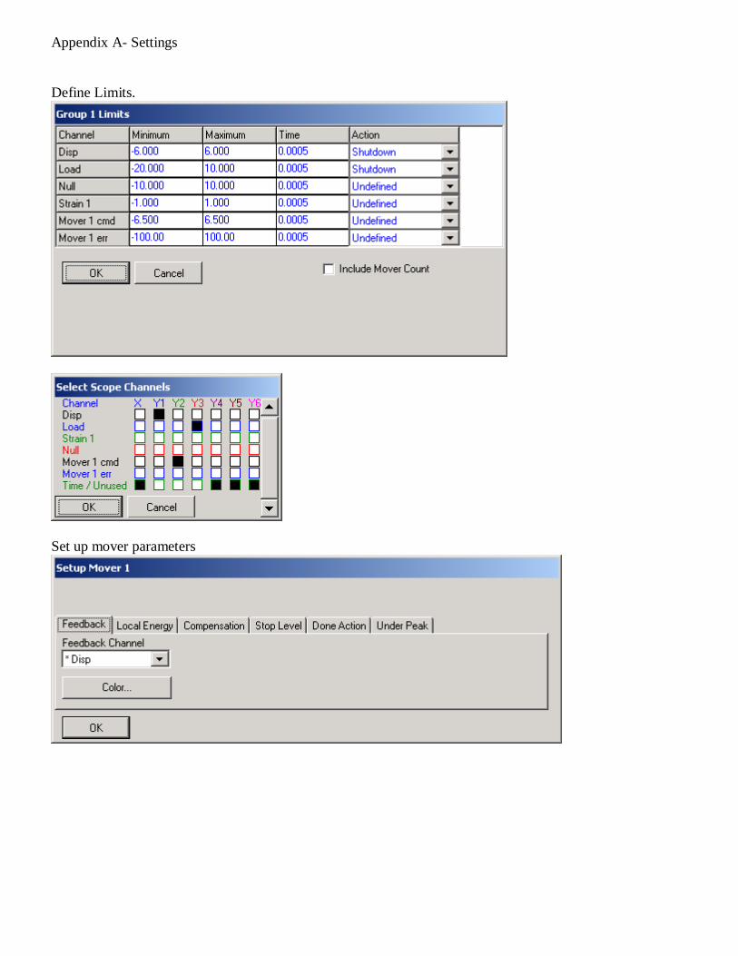
Appendix A- Settings Define Limits.

Set up mover parameters

How to get Load-Disp curve from ELF3200 text data- using macros My experience of modifying text data files exported from ELF3200 to usable Excel format is time consuming with repeated maneuvering. I am showing three ways to achieve this task. 1) You can use macros I wrote 2) Write your own so that you do not have to lower security level to accept mine 3) Do everything manually. 1) Use macros provided “4point macro book.xls” available from web upload To use this macro file, your security setting of excel has to be changed to medium. n Open excel n click “tool” on toolbar à Options n click “Security” tab then Macro Security n Select “Medium” n Restart “Excel”.

Try to open “4point macro book.xls”. Click “Enable Macros” if you want to use this macro file. Keep the file open while working on ELF3200 text files.

File – Open, select data txt formatted file.

Click Dlimited Then click comma, then finish.

You have a text file opened in correct format now. Please note that ELF3200 enclosed two rows of headers in every 20 points it measured (left). Number of scan points you used when you run ELF3200 reflects the 20 rows in one set here. (shown below). 20th point of each set is recorded repeatedly as measurement point 1 in the following set, thus you have to clean up one.

1. First Macro (Macro_4point1) will do following tasks. n remove extra headers. n Add one line between header and numbers n Select all data ( Ctrl+shift option is quick to select all), then sort data by Column A

Click “tool” à “macro”, select the macro, then click “Run”. If you do not see a list of macros, make sure Macros in: All Open Workbooks is selected.

2. You have to manually remove rows contains headers and “20”.

n Find first row, where Column A is “20”, select cells

in that row, type ↓arrow while holding “Shift” and “Ctrl” keys together, this will select all unneeded rows so that you can delete them at once.

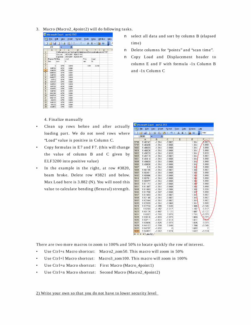
3. Macro (Macro2_4point2) will do following tasks. n select all data and sort by column B (elapsed

time) n Delete columns for “points” and “scan time”. n Copy Load and Displacement header to

column E and F with formula -1x Column B and -1x Column C

4. Finalize manually

• Clean up rows before and after actually loading part. We do not need rows where “Load” value is positive in Column C.

• Copy formulas in E7 and F7. (this will change the value of column B and C given by ELF3200 into positive value)

• In the example in the right, at row #3820, beam broke. Delete row #3821 and below. Max Load here is 3.882 (N). You will need this value to calculate bending (flexural) strength.

There are two more macros to zoom to 100% and 50% to locate quickly the row of interest. • Use Ctrl+s Macro shortcut: Macro2_zom50. This macro will zoom in 50% • Use Ctrl+l Macro shortcut: Macro3_zom100. This macro will zoom in 100% • Use Ctrl+u Macro shortcut: First Macro (Macro_4point1) • Use Ctrl+n Macro shortcut: Second Macro (Macro2_4point2) 2) Write your own so that you do not have to lower security level

Use record macro function is very easy. • Click Tool à Macro àRecord New Macro • Select Macro name, shortcut key if needed and a file where macros will be stored. • Perform steps you will repeat to all the data files. Click stop recording icon when you are

finished.

3) Do everything manually. You can always do all of these steps manually by following macro tasks described in 1) Use macros provided. After finishing cleaning up text file, save it in excel format then proceed to next manual “how to utilize 4 point bending data”. THANK YOU Kuniko Saeki August 2007

How to utilize 4 point bending test data from ELF 3200. August 2007

Kuniko Saeki

Basics

Dimension of four point bending fixture (Dr. Mike Staninec)

l

s

h

b

a

1) Bending strength (MPa or N/mm2) 2) Young’s modulus (MPa or N/mm2)

2.7mm 1.8mm (s)

7.2mm (l)

62 103 x

bhPa

b =σ

2

323

8)32(

bhslsl

yPE +−

∆∆

=

σb: Bending strength(MPa) P: Max load (N) a: spacing between upper and lower loading point (mm) l: distance between lower supports (mm) s: distance between upper loading points (mm) b: specimen width (mm) h: specimen thickness (mm) ΔP: load

Δy: deflection in bending

Before starting this, clean up text file exported from ELF 3200. Details are available in “how to clean up ELF txt file” manual)

Bending (flexural) strength Bending strength can be obtained from 1) . Look for “Max Load" from cleaned .txt files (refer to how to clean up ELF txt file manual)

Young’s modulus (flexural modulus)

1. Obtain ΔP/Δy from excel file.

a. From excel file, construct load displacement curve. Choose XY (Scatter)

Example Z250 Beam 8 (left: with all part of loading included, right: trendline fitted to the straight portion) Use only 25% - 65%(straight area) from force-displacement curve . Right click on the data, then choose “Add Trendline”. Select Type : Linear, then Option : Display equation on chart. Obtained equation : y = 39.672 x - 48.346 à slope of x is the value for ΔP/Δy

Flexural modulus (E) should be calculated by

This part should not be used

2

323

8)32(

bhslsl

yPE +−

∆∆

=

What is appropriate in image processing in science

How much image processing is allowed in your science?

Online learning tool is provided at following website.

http://Ori.dhhs.gov/education/products/RIandImages/default.html

Another example of using SCION image Measuring scallop size of DEJ

1) Set scale : from analyze option à 50µm was 116pixel 2) Density slice image (step 1) 3) Binary and close holes (step 2)

4) use eraser and pencil to separate particles (step3)

5) You can use wand-tool to measure area (and perimeter).

6) Date value can be copied to excel

EDX image analysis In the following example, SEM EDX was used to detect silver-nitrate, trapped at the interface of dental adhesive and demineralized dentin.

original image Option - -> threshold (252 for this example)

Binarized Invert color

Result of measurement

512x512=2621446063 / 262144(pixel) = 2.31%

field width in analize option menu was changed to 4to copy measurement value to excel (32k limit)

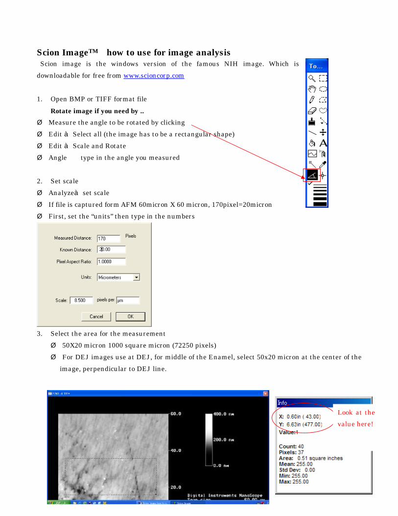
Scion ImageTM how to use for image analysis Scion image is the windows version of the famous NIH image. Which is downloadable for free from www.scioncorp.com 1. Open BMP or TIFF format file

Rotate image if you need by .. Ø Measure the angle to be rotated by clicking Ø Edit à Select all (the image has to be a rectangular shape) Ø Edit à Scale and Rotate Ø Angle type in the angle you measured 2. Set scale Ø Analyzeà set scale Ø If file is captured form AFM 60micron X 60 micron, 170pixel=20micron Ø First, set the “units” then type in the numbers

3. Select the area for the measurement Ø 50X20 micron 1000 square micron (72250 pixels) Ø For DEJ images use at DEJ, for middle of the Enamel, select 50x20 micron at the center of the

image, perpendicular to DEJ line.

Look at the value here!

4. Make a copy of selected area by File à Duplicate selection

5. If the image is in color, Option à Grayscale, then Edit àInvert 6. Modify the area if needed, with paintbrush and droppers etc.

7. Option àDensity Slice then move the LUT bar to turn your target area into red

8. Process à Make Binary Ø Process à Dilate to connect discontinuous objects and fills in holes Ø Process à Erode to separate objects that are touching and removes isolated pixels

Ø Process à Close to perform dilation operation followed by Erosion, which smoothes objects and fills in small holes.

9. Erase garbage by clicking eraser icon 10. Analyze Particle

Ø Analyze options to change the view of results (Area, length (perimeter))

1. Analyze -> Show results to view the current results 2. To copy the measurement to excel etc,

Edità copy measurement and paste to your destination. Kuniko Saeki September 2003