common functional principal components by michal benko ... · pdf filesubmitted to the annals...
TRANSCRIPT
Submitted to the Annals of Statistics
COMMON FUNCTIONAL PRINCIPAL COMPONENTS
By Michal Benko∗, Wolfgang Hardle and Alois Kneip
Humboldt-Universitat and Bonn Universitat
Functional principal component analysis (FPCA) based on the
Karhunen-Loeve decomposition has been successfully applied in many
applications, mainly for one sample problems. In this paper we con-
sider common functional principal components for two sample prob-
lems. Our research is motivated not only by the theoretical challenge
of this data situation but also by the actual question of dynamics
of implied volatility (IV) functions. For different maturities the log-
returns of IVs are samples of (smooth) random functions and the
methods proposed here study the similarities of their stochastic be-
havior. Firstly we present a new method for estimation of functional
principal components from discrete noisy data. Next we present the
two sample inference for FPCA and develop two sample theory. We
propose bootstrap tests for testing the equality of eigenvalues, eigen-
functions, and mean functions of two functional samples, illustrate
the test-properties by simulation study and apply the method to the
IV analysis.
1. Introduction. In many applications in biometrics, chemometrics, economet-
rics, etc., the data come from the observation of continuous phenomenons of time or
space and can be assumed to represent a sample of i.i.d. smooth random functions∗We gratefully acknowledge financial support by the Deutsche Forschungsgemeinschaft and the
Sonderforschungsbereich 649 “Okonomisches Risiko”.
AMS 2000 subject classifications: Primary 62H25,62G08; secondary 62P05
Keywords and phrases: Functional Principal Components, Nonparametric Regression, Bootstrap,
Two Sample Problem
1
2 M. BENKO, W. HARDLE AND A.KNEIP
X1(t), . . . , Xn(t) ∈ L2[0, 1]. Functional data analysis has received considerable at-
tention in the statistical literature during the last decade. In this context functional
principal component analysis (FPCA) has proved to be a key technique. An early
reference is Rao (1958), and important methodological contributions have been given
by various authors. Case studies, references, as well as methodological and algorith-
mical details can be found in the books by Ramsay & Silverman (2002), Ramsay &
Silverman (2005), or Ferraty and Vieu (2006).
The well-known Karhunen-Loeve (KL) expansion provides a basic tool to describe
the distribution of the random functions Xi and can be seen as the theoretical basis
of FPCA. For v, w ∈ L2[0, 1] let 〈v, w〉 =∫ 10 v(t)w(t)dt, and let ‖ · ‖= 〈·, ·〉1/2 denote
the usual L2-norm. With λ1 ≥ λ2 ≥ . . . and γ1, γ2, . . . denoting eigenvalues and
corresponding orthonormal eigenfunctions of the covariance operator Γ of Xi we obtain
Xi = µ +∞∑
r=1βriγr, i = 1, . . . , n, where µ = E(Xi) is the mean function and βri =
〈Xi−µ, γr〉 are (scalar) factor loadings with E(β2ri) = λr. Structure and dynamics of the
random functions can be assessed by analyzing the “functional principal components”
γr as well as the distribution of the factor loadings. For a given functional sample, the
unknown characteristics λr, γr are estimated by the eigenvalues and eigenfunctions of
the empirical covariance operator Γn of X1, . . . , Xn. Note that an eigenfunction γr is
identified (up to sign) only if the corresponding eigenvalue λr has multiplicity one.
This therefore establishes a necessary regularity condition for any inference based on
an estimated functional principal component γr in FPCA. Signs are arbitrary (γr and
βri can be replaced by −γr and −βri) and may be fixed by a suitable standardization.
More detailed discussion on this topic and precise assumptions can be found in section
2.
In many important applications a small number of functional principal components
COMMON FUNCTIONAL PC 3
will suffice to approximate the functions Xi with a high degree of accuracy. Indeed,
FPCA plays a much more central role in functional data analysis than its well-known
analogue in multivariate analysis. There are two major reasons. First, distributions on
function spaces are complex objects, and the Karhunen-Loeve expansion seems to be
the only practically feasible way to access their structure. Secondly, in multivariate
analysis a substantial interpretation of principal components is often difficult and has
to be based on vague arguments concerning the correlation of principal components
with original variables. Such a problem does not at all exists in the functional context,
where γ1(t), γ2(t), . . . are functions representing the major modes of variation of Xi(t)
over t.
In this paper we consider inference and tests of hypotheses on the structure of func-
tional principal components. Motivated by an application to implied volatility analysis
we will concentrate on the two sample case. A central point is the use of bootstrap
procedures. We will show that the bootstrap methodology can also be applied to func-
tional data.
In Section 2 we start by discussing one-sample inference for FPCA. Basic results
on asymptotic distributions have already been derived by Dauxois, Pousse & Romain
(1982) in situations where the functions are directly observable. Hall & Hosseini-Nasab
(2006) develop asymptotic Taylor expansions of estimated eigenfunctions in terms of
the difference Γn − Γ. Without deriving rigorous theoretical results, they also pro-
vide some qualitative arguments as well as simulation results motivating the use of
bootstrap in order to construct confidence regions for principal components.
In practice the functions of interest are often not directly observed but are regres-
sion curves which have to be reconstructed from discrete, noisy data. In this context
the standard approach is to first estimate individual functions nonparametrically (e.g.

4 M. BENKO, W. HARDLE AND A.KNEIP
by B-Splines) and then to determine principal components of the resulting estimated
empirical covariance operator – see, Besse & Ramsay (1986), Ramsay & Dalzell (1991),
among others. Approaches incorporating a smoothing step into the eigenanalysis have
been proposed by Rice & Silverman (1991), Pezzulli & Silverman (1993) or Silver-
man (1996). Robust estimation of principal component analysis has been considered
by Lacontore et.al. (1999). Yao, Muller &Wang (2005) and Hall, Muller & Wang
(2006) propose techniques based on nonparametric estimation of the covariance func-
tion E[(Xi(t) − µ(t))(Xi(s) − µ(s)] which can also be applied if there are only a few
scattered observations per curve.
Section 2.1 presents a new method for estimation of functional principal compo-
nents. It consists in an adaptation of a technique introduced by Kneip & Utikal (2001)
for the case of density functions. The key-idea is to represent the components of the
Karhunen-Loeve expansion in terms of an (L2) scalar-product matrix of the sample.
We investigate the asymptotic properties of the proposed method. It is shown that un-
der mild conditions the additional error caused by estimation from discrete, noisy data
is first-order asymptotically negligible, and inference may proceed ”as if” the functions
were directly observed. Generalizing the results of Dauxois, Pousse & Romain (1982),
we then present a theorem on the asymptotic distributions of the empirical eigenvalues
and eigenfunctions. The structure of the asymptotic expansion derived in the theorem
provides a basis to show consistency of bootstrap procedures.
Section 3 deals with two-sample inference. We consider two independent samples
of functions X(1)i n1
i=1 and X(2)i n2
i=1. The problem of interest is to test in how far
the distributions of these random functions coincide. The structure of the different
distributions in function space can be accessed by means of the respective Karhunen-
COMMON FUNCTIONAL PC 5
Loeve expansions
X(p)i = µ(p) +
∞∑
r=1
β(p)ri γ(p)
r , p = 1, 2.
Differences in the distribution of these random functions will correspond to differences
in the components of the respective KL expansions above. Without restriction one may
require that signs are such that 〈γ(1)1 , γ
(2)r 〉 ≥ 0. Two sample inference for FPCA in
general has not been considered in the literature so far. In Section 3 we define bootstrap
procedures for testing the equality of mean functions, eigenvalues, eigenfunctions, and
eigenspaces. Consistency of the bootstrap is derived in Section 3.1, while Section 3.2
contains a simulation study providing insight into the finite sample performance of
our tests.
It is of particular interest to compare the functional components characterizing the
two samples. If these factors are ”common”, this means γr := γ(1)r = γ
(2)r , then only
the factor loadings β(p)ri may vary across samples. This situation may be seen as a func-
tional generalization of the concept of ”common principal components” as introduced
by Flury (1988) in multivariate analysis. A weaker hypothesis may only require equal-
ity of the eigenspaces spanned by the first L ∈ IN functional principal components.
If for both samples the common L-dimensional eigenspaces suffice to approximate
the functions with high accuracy, then the distributions in function space are well
represented by a low dimensional factor model, and subsequent analysis may rely on
comparing the multivariate distributions of the random vectors (β(p)r1 , . . . , β
(p)rL )>.
The idea of ”common functional principal components” is of considerable impor-
tance in implied volatility (IV) dynamics. This application is discussed in detail in
Section 4. Implied volatility is obtained from the pricing model proposed by Black &
Scholes (1973) and is a key parameter for quoting options prices. Our aim is to con-
struct low dimensional factor models for the log-returns of the IV functions of options
6 M. BENKO, W. HARDLE AND A.KNEIP
Estimated Eigenfunctions, 1M
-2.00
-1.00
0.00
1.00
2.00
3.00
4.00
0.85 0.90 0.95 ATM 1.05
-2.00
-1.00
0.00
1.00
2.00
3.00
4.00
0.85 0.90 0.95 ATM 1.05
Estimated Eigenfunctions, 3M
-2.00
-1.00
0.00
1.00
2.00
3.00
4.00
0.85 0.90 0.95 ATM 1.05
-2.00
-1.00
0.00
1.00
2.00
3.00
4.00
0.85 0.90 0.95 ATM 1.05
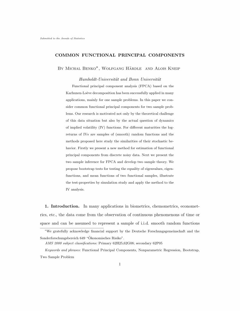
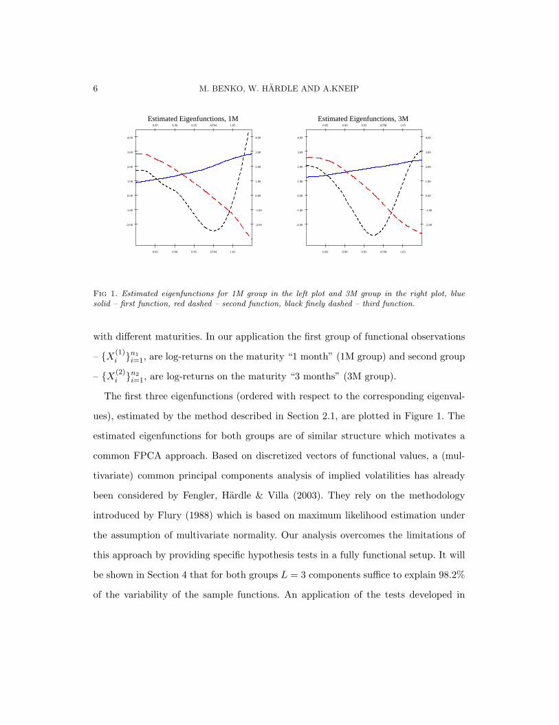
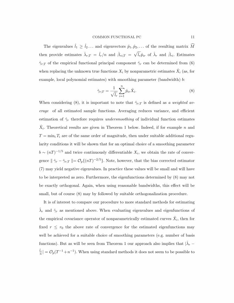
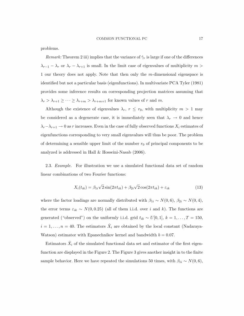
Fig 1. Estimated eigenfunctions for 1M group in the left plot and 3M group in the right plot, bluesolid – first function, red dashed – second function, black finely dashed – third function.
with different maturities. In our application the first group of functional observations
– X(1)i n1
i=1, are log-returns on the maturity “1 month” (1M group) and second group
– X(2)i n2
i=1, are log-returns on the maturity “3 months” (3M group).
The first three eigenfunctions (ordered with respect to the corresponding eigenval-
ues), estimated by the method described in Section 2.1, are plotted in Figure 1. The
estimated eigenfunctions for both groups are of similar structure which motivates a
common FPCA approach. Based on discretized vectors of functional values, a (mul-
tivariate) common principal components analysis of implied volatilities has already
been considered by Fengler, Hardle & Villa (2003). They rely on the methodology
introduced by Flury (1988) which is based on maximum likelihood estimation under
the assumption of multivariate normality. Our analysis overcomes the limitations of
this approach by providing specific hypothesis tests in a fully functional setup. It will
be shown in Section 4 that for both groups L = 3 components suffice to explain 98.2%
of the variability of the sample functions. An application of the tests developed in

COMMON FUNCTIONAL PC 7
Section 3 does not reject the equality of the corresponding eigenspaces.
2. Functional Principal Components and one sample inference. In this
section we will focus on one sample of i.i.d. smooth random functions X1, . . . , Xn
∈ L2[0, 1]. We will assume a well-defined mean function µ = E(Xi) as well as the
existence of a continuous covariance function σ(t, s) = E[Xi(t)−µ(t)Xi(s)−µ(s)].Then E(‖Xi−µ‖2) =
∫σ(t, t)dt < ∞, and the covariance operator Γ of Xi is given by
(Γv)(t) =∫
σ(t, s)v(s)ds, v ∈ L2[0, 1].
The Karhunen-Loeve decomposition provides a basic tool to describe the distri-
bution of the random functions Xi. With λ1 ≥ λ2 ≥ . . . and γ1, γ2, . . . denoting
eigenvalues and a corresponding complete orthonormal basis of eigenfunctions of Γ we
obtain
Xi = µ +∞∑
r=1
βriγr, i = 1, . . . , n, (1)
where βri = 〈Xi − µ, γr〉 are uncorrelated (scalar) factor loadings with E(βri) = 0,
E(β2ri) = λr, and E(βriβki) = 0 for r 6= k. Structure and dynamics of the random
functions can be assessed by analyzing the ”functional principal components” γr as
well as the distribution of the factor loadings.
A discussion of basic properties of (1) can, for example, be found in Gihman and
Skorohod (1973). Under our assumptions, the infinite sums in (1) converge with prob-
ability 1, and∑∞
r=1 λr = E(‖Xi − µ‖2) < ∞. Smoothness of Xi carries over to a
corresponding degree of smoothness of σ(t, s) and γr. If, with probability 1, Xi(t) is
twice continuously differentiable, then σ as well as γr are also twice continuously dif-
ferentiable. The particular case of a Gaussian random function Xi implies that the βri
are independent N(0, λr)-distributed random variables.
8 M. BENKO, W. HARDLE AND A.KNEIP
An important property of (1) consists in the known fact that the first L principal
components provide a “best basis” for approximating the sample functions in terms
of the integrated square error, see Ramsay & Silverman (2005), section 6.2.3, among
others. For any choice of L orthonormal basis functions v1, . . . , vL the mean integrated
square error:
ρ(v1, . . . , vL) = E(‖ Xi − µ−L∑
r=1
〈Xi − µ, vr〉vr ‖2) (2)
is minimized by vr = γr.
2.1. Estimation of Functional Principal Components. For a given sample an em-
pirical analog of (1) can be constructed by using eigenvalues λ1 ≥ λ2 ≥ . . . and
orthonormal eigenfunctions γ1, γ2, . . . of the empirical covariance operator Γn, where
(Γnv)(t) =∫
σ(t, s)v(s)ds
with X = n−1n∑
i=1Xi and σ(t, s) = n−1
n∑i=1Xi(t) − X(t)Xi(s) − X(s) denoting
sample mean and covariance function. Then
Xi = X +n∑
r=1
βriγr, i = 1, . . . , n, (3)
where βri = 〈γr, Xi− X〉. We necessarily obtain n−1∑
i βri = 0, n−1∑
i βriβsi = 0 for
r 6= s, and n−1∑
i β2ri = λr.
Analysis will have to concentrate on the leading principal components explaining
the major part of the variance. In the following we will assume that λ1 > λ2 > · · · >λr0 > λr0+1, where r0 denotes the maximal number of components to be considered.
For all r = 1, . . . , r0 the corresponding eigenfunction γr then is uniquely defined up
to sign. Signs are arbitrary, decompositions (1) or (3) may just as well be written in
terms of −γr,−βri or −γr,−βri, and any suitable standardization may be applied by
the statistician. In order to ensure that γr may be viewed as an estimator of γr rather
COMMON FUNCTIONAL PC 9
than of −γr we will in the following only assume that signs are such that 〈γr, γr〉 ≥ 0.
More generally, any subsequent statement concerning differences of two eigenfunctions
will be based on the condition of a non-negative inner product. This does not impose
any restriction and will go without saying.
The results of Dauxois, Pousse & Romain (1982) imply that under regularity condi-
tions, ‖ γr−γr ‖= Op(n−1/2), |λr−λr| = Op(n−1/2), as well as |βri−βri| = Op(n−1/2)
for all r ≤ r0.
However, in practice, the sample functions Xi are often not directly observed, but
have to be reconstructed from noisy observations Yij at discrete design points tik:
Yik = Xi(tik) + εik, k = 1, . . . , Ti, (4)
where εik are independent noise terms with E(εik) = 0, Var(εik) = σ2i .
Our approach for estimating principal components is motivated by the well known
duality relation between row and column spaces of a data matrix, see Hardle, & Simar
(2003) chapter 8, among others. In a first step this approach relies on estimating the
elements of the matrix:
Mlk = 〈Xl − X, Xk − X〉, l, k = 1, . . . , n. (5)
Some simple linear algebra shows that all nonzero eigenvalues λ1 ≥ λ2 . . . of Γn and
l1 ≥ l2 . . . of M are related by λr = lr/n, r = 1, 2, . . . . When using the correspond-
ing orthonormal eigenvectors p1, p2, . . . of M , the empirical scores βri as well as the
empirical eigenfunctions γr are obtained by βri =√
lrpir and
γr =1√lr
n∑
i=1
pir
(Xi − X
)=
1√lr
n∑
i=1
pirXi. (6)
The elements of M are functionals which can be estimated with asympotically neg-
ligible bias and a parametric rate of convergence T−1/2i . If the data in (4) is generated
10 M. BENKO, W. HARDLE AND A.KNEIP
from a balanced, equidistant design, then it is easily seen that for i 6= j this rate of
convergence is achieved by the estimator:
Mij = T−1T∑
k=1
(Yik − Y·k)(Yjk − Y·k), i 6= j,
and
Mii = T−1T∑
k=1
(Yik − Y·k)2 − σ2i .
Where σ2i denotes some nonparametric estimator of variance and Y·k = n−1
∑nj=1 Yjk.
In the case of a random design some adjustment is necessary: Define the ordered
sample ti(1) ≤ ti(2) ≤ · · · ≤ ti(Ti) of design points, and for j = 1, . . . , Ti let Yi(j) denote
the observation belonging to ti(j). With ti(0) = −ti(1) and ti(Ti+1) = 2− ti(Ti) set
χi(t) =Ti∑
j=1
Yi(j)I
(t ∈
[ti(j−1) + ti(j)
2,ti(j) + ti(j+1)
2
]), t ∈ [0, 1],
where I(·) denotes the indicator function, and for i 6= j define the estimate of Mij by
Mij =∫ 1
0χi(t)− χ(t) χj(t)− χ(t) dt,
where χ(t) = n−1∑n
i=1 χi(t). Finally, by redefining ti(1) = −ti(2) and ti(Ti+1) =
2 − ti(Ti), set χ∗i (t) =∑Ti
j=2 Yi(j−1)I(t ∈ [ ti(j−1)+ti(j)
2 ,ti(j)+ti(j+1)
2 ]), t ∈ [0, 1]. Then
construct estimators of the diagonal terms Mii by
Mii =∫ 1
0χi(t)− χ(t) χ∗i (t)− χ(t) dt. (7)
The aim of using the estimator (7) for the diagonal terms is to avoid the additional
bias implied by Eε(Y 2ik) = Xi(tij)2 + σ2
i . Here Eε denotes conditional expectation
given tij , Xi. Alternatively we can construct a bias corrected estimator using some
nonparametric estimation of variance σ2i , e.g. the difference based model-free variance
estimators studied in Hall, Kay & Titterington (1990) can be employed.
COMMON FUNCTIONAL PC 11
The eigenvalues l1 ≥ l2 . . . and eigenvectors p1, p2, . . . of the resulting matrix M
then provide estimates λr;T = lr/n and βri;T =√
lrpir of λr and βri. Estimates
γr;T of the empirical functional principal component γr can be determined from (6)
when replacing the unknown true functions Xi by nonparametric estimates Xi (as, for
example, local polynomial estimates) with smoothing parameter (bandwidth) b:
γr;T =1√lr
n∑
i=1
pirXi. (8)
When considering (8), it is important to note that γr;T is defined as a weighted av-
erage of all estimated sample functions. Averaging reduces variance, and efficient
estimation of γr therefore requires undersmoothing of individual function estimates
Xi. Theoretical results are given in Theorem 1 below. Indeed, if for example n and
T = mini Ti are of the same order of magnitude, then under suitable additional regu-
larity conditions it will be shown that for an optimal choice of a smoothing parameter
b ∼ (nT )−1/5 and twice continuously differentiable Xi, we obtain the rate of conver-
gence ‖ γr − γr;T ‖= Op(nT )−2/5. Note, however, that the bias corrected estimator
(7) may yield negative eigenvalues. In practice these values will be small and will have
to be interpreted as zero. Furthermore, the eigenfunctions determined by (8) may not
be exactly orthogonal. Again, when using reasonable bandwidths, this effect will be
small, but of course (8) may by followed by suitable orthogonalization procedure.
It is of interest to compare our procedure to more standard methods for estimating
λr and γr as mentioned above. When evaluating eigenvalues and eigenfunctions of
the empirical covariance operator of nonparametrically estimated curves Xi, then for
fixed r ≤ r0 the above rate of convergence for the estimated eigenfunctions may
well be achieved for a suitable choice of smoothing parameters (e.g. number of basis
functions). But as will be seen from Theorem 1 our approach also implies that |λr −lrn | = Op(T−1 +n−1). When using standard methods it does not seem to be possible to
12 M. BENKO, W. HARDLE AND A.KNEIP
obtain a corresponding rate of convergence, since any smoothing bias |E[Xi(t)]−Xi(t)|will invariably affect the quality of the corresponding estimate of λr.
We want to emphasize that any finite sample interpretation will require that T
be sufficiently large such that our nonparametric reconstructions of individual curves
can be assumed to possess a fairly small bias. The above arguments do not apply to
extremely sparse designs with very few observations per curve (see Hall, Muller &
Wang (2006) for an FPCA methodolgy focusing on sparse data).
Note that in addition to (8) our final estimate of the empirical mean function µ = X
will be given by µT = n−1∑
i Xi. A straightforward approach to determine a suitable
bandwidth b consists in a ”leave-one-individual-out” cross-validation. For the maximal
number r0 of components to be considered let µT,−i and γr;T,−i, r = 1, . . . , r0, denote
the estimates of µ and γr obtained from the data (Ylj , tlj), l = 1, . . . , i−1, i+1, . . . , n,
j = 1, . . . , Tk. By (8) these estimates depend on b, and one may approximate an
optimal smoothing parameter by minimizing
∑
i
∑
j
Yij − µT,−i(tij)−
r0∑
r=1
ϑriγr;T,−i(tij)
2
over b, where ϑri denote ordinary least squares estimates of βri. A more sophisticated
version of this method may even allow to select different bandwidths br when estimat-
ing different functional principal components by (8). Although, under certain regular-
ity conditions, the same qualitative rates of convergence hold for any arbitrary fixed
r ≤ r0, the quality of estimates decreases when r becomes large. Due to 〈γs, γr〉 = 0
for s < r, the number of zero crossings, peaks and valleys of γr has to increase with r.
Hence, in tendency γr will be less and less smooth as r increases. At the same time,
λr → 0 which means that for large r the r-th eigenfunctions will only possess a very
small influence on the structure of Xi. This in turn means that the relative importance

COMMON FUNCTIONAL PC 13
of the error terms εik in (4) on the structure of γr;T will increase with r.
2.2. One sample inference. Clearly, in the framework described by (1) - (4) we
are faced with two sources of variability of estimated functional principal components.
Due to sampling variation γr will differ from the true component γr, and due to (4)
there will exist an additional estimation error when approximating γr by γr;T .
The following theorems quantify the order of magnitude of these different types of
error. Our theoretical results are based on the following assumptions on the structure
of the random functions Xi. IN will denote the set of all natural numbers 1, 2, . . .
(0 6∈ IN).
Assumption 1.
X1, . . . , Xn ∈ L2[0, 1] is an i.i.d. sample of random functions with mean µ and contin-
uous covariance function σ(t, s), and (1) holds for a system of eigenfunctions satisfying
sups∈IN supt∈[0,1] |γs(t)| < ∞. Furthermore,∑∞
r=1
∑∞s=1 E[β2
riβ2si] < ∞ and
∑∞q=1
∑∞s=1 E[β2
riβqiβsi] < ∞ for all r ∈ IN .
Recall that E[βri] = 0 and E[βriβsi] = 0 for r 6= s. Note that the assumption on
the factor loadings is necessarily fulfilled if Xi are Gaussian random functions. Then
βri and βsi are independent for r 6= s, all moments of moments βri are finite, and
hence E[β2riβqiβsi] = 0 for q 6= s as well as E[β2
riβ2si] = λrλs for r 6= s, see Gihman and
Skorohod (1973).
We need some further assumptions concerning smoothness of Xi and the structure
of the discrete model (4).
Assumption 2.
a) Xi is a.s. twice continuously differentiable. There exists a constant D1 < ∞ such
that the derivatives are bounded by supt E[X′i(t)
4] ≤ D1 as well as supt E[X′′i (t)4] ≤
D1.

14 M. BENKO, W. HARDLE AND A.KNEIP
b) The design points tik, i = 1, . . . , n, k = 1, . . . , Ti are i.i.d. random variables which
are independent of Xi and εik. The corresponding design density f is continuous
on [0, 1] and satisfies inft∈[0,1] f(t) > 0.
c) For any i the error terms εik are i.i.d. zero mean random variables with Var(εik) =
σ2i . Furthermore, εik is independent of Xi, and there exists a constant D2 such
that E(ε8ik) < D2 for all i, k.
d) The estimates Xi used in (8) are determined by either a local linear or a Nadaraya-
Watson kernel estimator with smoothing parameter b and kernel function K. K
is a continuous probability density which is symmetric at 0.
The following theorems provide asymptotic results as n, T →∞, where T = minni=1Ti.
Theorem 1: In addition to Assumptions 1 and 2 assume that infs 6=r |λr − λs| > 0
holds for some r = 1, 2, . . . . Then
i) n−1∑n
i=1(βri − βri;T )2 = Op(T−1) and
|λr − lrn| = Op(T−1 + n−1). (9)
ii) If additionally b → 0 and (Tb)−1 → 0 as n, T →∞, then for all t ∈ [0, 1]
|γr(t)− γr;T (t)| = Opb2 + (nTb)−1/2 + (Tb1/2)−1 + n−1. (10)
A proof is given in the appendix.
Theorem 2: Under Assumption 1 we obtain:
i) For all t ∈ [0, 1]
√nX(t)− µ(t) =
∑r
1√n
n∑
i=1
βri
γr(t)
L→ N
(0,
∑r
λrγr(t)2)
,
COMMON FUNCTIONAL PC 15
If, furthermore, λr−1 > λr > λr+1 holds for some fixed r ∈ 1, 2, . . . , then
ii)
√n(λr − λr) =
1√n
n∑
i=1
(β2
ri − λr
)+Op(n−1/2) L→ N(0,Λr), (11)
where Λr = E[(β2ri − λr)2],
iii) and for all t ∈ [0, 1]
γr(t)− γr(t) =∑
s 6=r
1
n(λr − λs)
n∑
i=1
βsiβri
γs(t) + Rr(t), where ‖Rr‖ = Op(n−1).
(12)
Moreover,
√n
∑
s 6=r
1
n(λr − λs)
n∑
i=1
βsiβri
γs(t)
L→ N
0,
∑
q 6=r
∑
s 6=r
E[β2riβqiβsi]
(λq − λr)(λs − λr)γq(t)γs(t)
A proof can be found in the appendix. The theorem provides a generalization of the
results of Dauxois, Pousse & Romain (1982) who derive explicit asymptotic distribu-
tions by assuming Gaussian random functions Xi. Note that in this case Λr = 2λ2r,
and∑
q 6=r
∑s 6=r
E[β2riβqiβsi]
(λq−λr)(λs−λr)γq(t)γs(t) =∑
s6=rλrλs
(λs−λr)2γs(t)2.
When evaluating the bandwidth depend terms in (10), best rates of convergence
|γr(t)− γr;T (t)| = OP ((nT )−2/5 + T−4/5 + n−1) are achieved when choosing an under-
smoothing bandwidth b ∼ max(nT )−1/5, T−2/5. Theoretical work in functional data
analysis is usually based on the implicit assumption that the additional error due to (4)
is negligible, and that one can proceed “as if” the functions Xi were directly observed.
In view of Theorems 1 and 2 this approach is justified in the following situations:
1) T is much larger than n, i.e. n/T 4/5 → 0, and the smoothing parameter b in (8)
is of order T−1/5 (optimal smoothing of individual functions).
16 M. BENKO, W. HARDLE AND A.KNEIP
2) An undersmoothing bandwidth b ∼ max(nT )−1/5, T−2/5 is used and n/T 8/5 →0. This means that T may be smaller than n, but T must be at least of order of
magnitude larger than n5/8.
In both cases 1) and 2) the above theorems imply that |λr − lrn | = Op(|λr − λr|) as
well as ‖γr − γr;T ‖ = Op(‖γr − γr‖). Inference about functional principal components
will then be first order equivalent to an inference based on known functions Xi.
In such situations Theorem 2 suggests bootstrap procedures as tools for one sam-
ple inference. For example, the distribution of ‖γr − γr‖ may by approximated by
the bootstrap distribution of ‖γ∗r − γr‖, where γ∗r are estimates to be obtained from
i.i.d. bootstrap resamples X∗1 , X∗
2 , . . . , X∗n of X1, X2, . . . , Xn. This means that X∗
1 =
Xi1 , . . . , X∗n = Xin for some indices i1, . . . , in drawn independently and with replace-
ment from 1, . . . , n and, in practice, γ∗r may thus be approximated from correspond-
ing discrete data (Yi1j , ti1j)j=1,....Ti1, . . . , (Yinj , tinj)j=1,....Tin
. The additional error is
negligible if either 1) or 2) are satisfied.
One may wonder about the validity of such a bootstrap. Functions are complex
objects and there is no established result in bootstrap theory which readily generalizes
to samples of random functions. But by (1) i.i.d. bootstrap resamples X∗i i=1,...,n may
be equivalently represented by corresponding i.i.d. resamples β∗1i, β∗2i, . . . i=1,...,n of
factor loadings. Standard multivariate bootstrap theorems imply that for any q ∈ IN
the distribution of moments of the random vectors (β1i, . . . , βqi) may be consistently
approximated by the bootstrap distribution of corresponding moments of (β∗1i, . . . , β∗qi).
Together with some straightforward limit arguments as q → ∞, the structure of the
first order terms in the asymptotic expansions (11) and (12) then allows to establish
consistency of the functional bootstrap. These arguments will be made precise in the
proof of Theorem 3 below, which concerns related bootstrap statistics in two sample
COMMON FUNCTIONAL PC 17
problems.
Remark: Theorem 2 iii) implies that the variance of γr is large if one of the differences
λr−1 − λr or λr − λr+1 is small. In the limit case of eigenvalues of multiplicity m >
1 our theory does not apply. Note that then only the m-dimensional eigenspace is
identified but not a particular basis (eigenfunctions). In multivariate PCA Tyler (1981)
provides some inference results on corresponding projection matrices assuming that
λr > λr+1 ≥ · · · ≥ λr+m > λr+m+1 for known values of r and m.
Although the existence of eigenvalues λr, r ≤ r0, with multiplicity m > 1 may
be considered as a degenerate case, it is immediately seen that λr → 0 and hence
λr−λr+1 → 0 as r increases. Even in the case of fully observed functions Xi estimates of
eigenfunctions corresponding to very small eigenvalues will thus be poor. The problem
of determining a sensible upper limit of the number r0 of principal components to be
analyzed is addressed in Hall & Hosseini-Nasab (2006).
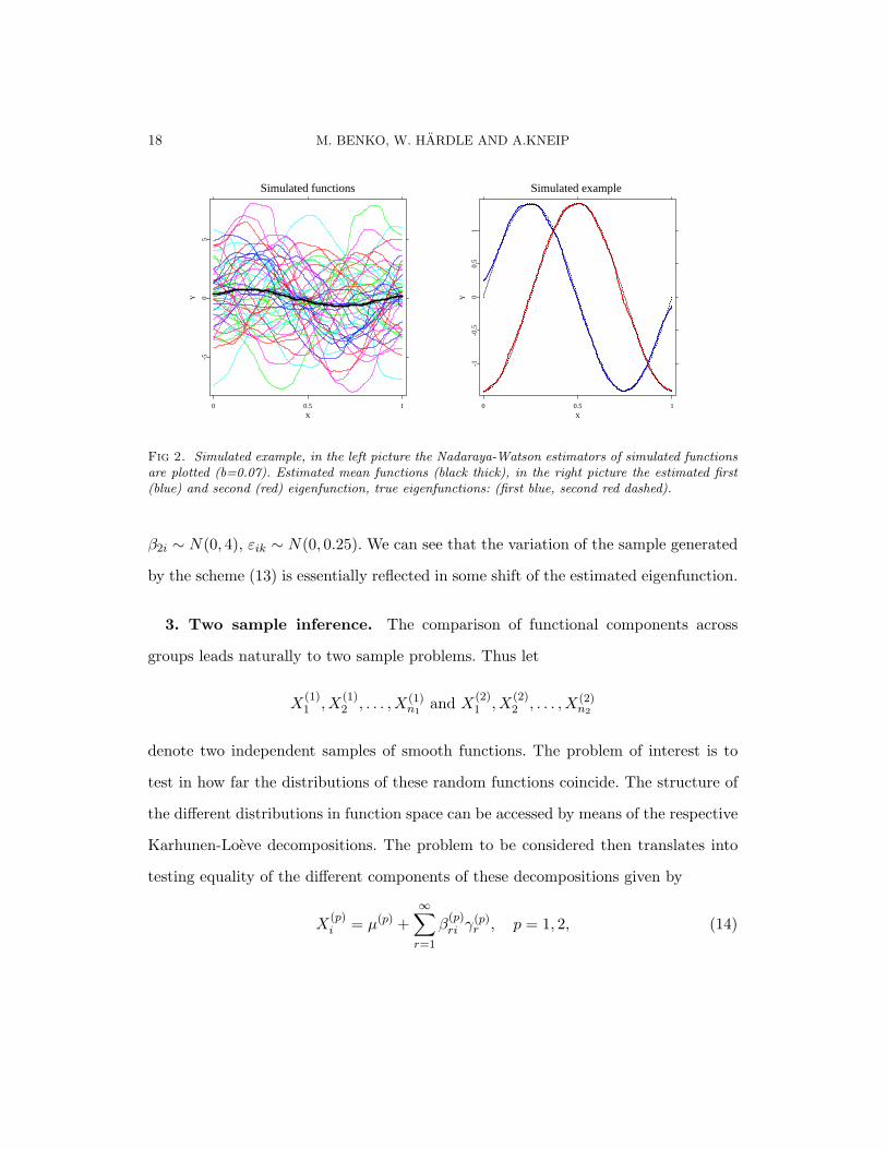
2.3. Example. For illustration we use a simulated functional data set of random
linear combinations of two Fourier functions:
Xi(tik) = β1i
√2 sin(2πtik) + β2i
√2 cos(2πtik) + εik (13)
where the factor loadings are normally distributed with β1i ∼ N(0, 6), β2i ∼ N(0, 4),
the error terms εik ∼ N(0, 0.25) (all of them i.i.d. over i and k). The functions are
generated (“observed”) on the uniformly i.i.d. grid tik ∼ U [0, 1], k = 1, . . . , T = 150,
i = 1, . . . , n = 40. The estimators Xi are obtained by the local constant (Nadaraya-
Watson) estimator with Epanechnikov kernel and bandwidth b = 0.07.
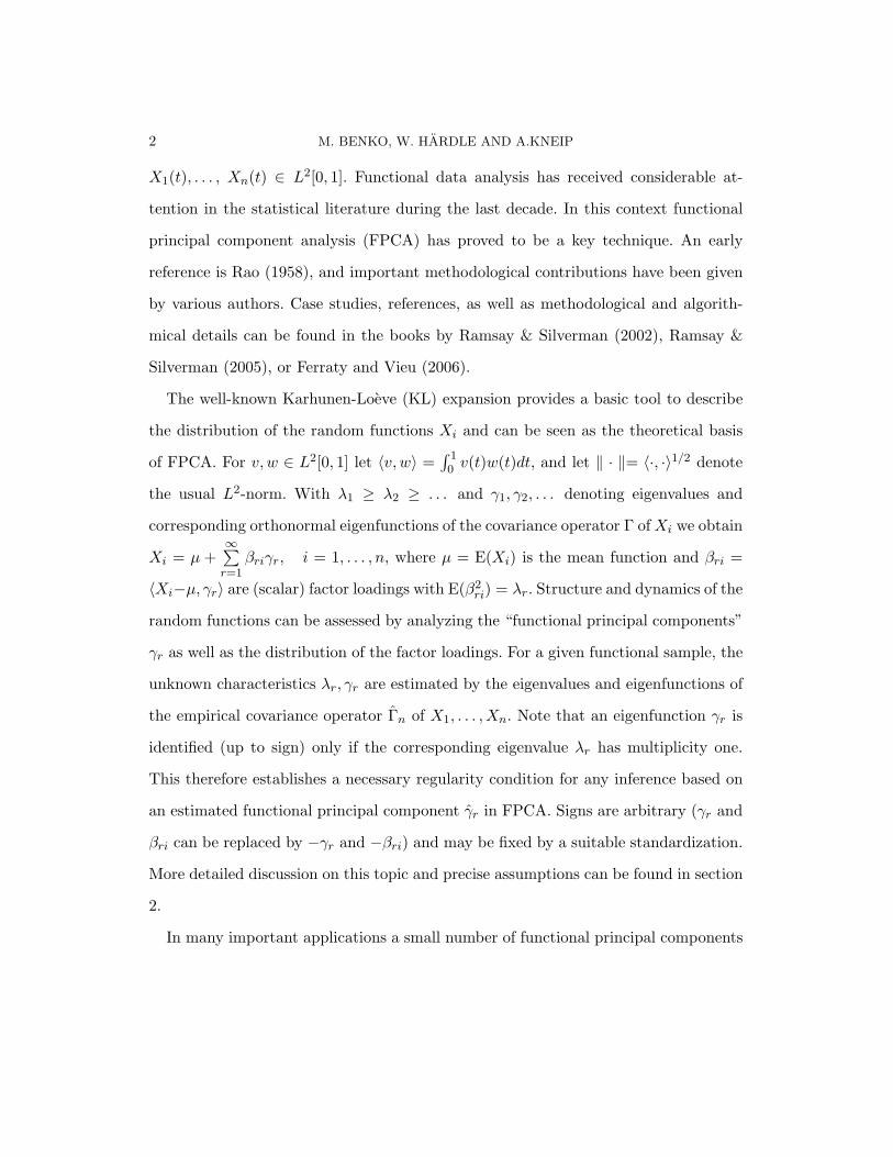
Estimators Xi of the simulated functional data set and estimator of the first eigen-
function are displayed in the Figure 2. The Figure 3 gives another insight in to the finite
sample behavior. Here we have repeated the simulations 50 times, with β1i ∼ N(0, 6),
18 M. BENKO, W. HARDLE AND A.KNEIP
Simulated functions
0 0.5 1
X
-50
5
YSimulated example
0 0.5 1
X
-1-0
.50
0.5
1
YFig 2. Simulated example, in the left picture the Nadaraya-Watson estimators of simulated functionsare plotted (b=0.07). Estimated mean functions (black thick), in the right picture the estimated first(blue) and second (red) eigenfunction, true eigenfunctions: (first blue, second red dashed).
β2i ∼ N(0, 4), εik ∼ N(0, 0.25). We can see that the variation of the sample generated
by the scheme (13) is essentially reflected in some shift of the estimated eigenfunction.
3. Two sample inference. The comparison of functional components across
groups leads naturally to two sample problems. Thus let
X(1)1 , X
(1)2 , . . . , X(1)
n1and X
(2)1 , X
(2)2 , . . . , X(2)
n2
denote two independent samples of smooth functions. The problem of interest is to
test in how far the distributions of these random functions coincide. The structure of
the different distributions in function space can be accessed by means of the respective
Karhunen-Loeve decompositions. The problem to be considered then translates into
testing equality of the different components of these decompositions given by
X(p)i = µ(p) +
∞∑
r=1
β(p)ri γ(p)
r , p = 1, 2, (14)

COMMON FUNCTIONAL PC 19
Monte Carlo Simulation
0 0.5 1X
-1.5
-1-0
.50
0.5
1
Y
Fig 3. Monte Carlo Simulation, 50 replications, thin lines are estimated first eigenfunctions, the boldblack line is the true eigenfunction
where again γ(p)r are the eigenfunctions of the respective covariance operator Γ(p)
corresponding to the eigenvalues λ(p)1 = E(β(p)
1i )2 ≥ λ(p)2 = E(β(p)
2i )2 ≥ . . . . We
will again suppose that λ(p)r−1 > λ
(p)r > λ
(p)r+1, p = 1, 2, for all r ≤ r0 components to be
considered. Without restriction we will additionally assume that signs are such that
〈γ(1)r , γ
(2)r 〉 ≥ 0 as well as 〈γ(1)
r , γ(2)r 〉 ≥ 0.
It is of great interest to detect possible variations in the functional components char-
acterizing the two samples in (14). Significant difference may give rise to substantial
interpretation. Important hypotheses to be considered thus are:
H01 : µ(1) = µ(2) and H02,r : γ(1)r = γ(2)
r , r ≤ r0
Hypothesis H02,r is of particular importance. Then γ(1)r = γ
(2)r and only the factor
loadings βri may vary across samples. If, for example, H02,r is accepted one may
additionally want to test hypotheses about the distributions of β(p)ri , p = 1, 2. Recall
that necessarily Eβ(p)ri = 0, Eβ(p)
ri 2 = λ(p)r , and β
(p)si is uncorrelated with β
(p)ri if

20 M. BENKO, W. HARDLE AND A.KNEIP
r 6= s. If the X(p)i are Gaussian random variables, the β
(p)ri are independent N(0, λr)
random variables. A natural hypothesis to be tested then refers to the equality of
variances:
H03,r : λ(1)r = λ(2)
r , r = 1, 2, . . .
Let µ(p)(t) = 1np
∑i X
(p)i (t), and let λ
(p)1 ≥ λ
(p)2 ≥ . . . and γ
(p)1 , γ
(p)2 ≥ . . . denote
eigenvalues and corresponding eigenfunctions of the empirical covariance operator Γ(p)np
of X(p)1 , X
(p)2 (t), . . . , X
(p)np . The following test statistics are defined in terms of µ(p), λ
(p)r
and γ(p)r . As discussed in the proceeding section, all curves in both samples are usually
not directly observed, but have to be reconstructed from noisy observations according
to (4). In this situation, the “true” empirical eigenvalues and eigenfunctions have to
be replaced by their discrete sample estimates. Bootstrap estimates are obtained by
resampling the observations corresponding to the unknown curves X(p)i . As discussed
in Section 2.2, the validity of our test procedures is then based on the assumption
that T is sufficiently large such that the additional estimation error is asymptotically
negligible.
Our tests of the hypotheses H01 ,H02,r and H03,r rely on the statistics
D1def= ‖µ(1) − µ(2)‖2,
D2,rdef= ‖γ(1)
r − γ(2)r ‖2,
D3,rdef= |λ(1)
r − λ(2)r |2.
The respective null-hypothesis has to be rejected if D1 ≥ ∆1;1−α, D2,r ≥ ∆2,r;1−α or
D3,r ≥ ∆3,r;1−α, where ∆1;1−α, ∆2,r;1−α and ∆3,r;1−α denote the critical values of the
COMMON FUNCTIONAL PC 21
distributions of
∆1def= ‖µ(1) − µ(1) − (µ(2) − µ(2))‖2,
∆2,rdef= ‖γ(1)
r − γ(1)r − (γ(2)
r − γ(2)r )‖2,
∆3,rdef= |λ(1)
r − λ(1)r − (λ(2)
r − λ(2)r )|2.
Of course, the distributions of the different ∆’s cannot be accessed directly, since
they depend on the unknown true population mean, eigenvalues and eigenfunctions.
However, it will be shown below that these distributions and hence their critical values
are approximated by the bootstrap distribution of
∆∗1
def= ‖µ(1)∗ − µ(1) − (µ(2)∗ − µ(2))‖2,
∆∗2,r
def= ‖γ(1)∗r − γ(1)
r − (γ(2)∗r − γ(2)
r )‖2,
∆∗3,r
def= |λ(1)∗r − λ(1)
r − (λ(2)∗r − λ(2)
r )|2.
where µ(1)∗, γ(1)∗r , λ
(1)∗r as well as µ(2)∗, γ
(2)∗r , λ
(2)∗r are estimates to be obtained from
independent bootstrap samples X1∗1 (t), X1∗
2 (t), . . . , X1∗n1
(t) as well as X2∗1 (t), X2∗
2 (t),
. . . , X2∗n2
(t).
This test procedure is motivated by the following insights:
1) Under each of our null-hypotheses the respective test statistics D is equal to the
corresponding ∆. The test will thus asymptotically possess the correct level: P (D >
∆1−α) ≈ α.
2) If the null hypothesis is false, then D 6= ∆. Compared to the distribution of ∆
the distribution of D is shifted by the difference in the true means, eigenfunctions, or
eigenvalues. In tendency D will be larger than ∆1−α.
Let 1 < L ≤ r0. Even if for r ≤ L the equality of eigenfunctions is rejected, we may
be interested in the question whether at least the L-dimensional eigenspaces generated

22 M. BENKO, W. HARDLE AND A.KNEIP
by the first L eigenfunctions are identical. Therefore, let E(1)L as well as E(2)
L denote
the L-dimensional linear function spaces generated by the eigenfunctions γ(1)1 , . . . , γ
(1)L
and γ(2)1 , . . . , γ
(2)L , respectively. We then aim to test the null hypothesis:
H04,L : E(1)L = E(2)
L .
Of course, H04,L corresponds to the hypothesis that the operators projecting into E(1)L
and E(2)L are identical. This in turn translates into the condition that
L∑
r=1
γ(1)r (t)γ(1)
r (s) =L∑
r=1
γ(2)r (t)γ(2)
r (s) for all t, s ∈ [0, 1].
Similar to above, a suitable test statistics is given by
D4,Ldef=
∫ ∫ L∑
r=1
γ(1)r (t)γ(1)
r (s)−L∑
r=1
γ(2)r (t)γ(2)
r (s)
2
dtds
and the null hypothesis is rejected if D4,L ≥ ∆4,L;1−α, where ∆4,L;1−α denotes the
critical value of the distribution of
∆4,Ldef=
∫ ∫ [L∑
r=1
γ(1)r (t)γ(1)
r (s)− γ(1)r (t)γ(1)
r (s)
−L∑
r=1
γ(2)r (t)γ(2)
r (s)− γ(2)r (t)γ(2)
r (s)]2
dtds.
The distribution of ∆4,L and hence its critical values are approximated by the
bootstrap distribution of
∆∗4,L
def=∫ ∫ [
L∑
r=1
γ(1)∗r (t)γ(1)∗
r (s)− γ(1)r (t)γ(1)
r (s)
−L∑
r=1
γ(2)∗r (t)γ(2)∗
r (s)− γ(2)r (t)γ(2)
r (s)]2
dtds.
It will be shown in Theorem 3 below that under the null hypothesis as well as under the
alternative the distributions of n∆1, n∆2,r, n∆3,r, n∆4,L converge to continuous limit
distributions which can be consistently approximated by the bootstrap distributions
of n∆∗1, n∆∗
2,r, n∆∗3,r, n∆∗
4,L.

COMMON FUNCTIONAL PC 23
3.1. Theoretical Results. Let n = (n1 +n2)/2. We will assume that asymptotically
n1 = n · q1 and n2 = n · q2 for some fixed proportions q1 and q2. We will then study
the asymptotic behavior of our statistics as n →∞.
We will use X1 = X(1)1 , . . . , X
(1)n1 and X2 = X(2)
1 , . . . , X(2)n2 to denote the observed
samples of random functions.
Theorem 3: Assume that X(1)1 , . . . , X
(1)n1 and X(2)
1 , . . . , X(2)n2 are two indepen-
dent samples of random functions each of which satisfies Assumption 1. As n →∞ we
then obtain:
i) There exists a non-degenerated, continuous probability distribution F1 such that
n∆1L→ F1, and for any δ > 0,
|P (n∆1 ≥ δ)− P (n∆∗1 ≥ δ| X1,X2) | = Op(1).
ii) If, furthermore, λ(1)r−1 > λ
(1)r > λ
(1)r+1 and λ
(2)r−1 > λ
(2)r > λ
(2)r+1 hold for some fixed
r = 1, 2, . . . , there exist a non-degenerated, continuous probability distributions
Fk,r such that n∆k,rL→ Fk,r, k = 2, 3, and for any δ > 0,
|P (n∆k,r ≥ δ)− P(n∆∗
k,r ≥ δ| X1,X2
) | = Op(1), k = 2, 3.
iii) If λ(1)r > λ
(1)r+1 > 0 and λ
(2)r > λ
(2)r+1 > 0 hold for all r = 1, . . . , L, there exists
a non-degenerated, continuous probability distribution F4,L such that n∆4,LL→
F4,L, and for any δ > 0,
|P (n∆4,L ≥ δ)− P(n∆∗
4,L ≥ δ| X1,X2
) | = Op(1).
The structures of the distributions F1, F2,r, F3,r, F4,L are derived in the proof of
the theorem which can be found in the appendix. They are obtained as limits of
distributions of quadratic forms.
24 M. BENKO, W. HARDLE AND A.KNEIP
3.2. Simulation study. In this paragraph we illustrate the finite behavior of the
proposed test. We make use of the findings of the Example 2.3 and focus here on the
test of common eigenfunctions. Looking at the Figure 3 we observe that the error of
the estimation of the eigenfunctions simulated by (13) is manifested by some shift of
the estimated eigenfunctions. This motivates the basic simulation-setup (setup “a”),
where the first sample is generated by the random combination of orthonormalized
sine and cosine functions (Fourier functions) and the second sample is generated by
the random combination of the same but shifted factor functions:
X(1)i (tik) = β
(1)1i
√2 sin(2πtik) + β
(1)2i
√2 cos(2πtik)
X(2)i (tik) = β
(2)1i
√2 sin2π(tik + δ)+ β
(2)2i
√2 cos2π(tik + δ).
The factor loadings are i.i.d. random variables with β(p)1i ∼ N(0, λ(p)
1 ) and β(p)2i ∼
N(0, λ(p)2 ). The functions are generated on the equidistant grid tik = tk = k/T, k =
1, . . . T = 100, i = 1, . . . , n = 70. For the presentation of results in the Table 1, we use
the following notation: “a) λ(1)1 , λ
(1)2 , λ
(2)2 , λ
(2)2 ”. The shift parameter δ is changing
from 0 to 0.25 with the step 0.05. It should be mentioned that the shift δ = 0 yields
the simulation of level and setup with shift “δ = 0.25” yields the simulation of the
alternative, where the two factor functions are exchanged.
In the second setup (setup “b”) the first factor functions are same and the second
factor functions differ:
X(1)i (tik) = β
(1)1i
√2 sin(2πtik) + β
(1)2i
√2 cos(2πtik)
X(2)i (tik) = β
(2)1i
√2 sin2π(tik + δ)+ β
(2)2i
√2 sin4π(tik + δ).
In the Table 1 we use the notation “b) λ(1)1 , λ
(1)2 , λ
(2)2 , λ
(2)2 , Dr”. Dr means the test
for the equality of the r-th eigenfunction. In the bootstrap tests we used 500 bootstrap
COMMON FUNCTIONAL PC 25
replications. The critical level in this simulation is α = 0.1. The number of simulations
is 250.
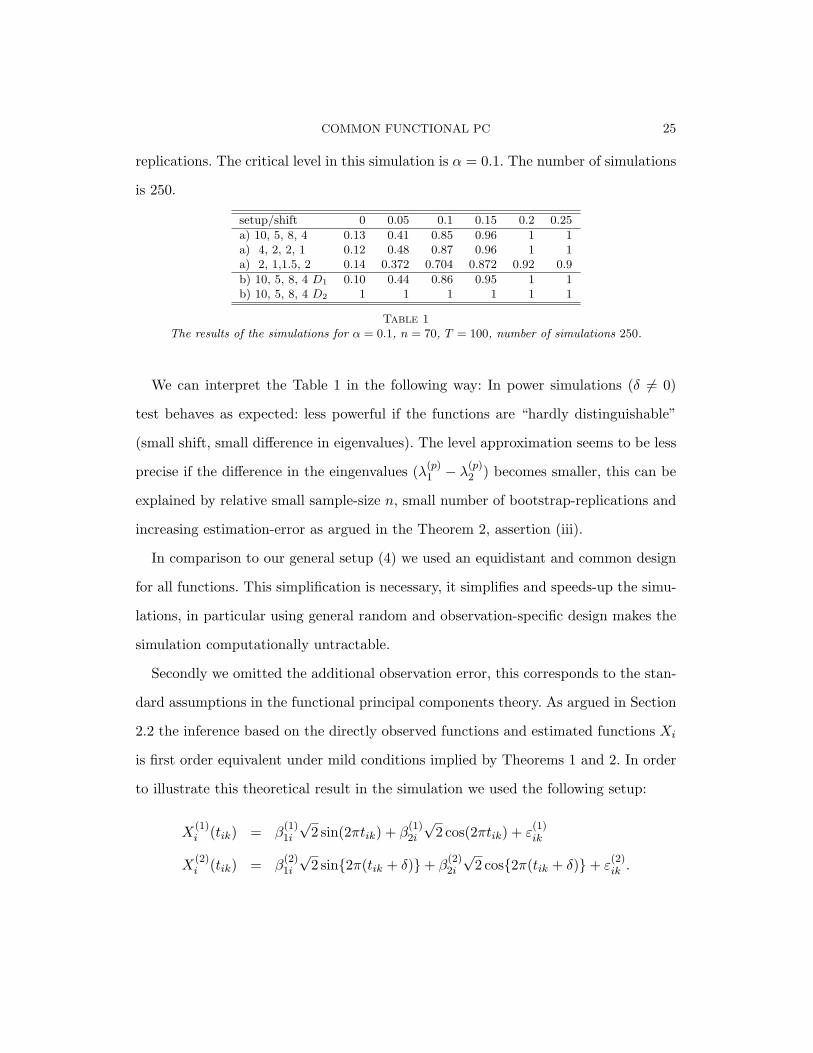
setup/shift 0 0.05 0.1 0.15 0.2 0.25
a) 10, 5, 8, 4 0.13 0.41 0.85 0.96 1 1a) 4, 2, 2, 1 0.12 0.48 0.87 0.96 1 1a) 2, 1,1.5, 2 0.14 0.372 0.704 0.872 0.92 0.9
b) 10, 5, 8, 4 D1 0.10 0.44 0.86 0.95 1 1b) 10, 5, 8, 4 D2 1 1 1 1 1 1
Table 1The results of the simulations for α = 0.1, n = 70, T = 100, number of simulations 250.
We can interpret the Table 1 in the following way: In power simulations (δ 6= 0)
test behaves as expected: less powerful if the functions are “hardly distinguishable”
(small shift, small difference in eigenvalues). The level approximation seems to be less
precise if the difference in the eingenvalues (λ(p)1 − λ
(p)2 ) becomes smaller, this can be
explained by relative small sample-size n, small number of bootstrap-replications and
increasing estimation-error as argued in the Theorem 2, assertion (iii).
In comparison to our general setup (4) we used an equidistant and common design
for all functions. This simplification is necessary, it simplifies and speeds-up the simu-
lations, in particular using general random and observation-specific design makes the
simulation computationally untractable.
Secondly we omitted the additional observation error, this corresponds to the stan-
dard assumptions in the functional principal components theory. As argued in Section
2.2 the inference based on the directly observed functions and estimated functions Xi
is first order equivalent under mild conditions implied by Theorems 1 and 2. In order
to illustrate this theoretical result in the simulation we used the following setup:
X(1)i (tik) = β
(1)1i
√2 sin(2πtik) + β
(1)2i
√2 cos(2πtik) + ε
(1)ik
X(2)i (tik) = β
(2)1i
√2 sin2π(tik + δ)+ β
(2)2i
√2 cos2π(tik + δ)+ ε
(2)ik .
26 M. BENKO, W. HARDLE AND A.KNEIP
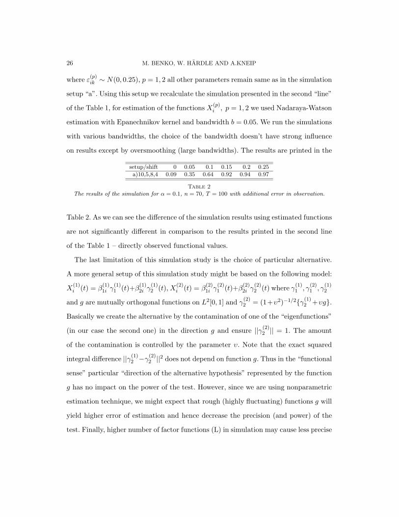
where ε(p)ik ∼ N(0, 0.25), p = 1, 2 all other parameters remain same as in the simulation
setup “a”. Using this setup we recalculate the simulation presented in the second “line”
of the Table 1, for estimation of the functions X(p)i , p = 1, 2 we used Nadaraya-Watson
estimation with Epanechnikov kernel and bandwidth b = 0.05. We run the simulations
with various bandwidths, the choice of the bandwidth doesn’t have strong influence
on results except by oversmoothing (large bandwidths). The results are printed in the
setup/shift 0 0.05 0.1 0.15 0.2 0.25
a)10,5,8,4 0.09 0.35 0.64 0.92 0.94 0.97
Table 2The results of the simulation for α = 0.1, n = 70, T = 100 with additional error in observation.
Table 2. As we can see the difference of the simulation results using estimated functions
are not significantly different in comparison to the results printed in the second line
of the Table 1 – directly observed functional values.
The last limitation of this simulation study is the choice of particular alternative.
A more general setup of this simulation study might be based on the following model:
X(1)i (t) = β
(1)1i γ
(1)1 (t)+β
(1)2i γ
(1)2 (t), X
(2)i (t) = β
(2)1i γ
(2)1 (t)+β
(2)2i γ
(2)2 (t) where γ
(1)1 , γ
(2)1 , γ
(1)2
and g are mutually orthogonal functions on L2[0, 1] and γ(2)2 = (1+υ2)−1/2γ(1)
2 +υg.Basically we create the alternative by the contamination of one of the “eigenfunctions”
(in our case the second one) in the direction g and ensure ||γ(2)2 || = 1. The amount
of the contamination is controlled by the parameter υ. Note that the exact squared
integral difference ||γ(1)2 −γ
(2)2 ||2 does not depend on function g. Thus in the “functional
sense” particular “direction of the alternative hypothesis” represented by the function
g has no impact on the power of the test. However, since we are using nonparametric
estimation technique, we might expect that rough (highly fluctuating) functions g will
yield higher error of estimation and hence decrease the precision (and power) of the
test. Finally, higher number of factor functions (L) in simulation may cause less precise
COMMON FUNCTIONAL PC 27
approximation of critical values and more bootstrap replications and larger sample-
size may be needed. This can also be expected from the Theorem 2 in Section 2.2 – the
variance of the estimated eigenfunctions depends on all eigenfunctions corresponding
to non-zero eingenvalues.
4. Implied Volatility Analysis. In this section we present an application of
the method discussed in previous sections to the implied volatilities of European op-
tions on the German stock index (ODAX). Implied volatilities are derived from the
Black-Scholes (BS) pricing formula for European options, see Black & Scholes (1973).
European call and put options are derivatives written on an underlying asset with
price process Si, which yield the pay-off max(SI −K, 0) and max(K − SI , 0). Here i
denotes the current day, I the expiration day and K the strike price. Time to maturity
is defined as τ = I − i. The BS pricing formula for a Call option is:
Ci(Si,K, τ, r, σ) = SiΦ(d1)−Ke−rτΦ(d2) (15)
where d1 = ln(Si/K)+(r+σ2/2)τσ√
τ, d2 = d1 − σ
√τ , r is the riskless interest rate, σ is the
(unknown and constant) volatility parameter, and Φ denotes the c.d.f. of a normal
distributed variable. In (15) we assume the zero-dividend case. The Put option price
Pi can be obtained from the put-call parity Pi = Ci − Si + e−τrK.
The implied volatility σ is defined as the volatility σ, for which the BS price Ci in
(15) equals the price Ci observed on the market. For a single asset, we obtain at each
time point (day i) and for each maturity τ a IV function στi (K). Practitioners often
rescale the strike dimension by plotting this surface in terms of (futures) moneyness
κ = K/Fi(τ), where Fi(τ) = Sierτ .
Clearly, for given parameters Si, r,K, τ the mapping from prices to IVs is a one-to-
one mapping. In the financial practice the IV is often used for quoting the European

28 M. BENKO, W. HARDLE AND A.KNEIP
options since it reflects the “uncertainity” of the financial market better than the
option prices. It is also known that if the stock price drops, the IV raises (so called
leverage effect) that motivates hedging strategies based on IVs. Consequently, for the
purpose of this application we will regard the BS-IV as an individual financial variable.
The practical relevance of such approach is justified by the volatility based financial
products such as VDAX, that are commonly traded on the option markets.
The goal of this analysis is to study the dynamics of the IV functions for different
maturities. More specifically, our aim is to construct low dimensional factor models
based on the truncated Karhunen-Loeve expansions (1) for the log-returns of the
IV functions of options with different maturities and compare these factor models
using the methodology presented in the previous sections. Analysis of IVs based on a
low-dimensional factor model gives directly a descriptive insight into the structure of
distribution of the log-IV-returns – structure of the factors and empirical distribution
of the factor loadings may be a good starting point for further pricing models. In
practice such a factor model can also be used in Monte-Carlo based pricing methods
and for risk-management (hedging) purposes. For comprehensive monographs on IV
and IV-factor models, see Hafner (2004) or Fengler (2005b).
The idea of constructing and analyzing the factor models for log-IV-returns for
different maturities was originally proposed by Fengler, Hardle & Villa (2003), who
studied the dynamics of the IV via PCA on discretized IV functions for different
maturity groups and tested the Common Principal Components (CPC) hypotheses
(equality of eigenvectors and eigenspaces for different groups). Fengler, Hardle & Villa
(2003) proposed a PCA-based factor models for log-IV-returns on (short) maturi-
ties 1,2 and 3 months and grid of moneyness [0.85, 0.9, 0.95, 1, 1.05, 1.1]. They showed
that the factor functions do not significantly differ and only the factor loadings differ
COMMON FUNCTIONAL PC 29
across maturity groups. Their method relies on the CPC methodology introduced by
Flury (1988) which is based on maximum likelihood estimation under the assumption
of multivariate normality. The log-IV-returns are extracted by the two-dimensional
Nadaraya-Watson estimate.
The main aim of this application is to verify their results in a functional sense.
Doing so, we overcome two basic weaknesses of their approach. Firstly, the factor
model proposed by Fengler, Hardle & Villa (2003) is performed only on a sparse
design of moneyness. However, in practice (e.g. in Monte-Carlo pricing methods) eval-
uation of the model on a fine grid is needed. Using the functional PCA approach we
may overcome this difficulty and evaluate the factor model on an arbitrary fine grid.
The second difficulty of the procedure proposed by Fengler, Hardle & Villa (2003)
stems from the data design – on the exchange we cannot observe options with desired
maturity on each day and we need to estimate them from the IV-functions with ma-
turities observed on the particular day. Consequently, the two-dimensional Nadaraya-
Watson estimator proposed by Fengler, Hardle & Villa (2003) results essentially in the
(weighted) average of the IVs (with closest maturities) observed on a particular day,
which may affect the test of the common eigenfunction hypothesis. We use the linear
interpolation scheme in the total variance σ2TOT,i(κ, τ) def= (στ
i (κ))2τ, in order to recover
the IV functions with fixed maturity (on day i). This interpolation scheme is based
on the arbitrage arguments originally proposed by Kahale (2004) for zero-dividend
and zero-interest rate case and generalized for deterministic interest rate by Fengler
(2005). More precisely, having IVs with maturities observed on a particular day i:
στjii (κ), ji = 1, . . . , pτi , we calculate the corresponding total variance σTOT,i(κ, τji).
From these total variances we linearly interpolate the total variance with the desired
maturity from the nearest maturities observed on day i. The total variance can be

30 M. BENKO, W. HARDLE AND A.KNEIP
easily transformed to corresponding IV στi (κ). As the last step we calculate the log-
returns4 log στi (κ) def= log στ
i+1(κ)−log στi (κ). The log-IV-returns are observed for each
maturity τ on a discrete grid κτik. We assume that observed log-IV-return4 log στ
i (κτik)
consists of true log-return of the IV function denoted by 4 log στi (κτ
ik) and possibly of
some additional error ετik. By setting Y τ
ik := 4 log στi (κτ
ik), Xτi (κ) := 4 log στ
i (κ) we
obtain an analogue of the model (4) with the argument κ:
Y τik = Xτ
i (κik) + ετik, i = 1, . . . , nτ . (16)
In order to simplify the notation and make the connection with the theoretical part
clear we will use the notation of (16).
For our analysis we use a recent data set containing daily data from January 2004 to
June 2004 from the German-Swiss exchange (EUREX). Violations of the arbitrage-free
assumptions (“obvious” errors in data) were corrected using the procedure proposed
by Fengler (2005). Similarly to Fengler, Hardle & Villa (2003) we excluded options
with maturity smaller then 10 days, since these option-prices are known to be very
noisy, partially because of a special and arbitrary setup in the pricing systems of
the dealers. Using the interpolation scheme described above we calculate the log-IV-
returns for two maturity groups: “1M” group with maturity τ = 0.12 (measured in
years) and “3M” group with maturity τ = 0.36. The observed log-IV-returns are
denoted by Y 1Mik , k = 1, . . . ,K1M
i , Y 3Mik , k = 1, . . . ,K3M
i . Since we ensured that for
no i, the interpolation procedure uses data with the same maturity for both groups,
this procedure has no impact on the independence of both samples.
COMMON FUNCTIONAL PC 31
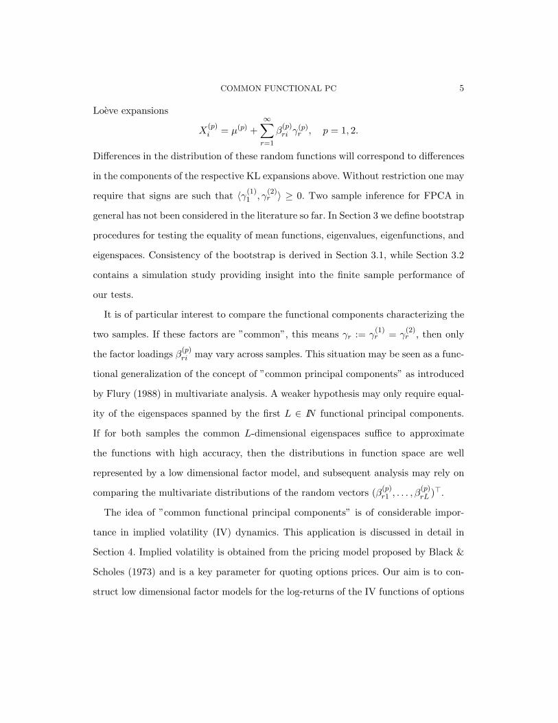
log IV returns, 1M
-0.15
-0.10
-0.05
0.00
0.05
0.10
0.15
0.85 0.90 0.95 ATM 1.05
-0.15
-0.10
-0.05
0.00
0.05
0.10
0.15
0.85 0.90 0.95 ATM 1.05
log IV returns, 3M
-0.15
-0.10
-0.05
0.00
0.05
0.10
0.15
0.85 0.90 0.95 ATM 1.05
-0.15
-0.10
-0.05
0.00
0.05
0.10
0.15
0.85 0.90 0.95 ATM 1.05
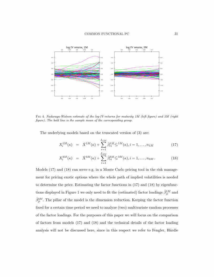
Fig 4. Nadaraya-Watson estimate of the log-IV-returns for maturity 1M (left figure) and 3M (rightfigure). The bold line is the sample mean of the corresponding group.
The underlying models based on the truncated version of (3) are:
X1Mi (κ) = X1M (κ) +
L1M∑
r=1
β1Mri γr
1M (κ), i = 1, . . . , n1M (17)
X3Mi (κ) = X3M (κ) +
L3M∑
r=1
β3Mri γr
3M (κ), i = 1, . . . , n3M . (18)
Models (17) and (18) can serve e.g. in a Monte Carlo pricing tool in the risk manage-
ment for pricing exotic options where the whole path of implied volatilities is needed
to determine the price. Estimating the factor functions in (17) and (18) by eigenfunc-
tions displayed in Figure 1 we only need to fit the (estimated) factor loadings β1Mji and
β3Mji . The pillar of the model is the dimension reduction. Keeping the factor function
fixed for a certain time period we need to analyze (two) multivariate random processes
of the factor loadings. For the purposes of this paper we will focus on the comparison
of factors from models (17) and (18) and the technical details of the factor loading
analysis will not be discussed here, since in this respect we refer to Fengler, Hardle

32 M. BENKO, W. HARDLE AND A.KNEIP
& Villa (2003), who proposed to fit the factor loadings by centered normal distribu-
tions with diagonal variance matrix containing the corresponding eigenvalues. For a
deeper discussion of the fitting of factor loadings using a more sophisticated approach,
basically based on (possibly multivariate) GARCH models, see Fengler (2005b).
From our data set we obtained 88 functional observations for the 1M group (n1M )
and 125 observations for the 3M group (n3M ). We will estimate the model on the
interval for futures moneyness κ ∈ [0.8, 1.1]. In comparison to Fengler, Hardle & Villa
(2003) we may estimate models (17) and (18) on an arbitrary fine grid (we used an
equidistant grid of 500 points on the interval [0.8, 1.1]). For illustration, the Nadaraya-
Watson (NW) estimator of resulting log-returns is plotted in Figure 4. The smoothing
parameters have been chosen in accordance with the requirements in Section 2.2. As
argued in Section 2.2, we should use small smoothing parameters in order to avoid
a possible bias in the estimated eigenfunctions. Thus we use for each i essentially
the smallest bandwidth bi that guarantees that estimator Xi is defined on the entire
support [0.8, 1.1].
Using the procedures described in Section 2.1 we first estimate the eigenfunctions of
both maturity groups. The estimated eigenfunctions are plotted in Figure 1. The struc-
ture of the eigenfunctions is in accordance with other empirical studies on IV-surfaces.
For a deeper discussion and economical interpretation see for example Fengler, Hardle
& Mammen (2005) or Fengler, Hardle & Villa (2003).
Clearly, the ratio of the variance explained by the kth factor function is given by
the quantity ν1Mk = λ1M
k /∑n1M
j=1 λ1Mj for the 1M group and, correspondingly, by ν3M
k
for the 3M group. In Table 3 we list the contributions of the factor functions. Looking
at Table 3 we can see that 4th factor functions explain less than 1% of the variation.
This number was the “threshold” for the choice of L1M and L2M .
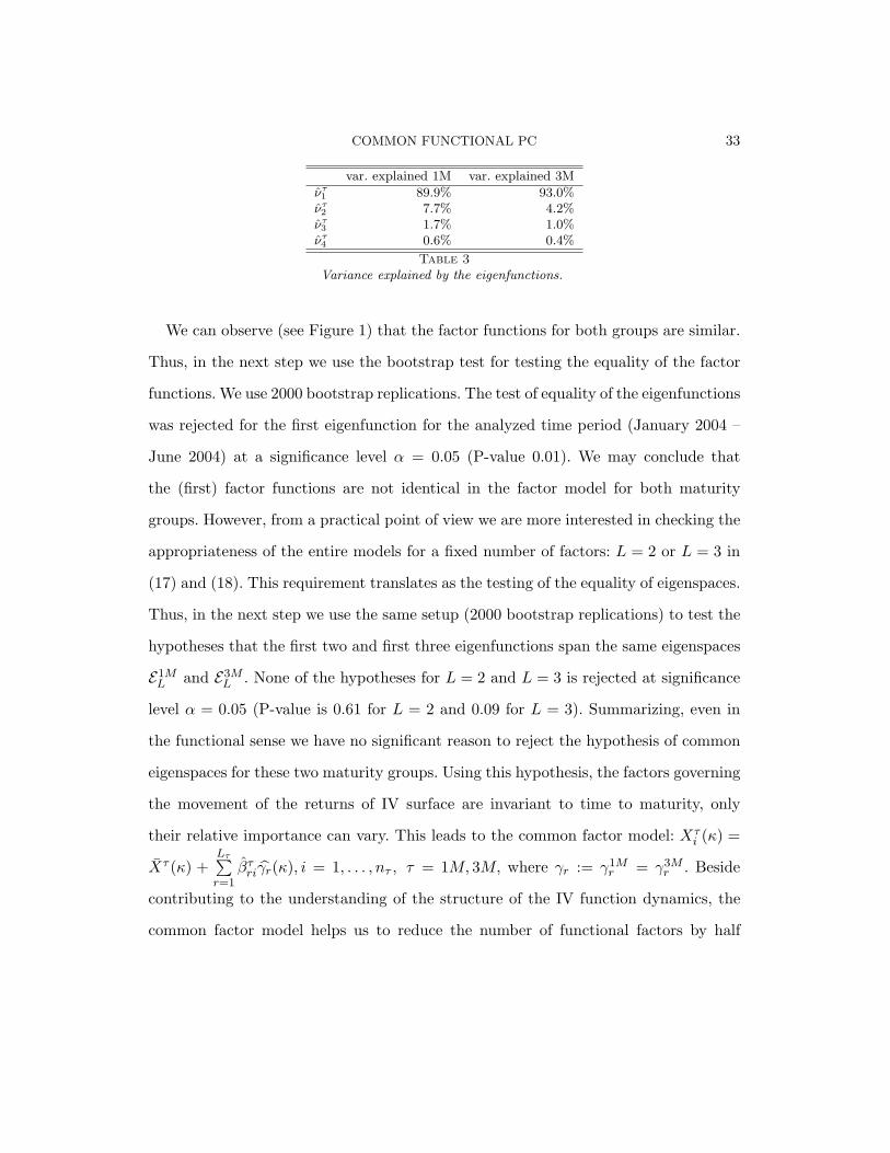
COMMON FUNCTIONAL PC 33
var. explained 1M var. explained 3M
ντ1 89.9% 93.0%
ντ2 7.7% 4.2%
ντ3 1.7% 1.0%
ντ4 0.6% 0.4%
Table 3Variance explained by the eigenfunctions.
We can observe (see Figure 1) that the factor functions for both groups are similar.
Thus, in the next step we use the bootstrap test for testing the equality of the factor
functions. We use 2000 bootstrap replications. The test of equality of the eigenfunctions
was rejected for the first eigenfunction for the analyzed time period (January 2004 –
June 2004) at a significance level α = 0.05 (P-value 0.01). We may conclude that
the (first) factor functions are not identical in the factor model for both maturity
groups. However, from a practical point of view we are more interested in checking the
appropriateness of the entire models for a fixed number of factors: L = 2 or L = 3 in
(17) and (18). This requirement translates as the testing of the equality of eigenspaces.
Thus, in the next step we use the same setup (2000 bootstrap replications) to test the
hypotheses that the first two and first three eigenfunctions span the same eigenspaces
E1ML and E3M
L . None of the hypotheses for L = 2 and L = 3 is rejected at significance
level α = 0.05 (P-value is 0.61 for L = 2 and 0.09 for L = 3). Summarizing, even in
the functional sense we have no significant reason to reject the hypothesis of common
eigenspaces for these two maturity groups. Using this hypothesis, the factors governing
the movement of the returns of IV surface are invariant to time to maturity, only
their relative importance can vary. This leads to the common factor model: Xτi (κ) =
Xτ (κ) +Lτ∑r=1
βτriγr(κ), i = 1, . . . , nτ , τ = 1M, 3M, where γr := γ1M
r = γ3Mr . Beside
contributing to the understanding of the structure of the IV function dynamics, the
common factor model helps us to reduce the number of functional factors by half

34 M. BENKO, W. HARDLE AND A.KNEIP
compared to models (17) and (18). Furthermore, from the technical point of view,
we also obtain an additional dimension reduction and higher estimation precision,
since under this hypothesis we may estimate the eigenfunctions from the (individually
centered) pooled sample Xi(κ)1M , i = 1, . . . , n1M , X3Mi (κ), i = 1, . . . , n3M . The main
improvement compared to the multivariate study by Fengler, Hardle & Villa (2003)
is that our test is performed in the functional sense – it doesn’t depend on particular
discretization and our factor model can be evaluated on an arbitrary fine grid.
COMMON FUNCTIONAL PC 35
5. Appendix: Mathematical Proofs. In the following, ‖v‖ = (∫ 10 v(t)2dt)1/2
will denote the L2-norm for any square integrable function v. At the same time, ‖a‖ =
( 1k
∑ki=1 a2
i )1/2 will indicate the Euclidean norm, whenever a ∈ Rk is a k-vector for
some k ∈ IN .
In the proof of Theorem 1, Eε and Varε denote expectation and variance with re-
spect to ε only (i.e. conditional on tij and Xi).
Proof of Theorem 1.
Recall the definition of the χi(t) and note that χi(t) = χXi (t) + χε
i (t), where
χεi (t) =
Ti∑
j=1
εi(j)I
(t ∈
[ti(j−1) + ti(j)
2,ti(j) + ti(j+1)
2
])
as well as
χXi (t) =
Ti∑
j=1
Xi(ti(j))I(
t ∈[ti(j−1) + ti(j)
2,ti(j) + ti(j+1)
2
])
for t ∈ [0, 1], ti(0) = −ti(1) and ti(Ti+1) = 2− ti(Ti). Similarly, χ∗i (t) = χX∗i (t) + χε∗
i (t).
By Assumption 2, E(|ti(j) − ti(j−1)|s
)= O(T−s) for s = 1, . . . , 4, and the conver-
gence is uniform in j < n. Our assumptions on the structure of Xi together with some
straightforward Taylor expansions then lead to
〈χi, χj〉 = 〈Xi, Xj〉+Op(1/T )
and
〈χi, χ∗i 〉 = ‖Xi‖2 +Op(1/T ).
36 M. BENKO, W. HARDLE AND A.KNEIP
Moreover,
Eε(〈χεi , χ
Xj 〉) = 0, Eε(‖χε
i‖2) = σ2i ,
Eε(〈χεi , χ
ε∗i 〉) = 0, Eε(〈χε
i , χε∗i 〉2) = Op(1/T ),
Eε(〈χεi , χ
Xj 〉2) = Op(1/T ), Eε(〈χε
i , χXj 〉〈χε
k, χXl 〉) = 0 for i 6= k,
Eε(〈χεi , χ
εj〉〈χε
i , χεk〉) = 0 for j 6= k and Eε(‖χε
i‖4) = Op(1)
hold (uniformly) for all i, j = 1, . . . , n.
Consequently, Eε(‖χ‖2 − ‖X‖2) = Op(T−1 + n−1).
When using these relations, it is easily seen that for all i, j = 1, . . . , n
Mij −Mij = Op(T−1/2 + n−1) and tr(M −M)21/2 = Op(1 + nT−1/2). (19)
Since the orthonormal eigenvectors pq of M satisfy ‖pq‖ = 1, we furthermore obtain
for any i = 1, . . . , n and all q = 1, 2, . . .
n∑
j=1
pjq
Mij −Mij −
∫ 1
0χε
i (t)χXj (t)dt
= Op(T−1/2 + n−1/2) (20)
as well asn∑
j=1
pjq
∫ 1
0χε
i (t)χXj (t)dt = Op
(n1/2
T 1/2
)(21)
andn∑
i=1
ai
n∑
j=1
pjq
∫ 1
0χε
i (t)χXj (t)dt = Op
(n1/2
T 1/2
)(22)
for any further vector a with ‖a‖ = 1.
Recall that the j-th largest eigenvalue lj satisfies nλj = lj . Since by assumption
infs6=r |λr − λs| > 0, the results of Dauxois, Pousse & Romain (1982) imply that λr
converges to λr as n →∞, and sups6=r1
|λr−λs| = Op(1), which leads to sups 6=r1
|lr−ls| =
Op(1/n). Assertion a) of Lemma A of Kneip & Utikal (2001) together with (19) - (22)
then implies that
COMMON FUNCTIONAL PC 37
∣∣∣∣∣λr − lrn
∣∣∣∣∣ = n−1|lr − lr| = n−1|p>r (M −M)pr|+Op(T−1 + n−1)
= Op(nT )−1/2 + T−1 + n−1. (23)
When analyzing the difference between the estimated and true eigenvectors pr and
pr, assertion b) of Lemma A of Kneip & Utikal (2001) together with (19) lead to
pr − pr = −Sr(M −M)pr +Rr, with ‖Rr‖ = Op(T−1 + n−1) (24)
and Sr =∑
s6=r1
ls−lrpsp
>s . Since sup‖a‖=1 a>Sra ≤ sups6=r
1|lr−ls| = Op(1/n), we can
conclude that
‖pr − pr‖ = Op(T−1/2 + n−1), (25)
and our assertion on the sequence n−1∑
i(βri − βri;T )2 is an immediate consequence.
Let us now consider assertion ii). The well-known properties of local linear estima-
tors imply that |EεXi(t)−Xi(t)| = Op(b2) as well as VarεXi(t) = Op(Tb), and
the convergence is uniform for all i, n. Furthermore, due to the independence of the
error term εij , CovεXi(t), Xj(t) = 0 for i 6= j. Therefore,
|γr(t)− 1√lr
n∑
i=1
pirXi(t)| = Op(b2 +1√nTb
).
On the other hand, (19) - (25) imply that with X(t) = (X1(t), . . . , Xn(t))>
|γr;T (t)− 1√lr
n∑
i=1
pirXi(t)|
= | 1√lr
n∑
i=1
(pir − pir)Xi(t) +1√lr
n∑
i=1
(pir − pir)Xi(t)−Xi(t)|+Op(T−1 + n−1)
=‖SrX(t)‖√
lr|p>r (M −M)Sr
X(t)‖SrX(t)‖|+Op(b2T−1/2 + T−1b−1/2 + n−1)
= Op(n−1/2T−1/2 + b2T−1/2 + T−1b−1/2 + n−1).
This proves the theorem.
38 M. BENKO, W. HARDLE AND A.KNEIP
Proof of Theorem 2:
First consider assertion i). By definition,
X(t)− µ(t) = n−1n∑
i=1
Xi(t)− µ(t) =∑
r
(n−1n∑
i=1
βri)γr(t).
Recall that, by assumption, βri are independent, zero mean random variables with
variance λr, and that the above series converges with probability 1. When defining the
truncated series
V (q) =q∑
r=1
(n−1n∑
i=1
βri)γr(t),
standard central limit theorems therefore imply that√
nV (q) is asymptotically
N(0,∑q
r=1 λrγr(t)2) distributed for any possible q ∈ IN .
The assertion of a N(0,∑∞
r=1 λrγr(t)2) limiting distribution now is a consequence
of the fact that for all δ1, δ2 > 0 there exists a qδ such that
P|√nV (q)−√n∑
r(n−1
∑ni=1 βri)γr(t)| > δ1 < δ2 for all q ≥ qδ and all n sufficiently
large.
In order to prove assertions i) and ii), consider some fixed r ∈ 1, 2, . . . with λr−1 >
λr > λr+1. Note that Γ as well as Γn are nuclear, self-adjoint and non-negative linear
operators with Γv =∫
σ(t, s)v(s)ds and Γnv =∫
σ(t, s)v(s)ds, v ∈ L2[0, 1]. For m ∈ IN
let Πm denote the orthogonal projector from L2[0, 1] into the m-dimensional linear
space spanned by γ1, . . . , γm, i.e. Πmv =∑m
j=1〈v, γj〉γj , v ∈ L2[0, 1]. Now consider
the operator ΠmΓnΠm as well as its eigenvalues and corresponding eigenfunctions
denoted by λ1,m ≥ λ2,m ≥ . . . and γ1,m, γ2,m, . . . , respectively. It follows from well-
known results in Hilbert space theory that ΠmΓnΠm converges strongly to Γn as
m →∞ . Furthermore, we obtain (Rayleigh-Ritz theorem)
limm→∞ λr,m = λr, and lim
m→∞ ‖γr − γr,m‖ = 0 if λr−1 > λr > λr+1. (26)
COMMON FUNCTIONAL PC 39
Note that under the above condition γr is uniquely determined up to sign, and recall
that we always assume that the right “versions” (with respect to sign) are used so that
〈γr, γr,m〉 ≥ 0. By definition βji =∫
γj(t)Xi(t)−µ(t)dt, and therefore∫
γj(t)Xi(t)−X(t)dt = βji− βj as well as Xi− X =
∑j(βji− βj)γj , where βj = 1
n
∑ni=1 βji. When
analyzing the structure of ΠmΓnΠm more deeply, we can verify that ΠmΓnΠmv =∫
σm(t, s)v(s)ds, v ∈ L2[0, 1], with
σm(t, s) = gm(t)>Σmgm(s),
where gm(t) = (γ1(t), . . . , γm(t))>, and where Σm is the m × m matrix with ele-
ments 1n
∑ni=1(βji − βj)(βki − βk)j,k=1,...,m. Let λ1(Σm) ≥ λ2(Σm) ≥ · · · ≥ λm(Σm)
and ζ1,m, . . . , ζm,m denote eigenvalues and corresponding eigenvectors of Σm. Some
straightforward algebra then shows that
λr,m = λr(Σm), γr,m = gm(t)>ζr,m. (27)
We will use Σm to represent the m×m diagonal matrix with diagonal entries λ1 ≥ · · · ≥λm. Obviously, the corresponding eigenvectors are given by the m-dimensional unit
vectors denoted by e1,m, . . . , em,m. Lemma A of Kneip & Utikal (2001) now implies that
the differences between eigenvalues and eigenvectors of Σm and Σm can be bounded
by
λr,m−λr = trer,me>r,m(Σm−Σm)+Rr,m, with Rr,m ≤ 6 sup‖a‖=1 a>(Σm − Σm)2amins |λs − λr| ,
(28)
ζr,m−er,m = −Sr,m(Σm−Σm)er,m+R∗r,m, with ‖R∗
r,m‖ ≤6 sup‖a‖=1 a>(Σm − Σm)2a
mins |λs − λr|2 ,
(29)
where Sr,m =∑
s 6=r1
λs−λres,me>s,m.

40 M. BENKO, W. HARDLE AND A.KNEIP
Assumption 1 implies E(βr) = 0, Var(βr) = λrn , and with δii = 1 as well as δij = 0
for i 6= j we obtain
E sup‖a‖=1
a>(Σm − Σm)2a ≤ Etr[(Σm − Σm)2] = Em∑
j,k=1
[1n
n∑
i=1
(βji − βj)(βki − βk)− δjkλj ]2
≤ E∞∑
j,k=1
[1n
n∑
i=1
(βji − βj)(βki − βk)− δjkλj ]2 =1n
(∑
j
∑
k
Eβ2jiβ
2ki) + O(n−1) = O(n−1)
(30)
for all m. Since trer,me>r,m(Σm − Σm) = 1n
∑ni=1(βri − βr)2 − λr, (26), (27), (28),
and (30) together with standard central limit theorems imply that
√n(λr − λr) =
1√n
n∑
i=1
(βri − βr)2 − λr +Op(n−1/2)
=1√n
n∑
i=1
[(βri)2 − E(βri)2
]+Op(n−1/2) L→ N(0, Λr). (31)
It remains to prove assertion iii). Relations (27) and (29) lead to
γr,m(t)− γr(t) = gm(t)>(ζr,m − er,m)
= −m∑
s 6=r
1
n(λs − λr)
n∑
i=1
(βsi − βs)(βri − βr)
γs(t) + gm(t)>R∗
r,m, (32)
where due to (30) the function gm(t)>R∗r,m satisfies
E(‖g>mR∗r,m‖) = E(‖R∗
r,m‖) ≤6
n mins |λs − λr|2
∑
j
∑
k
Eβ2
jiβ2ki
+ O
(n−1
)
for all m. By Assumption 1 the series in (32) converge with probability 1 as m →∞.
Obviously, the event λr−1 > λr > λr+1 occurs with probability 1. Since m is arbi-
trary, we can therefore conclude from (26) and (32) that
γr(t)− γr(t) = −∑
s 6=r
1
n(λs − λr)
n∑
i=1
(βsi − βs)(βri − βr)
γs(t) + R∗
r(t) (33)
= −∑
s 6=r
1
n(λs − λr)
n∑
i=1
βsiβri
γs(t) + Rr(t),
COMMON FUNCTIONAL PC 41
where ‖R∗r‖ = Op(n−1) as well as ‖Rr‖ = Op(n−1). Moreover,
√n
∑s 6=r
1
n(λs−λr)
∑ni=1 βsiβri
γs(t) is a zero mean random variable with variance
∑q 6=r
∑s6=r
E[β2riβqiβsi]
(λq−λr)(λs−λr)γq(t)γs(t) < ∞. By Assumption 1 it follows from standard
central limit arguments that for any q ∈ IN the truncated series√
nW (q) def=√
n∑q
s=1,s 6=r[1
n(λs−λr)
∑ni=1 βsiβri]γs(t) is asymptotically normal distributed.
The asserted asymptotic normality of the complete series then follows from an argu-
ment similar to the one used in the proof of Assertion i).
Proof of Theorem 3: The results of Theorem 2 imply that
n∆1 =∫ (∑
r
1√q1n1
n1∑
i=1
β(1)ri γ(1)
r (t)−∑
r
1√q2n2
n2∑
i=1
β(2)ri γ(2)
r (t)
)2
dt. (34)
Furthermore, independence of X(1)i and X
(2)i together with (31) imply that
√n[λ(1)
r − λ(1)r − λ(2)
r − λ(2)r ] L→ N
(0,
Λ(1)r
q1+
Λ(2)r
q2
), and
n
Λ(1)rq1
+ Λ(2)rq2
∆3,rL→ χ2
1.
(35)
Furthermore, (33) leads to
n∆2,r =
∥∥∥∥∥∥∑
s 6=r
1
√q1n1(λ
(1)s − λ
(1)r )
n1∑
i=1
β(1)si β
(1)ri
γ(1)
s
−∑
s6=r
1
√q2n2(λ
(2)s − λ
(2)r )
n2∑
i=1
β(2)si β
(2)ri
γ(2)
s
∥∥∥∥∥∥
2
+Op(n−1/2) (36)
42 M. BENKO, W. HARDLE AND A.KNEIP
and
n∆4,L = n
∫ ∫ [L∑
r=1
γ(1)r (t)γ(1)
r (u)− γ(1)r (u)+ γ(1)
r (u)γ(1)r (t)− γ(1)
r (t)
−L∑
r=1
γ(2)r (t)γ(2)
r (u)− γ(2)r (u)+ γ(2)
r (u)γ(2)r (t)− γ(2)
r (t)]2
dtdu +Op(n−1/2)
=∫ ∫ [
L∑r=1
∑
s>L
1√
q1n1(λ(1)s − λ
(1)r )
n1∑
i=1
β(1)si β
(1)ri γ(1)
r (t)γ(1)s (u) + γ(1)
r (u)γ(1)s (t)
−L∑
r=1
∑
s>L
1√
q2n2(λ(2)s − λ
(2)r )
n2∑
i=1
β(2)si β
(2)ri γ(2)
r (t)γ(2)s (u) + γ(2)
r (u)γ(2)s (t)
]2
dtdu +Op(n−1/2)
(37)
In order to verify (37) note that∑L
r=1
∑Ls=1,s 6=r
1
(λ(p)s −λ
(p)r )
aras = 0 for p = 1, 2
and all possible sequences a1, . . . , aL. It is clear from our assumptions that all sums
involved converge with probability 1. Recall that E(β(p)ri β
(p)si ) = 0, p = 1, 2 for r 6= s.
It follows that X(p)r := 1√
qpnp
∑s 6=r
∑np
i=1β
(p)si β
(p)ri
λ(p)s −λ
(p)r
γ(p)s , p = 1, 2, is a continuous,
zero mean random function on L2[0, 1], and, by assumption, E(‖X(p)r ‖2) < ∞. By
Hilbert space central limit theorems (see, e.g, Araujo & Gine (1980)) X(p)r thus con-
verges in distribution to a Gaussian random function ξ(p)r as n → ∞. Obviously, ξ
(1)r
is independent of ξ(2)r . We can conclude that n∆4,L possesses a continuous limit dis-
tribution F4,L defined by the distribution of∫ ∫ [
L∑r=1ξ(1)
r (t)γ(1)r (u) + ξ
(1)r (u)γ(1)
r (t)
−∑Lr=1ξ(2)
r (t)γ(2)r (u) + ξ
(2)r (u)γ(2)
r (t)]2
dtdu. Similar arguments show the existence
of continuous limit distributions F1 and F2,r of n∆1 and n∆2,r.
For given q ∈ IN define vectors b(p)i1 = (β(p)
1i , . . . , β(p)qi , )> ∈ Rq,
b(p)i2 = (β(p)
1i β(p)ri , . . . , β
(p)r−1,iβ
(p)ri , β
(p)r+1,iβ
(p)ri , . . . , β
(p)qi β
(p)ri )> ∈ Rq−1, and bi3 = (β(p)
1i β(p)2i ,
. . . , β(p)qi β
(p)Li )> ∈ R(q−1)L. When the infinite sums over r in (34) respectively s 6= r in
(36) and (37) are restricted to q ∈ IN components (i.e.∑
r and∑
s>L are replaced
by∑
r≤q and∑
L<s≤q), then the above relations can generally be presented as limits
COMMON FUNCTIONAL PC 43
n∆ = limq→∞n∆(q) of quadratic forms
n∆1(q) =
1√n1
∑n1i=1 b
(1)i1
1√n2
∑n2i=1 b
(2)i1
>
Qq1
1√n1
∑n1i=1 b
(1)i1
1√n2
∑n2i=1 b
(2)i1
,
n∆2,r(q) =
1√n1
∑n1i=1 b
(1)i2
1√n2
∑n2i=1 b
(2)i2
>
Qq2
1√n1
∑n1i=1 b
(1)i2
1√n2
∑n2i=1 b
(2)i2
,
n∆4,L(q) =
1√n1
∑n1i=1 b
(1)i3
1√n2
∑n2i=1 b
(2)i3
>
Qq3
1√n1
∑n1i=1 b
(1)i3
1√n2
∑n2i=1 b
(2)i3
, (38)
where the elements of the 2q×2q, 2(q−1)×2(q−1) and 2L(q−1)×2L(q−1) matrices
Qq1, Qq
2 and Qq3 can be computed from the respective (q-element) version of (34) - (37).
Assumption 1 implies that all series converge with probability 1 as q → ∞, and by
(34) - (37) it is easily seen that for all ε, δ > 0 there exist some q(ε, δ), n(ε, δ) ∈ IN
such that
P (|n∆1 − n∆1(q)| > ε) < δ, P (|n∆2,r − n∆2,r(q)| > ε) < δ,
P (|n∆4,L − n∆4,L(q)| > ε) < δ, (39)
hold for all q ≥ q(ε, δ) and all n ≥ n(ε, δ). For any given q, we have E(bi1) = E(bi2) =
E(bi3) = 0, and it follows from Assumption 1 that the respective covariance structures
can be represented by finite covariance matrices Ω1,q, Ω2,q, and Ω3,q. It therefore fol-
lows from our assumptions together with standard multivariate central limit theorems
that the vectors 1√n1
∑n1i=1(b
(1)ik )>, 1√
n2
∑n2i=1(b
(2)ik )>>, k = 1, 2, 3, are asymptotically
normal with zero means and covariance matrices Ω1,q, Ω2,q, and Ω3,q. One can thus
conclude that as n →∞
n∆1(q)L→ F1,q, n∆2,r(q)
L→ F2,r,q, n∆4,L(q) L→ F4,L,q, (40)
where F1,q, F2,r,q, F4,L,q denote the continuous distributions of the quadratic forms
z>1 Qq1z1, z>2 Qq
2z2, z>3 Qq3z3 with z1 ∼ N(0, Ω1,q), z2 ∼ N(0,Ω2,q), z3 ∼ N(0, Ω3,q). Since
44 M. BENKO, W. HARDLE AND A.KNEIP
ε, δ are arbitrary, (39) implies
limq→∞F1,q = F1, lim
q→∞F2,r,q = F2,r, limq→∞F4,L,q = F4,L. (41)
We now have to consider the asymptotic properties of bootstrapped eigenvalues
and eigenfunctions. Let X(p)∗ = 1np
∑np
i=1 X(p)∗i , β
(p)∗ri =
∫γ
(p)r (t)X(p)∗
i (t) − µ(t),β
(p)∗r = 1
np
∑np
i=1 β(p)∗ri , and note that
∫γ
(p)r (t)X(p)∗
i (t) − X(p)∗(t) = β(p)∗ri − β
(p)∗r .
When considering unconditional expectations, our assumptions imply that for p = 1, 2
E[β(p)∗ri ] = 0,E[(β(p)∗
ri )2] = λ(p)r , E[(β(p)∗
r )2] =λ
(p)r
np, E[(β(p)∗
ri )2 − λ(p)r ]2 = Λ(p)
r ,
E∞∑
l,k=1
[1np
np∑
i=1
(β(p)∗li − β
(p)∗l )(β(p)∗
ki − β(p)∗k )− δlkλ
(p)l ]2
=1np
(∑
l
Λ(p)l +
∑
l 6=k
λ(p)l λ
(p)k ) + O(n−1
p ). (42)
One can infer from(42) that the arguments used to prove Theorem 1 can be gener-
alized to approximate the difference between the bootstrap eigenvalues and eigenfunc-
tions λ(p)∗r , γ
(p)∗r and the true eigenvalues λ
(p)r , γ
(p)r . All infinite sums involved converge
with probability 1. Relation (31) then generalizes to
√np(λ(p)∗
r − λ(p)r ) =
√np(λ(p)∗
r − λ(p)r )−√np(λ(p)
r − λ(p)r )
=1√np
np∑
i=1
(β
(p)∗ri − β(p)∗
r
)2− 1√
np
np∑
i=1
(β
(p)ri − β(p)
r
)2+Op(n−1/2
p )
=1√np
np∑
i=1
(β(p)∗
ri )2 − 1np
np∑
k=1
(β(p)rk )2
+Op(n−1/2
p ). (43)
COMMON FUNCTIONAL PC 45
Similarly, (33) becomes
γ(p)∗r − γ(p)
r = γ(p)∗r − γ(p)
r − (γ(p)r − γ(p)
r )
= −∑
s 6=r
1
λ(p)s − λ
(p)r
1np
np∑
i=1
(β(p)∗si − β(p)∗
s )(β(p)∗ri − β(p)∗
r )
− 1
λ(p)s − λ
(p)r
1np
np∑
i=1
(β(p)si − β(p)
s )(β(p)ri − β(p)
r )
γ(p)
s (t) + R(p)∗r (t)
= −∑
s 6=r
1
λ(p)s − λ
(p)r
1np
np∑
i=1
(β
(p)∗si β
(p)∗ri − 1
np
np∑
k=1
β(p)sk β
(p)rk
)γ(p)
s (t) + R(p)∗r (t) (44)
where due to (29), (30), and (42) the remainder term satisfies ‖R(p)∗r ‖ = Op(n−1
p ).
We are now ready to analyze the bootstrap versions ∆∗ of the different ∆. First
consider ∆∗3,r and note that (β(p)∗
ri )2 are i.i.d. bootstrap resamples from (β(p)ri )2.
It therefore follows from basic bootstrap results that the conditional distribution of
1√np
∑np
i=1[(β(p)∗ri )2 − 1
np
∑np
k=1(β(p)rk )2] given Xp converges to the same N(0, Λ(p)
r ) limit
distribution as 1√np
∑np
i=1[(β(p)ri )2 − E(β(p)
ri )2]. Together with the independence of
(β(1)∗ri )2 and (β(2)∗
ri )2 the assertion of the theorem is an immediate consequence.
Let us turn to ∆∗1, ∆∗
2,r and ∆∗4,L. Using (42) - (44) it is then easily seen that
n∆∗1, n∆∗
2,r and n∆∗4,L admit expansions similar to (34), (36) and (37), when replacing
there 1√np
∑np
i=1 β(p)ri by 1√
np
∑np
i=1(β(p)∗ri − 1
np
∑np
k=1 β(p)rk ) as well as 1√
np
∑np
i=1 β(p)si β
(p)ri
by 1√np
∑np
i=1(β(p)∗si β
(p)∗ri − 1
np
∑np
k=1 β(p)sk β
(p)rk ).
Replacing β(p)ri , β
(p)si by β
(p)∗ri , β
(p)∗si leads to bootstrap analogs b
(p)∗ik of the vectors b
(p)ik ,
k = 1, 2, 3. For any q ∈ IN define bootstrap versions n∆∗1(q), n∆∗
3,r(q) and n∆∗4,L(q)
of n∆1(q), n∆3,r(q) and n∆∗4,L(q) by using
(1√n1
∑n1i=1(b
(1)∗ik − 1
n1
∑n1k=1 b
(1)ik )>, 1√
n2
∑n2i=1(b
(2)∗ik − 1
n2
∑n2k=1 b
(2)ik )>
)instead of
(1√n1
∑n1i=1(b
(1)ik )>, 1√
n2
∑n2i=1(b
(2)ik )>
), k = 1, 2, 3, in (38). Applying again (42) - (44)
46 M. BENKO, W. HARDLE AND A.KNEIP
one can conclude that for any ε > 0 there exists some q(ε) such that as n →∞
P (|n∆∗1 − n∆∗
1(q)| < ε) → 1,
P (|n∆∗2,r − n∆∗
2,r(q)| < ε) → 1,
P (|n∆∗4,L − n∆∗
4,L(q)| < ε) → 1, (45)
hold for all q ≥ q(ε). Of course, (45) generalizes to the conditional probabilities given
X1, X2.
In order to prove the theorem it thus only remains to show that for any given q and
all δ
|P (n∆(q) ≥ δ)− P (n∆∗(q) ≥ δ| X1,X2) | = Op(1) (46)
hold for either ∆(q) = ∆1(q) and ∆∗(q) = ∆∗1(q), ∆(q) = ∆2,r(q) and ∆∗(q) = ∆∗
2,r(q),
or ∆(q) = ∆4,L(q) and ∆∗(q) = ∆∗4,L(q). But note that for k = 1, 2, 3, E(bik) = 0,
b(j)∗ik are i.i.d. bootstrap resamples from b(p)
ik , and E(b(p)∗ik | X1,X2) = 1
np
∑np
k=1 b(p)ik
are the corresponding conditional means. It therefore follows from basic bootstrap re-
sults that as n →∞ the conditional distribution of(
1√n1
∑n1i=1(b
(1)∗ik − 1
n1
∑n1k=1 b
(1)ik )>, 1√
n2
∑n2i=1(b
(2)∗ik − 1
n2
∑n2k=1 b
(2)ik )>
)given X1, X2 con-
verges to the same N(0,Ωk,q)- limit distribution as(
1√n1
∑n1i=1(b
(1)ik )>, 1√
n2
∑n2i=1, (b
(2)ik )>
).
This obviously holds for all q ∈ IN , and (46) is an immediate consequence. The theorem
then follows from (39), (40), (41), (45) and (46).

COMMON FUNCTIONAL PC 47
REFERENCES
ARAUJO, A. & GINE, E. (1980). The Central Limit Theorem for Real and Banach Valued Random
Variables, Wiley, New York.
BESSE, P. & RAMSAY, J.(1986). Principal Components of Sampled Functions, Psychometrika, 51:
285-311.
BLACK, F. & SCHOLES, M. (1973). The Pricing of Options and Corporate Liabilities, Journal of
Political Economy, 81: 637-654.
DAUXOIS, J., POUSSE, A. & ROMAIN, Y. (1982). Asymptotic Theory for the Principal Component
Analysis of a Vector Random Function: Some Applications to Statistical Inference, Journal
of Multivariate Analysis 12: 136-154.
FAN, J. & HUANG, L. (1999). Nonparametric Estimation of Quadratic Regression Functionals,
Bernoulli 5: 927-949.
FENGLER, M. (2005). Arbitrage-free Smoothing of the Implied Volatility Surface SFB 649 Discussion
Paper No. 2005-019, SFB 649, Humboldt-Universitat zu Berlin.
FENGLER, M., HARDLE, W. & VILLA, P. (2003). The Dynamics of Implied Volatilities: A Common
Principle Components Approach, Review of Derivative Research 6: 179-202.
FENGLER, M., HARDLE, W. & MAMMEN, E. (2005). A Dynamic Semiparametric Factor Model
for Implied Volatility String Dynamics, SFB 649 Discussion Paper No. 2005-20, SFB 649
Humboldt-Univestitat zu Berlin.
FENGLER, M. (2005b). Semiparametric Modeling of Implied Volatility, Springer, Berlin.
FERRATY, F. & Vieu, P. (2006). Nonparametric Functional Data Analysis, Springer, New York.
FLURY, B. (1988). Common Principal Components and Related Models, Wiley, New York.
GIHMAN, I.I. & SKOROHOD, A.V. (1973). The Theory of Stochastic Processes II., Springer, New
York.
HALL, P. & Hosseini-Nasab, M. (2006). On Properties of Functional Principal Components Analysis,
Journal of the Royal Statistical Society, Series B, 68: 109-126.
HALL, P., MULLER, H.G. & WANG, J.L. (2006). Properties of Principal Components Methods for
Functional and Longitudial Data Analysis, Annals of Statistics 34: 1493-1517.
HALL, P., KAY, J.W. & TITTERINGTON, D.M. (1990). Asymptotically Optimal Difference-based
Estimation of Variance in Nonparametric Regression, Biometrika 77: 520-528.

48 M. BENKO, W. HARDLE AND A.KNEIP
HAFNER, R. (2004). Stochastic Implied Volatility, Springer, Berlin.
HARDLE, W. & SIMAR, L. (2003). Applied Multivariate Statistical Analysis, Springer, Berlin.
KAHALE, N. (2004). An Arbitrage-free Interpolation of Volatilities, RISK 17: 102-106.
KNEIP, A. & UTIKAL, K. (2001). Inference for Density Families Using Functional Principal Com-
ponents Analysis, Journal of the American Statistical Association, 96: 519-531.
LACANTORE, N., MARRON, J.S., SIMPSON, D.G., TRIPOLI, N., ZHANG J.T. & COHEN, K.L.
(1999). Robust Principal Component Analysis for Functional Data, Test, 8, No 1: 1-73.
PEZZULLI, S.D.& SILVERMAN, B. (1993). Some Properties of Smoothed Principal Components
Analysis for Functional Data, Computational Statistics, 8: 1-16.
RAMSAY, J. O. & DALZELL, C. J. (1991). Some tools for functional data analysis (with Discussion),
Journal of the Royal Statistical Society, Series B, 53, 539-572.
RAMSAY, J. & SILVERMAN, B. (2002). Applied Functional Data Analysis, Springer, New York.
RAMSAY, J. & SILVERMAN, B. (2005). Functional Data Analysis, Springer, New York.
RAO, C. (1958). Some Statistical Methods for Comparision of Growth Curves, Biometrics 14: 434-471.
RICE, J. & SILVERMAN, B. (1991). Estimating the Mean and Covariance Structure Nonparametri-
cally when the Data are Curves, Journal of Royal Statistical Society, Ser. B 53: 233-243.
SILVERMAN, B. (1996). Smoothed Functional Principal Components Analysis by Choice of Norm,
Annals of Statistics, 24: 1-24.
Tyler, D.E. (1981). Asymptotic Inference for Eigenvectors, Annals of Statistics, 9: 725-736.
YAO, F., MULLER, H.G. & WANG, J.L. (2005). Functional Data Analysis for Sparse Longitudinal
Data, Journal of the American Statistical Association, 100, 577-590.
CASE - Center for Applied Statistics and Economics
Humboldt-Universitat zu Berlin
Spandauerstr 1
D 10178 Berlin, Germany
E-mail: benko,[email protected]
url: http://www.case.hu-berlin.de/
Statistische Abteilung
Department of Economics
Universitat Bonn
Adenauerallee 24-26
D-53113 Bonn, Germany
e-mail: [email protected]