commodity price shocks and the odds on fiscal performance: a

WP/05/171

Commodity Price Shocks and the Odds on Fiscal Performance:

A Structural VAR Approach

Francis Y. Kumah and John M. Matovu

© 2005 International Monetary Fund WP/05/171

IMF Working Paper

Middle East and Central Asia Department

Commodity Price Shocks and the Odds on Fiscal Performance: A Structural VAR Approach

Prepared by Francis Y. Kumah and John M. Matovu1

Authorized for distribution by Aasim M. Husain

August 2005

Abstract

This Working Paper should not be reported as representing the views of the IMF. The views expressed in this Working Paper are those of the author(s) and do not necessarily represent those of the IMF or IMF policy. Working Papers describe research in progress by the author(s) and are published to elicit comments and to further debate.

Unanticipated changes in commodity prices can generate significant movements in fiscal aggregates. This paper seeks to understand the dynamics of these fiscal movements in the context of transitory commodity price shocks using sample data from four CIS countries—two oil-producing and two non-oil commodity-intensive countries. It adopts a structural VAR approach and identifies the dynamic effects of commodity price shocks on fiscal performance under two broad tax regimes. Stochastic simulations indicate high probabilities of fiscal over-performance in the short term when commodity prices are high. These probabilities deteriorate significantly, however, in the long term after the transitory positive commodity price shock has dissipated, particularly when lax fiscal policy is adopted during the period of the price boom. JEL Classification Numbers: C50, E62, and E66 Keywords: Commodity price shocks, structural VAR, tax regimes, pro-cyclical fiscal policy. Author(s) E-Mail Address: [email protected], [email protected]

1 We thank our colleagues Juan Carlos Di Tata, Aasim Husain, Sam Ouliaris, Peter Winglee and Roman Zytek for useful discussions, comments and insights that helped enhance the quality of the paper. We are grateful to Malina Savova for commendable research assistance. We, however, remain fully responsible for any remaining errors or omissions.

- 2 -

Contents Page

I. Introduction ............................................................................................................................3

II. Fiscal Policy and Vulnerability to Commodity Price Shocks ...............................................4 A. Fiscal Policy in the Context of Volatile Commodity Prices .....................................4 B. Recent Commodity Price Changes and Fiscal Stance...............................................6

III. Description of the Data and the Structural VAR Methodology...........................................8 A. The Data—Description and Sources.........................................................................8 B. Time Series Characteristics of the Data ....................................................................8 C. Identifying Fiscal Regimes and Commodity Price Shocks.....................................10

IV. Empirical Results...............................................................................................................15 A. Effects of Commodity Price Shocks .......................................................................15

1. Contemporaneous Effects of Shocks .......................................................15 2. Dynamic Effects of Commodity Price Shocks ........................................17

B. The Odds on Fiscal Performance ............................................................................20 1. 1α − significance Levels of Fiscal Aggregates.........................................22 2. Probability of Exceeding Fiscal Floors and Ceilings...............................25

V. Concluding Remarks...........................................................................................................28 References............................................................................................................................... 29 Appendix Simulated 1α − significance Levels of Fiscal Aggregates and Probabilities of Exceeding Pre-Specified Fiscal Ratios.............................................................................31 Tables 1. Dickey-Fuller Tests for Stationarity ....................................................................................10 2. Structural Parameter Estimates ............................................................................................17 Figures 1. Correlations between Commodity Prices and Fiscal Aggregates ..........................................6 2. Tax Regimes and Responses to Commodity Price Shocks..................................................19 3. Illustrative Probability Distribution of Fiscal Aggregates ...................................................22 4. Simulated 5-percent Significant Levels of Fiscal Aggregates.............................................24 5. Tax Regimes and Probabilities of Exceeding Pre-Specified Fiscal Ratios..........................26

- 3 -

I. INTRODUCTION

Changes in commodity prices translate into movements in output and fiscal performance. When commodity prices decline—in particular, in the case of countries that depend heavily on one export product—output growth rates decline, the external current account balance worsens, and macroeconomic adjustment processes may stall. In the opposite case of commodity price increases, as in the case of the recent hike in the price of petroleum products for instance, commodity exporters gain, and this is reflected in stronger external current account balances, output growth, and fiscal positions. Fiscal performance in transition countries—some of whom are oil exporters—depends significantly on commodity prices. For agricultural commodity exporters, a decline in the international prices for their export commodities worsens their terms of trade and external current account balances, and reduces tax revenues. The situation may worsen if the decline in the prices of their exports is accompanied by oil price increases (in the case of non-oil exporters). Where fiscal policy adjusts to the adverse external shock through streamlining of non-essential expenditures, the burden of private sector adjustment is reduced. Without fiscal adjustment, the terms of trade shock translates into increasing fiscal deficits—resulting in the twin deficits phenomenon. This paper is motivated by two issues—(i) the extent to which high volatility of commodity prices affects fiscal performance by increasing the probability of under-performing on set targets; and (ii) the effects of the mode of sequencing of tax and expenditure policy decisions on fiscal performance in the context of transitory commodity price changes. To shed more light on these issues, the paper estimates the probabilities of exceeding fiscal revenue floors and expenditure and deficit ceilings in the context of commodity price shocks under two broad tax regimes—a pure tax regime (where tax decisions are taken in advance and independent of expenditure decisions) and an expenditure-induced tax regime (where expenditure decisions influence tax decisions). Data from two oil-exporting countries (Kazakhstan and Russia) and two non-oil commodity exporters (Kyrgyz Republic and Tajikistan) are used in the analysis. Commodity price changes are limited to oil price changes in the case of the oil exporters, while a composite commodity price index is used for the analysis of the second group of countries. A structural VAR approach is adopted to measure fiscal performance under various tax regimes in the context of volatile commodity prices. Estimated impulse-response functions indicate that, for both groups of countries, increases in commodity prices have significant effects on taxes, expenditures, and the fiscal balance, with the effects on taxes and expenditures being higher on average under the expenditure-induced tax regime than under the pure tax regime. The latter finding is explained by the increased tax costs on the private sector under the expenditure-induced tax regime (which yields higher taxes than the pure tax regime). Also, the expenditure-induced tax regime introduces more uncertainty into decision-making by businesses as it would, presumably, require more frequent changes in the tax laws or tax administration, especially in an environment where commodity price shocks have a large impact on fiscal outcomes. Further analysis shows that although the probability of exceeding tax floors are higher under the expenditure-induced tax regime than under the pure tax regime, the likelihood of exceeding the deficit ceilings tends to be higher under the

- 4 -

former regime in the long run, as the positive commodity price shock dissipates. This result reflects the likelihood of increasing expenditures under the expenditure-induced tax regime in anticipation of tax revenues in the context of transitory favorable commodity price shocks. It indicates the need for caution in projecting expenditure paths (especially when tax revenues are volatile) before finding tax revenue sources—as is the case in most PRGF medium-term fiscal projections aimed at increasing social sector outlays. Based on these findings, our main message is that the uncertainty and volatility of commodity prices complicates fiscal policy management—with the challenge being to absorb commodity price volatility without adopting measures that could undermine long-term growth. Additionally, a temporary boom in commodity prices can undermine longer-term fiscal performance if caution is not exercised in spending during the boom periods. Further, expenditure-induced tax policy may require additional financing—the source of which might adversely affect macroeconomic stability—as it yields higher deficits in the long run and increases output volatility. The rest of the paper is organized as follows. Section II discusses the key characteristics of fiscal policy and performance in the sample countries within the context of commodity price volatility. Section III briefly discusses the time series characteristics of the data and presents the structural VAR model along with the various assumptions used to identify the commodity price and fiscal shocks. It also identifies the two broad tax regimes under which the effects of commodity price shocks are assessed. Section IV presents the estimated effects of commodity prices on fiscal performance and output, and analyzes the odds on fiscal performance under both tax regimes, and Section V outlines the policy implications of our empirical findings and concludes the paper.

II. FISCAL POLICY AND VULNERABILITY TO COMMODITY PRICE SHOCKS

A. Fiscal Policy in the Context of Volatile Commodity Prices

Observed variations in fiscal performance since 1995 are partly influenced by commodity price volatility. International commodity prices (aluminum, cotton, and oil prices) exhibit strong volatility which also tend to be persistent in some periods. Gold prices have been relatively less volatile over the past two years, but have also seen large swings in the past. The high volatility exhibited by oil prices could be due to the structure of the market, geopolitical influences, and the high fixed costs involved in exploration and production of oil (Engel and Valdes, 2000). Volatile commodity prices affect fiscal revenues and expenditure outlays in commodity-dependent countries. For Tajikistan and the Kyrgyz Republic, the proportion of revenues derived from exporting cotton, aluminum, and gold have been declining as a result of further diversification of the tax base. Nevertheless, changes in international commodity prices have significant effects on fiscal performance. For commodity-dependent countries, the high volatility of revenues is sometimes accompanied by pro-cyclical expenditures which may increase fiscal policy uncertainty and reduce growth (Barnett and Ossowski (2002)). Unpredictable revenues could also warrant costly adjustments in spending and undermine the

- 5 -

likelihood of attaining fiscal goals in the medium term. Besides, not adjusting spending patterns to compensate for fluctuations in revenues from resources could increase the likelihood of more costly adjustments in the longer term, in particular, in non oil-exporting countries. In addition, we also observe some rigidity in expenditure patterns as spending programs got entrenched in the budget during commodity price boom periods. For commodity-exporting countries, non-judicious spending is typically launched during periods of high resource prices, without considering the costs associated with reversing them. This pattern is portrayed in (Figure 1) as expenditures generally tend to increase when revenues increase, although there may be some underlying cyclical effects as well. Once these spending programs get entrenched in the budget, and revenues fail to materialize, the governments resort to borrowing in order to maintain the higher spending levels. Figure 1 and the estimated correlation coefficients between fiscal aggregates and commodity prices depict a close association between commodity prices and fiscal performance. In particular, there is a generally positive correlation between revenues and commodity prices for all the four countries in the sample, and expenditures also vary directly with these prices. The figure depicts movements in commodity price indices, revenues and expenditures. For Russia and Kazakhstan, the commodity price index coincides with the oil price index, while for the Kyrgyz Republic and Tajikistan the commodity price index is a weighted average of the oil price index and the price index of the main export commodity—Gold in the Kyrgyz Republic, and cotton and aluminum in Tajikistan. The shaded portions of the figure indicate periods when the commodity price index is rising. During the identified episodes of commodity price changes, we observe a positive correlation between these prices and expenditure outlays when prices are increasing, especially for the oil-exporting countries. In some instances, these correlations fall with the commodity prices and even become negative, an indication that spending patterns are not revised during commodity price downturns, precisely because pro-cyclical expenditure retrenchments are rare.

- 6 -

Source: Country authorities; and authors' estimates.

1/ Alternating shaded and non-shaded areas consecutively labeled from I to VII depict periods of commodity price increases and decreases respectively.2/ P_oil is the oil price index, and for Tajikistan and the Kyrgyz Republic, Pcom denotes the commodity price index. An asterisk (*) indicates significance of the Ljung-Box Q-statistics, indicating rejection of the null of no correlation at the 5 percent significance level.

Figure 1. Correlations between Commodity Prices and Fiscal Aggregates 1/ 2/

Kyrgyz Republic Tajikistan

Russia Kazakhstan

Correlation coefficientsPeriod: I II III IV V Overall P_oil-Revenues 0.11 0.31 0.75 0.42 0.39 0.65 (20.77*)P_oil-Expenditures 0.18 0.51 0.35 0.74 0.46 0.03 (5.22)

Correlation coefficientsPeriod: I II III IV V Overall P_oil-Revenues 0.32 0.43 0.81 0.32 0.60 0.33 (3.15)P_oil-Expenditures 0.17 0.27 0.53 0.74 0.63 0.12 (1.12)

Correlation coefficientsPeriod: I II III IV V Overall Pcom-Revenues -0.10 -0.10 0.31 0.13 0.26 0.43 (14.26*)Pcom-Expenditures -0.45 -0.07 0.13 0.57 0.13 -0.02 (0.12)

Correlation coefficientsPeriod: I II III IV V VI Overall Pcom-Revenues 0.84 -0.23 0.21 0.92 0.30 0.61 0.78 (21.23*)Pcom-Expenditures 0.93 0.25 -0.27 0.77 0.76 0.63 0.78 (21.59*)

0

20

40

60

80

100

Q1 96 Q1 97 Q1 98 Q1 99 Q1 00 Q1 01 Q1 02 Q1 03 Q1 04

Com

posi

te c

omm

odity

pric

e in

dex

(Q1

1994

= 1

00)

Compositie commodity price index

0

50

100

150

200

250

300

Q2 94 Q2 95 Q2 96 Q2 97 Q2 98 Q2 99 Q2 00 Q2 01 Q2 02 Q2 03 Q2 04

Oil

pric

e in

dex

(Q1

1994

=100

)

Oil price index

0

50

100

150

200

250

300

Q1 94 Q1 95 Q1 96 Q1 97 Q1 98 Q1 99 Q1 00 Q1 01 Q1 02 Q1 03 Q1 04

Oil

pric

e in

dex

(Q1

1994

=100

)

Oil price index

0

20

40

60

80

100

Q1 95 Q1 96 Q1 97 Q1 98 Q1 99 Q1 00 Q1 01 Q1 02 Q1 03 Q1 04

Com

posi

te c

omm

odity

pric

e in

dex

(Q1

1994

= 1

00)

Composite commodity price index

B. Recent Commodity Price Changes and Fiscal Stance

The recent increase in oil prices has led to the relaxation of the fiscal stance in both Russia and Kazakhstan. In the case of Russia, the increase in oil prices helped boost the average fiscal surplus in 2001-04 to about 2.1 percent of GDP. However, this has paved the way for relaxing the fiscal policy in 2005 to carry through essential structural measures. Measured at a constant oil price of $20 per barrel, the general government fiscal surplus is projected to decline by 1 percent of GDP in 2005, to about 1.3 percent. Structural changes that are being considered at this propitious period of increasing oil prices include cutting the unified social tax (UST) and launching a major expenditure reform by replacing many existing in-kind benefits with monetary benefits, estimated to cost about 2 percent of GDP. There is also an emerging debate on reducing the VAT tax rate from 18 to 13 percent in 2005. Kazakhstan continues to grow very rapidly, driven by the expansion of the oil sector. Reflecting these developments, the fiscal surplus of the general government averaged about 2 percent during the period 2001-04 . Total revenues have increased to 26 percent of GDP in

- 7 -

2004, from 22 percent in 2000, 7½ percentage points of which is derived from oil revenues. Government spending has also been on the increase, driven mainly by higher outlays on infrastructure and capital injections into state-owned development institutions. Due to the recent surge in oil prices and their volatility, Kazakhstan has established a National Fund of the Republic of Kazakhstan, whose main role is to reduce the impact of oil price volatility on the economy and serve as a vehicle for saving part of the oil income for future generations. In addition, the fiscal stance has been loosened by tax cuts and expanding government spending, including social spending. Fiscal policy in Tajikistan since the end of the civil war has been targeted at promoting macroeconomic stability and maximizing government savings to finance investment in public infrastructure. As a result, the fiscal balance (excluding the externally-financed PIP) was mostly in surplus or recorded small deficits since 2000. The deficit including foreign financed PIP has declined from 5.6 percent of GDP in 2000 to 2.7 percent in 2004. This, together with debt negotiations and strong growth, has helped reduce the public external debt to 40 percent of GDP as of end-2004—a low level by developing country standards. Commodity price volatility has significantly influenced growth and fiscal performance in Tajikistan. On average, cotton and aluminum contributed 22 percent to growth in 1999-2004, and real GDP growth averaged 9 percent per year. During the same period, the two commodities contributed an average 19 percent per year to tax revenues in the form of sales taxes.

Despite increasing diversification of the Kyrgyz economy, gold continues to play a major role in fiscal performance and output growth. In 2003, for instance, the state-owned and a Canadian company (Centerra)–operated gold mine contributed around 10 percent of total taxes, and contributes some 40 percent to gross output. An accident in the state-owned mining company resulted in a flat growth in real GDP in 2002, yielding a rather moderate average rate of growth of 5.0 percent during the period 2000-04. Gold production and processing boost government revenues directly through income taxes and corporate profit taxes, and indirectly through the autonomous response of revenues to output. Fiscal performance has been encouraging during the period 2000-04 when the fiscal deficit of the general government declined by 6 percentage points of GDP to 4.2 percent of GDP, mainly in the context of increasing oil prices, weakening gold prices and prudence in expenditure management. During the same period, not only did expenditures decline in GDP terms but also tax collections increased, reflecting improvements in tax administration and increased revenues from mineral extraction. With gold production trending downward, export diversification is crucial for sustaining revenues, spending and growth. On a good note, however, non-gold exports have increased by an average of 12 percent per year during the period 2000-04; and fiscal prudence is expected to continue with projected declines in the fiscal deficit into the medium term.

- 8 -

III. DESCRIPTION OF THE DATA AND THE STRUCTURAL VAR METHODOLOGY

A. The Data—Description and Sources

In estimating the reduced-form VAR for each of the countries in the sample, we use the logarithm of seasonally adjusted quarterly data on a composite commodity price index ( tPcom ), relevant fiscal variables—revenue-to-GDP ratio ( Re /t tv y ) and expenditure-to-GDP ratio ( /t tExp y )—and output ( ty ). These variables form the dataset : [ln , ln(Re / ), ln( / ), ln ]'t t t t t t t tX X Pcom v y Exp y y= . The composite commodity price index for the oil-exporting countries in our sample (Kazakhstan and Russia) coincides with the oil price index since their main export product is oil. For the non-oil-exporting commodity-dependent countries, however, we use the weighted average of the oil price index and the price indices of the main export commodities of each country—Gold for the Kyrgyz Republic, and Cotton and Aluminum for Tajikistan.2 The weights are derived as the 2004 shares of these commodities in total trade of each country. The revenue variable used in this paper include tax and non-tax revenues, the expenditure variable comprises current and capital spending, and output refers to nominal GDP. The sample periods differ for each of the countries, reflecting data availability. The sample covers 1995Q1–2004Q4 for the Kyrgyz Republic, 1996Q1–2004Q4 for Tajikistan, 1994Q1–2004Q2 for Kazakhstan and 1994Q2–2004Q2 for Russia. Data on output, total revenues, and expenditures are obtained from IMF data sources complimented with data reported by the authorities. Oil, aluminum, gold, and cotton prices are downloaded from Datastream.

B. Time Series Characteristics of the Data

The data are tested for degree of integration using Augmented Dickey-Fuller unit root tests (ADF Tests). The tests assume a pre-specified autoregressive data generating process with well-behaved residuals for each of the variables in tX , and use a statistical methodology that searches for appropriate specifications. The statistical method involves estimating the following general autoregressive process—ARIMA( p ,1,0) process with p unknown but finite—for each of the series: 1 1 1 2 2 ...t t t t t p t p tx x Trend x x xµ ρ δ ξ ξ ξ ε− − − − − −= + + + ∆ + ∆ + + ∆ +l l (1) where µ , ρ , δ , and 1 2,, ... pandξ ξ ξ −l are coefficients to be estimated and the residuals, tε , are independently and identically distributed (i.i.d.) variables with a zero mean and a variance, εσ . The approach estimates equation (1) with a pre-specified upper bound, p , for p . The estimate of 1 0pξ − = is then tested for equality to zero. If the null hypothesis is

2 As the focus of the paper is to assess the impact of commodity price changes on revenues, we include the price of oil in the index given the contribution of this item for import duties.

- 9 -

accepted, an F-test of the joint hypothesis that both 1 0pξ − = and 2 0pξ − = is then carried out. The procedure continues sequentially until the joint null hypothesis that 1 0pξ − = , 2 0pξ − = , ..., 0pξ − =l is rejected for some lag length, l . In cases where no lag l exists for which the null hypothesis is rejected, the simple Dickey-Fuller test is carried out and the estimated equation is as follows. 1t t t tx x Trendµ ρ δ ε−= + + + (2)

The results of the tests as presented in Table 1 below indicate the appropriate unit root test based on a pre-specified ARIMA(6,1,0) process and the degrees of integration of the various variables. The null hypotheses under the ADF tests assume that the true data generation process is an I(1) process. Under the F-test the null hypothesis still assumes a true data generation process of I(1) but with the joint hypothesis that 0µ = and 0ρ = in equation (2). In Table 1, the column labeled ‘degree of augmentation’ (or the number of lags of the first difference of the variable included in the ARIMA equation) is the estimated p − l for each of the variables where applicable. In some instances there exists no l at which to reject the joint hypothesis specified under the ADF tests above since the testρ − statistic (-2.84) exceeds its critical value at the 5 percent significance level. For such cases we estimate carry out the joint F-test using the simple DF equation. For instance, for the Kyrgyz Republic, since the critical value of the ADF t-test statistic at the 5 percent significance level is -3.6, we accept the null hypothesis at that significance level that the logarithm of composite commodity price index ( ln tPcom ) follows an ARIMA(3,1,0) with possible drift. This is to say the price index follows a unit root process. For the rest of the variables, however, we carry out simple DF tests as preliminary estimates indicate the absence of an l such that the joint hypothesis triggering equation (1) is satisfied. Generally, the logarithms of commodity price indices and the output series follow unit root process with possible drift while the revenue/GDP and expenditure/GDP ratios (except in the case of Russia) follow stationary processes—integrated by degree zero.

Further, a check for co-integration using the Johansen approach reveals that the dataset for all the countries have 4 co-integrating vectors—the null hypothesis of no co-integration could not be accepted at the 5 percent significance level for both the maximum eigen-value criteria and the trace criteria, suggesting acceptance of the alternative hypothesis of 4 co-integrating vectors3. We therefore estimated the reduced-form VARs using the logarithm levels of the

3 The approach used in this paper analyzes short-run movements in relevant fiscal variables in response to commodity price shocks. As such, we do not present the detailed co-integration results (which estimate long-run relationships among variables), nor do we emphasize nonstationarity of the data—the existence of co-integrating vectors (stationary long-run relationships) among the variables is sufficient for the structural VAR analysis in this paper. For a good example of the use of co-integration in a long-run analysis of co-movements among economic variables, see for example Kumah and Ibrahim (1996) and Kumah (1996). Moreover, despite the existence of unit roots in the data, Sims, Stock and Watson (1990) show that most standard, traditional asymptotic tests are still valid if the VAR

(continued…)

- 10 -

Variables Simple DF Tests StatusDegree of

Augmentation ADF ρ-test ADF t-test F-test

Panel 1: Kyrgyz Republic3 -47.6788 -2.8395* 2.8559* ARIMA(3,1,0)

5.4689 I(0)8.8863 I(0)

1.5015* I(1)

Panel 2: Tajikistan 3.7973* I(1)

5 -62.8263 -2.2148* 7.7236 ARIMA(5,1,0)5.8676 I(0)

1 -3.4993* -1.2889* 51.5782 ARIMA(1,1,0)

Panel 3: Kazakhstan3 -64.2735 -3.0231* 4.1691* ARIMA(3,1,0)

21.6515 I(0)7.9786 I(0)

13.1988 I(0)

Panel 4: Russia1 -14.316* -2.4758* 1.485* ARIMA(1,1,0)

1.3765* I(1)2.1244* I(1)

4 -15.863* -1.637* ARIMA(4,1,0)

Source: Authors' estimates.

Note: A '*' at the end of a test statistic indicates acceptance of the null hypothesis of a unit root at the 5 percent significance level.

Table 1. Dickey-Fuller Tests for Stationarity

Augmented Dickey-Fuller Tests

ln tPcoml n ( R e / )t tv yln ( / )t tE x p yln ty

ln tPcom

ln tPcom

ln tPcom

l n ( R e / )t tv y

l n ( R e / )t tv y

l n ( R e / )t tv y

ln ( / )t tE x p y

ln ( / )t tE x p y

ln ( / )t tE x p y

ln ( / )t tE x p yln ty

ln ( / )t tE x p yln ( / )t tE x p yln ty

ln ( / )t tE x p yln ( / )t tE x p yln ( / )t tE x p yln ty

( )p − l

variables, choosing the lag lengths based on results of likelihood ratio tests combined with ADF tests of the estimated residuals of the various equations of the reduced-form VAR to ensure no autocorrelation or drift in the error terms.

C. Identifying Fiscal Regimes and Commodity Price Shocks

The empirical evaluation of the effects of commodity price shocks on fiscal performance is carried out within a structural vector autoregression (SVAR) framework. This approach allows for the identification of independent economically meaningful price shocks derived from the institutional setup of each country. In addition, the approach permits a distinction

is estimated in levels. For more discussions on the treatment of non-stationarities in VARs see Clements and Mizon (1991) who show that, when “cointegrated linear combinations of the elements of tx exist, the differenced model loses information” (page 895).

- 11 -

between stochastic automatic feedback effects and discretionary (unanticipated) policy shocks, and estimation of the direct impact of shocks so identified. In particular, under this approach, the direct impact of commodity price shocks on tax revenues can be distinguished from the effects of discretionary changes in tax policy; just as the automatic stabilizing effects of taxes on output can be isolated from unanticipated output shocks. As is well known in empirical literature on monetary policy shocks, proper identification of independent policy shocks depends on appropriate specification of the VAR. The identification of fiscal shocks is even more difficult, because unlike most monetary policy shocks, fiscal policy changes are often announced well before they are implemented. The effect of the policy may be defeated because of earlier adjustment by economic agents in response to the announcement—Richardian-equivalence-type effects. This is addressed by testing various specifications of the SVAR. Suppose the data generation process for tX can be written as the reduced-form VAR system: ( ) t tG L X v= (3) where ( )G L is an NxN matrix lag polynomial of finite order, L is the lag operator such that

0 1 30 1 2( ) [ ... ] ,p

t p t ta L x a L a L a L a L x L xωω−= + + + + ,

[ln , ln(Re / ), ln( / ), ln ]'t t t t t t tX Pcom v y Exp y y= is a vector of the logarithm of the commodity price index, revenues/GDP ratio, government spending/GDP ratio and nominal GDP, and tv is a matrix of economically meaningful structural shocks assumed to be serially uncorrelated with a diagonal contemporaneous covariance matrix, Ω. Then, if 0G is invertible, the data generating mechanism can be written as the reduced-form VAR ( ) t tC L X u= (4) where 0C I= is an identity matrix of a suitable order and the covariance matrix of the reduced-form errors is given by ' 1 1

0 0[ ]t tE u u G G− −∑ = = Ω . To capture the exogeneity of commodity prices (especially in a small economy context) we model the data generation process of the composite commodity price index for agricultural commodity exporters as an AR( 1k ) process, where 1k represents the lag length assumed in estimating the VAR. For the oil-exporting countries, we adopt the full autoregressive structure of the reduced-form VAR process with 1k lags for the oil price index to capture the effect of domestic policy decisions on oil prices. The problem of identification essentially involves uncovering ( )G L and Ω from the estimates of ( )C L and ∑ . Bernanke (1986) and Sims (1986) initiated a generalized method that allows non-recursivity into the structure of 0G —matrix of contemporaneous effects—thereby allowing more flexibility into modeling feedback effects among the set of variables

- 12 -

and helping impose economic structure on the system. We adopt this approach to uncover the structural shocks, using the specification of the following form:

Re / Re /

24 21 23/ /

34 31 32

42 43 41

1 0 0 0 1 0 0 00 1 0 1 00 0 1 1 00 1 0 0 1

pcom pcomt t

v y v yt tExp y Exp yt t

y yt t

u vu vu v

u v

α β βα β β

α α β

⎡ ⎤ ⎡ ⎤⎡ ⎤ ⎡ ⎤⎢ ⎥ ⎢ ⎥⎢ ⎥ ⎢ ⎥− ⎢ ⎥ ⎢ ⎥⎢ ⎥ ⎢ ⎥=⎢ ⎥ ⎢ ⎥⎢ ⎥ ⎢ ⎥−⎢ ⎥ ⎢ ⎥⎢ ⎥ ⎢ ⎥− − ⎢ ⎥ ⎢ ⎥⎣ ⎦⎣ ⎦ ⎣ ⎦ ⎣ ⎦

(5)

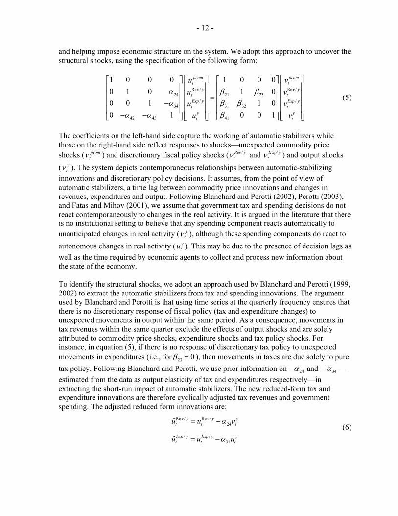
The coefficients on the left-hand side capture the working of automatic stabilizers while those on the right-hand side reflect responses to shocks—unexpected commodity price shocks ( pcom

tν ) and discretionary fiscal policy shocks ( /Rev ytν and xp/E y

tν ) and output shocks ( y

tν ). The system depicts contemporaneous relationships between automatic-stabilizing innovations and discretionary policy decisions. It assumes, from the point of view of automatic stabilizers, a time lag between commodity price innovations and changes in revenues, expenditures and output. Following Blanchard and Perotti (2002), Perotti (2003), and Fatas and Mihov (2001), we assume that government tax and spending decisions do not react contemporaneously to changes in the real activity. It is argued in the literature that there is no institutional setting to believe that any spending component reacts automatically to unanticipated changes in real activity ( y

tν ), although these spending components do react to autonomous changes in real activity ( y

tu ). This may be due to the presence of decision lags as well as the time required by economic agents to collect and process new information about the state of the economy. To identify the structural shocks, we adopt an approach used by Blanchard and Perotti (1999, 2002) to extract the automatic stabilizers from tax and spending innovations. The argument used by Blanchard and Perotti is that using time series at the quarterly frequency ensures that there is no discretionary response of fiscal policy (tax and expenditure changes) to unexpected movements in output within the same period. As a consequence, movements in tax revenues within the same quarter exclude the effects of output shocks and are solely attributed to commodity price shocks, expenditure shocks and tax policy shocks. For instance, in equation (5), if there is no response of discretionary tax policy to unexpected movements in expenditures (i.e., for 23 0β = ), then movements in taxes are due solely to pure tax policy. Following Blanchard and Perotti, we use prior information on 24 34 and α α− − —estimated from the data as output elasticity of tax and expenditures respectively—in extracting the short-run impact of automatic stabilizers. The new reduced-form tax and expenditure innovations are therefore cyclically adjusted tax revenues and government spending. The adjusted reduced form innovations are:

Re / Re /

24

/ /34

v y v y yt t t

Exp y Exp y yt t t

u u u

u u u

α

α

= −

= −

%

%

(6)

- 13 -

Combining equation (4) - (6) and with further manipulations, the structured system estimated is of the following form:

Re / Re /

//

1 2 3

1 0 0 01 0

1 01

pcomt pcom

tv y v y

t tExp y

Exp y tt y

y tt

uv

u vv

uv

u

α βγ χθ θ θ

⎡ ⎤⎡ ⎤⎡ ⎤⎢ ⎥⎢ ⎥⎢ ⎥⎢ ⎥⎢ ⎥⎢ ⎥⎢ ⎥ =⎢ ⎥⎢ ⎥⎢ ⎥⎢ ⎥⎢ ⎥⎢ ⎥ ⎢ ⎥⎣ ⎦ ⎣ ⎦⎢ ⎥⎣ ⎦

%

%

(7)

It is easy to show, using equations (5)-(7) that 21 23 31 32 1 42 43 21 43 31 2 42 43 32 3 42 23 43, , , , , and .α β β β γ β χ β θ α α β α β θ α α β θ α β α= = = = = + + = + = +

The coefficients in the final form of the system as represented in equation (7) can be interpreted as follows:

• commodity price shocks are strictly exogenous;

• α indicates the response of government revenues to unanticipated commodity price shocks, whileβ measures the response of revenues to discretionary expenditure decisions;

• government expenditures respond to both commodity and revenue shocks—the strengths of the responses are indicated by the coefficients andγ χ respectively;

• cyclically-adjusted revenues and expenditures do not respond to unanticipated output shocks within the same quarter (simply because the cyclical components of these revenues and expenditure have been extracted away using the filters indicated in equation (6)); and

• output responds contemporaneously to unanticipated commodity price shocks and discretionary revenue and expenditure policy shocks—the magnitude of the responses are given by 1 2 3, andθ θ θ , respectively. Discretionary revenue and expenditure decisions affect output only indirectly, through the autonomous relationship between output, revenues and expenditures as indicated in equation (5)—in fact, 2 3andθ θ are functions of the autonomous responses of output to revenues and expenditures ( 42 43andα α , respectively), the response of revenues to discretionary expenditure shocks ( β ), and the response of expenditures to discretionary revenue shocks ( χ ), with

2 42 43θ α α χ= + and 2 42 43θ α β α= + .

The system represented in equation (7) has 11 unknowns—7 parameters and 4 variances to be estimated using the ( 1) / 2n n + (which equals 10) variances and co-variances of the estimated reduced-form. Thus, without further restrictions, the system is unidentified. In all

- 14 -

our estimations, we set the initial number of lags in the reduced-form VAR to 6 quarters and systematically reduce these (using the Schwartz information criteria and the Akaike information criteria) until an optimal lag length is obtained. While the literature suggests that commodity prices are nonstationary, and our preliminary investigations of the data confirm this, the specific form of the data generation process is not well established. We are aware that knowledge of the form of such shocks can serve as essential input into policy design to dampen the effects of external shocks. For instance, if commodity price innovations are entirely cyclical, commodity exporting countries can benefit from stabilization policies (such as a commodity price stabilization scheme), while these schemes may not work successfully in the context of unit roots in the underlying data generation process for commodity prices (see Deaton, 1992, for example). In this paper, however, we are more concerned about the impact of commodity price changes on fiscal performance than on the nature of the data generation process for commodity prices per se. We are therefore agnostic about the data generation process of commodity prices, and allow this to be determined by the VAR process. We adopt two broad tax regimes to help identify the economically meaningful shocks in our system: 1. Pure Tax Regime. This regime is characterized by weak exogeneity of government spending decisions on tax revenues ( 0β = ). Two versions of this model are estimated. The first version is where both tax revenues and government spending decisions have immediate effects on output (Model I A: 0β = , exactly identified model). Under the second version, both decisions do not have immediate effects on output (Model I B: 0β = and 2 3 0θ θ= = , an over-identified model). 2. Expenditure-Induced Tax Regime: Under this regime, expenditure decisions are taken without any contemporaneous feedback or considerations for tax performance (i.e. where 0χ = ), whereas tax decisions take into account the expenditure shocks. Just as under the pure tax effort regime, we consider two alternative situations— immediate effect of tax and expenditure decisions on output (Model III: 0χ = , exactly-identified model), and the absence of these contemporaneous relationships (Model IV: 0χ = and 2 3 0θ θ= = , an over-identified model). In terms of political economy, the pure tax regime implies that tax decisions are made prior to and independent of expenditure decisions, while the expenditure-induced tax regime assumes subordination of tax decisions to spending programs.

- 15 -

IV. EMPIRICAL RESULTS

A. Effects of Commodity Price Shocks

1. Contemporaneous Effects of Shocks

Table 2 presents estimates of the contemporaneous effects of commodity price shocks on innovations in fiscal aggregates under alternative fiscal regimes. In particular, the table indicates (i) the magnitude and significance of the impact of commodity price shocks on tax innovations; (ii) varying impact and significance of expenditure shocks on tax innovations, and (iii) the importance of commodity price shocks, and discretionary fiscal policy shocks on output. It also presents information on the statistical credibility of the differentiation within each broad fiscal regime—in short, the significance of the over-identifying restrictions. The results indicate a generally significant positive impact of commodity price shocks on revenue/GDP innovations (α ). In addition, expenditure/GDP innovations increase in response to commodity price shocks and discretionary tax policy shocks. In all the countries, except Kazakhstan, we find positive and significant responses of revenue/GDP innovations to commodity price shocks. Even in the case of Kazakhstan, the estimates have the correct signs, although they are not statistically significant. Further, these results are largely independent of fiscal regimes, except in Tajikistan where the responses differ significantly between fiscal regimes—they jump from around 0.7 under the pure tax regime to 3.0 under the expenditure-induced tax regime. The estimated contemporaneous impact of commodity price shocks on revenue/GDP innovations are particularly strong for Russia where a one percent increase in commodity prices results in an estimated 0.9 percent increase in revenue/GDP innovations. For the Kyrgyz Republic, the estimated responses are around 0.5 under both tax regimes. This seeming invariance of the response of revenue/GDP innovations to commodity price shocks across tax regimes could be due to either of two factors—improper specification of the data generation process or the tax treatment of oil extraction and petroleum trade in practice in the oil-exporting countries and of commodity trade in the non-oil-exporting countries. Regarding the response of expenditure/GDP innovations, the results indicate a significant and positive contemporaneous effect of commodity price shocks—the estimate ofγ is significant across tax regimes in all the countries of our sample, except under the pure tax regime in Kazakhstan. The responses are generally invariant to changes in fiscal regimes, and the increase in expenditure/GDP innovations across tax regimes to a 1 percent shock to the commodity price is around 0.5 percent in Russia and the Kyrgyz Republic. Again, for Tajikistan, the response is lower (averaging 0.5 percent) under the expenditure-induced tax regime than under the pure tax regime (averaging 1.3 percent). The response is insignificant and lowest in Kazakhstan— as the country has only recently started exploiting its natural oil resource, discretionary spending has probably mainly dominated the recent patterns, and hence its difficulty to find a robust relationship. Kazakhstan has also been very prudent in its expenditure policies, at least through end 2003. For all the countries, the estimate of χ indicates a positive response of expenditures to discretionary tax increases.

- 16 -

The results for the within-quarter response of output reveal the following: (i) while positive commodity price shocks tend to increase output in the oil-exporting countries and the Kyrgyz Republic, these shocks reduce output significantly in Tajikistan; (ii) discretionary revenue shocks generally display characteristic Keynesian-type effects—where tax increases reduce output—with the tax multiplier averaging –0.3 in Russia; but (iii) output response to expenditure shocks display mixed results, possibly reflecting inadequate variation in discretionary expenditures after excluding the autonomous expenditure component. The estimated negative effects of commodity price increases in the Kyrgyz Republic and Tajikistan are explained by the inclusion of oil in the composite commodity price indices used in the analysis on these countries. Similar growth effects for oil-importing countries have been found by earlier studies (Jimenez-Rodriguez and Sanchez (2004). By excluding oil from the price index, we find that commodity price booms tend to be associated with increases in nominal output4. Except in the case of Tajikistan, the likelihood ratio test for equality between the two models could not reject the null hypothesis at the 5 percent significant level, suggesting that each fiscal regime could be represented by one model. Thus, in what follows, we limit our discussions to only Model I (representing the pure tax regime) and Model III (representing the expenditure-induced tax regime). This means that, while we accept equality of models within tax regimes, we leave the significance of the sequencing of expenditure and tax decisions to be statistically determined, contrary to the specification adopted by Blanchard and Perotti (1999). This paper extends the Blanchard and Perotti approach, and tests for differences in responses to commodity price shocks across tax regimes, a distinction that was not made in Blanchard and Perotti.

4 These results underscore the need for further research, especially on the relative importance of the channels through which symmetric and non-symmetric commodity price shocks affect output.

- 17 -

Table 2. Structural Parameter Estimates 1/

Panel 1: Kyrgyz Republic (1995:01-2004:04, # of lags = 4) Panel 2: Tajikistan (1996:01-2004:04, # of lags = 3)

Parameters Model I Model II Model III Model IV Parameters Model I Model II Model III Model IV

α 0.444 0.444 0.467 0.467 α 0.675 0.637 3.018 3.018(0.182) (0.182) (0.191) (0.193) (0.207) (0.203) (0.963) (0.963)

β 0.333 0.333 β 4.631 4.631(0.176) (0.176) (0.813) (0.813)

γ 0.573 0.573 0.543 0.543 γ 1.868 0.682 0.530 0.530(0.199) (0.191) (0.197) (0.190) (0.696) (0.214) (0.194) (0.194)

χ 0.333 0.347 χ 3.460 0.296(0.176) (0.176) (0.618) (0.052)0.430 0.406 0.430 0.423 -5.894 -6.915 -7.179 -6.216

(0.184) (0.180) (0.184) (0.180) (2.166) (2.560) (2.656) (2.301)-0.158 -0.177 -10.692 0.578(0.169) (0.169) (1.916) (0.198)0.087 0.088 0.033 0.032 -3.083 -13.191 -13.684 -11.849

(0.167) (0.167) (0.169) (0.167) (0.556) (2.269) (2.355) (2.039)

Lilkelihood ratio test for over-dentification Lilkelihood ratio test for over-dentification

0.876 1.750 91.136 9.791Significance level 0.349 0.186 Significance level 0.000 0.000

Panel 3: Kazakhstan (1994:01-2004:02, # of lags = 3) Panel 4: Russia (1994:02-2004:02, # of lags = 4)

Parameters Model I Model II Model III Model IV Parameters Model I Model II Model III Model IV

α 0.018 0.018 0.042 0.042 α 0.859 0.859 0.886 0.886(0.160) (0.160) (0.374) (0.374) (0.226) (0.226) (0.233) (0.233)

β 2.1123 2.113 β 0.255 0.255 (0.374) (0.374) (0.177) (0.177)

γ 0.318 0.318 0.136 0.136 γ 0.516 0.514 0.500 0.500(0.378) (0.381) (0.162) (0.162) (0.198) (0.195) (0.192) (0.192)

χ 2.1123 2.1323 χ 0.2551 0.164(0.374) (0.375) (0.177) (0.167)0.085 0.085 0.085 0.082 0.400 0.381 0.400 0.386

(0.168) (0.167) (0.168) (0.161) (0.200) (0.190) (0.200) (0.193)0.0765 0.2941 -0.3505 -0.2709(0.167) 0.1669 (0.188) (0.178)-0.2892 -2.899 -0.546 -0.052 -0.278 -0.293 -0.356 -0.344(0.167) (0.167) (0.167) (0.160) (0.178) (0.179) (0.188) (0.181)

Lilkelihood ratio test for over-dentification Lilkelihood ratio test for over-dentification

0.210 3.235 3.671 2.407Significance level 0.647 0.072 Significance level 0.055 0.121

Notes:1/ Figures in parethesis are estimated standard errors. The lilelihood ratio test for over-identification is derived under the null hypothesis of equality of the two models under each fiscal regime.

Pure Tax Regime Expenditure-Induced Tax Regime Pure Tax Regime Expenditure-Induced Tax Regime

Pure Tax Regime Expenditure-Induced Tax RegimePure Tax Regime Expenditure-Induced Tax Regime

to ty tp tm

0β = 0β =

1θ

2θ

3θ

0χ = 0χ =

2 0θ = 2 0θ =to ty tp tm

0β = 0β =

1θ

2θ

3θ

0χ = 0χ =

2 0θ = 2 0θ =

to ty tp tm

0β = 0β = 0χ = 0χ =2 0θ = 2 0θ =

to ty tp tm

0β = 0β = 0χ = 0χ =2 0θ = 2 0θ =

1θ

2θ

3θ

1θ

2θ

3θ

2 (1)χ 2 (1)χ

2 (1)χ2 (1)χ

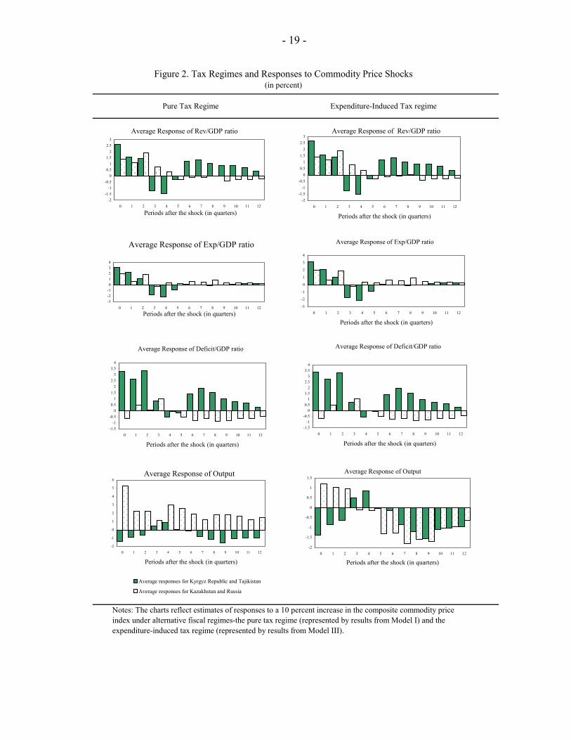
2. Dynamic Effects of Commodity Price Shocks Turning to the estimated impulse-response functions, we focus on the dynamic effects of identified commodity price shocks under both fiscal regimes. The response variables of interest are the revenue/GDP, the expenditure/GDP and the fiscal balance/GDP ratios. All the simulations are performed by considering a 1 percent transitory shock to the commodity price index and its impact on the fiscal aggregates over 12 quarters following the shock. The

- 18 -

results in Figure 2 are the estimated average dynamic responses for the oil-exporting countries (Kazakhstan and Russia) and the non-oil commodity-exporting countries (the Kyrgyz Republic and Tajikistan). The results indicate that, following a 1 percent shock to the oil price (in the case of the oil-exporting countries), revenues increase leading to budget surpluses. For the non-oil-exporting countries, the increase in the composite commodity price index leads to increases in revenues and expenditures, but also increases the budget deficit. This latter result reflects the incremental cost of oil imports on the budget, leading to budget deficits despite the increases in revenues in response to increases in the prices of their export commodities. The overall change in the fiscal balance for the two groups of countries seems more pronounced under the expenditure-induced tax regime than under the pure tax regime (i.e., under Model I, where tax policy is assumed independent of, and in advance of , expenditure decisions).5 This finding is partly explained by the long-term rigidity of expenditures even as commodity price increases dissipate. Output responses differ across fiscal regimes. When tax policy leads and is independent of expenditure decisions (as under the pure tax regime), output volatility is lower, for both groups of countries than when expenditure decisions are taken in anticipation of tax receipts (the expenditure-induced tax regime). Again, whereas the positive oil price shock increases output in the oil-exporting countries, the composite commodity price shocks in the non-oil exporting countries reduce output because of the inclusion of oil prices in the composite index. An alternative specification of the commodity price index (where oil prices are excluded from the index) in the analysis on Tajikistan and the Kyrgyz Republic yields an increase in output. Our untested hypothesis is that the decline in output in each of the two countries—the Kyrgyz Republic and Tajikistan—varies with the degree of oil-intensity in each country and the volatility of oil prices. Thus, oil price increases lead to output declines in non oil-exporting countries in our sample, while the oil-exporting countries reap gains in terms of output expansion.

5 The average responses shown in the figure blurs the differences between responses across tax regimes. Country-specific responses, not reported in this paper, display more distinct variations across tax regimes. In Figure 2, the differences between responses across tax regimes are more pronounced for output than for the fiscal aggregates. Intuitively, this result is mainly due to the additional effects of changes in taxes and spending on output (through

2θ and 3θ in equation 7 ) following the commodity price shock.

- 19 -

Expenditure-Induced Tax regimePure Tax Regime

Figure 2. Tax Regimes and Responses to Commodity Price Shocks(in percent)

Notes: The charts reflect estimates of responses to a 10 percent increase in the composite commodity price index under alternative fiscal regimes-the pure tax regime (represented by results from Model I) and the expenditure-induced tax regime (represented by results from Model III).

Average Response of Rev/GDP ratio

-2-1.5

-1-0.5

00.5

11.5

22.5

3

0 1 2 3 4 5 6 7 8 9 10 11 12

Periods after the shock (in quarters)

Average Response of Rev/GDP ratio

-2-1.5

-1-0.5

00.5

11.5

22.5

3

0 1 2 3 4 5 6 7 8 9 10 11 12


Average Response of Exp/GDP ratio

-3-2-101234

0 1 2 3 4 5 6 7 8 9 10 11 12


Average Response of Exp/GDP ratio

-3

-2

-1

0

1

2

3

4

0 1 2 3 4 5 6 7 8 9 10 11 12


Average Response of Deficit/GDP ratio

-1.5-1

-0.50

0.51

1.52

2.53

3.54

0 1 2 3 4 5 6 7 8 9 10 11 12


Average Response of Deficit/GDP ratio

-1.5-1

-0.50

0.51

1.52

2.53

3.54

0 1 2 3 4 5 6 7 8 9 10 11 12


Average Response of Output

-2

-1

0

1

2

3

4

5

6

0 1 2 3 4 5 6 7 8 9 10 11 12


Average responses for Kyrgyz Republic and Tajikistan

Average responses for Kazakhstan and Russia

Average Response of Output

-2

-1.5

-1

-0.5

0

0.5

1

1.5

0 1 2 3 4 5 6 7 8 9 10 11 12


- 20 -

Further inspection of the country-specific estimates of the impulse response functions reveals trends broadly consistent with the macroeconomic profile of commodity-producing countries. Specifically, in response to a positive commodity price shock, we observe a rise in output during the first year of the shock. After approximately four quarters, the output response reaches its peak and reverts back to its original level, and in the long run, the effects of the positive commodity price shock on output disappear.

B. The Odds on Fiscal Performance

The estimated model is used to generate stochastic simulations to assess the likelihood of exceeding fiscal floors and ceilings (in the case of the PRGF countries, Kyrgyz Republic and Tajikistan) and of a worsening of the fiscal stance (in the case of the non-PRGF countries, Kazakhstan and Russia) over the forecast horizon. Each stochastic simulation generates a hypothetical response path for the variables of the model following a positive shock to the commodity price index. These hypothetical paths are functions of two determinants— structural disturbances to the economy and the propagation mechanism of the economy, which are characterized by the specifications for each country under each fiscal regime. The structural VAR simulation procedure used in the paper is similar to the methodology used by Dalsgaard and de Serres (1999). Unlike Dalsgaard and de Serres, who use Monte Carlo simulations, we adopt a bootstrapping approach with 2,000 replications of the estimated SVAR (see Runkle, 1986, for instance, for a description of this procedure)6 to simulate impulse-responses7 that are further analyzed in determining (i) the dynamic behavior (in the forecast horizon) of revenues, expenditures and fiscal balances at

6 The bootstrapping procedure draws error terms from the set of estimated residuals, generates the variables of the VAR using the estimated coefficients and re-runs the VAR a number of times (in our case, 2,000 times). From the results of the re-runs, we can derive distributions for the impulse-responses and make inferences about the dynamic behavior of the variables of the VAR following a shock to a pre-specified variable. For instance, the estimated impulse-responses reported in this paper are the median responses derived from 2,000 replications of the SVAR. In addition, we are able to infer from the re-runs the likelihood of estimated responses exceeding some pre-determined levels—this yields the probabilities that we discuss in the next section. We also infer the level of the responses at any given (say, 1α ) significance level, yielding the expression “ 1α –significance level ” of these responses.

7 This approach is widely used in the SVAR literature to estimate confidence bands for simulated impulse-responses. The approach assumes, however, that the impulse-responses are independently distributed through time, which in a strict econometric sense is not precise. Hence the confidence bands should not be interpreted as confidence intervals, but rather as indications of uncertainty around parameter estimates. This is precisely how we use the simulated bands in this paper—to derive probabilities of exceeding fiscal targets and the ” 1α –significance levels” of the relevant fiscal variables.

- 21 -

the 1α − significance level, and (ii) the probability of exceeding specified revenue, expenditure and deficit/surplus baseline or targets—following a 1 percent commodity price shock. The simulations underlying the likely levels of the fiscal aggregates at a given significance level show fluctuations of these aggregates around their trend values in response to unexpected commodity price shocks. The estimated structural VAR is simulated 2,000 times and cumulative distributions are derived for the estimated impulse-responses under each tax regime over the forecast horizon, k. Figure 3 shows an example of probability distributions of the responses of the revenue/GDP ratio and the expenditure/GDP ratio over the forecast horizon, following a one percent positive shock to the commodity price index—the responses of the fiscal balance are derived from these two. For illustrative purposes, the target/baseline revenue and expenditure ratios in Figure 3 are set at 5 percent. The lines k = 0, k = 4, k = 8, and k = 12, indicate the probability distribution of the fiscal ratios (revenue/GDP ratio and expenditure/GDP ratio as the case may be) k-quarters after a one percent positive commodity price shock. For instance, the k = 0 line in the revenue panel indicates that the probability of exceeding the revenues baseline following a positive one percent commodity price shock is about 80 percent (i.e., 100 minus 20 percent). A corresponding estimate of the probability of exceeding the expenditure baseline or ceiling at the zero horizon (i.e., along line k = 0) would be 90 percent (i.e., 100 minus 10 percent). The various k-lines indicate, therefore, the probabilities of exceeding fiscal floors or ceilings (or baseline fiscal ratios) at various horizons following the positive price shock. The figure also shows the likely levels of the fiscal aggregates at the 1α − significance level at each horizon. These levels are given by the points of intersection between the vertical line labeled “5-percent significance level” and the estimated probabilities at each forecast horizon (k). The figure suggests for instance, that, at the 5-percent significance level, the revenue ratio is likely to be above 5 percent of GDP for all k quarterly forecast periods following a one percent positive commodity price shock. This approach is used to estimate the 1α − significance level of fiscal aggregates and probabilities of fiscal over-performance relative to the baseline or target.

- 22 -

Source: Authors' simulations, based on estimated structural VAR and impulse-responses.

Figure 3. Illustrative Probability Distribution of Fiscal Aggregates

-10

0

10

20

30

40

1 2.5

5 10 20 25 33.3

50 66.7

75 80 90 95 97.5

99 99.5

99.75

99.9

Max.

Percentiles

Bas

elin

e pl

us E

stim

ated

Res

pons

es (i

n pe

rcen

t of G

DP)

k = 0

k = 4k = 8

k = 12

Baseline/Target revenue-to-GDP ratio

5-percent significance level

Revenue/GDP Ratio k Periods After a 1 Percent Commodity Price Shock

-10

0

10

20

30

40

1 2.5

5 10 20 25 33.3

50 66.7

75 80 90 95 97.5

99 99.5

99.75

99.9

Max.

Percentiles

Bas

elin

e pl

us E

stim

ated

Res

pons

es (i

n pe

rcen

t of G

DP)

k = 0k = 4k = 8k = 12 5-percent significance level

Baseline/Target expenditure-to-GDP ratio

Expenditure/GDP Ratio k Periods After a 1 Percent Commodity Price Shock

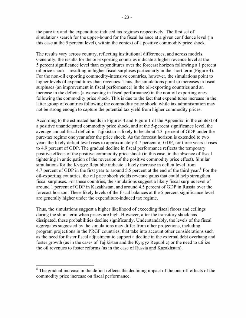
1. 1α − significance Levels of Fiscal Aggregates The first characterization of the responses of the fiscal aggregates to commodity price shocks show how the tax and expenditure aggregates would fluctuate around their trend values in response to a positive unexpected transitory commodity price shock. The simulations provide, therefore, a basis for determining the size of the buffer required to protect against unexpected shocks driving these fiscal aggregates outside a specified band. The results of these simulations are presented in Figures 4 and 5. Again, Model I and Model III represent

- 23 -

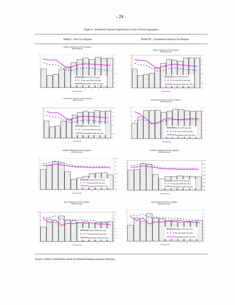
the pure tax and the expenditure-induced tax regimes respectively. The first set of simulations search for the upper-bound for the fiscal balance at a given confidence level (in this case at the 5 percent level), within the context of a positive commodity price shock. The results vary across country, reflecting institutional differences, and across models. Generally, the results for the oil-exporting countries indicate a higher revenue level at the 5 percent significance level than expenditures over the forecast horizon following a 1 percent oil price shock—resulting in higher fiscal surpluses particularly in the short term (Figure 4). For the non-oil exporting commodity-intensive countries, however, the simulations point to higher levels of expenditures than revenues. Thus, the simulations point to increases in fiscal surpluses (an improvement in fiscal performance) in the oil-exporting countries and an increase in the deficits (a worsening in fiscal performance) in the non-oil exporting ones following the commodity price shock. This is due to the fact that expenditures increase in the latter group of countries following the commodity price shock, while tax administration may not be strong enough to capture the potential tax yield from higher commodity prices. According to the estimated bands in Figures 4 and Figure 1 of the Appendix, in the context of a positive unanticipated commodity price shock, and at the 5-percent significance level, the average annual fiscal deficit in Tajikistan is likely to be about 4.3 percent of GDP under the pure-tax regime one year after the price shock. As the forecast horizon is extended to two years the likely deficit level rises to approximately 4.7 percent of GDP, for three years it rises to 4.9 percent of GDP. The gradual decline in fiscal performance reflects the temporary positive effects of the positive commodity price shock (in this case, in the absence of fiscal tightening in anticipation of the reversion of the positive commodity price effect). Similar simulations for the Kyrgyz Republic indicate a likely increase in deficit level from 4.7 percent of GDP in the first year to around 5.5 percent at the end of the third year.8 For the oil-exporting countries, the oil price shock yields revenue gains that could help strengthen fiscal surpluses. For these countries, the simulations suggest a likely fiscal surplus level of around 1 percent of GDP in Kazakhstan, and around 4.5 percent of GDP in Russia over the forecast horizon. These likely levels of the fiscal balances at the 5 percent significance level are generally higher under the expenditure-induced tax regime. Thus, the simulations suggest a higher likelihood of exceeding fiscal floors and ceilings during the short-term when prices are high. However, after the transitory shock has dissipated, these probabilities decline significantly. Understandably, the levels of the fiscal aggregates suggested by the simulations may differ from other projections, including program projections in the PRGF countries, that take into account other considerations such as the need for faster fiscal adjustment to support a decline in the external debt overhang and foster growth (as in the cases of Tajikistan and the Kyrgyz Republic) or the need to utilize the oil revenues to foster reforms (as in the case of Russia and Kazakhstan).

8 The gradual increase in the deficit reflects the declining impact of the one-off effects of the commodity price increase on fiscal performance.

- 24 -

Source: Authors' simulations, based on estimated impulse-response functions.

Figure 4. Simulated 5-percent Significance Levels of Fiscal Aggregates

Model I - Pure Tax Regime Model III - Expenditure-Induced Tax Regime

Tajikistan. Simulated Levels of Fiscal Aggregates Model I (in percent)

0

1

2

3

4

5

6

7

8

9

10

1 2 3 4 5 6 7 8 9 10 11 12

Forecast Horizon (k)

0.9

0.95

1

1.05

1.1

1.15

1.2

1.25

Deficit-GDP ratio (rhs)

Revenue-GDP ratio (lhs)

Expenditure-GDP ratio (lhs)

Tajikistan: Simulated Levels of Fiscal Aggregates Model III (in percent)

0

1

2

3

4

5

6

7

8

9

10

1 2 3 4 5 6 7 8 9 10 11 12


0.9

0.95

1

1.05

1.1

1.15

1.2

1.25




Kyrgyz Republic: Simulated Levels of Fiscal Aggregates Model III (in percent)

0

2

4

6

8

10

12

14

1 2 3 4 5 6 7 8 9 10 11 12


0

0.2

0.4

0.6

0.8

1

1.2

1.4

1.6




Kyrgyz Republic: Simulated Levels of Fiscal Aggregates Model I (in percent)

0

1

2

3

4

5

6

7

8

9

10

1 2 3 4 5 6 7 8 9 10 11 12


0.9

0.95

1

1.05

1.1

1.15

1.2

1.25




Kazakhstan: Simulated Levels of Fiscal Aggregates Model I (in percent)

0

1

2

3

4

5

6

7

8

9

10

1 2 3 4 5 6 7 8 9 10 11 12


0.205

0.21

0.215

0.22

0.225

0.23

0.235

0.24

0.245

Surplus-GDP ratio (rhs)



Kazakhstan: Simulated Levels of Fiscal Aggregates Model III (in percent)

0

1

2

3

4

5

6

7

8

9

10

1 2 3 4 5 6 7 8 9 10 11 12


0.205

0.21

0.215

0.22

0.225

0.23

0.235

0.24

0.245




Russia: Simulated Levels of Fiscal Aggregates Model I (in percent)

0

1

2

3

4

5

6

7

8

9

10

1 2 3 4 5 6 7 8 9 10 11 12


0

0.2

0.4

0.6

0.8

1

1.2

1.4

1.6

1.8




Russia: Simulated Levels of Fiscal Aggregates Model III (in percent)

0

1

2

3

4

5

6

7

8

9

10

1 2 3 4 5 6 7 8 9 10 11 12


0

0.2

0.4

0.6

0.8

1

1.2

1.4

1.6

1.8




- 25 -

2. Probability of Exceeding Fiscal Floors and Ceilings The second set of simulations estimates probabilities of exceeding fiscal floors and ceilings (in the case of Kyrgyz Republic and Tajikistan) or performing worse than the recent trend (in the case of the non-PRGF oil-exporting countries—Kazakhstan and Russia). These probabilities are conditional on the estimated responses to a 1 percent positive shock to the commodity price index. A priori, one would expect the probability of over-performing revenue floors to be higher under the expenditure-induced tax regime than under the pure tax regime, as the former regime benefits from additional revenue boost from autonomous expenditure increases. The simulation results confirm this belief, but this particular sequencing of tax and expenditure policy—the expenditure-induced tax regime—does not necessarily yield higher/lower likelihoods of exceeding fiscal surpluses/deficits, as its is also generally associated with higher expenditures than under the pure tax regime (Figure 5). In general, fiscal floors and ceilings are easily exceeded during the first year of the positive commodity price shock. However, this performance deteriorates shortly after the transitory shock. In the long run, the expenditure-induced tax regime yields higher probabilities of exceeding deficit ceilings in the non-oil exporting countries (Kyrgyz Republic and Tajikistan) and lower likelihoods of exceeding the floors on the fiscal surplus (at least in the case of Kazakhstan) than under the pure tax regime. This is mainly because, expenditures that get entrenched during the commodity price boom periods are adjusted slowly once the commodity price declines. For Tajikistan, immediately after the price shock, the probability of over-performing on revenues is high for a short period of time, leading to a corresponding increase in expenditures. However, as spending is not immediately adjusted following the cessation of the temporary increase in commodity prices, the likelihood of meeting the fiscal deficit deteriorate. After a while, due to growth effects and eventual adjustment of spending, it becomes more likely to meet the fiscal targets. The expenditure-induced tax regime yields higher probabilities in the second and third years following the commodity price shock. For the Kyrgyz Republic, the odds against exceeding the deficit ceiling rise sharply to between 0.9 and 1 in the first quarter after the price shock, but decline to between zero and 0.1 in subsequent quarters—again, the expenditure-induced tax regime yields higher probabilities of exceeding the ceiling on the fiscal deficit, although it also yields higher probabilities of exceeding the tax floors. Likewise for Kazakhstan and Russia, the probability of exceeding the fiscal surplus (i.e. the likelihood of improving fiscal performance relative to the most recent trend) is higher in the long run under the expenditure-induced tax policy than under the pure tax regime. For Kazakhstan, while the probabilities of exceeding the revenue target and the expenditure target decline, in particular, in the second to fourth quarters after the transitory commodity price shock, the probability of exceeding the floor on the fiscal surplus remains flat under both tax regimes. In the long run, however, the probability of exceeding the pre-specified expenditure ceiling rises faster than that of exceeding the revenue floor, leading to a decline in the probability of exceeding the fiscal surplus, particularly under the expenditure-induced tax regime. In Russia, however, the opposite seems to be the case—the expenditure-induced tax regime yields higher probabilities of exceeding the surplus—and the simulated odds on

- 26 -

fiscal performance do not vary much across tax regimes. This invariance of fiscal performance across tax regimes could be due to the lack of statistical evidence to reject the null hypothesis of equality between the two model variants (Table 1).

Figure 5. Tax Regimes and Probabilities of Exceeding Pre-Specified Fiscal Ratios

Source: Author's bootstrapping simulations, based on the estimated Structural VAR.

Tajikistan: Est imated Probabilit ies of Exceeding Tax Floors

0

20

40

60

80

100

120

0 1 2 3 4 5 6 7 8 9 10 11 12


( M odel I Prob: t > T )

( M odel III Prob: t > T )

Tajikistan: Est imated Probabilit ies of Exceeding Expenditure Ceilings

0

20

40

60

80

100

120

0 1 2 3 4 5 6 7 8 9 10 11 12


( M odel I Prob. : g > G)

( M odel III Prob. : g > G)

Tajikistan: Est imated Probabilit ies of Exceeding Deficit Ceilings

-20

0

20

40

60

80

100

120

0 1 2 3 4 5 6 7 8 9 10 11 12


(M odel IProb.:def icit > D)

(M odel IIIProb.:def icit > D)

Kyrgyz Republic: Est imated Probabilit ies of Exceeding Tax Floors

0

20

40

60

80

100

120

0 1 2 3 4 5 6 7 8 9 10 11 12


( M odel I Prob: t >T )

( M odel III Prob: t >T )

Kyrgyz Republic: Est imated Probabilit ies of Exceeding Expenditure Ceilings

0

10

20

30

40

50

60

70

80

90

100

0 1 2 3 4 5 6 7 8 9 10 11 12




Kyrgyz Republic: Est imated Probabilit ies of Exceeding Deficit Ceilings

-20

0

20

40

60

80

100

120

0 1 2 3 4 5 6 7 8 9 10 11 12


(M odel I Prob.:def icit > D)

(M odel III Prob.:def icit > D)

- 27 -

Figure 5 (concluded). Tax Regimes and Probabilities of Exceeding Pre-Specified Fiscal Ratios

Source: Author's bootstrapping simulations, based on estimated Structural VAR.

Kazakhstan: Est imated Probabilit ies of Exceeding Tax Floors

0

20

40

60

80

100

120

0 1 2 3 4 5 6 7 8 9 10 11 12




Russia: Est imated Probabilit ies of Exceeding Tax Fllors

0

20

40

60

80

100

120

0 1 2 3 4 5 6 7 8 9 10 11 12




Kazakhstan: Est imated Probabilit ies of Exceeding Expenditure Ceilings

0

20

40

60

80

100

120

0 1 2 3 4 5 6 7 8 9 10 11 12




Russia: Est imated Probabilit ies of Exceeding Expenditure Ceilings

0

20

40

60

80

100

120

0 1 2 3 4 5 6 7 8 9 10 11 12




Kazakhstan: Est imated Probabilit ies of Exceeding Surplus Floors

0

20

40

60

80

100

120

0 1 2 3 4 5 6 7 8 9 10 11


(M odel I Prob.:surplus > S)

(M odel III Prob.:surplus > S)

Russia: Est imated Probabilit ies of Exceeding Surplus Floors

-10

0

10

20

30

40

50

60

70

80

90

0 1 2 3 4 5 6 7 8 9 10 11 12


(M odel I Prob.:surplus > S)

(M odel III Prob.:surplus > S)

- 28 -

V. CONCLUDING REMARKS

This paper estimated a standard structural VAR model, identified two broad tax regimes, and carried out simulations that generated likely levels of relevant fiscal aggregates at the 5 percent significance level and probabilities of exceeding fiscal floors and ceilings in the context of volatile commodity prices. The lessons from the simulations suggest that sequencing of expenditure and tax policies is crucial for fiscal performance. Thus, within an uncertain commodity price setup, the PRGF countries in our sample have higher probabilities of meeting their respective fiscal targets if they follow a more conservative tax regime—a pure tax regime—rather than allowing revenue targets to be determined by expenditure commitments. For the oil-producing non-PRGF countries, expenditure restraint would be beneficial when rising oil prices are transitory, as in the case analyzed in this paper, because the probability of over-performing recent trends in fiscal surpluses decline once the revenue-enhancing effects of the transitory oil price increase dissipate.

In addition to adopting a conservative tax regime even in the context of increasing commodity prices, increasing diversification of the economy will help enhance resilience (of non-oil exporting commodity-intensive small economies, in particular) to commodity price shocks. Increasing dependence of fiscal revenues on commodity prices renders public finances vulnerable to a volatile external variable that is, for the most part, largely beyond the control of policy makers. This calls for further diversifying the economy (through advancement of the private sector development agenda) to widen the tax base and enhancing tax administration, and thereby reduce the vulnerability of the economy to commodity price shocks. The high volatility of commodity prices also calls for flexibility in the design and application of medium-term budget frameworks in commodity-dependent economies. As projected revenues may possibly not be realized due to exogenous shocks, strict commitment to a medium-term budget framework could restrain the use of discretionary fiscal policy and delay the fiscal adjustment process. As increases in spending are usually difficult to adjust once they get entrenched, significant reductions in tax revenues could result in higher fiscal deficits (or payment arrears) that may compromise macroeconomic stability.

- 29 -

REFERENCES

Fatás, Antonio, and Ilian Mihov, 2001, “Government Size and Automatic Stabilizers: International and International evidence, ” Journal of International Economics, Vol. 55, No. 1 pp. 3–28.

Barnett, Steven, and Rolando Ossowski, 2002, “Operational Aspects of Fiscal Policy in Oil-Producing Countries, ” IMF Working Paper 02/177 (Washington: International Monetary Fund).

Blanchard, Olivier, and Roberto Perotti, 1999, “An Empirical Characterization of the Dynamic Effects of Changes in Government Spending and Taxes on Output,” NBER Working Paper 7269 (Cambridge, Massachusetts: National Bureau of Economic Research).

Bernanke, Ben, 1986, “Alternative Explanations of the Money-Income Correlation,” Carnegie-Rochester Conference Series on Public Policy, Vol. 25, pp. 49–100.

Clements, Michael P., and Graham E. Mizon, 1991, “Empirical Analysis of Macroeconomic Time Series: VAR and Structural Models,” European Economic Review, Vol. 35, pp. 887–932.

Dalsgaard, Thomas, and Alain de Serres, 1999, “Estimating Prudent Budget Margins for 11 EU Countries: A Simulated SVAR Model Approach, Working Paper 216 (Paris: Organisation for Economic Cooperation and Development).

Deaton, Angus S., 1992, “Commodity Prices, Stabilization, and Growth in Africa,” Research Program in Development Studies, Discussion Paper 166 (Princeton: Princeton University)

Engel, E., and R. Valdes, 2000, “Optimal Fiscal Strategy for Oil-Exporting Countries,” IMF

Working Paper 00/118 (Washington: International Monetary Fund). Jimenez-Rodriguez, Rebeca, and Marcello Sanchez, 2004, “Oil Price Shocks and Real GDP

Growth: Empirical Evidence for Some OECD Countries,” Working Paper Series No. 362 (Frankfurt: European Central Bank).

Kumah, Francis Y., 1996, “Common Stochastic Trends in the Current Account, ” Discussion

Paper No. 84 (Tilburg: Tilburg University: Center For Economic Research).

Kumah, Francis Y., and Salifu B. Ibrahim, 1996, “Stochastic Trends and Fluctuations in the Interest Rate, Exchange Rate and the Current Account Balance, ” Economic Modelling, Vol. 13, No. 3, pp. 383–407.

Runkle, D., 1987, “Vector Autoregressions and Reality,” Journal of Business and Economic Statistics, Vol. 5, pp. 437–42.

Sims, Christopher 1986, “Are Forecasting Models Usable for Policy Analysis?” Quarterly Review of the Federal Reserve Bank of Minneapolis (Winter), pp. 2–16.

- 30 -

Sims, Christopher., James H. Stock, and Mark W. Watson, 1990, “Inference in Times Series Models with Some Unit Roots,” Econometrica, Vol. 58, pp. 113–44.

Talvi, Ernesto, and Carlos Vegh, 2000, “Tax Base Variability and Procyclical Fiscal Policy, ” NBER Working Paper No. 7499 (Cambridge, Massachusetts: National Bureau of Economic Research)

- 31 - APPENDIX

Simulated 1α -significance Levels of Fiscal Aggregates and Probabilities of Exceeding Pre-Specified Fiscal Ratios

Estimated Fiscal Aggregatesat the 5% Significance level

Estimated Probability of ExceedingSet Fiscal Targets

Figure 1. Kyrgyz Republic: Tax Regimes and Fiscal Performance

Source:Authors' estimates. The legend in the first chart applies to all the other charts.

Revenue-GDP ratio

0

2

4

6

8

10

12

14

16

1 2 3 4 5 6 7 8 9 10 11 12

Forecast Horizon (in quarters)

Model I Model II Model III Model IV

Revenue-GDP ratio

0

20

40

60

80

100

120

1 2 3 4 5 6 7 8 9 10 11 12


Expenditure-GDP ratio

0

2

4

6

8

10

12

14

16

1 2 3 4 5 6 7 8 9 10 11 12



0

10

20

30

40

50

60

70

80

90

100

1 2 3 4 5 6 7 8 9 10 11 12


Deficit-GDP ratio

0

2

4

6

8

10

12

14

16

1 2 3 4 5 6 7 8 9 10 11 12


Deficit-GDP ratio

-20

0

20

40

60

80

100

120

1 2 3 4 5 6 7 8 9 10 11 12


- 32 - APPENDIX



Figure 2. Tajikistan: Tax Regimes and Fiscal Performance


Revenue-GDP ratio

0

2

4

6

8

10

12

14

16

1 2 3 4 5 6 7 8 9 10 11 12



Revenue-GDP ratio

0

20

40

60

80

100

120

1 2 3 4 5 6 7 8 9 10 11 12



0

2

4

6

8

10

12

14

1 2 3 4 5 6 7 8 9 10 11 12



0

20

40

60

80

100

120

1 2 3 4 5 6 7 8 9 10 11 12


Deficit-GDP ratio

0.0

0.5

1.0

1.5

2.0

2.5

1 2 3 4 5 6 7 8 9 10 11 12


6

Deficit-GDP ratio

-20

0

20

40

60

80

100

120

1 2 3 4 5 6 7 8 9 10 11 12


- 33 - APPENDIX



Figure 3. Kazakhstan: Tax Regimes and Fiscal Performance


Revenue-GDP ratio

0

2

4

6

8

10

12

1 2 3 4 5 6 7 8 9 10 11 12



Revenue-GDP ratio

0

20

40

60

80

100

120

1 2 3 4 5 6 7 8 9 10 11 12



0

1

2

3

4

5

6

7

8

9

10

1 2 3 4 5 6 7 8 9 10 11 12



0

10

20

30

40

50

60

70

80

90

100

1 2 3 4 5 6 7 8 9 10 11 12


Surplus-GDP ratio

0.20

0.21

0.21

0.22

0.22

0.23

0.23

0.24

0.24

0.25

0.25

1 2 3 4 5 6 7 8 9 10 11 12


Surplus-GDP ratio

0

20

40

60

80

100

120

1 2 3 4 5 6 7 8 9 10 11 12


- 34 - APPENDIX



Figure 4. Russia: Tax Regimes and Fiscal Performance


Revenue-GDP ratio

0

2

4

6

8

10

12

14

1 2 3 4 5 6 7 8 9 10 11 12Forecast Horizon (in quarters)


Revenue-GDP ratio

0

20

40

60

80

100

120

1 2 3 4 5 6 7 8 9 10 11 12



0

1

2

3

4

5

6

7

8

9

10

1 2 3 4 5 6 7 8 9 10 11 12



0

10

20

30

40

50

60

70

80

90

100

1 2 3 4 5 6 7 8 9 10 11 12


Surplus-GDP ratio

0.0

0.2

0.4

0.6

0.8

1.0

1.2

1.4

1.6

1.8

1 2 3 4 5 6 7 8 9 10 11 12


Surplus-GDP ratio

-10

0

10

20

30

40

50

60

70

80

90

1 2 3 4 5 6 7 8 9 10 11 12


commodity price shocks and the odds on fiscal performance: a

Documents