Commitments to Save: A Field Experiment in Rural Malawi∗

Lasse Brune Department of Economics, University of Michigan

Xavier Giné Development Economics Research Group, World Bank and Bureau for Economic Analysis and Development (BREAD)

Jessica Goldberg Department of Economics, University of Maryland

Dean Yang

Ford School of Public Policy and Department of Economics, University of Michigan, Bureau for Economic Analysis and Development (BREAD), and National Bureau of Economic Research (NBER)

February 2013 Abstract We report the results of a field experiment that randomly offered Malawian smallholder farmers formal savings accounts. We tested two primary treatments, offering either: 1) “ordinary” accounts, or 2) both ordinary and “commitment” accounts. Commitment accounts allowed customers to restrict access to their own funds until a future date of their choosing. A control group was not offered any account but was tracked alongside the treatment groups. The commitment treatment led to increases in deposits at the partner bank, and over the next agricultural year caused increases in agricultural input use, crop sales, and household expenditures. The effects of the commitment treatment are not due to literally “tying the hands” of farmers, since farmers in that treatment mostly saved in ordinary accounts (rather than commitment accounts). We discuss other possible channels through which the commitment treatment’s effects may have operated, such as reduced sharing with one’s social network as well as other psychological channels. Keywords: savings, commitment, hyperbolic preferences, self-control, sharing norms, mental accounting. JEL codes: D03, D91, O16, Q14.

∗ Brune: lfbrune@umich.edu. Giné: xgine@worldbank.org. Goldberg: goldberg@econ.umd.edu. Yang:

deanyang@umich.edu. We thank Niall Keleher, Lutamyo Mwamlima and the IPA staff in Malawi; Steve Mgwadira, Mathews Kapelemera, and Webster Mbekeani of OIBM; and the OIBM management and staff of Kasungu, Mponela and Lilongwe branches. Matt Basilico and Britni Must provided excellent research assistance. We are grateful to Beatriz Armendariz, Orazio Attanasio, Oriana Bandiera, Abhijit Banerjee, Luc Behagel, Marcel Fafchamps, Maitreesh Ghatak, Marc Gurgand, Sylvie Lambert, Kim Lehrer, Rocco Macchiavello, Lou Maccini, Sharon Maccini, Marco Manacorda, Costas Meghir, Rohini Pande, Albert Park, Imran Rasul, Chris Woodruff, Bilal Zia, Andrew Zeitlin, and seminar participants at the FAI Microfinance Innovation Conference, Ohio State, London School of Economics, Warwick, Institute for Fiscal Studies, Paris School of Economics, and Oxford for helpful comments. We appreciate the support of David Rohrbach (World Bank) and Jake Kendall (Bill & Melinda Gates Foundation). We are grateful for research funding from the World Bank Research Committee and the Bill & Melinda Gates Foundation. The views expressed in this paper are those of the authors and should not be attributed to the World Bank, its executive directors, or the countries they represent.

0

1. Introduction

Recent experimental studies have found high marginal returns to capital in developing

countries in non-agricultural enterprises (de Mel, McKenzie and Woodruff, 2008; Fafchamps et

al., 2011) as well as in agriculture (Duflo, Kremer and Robinson, 2008). These high returns stand

in contrast to low utilization of modern inputs such as fertilizer in many low-income countries,

particularly in sub-Saharan Africa (World Bank, 2008).

To raise input utilization in agriculture, many developing country governments and donors

have implemented large-scale input subsidies. However, the scale of such programs takes a

heavy toll on government budgets, casting doubt on their long-term sustainability.1 Another

popular response has been the introduction of microcredit programs. In 2009, the Microcredit

Summit estimated that there were more than 3,500 microfinance institutions around the world

with 150 million clients (Daley-Harris 2009). While these outreach numbers are impressive,

microcredit today is largely devoted to non-agricultural activities (Morduch 1999; Armendariz

de Aghion and Morduch 2005) due to the substantial challenges inherent in agricultural lending.2

Given the limited supply of credit for agriculture, many donors and academics (for example,

Deaton, 1990; Robinson, 2001 and more recently the Bill and Melinda Gates Foundation) have

emphasized the potential for increasing access to formal savings.3

Low-income individuals, however, have difficulty saving in formal banking institutions.

Instead, they rely on more expensive and riskier methods to save informally (Rutherford, 2000

and Collins, Morduch, Rutherford and Ruthven, 2009). These alternatives include cash held at

home, purchases of durable assets such as livestock with risky returns, participation in ROSCAs

(rotating savings and credit associations), or the use of deposit collectors (such as susu collectors

in West Africa). 1 For example, the cost of Malawi’s large-scale fertilizer subsidy program amounted to 11 percent of the total

government budget in the 2010-11 fiscal year. 2 Giné, Goldberg, and Yang (2012) find that imperfect personal identification leads to asymmetric information

problems (both adverse selection and moral hazard) in the rural Malawian credit market. 3 Aportela (1999) uses data from an expansion of branches set up in post offices in the end of 1993. He finds

that the expansion resulted in an average increase in savings rate of 3 to 5 percentage points, with higher effects (up to 7 percentage points) for low-income individuals compared to other low-income households located in towns without the expansion. Burgess and Pande (2005) find that a policy-driven expansion of rural banking reduced poverty in India, and provide suggestive evidence that deposit mobilization and credit access were intermediating channels. Despite positive social effects, the program was discontinued in 2001 due to losses from defaults. Bruhn and Love (2009) examine the opening of bank branches in consumer durable stores in Mexico in 2002 and find an increase in the number of informal business owners by 7.6 percent, in total employment by 1.4 percent, and in average income by about 7 percent. The effects are concentrated among low income households and in municipalities with lower pre-existing bank penetration.

1

A number of explanations have been advanced for low levels of formal savings in

developing countries. Transaction costs for formal savings may be high for a variety of reasons,

including substantial distances to branches, costly and unreliable transport, and mistrust towards

formal financial institutions. In addition, financial illiteracy may prevent households from

opening accounts due to a lack of knowledge about the benefits of formal savings and lack of

familiarity with account-opening procedures (Cole, Sampson and Zia, 2011).

Psychological factors, such as impatience (a strong preference for the present over the

future) and issues of self-control (competing preferences that dictate different actions at different

times) may also lead to lower savings. There is evidence from both developed and developing

countries that self-aware individuals seek to limit their options in anticipation of future self-

control problems. Ashraf, Karlan, and Yin (2006) investigate demand for and impacts of a

commitment savings device in the Philippines and find that demand for such commitment

devices is concentrated among women exhibiting present-biased time preferences. Duflo,

Kremer and Robinson (2011) find that offering a small, time-limited discount on fertilizer

immediately after harvest has an effect on fertilizer use that is comparable to that of much larger

discounts offered later, around planting time. Giné et al. (2012) find that Malawian tobacco

farmers with present-biased preferences are more likely to revise a plan about how to use future

income, even when that plan is made under commitment.

Another potential explanation for low savings levels in rural communities is the pressure to

share income with spouses (see, e.g., Anderson and Baland 2002; Ashraf 2009; Schaner, 2012),

relatives and friends (see, e.g., Platteau, 2000; Maranz, 2001; Ligon, Thomas, and Worall, 2002;

Hoff and Sen, 2006; Baland, Guirkinger and Mali, 2011; Jakiela and Ozier, 2011). Sharing

obligations may discourage individuals from exerting effort or accumulating assets, and may

encourage them to spend resources hastily before income is dissipated through demands from

others. People who anticipate pressure to share cash with others in their social network may

spend that money quickly in order to pre-empt requests for transfers (Goldberg 2011).

An important point is that commitment devices, by tying the hands of individuals, may also

make it easier to resist demands for sharing with their social network. In other words,

commitment devices may assist with “other”-control as well as self-control problems. The

existing literature has only partially investigated whether the demand for and impact of

commitment devices is (at least in part) due to other-control problems (Hertzberg 2010).

This discussion brings to the fore three interrelated questions that are the focus of this paper.

First, does merely offering easy access to formal savings accounts improve savings and other

2

household outcomes? Second, are such impacts magnified when the savings accounts offered

have commitment features, such as an option to voluntarily restrict one’s own ability to make

withdrawals for a defined period of time? Third, if offering accounts with commitment features

leads to larger impacts, what is the underlying mechanism through which the effect operates?

To answer these questions, we implemented a field experiment among smallholder cash crop

farmers in Malawi. We are able to shed light most clearly on the first two questions. With respect

to the third question (on mechanisms of commitment impacts), we provide clear evidence against

the self-control channel, discuss some evidence on the other-control channel, and speculate on

other psychological channels that might be at work.

In our experiment, conducted in partnership with a local microfinance institution, we

randomized offers of account-opening and deposit assistance for formal savings accounts. One

randomly-selected group of farmers was simply offered assistance opening individual “ordinary”

savings accounts with standard features. This treatment sheds light on the impact of simply

facilitating access to savings accounts. To test the importance of offering accounts with

commitment features, another randomly-selected group of farmers was offered, in addition to the

“ordinary” account, a “commitment” savings account that allowed account holders to request

that funds be frozen until a specified date (e.g., until the next planting season, so that funds could

be preserved for farm input purchases). Other farmers were randomly assigned to a control group

that was surveyed but not offered assistance with opening either type of savings account. This

design allows us to test the relative impact of offering accounts with commitment features versus

offering only ordinary savings accounts.

We designed a sub-experiment to test whether pressure to share with one’s social network

reduces savings. Among farmers who were offered the savings treatments, we cross-randomized

an intervention that provided a public signal of individual savings account balances. If the public

revelation of balances induces greater pressure to share, then saving balances may be lower.4

Our findings are distinguished from those in the existing literature in two ways. First, we are

among the first to show impacts of commitment savings offers (as opposed to offers of ordinary

accounts) on important economic outcomes beyond savings.5 Previous research has often

4 Flory (2011) conducts a field experiment in rural Malawi where households in treatment villages were

encouraged to open savings accounts. He finds that transfers to poor households increase in treatment villages, perhaps because everyone in the village knew who had savings accounts and thus access to funds.

5 As a follow-up to Ashraf, Karlan, and Yin (2006), Ashraf, Karlan, and Yin (2010) show impacts of commitment account offers on female empowerment in the same Philippine experimental sample.

3

focused on the mechanical effects of savings products on levels of savings, but we have longer

run outcomes that measure economic impacts more directly. The commitment treatment had

large positive effects on a range of outcomes of interest: deposits and withdrawals at our partner

institution immediately prior to the next planting season, land under cultivation (an increase

amounting to 9.8% of the control group mean), agricultural input use in that planting (27.4%

increase over the control group mean), crop output in the subsequent harvest (21.8% increase),

and household expenditures in the months immediately after harvest (17.4% increase). While the

ordinary treatment’s effect on deposits and withdrawals was similar to that of the commitment

treatment effect, the ordinary treatment effects on agricultural inputs and subsequent outcomes

are uniformly smaller than those of the commitment treatment, and are never statistically

significantly different from zero. A joint hypothesis test finds that the impact of the commitment

account offer on the set of agricultural and expenditure outcomes is statistically significantly

larger than the effect of the ordinary account offer.

The second key contribution of this paper is to demonstrate that if an offer of commitment

savings accounts has substantial impacts (e.g., on later outcomes such as investment and

household productive output), it does not have to operate via solving individuals’ self-control

problems. The basic facts in our experiment are striking: the vast majority (89.0%) of deposits

among individuals offered commitment accounts were in ordinary as opposed to commitment

accounts. The average amount deposited in commitment accounts was about an order of

magnitude smaller than the commitment treatment’s later impact on input use. Clearly, the

commitment treatment did not have its impact solely by literally “tying the hands” of farmers by

preventing them from withdrawing money in the months prior to planting time. Impacts on total

deposits (in ordinary and commitment accounts combined), by contrast, do exceed the impact on

later reported increases in inputs, so the measured increase in inputs could have been funded by

total deposited funds (just not by the funds deposited into commitment accounts alone).

Through what other channels might the effects of the commitment treatment have operated?

We explore two alternative mechanisms. First, the commitment treatment could have helped

farmers solve “other-control” problems, by allowing them to better resist social network

demands for their savings.6 As it turns out, we do not find conclusive evidence in support of this

6 Even though only a small minority of deposits went into commitment accounts, farmers might have been able to claim to others in their social network that their funds were tied up, since the distribution of funds across ordinary and commitment accounts was not public knowledge. The cross-randomized raffle treatments awarded raffle tickets

4

hypothesis. The commitment treatment did not reduce reported transfers to other households; in

addition, the sub-experiment that created public revelation of savings balances did not lead to

lower savings as expected.7 That said, it is still possible that the commitment treatment allowed

study participants to keep funds from others within the household, or to refrain from consuming

resources early in anticipation of future requests from others (as in Goldberg 2011). We therefore

believe the other-control channel should remain an important focus in future research.

Second, the commitment treatment may have led to changes in behavior via other

psychological channels. In the commitment treatment we asked farmers to specify in advance

how much money from their crop sales they wanted to be directly deposited into their ordinary

and commitment accounts. This mere elicitation of farmers’ intentions may have influenced their

later behavior (Feldman and Lynch 1988, Webb and Sheeran 2006, Zwane et al, 2011).

Relatedly, the act of stating amounts to be deposited into commitment accounts may have

created a investment mental account (Thaler, 1990), although the accounts were not actively

labeled. Unfortunately, we can offer no direct evidence to support or contradict that such

psychological channels may have been at work. Future research should prioritize investigation of

these and potentially other psychological channels.

This paper contributes to the burgeoning literature on the effects of formal savings accounts,

and in particular of making offers of commitment savings. Dupas and Robinson (2012a) offer

ordinary savings accounts to Kenyan urban entrepreneurs, finding positive impacts on

investment and income for women. In this paper, by contrast, we test the differential impacts of

offering commitment savings versus ordinary savings accounts. Prina (2011) finds that random

assignment of basic savings account access to households in Nepal leads to increases in financial

assets and in human capital investments. Atkinson et al. (2010) offer microcredit borrowers in

Guatemala savings accounts with different features, including reminders about a monthly

commitment to save and a default of 10% of loan repayment as a suggested monthly savings

target. They find that both features increase savings balances substantially. Dupas and Robinson

(2012b) test the impact of commitment features for health savings in western Kenyan ROSCAs;

on the basis of total funds across all accounts, so this treatment also did not reveal how much was saved in commitment accounts.

7 The public revelation treatment may have had little effect because withdrawals from the accounts occurred earlier than we had expected. Public revelation of balances occurred after most funds had already been withdrawn, which likely led to substantially attenuated effects. We therefore cannot rule out that public revelation of savings balances may have had significant effects if it had occurred earlier in time.

5

their qualitative findings from a post-intervention survey are suggestive of a mental accounting

channel.

The remainder of this paper is organized as follows. Section 2 explains the study design and

briefly describes the characteristics of the sample. Section 3 describes the estimation strategy.

Section 4 presents the main empirical results and Section 5 concludes.

2. Experimental design and survey data

The experiment was a collaborative effort of Opportunity International Bank of Malawi

(OIBM), Alliance One, Limbe Leaf, the University of Michigan and the World Bank.

Opportunity International is a private microfinance institution operating in 24 countries that

offers savings and credit products. Alliance One and Limbe Leaf are two large private agri-

business companies that offer extension services and high-quality inputs to smallholder farmers

via an out-grower tobacco scheme.8 Farmers in the study were organized by the tobacco

companies into clubs of 10-15 members and all had group liability tobacco production loans

from OIBM prior to enrollment in the study. In the central Malawi region we study, tobacco

farmers have similar poverty and income levels to those of non-tobacco-producing households.9

While all farmers in the study were loan customers of OIBM at the start of the project, the

loans provided a fixed input package that for the majority of farmers fell short of optimal levels

of fertilizer use on their tobacco plots.10 This is important because it suggests that there is room

for a savings intervention to increase input utilization. In addition, while a minority of farmers

was using optimal levels of fertilizer at baseline, even such farmers could use savings generated

by the intervention to obtain additional inputs and expand land under tobacco cultivation, or shift

8 Tobacco is central to the Malawian economy, as it is the country’s main cash crop. About 70% of the

country’s foreign exchange earnings come from tobacco sales, and a large share of the labor force works in tobacco and related industries.

9 Based on authors’ calculations from the 2004 Malawi Integrated Household Survey (IHS), individuals in tobacco farming rural households in central Malawi live on PPP$1.48/day on average, while the average for central Malawian rural households overall is PPP$1.51/day.

10 The input package was designed for a smaller cultivated area. As a result, 60.4% of farmers were applying less than the recommended amount of nitrogen on their tobacco plots at baseline. The figures for the two other key nutrients for tobacco are even more striking: 83.2% and 84.7% of farmers used less than the recommended amount of phosphorus and potassium, respectively. For each of the three nutrients, among farmers using less than recommended levels, the mean ratio of actual use to optimal use was about 0.7. Optimal use levels were determined by Alliance One and Limbe Leaf in collaboration with Malawi’s Agricultural Research and Extension Trust (ARET), and are similar to nutrient level recommendations in the United States (Pearce et al. 2011).

6

land from other crops towards tobacco. Finally, the savings intervention could also affect use of

fertilizer and other inputs on maize (the main staple crop in Malawi) and other crops.11

Table 1 presents summary statistics of baseline household and farmer club characteristics.

All variables expressed in money terms are in Malawi Kwacha (MK145/USD during the study

period). Baseline survey respondents own an average of 4.7 acres of land and are mostly male

(only six percent were female). Respondents are on average 45 years old. They have an average

of 5.5 years of formal education, and have low levels of financial literacy.12 Sixty three percent

of farmers at baseline had an account with a formal bank (mostly with OIBM).13 The average

reported savings balance at the time of the baseline in bank accounts was MK 2,083 (USD 14),

with an additional MK 1,244 (USD 9) saved in the form of cash at home.

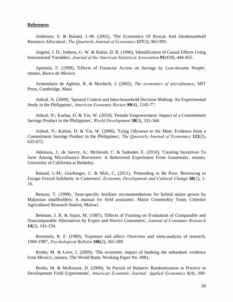
Figure 1 presents the timing of the experiment with reference to the Malawian agricultural

season. The baseline survey and interventions were administered in April and May 2009,

immediately before the 2009 harvest.

Financial Education Session

After the baseline was administered, all clubs (ordinary and commitment treatments as well

as control) attended a financial education session that reviewed basic elements of budgeting and

explained the benefits of formal savings accounts, in particular how they could be used to set

aside funds for future expenses. The full script of the financial education session can be found in

Appendix A.

The financial education session was deliberately provided to both treatment and control

groups so that treatment effects could be attributed solely to the provision of the financial

products, abstracting from the effect of financial education (for example, strategies for improved

budgeting) implicitly provided during the product offer. For this reason, we can estimate neither

11 At baseline, 89.5% and 99.9% of farmers were applying less than the recommended amount of nitrogen and

phosphorus, respectively, on their maize plots. Among farmers applying less than the recommended amount of nitrogen (phosphorus) on maize, the ratio of actual use to optimal use was 0.48 (0.14). Potassium is not recommended for maize. Nutrient recommendations for maize in central Malawi are from Benson (1999).

12 In particular, 42% of respondents were able to compute 10% of 10,000, 63% were able to divide MK 20,000 by five and only 27% could apply a yearly interest rate of 10% to an initial balance to compute the total savings balance after a year.

13 This number includes a number of “payroll” accounts opened in a previous season by OIBM and one of the tobacco buyer companies as a payment system for crop proceeds, and which do not actually allow for savings accumulation. Our baseline survey unfortunately did not properly distinguish between these two types of accounts.

7

the impact of the ordinary and commitment treatments without such financial education, nor the

impact of the financial education alone.14

Ordinary and Commitment Treatments

Farmers were randomly assigned to one of three savings treatment conditions. To minimize

cross-treatment contamination, randomization was carried out at the level of farmer clubs (of

which there were 299, described further below). The first experimental group was the control

group and only received the financial education session described above.

Implementation of the savings treatment took advantage of the existing system of depositing

crop sale proceeds into OIBM bank accounts. In the control group, the process followed the

status quo, as follows. At harvest, farmers sold their tobacco to the company at the price

prevailing on the nearest tobacco auction floor.15 The proceeds from the sale were then

electronically transferred to OIBM, which deducted the loan repayment (plus fees and

surcharges) of all borrowers in the club, and then credited the remaining balance to a club

account at OIBM. Club members authorized to access the club account (usually the chairman or

the treasurer) came to OIBM branches and withdrew the funds in cash.

Farmers in the savings treatment groups were given the same financial education session

provided to the control group, and in addition were also given account opening assistance and

offered the opportunity to have their harvest proceeds (net of loan repayment) directly deposited

into individual accounts in their names (see Figure 2 for a schematic illustration of the money

flows). After their crop was sold, farmers traveled to the closest OIBM branch to confirm that

positive proceeds net of repayment were available at the club level. Authorized members of the

clubs (often together with other club members) then filled out a sheet specifying the division of

the total amount between farmers. Depending on whether a club member had opted for the

individual accounts or not, funds were then either transferred to the individual’s account(s)

opened at the time of the intervention, prior to the harvest, or paid out in cash.

There were two savings treatment conditions. In the first, farmers were offered only an

ordinary savings account (the “ordinary” treatment). In the second, farmers were offered both an

14 Karlan et al. (2012) conduct a field experiment in Ghana where eligible individuals who already have a

savings account are allowed to open and label a second account. They find that savings in this group is 31 % larger. A subset of the individuals that opened the second account was asked to state a savings goal for this account, but they find that setting a savings goal had no impact on savings balance, suggesting that it was the opening of the second account and labeling it what was driving the results.

15 The tobacco growing regions are divided among the two tobacco buyer companies. In their coverage area each buyer company organizes farmers into clubs and provides them with basic extension services.

8

ordinary and a commitment savings account (the “commitment” treatment). Farmers who chose

to open a commitment savings account were also required to have an ordinary account where

uncommitted funds would be deposited. Farmers in the control group and the “ordinary”

treatment group who could have learned about and requested commitment accounts were not

denied those accounts, but they were not given information about or assistance in opening

them.16

An ordinary savings account is a regular OIBM savings account with an annual interest rate

of 2.5%. The commitment savings account has the same interest rate but allows farmers to

specify an amount and a “release date” when the bank would allow access to the funds.17

During the account opening process, farmers stated how much they wanted deposited in the

ordinary and commitment savings accounts after the sale of their tobacco crops. For example, if

a farmer stated that that he wanted MK 40,000 in an ordinary account and MK 25,000 in a

commitment savings account, funds would first be deposited into the ordinary account until MK

40,000 had been deposited, then into the commitment savings account for up to MK 25,000, with

any remainder being deposited back into the ordinary account.

Raffle Treatments

To study the impact of public information on savings and investment behavior, we

implemented a cross-cutting randomization of a savings-linked raffle. Participants in each of our

two savings treatments were randomly assigned to one of three raffle conditions. These raffles

provided a mechanism for revealing individual savings balances in public. We distributed tickets

for a raffle to win a bicycle, where the number of tickets each participant received was

determined by his or her savings balance as of pre-announced dates. Every MK 1,000 saved with

OIBM (in total across ordinary and commitment savings accounts) entitled a participant to one

raffle ticket. Tickets were distributed twice. The first distribution took place in early September,

and was based on savings as of August 19. The second distribution took place in November, and

was based on savings as of October 22. By varying the way in which tickets were distributed, we

sought to exogenously vary the information that club members had about each other’s savings.

16 Among farmers in the control group, nobody requested an ordinary or a commitment account during the

savings training at baseline. According to OIBM administrative records, eight farmers in the control group had commitment accounts by the end of October 2009 (opened without our assistance or encouragement), but none of these had any transactions in the accounts.

17 By design, funds in the commitment account could not be accessed before the release date. In a small number of cases OIBM staff allowed premature withdrawals of funds when clients presented evidence of emergency needs, e.g. health or funeral expenditures.

9

Because the raffle itself could provide an incentive to save or could serve as a reminder to

save (Karlan, McConnell, Mullainathan, Zinman, 2010 and Kast, Meier and Pomeranz, 2012),

one third of all clubs assigned to either ordinary or commitment savings accounts was randomly

determined to be ineligible to receive raffle tickets (and was not told about the raffle). Another

one third of clubs with savings accounts was randomly selected to have raffle tickets distributed

privately. Study participants were called to a meeting for raffle ticket distribution but were

handed their tickets out of view of other study participants. The final third of clubs with savings

accounts was randomly selected for public distribution of raffle tickets. In these clubs, each

participant’s name and the number of tickets received was announced verbally to everyone that

attended the raffle meeting.

Because of the simple formula for determining the number of tickets, farmers in clubs

where tickets were distributed publicly could easily estimate how much other members of the

club had saved. Private distribution of tickets, though, did not reveal information about

individuals’ account balances. The raffle scheme was explained to participants at the time of the

baseline survey using a simulation. Members were first given hypothetical balances, and then

given raffle tickets in a manner that corresponded to the distribution mechanism for the treatment

condition to which the club was assigned. In clubs assigned to private distribution, members

were called up one by one and given tickets in private (out of sight of other club members). In

clubs assigned to public distribution, members were called up and their number of tickets was

announced to the group.

The design of the project, therefore, includes seven treatment conditions: a pure control

condition without savings account offers or raffles; ordinary savings accounts with no raffles,

with private distribution of raffle tickets, and with public distribution of raffle tickets; and

commitment savings accounts with no raffles, with private distribution of raffle tickets, and with

public distribution of raffle tickets (see Table 2).

As mentioned, the randomization was carried out at the club level. The list of tobacco clubs

in central Malawi (all of which had existing production loans with OIBM) was provided by

OIBM in cooperation with the two tobacco buyer companies. Prior to randomization, treatment

clubs were stratified by location,18 tobacco type (burley, flue-cured or dark-fire) and week of

18 “Locations” are the tobacco buying companies’ geographically-defined administrative units within which

extension services and contract buying activities are coordinated.

10

scheduled interview. The stratification of treatment assignment resulted in 19 distinct

location/tobacco-type/week stratification cells.

The sample consists of 299 clubs with 3,150 farmers surveyed at baseline, and 298 clubs

with 2,835 farmers surveyed at endline.19 Attrition from the baseline to the endline survey was

10.0% and does not vary substantially by treatment status (as shown in Appendix Table 1).

While attrition is uncorrelated with treatment assignment for five out of the six treatment groups,

farmers in the ordinary (private raffle) treatment group have a three percentage point lower rate

of attrition from baseline to endline survey, compared to the control group, and this difference is

statistically significant at the 10% level (p-value 0.085 in the specification with full baseline

controls). Since the difference is very small, we do not view this as an important concern.

Balance of baseline characteristics across treatment conditions

To examine whether randomization across treatments achieved balance in pre-treatment

characteristics, Table 3 presents the differences in means of 17 baseline variables for the six

treatment groups vis-a-vis the control group. For statistical inference about the differences in

means we estimate a regression of each baseline variable against the two savings treatment

indicators (Commitment and Ordinary), the four respective interactions with the raffle treatment

indicators (Public or Private) and the stratification cell dummies.

With a few exceptions, baseline variables for the ordinary and commitment (without raffle)

treatment groups are well balanced with the control group. The exceptions are that individuals in

the ordinary group are more likely to be female (column 1), less likely to be married (column 2),

and less likely to be “patient now, impatient later” (column 14); and individuals in the

commitment group are more likely to be female. Overall, however, for both the ordinary and

commitment (no raffle) groups we cannot reject the null that means of all 17 baseline variables

are jointly equal to those in the control group (see p-values of F-tests at the bottom of Table 3).

The situation is similar for the coefficients on the interactions between the savings and raffle

treatments – most outcomes are balanced vis-à-vis the corresponding “no raffle” savings

treatment, with a scattering of statistically significant differences that are not too different from 19 60 clubs in two locations had to be excluded from the sample because of serious implementation

irregularities. Clubs in Kasungu Central were discovered to contain substantial numbers of “ghost” (nonexistent) club members and served as vehicles for larger landowners to fraudulently obtain very large loans from our partner institution; survey data collected for these individuals is thus likely to be fictitious. Clubs in Mndolera were excluded because of clerical and communications errors that led to ambiguity in treatment assignment. In the two locations subject to these issues, we excluded all clubs (amounting to three stratification cells) from the sample. Because entire stratification cells were excluded, inference among the remaining stratification cells yields internally valid results.

11

what would likely have arisen by chance. Again, for none of the raffle sub-treatments can we

reject the null at conventional levels that the full set of baseline variables is jointly equal to the

mean for the corresponding “no raffle” treatment.

At any rate, and to alleviate any concern that baseline imbalance may be driving our results,

we follow Bruhn and McKenzie (2009) and include the full set of baseline characteristics in

Table 3 as controls in our main regressions, in addition to the stratification cell fixed effects.20

3. Estimation strategy

A number of dependent variables are of interest, such as deposits and withdrawals prior to

the next planting season, inputs used in the next planting, crop output and sales in the next

planting, and household expenditures after the next harvest.

To estimate the impact of the treatments we estimate the following regression equation,

similar to the specification used in Table 3 when checking for balance across baseline

characteristics:

(1) Yij = δ + α1Commitmentj + α2Ordinaryj

+ α3Com_Rafj + α4Com_PubRafj

+ α5Ord_Rafj + α6Ord_PubRafj

+β’Xij + εij

Yij is the dependent variable of interest for farmer i in club j. Commitmenti is an indicator

variable for assignment to the commitment treatment and Ordinaryi is an indicator variable for

assignment to the ordinary treatment. Com_Rafj is an indicator for assignment to any raffle

treatment (either private or public) for the commitment savings treatment group, and

Com_PubRafj is an indicator for assignment to the public raffle treatment specifically. Ord_Rafj

and Ord_PubRafj are defined analogously, but for the ordinary savings treatment group. Xij is a

vector that includes stratification cell dummies and control variables measured in the baseline

survey, prior to treatment (the 17 baseline variables in Table 3) and εij is a mean-zero error.

Because the unit of randomization is the club, standard errors are clustered at this level (Moulton

1986).

Coefficients α1 and α2 measure the difference in means of the dependent variable between

the commitment treatment and the ordinary treatment, respectively (without additional raffle 20 Results turn out to be very similar when only stratification cell fixed effects are included. See Appendix

Tables 2, 3 and 4.

12

treatments) vis-à-vis the control group. The difference (α2 - α1) represents the difference in means

between the commitment treatment and the ordinary treatment (each without layered-on raffle

treatments). The coefficient α3 is the difference in means between the no-raffle commitment

treatment group and the commitment treatment combined with the private raffle treatment. The

coefficient α4 represents the difference in means between the commitment treatment with a

public raffle and the commitment treatment group with private raffle. Put differently, coefficient

α4 represents the additional impacts of making the raffle public, over and above the private raffle

treatment for the commitment savings group. Similarly, the coefficient α5 measures the

difference in means between the no-raffle ordinary treatment group and the ordinary treatment

group with private raffle. The coefficient α6 is the difference in means between the ordinary

treatment with a public raffle and the ordinary treatment group with private raffle.

Therefore, α1 + α3 is the total impact of the commitment treatment with private raffle, and α1

+ α3 + α4 is the total impact of the commitment treatment with public raffle. α2 + α5 is the total

impact of the ordinary treatment with private raffle, and α2 + α5 + α6 is the total impact of the

ordinary treatment with public raffle.

We focus on intent-to-treat (ITT) estimates because not every club member offered account

opening assistance decided to open the account. We do not report average treatment on the

treated (TOT) estimates because it is plausible that members without accounts are influenced by

the training script itself or by members who do open accounts in the same club, either of which

would violate the Stable Unit Treatment Value Assumption (SUTVA) (Angrist, Imbens and

Rubin, 1996).

4. Empirical results: impact of treatments

To understand the impacts of access to formal savings, we first study the extent to which

funds flowed into and out of the savings accounts in the pre-planting and planting periods. Then

we examine impacts on agricultural inputs, farm output, household expenditures and other

household outcomes.

A. Impacts on savings transactions (deposits and withdrawals) and savings balances

Table 4 presents regression results from estimating Equation 1. The dependent variables are

various deposit and withdrawal outcomes from administrative records of our partner institution,

OIBM. The first column presents results in which the dependent variable is an indicator variable

13

for whether any transfers were made from the club account to the farmer’s individual account

after the group loan had been repaid. This is essentially an indicator for “take-up” of the savings

treatments. Columns 2 to 7 present results for three types of savings behaviors in March to

October 2009, the “pre-planting” period: total deposits (separately for ordinary, commitment and

other accounts, as well as the sum across all accounts), total withdrawals, and net deposits into

OIBM accounts.21 This pre-planting period is when funds are accumulated from the previous

season’s harvest and when inputs are purchased for the 2009-2010 growing season.

Results from column 1 show that while none of the farmers in the control group transferred

money via direct deposit into an OIBM account (since they were not offered direct deposit nor

account opening assistance), 16% of farmers in the ordinary account, no raffle treatment did

transfer money. This percentage is somewhat larger at 21% for farmers in the commitment

savings treatment without raffle. There are no statistically significant differential effects of either

the public or private raffle on this take-up indicator. Among the individual baseline

characteristics in Table 1, we find that age, education, household size and having a prior account

with OIBM correlate positively and significantly with receiving a deposit into the ordinary

account. Interestingly, net transfers made during the year prior to the intervention are also

correlated with this take-up indicator. These correlations suggest that richer farmers are more

likely to receive a direct deposit into their ordinary accounts.

Turning to dependent variables related to deposits, both ordinary and commitment

treatments led to higher total deposits as well as higher total withdrawals during the pre-planting

period compared to the control group. Coefficients on both types of savings treatments are

statistically significantly different from zero for deposits (column 2) as well as for withdrawals

(column 3). The coefficient on the commitment (no raffle) treatment is nearly identical to the

coefficient on the ordinary (no raffle) treatment.

We note that the private raffle leads to lower deposits as well as lower withdrawals for both

types of treatments (columns 2 and 3). This result is surprising as we had expected that the

private raffle, by providing an incentive to save without direct revelation of the individual’s

savings balance, would have a positive effect, or at worst a zero effect. However, because only a

minority of participants had positive deposits at the time the raffles were conducted, individuals

who had no savings did not attend the raffle meeting. As a result, we speculate that simply

21 Net deposits are deposits minus withdrawals. For accounts opened in March or later (i.e., for all accounts

opened by our project), “net deposits” is equal to the account balance at the end of the time period (Oct 2009).

14

showing up at the meeting would have been a signal that the individual had positive savings of at

least MK1,000 (the minimum amount necessary to receive a raffle ticket).22 The coefficient on

“Ordinary x Raffle x Public” is the differential effect of the public raffle vs. the private raffle for

the ordinary treatment. In columns 2 and 3 these coefficients are about the same magnitude as

the corresponding coefficients on “Ordinary x Raffle” but of the opposite sign, and are

statistically significantly different from zero at the 10% level. These results indicate that the

negative effect of the private raffle on the ordinary treatment effect does not hold for the public

raffle. It is possible that the public treatment may have led to differentially higher savings by

fostering competition or social comparisons with others in the group, offsetting the negative

effect of the private raffle.23 The coefficients on the corresponding raffle indicators for the

commitment treatment are of similar signs, but are uniformly smaller in magnitude and are not

statistically significantly different from zero.

Overall, the private and public raffle results on deposits and withdrawals are unexpected,

and so our interpretation of the patterns is somewhat speculative. In subsequent tables nearly all

coefficients on the raffle interaction terms are not statistically significantly different from zero,

possibly due to the lack of power given that few farmers participated in the raffle.24 We therefore

limit subsequent discussion of the raffle results in this paper.

To further explore the impact on deposits, we separately examine impacts on three different

components of deposits in the pre-planting period: deposits into ordinary accounts (column 4),

commitment accounts (column 5), and other accounts not set up by the project (column 6). It is

clear that most of pre-planting deposits go into ordinary accounts, even among farmers in the

commitment (no raffle) treatment. The relative sizes of the coefficients on the commitment (no

raffle) treatment in columns 4 and 5 indicate that 89% of pre-planting deposits (MK 19,464.30

22 There are other possible explanations for the negative effect of the private raffle on savings. Study

participants may have overestimated the expected value of their raffle tickets, and saved less as a result. In addition, individuals may have planned to deposit funds at some later date (because the raffle tickets would be awarded based on balances as of specific dates in August and October), but may have ended up depleting their cash stocks in the interim or otherwise failing to make those later deposits.

23 At the same time, the private raffle treatment may have “primed” individuals to worry about demands from others who might learn they were saving, while the public treatment may have primed individuals to raise their social status by saving more than others. Key references in the psychology literature on priming include Bornstein (1989), Bettman and Sujan (1987), and Zajonc (1968), who document situations where decisions can be influenced by highly local or transitory influences, such as the introduction of certain concepts.

24 One could also argue that the null effects of the raffle on subsequent outcomes are due to the irrelevance of the raffle because other club members are not part of one’s risk sharing network or the irrelevance of the public vs private treatment because club members are familiar with each other balances as they jointly filled out the sheet that specified how total club sales had to be divided among members.

15

out of total deposits of MK 21,861.22) by farmers in the commitment (no raffle) treatment

actually went into the ordinary savings accounts, rather than the commitment accounts.

This finding that most of the savings in the commitment (no raffle) treatment were actually

deposited in ordinary accounts is one of the key results of the paper, and helps rule out an

important potential channel through which the commitment treatment may have had its effects.

Because the amount deposited in the commitment account was several times smaller than the

increase of input usage on average (to be documented in the next section), it cannot be the case

that the commitment account helped farmers deal with their self-control problem by literally

“tying their hands”.

In column 7 we turn to net deposits during the pre-planting period. The commitment savings

(no raffle) treatment led to a small and statistically significant increase in net deposits, while the

effect of the ordinary (no raffle) treatment was not statistically different from zero. The

difference in coefficients between ordinary and commitment treatments is not statistically

significantly different from zero, however.

The “growing” period, from November 2009 to April 2010, is conveniently divided into the

“planting” period from November to December 2009, when land is prepared, seeds are sown and

fertilizer is applied, and January through April 2010, which is the lean or “hungry” season when

households may have depleted stocks of maize from the previous season’s harvest and have not

yet harvested crops or received payments for the 2010 harvest. In column 8 of Table 4, we

examine net deposits during the first two months of the growing season, November and

December 2009. The commitment (no raffle) treatment, on net, led to higher withdrawals as did

the ordinary (no raffle) treatment. The coefficients are small in magnitude, however, indicating

impacts on net withdrawals of around MK1,000 for both treatments during this time period.

In column 9, the dependent variable is net deposits in the January to April 2010 lean or

“hungry” season; coefficients on the commitment and ordinary (no raffle) treatments are small

and not statistically significantly different from zero. Neither treatment appears to have led to

more access to saved resources during the 2010 lean season.

Time patterns of deposits and withdrawals

Table 4 documents that both deposits into and withdrawals from OIBM accounts in the 2009

pre-planting period were substantial for both the commitment and ordinary treatments. An open

question is whether most funds remained deposited in the accounts until the planting period. As

it turns out, most funds were withdrawn not long after being deposited. Figure 3 presents average

deposits into and withdrawals from ordinary and other (non-commitment) accounts, by month,

16

from March 2009 to April 2010.25 The sample in Figure 3.a includes all individuals in a

commitment treatment (whether no-raffle or one of the raffle treatments), while the samples for

Figure 3.b include all individuals in an ordinary treatment (again with or without raffle). For

comparison, the sample used in Figure 3.c includes all individuals in the control group.

The figures indicate that peak deposits occurred in June, July, and August 2009, coinciding

with the peak tobacco sales months. Average deposits in every month for individuals in both the

commitment and ordinary treatments are quite similar in magnitude to average withdrawals,

indicating that the majority of deposited funds were withdrawn soon thereafter. As a result,

savings balances during the pre-planting period were much lower than accumulated deposited

amounts, explaining why most farmers did not participate in the raffle.26

One likely reason why funds in the ordinary accounts were withdrawn at once soon after

they had been deposited has to do with transactions costs. Farmers lived on average 20

kilometers away from the bank branch and would typically travel by foot, bus, or bicycle.27 In

addition to the commuting time, farmers report a median waiting time at the branch to withdraw

money of one hour.

In contrast to the time pattern of the ordinary accounts, funds into commitment accounts do

stay deposited for longer periods of time as expected. Figure 4 displays average deposits into and

withdrawals from commitment accounts, by month, for all individuals in a commitment

treatment (with or without raffle). For deposits, the peak months are June, July, and August,

coinciding with the peak deposit months for the ordinary accounts. But withdrawals from the

commitment accounts are delayed substantially, occurring in October, November, and

December, coinciding with the key months when agricultural inputs must be purchased and

applied on fields.

This time pattern of withdrawals from commitment accounts is consistent with the release

dates chosen by users of commitment accounts. Figure 5 presents the histogram of commitment

account release dates (when commitment account funds would be “unlocked” and funds made

available to farmers) that farmers chose during account opening. About 60% of farmers chose

release dates in the months of October to December while others chose to have access to the

funds in January and February, during the lean or “hungry” season.

25 The data presented are the sum of the dependent variables in columns 4 and 6 of Table 4. 26 The pattern is similar for individuals in the control group, but levels are much lower owing to the fact that

direct deposit from the tobacco auction floor into farmer accounts was not enabled for that group. 27 The median round-trip bus fare is MK 400 for a two hour ride one way.

17

B. Inputs, crop sales, and expenditures

We now turn to impacts of the treatments on land cultivated, inputs, crop output, and

household expenditures in Table 5. Across the six dependent variables the coefficient on the

commitment (no raffle) treatment is large, positive, and statistically significant in five out of six

columns (the exception is column 5 for farm profits, where the coefficient is marginally

significant). In comparison, the coefficients on the ordinary savings (no raffle) indicator are all

smaller in magnitude and none are statistically significantly different from zero at conventional

levels. Furthermore, the private raffle treatment never leads to a statistically significantly

different effect vis-à-vis the corresponding no-raffle treatment. Similarly, in none of the

regressions does the public raffle have effects that are statistically significantly different from the

private raffle.28

The first two columns of the table reveal that the commitment (no raffle) treatment had a

large positive and statistically significant effect on both land under cultivation and the total value

of inputs used (which include seed, fertilizer, pesticides, hired labor, transport and firewood for

curing) in the late-2009 planting.29 Farmers in the commitment group cultivated on average 0.42

more acres of land than the control group (which had 4.28 acres of land under cultivation). The

commitment coefficient is statistically significantly different (p-value 0.057) from the ordinary

coefficient of 0.05 (which in turn is not statistically significantly different from zero). Compared

to MK 60,372 in inputs used by control group farmers on average, commitment treatment

farmers used MK16,534 (or 27.4%) more. By contrast, while the coefficient on the ordinary (no

raffle) treatment is also positive, it is only about half the magnitude of the commitment (no

raffle) treatment coefficient and it is not statistically significantly different from zero. The

difference in the coefficients on the two treatments in column 2, however, is not statistically

different from zero at conventional levels.

It is noteworthy that the impact on input use is substantially larger than total savings

balances (or net deposits) at the end of October 2009, immediately prior to the typical start of the

planting season (column 7 of Table 4). Examination of the timing of withdrawals in Figure 3.b

28 The public raffle treatment in the ordinary treatment group is significant different than the control group for

most variables but as we can see from Table 3, this group is also the one that suffers from most imbalance. 29 We note that we report the cash value of inputs at baseline instead of the more comprehensive measure of

total value of inputs, which is only available at follow-up. We find similar results when we use the cash value of inputs computed at follow-up (results not shown).

18

helps shed light on when funds were likely to have been accessed for input purchases. Most

funds used to purchase inputs must have come from withdrawals before the end of October:

column 3 of Table 4 indicates that the commitment (no raffle) treatment led to total withdrawals

in the period leading up to and including October amounting to more than MK 20,000, which

exceeds the impact of the commitment (no raffle) treatment on inputs used. This time pattern

suggests that farmers withdrew funds prior to the planting season, either accumulating funds held

outside of the bank (e.g., stored at home) for later input purchases, or purchasing inputs in

advance of the planting season.30

The increase in input use due to the commitment (no raffle) treatment is 8.3 times the impact

on deposits in commitment accounts in the pre-planting period (MK 16,534 from column 2 of

Table 5 divided by MK 1,994 from column 5 of Table 4), but is well within the total amount of

deposits into ordinary and commitment savings accounts (MK 21,861 from column 2 of Table

4).31 The bulk of funds used to purchase inputs, therefore, must have come from ordinary rather

than commitment savings, and thus were available to farmers during the pre-planting period,

instead of physically being locked away at the bank. This result is inconsistent with the

hypothesis that the commitment accounts helped to solve farmers’ self-control problems by

keeping them from accessing the funds prior to the planting season.

The fact that such a large proportion of observed deposits at OIBM was allocated towards

input purchases in the commitment treatment group suggests that the funds were deposited in

accounts with the expectation at the outset that they would be used for input purchases. It should

be noted that revenues from tobacco account for only half of all household income, and so

farmers have other sources of funds (incompletely observed by us) that are used to pay for other

household expenditures.

Columns 3 and 4 indicate that the larger input use caused by the commitment treatment

resulted in higher proceeds from the sale of crops as well as total crop output in the 2010

harvest.32 Both coefficients on the commitment (no raffle) treatment in these regressions are

large in magnitude and statistically significantly different from zero at the 5% level. The increase

30 Duflo, Kremer, and Robinson (2011) show that interventions encouraging advance fertilizer purchases raise

fertilizer use in western Kenya. 31 As we shall see in the next section, the increase in input use does not appear to be driven by higher

borrowing. 32 Since the baseline was conducted right before the harvest, we only collected the proceeds from crop sales for

the 2008 season. The value of crop output (sold and unsold) is only available for the follow-up survey after the harvest of 2010.

19

in crop sales (MK 22,962.78) comes exclusively from tobacco sales rather than maize sales since

the latter do increase significantly. The increase in total value of crop output (MK 33,968)

amounts to 21.8% of mean crop value in the control group. The coefficient on the ordinary (no

raffle) treatment in this column is also positive but its magnitude is much smaller than the

coefficient on the commitment treatment, and it is not statistically significantly different from

zero. The difference between the ordinary (no raffle) and commitment (no raffle) coefficients in

this column is statistically different from zero at the 10% level (p-value 0.081).

Column 5 shows the impact of the treatments on farm profits, defined as the difference

between the total value of crop output (dependent variable of column 4) and the total value of

inputs used (dependent variable of column 2).33 The coefficient on the commitment treatment is

large in economic terms and marginally statistically significant. The coefficient for the ordinary

account is small and not statistically significant, and the difference vis-a-vis the commitment

account is marginally significant (p-value 0.142).

Column 6 examines the impact of the treatments on total household expenditures in the

endline (post-harvest) survey (fielded in July to September 2010). The commitment (no raffle)

treatment coefficient is positive and statistically significantly different from zero at the 5% level,

while the coefficient on the ordinary (no raffle) treatment is substantially smaller and not

statistically significantly different from zero. The commitment (no raffle) treatment effect

represents a 17.4% increase total expenditures over the last 30 days compared to the control

group. 34

In order to examine further whether the commitment accounts treatment had a differential

impact vis-a-vis the ordinary accounts across the set of outcomes in Table 5, we follow Kling,

Liebman and Katz (2007) and present p-values of three F-tests at the bottom of Table 5 that are

based on seemingly unrelated regression (SUR) estimation. We simultaneously estimate equation

1 with the dependent variables of columns 1, 2, 4 and 6.35 The test that the coefficient on the

33 The coefficients of column 5 are not exactly (though nearly) numerically identical to the difference between the coefficients from column 4 and 2 since survey variables are winsorized (see Appendix B for details).

34 We also check whether the results are driven by those that take-up the accounts and receive a deposit into their accounts among all those offered the accounts. In particular, we use specification (1) and include interactions of treatment dummies with an indicator of take-up (the dependent variable in column 1, Table 4). As expected, we find that the interaction of commitment (no raffle) dummy with take-up is positive and significant in three out of the five variables of Table 5 (results not shown). This provides suggestive evidence that the results are driven by the compliers.

35 We restrict attention to just the regressions for the four outcomes in columns 1, 2, 4, and 6 of Table 5 because farm profit in column 5 is simply the difference between the dependent variables in columns 2 and 4 and

20

commitment (no raffle) treatment is jointly equal to zero across the four regressions is rejected at

conventional levels of statistical significance (p-value 0.042). In contrast, we cannot reject that

the coefficient for the ordinary (no raffle) treatment is jointly equal to zero across the four

regressions (p-value 0.694). We also fail to reject however that the coefficients on the ordinary

(no raffle) treatment equals the coefficients on the commitment (no raffle) treatment across the

regressions of columns 1, 2, 4, and 6 (p-value 0.254).

C. Other outcomes and mechanisms

Table 6 presents regression results on the impacts of the treatments on household size,

transfers to and from the social network, loans taken out to finance the agricultural investment

and demand for fixed deposit accounts, measured at the endline survey.

Column 1 shows that the intervention had no effect on household size. This implies that the

impacts presented in Table 5 are driven by changes in agricultural decisions and outcomes rather

than changes in household composition.

Transfers sent and received are of particular interest because a potential channel of the

observed impact of the commitment treatment may be an increased ability to resist demands

from the social network. Although net balances in the commitment accounts were small, the

existence of the account may have provided an excuse to turn down requests for assistance from

the social network by claiming that savings were inaccessible. Even though most of farmers’

funds were in ordinary accounts, this could have been a credible claim because the division of an

individual’s funds between ordinary and commitment accounts was not directly observable to

others.36

In columns 2, 3 and 4 of Table 6 we examine the sums of transfers made, transfers received

and net transfers over the last twelve months.37 We find no evidence of reduced net transfers for

the commitment (no raffle) treatment. If anything, there is a small positive, effect on net transfers

made (column 4).38 This result fails to support the hypothesis that the channel through which

commitment accounts led to increased input use was via an increased ability to resist sharing

cannot therefore be separately determined. Similarly, the proceeds from crop sales are included in the value of crop sold in column 4.

36 Even the public raffle treatments only provided a signal of an individual’s total balances at OIBM, not how those savings were split between ordinary and commitment accounts.

37 The coefficients of column 4 are not exactly (though nearly) numerically identical to the difference between the coefficients from column 3 and 2 since survey variables are winsorized (see Appendix B for details).

38 In a very different context, this result is similar to that of Chandrasekhar et al. (2012), who show in a lab-in-the-field experiment among Indian villagers that savings access does not crowd out transfers to others.

21

with one’s social network.

We note that the transfers studied in columns 2, 3 and 4 refer to inter-household transfers,

and do not capture any changes in intra-household transfers. It is possible that the commitment

treatment effect operated at least in part by reducing transfers by study participants to spouses

and other individuals within the same household. Alternatively, the null effect on total transfers

(column 2) could be the result of lower transfers made during the pre-planting season while the

commitment account was active (and thus the excuse that funds were locked up valid) but higher

after the harvest given that agricultural production had been larger. Similarly, farmers in the

ordinary treatment may have spent savings quickly to avoid the pressure to share them with

others, leading to no differences in transfers made. Unfortunately, we lack the data needed to test

these hypotheses.

Column 5 examines the largest source of borrowing for agricultural investment in inputs,

namely loans provided by a lender to the tobacco club.39 After all, the increase in total value of

inputs for the commitment treatment group could be driven by a higher loan size and not by the

increased ability to keep the funds until planting. Column 5 shows that this is not the case. The

commitment (no raffle) and ordinary (no raffle) treatment groups report loan amounts from the

tobacco club that are similar to those in the control group.40

Finally, we present data on subsequent opening of fixed deposit accounts (column 5) at the

time of the endline survey. Fixed deposit accounts in Malawi typically have a duration of three

or six months. The client makes an initial one-time deposit of pre-specified amounts, typically in

multiples of MK10,000. During the three- or six-month duration the client cannot make a

withdrawal from the fixed deposit account and also cannot increase the savings balance.

Interestingly, we find that ownership of fixed deposit accounts is six percentage points

higher and significant at the 1% level in the commitment (no raffle) group, and three percentage

points higher in the ordinary (no raffle) group (significant at the 5% level) compared to the

control group (this difference in treatment effects across the ordinary and commitment treatments

is not significantly different from zero at conventional levels).

The positive impact on subsequent ownership of fixed deposit accounts suggests that the

commitment treatment caused farmers to raise their perceived value of commitment features in

39 Loans from informal lenders and friends and family account for a small fraction of total borrowings. At any

rate, total credit instead of tobacco credit yield very similar results. 40 Similarly, we find no difference across treatment and control groups in the probability of accessing a loan

(results not shown).

22

formal savings accounts. This reinforces the interpretation of our results as causal effects of the

commitment treatment rather than spurious correlations, insofar as higher demand for fixed

deposit accounts reflects farmers’ own recognition that such accounts have some benefits.

However, this evidence does not help differentiate between self- and other-control problems as

sources of demand for commitment, and also does not rule out the possibility that other

psychological channels may be at work.

5. Conclusion

We find that offering commitment savings accounts to smallholder cash crop farmers in

Malawi has substantial impacts on formal bank deposits and withdrawals prior to the next

planting season, agricultural inputs applied in the next planting season, crop sales at the next

harvest, and total household expenditures after the next harvest. While offers of “ordinary” bank

accounts also lead to deposits of similar magnitudes, effects on agricultural input use and other

subsequent outcomes are smaller and statistically insignificant.

Given the large impacts of the commitment treatment, it is important to ask why the

treatment had such substantial effects, while the ordinary treatment did not. Several possible

mechanisms exist. First, the commitment account may have helped farmers solve their self-

control problems, giving them the discipline to maintain their balances until the next planting

season when they could be used for agricultural inputs. Alternatively, the commitment accounts

may have helped farmers to refrain from sharing with others in their social network. An

additional possibility is that the commitment accounts may have increased later input use via

some other psychological channel.

We provide evidence against the hypothesis that the commitment treatment helped via

solving farmers’ self-control problems. The actual amounts saved in the commitment accounts

were very low (about an order of magnitude lower than the observed increase in inputs), with

ordinary accounts receiving the vast majority of deposits. The observed increase in input use due

to the commitment treatment plausibly could have been funded out of deposits into ordinary

accounts, but is much too large to have been funded purely out of deposits in commitment

accounts. This rules out that the impacts of the commitment treatment were due to literally “tying

the hands” of treated farmers by preventing them from spending their profits earlier in the year.

We also find no evidence that the commitment treatment helped solve “other-control”

problems (demands for sharing of resources with one’s social network). The commitment

23

treatment did not reduce net transfers to other households (and in fact had a small positive impact

on such transfers). Relatedly, a sub-experiment testing the impact of making one’s account

balances public to others also did not find that public revelation of balances reduced savings

deposits. That said, the case against the importance of other-control in this context is not

conclusive. The transfer variables we examined refer to inter-household transfers, and do not

capture any changes in intra-household transfers. It remains possible that the commitment

treatment effect operated at least in part by reducing transfers by study participants to spouses

and other individuals within the same household.

Another caveat regarding the other-control results is that though we do not find evidence that

commitment savings accounts reduced transfers to other members of the social network, the

accounts may have helped farmers increase their input use by mitigating another possible

consequence of social pressure to share. Individuals who know they will be subject to demands

from others in their social network can prevent others from claiming their money by spending it

preemptively. Rapidly consuming income makes it unavailable to others; it is consistent with

signaling a high marginal utility of consumption in a model where income is taxed and

redistributed from those with low marginal utility of consumption to high marginal utility of

consumption. Goldberg (2011) found support for such a model in an experiment that

demonstrated that Malawian cash crop farmers who received money in public settings spent

significantly more of that money immediately than farmers who received money in private

settings. In this project, we do not have the high-frequency consumption data necessary to test

whether farmers with commitment savings accounts were less likely to engage in hasty

consumption than farmers without such accounts. However, a reduction in sub-optimally timed

consumption is a channel through which offers of commitment accounts could have led to

increased use of inputs and improvements in output, profits, and household expenditures. In

future related work we will examine whether commitment savings offers affect such

“anticipatory consumption” by examining the timing and composition of expenditures in the

post-harvest months. Future research is thus still needed to shed light on the importance other-

control problems as a potential hindrance to savings.

We can provide no empirical evidence as to whether mental accounting or some other

psychological phenomenon may be behind the impact of the commitment treatment.

Investigating this possible channel for the effects of the commitment treatment is also an

important area for future research.

24

While the well-being of farmers offered commitment accounts is likely to have improved,

we do not shed light directly on impacts on others in the community. An initial worry was that

the commitment accounts led farmers to make fewer transfers to others in the community in the

context of informal insurance arrangements (for example, to help others cope with shocks). As it

turns out, we do not find any negative impacts of the commitment treatment on net transfers to

other households. That said, reduced “anticipatory consumption” in the months immediately

after the intervention may have had negative impacts via reduced demand for goods and services

produced by others in the community. We view investigation of longer-term impacts on study

participants and on others in the community as an important area for future research.

25

References

Anderson, S. & Baland, J.-M. (2002), 'The Economics Of Roscas And Intrahousehold Resource Allocation', The Quarterly Journal of Economics 117(3), 963-995.

Angrist, J. D.; Imbens, G. W. & Rubin, D. B. (1996), 'Identification of Causal Effects Using

Instrumental Variables', Journal of the American Statistical Association 91(434), 444-455. Aportela, F. (1999), 'Effects of Financial Access on Savings by Low-Income People',

mimeo, Banco de Mexico. Armendariz de Aghion, B. & Morduch, J. (2005), The economics of microfinance, MIT

Press, Cambridge, Mass. Ashraf, N. (2009), 'Spousal Control and Intra-household Decision Making: An Experimental

Study in the Philippines', American Economic Review 99(4), 1245-77. Ashraf, N.; Karlan, D. & Yin, W. (2010), 'Female Empowerment: Impact of a Commitment

Savings Product in the Philippines', World Development 38(3), 333-344. Ashraf, N.; Karlan, D. & Yin, W. (2006), 'Tying Odysseus to the Mast: Evidence from a

Commitment Savings Product in the Philippines', The Quarterly Journal of Economics 121(2), 635-672.

Atkinson, J.; de Janvry, A.; McIntosh, C. & Sadoulet, E. (2010), 'Creating Incentives To

Save Among Microfinance Borrowers: A Behavioral Experiment From Guatemala', mimeo, University of California at Berkeley.

Baland, J.-M.; Guirkinger, C. & Mali, C. (2011), 'Pretending to Be Poor: Borrowing to

Escape Forced Solidarity in Cameroon', Economic Development and Cultural Change 60(1), 1-16.

Benson, T. (1999), 'Area-specific fertilizer recommendations for hybrid maize grown by

Malawian smallholders: A manual for field assistants', Maize Commodity Team, Chitedze Agricultural Research Station, Malawi.

Bettman, J. R. & Sujan, M. (1987), 'Effects of Framing on Evaluation of Comparable and

Noncomparable Alternatives by Expert and Novice Consumers', Journal of Consumer Research 14(2), 141-154.

Bornstein, R. F. (1989), 'Exposure and affect: Overview and meta-analysis of research,

1968-1987', Psychological Bulletin 106(2), 265-289. Bruhn, M. & Love, I. (2009), 'The economic impact of banking the unbanked: evidence

from Mexico', mimeo, The World Bank, Working Paper No. 4981. Bruhn, M. & McKenzie, D. (2009), 'In Pursuit of Balance: Randomization in Practice in

Development Field Experiments', American Economic Journal: Applied Economics 1(4), 200-

26

232. Burgess, R. & Pande, R. (2005), 'Do Rural Banks Matter? Evidence from the Indian Social

Banking Experiment', The American Economic Review 95(3), 780-795. Chandrasekhar, A.; Kinnan, C. & Larreguy, H. (2012), 'Informal Insurance, Social

Networks, and Savings Access: Evidence from a Lab Experiment in the Field', mimeo, Northwestern University.

Cole, S.; Sampson, T & Zia, B. (2011), ‘Prices or Knowledge? What Drives Demand for

Financial Services in Emerging Markets?’ Journal of Finance, 66(6), 1933-1967. Collins, D.; Morduch, J.; Rutherford, S. & Ruthven, O. (2009), Portfolios of the Poor: How

the World's Poor Live on $2 a Day, Princeton University Press. Daley-Harris, S. (2009), 'State of the Microcredit Summit Campaign Report 2009',

Microcredit Summit Campaign, Washington, DC. Deaton, A. (1990), ‘Saving in Developing Countries: Theory and Review’, Proceedings of

the World Bank Annual Conference on Development Economics 1989. Supplement to The World Bank Economic Review and the World Research Observer, pp. 61-96.

Duflo, E.; Kremer, M. & Robinson, J. (2008), 'How High Are Rates of Return to Fertilizer?

Evidence from Field Experiments in Kenya', The American Economic Review Papers and Proceedings, 98(2), 482-488.

Duflo, E.; Kremer, M. & Robinson, J. (2011), 'Nudging Farmers to Use Fertilizer: Theory

and Experimental Evidence from Kenya', American Economic Review 101(6), 2350-90. Dupas, P. & Robinson, J. (2012), 'Savings Constraints and Microenterprise Development:

Evidence from a Field Experiment in Kenya', mimeo, UCLA. Dupas, P. & Robinson, J. (2012), 'Why Don’t the Poor Save More? Evidence from Health

Savings Experiments in Kenya', mimeo, Stanford University. Fafchamps, M.; McKenzie, D.; Quinn, S. R. & Woodruff, C. (2011), 'When is capital

enough to get female microenterprises growing? Evidence from a randomized experiment in Ghana', NBER Working Paper No. 17207.

Feldman, J. M. & Lynch, J. G. (1988), 'Self-generated validity and other effects of

measurement on belief, attitude, intention, and behavior', Journal of Applied Psychology 73(3), 421-435.

Flory, J. A. (2011), 'Micro-Savings & Informal Insurance in Villages: How Financial

Deepening Affects Safety Nets of the Poor - A Natural Field Experiment', Becker Friedman Institute for Research in Economics, University of Chicago, Working Paper No. 2011-008.

Giné, X.; Goldberg, J. & Yang, D. (2012), 'Credit Market Consequences of Improved

Personal Identification: Field Experimental Evidence from Malawi', American Economic Review

27

102(6): 2923-2954. Goldberg, J. (2011), 'The Lesser of Two Evils: The Roles of Self-Interest and Impatience in

Consumption Decisions', mimeo, University of Maryland. Hertzberg, A. (2010), 'Exponential Individuals, Hyperbolic Households', mimeo, Columbia

University. Hoff, Karla and Arijit Sen (2006), “The Kin System as a Poverty Trap?” in Poverty Traps

Bowles, Samuel, Steven Durlauf and Karla Hoff (eds), Princeton University Press, pp. 95-115. Jakiela, P. & Ozier, O. (2011), 'Does Africa Need a Rotten Kin Theorem? Experimental

Evidence from Village Economies', mimeo, University of Maryland. Kahneman, D. & Tversky, A. (1979), 'Prospect Theory: An Analysis of Decision under

Risk', Econometrica 47(2), 263-91. Karlan, D.; McConnell, M.; Mullainathan, S. & Zinman, J. (2010), 'Getting to the Top of

Mind: How Reminders Increase Saving', NBER, Working Paper No. 16205. Kast, F.; Meier, S. & Pomeranz, D. (2012), 'Under-Savers Anonymous: Evidence on Self-

Help Groups and Peer Pressure as a Savings Commitment Device', Institute for the Study of Labor (IZA), Working Paper No. 6311.

Kling, J. R.; Liebman, J. B. & Katz, L. F. (2007), 'Experimental Analysis of Neighborhood

Effects', Econometrica 75(1), 83-119. Ligon, E.; Thomas, J. P. & Worrall, T. (2002), 'Informal Insurance Arrangements with

Limited Commitment: Theory and Evidence from Village Economies', The Review of Economic Studies 69(1), 209-244.

Maranz, D. E. (2001), African Friends and Money Matters: Observations from Africa

(Publications in Ethnography, Vol. 37), SIL International. de Mel, S.; McKenzie, D. & Woodruff, C. (2008), 'Returns to Capital in Microenterprises:

Evidence from a Field Experiment', The Quarterly Journal of Economics 123(4), 1329-1372. Morduch, J. (1999), 'The Microfinance Promise', Journal of Economic Literature 37(4),

1569-1614. Moulton, B. R. (1986), 'Random group effects and the precision of regression estimates',

Journal of Econometrics, 32(3), 385-397. Pearce, B., Denton, P., Schwab, G., Seebold, K. & Pearce, B., eds., (2011), 2011-2012

Kentucky & Tennessee Tobacco Production Guide, University of Tennessee and University of Kentucky, chapter Field Selection, Tillage, and Fertilization, pp. 24-29.

Platteau, J.-P. (2000), Institutions, Social Norms and Economic Development (Fundamentals

of Development Economics), Routledge.

28

Prina, S. (2011), “Do Basic Savings Accounts Help the Poor to Save? Evidence from a Field

Experiment in Nepal,” mimeo, Case Western Reserve University. Robinson, M. (2001), The Microfinance Revolution: Sustainable Finance for the Poor,

World Bank Publications. Rutherford, S. (2000), The poor and their money, Oxford University Press, New Delhi;

Oxford. Schaner, S. (2012), 'Intrahousehold Preference Heterogeneity, Commitment, and Strategic

Savings', mimeo, Dartmouth College. Thaler, R. H. (1990), 'Saving, Fungibility, and Mental Accounts', Journal of Economic

Perspectives 4(1), 193-205. Webb, T. L. & Sheeran, P. (2006), 'Does changing behavioral intentions engender behavior

change? A meta-analysis of the experimental evidence', Psychological Bulletin 132(2), 249-268. World, B. (2008), 'World Development Report: Agriculture for Development', World Bank,

mimeo, World Bank, Washington D.C. Zajonc, R. B. (1968), 'Attidunial Effects of Mere Exposure', Journal of Personality and

Social Psychology 9(2, Pt.2), 1-27. Zwane, A. P.; Zinman, J.; Van Dusen, E.; Pariente, W.; Null, C.; Miguel, E.; Kremer, M.;

Karlan, D. S.; Hornbeck, R.; Giné, X.; Duflo, E.; Devoto, F.; Crepon, B. & Banerjee, A. (2011), “Being surveyed can change later behavior and related parameter estimates,” Proceedings of the National Academy of Sciences 108(5), 1821-1826.

29

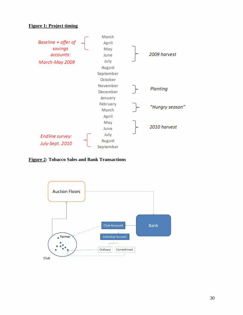
Figure 1: Project timing

Figure 2: Tobacco Sales and Bank Transactions

30

31

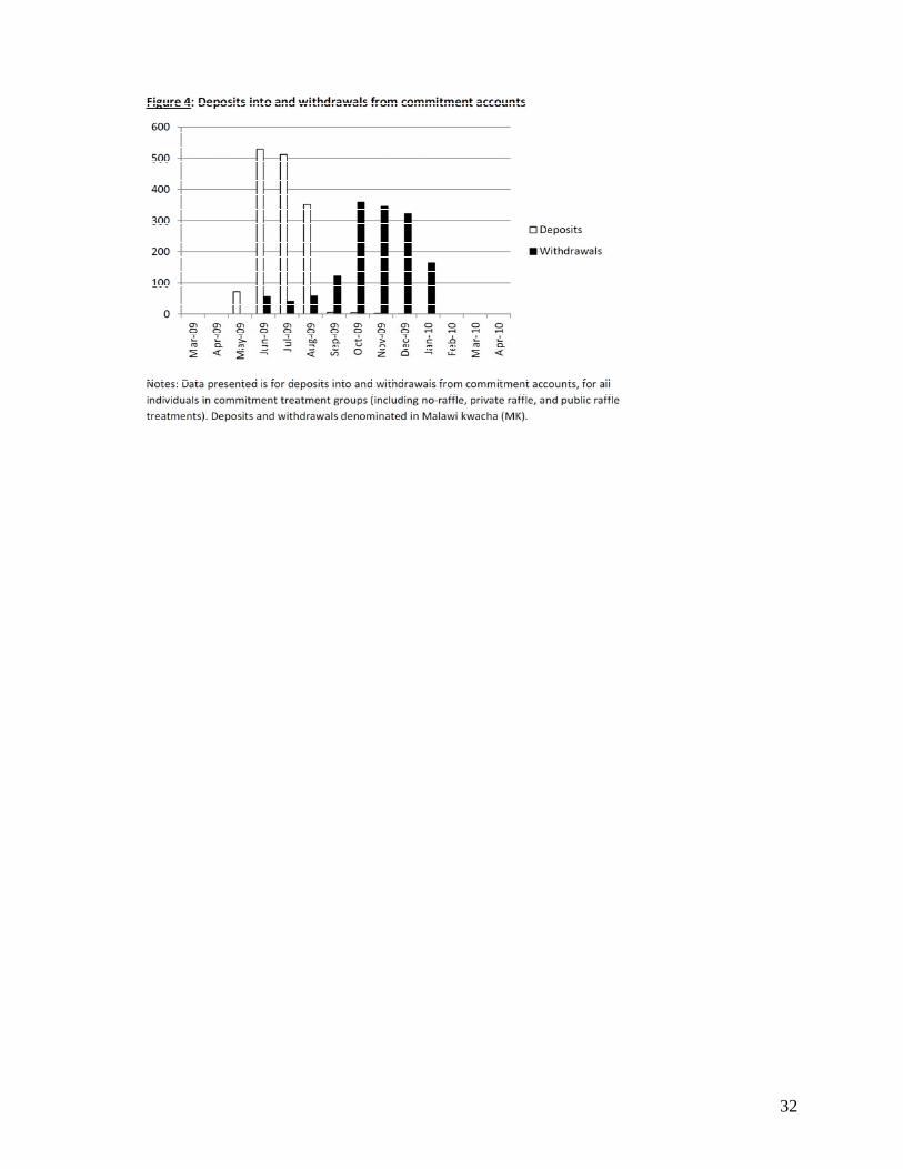
32

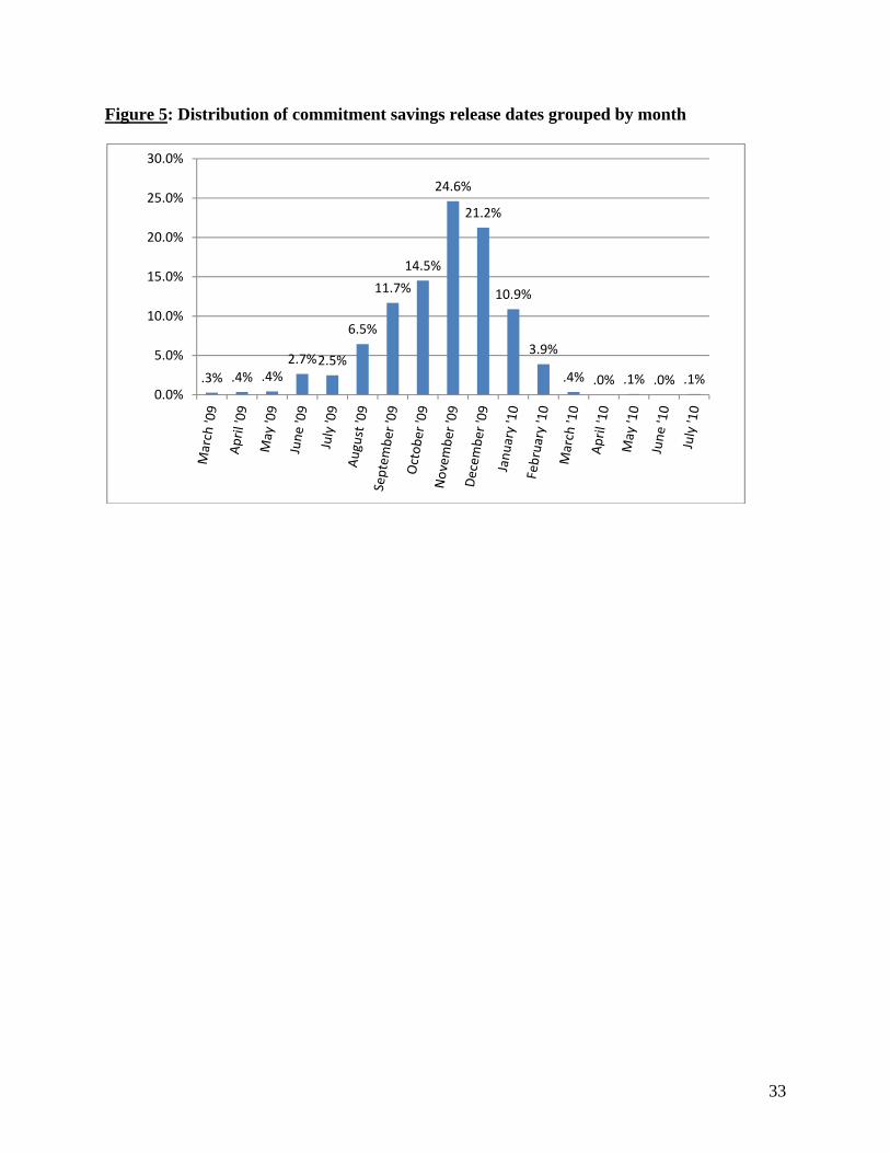
Figure 5: Distribution of commitment savings release dates grouped by month

.3% .4% .4%2.7%2.5%

6.5%

11.7%

14.5%

24.6%

21.2%

10.9%

3.9%

.4% .0% .1% .0% .1%0.0%

5.0%

10.0%

15.0%

20.0%

25.0%

30.0%

33

Appendix A: Account details and full text of training script

Savings account details In this experiment we offered farmers training and account opening assistance for two types

of accounts depending on the treatment status (control, ordinary savings or commitment savings). The “ordinary” account referred to in the main text is OIBM’s Kasupe account. Kasupe accounts had an account opening of MK500, no monthly fee, three free withdrawals transactions via ATM per month, and a MK25 fee per ATM withdrawal thereafter (all withdrawals at the teller were free). The minimum balance for Kasupe accounts was MK1,000 and there was an account closing fee of MK1,000. Kasupe accounts paid an interest rate of 2.5% p.a. with interest accruing quarterly. Deposit transactions into Kasupe accounts were free.

Farmers were given the option to have their proceeds directly deposited into an existing account if they already had a savings account with OIBM. Another type of savings account not actively marketed in this experiment but part of OIBM’s product portfolio was standard savings accounts with the following fee structure: an opening fee of MK500; a monthly fee of MK75; no withdrawal fees; minimum balance of MK1,000; a closing fee of MK1,000; an interest rate of 6.5% p.a. with quarterly accrual. This less common account type is included in the category “ordinary” accounts together with Kasupe accounts.

The “commitment” account referred to in the main text was an account newly developed for the project called “SavePlan.” SavePlan accounts paid the same interest rate as Kasupe accounts, but had no minimum balance requirement. SavePlan accounts also had no account opening or closing fees. Deposit transactions into SavePlan accounts were free. The only withdrawals permitted for SavePlan accounts were transfers to ordinary (Kasupe or other) savings accounts, for which no fee was charged.

Scripts for savings training, account offers, and raffle training (Scripts were administered in club meeting immediately following administration of baseline

survey. Malawian research project staff played the roles of Persons 1 and 2.) Section 1: Savings Accounts (All Clubs) Person 1: Saving money in an individual bank account is a very smart way to protect your money and

improve your wellbeing. As you know, OIBM has Kasupe accounts that are easy and affordable to use. Person 2: But I already have a savings account with my club. What is better about this Kasupe account? First ask the group to list things that are good about the Kasupe account. When the group has come up with

several suggestions, move on to the next line: Person 1: The Kasupe account is yours alone. You don’t share it with the rest of your club members. You are

the only one who can take money out of the account and the only one who knows how much money you have saved in the account.

Person 2: What are the details of the account? How much does it cost, and what is the interest? Person 1: MK 500 for smartcard, MK 500 for initial deposit, no monthly charge, MK 25 transaction charge

(ATM fee, withdrawal fee). Person 2: But I can just keep money at home. What are some of the benefits of saving my money in a Kasupe

account instead of at home?

34

Let the group make suggestions. After several things have been suggested, agree with the group and then move on to the next line.

Person 1: Money is safer in a bank account than at home. If you keep your money at home, it could be stolen

or lost in a fire. If you keep it at the bank, it is protected. Also, if you keep money at home, you may feel obligated to give money to your family or friends if they ask for it. If your money is in the bank, you can say that you don’t have any money to give.

Person 2: That is interesting, but I think my money is safe at home. Ask the group: “Do you think money is safe at home?” Let the group come up with answers, then move on. Person 1: There are other reasons to keep money in the bank, too. Keeping money in a bank account can help

you save for the future. If you have money at home, it is easy to be tempted to spend it on food or drinks or household items. If you have money in the bank, you will think twice about taking it out to spend. Instead, you can leave it in the bank to save for important purchases like school fees or buying fertilizer or accumulating the deposit for a new loan. Also, you can be sure to put away money in case you have an emergency in the future, like someone gets sick and needs to go to the hospital.

Section 2: Saving for the future (All Clubs) Person 2: It would be good to save for the future, but I have many needs now. How can I afford to save? Person 1: It is important to make a plan for how to spend your money. One way to do this is to divide the

money you will have after selling your tobacco and paying your loans into two amounts. One amount is to use now, and the other amount is to use in the future. Then, you can commit to keeping the future amount safe, and not touching it now.

Person 2: How can I do that? Person 1: Think about how much money you will have after you sell your tobacco and repay your loan to

OIBM. Then, think about expenses you have immediately. Have the group list things they need to spend money on immediately. Get a list of 5-6 things, then move on. Person 2: Yes, I will have to pay someone who has done weeding for me. Also, I need to buy some soap and

other household goods. My children need new clothes, too. Person 1: Yes, these are the kinds of things you need to spend money on right away, when you get paid. But

now think of things you will need to spend money on in the future. What do you want to be absolutely sure you can afford?

Ask the group to list things they want to save for in the future. Make sure they are thinking of long-term things

or expenses that will happen in a few months. Get the group to list 5-6 things, then move on. Person 2: I can think of many things. I will need to pay school fees. Also, I want to make sure I can buy

fertilizer for my maize. And I want to have money for food next year during the hungry season. Person 1: These are important expenses. You should plan to protect some of your money so that it is

available for those expenses. You can do that by committing to locking it away until a date in the future, when you will need it. What is a date that makes sense? Choose a time that is close to when you will need the money for the reasons you just described, so that you aren’t tempted to spend it on other things.

Ask the group: “When do you think you want to access money you would save for the future?” Let the group

discuss several dates. Make sure they consider purchasing inputs, and also food during the hunger season. Person 2: Hmmm. November 1 is probably a good time. That will be in time for me to buy fertilizer and pay

my loan deposit.

35

Person 1: Now that you have chosen a date, you have to decide how to divide your money between things you

will buy before that date, and the things you are saving for in the future. This is an important choice. You have to make sure that you have enough money for your immediate needs and things you will have to buy before the date you have chosen. You also have to estimate how much money you will need for the things you want to buy in the future. Start with money you need soon. Of the money you will have after you sell your tobacco and repay your loan, how much do you need to have available for spending before November 1, which is the date you have chosen?

Have the group suggest amounts of money they will spend on immediate expenses. Person 2: Well, I need to pay someone for ganyu. And I need to buy clothes, and some household items right

away. I will also need to spend some money after the harvest season on small things like soap. I will need to spend MK 25,000 between when I get money and November 1.

Person 1: Ok. How much do you want to make sure to have for the future, after that date you have chosen? Person 2: I will need MK 4,500 for fertilizer, and MK 3,000 for a deposit on a new loan. Also, I want to keep

MK 2,000 for food in the hungry season. That is MK 9,500 total. Person 1: So in total, your plan is to spend at least MK 25,000 now, and MK 9,500 in the future. That is MK

34,500. Do you think you will have at least that much profit after selling your tobacco and repaying your loan? Person 2: Yes, I think I will have about MK 40,000. Person 1: Good. If you earn that much, then the extra money can be available immediately. Then you can

commit to saving MK 9,500 for the future, and keep your other money available to spend sooner. You don’t have to spend it all before your date of November 1, of course, but it will be available while you are committing to lock away MK 9,500 until then. You made three decisions: You decided how much money you needed immediately, you decided how much money to lock away for the future, and you decided when you needed to access that locked away money.

Person 2: Yes. Those weren’t hard decisions. But let’s demonstrate how it would work if I had chosen

different options. Section 3: Account Allocation Demonstration (All Clubs) In this section, the two enumerators will work together to do a demonstration with bottle caps. You will need

12 bottle caps for this demonstration. Draw two big circles in the dirt, and make sure everyone can see them. These circles represent money available for use immediately (point at one circle) and money committed to be

saved for the future (point at the other circle). These bottle caps represent money. Think of each cap as MK 1,000. So, the 12 caps I have here represent MK 12,000 that someone has after selling his crop and repaying his loan.

Now, if I need MK 3,000 now and commit to saving MK 5,000 for the future, then the first MK 3,000 I earn

goes in this circle, for use immediately (put 3 bottle caps in the immediate use circle). Then, the next MK 5,000 I earn gets locked away for the future (put 5 bottle caps in the future circle). Any extra money is available for use in the future, even though I don’t have to spend it immediately it is not locked away (put the remaining 8 bottle caps in the immediate use circle).

(Collect all of the bottle caps). Think of this like a debt. I owe the ordinary account 3 bottle caps, and I owe

the commitment account 5 bottle caps. I must pay the ordinary account first, before I pay the commitment account. Suppose I get 10 bottle caps after I sell my tobacco and repay my loans. (Hold up 10 caps).

First, I put 3 for immediate use. (Put 3 caps in the immediate use circle.) Next, I lock 5 away for use in the

future. (Put 5 caps in the future use circle.) Then, since I’ve met the targets for immediate use and future use, I put all the other caps in the immediate use circle. (Put the remaining 2 caps in the immediate use circle.)

36

What if I only get 3 caps? (Have someone come up to demonstrate. Give the person 3 caps. See where he puts them. All 3 should go in the immediate circle, and none in the future circle. If he gets this wrong, ask if anyone has a different idea. Explain if necessary.)

(Enumerator, if farmers don’t understand the demonstration you just performed, please skip back to the start

of the demonstration and explain the bottle caps idea again.) What if I get 6 caps? (Have a volunteer come up and give him 6 caps. Correct answer: 3 in immediate, 3 in

future.) What if you get 12 caps? (Have another volunteer come up, etc. Correct answer: first put 3 in immediate,

then 5 in future, then 4 more in immediate. Total is 7 immediate, 5 in future.) Dividing the bottle caps between the two circles is just like the spending plan you made before. You decide

how much money you need to have available for immediate use. When you get money, it is first made available for immediate use, up to the goal you set. (Point at the immediate use circle). Then, you decide how much to save for the future. After making sure you have money for immediate use, you protect money for the future. (Point at the future use circle). Then, if there is money left after you meet both your immediate and future goals, that extra money remains available for use whenever you choose. (Point at the immediate use circle). This way, you can make a plan for how to divide your money between money you need now, and money you can commit to saving for the future, even when you don’t know exactly how much you will earn.

Section 4: Offer of Kasupe (Ordinary) Accounts (All Clubs Except Group 0) Person 1: We have talked a lot about how to make a budget that gives you enough money for immediate needs

and commits you to saving money for the future. Also, we’ve discussed why saving at the bank is useful. Person 2: Yes. I can make a plan about the amount of money I need for the short term, an amount I want to

be sure to save for the future, and a date in the future when I will want that money. But how am I to use the bank? Person 1: Usually, when you are paid for your tobacco, money is put into your group account. Then, the club

officers give you your share of the cash. You leave it in the group account if you want. Or, you can save it at the bank, but to do that, you have to take your cash to the bank and deposit it into your individual account.

Person 2: Yes. It is inconvenient to have to take the money back to the bank, and often, I am tempted to

spend the money as soon as I receive it. Person 1: This season, we are offering you a new option. You can sign up to have your money transferred

directly into your own Kasupe account. That means that when your bales of tobacco clear the auction floor, OIBM would automatically put the money you have earned after repaying your loan into your own Kasupe account.

Person 2: How would OIBM know which money was mine and which money belongs to others in my club? Person 1: You would have to agree that OIBM could get a copy of your seller sheet from Auction Holdings.

OIBM would use the information on the seller sheet to figure out how much money should go into your account. Person 2: So if I agree to this, what do I have to do? Person 1: The first thing to do is to open a Kasupe account, if you don’t already have one. We can help with

filling out the forms. The next thing to do is to sign a form authorizing the direct deposit. You can do both of those things today.

Person 2: That’s all I have to do? Person 1: Yes. It is very easy. If you open an account or already have one, and fill out the form for direct

deposit, then your money will be put into your individual account automatically when your tobacco is sold and your loan has been recovered.

37

Ask the group if there are any questions about how to sign up for direct deposit. Person 2: What if I decide I don’t want to try this system and I would rather have my money go into the club

account? Person 1: You can still open a Kasupe account. Just don’t fill out the [BLUE] form. Then, you will continue

to get your money from the club officers, who will withdraw it from the club account for you. But if you do choose to have the money sent directly to your individual account, then ALL of your money for tobacco this season will go to the individual account. You can’t change your mind part way through the season.

Person 2: Ok. I think I want the direct deposit. If I sign up for that, how do I get my cash? Person 1: You can withdraw cash from the bank. You can either use your smartcard, or make the withdrawal

by talking to a teller. You can do this at the branch or kiosk, or when the mobile bank comes to town. The closest place to make a withdrawal is ______________.

Person 2: So I can take money out whenever I want? Person 1: Yes, you can, but you should remember the commitment you thought about to save money for a

date in the future. Section 5: Offer of SavePlan (Commitment) Accounts (Commitment Clubs Only) Person 2: Is there a way that OIBM can help me keep that commitment? Person 1: Yes. You can open a special “SavePlan” account in addition to your Kasupe account. Person 2: How would that work? Person 1: Opening a SavePlan just tells the bank to follow the plan you made before. You will fill out a form

with the three decisions you made earlier: how much money you need to have available for immediate use, the amount of money you want to lock away for the future, and the date you want that money released.

Person 2: That is easy. It’s just writing down decisions I’ve already thought about. What happens after I fill

out the form? Person 1: Once you fill out the form, OIBM will use it to put the money you are saving for the future in a

special, individual, commitment account. You won’t be able to take money out of that account until the date you have chosen, and you can’t change your mind about the date or the amount of money.

Person 2: Do I earn interest on money in this special account? Person 1: Yes. You earn the same interest on money in the commitment account as in the ordinary Kasupe

account. The only difference is that the money in the commitment account is locked away until the date you have chosen.

Person 2: What if I earn more or less money than I thought I would have? Person 1: It works just like the bottle caps. After the loan is recovered, money first goes into your ordinary

Kasupe account, up to the amount you said you needed to have available immediately. Then, money goes to the SavePlan to be locked away for the future. When you have reached your target for saving for the future, extra money earned after that amount goes back to the ordinary Kasupe account.

Person 2: So if I don’t earn as much as I thought, I will still have money available immediately? Person 1: Yes. Money goes to the Kasupe account first, and you can withdraw from that whenever you want.

It only goes to the special commitment account when you have reached your target for immediate spending.

38

Person 2: So this form just tells the bank to stick to the commitment I made to myself about how much to save for the future, and when I can use that money.

Person 1: That’s right. You can choose any amount and date you want, and OIBM will hold it for you so that

you stick to the plan. We can help you fill out the form if you would like to use this special account in addition to the regular Kasupe account.

Section 6: Raffle (All Raffle Clubs) As an extra incentive to save money, there will be a raffle draw where some farmers in this project may have a

chance to win a prize. You have to save to have a chance to win, and the more you save, the better your chance to win. There will be two prizes in each district. The first prize will be a new bicycle, and the second prize will be a 50 kg bag of D-compound.

The raffle tickets will be based on the amount of money you save in your bank account. The prizes will be

awarded in November. The raffle tickets will be given out at two times before then. The first time will be in August when we will come back and give you tickets based on the money you have saved between July 1 and August 1. OIBM will calculate the average balance in your savings account for those 30 days and the number of tickets you will get will be based on this amount. The second time we hand out tickets will be in October. OIBM will calculate your average balance from September 1 to October 1, and give you additional tickets based on that balance. Each person will get individual tickets based on their account balance. The prize is for individuals and not for the club.

You can increase your chance of winning by saving more money and saving it for a longer time. You will get

one ticket for every MK 1000 in your average balance. If you put MK 10000 in your account by July 1 and keep it there until at least August 1, then you will get 10 tickets. If you don’t have any money in your account from July 1 to July 14, and then put MK 10000 into your account on July 15 and keep it there until at least August 1, you will only get five tickets. If anyone here has two accounts with OIBM, we will add up the balance in both accounts. Money saved with other banks will not count for the raffle, though.

Section 7A: Public Raffle (Public Raffle Clubs Only) We will hand out the raffle tickets in August and October during group meetings like the one we are having

today. We will give out the tickets in front of others, so your friends will know how many tickets you are getting. I will demonstrate how tickets will be handed out. I am going to hand you a piece of paper with a number on

it. Pretend that is your average account balance from July 1 to August 1. No one but you and OIBM knows this number, so don’t tell anyone!

(Distribute the papers with fake account balances to 5 volunteers) Now, I will give you the number of raffle tickets you get for that balance. Come up one at a time and show me

your piece of paper, so I can give you your tickets. (Have the farmers come up one at a time. Look at the paper and hand out tickets. Make sure to say out loud

for every farmer how many tickets he gets. Make sure that the other farmers are paying attention to this.) When we hand out tickets in August and October, it will work the same way. You will each be called up one

at a time to receive tickets based on the amount you have saved, and your club will see how many tickets you receive.

Section 7B: Private Raffle (Private Raffle Clubs Only) We will hand out the raffle tickets in August and October during group meetings like the one we are having

today. We will give out the tickets one at a time, so no one will know how many tickets you are getting. I will demonstrate how tickets will be handed out. I am going to hand you a piece of paper with a number on

it. Pretend that is your average account balance from July 1 to August 1. No one but you and OIBM knows this number, so don’t tell anyone!

39

(Distribute the papers with fake account balances to 5 volunteers) Now, I will give you the number of raffle tickets you get for that balance. Come up one at a time and show me

your piece of paper, so I can give you your tickets. (Have the farmers come up one at a time. Look at the paper and hand out tickets. Make sure no one sees how

many tickets you hand to each person.) When we hand out tickets in August and October, it will work the same way. You will each be called up one

at a time to receive tickets based on the amount you have saved, and no one will know how many tickets you have received.

40

Appendix B: Variable definitions Data used in this paper come from two surveys as well as from administrative records of our

partner financial institution (OIBM). We conducted a baseline survey from March to April 2009 and an endline survey from July to September 2010.

All variables that are created from survey data are top coded at the 99th percentile for variables with a positive range and bottom and top coded at the 1st and 99th percentile respectively for variables with a range that spans both negative and positive values. All figures in money terms are in Malawi Kwacha (MK).

Baseline characteristics (from baseline survey): Number of members per club is the number of listed club members per information provided

by the buyer companies (Alliance One and Limbe Leaf). Not all club members were interviewed. Female equals 1 for female respondents and 0 for male respondents. Married equals 1 for married respondents and 0 for respondents who are single, widowed, or

divorced. Age is respondent’s age in years. Years of education is the respondent’s years of completed schooling. Household size is the number of people counted as members of the respondent’s household

at the time of the baseline survey. Asset index is an index based on the first principal component of the number of items owned

of 14 common non-financial, non-livestock assets and indicators of presence of 4 major types of housing characteristics (iron sheet roof, glass windows, concrete floor, electricity connection).

Livestock index is an index based on the first principal component of the number of animals owned of 7 common types of livestock.

Land under cultivation is the total of area of land under cultivation, measured in acres, for the late-2008 planting season.

Proceeds from crop sales is the sum of sales from the two main cash crops, maize and tobacco, in the 2008 harvest.

Cash spent on inputs is the total amount of cash spent – excluding the value of input packages that are part of a loan -- on seeds, fertilizer, pesticides, and hired labor for the 2008-2009 planting season

Has bank account is 1 if a household member has an account with a formal financial institution, and 0 if not.

Savings in accounts and cash is the sum of current savings with formal institutions and in cash at home.

Hyperbolic is 1 if the respondent exhibited strictly more patience in one month, hypothetical monetary trade-offs set 12 months in the future than in the same trade-offs set in the present, and 0 otherwise. See section 5 above for more details.

Patient now, impatient later is 1 if the respondent exhibited strictly less patience in one month, hypothetical monetary trade-offs set 12 months in the future than in the same trade-offs set in the presence and 0 otherwise.

Net transfers made in past 12m is the total of transfers made to the social network minus the sum of transfers received from the social network, summed across six categories (social events, health shocks, education of children, agricultural inputs, hired labor and ‘other’).

Missing value for formal savings and cash is 1 if the variable “Savings in accounts and cash” is missing and 0 if it has valid values.

41

Missing value for time preferences is 1 if the respondent has missing values for the time preferences variables (“Hyperbolic” and “Patient now, impatient later”) is missing, and 0 if these variables have valid values.

Transactions with Partner Institution (from internal records of OIBM): Any transfer via direct deposit is 1 if the respondent receives any deposit from his or her

tobacco club’s account to his or her individual savings account, and 0 if not. Deposits into ordinary accounts, pre-planting is the sum of (positive) transactions into the

respondent’s OIBM ordinary savings accounts during the period of March to October 2009. Deposits into commitment accounts, pre-planting is the sum of (positive) transactions into

the respondent’s OIBM commitment savings accounts during the period of March to October 2009.

Deposits into other accounts, pre-planting is the sum of (positive) transactions into the respondent’s OIBM non-ordinary, non-commitment savings accounts during the period of March to October 2009.

Total deposits into accounts, pre-planting is the sum of transactions into the respondent’s OIBM accounts (sum across all accounts) during the period of March to October 2009.

Total withdrawals from accounts, pre-planting is the sum of transactions out of the respondent’s OIBM accounts (sum across all accounts) during the period of March to October 2009.

Net deposits, pre-planting is the difference between all deposits and withdrawals in the respondent’s OIBM accounts during the period of March to October 2009.

Net deposits, Nov-Dec is the difference between all deposits and withdrawals in the respondent’s OIBM accounts during the period of November and December 2009.

Net deposits, Jan-Apr is the difference between all deposits and withdrawals in the respondent’s OIBM accounts during the period of January through April 2010.

Agricultural outcomes, household expenditure, and other variables, from endline survey (all

planting and harvest variables refer to the 2009-2010 planting season): Land under cultivation is the total area of land under cultivation, measured in acres. Cash spent on inputs is the total amount of cash spent – excluding the value of input

packages that are part of a loan -- on seeds, fertilizer, pesticides, and hired labor for the 2009-2010 planting season.

Total value of inputs is the sum of cash spent on agricultural inputs plus the value of inputs included in-kind in loan packages for the 2009-2010 planting season. Input categories include seeds, pesticides, fertilizer, hired labor, transport and firewood (for curing tobacco).

Proceeds from crop sales is the sum of sales from the two main cash crops, maize and tobacco for the 2009-10 planting season.

Value of crop output (sold & not sold) is the sum of revenue from crop sales and the value of the unsold crop for seven main crops (maize, burley tobacco, dark fire tobacco, flue-cured tobacco, ground nuts, beans, soya). Value of harvest not sold equals the kilograms of crops not sold multiplied by the price/kilogram, summed across the seven main crops. Price/kilogram for each crop is obtained by calculating crop-specific revenue/kilogram for each observation in the sample and then taking the sample average.

Farm profit (output - input) is the difference between “Value of crop output” and “Total value of inputs” defined above.

42

43

Total expenditure in last 30 days is the sum of three categories household expenditures (food, non-food household items and transport) over the last 30 days prior to the endline survey.

Household size is the number of people counted as members of the respondent’s household at the time of the endline survey.

Total transfers made is the total of transfers made to the social network over the 12 months prior to the endline interview, summed across six categories (social events, health shocks, education of children, agricultural inputs, hired labor and ‘other’).

Total transfers received is the total of transfers received from the social network over the 12 months prior to the endline interview, summed across six categories (social events, health shocks, education of children, agricultural inputs, hired labor and ‘other’).

Total net transfers made is the difference between “Total transfers made” and “Total transfers received” defined above.

Tobacco club loan is the total amount owed as part of a tobacco club loan for the 2009-2010 planting season.

Not interviewed in endline is 1 if the respondent was not interviewed and is 0 if the respondent was interviewed during the endline survey of July to September 2010.

Table 1: Summary Statistics

MeanStandard Deviation

10thPercentile

Median90th

PercentileObservations

Treatment conditionsControl group 0.135 0.341 0 0 1 3150Commitment Account 0.417 0.493 0 0 1 3150Ordinary Account 0.448 0.497 0 0 1 3150Commitment x Raffle 0.282 0.450 0 0 1 3150Commitment x Raffle x Public 0.139 0.346 0 0 1 3150Ordinary x Raffle 0.302 0.459 0 0 1 3150Ordinary x Raffle x Public 0.153 0.360 0 0 1 3150

Baseline CharacteristicsNumber of members per club 13.88 6.44 9.00 11.00 23.00 299Female 0.063 0.243 0.000 0.000 0.000 3150Married 0.955 0.208 1.000 1.000 1.000 3150Age [years] 45.02 13.61 28.00 44.00 64.00 3150Years of education 5.45 3.53 0.00 6.00 10.00 3150Household size 5.79 1.99 3.00 6.00 9.00 3150Asset index ‐0.02 1.86 ‐1.59 ‐0.67 2.46 3150Livestock index ‐0.03 1.15 ‐1.00 ‐0.36 1.37 3150Land under cultivation [acres] 4.67 2.14 2.50 4.03 7.50 3150Cash spent on inputs [MK] 25168.64 41228.45 0.00 10000.00 64500.00 3150Proceeds from crop sales [MK] 125656.65 174977.36 7000.00 67000.00 300000.00 3150Has bank account 0.634 0.482 0.000 1.000 1.000 3150Savings in cash at home [MK] 1243.79 3895.00 0.00 0.00 3000.00 3150Savings in bank accounts [MK] 2083.16 8264.71 0.00 0.00 3000.00 2949Hyperbolic 0.102 0.303 0.000 0.000 1.000 3117Patient now, impatient later 0.304 0.460 0.000 0.000 1.000 3117Net transfers made in past 12m [MK] 1753.46 7645.07 ‐2990.00 500.00 8100.00 3150Missing value for formal savings and cash 0.064 0.244 0.000 0.000 0.000 3150Missing value for time preferences 0.010 0.102 0.000 0.000 0.000 3150

Transactions with Partner InstitutionAny transfer via direct deposit 0.154 0.361 0.000 0.000 1.000 3150Any transfer via direct deposit 0.154 0.361 0.000 0.000 1.000 3150Deposits into ordinary accounts, pre‐planting [MK] 18472.21 82395.98 0.00 0.00 38907.23 3150Deposits into commitment accounts, pre‐planting [MK] 614.68 5366.73 0.00 0.00 0.00 3150Deposits into other accounts, pre‐planting [MK] 296.37 3804.48 0.00 0.00 0.00 3150Total deposits into accounts, pre‐planting [MK] 19383.25 84483.49 0.00 0.00 40694.26 3150Total withdrawals from accounts, pre‐planting [MK] 18600.00 82744.16 38600.00 0.00 0.00 3150Net of all transactions, pre‐planting [MK] 762.21 13857.42 0.00 0.00 649.45 3150Net of all transactions, Nov‐Dec [MK] ‐848.00 6870.17 0.00 0.00 1.93 3150Net of all transactions, Jan‐Apr [MK] ‐269.49 4032.43 0.00 0.00 3.83 3150

Endline Survey OutcomesLand under cultivation (acres) 4.52 2.66 2.00 4.00 8.00 2835Cash spent on inputs [MK] 21631.74 32853.49 500.00 11000.00 51500.00 2835Total value of inputs [MK] 68045.83 84014.11 1500.00 43750.00 157272.22 2835Proceeds from crop sales [MK] 109603.80 162579.79 0.00 56000.00 270000.00 2835Value of crop output (sold & not sold) [MK] 177746.78 201130.84 27480.27 115581.93 387203.19 2835Farm profit (output‐intput) [MK] 110703.16 156746.96 0.00 70371.97 264952.88 2835Total expenditure in last 30 days [MK] 11904.75 13219.35 2250.00 7500.00 26000.00 2835Household size 5.80 2.15 3.00 6.00 9.00 2835Total transfers made [MK] 3152.4 5098.9 0.0 1300.0 8000.0 2835Total transfers received [MK] 2204.0 4377.3 0.0 500.0 6050.0 2835Total net transfers made [MK] 938.7 5896.4 ‐3000.0 350.0 5750.0 2835Tobacco loan amount [MK] 40787.2 77961.5 0.0 0.0 130000.0 2835Has fixed deposit account 0.067 0.250 0.000 0.000 0.000 2835Not interviewed in follow‐up 0.100 0.300 0.000 0.000 0.500 3150

Data based on two surveys conducted in February to April 2009 (baseline) and July to September 2010 (endline), and on administrative records of our partner institution. "MK" is Malawi kwacha (MK145 = US$1 during study period). Withdrawals presented as negative numbers. See Appendix B for variable definitions.

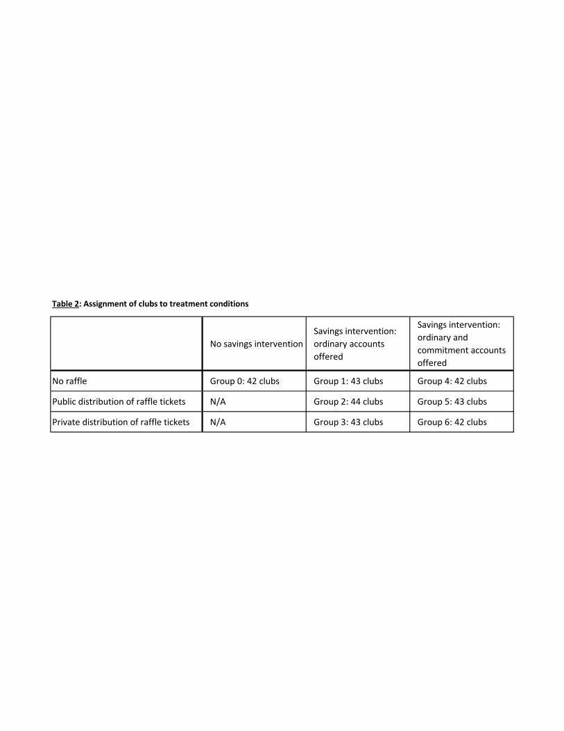
Table 2: Assignment of clubs to treatment conditions

No savings interventionSavings intervention: ordinary accounts offered

Savings intervention: ordinary and commitment accounts offered

No raffle Group 0: 42 clubs Group 1: 43 clubs Group 4: 42 clubs

Public distribution of raffle tickets N/A Group 2: 44 clubs Group 5: 43 clubs

Private distribution of raffle tickets N/A Group 3: 43 clubs Group 6: 42 clubs

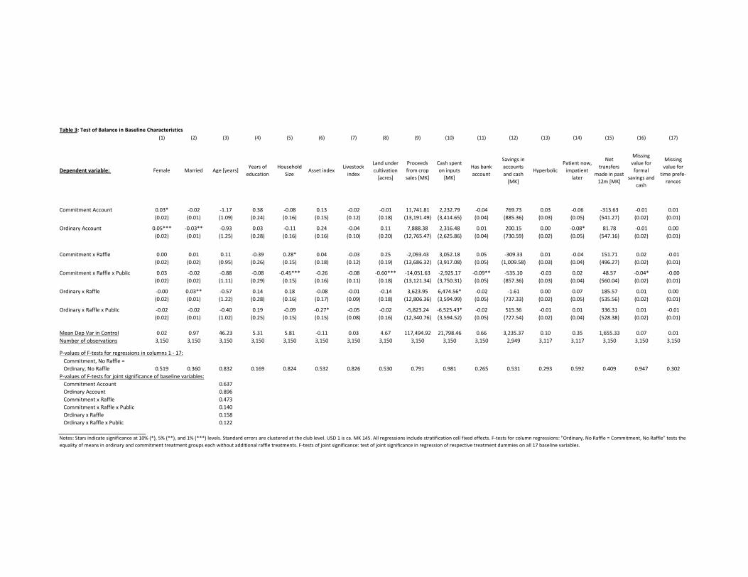
Table 3: Test of Balance in Baseline Characteristics(1) (2) (3) (4) (5) (6) (7) (8) (9) (10) (11) (12) (13) (14) (15) (16) (17)

Dependent variable:  Female Married Age [years]Years of education

Household Size

Asset indexLivestock index

Land under cultivation [acres]

Proceeds from crop sales [MK]

Cash spent on inputs [MK]

Has bank account

Savings in accounts and cash  [MK]

HyperbolicPatient now, impatient 

later

Net transfers 

made in past 12m [MK]

Missing value for formal 

savings and cash

Missing value for time prefe‐rences

Commitment Account 0.03* ‐0.02 ‐1.17 0.38 ‐0.08 0.13 ‐0.02 ‐0.01 11,741.81 2,232.79 ‐0.04 769.73 0.03 ‐0.06 ‐313.63 ‐0.01 0.01(0.02) (0.01) (1.09) (0.24) (0.16) (0.15) (0.12) (0.18) (13,191.49) (3,414.65) (0.04) (885.36) (0.03) (0.05) (541.27) (0.02) (0.01)

Ordinary Account 0.05*** ‐0.03** ‐0.93 0.03 ‐0.11 0.24 ‐0.04 0.11 7,888.38 2,316.48 0.01 200.15 0.00 ‐0.08* 81.78 ‐0.01 0.00(0.02) (0.01) (1.25) (0.28) (0.16) (0.16) (0.10) (0.20) (12,765.47) (2,625.86) (0.04) (730.59) (0.02) (0.05) (547.16) (0.02) (0.01)

Commitment x Raffle 0.00 0.01 0.11 ‐0.39 0.28* 0.04 ‐0.03 0.25 ‐2,093.43 3,052.18 0.05 ‐309.33 0.01 ‐0.04 151.71 0.02 ‐0.01(0.02) (0.02) (0.95) (0.26) (0.15) (0.18) (0.12) (0.19) (13,686.32) (3,917.08) (0.05) (1,009.58) (0.03) (0.04) (496.27) (0.02) (0.01)

Commitment x Raffle x Public 0.03 ‐0.02 ‐0.88 ‐0.08 ‐0.45*** ‐0.26 ‐0.08 ‐0.60*** ‐14,051.63 ‐2,925.17 ‐0.09** ‐535.10 ‐0.03 0.02 48.57 ‐0.04* ‐0.00(0.02) (0.02) (1.11) (0.29) (0.15) (0.16) (0.11) (0.18) (13,121.34) (3,750.31) (0.05) (857.36) (0.03) (0.04) (560.04) (0.02) (0.01)

Ordinary x Raffle ‐0.00 0.03** ‐0.57 0.14 0.18 ‐0.08 ‐0.01 ‐0.14 3,623.95 6,474.56* ‐0.02 ‐1.61 0.00 0.07 185.57 0.01 0.00(0.02) (0.01) (1.22) (0.28) (0.16) (0.17) (0.09) (0.18) (12,806.36) (3,594.99) (0.05) (737.33) (0.02) (0.05) (535.56) (0.02) (0.01)

Ordinary x Raffle x Public ‐0.02 ‐0.02 ‐0.40 0.19 ‐0.09 ‐0.27* ‐0.05 ‐0.02 ‐5,823.24 ‐6,525.43* ‐0.02 515.36 ‐0.01 0.01 336.31 0.01 ‐0.01(0.02) (0.01) (1.02) (0.25) (0.15) (0.15) (0.08) (0.16) (12,340.76) (3,594.52) (0.05) (727.54) (0.02) (0.04) (528.38) (0.02) (0.01)

Mean Dep Var in Control 0.02 0.97 46.23 5.31 5.81 ‐0.11 0.03 4.67 117,494.92 21,798.46 0.66 3,235.37 0.10 0.35 1,655.33 0.07 0.01Number of observations 3,150 3,150 3,150 3,150 3,150 3,150 3,150 3,150 3,150 3,150 3,150 2,949 3,117 3,117 3,150 3,150 3,150

P‐values of F‐tests for regressions in columns 1 ‐ 17:Commitment, No Raffle = Ordinary, No Raffle 0.519 0.360 0.832 0.169 0.824 0.532 0.826 0.530 0.791 0.981 0.265 0.531 0.293 0.592 0.409 0.947 0.302

P‐values of F‐tests for joint significance of baseline variables:Commitment Account 0.637Ordinary Account 0.896Commitment x Raffle 0.473Commitment x Raffle x Public 0.140Ordinary x Raffle 0.158Ordinary x Raffle x Public 0.122

Notes: Stars indicate significance at 10% (*), 5% (**), and 1% (***) levels. Standard errors are clustered at the club level. USD 1 is ca. MK 145. All regressions include stratification cell fixed effects. F‐tests for column regressions: "Ordinary, No Raffle = Commitment, No Raffle" tests the equality of means in ordinary and commitment treatment groups each without additional raffle treatments. F‐tests of joint significance: test of joint significance in regression of respective treatment dummies on all 17 baseline variables.

Table 4: Impact of Treatments on Deposits and Withdrawals

(1) (2) (3) (4) (5) (6) (7) (8) (9)

Dependent variable: 

Any Transfer via Direct Deposit 

(Take‐Up Indicator)

Total deposits into accounts [MK]

Total withdrawals from accounts 

[MK]

Deposits into ordinary accounts 

[MK]

Deposits into commitment accounts [MK]

Deposits into other accounts 

[MK]Net deposits [MK] Net deposits [MK] Net deposits [MK]

Time period:Mar 2009 ‐ Apr 

2010Mar‐Oct 2009 Mar‐Oct 2009 Mar‐Oct 2009 Mar‐Oct 2009 Mar‐Oct 2009 Mar‐Oct 2009 Nov‐Dec 2009 Jan‐Apr 2010

Commitment Account 0.21*** 21,861.22*** ‐20,740.45*** 19,464.30*** 1,993.55** 403.38 1,120.77* ‐1,065.54*** ‐255.61(0.05) (6,884.88) (6,829.20) (6,282.23) (788.59) (347.93) (669.29) (397.70) (351.51)

Ordinary Account 0.16*** 21,595.81*** ‐20,967.89*** 21,367.01*** ‐100.46 329.26 627.91 ‐941.67* 56.17(0.05) (7,073.18) (6,750.73) (6,962.06) (234.94) (278.44) (1,027.00) (481.11) (298.18)

Commitment x Raffle 0.03 ‐5,332.11 5,384.82 ‐4,453.27 ‐698.37 ‐180.46 52.71 ‐130.66 80.06(0.06) (7,847.77) (7,546.98) (7,192.16) (910.62) (366.93) (972.55) (655.39) (357.64)

Commitment x Raffle x Public ‐0.08 1,714.62 ‐1,315.18 1,781.13 ‐95.34 28.82 399.44 ‐254.58 39.32(0.06) (6,897.70) (6,509.39) (6,714.08) (548.96) (249.67) (928.21) (617.48) (201.25)

Ordinary x Raffle 0.01 ‐14,618.70** 14,965.51** ‐14,133.97* 1.19 ‐485.93* 346.81 434.73 ‐352.23(0 05) (7 365 53) (7 032 60) (7 274 39) (253 17) (271 10) (1 114 36) (544 91) (327 45)(0.05) (7,365.53) (7,032.60) (7,274.39) (253.17) (271.10) (1,114.36) (544.91) (327.45)

Ordinary x Raffle x Public 0.04 13,920.65* ‐15,155.79* 13,914.46* 45.42 ‐39.22 ‐1,235.14 ‐110.77 361.32(0.06) (7,829.14) (7,891.30) (7,777.86) (219.45) (120.20) (1,173.40) (401.48) (224.86)

Mean Dep Var in Control 0.000 3281.132 ‐3256.440 3107.045 0.000 174.087 24.692 ‐9.835 ‐147.938Number of observations 3,150 3,150 3,150 3,150 3,150 3,150 3,150 3,150 3,150

P‐value of F‐test:Commitment, No Raffle = Ordinary, No Raffle 0.333 0.977 0.979 0.826 0.009 0.846 0.678 0.817 0.440

Notes: Stars indicate significance at 10% (*), 5% (**), and 1% (***) levels. Standard errors are clustered at the club level. USD 1 is ca. MK 145. All regressions include stratification cell fixed effects and the following baseline variables: Dummy for male respondent; dummy for married; age in years; years of completed education; number of household members; asset index; livestock index; land under cultivation; proceeds from tobacco and maize sales during the 2008 season; cash spent on inputs for the 2009 season; dummy for ownership of any formal bank account; amount of savings in bank or cash (with missing values replaced with zeros); dummy for hyperbolic (missing values replaced with zeros); dummy for "patient now, impatient later" (missing values replaced with zeros); net transfers made to social network over 12 months; dummy for missing value in savings amount; dummy for missing value in hyperbolic and "patient now, impatient later". For complete variable definitions, see Appendix B. F‐tests: "Commitment, No Raffle = Ordinary, No Raffle" tests the equality of means in commitment and ordinary treatment groups each without additional raffle treatments. Planting season is Nov‐Apr. Fertilizer application occurs in Nov‐Dec. Fertilizer purchases occur in both pre‐planting period (Oct and before) and start of planting season (Nov‐Dec). Net deposits are deposits minus withdrawals.

Table 5: Impact of Treatments on Agricultural Outcomes in 2009‐2010 Season and Household Expenditure after 2010 Harvest

(1) (2) (3) (4) (5) (6)

Dependent variable: Land under cultivation 

[acres]Total value of inputs 

[MK]Proceeds from crop 

sales [MK]

Value of crop output (sold and not sold) 

[MK]

Farm profit (output‐input) [MK]

Total expenditure in 30 days prior to survey  [MK]

Commitment Account 0.42** 16,533.52** 22,962.78** 33,967.76** 19,205.08 1,859.77**(0.20) (6,394.38) (11,613.70) (15,115.21) (12,398.64) (856.78)

Ordinary Account 0.05 8,521.34 10,305.56 7,844.33 1,888.26 412.76(0.19) (6,272.71) (11,935.35) (14,805.72) (11,194.60) (876.40)

Commitment x Raffle ‐0.13 ‐8,507.97 11,704.31 ‐936.87 3,046.85 ‐532.12(0.19) (7,214.78) (13,774.27) (15,941.24) (13,481.03) (888.51)

Commitment x Raffle x Public ‐0.01 ‐1,381.03 ‐13,509.38 ‐6,340.87 184.16 ‐177.14(0.19) (6,224.95) (13,818.39) (15,460.54) (12,941.66) (968.76)

Ordinary x Raffle 0.25 ‐7,337.26 414.80 9,486.35 15,371.41 277.95(0.21) (6,571.42) (12,204.97) (15,159.76) (11,737.00) (979.02)

Ordinary x Raffle x Public 0.16 7,223.72 8,208.04 9,197.65 2,063.48 876.83(0.20) (5,865.43) (12,609.42) (15,750.11) (12,985.04) (873.19)

Mean Dep Var in Control 4.28 60371.80 91746.78 155684.93 95209.65 10678.42Number of observations 2,835 2,835 2,835 2,835 2,835 2,835

P‐value of F‐test:Commitment, No Raffle = Ordinary, No Raffle 0.057 0.276 0.297 0.081 0.142 0.141

0.0420.694

P‐value of F‐test of Ordinary=Commitment across regressions of columns 1,  2, 4 and 6: 0.254

Notes: Data come from the follow‐up survey conducted during July to September 2010. Stars indicate significance at 10% (*), 5% (**), and 1% (***) levels. Standard errors are clustered at the club level. USD 1 is ca. MK 145. All regressions include stratification cell fixed effects and the following baseline variables: Dummy for male respondent; dummy for married; age in years; years of completed education; number of household members; asset index; livestock index; land under cultivation; proceeds from tobacco and maize sales during the 2008 season; cash spent on inputs for the 2009 season; dummy for ownership of any formal bank account; amount of savings in bank or cash (with missing values replaced with zeros); dummy for hyperbolic (missing values replaced with zeros); dummy for "patient now, impatient later" (missing values replaced with zeros); net transfers made to social network over 12 months; dummy for missing value in savings amount; dummy for missing value in hyperbolic and "patient now, impatient later". For variable definitions, see Appendix B. F‐tests: "Commitment, No Raffle = Ordinary, No Raffle" tests the equality of means in commitment and ordinary treatment groups each without additional raffle treatments. F‐tests of "Ordinary=0" and "Ordinary=Commitment" are based on Seemingly Unrelated Regressions (SUR) estimation and test if the coefficient on Ordinary is jointly significantly different from zero and if the coefficient on Ordinary equals the coefficient on Commitment across regressions with independent variables from column 1, 2, 3 and 5.

P‐value of F‐test of Commitment= 0 across regressions of columns 1,  2, 4 and 6: P‐value of F‐test of Ordinary= 0 across regressions of columns 1,  2, 4 and 6:

Table 6: Impact of treatments on household size, transfers and fixed deposit demand

(1) (2) (3) (4) (5) (6)

Dependent variable:  Household sizeTotal transfers made [MK]

Total transfers received [MK]

Total net transfers made 

[MK]

Tobacco loan amount

Has fixed deposit account

Commitment Account 0.06 278.24 ‐490.38* 724.38* 3,686.22 0.06***(0.11) (330.70) (290.27) (405.43) (5,705.79) (0.02)

Ordinary Account 0.05 490.80 ‐205.87 641.82 4,508.14 0.03**(0.11) (352.28) (322.20) (436.42) (6,809.44) (0.02)

Commitment x Raffle 0.13 97.01 6.12 120.96 3,784.89 ‐0.02(0.12) (380.59) (251.87) (403.40) (6,552.34) (0.03)

Commitment x Raffle x Public ‐0.05 ‐118.62 512.32** ‐714.81* ‐8,524.39 0.01(0.12) (387.17) (257.67) (421.69) (6,613.50) (0.02)

Ordinary x Raffle 0.13 ‐556.49* ‐44.68 ‐445.54 ‐5,156.98 ‐0.03**(0.11) (333.87) (310.07) (442.23) (7,190.95) (0.02)

Ordinary x Raffle x Public 0.03 45.63 ‐156.28 148.57 5,578.51 0.02(0 11) (322 69) (293 52) (390 25) (6 728 23) (0 02)(0.11) (322.69) (293.52) (390.25) (6,728.23) (0.02)

Mean Dep Var in Control 5.72 2,871.70 2,492.13 417.89 40,147.26 0.04Number of observations 2,835 2,835 2,835 2,835 2,835 2,835

P‐value of F‐test:Commitment, No Raffle = Ordinary, No Raffle 0.952 0.553 0.299 0.846 0.903 0.250

Notes: Stars indicate significance at 10% (*), 5% (**), and 1% (***) levels. Standard errors are clustered at the club level. USD 1 is ca. MK 145. All regressions include stratification cell fixed effects and the following baseline variables: Dummy for male respondent; dummy for married; age in years; years of completed education; number of household members; asset index; livestock index; land under cultivation; proceeds from tobacco and maize sales during the 2008 season; cash spent on inputs for the 2009 season; dummy for ownership of any formal bank account; amount of savings in bank or cash (with missing values replaced with zeros); dummy for hyperbolic (missing values replaced with zeros); dummy for "patient now, impatient later" (missing values replaced with zeros); net transfers made to social network over 12 months; dummy for missing value in savings amount; dummy for missing value in hyperbolic and "patient now, impatient later". For  variable definitions, see Appendix B. F‐tests: "Commitment, No Raffle = Ordinary, No Raffle" tests the equality of means in commitment and ordinary treatment groups each without additional raffle treatments. 

Appendix Table 1: Attrition from Baseline to Endline Survey(A) (B)

Including Baseline Controls No Baseline controls

Dependent variable: Not interviewed during endline 

surveyNot interviewed during endline 

survey

Commitment Account 0.00 0.01

(0.02) (0.03)

Ordinary Account ‐0.00 0.00

(0.03) (0.03)

Commitment x Raffle ‐0.01 ‐0.02

(0.02) (0.02)

Commitment x Raffle x Public ‐0.00 0.01

(0.02) (0.02)

Ordinary x Raffle ‐0.03 ‐0.04

(0.02) (0.02)

Ordinary x Raffle x Public 0.05** 0.05**

(0.02) (0.02)

Mean Dep Var in Control 0.10 0.10

Number of observations 3,150 3,150

P‐value of F‐test:Commitment, No Raffle = Ordinary, No Raffle 0.802 0.790

Notes: Stars indicate significance at 10% (*), 5% (**), and 1% (***) levels. Standard errors are clustered at the club level. Regressions include stratification cell fixed effects. Column A includes the following baseline variables: Dummy for male respondent; dummy for married; age in years; years of completed education; number of household members; asset index; livestock index; land under cultivation; proceeds from tobacco and maize sales during the 2008 season; cash spent on inputs for the 2009 season; dummy for ownership of any formal bank account; amount of savings in bank or cash (with missing values replaced with zeros); dummy for hyperbolic (missing values replaced with zeros); dummy for "patient now, impatient later" (missing values replaced with zeros); net transfers made to social network over 12 months; dummy for missing value in savings amount; dummy for missing value in hyperbolic and "patient now, impatient later". For  variable definitions, see Appendix B. F‐tests: "Commitment, No Raffle = Ordinary, No Raffle" tests the equality of means in commitment and ordinary treatment groups each without additional raffle treatments. 

Appendix Table 2: Impact of Treatments on Deposits and WithdrawalsRegressions with stratification cell fixed effects but without additional baseline controls

(1) (2) (3) (4) (5) (6) (7) (8) (9)

Dependent variable: Any Transfer via 

Direct Deposit (Take‐Up Indicator)

Total deposits into accounts [MK]

Total withdrawals from accounts [MK]

Deposits into ordinary accounts 

[MK]

Deposits into commitment accounts [MK]

Deposits into other accounts [MK]

Net deposits [MK] Net deposits [MK] Net deposits [MK]

Time period: Mar 2009 ‐ Apr 2010 Mar‐Oct 2009 Mar‐Oct 2009 Mar‐Oct 2009 Mar‐Oct 2009 Mar‐Oct 2009 Mar‐Oct 2009 Nov‐Dec 2009 Jan‐Apr 2010

Commitment Account 0.22*** 23,454.54*** 22,350.21*** 21,061.32*** 1,981.98** 411.24 1,104.33 ‐1,090.51*** ‐276.00

(0.05) (7,191.44) (7,097.81) (6,544.53) (792.99) (351.68) (674.72) (411.08) (355.86)

Ordinary Account 0.17*** 23,180.20*** 22,507.50*** 22,927.66*** ‐77.07 329.61 672.70 ‐966.40* 50.70

(0.05) (7,845.12) (7,525.24) (7,744.01) (229.74) (263.08) (1,033.92) (491.51) (295.59)

Commitment x Raffle 0.03 ‐4,118.37 ‐4,295.93 ‐3,317.70 ‐660.97 ‐139.70 177.56 ‐201.21 48.24

(0.06) (7,950.51) (7,664.60) (7,265.29) (907.34) (384.74) (966.01) (644.27) (355.71)

Commitment x Raffle x Public ‐0.09 ‐2,516.49 ‐2,756.50 ‐2,264.35 ‐168.93 ‐83.21 240.01 ‐51.06 83.42

(0.06) (7,079.88) (6,699.59) (6,886.74) (558.89) (290.73) (944.96) (621.41) (201.39)

O di R ffl 0 00 13 795 20* 14 103 27* 13 265 82* 26 93 502 45** 308 07 377 09 426 26Ordinary x Raffle 0.00 ‐13,795.20* ‐14,103.27* ‐13,265.82* ‐26.93 ‐502.45** 308.07 377.09 ‐426.26

(0.05) (8,051.13) (7,732.94) (7,956.91) (248.51) (249.12) (1,099.16) (533.49) (320.09)

Ordinary x Raffle x Public 0.04 12,764.69 14,049.83* 12,712.39 78.64 ‐26.34 ‐1,285.14 ‐42.25 411.61*

(0.06) (8,291.97) (8,375.91) (8,230.31) (214.49) (117.53) (1,072.73) (397.27) (230.70)

Mean Dep Var in Control 0.00 3281.13 3256.44 3107.05 0.00 174.09 24.69 ‐9.84 ‐147.94

Number of observations 3,150 3,150 3,150 3,150 3,150 3,150 3,150 3,150 3,150

P‐value of F‐test:Commitment, No Raffle = Ordinary, No Raffle 0.361 0.978 0.987 0.844 0.010 0.829 0.721 0.824 0.430

Notes: Stars indicate significance at 10% (*), 5% (**), and 1% (***) levels. Standard errors are clustered at the club level. USD 1 is ca. MK 145. All regressions include stratification cell fixed effects. F‐tests: "Ordinary, No Raffle = Commitment, No Raffle" tests the equality of means in ordinary and commitment treatment groups without additional raffle treatments. Planting season is Nov‐Apr. Fertilizer application occurs in Nov‐Dec. Fertilizer purchases occur in both pre‐planting period (Oct and before) and start of planting season (Nov‐Dec). Net deposits are deposits minus withdrawals.

Apendix Table 3: Impact of Treatments on Agricultural Outcomes in 2009‐2010 Season and Household Expenditure after 2010 HarvestRegressions with stratification cell fixed effects but without additional baseline controls

(1) (2) (3) (4) (5) (6)

Dependent variable: Land under 

cultivation [acres]Total value of inputs 

[MK]Proceeds from crop 

sales [MK]

Value of crop output (sold and not sold) 

[MK]

Farm profit (output‐input) [MK]

Total expenditure in 30 days prior to survey  [MK]

Commitment Account 0.46** 18,560.76** 28,808.13** 41,143.38** 24,495.51* 2,260.29**

(0.23) (7,551.69) (13,661.24) (17,982.76) (13,772.67) (1,006.45)

Ordinary Account 0.11 10,922.89 15,407.48 15,223.08 7,219.16 831.83

(0.22) (7,049.34) (12,993.12) (15,827.62) (11,710.71) (955.61)

Commitment x Raffle ‐0.07 ‐7,451.19 11,076.62 ‐1,002.69 2,230.97 ‐378.69

(0.23) (8,679.48) (16,557.75) (19,841.45) (15,148.96) (1,038.19)

Commitment x Raffle x Public ‐0.29 ‐6,391.76 ‐22,797.51 ‐21,033.26 ‐9,902.10 ‐1,022.16

(0.22) (7,125.71) (16,227.86) (18,494.18) (14,733.64) (1,062.25)

Ordinary x Raffle 0.25 ‐5,402.06 2,431.04 11,251.43 15,159.52 398.97

(0.24) (7,647.77) (14,518.41) (17,862.93) (13,212.61) (1,042.70)

Ordinary x Raffle x Public 0.10 4,771.61 4,879.92 3,992.97 ‐857.43 524.17

(0.23) (6,659.53) (14,311.60) (17,745.21) (14,078.16) (883.06)

Mean Dep Var in Control 4.28 60371.80 91746.78 155684.93 95209.65 10678.42

Number of observations 2,835 2,835 2,835 2,835 2,835 2,835

P‐value of F‐test:Commitment, No Raffle = Ordinary, No Raffle 0.145 0.394 0.385 0.180 0.219 0.210

0.095

0.615

P‐value of F‐test of Ordinary=Commitment across regressions of columns 1,  2, 4 and 6: 0.563

Notes: Stars indicate significance at 10% (*), 5% (**), and 1% (***) levels. Standard errors are clustered at the club level. USD 1 is ca. MK 145. All regressions include stratification cell fixed effects. For complete variable definitions, see Appendix B. F‐tests: "Commitment, No Raffle = Ordinary, No Raffle" tests the equality of means in commitment and ordinary treatment groups each without additional raffle treatments. F‐tests of "Commitment=0", "Ordinary=0" and "Ordinary=Commitment" are based on Seemingly Unrelated Regressions (SUR) estimation and test if the coefficient on Commitment (Ordinary) is jointly significantly different from zero and if the coefficient on Ordinary equals the coefficient on Commitment across regressions with independent variables from columns 1, 3, 5 and 7.

P‐value of F‐test of Commitment= 0 across regressions of columns 1,  2, 4 and 6: 

P‐value of F‐test of Ordinary= 0 across regressions of columns 1,  2, 4 and 6:

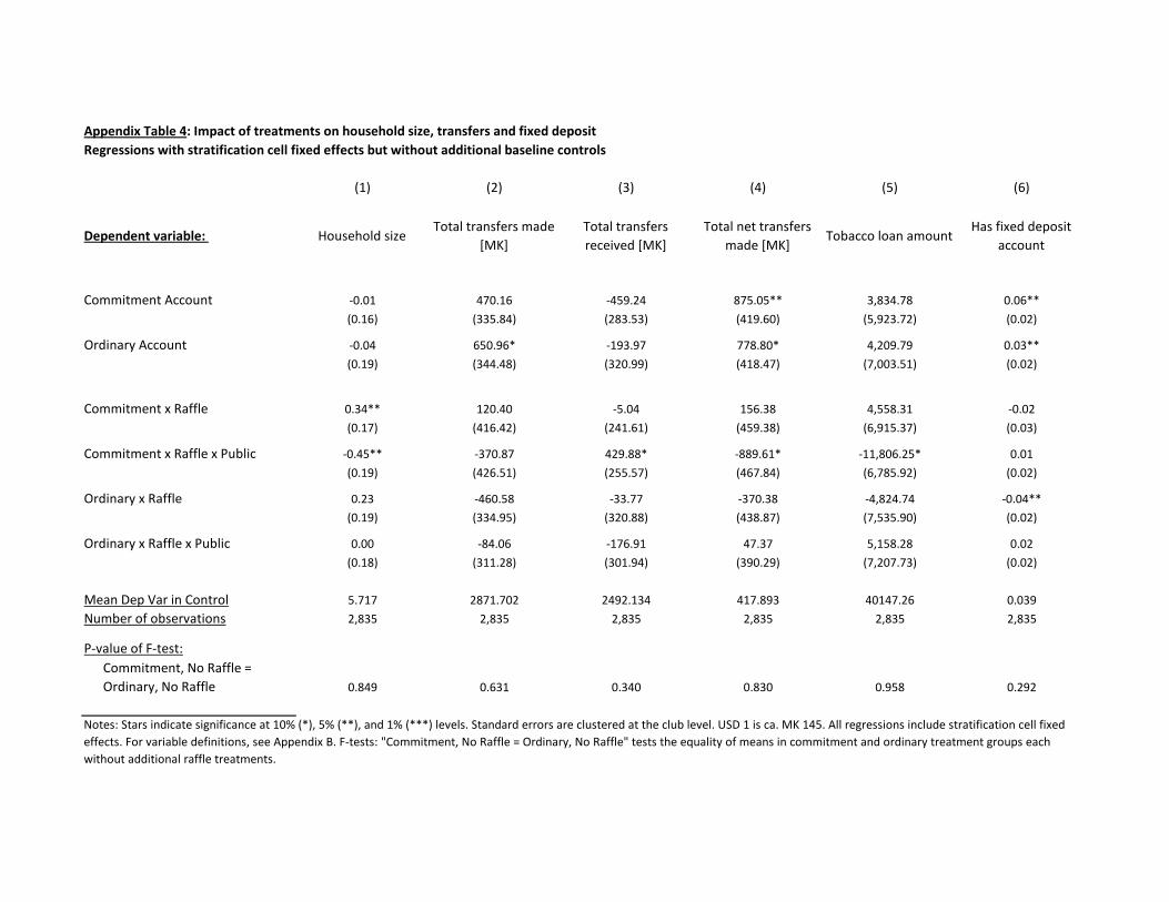
Appendix Table 4: Impact of treatments on household size, transfers and fixed depositRegressions with stratification cell fixed effects but without additional baseline controls

(1) (2) (3) (4) (5) (6)

Dependent variable:  Household sizeTotal transfers made 

[MK]Total transfers received [MK]

Total net transfers made [MK]

Tobacco loan amountHas fixed deposit 

account

Commitment Account ‐0.01 470.16 ‐459.24 875.05** 3,834.78 0.06**

(0.16) (335.84) (283.53) (419.60) (5,923.72) (0.02)

Ordinary Account ‐0.04 650.96* ‐193.97 778.80* 4,209.79 0.03**

(0.19) (344.48) (320.99) (418.47) (7,003.51) (0.02)

Commitment x Raffle 0.34** 120.40 ‐5.04 156.38 4,558.31 ‐0.02

(0.17) (416.42) (241.61) (459.38) (6,915.37) (0.03)

Commitment x Raffle x Public ‐0.45** ‐370.87 429.88* ‐889.61* ‐11,806.25* 0.01

(0.19) (426.51) (255.57) (467.84) (6,785.92) (0.02)

Ordinary x Raffle 0 23 ‐460 58 ‐33 77 ‐370 38 ‐4 824 74 ‐0 04**Ordinary x Raffle 0.23 460.58 33.77 370.38 4,824.74 0.04

(0.19) (334.95) (320.88) (438.87) (7,535.90) (0.02)

Ordinary x Raffle x Public 0.00 ‐84.06 ‐176.91 47.37 5,158.28 0.02

(0.18) (311.28) (301.94) (390.29) (7,207.73) (0.02)

Mean Dep Var in Control 5.717 2871.702 2492.134 417.893 40147.26 0.039

Number of observations 2,835 2,835 2,835 2,835 2,835 2,835

P‐value of F‐test:Commitment, No Raffle = Ordinary, No Raffle 0.849 0.631 0.340 0.830 0.958 0.292

Notes: Stars indicate significance at 10% (*), 5% (**), and 1% (***) levels. Standard errors are clustered at the club level. USD 1 is ca. MK 145. All regressions include stratification cell fixed effects. For variable definitions, see Appendix B. F‐tests: "Commitment, No Raffle = Ordinary, No Raffle" tests the equality of means in commitment and ordinary treatment groups each without additional raffle treatments.