combustione turbolenta ed emissioni - unina.itwpage.unina.it/anddanna/capri/capri...
TRANSCRIPT
Combustione turbolenta edemissioni
Alessio FrassoldatiDip. CMIC – Politecnico di Milano
Corso di Dottorato congiunto Polimi-Federico II Chimica e fluidodinamica della combustione
Anacapri: 5-9 Ottobre 2009

Combustione turbolenta ed emissioni 2
Outline
1. Introduction: interactions between turbulence and chemistry
2. Numerical modeling of nitrogen oxides formation in turbulent flames: Kinetic Post Processor
4. Numerical modeling of soot formation in turbulent non premixed flames
5. Conclusions
3. Application examples

Combustione turbolenta ed emissioni 3
Emissions regulations
Increasingly stringent regulations for Pollutant emissions
in furnaces, power plants, gas turbines, burners etc.
Global NOx levels - SCIAMACHY satellite in 2004.

Combustione turbolenta ed emissioni 4
NOx regulations and targets for 2020

Combustione turbolenta ed emissioni 5
C 2H6
C 2H5
C 2H4
C 2H3
C 2H2
Aromatics
Soot
Pyrolysis
O2
CH i
O2
OH
Oxidation
CH 3OOH
CH 3OH
CH 2OH
CH 3OO
CH 3
CH 3O
CH 2O
HCO
CO
CO 2
CH 4
CH4 + 2O2 →→→→ CO2 + 2 H2O
NOx
O2 + N2
Combustion: a complex chemical process
Huge number of reactions and different timescales
time [s]
norm
aliz
ed m
ass
fra
ctio
n

Combustione turbolenta ed emissioni 6
SOxSOx
......
nC7-iC8nC7-iC8
C6C6
C3C3
C2C2
CH4CH4
COCO
H2-O2H2-O2
NOxNOx
SootSoot
PAHPAH
Chlorinatedspecies
Chlorinatedspecies
Kinetic mechanism includes hydrocarbons up to Diesel
and jet fuels as well as several pollutants
- Hierachy
- Modularity
- Generality
Detailed kinetic mechanism of combustion
~ 400 species
~ 12000 reactions
http://www.chem.polimi.it/CRECKModeling/

Combustione turbolenta ed emissioni 7
NOx formation chemically controlled
NOx in a laminar premixed flame H2
(Warnatz, 1981)
10
100
1000
0.25 0.35xH2
pp
m N
Ox
Equilibrium
Combustione turbolenta ed emissioni 8
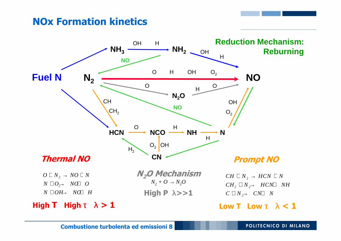
NON2H OH O2O
O N NO N
N O NO O
N OH NO H
+ → ++ → ++ → +
2
2
Thermal NO
High T High ττττ λλλλ > 1
HCN NCO NH N
CH
CH2
O H
H
OH
O2
CH N HCN N
CH N HCN NH
C N CN N
+ → ++ → +
+ → +
2
2 2
2
Prompt NO
Low T Low ττττ λλλλ < 1
NH2 OHH
OH HNH3
Fuel N
OHO2
CNH2
NO
NO
Reduction Mechanism:Reburning
N2O
O OH
N2O MechanismN2 + O → N2O
High P λλλλ>>1
NOx Formation kinetics
Combustione turbolenta ed emissioni 9
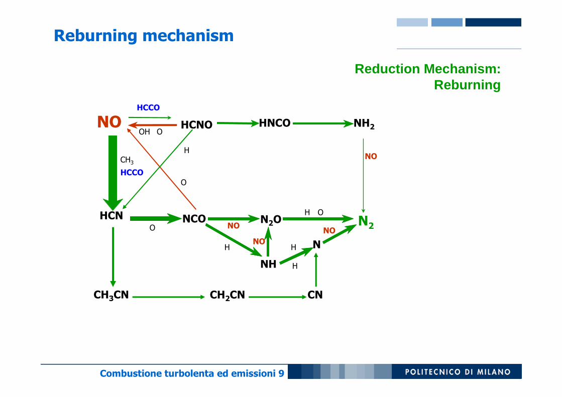
Reduction Mechanism:Reburning
Reburning mechanism
HCN
NO
O NO
NO
NO
H
H O
H
O
H
HCCO
HCCO
NO
N2
HCNO HNCO
NCO N2O
NH
N
NH2
CH3
OOH
H
CH3CN CH2CN CN
Combustione turbolenta ed emissioni 10
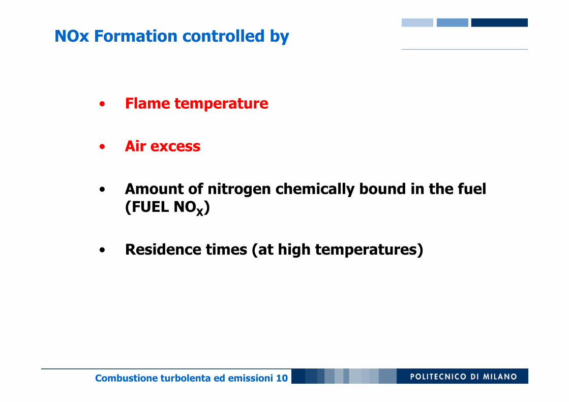
• Flame temperature
• Air excess
• Amount of nitrogen chemically bound in the fuel (FUEL NOX)
• Residence times (at high temperatures)
NOx Formation controlled by

Combustione turbolenta ed emissioni 11
Air excess (1/Φ)
NO
x
T
1
Rich Conditions
Lean conditions
Lawconstraints
T and ΦΦΦΦ effect on NOx formation
Combustione turbolenta ed emissioni 12
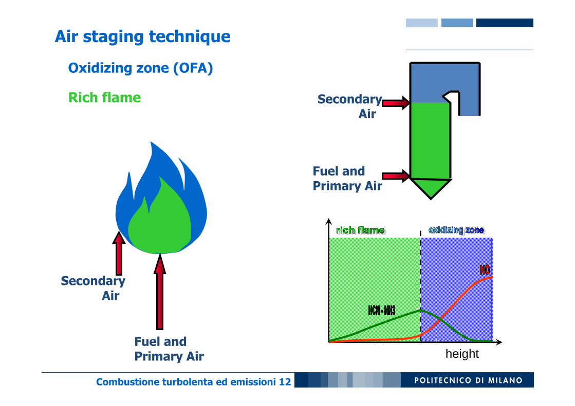
Fuel andPrimary Air
SecondaryAir
heightFuel andPrimary Air
SecondaryAir
Oxidizing zone (OFA)
Rich flame
Air staging technique
Combustione turbolenta ed emissioni 13
height
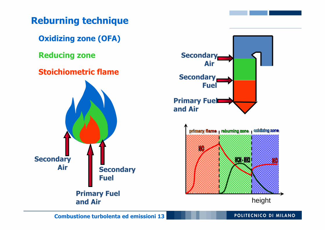
Primary Fueland Air
SecondaryAir
Secondary Fuel
Primary Fueland Air
SecondaryAir Secondary
Fuel
Oxidizing zone (OFA)
Reducing zone
Stoichiometric flame
Reburning technique

Combustione turbolenta ed emissioni 14
Pollutant formation in turbulent flames
Chemistry
Slow chemistry
Finite-ratechemistry
Fast chemistry
Fluid-dynamics
Kolmogorovlenght
Meanresidence time
ττττ (s)
103
100
102
101
10-1
10-4
10-2
10-3
10-5
10-8
10-6
10-7
10-9
NOx
SootPAH
CO
Mixed -Burned
Perfectmixing
Adapted from: R. Fox , “Computational models for turbulent reacting flows”, Cambridge University Press
(2002)
For PAH and soot the decoupling between chemistry and fluid
dynamics is not possible
time [s]
norm
aliz
ed m
ass
frac
tion
Turbulence-kinetics interactions
Combustione turbolenta ed emissioni 15
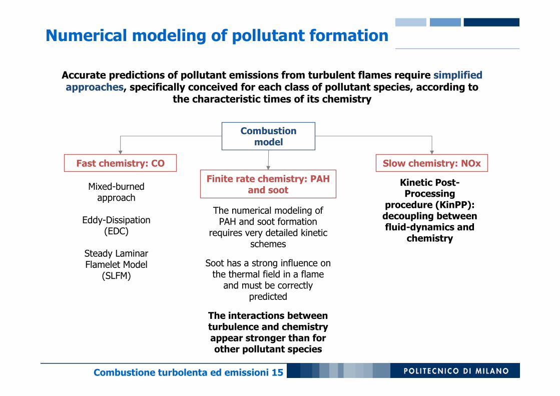
Accurate predictions of pollutant emissions from turbulent flames require simplified approaches, specifically conceived for each class of pollutant species, according to
the characteristic times of its chemistry
Combustion model
Finite rate chemistry: PAH and soot
Fast chemistry: CO Slow chemistry: NOx
Mixed-burned approach
Eddy-Dissipation (EDC)
Steady Laminar Flamelet Model
(SLFM)
The numerical modeling of PAH and soot formation
requires very detailed kinetic schemes
Soot has a strong influence on the thermal field in a flame
and must be correctly predicted
The interactions between turbulence and chemistry appear stronger than for other pollutant species
Kinetic Post-Processing
procedure (KinPP): decoupling between fluid-dynamics and
chemistry
Numerical modeling of pollutant formation
Combustione turbolenta ed emissioni 16
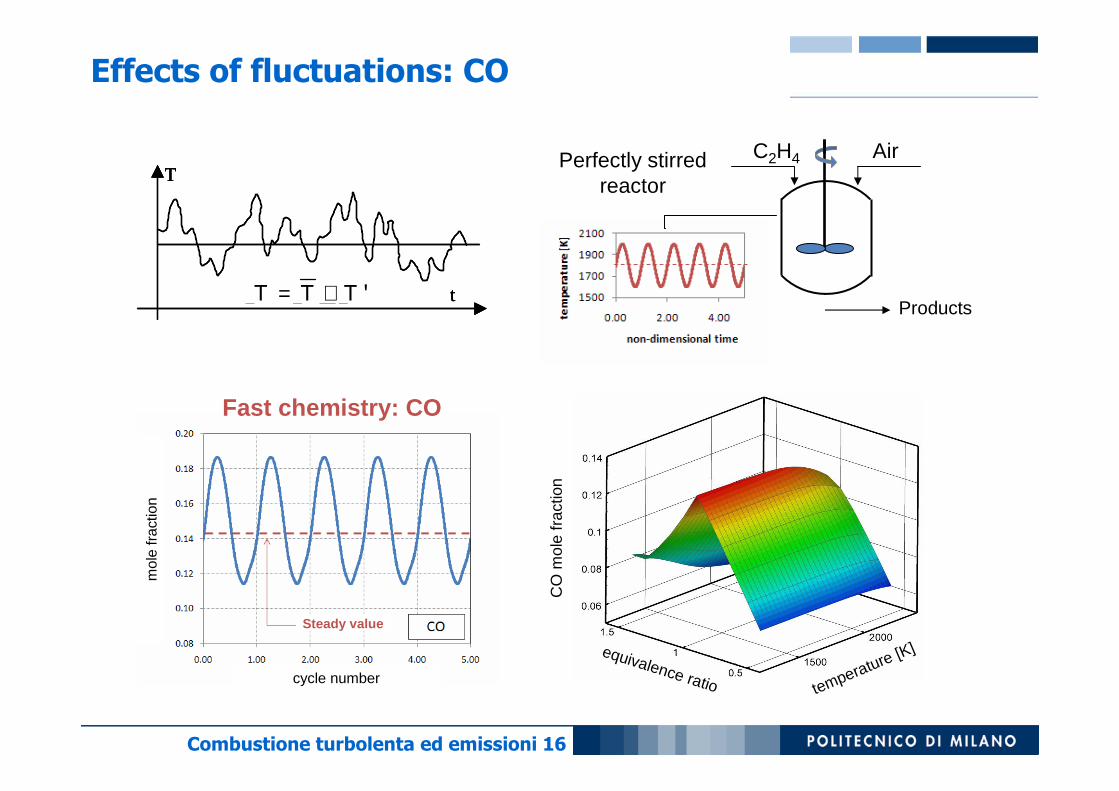
C2H4 Air
Products
Perfectly stirred reactor
Fast chemistry: CO
T
t
T
t'T T T= +
T
t
T
t'T T T= +T T T '= +
temperature [K]equivalence ratio
CO
mol
e fr
actio
n
cycle number
mol
e fr
actio
n
Steady value
Effects of fluctuations: CO

Combustione turbolenta ed emissioni 17
temperature [K]equivalence ratio
soot
vol
ume
frac
tion
[ppm
]
temperature [K]equivalence ratio
NO
mol
e fr
actio
n
Slow chemistry:NO
cycle number
mol
e fr
actio
n
Finite-rate chemistry: Soot
cycle number
volu
me
frac
tion
Steady value
Steady value
Effects of fluctuations: NO and Soot
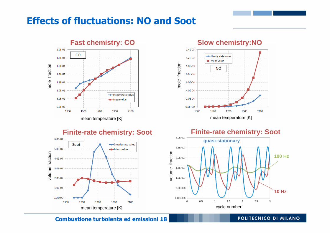
Combustione turbolenta ed emissioni 18
Finite-rate chemistry: Soot
mean temperature [K]
volu
me
frac
tion
Fast chemistry: CO
mean temperature [K]
mol
e fr
actio
nSlow chemistry:NO
mean temperature [K]
mol
e fr
actio
n
0 0.5 1 1.5 2 2.5 30.0E+000
5.0E-008
1.0E-007
1.5E-007
2.0E-007
2.5E-007
3.0E-007
cycle number
volu
me
frac
tion
quasi-stationary
100 Hz
10 Hz
cycle number
volu
me
frac
tion
Finite-rate chemistry: Soot
Effects of fluctuations: NO and Soot

Combustione turbolenta ed emissioni 19
Pollutants emissions (NOx): modeling review
Different levels of detail are possible:
There are currently several techniques used in practice to predict the emissions from real combustors.
They fall into three general categories:
• Empirical and semi-empirical models
• Simplified physics-based models
• Detailed models
Each method has strengths and weaknesses and will be briefly discussed

Combustione turbolenta ed emissioni 20
Empirical models are very simple and the least computationally intensive.
Require empirically determined constants and are useful for correlating known historical NOx emissions for a specific combustor.
1-Empirical models
Since empirical models are generated from fitting a certain number of constants using historical data, they cannot be expected to perform well when the combustor undergoes a design change.
[D.L. Allaire – Thesis, MIT, 2006]

Combustione turbolenta ed emissioni 21
2-Simplified Physics-based models
D.L. Allaire - MIT
Primary zone modeled using 16 parallel PSRs
PFR for other zones

Combustione turbolenta ed emissioni 22
2-Simplified Physics-based models
D.L. Allaire - MIT
Problem: it is necessary to define parameters: Primary zone Unmixedness, Temperature and dimensions of the PFRs
It represent the level of mixing between fuel and air in the primary zone
Sensitivity of the results to this parameter -> tuned using experimental data obtained in some operating conditions
Only CO and NO
Combustione turbolenta ed emissioni 23
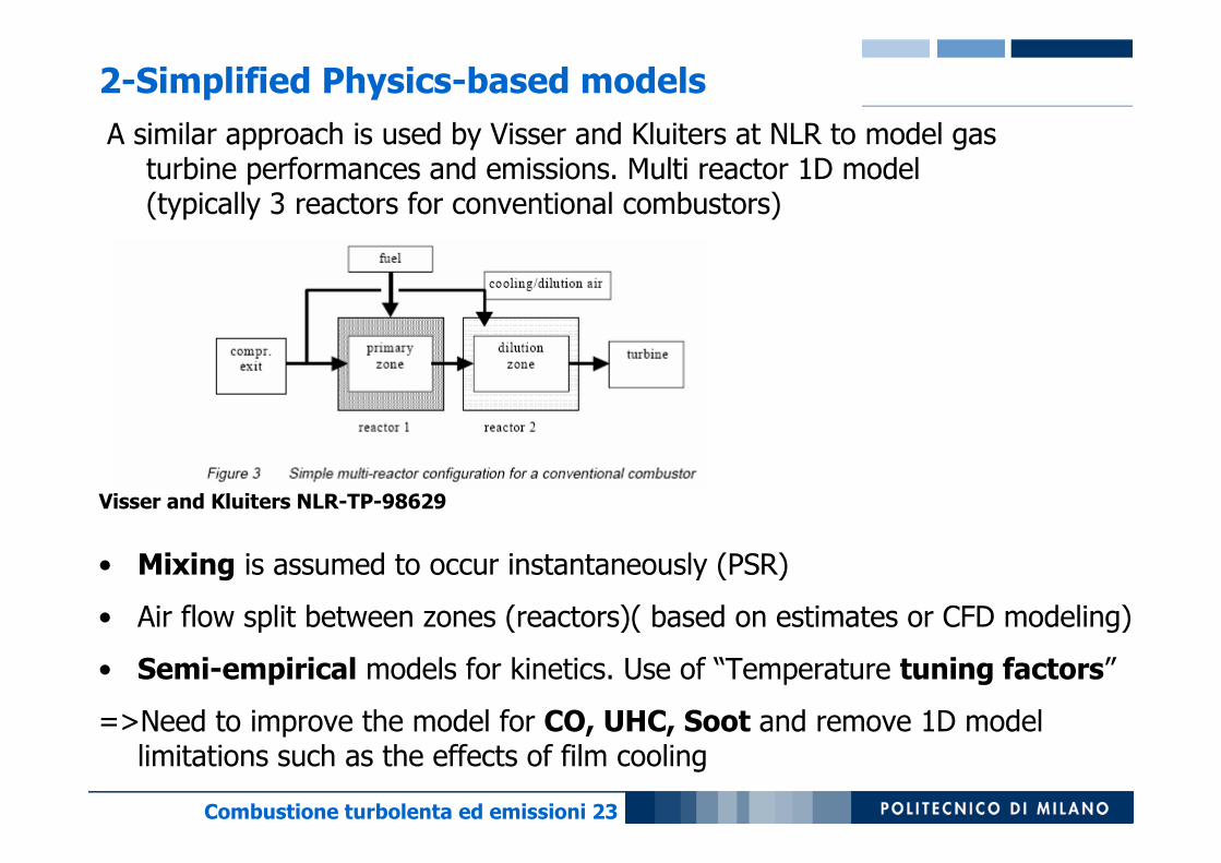
2-Simplified Physics-based models
A similar approach is used by Visser and Kluiters at NLR to model gas turbine performances and emissions. Multi reactor 1D model (typically 3 reactors for conventional combustors)
Visser and Kluiters NLR-TP-98629
• Mixing is assumed to occur instantaneously (PSR)
• Air flow split between zones (reactors)( based on estimates or CFD modeling)
• Semi-empirical models for kinetics. Use of “Temperature tuning factors”
=>Need to improve the model for CO, UHC, Soot and remove 1D model limitations such as the effects of film cooling
Combustione turbolenta ed emissioni 24
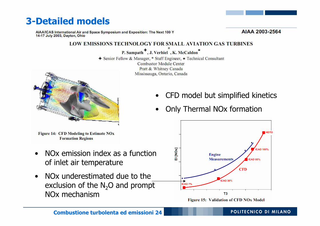
3-Detailed models
• CFD model but simplified kinetics
• Only Thermal NOx formation
• NOx emission index as a function of inlet air temperature
• NOx underestimated due to the exclusion of the N2O and prompt NOx mechanism

Combustione turbolenta ed emissioni 25
Chemistry
Slow chemistry
Finite-ratechemistry
Fast chemistry
Fluid-dynamics
Kolmogorovscale
Meanresidence
time
ττττ(s)
103
100
102
101
10-1
10-4
10-2
10-3
10-5
10-8
10-6
10-7
10-9
NOx
Soot
CO
Mixed - Burned
Perfect mixing
It is still unfeasible to directly couple fluid dynamics and detailed kinetic
Pollutant species (such as NOx) affect only marginally
the main combustion process and consequently do not influence the overall temperature and flow field
The prediction of pollutant species (NOx) can be decoupled from the
CFD simulation
Kinetic Post Processor (KinPP)
NOx => Kinetic Post Processor

Combustione turbolenta ed emissioni 26
The problem:CPU time in CFD ∝ N 2Species or N 3Species
Memory used in CFD ∝ N Species
⇒ Kinetic mechanisms adopted in CFD simulations of industrial interest (3D) refer to a few chemical species
But:Chemical kinetics is absolutely necessary to predict pollutant formation (ppm or ppb)
⇒ Detailed mechanisms have to be adopted
Good news: Pollutants are present in traces and (generally) do not influence the velocity and temperature fields
⇒ Emission predictions (NOx) can be de-coupled from CFD computation
⇒ Kinetic Post Processor (KPP)
Faravelli, T., Frassoldati, A., Ranzi, E., Comb Flame, 135:97 (2003)
3-Detailed models: KPP

Combustione turbolenta ed emissioni 27
Kinetic Post Processor: advantages
The Kinetic Post-processor:�assumes the temperature and flow fields as predicted by the CFD.
�solves mass balances in the cells with detailed chemistry at fixed temperature. Each cell is a PSR reactor.
Advantages over direct coupling of CFD and Detailed Kinetics
� possibility to group several cells. Clustering equivalent cells reduces the dimensions of the problem.
� fix the temperature inside the cells. This reduces the high non linearity of the system, mainly related to the reaction rates and to the coupling between mass and energy balances.

Combustione turbolenta ed emissioni 28
µ= − ⋅ ∇ωr
ti i
t
JSc
Diffusion flux due to concentration gradientsand velocity fluctuations of the turbulent flow
ConvectionChemicalreactionsDiffusion
Turbulentdiffusion
ConvectiveTransport
1 1
0ω ω ν= =
⋅ − ⋅ + + ⋅ ⋅ + = ∑ ∑*,
Ns Nrin outi i i n n i ij j i
n j
W W J S V M r S
Mass balance for a single reactor
Non linear system of equations
Number of equations: Nspecies x Nreactors
1 4
22 13λ λ
νεγ γ = ⋅ =
/
* .V Vk
The effective volume V* available for chemical reactions is evaluated according
to the EDC model
Reactor network
EvaporationDevolatilization
Combustione turbolenta ed emissioni 29
T
t
T
t'T T T= +
T
t
T
t'T T T= +T T T '= +
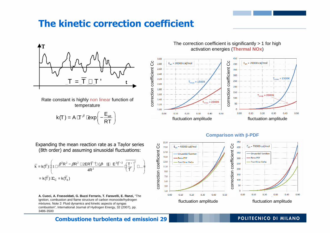
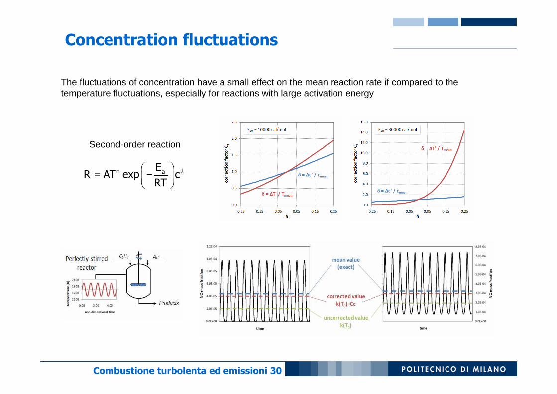
Expanding the mean reaction rate as a Taylor series(8th order) and assuming sinusoidal fluctuations:
The correction coefficient is significantly > 1 for high activation energies (Thermal NOx )
22 2 2 1 2 2
2
2 11
4
( ) '( ) ...
= ( ) ( )C k
R R ERT E T Tk k T
TR
k T C k T
β β β− − − + ⋅ − + = ⋅ + ⋅ + =
⋅ =
Rate constant is highly non linear function oftemperature
( ) exp attEk T A T
RTβ = ⋅ ⋅ −
The kinetic correction coefficient
fluctuation amplitude
corr
ectio
n co
effic
ient
Cc
corr
ectio
n co
effic
ient
Cc
fluctuation amplitude
fluctuation amplitude
corr
ectio
n co
effic
ient
Cc
fluctuation amplitude
corr
ectio
n co
effic
ient
Cc
Comparison with β-PDF
A. Cuoci, A. Frassoldati, G. Buzzi Ferraris, T. Fara velli, E. Ranzi, “The ignition, combustion and flame structure of carbon monoxide/hydrogen mixtures. Note 2: Fluid dynamics and kinetic aspects of syngascombustion”, International Journal of Hydrogen Energy, 32 (2007), pp. 3486-3500
Combustione turbolenta ed emissioni 30
The fluctuations of concentration have a small effect on the mean reaction rate if compared to the temperature fluctuations, especially for reactions with large activation energy
= −
n 2aER AT exp c
RT
Second-order reaction
Concentration fluctuations
Combustione turbolenta ed emissioni 31
The numerical problem
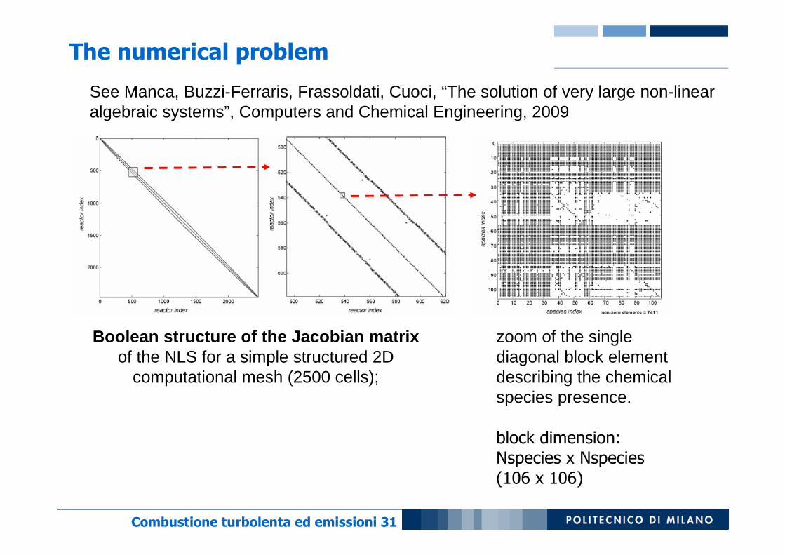
See Manca, Buzzi-Ferraris, Frassoldati, Cuoci, “The solution of very large non-linearalgebraic systems”, Computers and Chemical Engineering, 2009
Boolean structure of the Jacobian matrixof the NLS for a simple structured 2D
computational mesh (2500 cells);
zoom of the single diagonal block element describing the chemical species presence.
block dimension:Nspecies x Nspecies(106 x 106)

Combustione turbolenta ed emissioni 32
CFD Results ⇒ First guess solution
Newton’s method
OK
YesNo
Time integration (ODE)
Low residuals in all equationsYes
No
Global Newton’s method
OK
Yes NoTime integration (ODE)
Solution Low pollutant concentrations (ppm)Need of very low residuals (Newton’s method)
KPP: numerical solution of a large NLS
Local solution in each “reactor”
Global solution for all “reactors”

Combustione turbolenta ed emissioni 33
Convergence of the numerical method
Convergence behavior during the iterative solution and effect of the global Newton’s method.

Combustione turbolenta ed emissioni 34
CO / H2 / N2 Jet Flames 1
Unconfined turbulent jet flame in low-velocity coflow
Fuel composition:
40% CO, 30% H2, 30% N2
Fuel inlet velocity: ~ 45-76 m/s
Air Fuel
Computational domain
Non uniform, structured mesh
About 42000 cells (320x130)
High resolution in the region close to the inlets
Com
bust
ion
cham
ber
CFD Simulation details
CFD Code FLUENT 6.3.2
Space 2D Axial-Symmetric
Time Steady
Turbulence modeling Standard κ-ε turbulence model
Wall treatment Standard wall functions
Radiation Discrete Ordinate Model
Solver Segregated implicit solver
Spatial resolution Second-Order Upwind scheme
Pressure Interpolation PRESTO!
Combustion model
Eddy Dissipation (ED)
Steady Laminar Flamelets (SLF)
Eddy Dissipation Concept (EDC)
1 Barlow, R.S., et al., Sandia/ETH-Zurich CO/H2/N2 Flame Data - Release 1.1.
www.ca.sandia.gov/TNF, Sandia National Laboratories, 2002
Experimental flames

Combustione turbolenta ed emissioni 35
The best agreement with experimental measurements is obtained for the EDC model
CFD simulations: comparison with exp data (Sandia Syngas jet flame)
temperature CO2 mass fraction
SLFM
EDEDC
SLFM
EDEDC
temperatureaxial velocityturbulent kinetic energy
Temperature[K]
axial coordinate [mm]
tem
pera
ture
[K]
radial coordinate [mm]
turb
ulen
t kin
etic
ene
rgy
[m2/
s]
radial coordinate [mm]
velo
city
[m/s
]
axial coordinate [mm]
tem
pera
ture
[K]
axial coordinate [mm]
mas
s fr
actio
n

Combustione turbolenta ed emissioni 36
KPP: NOx predictions
NO mass fraction Axial profiles
axial coordinate [mm]
NO
mas
s fr
actio
n
axial coordinate [mm]
NO
mas
s fr
actio
nradial coordinate [mm]
NO
mas
s fr
actio
n
radial coordinate [mm]N
O m
ass
frac
tion
Radial profiles
Barlow, R.S., et al. , Sandia/ETH-Zurich CO/H2/N2
Flame Data - Release 1.1. www.ca.sandia.gov/TNF, Sandia National Laboratories, 2002

Combustione turbolenta ed emissioni 37
NOx scatter plots
NO mass fraction
OH mass fraction
the effect is less relevant than for NO as a consequence of the lower apparent activation energy of OH radicals formation process
the predicted NO profile obtained when suppressing the effect of temperature fluctuations lies at the lower boundary of the scatter plot, especially close to the fuel inlet
mixture fraction
NO
mas
s fr
actio
n
mixture fraction
NO
mas
s fr
actio
n
mixture fraction
OH
mas
s fr
actio
n
mixture fraction
OH
mas
s fr
actio
n

Combustione turbolenta ed emissioni 38
Parente et al., European Combustion Meeting 2009 14-17 April 2009 - Vienna, Austria
rad
ian
t tu
be
flam
e tu
be
fuel inlet
air inlet
window
FA [s] T [K] |V| [m/s]
20 30 40 50 60 70 8020
30
40
50
60
70
80
NO [ppm] - Exp.
NO
[ppm
] - N
um.
CFD simulation
(FLUENT 6.3.26)
Case 2.
Mesh 9500 cells
NOx prediction (KPP)
Application example: FLOX® Burner

Combustione turbolenta ed emissioni 39
Numerical efficiency
Different techniques are used to reduce the CPU time
1) Fluid Age : The idea is to take into account the relevant physical phenomena, i.e. solving the individual reactors according to their f luid age (FA).The age on an element of fluid is the time elapsed since it entered the computational domain. This has an impact on the iterative solution which is accelerated because of the higher convergence speed. FA can be easily calculated by CFD codes and describes how the fluid flows inside the domain.
2) Analytical Jacobian Matrix : the numerical solution of large NLS involves computing Jacobian matrices several times, making the computation of derivatives a central and time-consuming partof the solution process. =>the derivatives of kinetic rate equations are evaluated analytically rather than numerically. The MATLAB differentiation toolbox was used to calculate the analytical derivatives , which are then directly included and compiled in the C++ routines of the KPP code . This calculation is needed only one time for each mechanism and takes less than 1 h on a PC.
3) Parallel computing : work in progress….
Speed ×××× 8
Speed ×××× 1.3
Combustione turbolenta ed emissioni 40
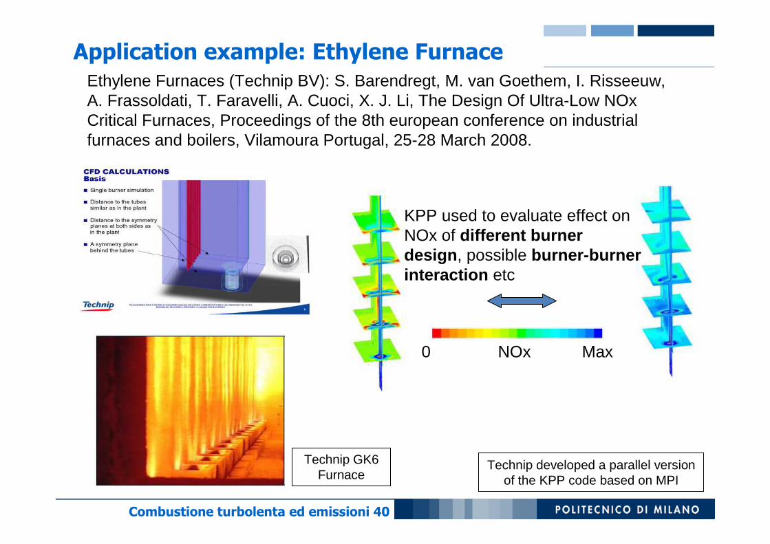
Ethylene Furnaces (Technip BV): S. Barendregt, M. van Goethem, I. Risseeuw, A. Frassoldati, T. Faravelli, A. Cuoci, X. J. Li, The Design Of Ultra-Low NOxCritical Furnaces, Proceedings of the 8th european conference on industrial furnaces and boilers, Vilamoura Portugal, 25-28 March 2008.
Technip developed a parallel versionof the KPP code based on MPI
KPP used to evaluate effect on NOx of different burnerdesign , possible burner-burnerinteraction etc
Application example: Ethylene Furnace
NOx0 Max
Technip GK6 Furnace

Combustione turbolenta ed emissioni 41
Temperature [800÷2500 K]
NO2 [0÷160 ppm]NO [0÷2300 ppm]
[min ÷ max]
Main(LPP)
Pilot
Temperature [800÷2500 K]
NO2 [0÷160 ppm]NO [0÷2300 ppm]
[min ÷ max][min ÷ max]
Main(LPP)
Pilot
experimental analysis:
CLEAN and NEWAC combustors studied at Karlsruhe University, ONERA
modeling activity
CFD CodeAVIO BODY 3D
Kinetic Post Processor
Application example: Gas Turbines
Gas Turbine for Aero-engines (Frassoldati, Cuoci, F aravelli, Ranzi, Colantuoni, Di Martino, Cinque, Comb Sci Tech,181:483, 2009)
Combustione turbolenta ed emissioni 42
CLEAN combustor
Pilot Run Stage Burning Full Running
Main Stage (LPP)
Pilot
ICAO 7% ICAO 30% ICAO 85-100%
Outerliner
Innerliner
Dilutionholes
Pilot Run Stage Burning Full Running
Main Stage (LPP)
Pilot
ICAO 7% ICAO 30% ICAO 85-100%
Pilot Run Stage Burning Full Running
Main Stage (LPP)
Pilot
ICAO 7% ICAO 30% ICAO 85-100%
Outerliner
Innerliner
Dilutionholes
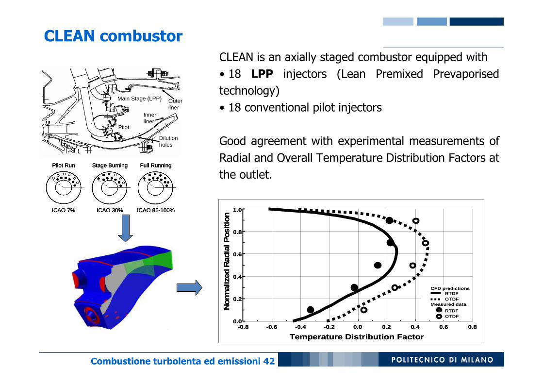
CLEAN is an axially staged combustor equipped with
• 18 LPP injectors (Lean Premixed Prevaporised
technology)
• 18 conventional pilot injectors
Good agreement with experimental measurements of
Radial and Overall Temperature Distribution Factors at
the outlet.
0.0
0.2
0.4
0.6
0.8
1.0
-0.8 -0.6 -0.4 -0.2 0.0 0.2 0.4 0.6 0.8
Temperature Distribution Factor
Nor
mal
ized
Rad
ialP
ositi
on
CFD predictions
Measured data
RTDFOTDF
RTDFOTDF
0.0
0.2
0.4
0.6
0.8
1.0
-0.8 -0.6 -0.4 -0.2 0.0 0.2 0.4 0.6 0.8
Temperature Distribution Factor
Nor
mal
ized
Rad
ialP
ositi
on
CFD predictions
Measured data
RTDFOTDF
RTDFOTDF

Combustione turbolenta ed emissioni 43
CLEAN combustor: KPP simulation
[min ÷ max]
Temperature [800÷2500 K]
NO2 [0÷160 ppm]NO [0÷2300 ppm]
Main(LPP)
Pilot
Formation of NO2 in the low temperature region (film cooling)
Different amounts of NOx formed in the conventional (pilot) and LPP injectors
0
100
200
300
400
500
600
0 20 40 60 80 100 120 140 160 180 200 220 240Angular position [deg]
NO
x E
mis
sion
s [p
pm]
NO
NO2Possible NO→NO2conversion in the probe

Combustione turbolenta ed emissioni 44
NEWAC combustor
Fuel
(Pilot line)
Fuel
(Main line)
Studied the performance of the PERM injection system in a simple tubular combustor
(Partial Evaporation & Rapid Mixing). Exp Data from UNI Karlsrhue
15%Pilot Fuel/Total Fuel
18÷32Air/Fuel Ratio (AFR)
506÷522Combustor Inlet Temperature [K]
8Combustor Inlet Pressure [bar]
Operating Conditions
(Frassoldati, Cuoci, Faravelli, Ranzi, Colantuoni, Di Martino, Cinque, Kern, Marinov, Zarzalis, Medite rranean Combustion Symposium 2009)

Combustione turbolenta ed emissioni 45
NEWAC combustor: effect of pressure
Good agreement with measured emissions: higher pressure and air preheat significantly increases emissions (∼2 orders of magnitude)
P = 8 Bar, Tair inlet=500 K
1.1
0.0
0.5
1.0
1.5
2.0
2.5
3.0
3.5
4.0
10 15 20 25 30 35
AFR (Air/Fuel Ratio)
Non
dim
ensi
onal
NO
Experimental data
BODY3D+KPP
0
2
4
6
8
10
12
20 22 24 26 28 30
AFR (Air/Fuel Ratio)N
on d
imen
sion
al N
O
Experimental data
BODY3D+KPP
P = 22 Bar, Tair inlet=800 K

Combustione turbolenta ed emissioni 46

Combustione turbolenta ed emissioni 47
SOxSOx
......
nC7-iC8nC7-iC8
C6C6
C3C3
C2C2
CH4CH4
COCO
H2-O2H2-O2
NOxNOx
SootSoot
PAHPAH
Chlorinatedspecies
Chlorinatedspecies
Kinetic mechanism includes hydrocarbons up to Diesel
and jet fuels as well as several pollutants
- Hierachy
- Modularity
- Generality
Detailed kinetic mechanism of combustion
~ 400 species
~ 12000 reactions
http://www.chem.polimi.it/CRECKModeling/

Combustione turbolenta ed emissioni 48
CH CH3
CH2CH2
CHCH
CH2
CH
CH2CH
O2
COCO2
CH2
CH2
0 ms
1 ms
10 ms
100 msParticleSize range1-1000nm
MolecularSize range0.1-1nm
The first BIN is equal to coronene (C24H12).C atoms increase exponentially, doubling
moving from one BIN to the next:
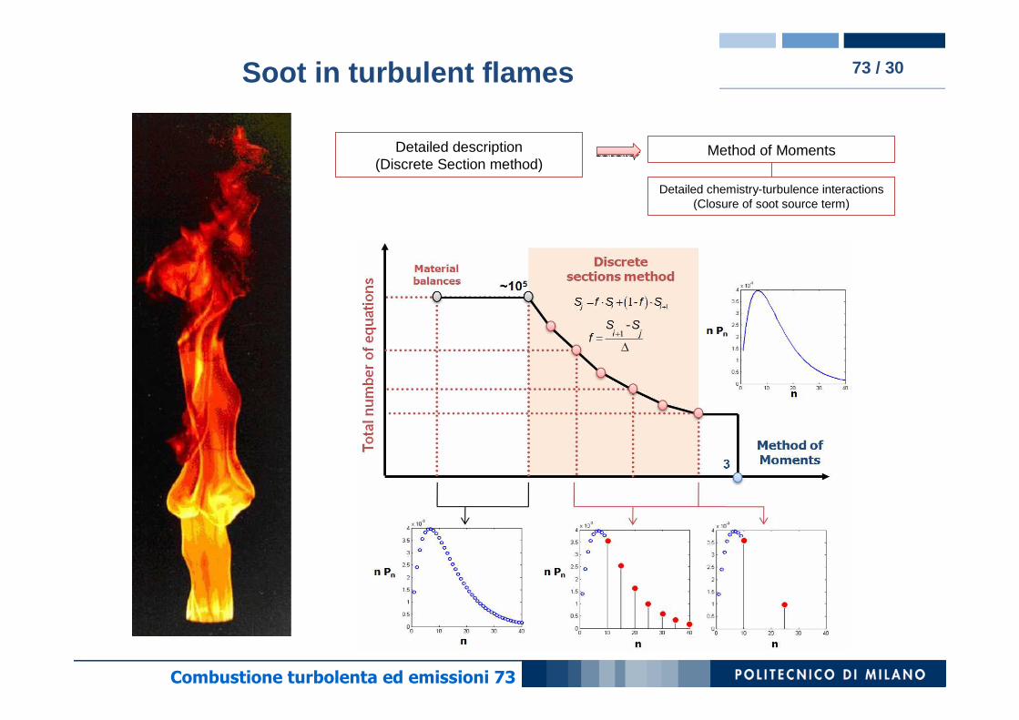
Large PAH and soot particles are divided in a finite number of sections or lumped components (BINs) which represent groups of species. The number of
conservation equations is just reduced to the number of sections.
Soot formation is described in the form of usual gas phase kinetics.
The discrete sectional method
BIN1: C24H12
PM = 300
BIN20: C12972032H1622016
PM > 150. E+6Dp ~ 30 nm
Soot formation: detailed mechanism 48 / 30
Adapted from: Bockhorn, H. , Soot Formation in Combustion:
Mechanisms and Models, Springer, Berlin (1994)

Combustione turbolenta ed emissioni 49
• Soot emissions from combustion devices have negative effects on human health
• Increasingly stringent limitations on soot emissions
=> need of reliable computational tools to predict soot formation in turbulent flames (inside CFD codes)
•Problems:
• two-way coupling between soot formation and thermal radiation
• complex chemistry to describe soot formation/oxidation
• importance of turbulence-chemistry interactions
Motivation: soot
PM: 40 µµµµg/m3PM: 40 µµµµg/m3PM: 8 µµµµg/m3PM: 8 µµµµg/m3

Combustione turbolenta ed emissioni 50
Soot formation in laminar flames can be successfully modeled using large detailed kinetic mechanism –> useful to understand the mechanism and develop/validate kinetic schemes.
• This analysis can help identifying the conditions that reduce soot formation
……in turbulent flames:
• The direct coupling of CFD codes and large kinetic mechanism is unfeasible due to the limited computational resources, especially considering the large grid used for complex geometries and industrial applications
• A complete decoupling (Pollutants Post-Processing, NOx) is not easily possible due to the effect of soot on thermal radiation.
Motivation: soot

Combustione turbolenta ed emissioni 51
Chemistry
Slow chemistry
Finite-ratechemistry
Fast chemistry
Fluiddynamics
Kolmogorov scale
Meanresidence time
ττττ(s)
103
100
102
101
10-1
10-4
10-2
10-3
10-5
10-8
10-6
10-7
10-9
NOx
Soot
Combustionprocess
The soot characteristic time is of the same order
of the fluid dynamics times.
Combustion process: Thermal field and species
can be successfully modeled using the flamelets
approach
Soot: strong interactions between fluid mixing and
chemical reactions
=>Specific approaches need to be used to model soot in turbulent flames.
Soot modeling in turbulent flames

Combustione turbolenta ed emissioni 52
• turbulent flames are successfully modeled using the flamelets approach and a presumed pdf of the mixture fraction (degree of mixing between fuel and air).
This allows to pre-process the kinetic calculations and store them in a library… computationally efficient but not possible for soot.
=> the approach used in this work
1) turbulent combustion is modeled using the flamelets approach (=> provides detailed temperature and composition fields T, CO, C2H2, CO2,OH… using detailed chemistry)
2) two additional balance equations are solved for soot number density and volume fraction:
semi-empirical (global) kinetic models for
nucleation, growth, aggregation, oxidation
Soot modeling in turbulent flames
Combustione turbolenta ed emissioni 53
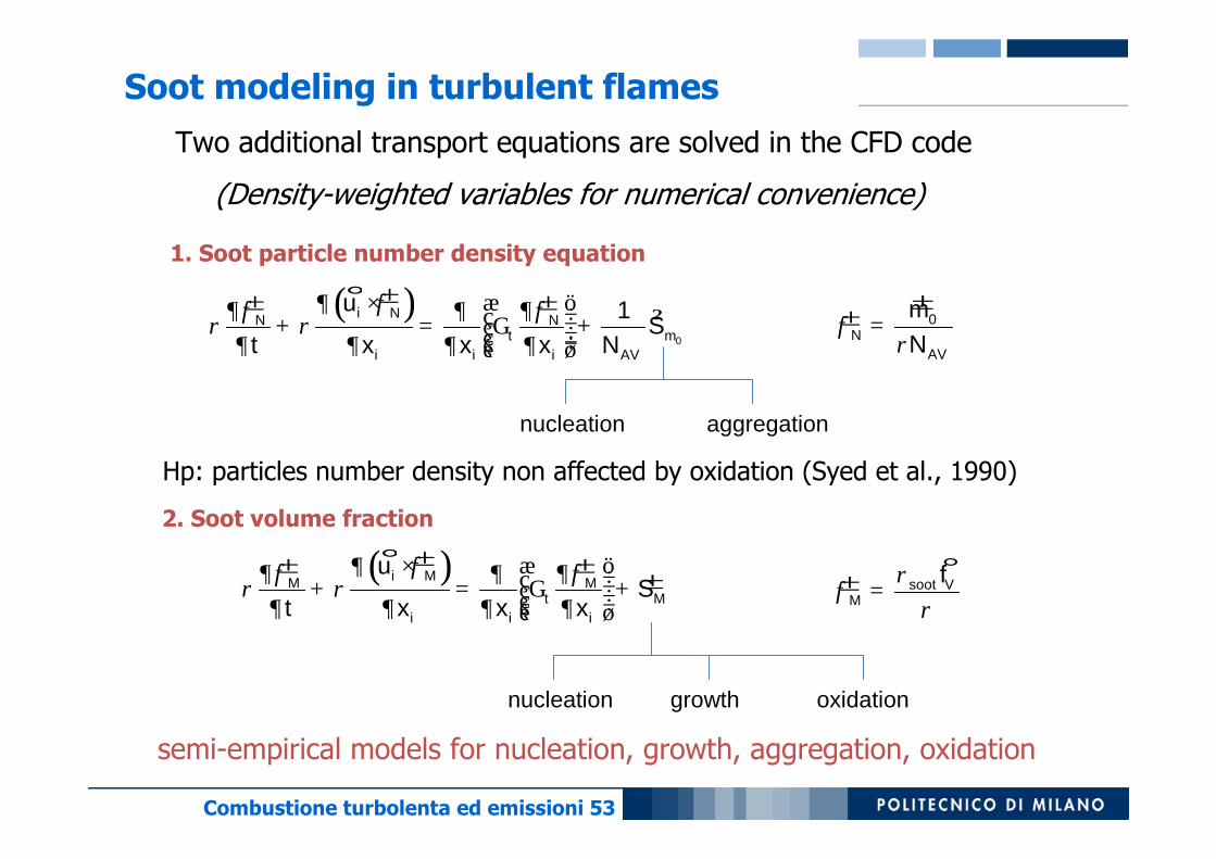
Two additional transport equations are solved in the CFD code
(Density-weighted variables for numerical convenience)
1. Soot particle number density equation
2. Soot volume fraction
± ° ±( ) ±²
ff fr r
æ ö¶ ׶ ¶¶ ÷ç ÷+ = G +ç ÷ç ÷÷ç¶ ¶ ¶ ¶è ø 0
1i NN Nt m
i i i AV
uS
t x x x N
± ° ±( ) ±±i MM M
t Mi i i
uS
t x x x
ff fr r
æ ö¶ ׶ ¶¶ ÷ç ÷+ = G +ç ÷ç ÷ç¶ ¶ ¶ ¶è ø
±±
fr
= 0N
AV
mN
±°r
fr
= soot VM
f
nucleation aggregation
nucleation growth oxidation
Hp: particles number density non affected by oxidation (Syed et al., 1990)
semi-empirical models for nucleation, growth, aggregation, oxidation
Soot modeling in turbulent flames
Combustione turbolenta ed emissioni 54
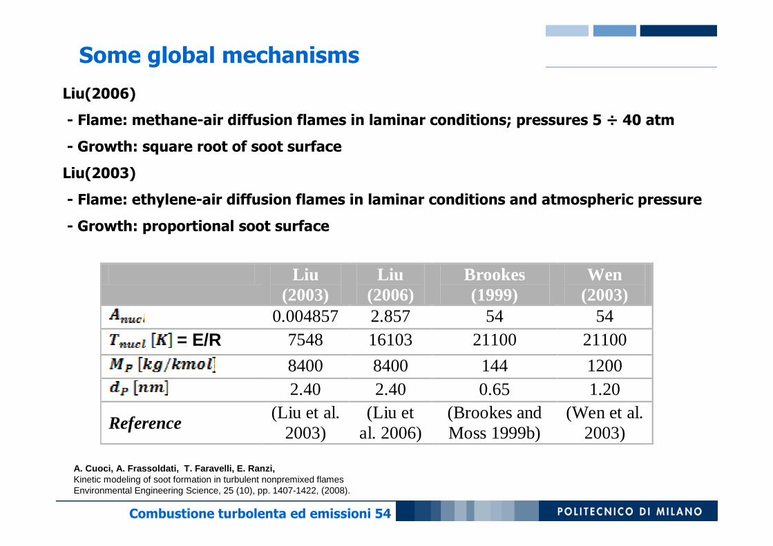
Liu(2006)
- Flame: methane-air diffusion flames in laminar conditions; pressures 5 ÷ 40 atm
- Growth: square root of soot surface
Liu(2003)
- Flame: ethylene-air diffusion flames in laminar conditions and atmospheric pressure
- Growth: proportional soot surface
Liu (2003)
Liu (2006)
Brookes (1999)
Wen (2003)
0.004857 2.857 54 54 = E/R 7548 16103 21100 21100
8400 8400 144 1200 2.40 2.40 0.65 1.20
Reference (Liu et al.
2003) (Liu et
al. 2006) (Brookes and Moss 1999b)
(Wen et al. 2003)
Some global mechanisms
A. Cuoci, A. Frassoldati, T. Faravelli, E. Ranzi,Kinetic modeling of soot formation in turbulent nonpremixed flamesEnvironmental Engineering Science, 25 (10), pp. 1407-1422, (2008).

Combustione turbolenta ed emissioni 55
Additional source term in in the energy equation
( )s ¥= - × × -4 44rad SQ a T T
( )( )1 2000soot soot va B f C Tr= × + -
2
1232.4m
Bkg
=
4 14.8 10C K- -= ×2 2 2 2S H O H O CO CO CO CO soota a p a p a p a= + + +
Ambient temperature ~300K
Absorption coefficient
Soot absorption coefficient
Sazhin1 (1994)
[1] S. S. Sazhin. An Approximation for the AbsorptionCoefficient of Soot in a Radiating Gas. Manuscript, FluentEurope, Ltd., 1994.
http://www.ca.sandia.gov/TNF/radiation.html
Soot radiation: asoot

Combustione turbolenta ed emissioni 56
The coupling between the flamelets library and radiation in a turbulent flame is achieved introducing a parameter called enthalpy defect1:
[1] Bray, K. N. C., and Peters, N. (1994). Turbulent Reacting Flows, P. A. Libby and F. A. Williams, eds., Academic Press, London, 78-84
( )f xé ù= - = - + -ë ûH AD OX FUEL OXH H H H H H
Using the laminar flamelet model the thermochemical state of a turbulent flame is completely determined by the mixture fraction ξ, the scalar dissipation rate χ and the enthalpy defect,
through the joint PDF P(ξ, χR, ΦΦΦΦH) :
° ( ) ( )1
0 0
, , , ,R H R H R HP d d dy y x c f x c f x c f+ ¥ + ¥
- ¥
= × × × ×ò ò ò
The single PDF’s are assumed to be statistically independent:
Scalar dissipation rate Log Normal
Distribution
Enthalpy defect Dirac
Delta
( ) ( ) ( ) ( )x c f x c f= × ×, ,R H R HP P P P
Mixture fraction β PDF
Sooting flames: non-adiabatic library
A. Cuoci, A. Frassoldati, T. Faravelli, E. Ranzi,Kinetic modeling of soot formation in turbulent nonpremixed flamesEnvironmental Engineering Science, 25 (10), pp. 1407-1422, (2008).

Combustione turbolenta ed emissioni 57
The mean enthalpy, used to obtain the enthalpy defect, is calculated from its conservation equation:
° ° °( ) °r r
æ ö¶ ׶ ¶ ¶ ÷ç ÷+ = G +ç ÷ç ÷ç¶ ¶ ¶ ¶è ø
i
t radi i i
u HH HQ
t x x x
FlameletLibrary
FlameletLibrary
Enthalpy Defect 1 (adiabatic)
Enthalpy Defect 1 (adiabatic)
Enthalpy Defect 2
Enthalpy Defect 2
Enthalpy Defect N
Enthalpy Defect N
Equilibrium Flamelet
Strain Rate 1
Strain Rate 2
Extinction Flamelet
Non-reacting Flamelet
The Flamelets library is pre-calculated and organized in shelves, each for a different value of Enthalpy Defect.
For each enthalpy defects several values of strain rate (represents the effect of turbulent flow on the flame)
(linear interpolation between the shelves)
Non-adiabatic Flamelets library
Combustione turbolenta ed emissioni 58
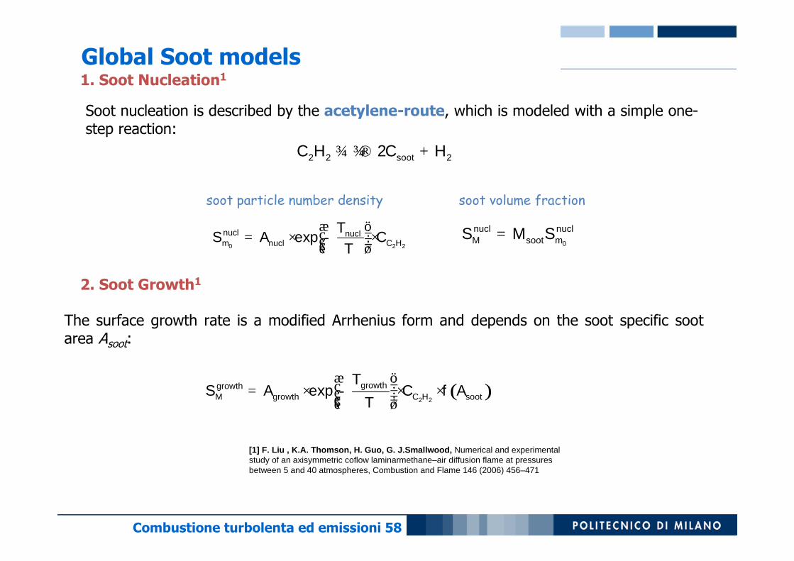
Soot nucleation is described by the acetylene-route, which is modeled with a simple one-step reaction:
1. Soot Nucleation1
soot particle number density soot volume fraction
2. Soot Growth1
The surface growth rate is a modified Arrhenius form and depends on the soot specific soot area Asoot:
¾ ¾® +2 2 22 sootC H C H
æ ö÷ç= × - ×÷ç ÷÷çè ø0 2 2expnucl nucl
m nucl C H
TS A C
T=
0
nucl nuclM soot mS M S
( )æ ö÷ç ÷= × - × ×ç ÷ç ÷çè ø 2 2
exp growthgrowthM growth C H soot
TS A C f A
T
[1] F. Liu , K.A. Thomson, H. Guo, G. J.Smallwood, Numerical and experimental study of an axisymmetric coflow laminarmethane–air diffusion flame at pressures between 5 and 40 atmospheres, Combustion and Flame 146 (2006) 456–471
Global Soot models
Combustione turbolenta ed emissioni 59
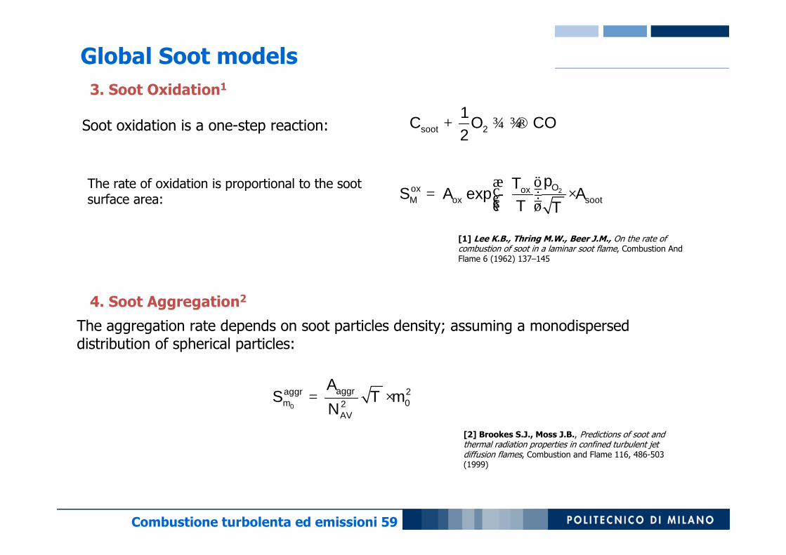
The rate of oxidation is proportional to the soot surface area:
Soot oxidation is a one-step reaction:
3. Soot Oxidation1
4. Soot Aggregation2
The aggregation rate depends on soot particles density; assuming a monodisperseddistribution of spherical particles:
+ ¾ ¾®2
12sootC O CO
2exp Oox oxM ox soot
pTS A A
T T
æ ö÷ç= - ×÷ç ÷çè ø
0
202
aggraggrm
AV
AS T m
N= ×
[1] Lee K.B., Thring M.W., Beer J.M., On the rate of combustion of soot in a laminar soot flame, Combustion And Flame 6 (1962) 137–145
[2] Brookes S.J., Moss J.B., Predictions of soot and thermal radiation properties in confined turbulent jet diffusion flames, Combustion and Flame 116, 486-503 (1999)
Global Soot models

Combustione turbolenta ed emissioni 60
This closure entirely ignores the effect of turbulence and formulates mean sourceterms from mean values alone.
=>In this case the joint-PDF simply becomes a combination of Dirac delta function centered on the mean value of each property:
( ) ( ) ±( ) ±( ) ±( ) °( )%x c f d x x d c c d f f d d= - × - × - × - × -0 0 0, , , ,R H V R R H H V VP m f m m f f
(I) Mean Properties Closure
This is the simplest approach and it has been largely used by many authors1,2,3,4.
[3] F. Liu, H. Guo, G. J.Smallwood, Gulder O., Numerical modelling of soot formation and oxidation in laminar coflow non-smoking and smoking ethylene diffusion flames, Combustion Theory and Modelling 7 (2003) 301–315
[1] Brookes S.J., Moss J.B., Predictions of soot and thermal radiationproperties in confined turbulent jet diffusion flames, Combustion and Flame 116, 486-503 (1999)
[2] Wen, Z., Yun, S., Thomson, M. J., and Lightstone, M. F. (2003). "Modeling soot formation in turbulent kerosene/air jet diffusion flames." Combustion and Flame, 135, 323-340
[4] Zucca, A., Marchisio, D. L., Barresi, A. A., and Fox, R. O. (2006). "Implementation of the population balance equation in CFD codes for modelling soot formation in turbulent flames." Chemical Engineering Science, 61, 87-95
Closure of the soot source term

Combustione turbolenta ed emissioni 61
(II) Uncorrelated Closure
The soot properties are assumed to be totally uncorrelated with the mixture fraction and the radiative heat loss and each other1,2.
Therefore the joint PDF has this form (Statistical Independence):
Unfortunately the individual PDFs for the soot particle number density and the soot fraction are unknown; therefore the PDF is further simplified:
( ) ( ) ±( ) °( )x c f x c f d d= × - × -0 0 0, , , , , ,R H V R H V VP m f P m m f f
( ) ( ) ( ) ( )x c f x c f= × ×0 0, , , , , ,R H V R H VP m f P P m P f
[1] Brookes S.J., Moss J.B. , Predictions of soot and thermalradiation properties in confined turbulent jet diffusion flames, Combustion and Flame 116, 486-503 (1999)
[2] Roditcheva, O. V., and Bai, X. S. (2001). "Pressure effect on soot formation in turbulent diffusion flames." Chemosphere, 42, 811-821
Closure of the soot source term
Combustione turbolenta ed emissioni 62
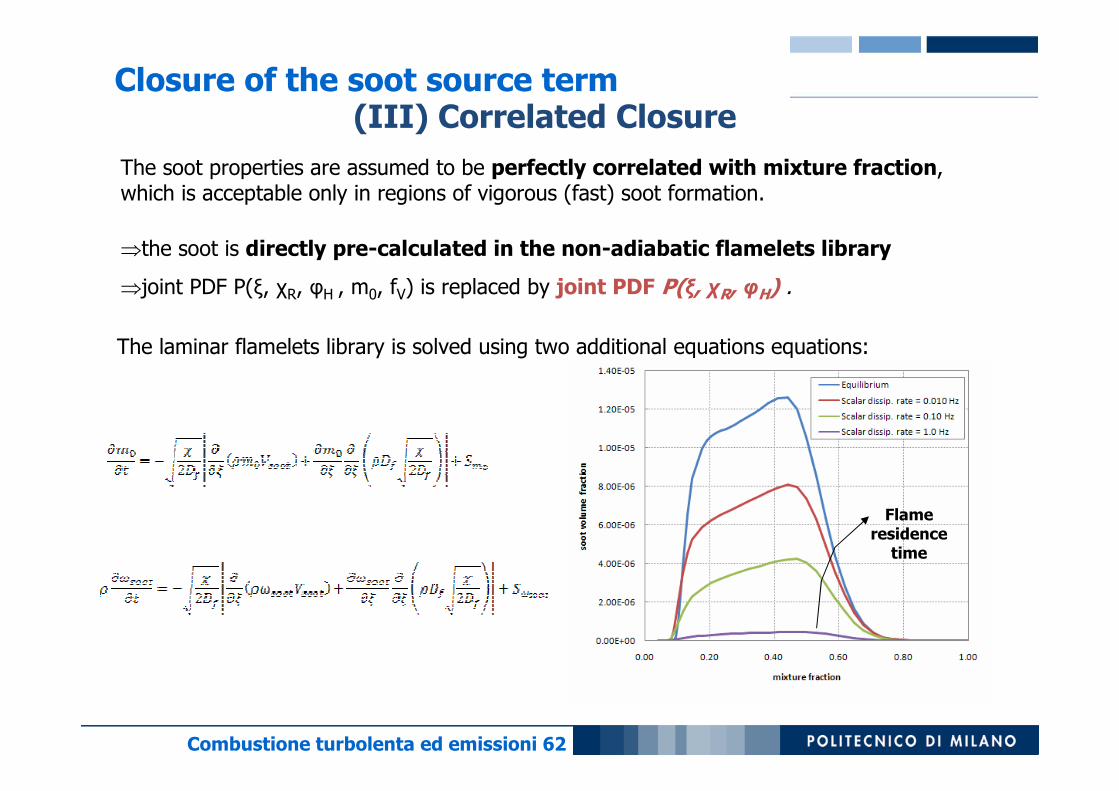
(III) Correlated Closure
The soot properties are assumed to be perfectly correlated with mixture fraction, which is acceptable only in regions of vigorous (fast) soot formation.
⇒the soot is directly pre-calculated in the non-adiabatic flamelets library
⇒joint PDF P(ξ, χR, φH , m0, fV) is replaced by joint PDF P(ξ, χR, φH) .
The laminar flamelets library is solved using two additional equations equations:
Flameresidence
time
Closure of the soot source term

Combustione turbolenta ed emissioni 63
Air
Ethylene
Air
Flame A: Ethylene turbulent jet flame (Kent & Honnery, 1987)
-Nozzle diameter = 3.00 mm
-Fuel velocity = 52 m/s
-Jet Reynolds number = 14660
-Turbulence: k-e model with correction for axisymmetric jets
-Radiative heat transfer: optically thin approximation (CO, CO2, H2O, Soot)
-Flamelets Model (POLIMI KINETIC SCHEME)
-Computational grid: axial-symmetric structured, non uniform, 120 x 60 cells
CFD Simulation (FLUENT 6.2)
Kent, Honnery , Soot and mixture fraction in turbulent diffusion flames, Combustion Science and Technology 54, 383-397 (1987)
Experimental data: jet flames

Combustione turbolenta ed emissioni 64
Flame B: Methane turbulent jet flame (Brookes & Moss, 1999)
-Nozzle diameter = 4.07 mm
-Fuel velocity = 20.3 m/s
-Jet Reynolds number = 5000
- Computational grid: structured, non uniform, 150 x 80 cells
CFD Simulation (FLUENT 6.2)
Brookes S.J., Moss J.B. , Predictions of soot and thermal radiation properties in confined turbulentjet diffusion flames, Combustion and Flame 116, 486-503 (1999)
Air
Methane
Air
Experimental data: jet flames

Combustione turbolenta ed emissioni 65
Temperature [K]
The CFD results refer to the simulation performed using the uncorrelated approach (II) for soot predictions.
Very similar results were obtained using the other closures.
Results flame A: Temperature

Combustione turbolenta ed emissioni 66
Soot Volume fraction
Comparison with experimental measurements
Soot volume fractionmean properties closure (I)
correlated closure (III)
uncorrelated closure (II)
(I)
(II)
(III)
(I)
(II)
(III)(II)
(III)
(I)
Results flame A: soot
Combustione turbolenta ed emissioni 67
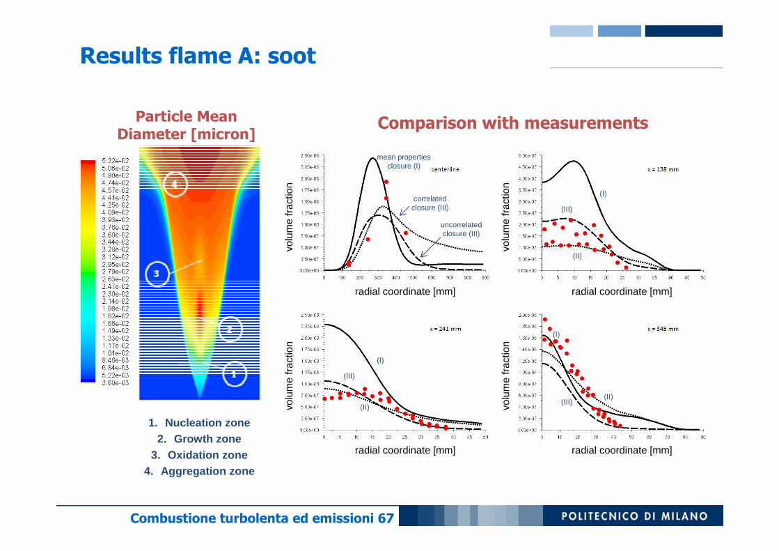
Particle Mean Diameter [micron]
Comparison with measurements
mean properties closure (I)
correlated closure (III)
uncorrelated closure (III)
(I)
(III)
(II)
(I)
(III)
(II)(III)
(II)
(I)
1. Nucleation zone2. Growth zone
3. Oxidation zone4. Aggregation zone
radial coordinate [mm]
volu
me
frac
tion
radial coordinate [mm]vo
lum
e fr
actio
n
radial coordinate [mm]
volu
me
frac
tion
radial coordinate [mm]
volu
me
frac
tion
Results flame A: soot
Combustione turbolenta ed emissioni 68
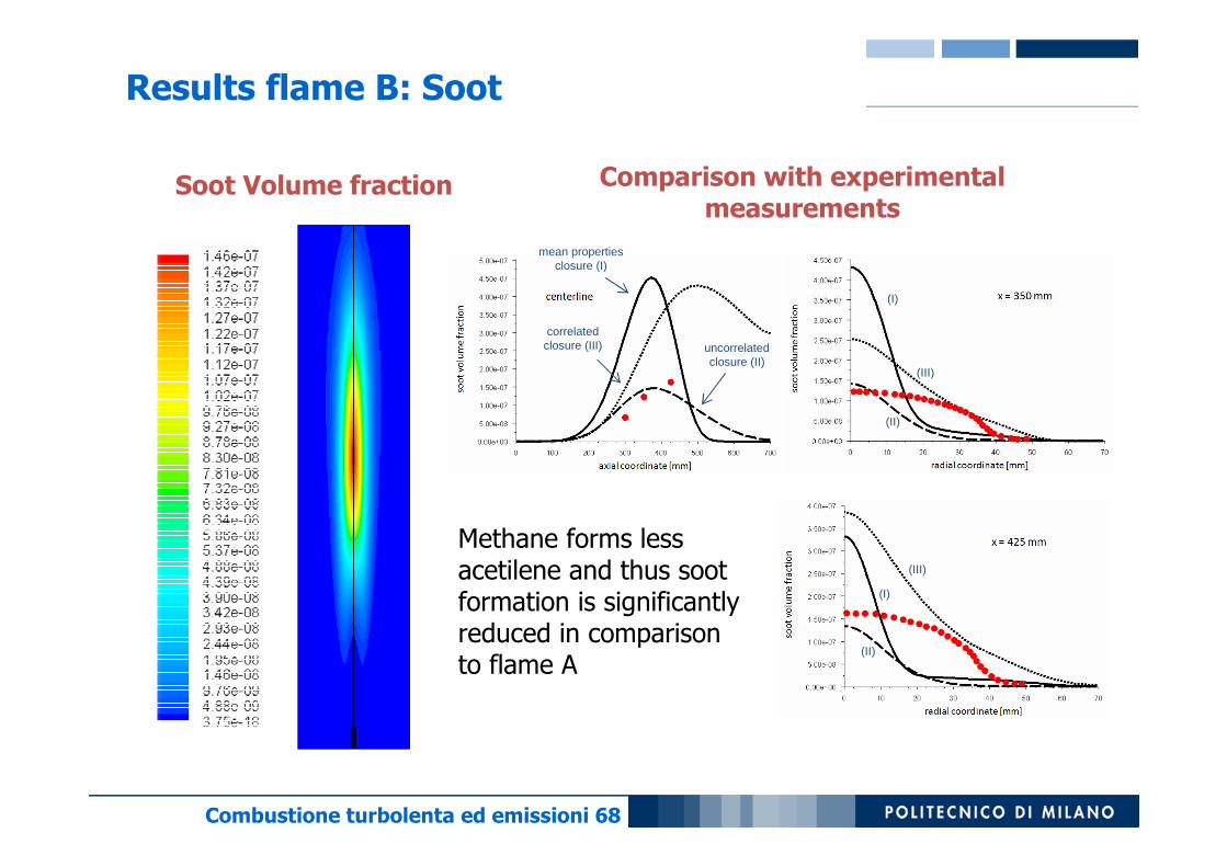
Soot Volume fraction
mean properties closure (I)
correlated closure (III) uncorrelated
closure (II)
(I)
(III)
(II)
Comparison with experimental measurements
(I)
(III)
(II)
Methane forms less acetilene and thus soot formation is significantly reduced in comparison to flame A
Results flame B: Soot
Combustione turbolenta ed emissioni 69
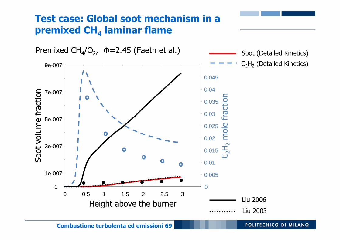
Premixed CH4/O2, Φ=2.45 (Faeth et al.)
0
1e-007
3e-007
5e-007
7e-007
9e-007
0 0.5 1 1.5 2 2.5 3
Soot
volu
me fra
ctio
n
Height above the burner
0.005
0.01
0.015
0.02
0.025
0.03
0.035
0.04
0.045
0
C2H
2m
ole
fra
ctio
n
Soot (Detailed Kinetics)
Liu 2006
Liu 2003
C2H2 (Detailed Kinetics)
Test case: Global soot mechanism in a premixed CH4 laminar flame

Combustione turbolenta ed emissioni 70
Soot (Detailed Kinetics)
Liu 2006
Liu 2003
C2H2 (Detailed Kinetics)Premixed Benzene/O2/N2 (Ciajolo)
Soot
conce
ntr
ation
[g/c
m3]
Height above the burner
0
2e-007
4e-007
6e-007
8e-007
1e-006
1.2e-006
0 0.2 0.4 0.6 0.8 1 1.2 1.4 1.60
0.002
0.004
0.006
0.008
0.010
0.012
0.014
C2H
2m
ole
fra
ctio
n
Test case: Global soot mechanism in a premixed Benzene laminar flame

Combustione turbolenta ed emissioni 71
T. Faravelli, A. Frassoldati and E. RanziKinetic Modeling of Mutual Interactions in NO-Hydrocarbon Low Temperature Oxidation Combustion and Flame, 132/1-2 pp 188 - 207 (2003)
A. Frassoldati, T. Faravelli and E. RanziKinetic Modeling of Mutual Interactions in NO-Hydrocarbon High Temperature OxidationCombustion and Flame 135, pp. 97-112, (2003)
A. Frassoldati, S. Frigerio, E. Colombo, F. Inzoli, T. FaravelliDetermination of NOx emissions from strong swirling confined flames with an integrated CFD-based procedureChem. Eng. Sci. 60, pp. 2851-2869, (2005).
E. Ranzi, A. Frassoldati, S. Granata, T. FaravelliWide-Range Kinetic Modeling Study of the Pyrolysis, Partial Oxidation, and Combustion of Heavy n-AlkanesInd. Eng. Chem. Res. (2005) 44(14), 5170-5183
S. Granata, A. Frassoldati, T. Faravelli, E. Ranzi, S. Humer, K. SeshadriPolycyclic Aromatic Hydrocarbons and Soot Particle Formation in Liquid Fuel CombustionChem. Engng. Transactions Vol. 10 pp. 275-280 AAAS AIDIC Milano 2006
A. Cuoci, A. Frassoldati, G. Buzzi Ferraris, T. Fara velli, E. Ranzi, Ignition, Combustion and Flame Structure of Carbon Monoxide/Hydrogen Mixtures. Note 2: fluid Dynamics and Kinetics Aspects of Syngas CombustionInt. J. of Hydrogen Energy, 32: 3486-3500 (2007)
A. Cuoci, A. Frassoldati, T. Faravelli, E. Ranzi,Kinetic modeling of soot formation in turbulent nonpremixed flamesEnvironmental Engineering Science, 25 (10), pp. 1407-1422, (2008).
A. Frassoldati, A. Cuoci, T. Faravelli, E. Ranzi, D . Astesiano, M. Valenza, P. Sharma,Experimental and modelling study of low-NOx industrial burnersMPT Metallurgical Plant and Technology International, 31 (6), pp. 44-46, (2008).
References
Combustione turbolenta ed emissioni 72
ReferencesA. Cuoci, A. Frassoldati, T. Faravelli, E. Ranzi, Frequency response of counter flow diffusion flames to strain rate harmonic oscillations,Combustion Science and Technology, 180 (2008), pp. 767-784
A. Frassoldati, A. Cuoci, T. Faravelli, E. Ranzi, S . Colantuoni, P. Di Martino, G. Cinque,Experimental and modeling study of a low NOx combustor for aero-engine turbofanCombustion Science and Technology, 181 (3), pp. 483-495, (2009).
A. Frassoldati, A. Cuoci, T. Faravelli, E. Ranzi, G . Buzzi Ferraris,Robust and efficient numerical methods for the prediction of pollutants using detailed kinetics and fluid dynamicsComputer Aided Chemical Engineering, 26, pp. 707-711 (2009).
A. Cuoci, A. Frassoldati, T. Faravelli, E. Ranzi,Formation of soot and nitrogen oxides in unsteady counterflow diffusion flamesCombustion and Flame, 156 (10), pp. 2010-2022, (2009)
D. Manca, G. Buzzi Ferraris, A. Cuoci, A. Frassoldat i,The solution of very large non-linear algebraic systemsComputers and Chemical Engineering, 33 (10), pp. 1727-1734 (2009)
A. Parente, A. Cuoci, C. Galletti, A. Frassoldati, T. Faravelli, L. Tognotti, NO formation in flameless combustion: comparison of different modeling approaches, paper number 810.144, 4th European Combustion Meeting, Vienna, Austria, 14 - 17 April 2009.
A. Frassoldati, P. Sharma, A. Cuoci, T. Faravelli, E. Ranzi, Kinetic and Fluid Dynamics Modelling of a Methane/Hydrogen Jet Flames in Diluted Coflow, paper number 810.145, 4th European Combustion Meeting, Vienna, Austria, 14 - 17 April 2009.
A. Frassoldati, A. Cuoci, T. Faravelli, E. Ranzi, S . Colantuoni, P. Di Martino, G. Cinque, M. Kern, S. Marinov, N. Zarzalis, Fluid dynamics and detailed kinetic modeling of pollutant emissions from lean combustion systems, Sixth Mediterranean Combustion Symposium, Porticcio – Ajaccio, Corsica, France, June 7-11, 2009
Combustione turbolenta ed emissioni 73
Soot in turbulent flames
Detailed description (Discrete Section method)
Method of Moments
Detailed chemistry-turbulence interactions(Closure of soot source term)
73 / 30
Combustione turbolenta ed emissioni 74
( )0
1i NN Nt m
i i i AV
uS
t x x x N
φφ φρ ρ∂ ⋅ ∂ ∂∂+ = Γ + ∂ ∂ ∂ ∂
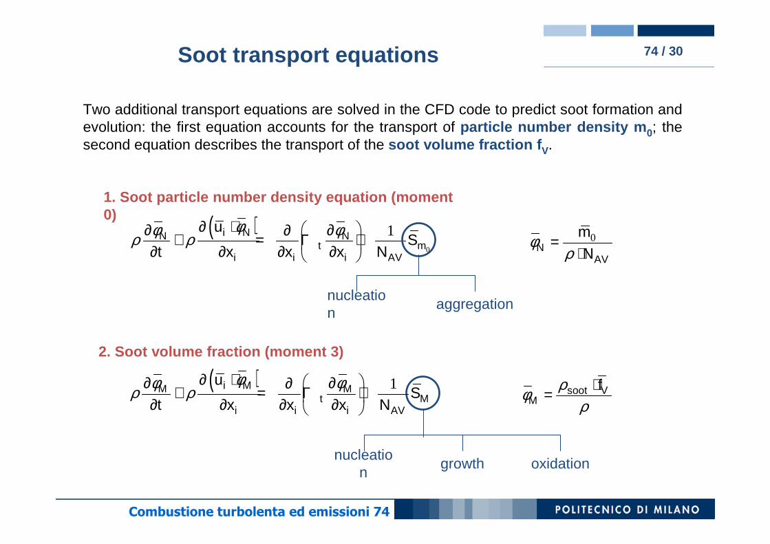
Two additional transport equations are solved in the CFD code to predict soot formation and evolution: the first equation accounts for the transport of particle number density m0; the second equation describes the transport of the soot volume fraction fV.
1. Soot particle number density equation (moment 0)
2. Soot volume fraction (moment 3)
nucleation
aggregation
nucleation
growth oxidation
Soot transport equations 74 / 30
( ) 1i MM Mt M
i i i AV
uS
t x x x N
φφ φρ ρ∂ ⋅ ∂ ∂∂+ = Γ + ∂ ∂ ∂ ∂
0N
AV
mN
φρ
=⋅
soot VM
fρφρ
⋅=

Combustione turbolenta ed emissioni 75
Turbulence model
Scalar dissipationrate
Soot Library
Soot source term: m0 equation
Coupling between CFD and soot library 75 / 30
RANS code
mass
momentum
energy
species
Turbulent kinetic energy
Dissipation rate of turbulent kinetic energy
Soot source term: fv equation
Soot Transport Equation- m0 equation
- fv equation
A. Cuoci, A. Frassoldati, T. Faravelli, E. Ranzi, “Kinetic Modeling of Soot Formation in Turbulent Flames”, Environmental Engineering Science, 25(10):1407-1422, 2008
( )2'', ,st stχ χ κ ε ξ=
Combustione turbolenta ed emissioni 76
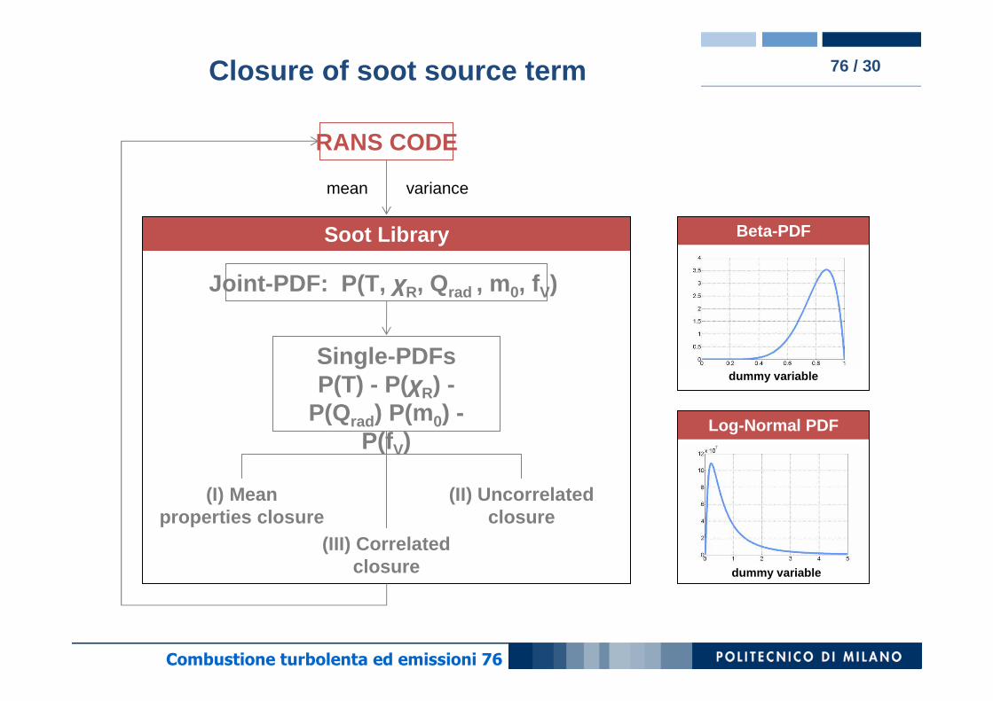
Closure of soot source term 76 / 30
Soot Library
RANS CODE
Single-PDFsP(T) - P(χR) -
P(Qrad) P(m0) -P(fV)
(I) Mean properties closure
(II) Uncorrelated closure
(III) Correlated closure
Joint-PDF: P(T, χR, Qrad , m0, fV)
mean variance
Log-Normal PDF
dummy variable
Beta-PDF
dummy variable

Combustione turbolenta ed emissioni 77
Additional
Combustione turbolenta ed emissioni 78
The application example: FLOX(R)
burner
0 2000 4000 6000 8000
0
2000
4000
6000
8000
Cell index
Cel
lind
ex
0 2000 4000 6000 8000
0
2000
4000
6000
8000
Cell index
Cel
lind
ex
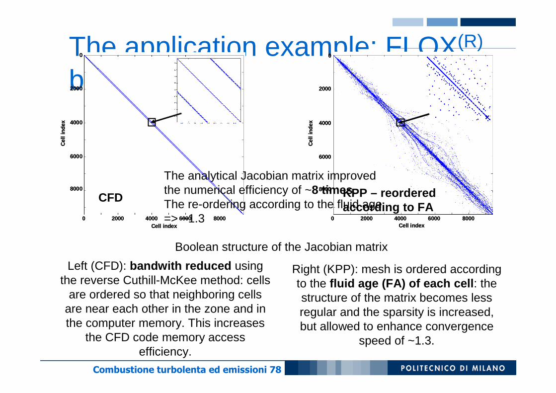
Boolean structure of the Jacobian matrix
Left (CFD): bandwith reduced usingthe reverse Cuthill-McKee method: cells
are ordered so that neighboring cellsare near each other in the zone and in the computer memory. This increases
the CFD code memory accessefficiency.
Right (KPP): mesh is ordered accordingto the fluid age (FA) of each cell : the structure of the matrix becomes lessregular and the sparsity is increased, but allowed to enhance convergence
speed of ~1.3.
0 2000 4000 6000 8000
0
2000
4000
6000
8000
Cell index
Cel
lind
ex
0 2000 4000 6000 8000
0
2000
4000
6000
8000
Cell index
Cel
lind
ex
CFD KPP – reorderedaccording to FA
The analytical Jacobian matrix improved the numerical efficiency of ~8 times . The re-ordering according to the fluid age => ~1.3

Combustione turbolenta ed emissioni 79
Semplificazione problema
Cinetica complessa
Fluidodinamica complessa
Problema intrattabile
Cinetica semplice
-- previsione meno …accurata
-- modelli tarati sul …singolo problema
Fluidodinamica semplice
-- soluzione semplice
-- misure sperimentali di …laboratorio

Combustione turbolenta ed emissioni 80
Struttura delle fiamme
• Fiamme laminari diffusive contrapposte
Combustione turbolenta ed emissioni 81
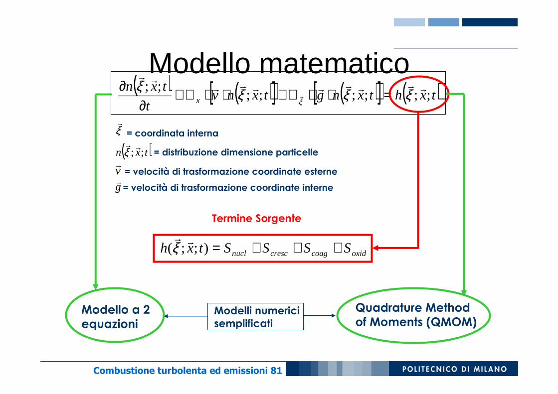
Modello matematico( ) ( )[ ] ( )[ ] ( )txhtxngtxnv
t
txnx ;;;;;;
;; rrrrrrrrrr
r ξξξξξ =⋅⋅∇+⋅⋅∇+
∂∂
ξr
= coordinata interna
( )txn ;;rr
ξ = distribuzione dimensione particelle
vr= velocità di trasformazione coordinate esterne
gr= velocità di trasformazione coordinate interne
Modello a 2 equazioni
Quadrature Methodof Moments (QMOM)
Modelli numerici semplificati
oxidcoagcrescnucl SSSStxh +++=);;(rr
ξ
Termine Sorgente
Combustione turbolenta ed emissioni 82
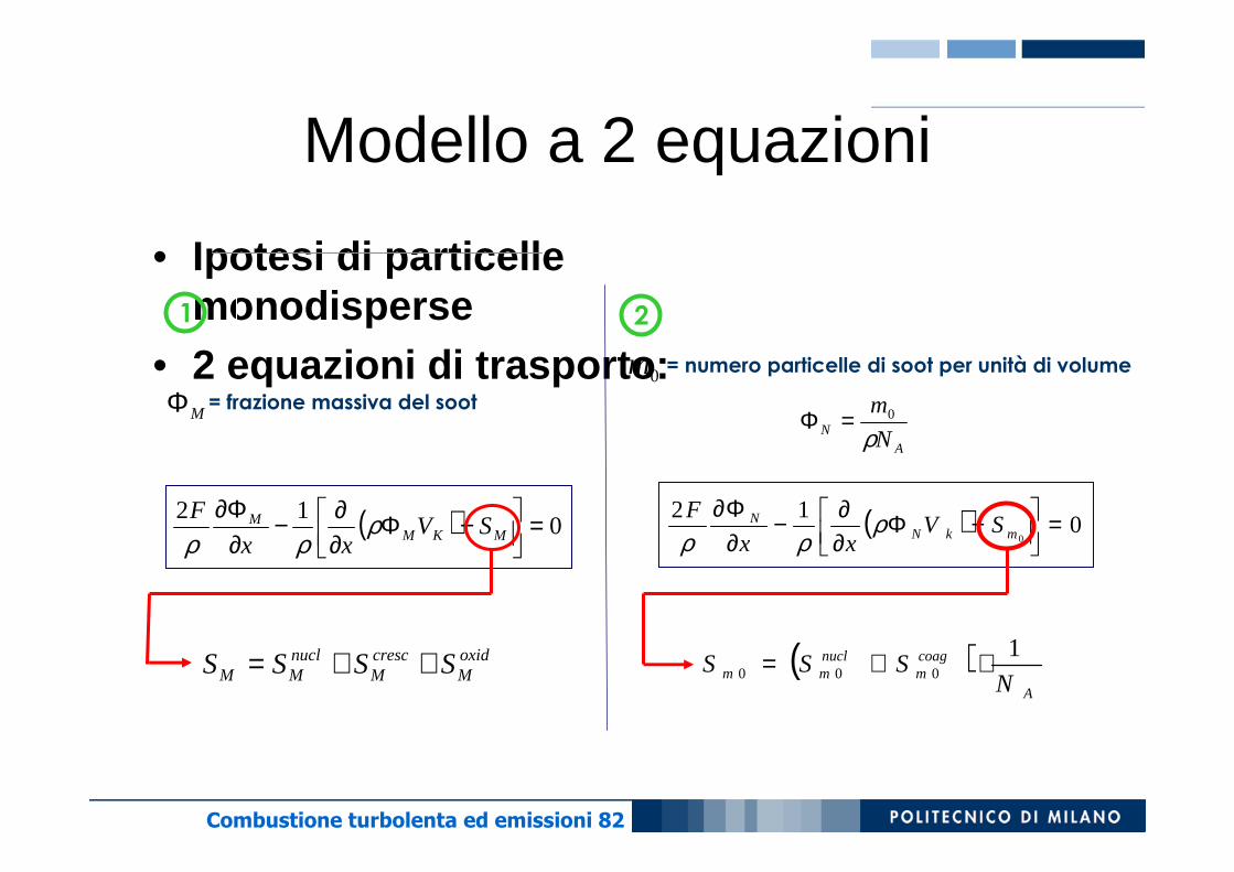
Modello a 2 equazioni
• Ipotesi di particelle monodisperse
• 2 equazioni di trasporto:1
MΦ = frazione massiva del soot
( ) 012 =
−Φ∂∂−
∂Φ∂
MKMM SV
xx
F ρρρ
oxidM
crescM
nuclMM SSSS ++=
2
0m = numero particelle di soot per unità di volume
AN N
m
ρ0=Φ
( ) 012
0=
−Φ∂∂−
∂Φ∂
mkNN SV
xx
F ρρρ
( )A
coagm
nuclmm N
SSS1
000 ⋅+=

Combustione turbolenta ed emissioni 83
Quadrature Method of Moments
La distribuzione della dimensione di particelle è approssimata da una combinazione lineare di delta di Dirac
( ) ( )1 1
( ) ( )NN
ij
f w t tαα
ξ δ ξ ξ= =
≈ ⋅ −∑ ∏( )tiξ = ascisse ( )twα = pesi
x
w Original particle sizedistribution
x
wQMOM (N=2)
2N incognite:
-- N ascisse
-- N pesi
Le N ascisse e gli N pesi vengono calcolati imponendo che i momenti della distribuzione discreta siano uguali a quelli delladistribuzione continua.
1
NQMOM k
k km m wα αα
ξ=
= = ⋅∑ 0...2 1k N= −con
( ) 012 )( =
−∂∂+
∂∂ N
kkkk SVm
xx
mF ρρρ
con k=0,…, 1−N