combining the modified discrete element method with … · · 2017-02-07combining the modified...
TRANSCRIPT

COMBINING THE MODIFIED DISCRETE ELEMENT METHOD
WITH THE VIRTUAL ELEMENT METHOD FOR FRACTURING
OF POROUS MEDIA.
HALVOR MØLL NILSEN, IDAR LARSEN, AND XAVIER RAYNAUD
Abstract. Simulation of fracturing processes in porous rocks can be dividedinto two main branches: (i) modeling the rock as a continuum which is en-
hanced with special features to account for fractures, or (ii) modeling the rock
by a discrete (or discontinuous) approach that describes the material directlyas a collection of separate blocks or particles, e.g., as in the discrete element
method (DEM). In the modified discrete element (MDEM) method, the effec-
tive forces between virtual particles are modified in all regions, without failingelements, so that they reproduce the discretization of a first order finite element
method (FEM) for linear elasticity. This provides an expression of the virtual
forces in terms of general Hook’s macro-parameters. Previously, MDEM hasbeen formulated through an analogy with linear elements for FEM. We show
the connection between MDEM and the virtual element method (VEM), whichis a generalization of FEM to polyhedral grids. Unlike standard FEM, which
computes strain-states in a reference space, MDEM and VEM compute stress-
states directly in real space. This connection leads us to a new derivation of theMDEM method. Moreover, it gives the basis for coupling (M)DEM to domain
with linear elasticity described by polyhedral grids, which makes it easier to
apply realistic boundary conditions in hydraulic-fracturing simulations. Thisapproach also makes it possible to combine fine-scale (M)DEM behavior near
the fracturing region with linear elasticity on complex reservoir grids in the
far-field region without regridding. To demonstrate the simulation of hydraulicfracturing, the coupled (M)DEM-VEM method is implemented using the Mat-
lab Reservoir Simulation Toolbox (MRST) and linked to an industry-standard
reservoir simulator. Similar approaches have been presented previously usingstandard FEM, but due to the similarities in the approaches of VEM and
MDEM, our work is a more uniform approach and extends these previousworks to general polyhedral grids for the non-fracturing domain.
1
arX
iv:1
702.
0155
2v1
[m
ath.
NA
] 6
Feb
201
7

2 HALVOR MØLL NILSEN, IDAR LARSEN, AND XAVIER RAYNAUD
1. Introduction
Effective control of flows in geological formations is a key factor for exploiting re-sources that are highly important for the society, such as ground water, geothermalenergy, geological storage of CO2, high quality fossil fuel (gas and oil) and poten-tially large scale storage of energy in terms or heat or gas. Today 60% of the worldenergy consumption is based on oil and natural gas resources [22]. In addition 19%is based on coal which needs large scale CO2 storage to be safely exploited withoutlarge scale impact on climate [33]. Geothermal energy is an important source ofgreen energy, which would be even more valuable in the future as the supply offossil fuel is expected to decrease. Gas storage is today an integrated part of theenergy supply and provides reliable large scale storage of energy. It enables to bothattenuate the volatility of energy prices and ensure energy security.
The use of all of the above resources will benefit from a reliable control of theflow properties around the wells that are used to exploit them. Increased injectivityis particularly important for exploiting resources in tight formation or where highflow rates are required. For enhanced geothermal applications, rock fracturing is aprerequisite for economical exploitation. For CO2 injection, where large volumes offluid have to be injected, high injectivity limits the increase in pressure near the welland simplifies the operation. Tight formations contain much of the hydrocarbonreserves. The exploitation of these formations has been a driving force for thetechnology of fracking, which is a more drastic well stimulation than the traditionalones. When increasing the injectivity in a well, it is of vital importance to beable to predict and control fracturing to avoid unwanted fractures or even inducedseismic events, which may cause environmental damage as well as the disruptionof operations. The key for enabling high injectivity is to induce and control thefracturing process using the coupling between fluid flow, heat and rock mechanics.The failure of the rock and the propagation of fractures depend on both global andlocal effects, through the stress distribution which is intrinsically global and failurecriterias which are local. It is therefore important to have flexible simulation toolsthat are able to cover both large scale features with complex geometry and includespecific fracture dynamics where the fracturing processes occur.
Numerical methods for simulating fracturing can typically be classified eitheras continuum or discontinuum based methods [23]. The modeling of fracturing inbrittle materials like rock is particularly difficult. It is determined by the stress fieldin the vicinity of the fracture tip. As [15] showed, failures happen when the globalenergy release is larger than the energy required by the fracturing process. Thefirst depends on the global stress field while the latter is associated with the energyneeded at small scale to create a fracture. For brittle materials where the failurehappens at very small scales, linear elasticity governs the behavior in most of thedomain but the solution of linear elasticity in the presence of fractures is singularnear the fracture tip (see [25] for a general description). This introduces challengesfor numerical calculations and often results in artificial grid dependence of thesimulated dynamics. From a physical point of view, such effects are removed whenplasticity is introduced, however the length scale of this region may be prohibitivelysmall to be resolved numerically on the original model. Several techniques havebeen introduced to incorporate the singularity at the fracture tip into the numericalcalculations explicitly, for example specific tip elements in the finite element FEMmethod. In general, the methods using global energy arguments are less sensitive

COMBINING MDEM AND VEM FOR FRACTURING MODELING 3
to the choice of numerical methods than those that use estimates of the strength ofthe singularity [25]. In the case of the fracturing of natural rock, the uncertainty inthe model is large, small scale heterogeneities are important and several differentfracturing mechanisms complicate the structure. Discrete modeling techniques havebeen very successful in this area [28], in particular if complex behaviors should besimulated.
An essential component to model fracturing is therefore the ability to accountin a flexible manner for both large and small scale behaviors. This is reflected inthe widespread use of tools based on analytic models for hydraulic fracturing (for areview see [26]). However, it becomes a challenge to incorporate interaction of frac-tures and fine-scale features into those simulation tools. Because of their simplicityand flexibility for incorporating different fracturing mechanisms, discrete elementmethods (DEM), also called in their explicit variants, distinct element methods,have been one of the main techniques used for hydraulic fracturing in commercialsimulators. Those methods exploit the ability of easily modifying the interactionsand connections between the discrete particles or elements. For continuum models,such behavior is more difficult to account for. However, the parameters in the DEMmodel are not directly related to physical macro-scale parameters and there are re-strictions on the range of the parameters that can be simulated. In particular, [4]showed that only Poisson’s ratios (in plain stress) smaller than 1/3 can be consid-ered. The modified discrete element method (MDEM) was introduced to get rid ofthis restriction and gives also easier relationships between the macro parameters inthe linear elastic domain, while keeping the advantages of DEM in the treatmentof fracture. In this work, we show the connection between MDEM and the recentdevelopment of Virtual Element Methods (VEM). Such approach provides a simplederivation of the MDEM framework, and also highlight the discrepancy of the orig-inal DEM model from linear elasticity. The linear version of the VEM methods forelasticity can be used to extend first-order FEM on simplex grids, which was thebasis of the MDEM method, to general polyhedral grids. We use the fact that bothDEM, MDEM and VEM share the same degrees of freedom in the case of simplexgrids to derive smooth couplings between these methods. A similar approach hasbeen followed for coupling FEM with DEM previously [34, 38]. The introductionof VEM opens the possibility for flexible gridding on general polyhedral grids inthe far-field region while keeping the DEM/MDEM flexibility in the near fracturedomains. Geological formations are typically the result of deposition and erosionprocesses, which lead to layered structures and faults. Geometrical models usingpolyhedral grids, such as Corner Point Grid [36], Skua Grid [16] and Cut-Cell [29]are natural in this context and correspond to grids used in the industry of flow mod-eling in reservoirs. Our proposed method therefore may simplify the incorporationof fracture simulation in realistic subsurface applications.
2. Methods
We study the methods for the standard equations of linear elasticity given by
(1)
∇ · σ = f ,
ε =1
2(∇+∇T )u,
σ = Cε,

4 HALVOR MØLL NILSEN, IDAR LARSEN, AND XAVIER RAYNAUD
where σ is the Cauchy stress tensor, ε the infinitesimal strain tensor and u the dis-placement field. The linear operator C is the fourth-order Cauchy stiffness tensor.In Kelvin notation [19], a three-dimensional symmetric tensor εij is representedas an element of R6 with components
[ε11, ε22, ε33,√
2ε23,√
2ε13,√
2ε12]T
while a two-dimensional symmetric tensor is represented by a vector in R3 given by[ε11, ε22,
√2ε12]T . Using this notation C can be represented by a 6× 6 matrix and
inner products of tensors correspond to the normal inner-product of vectors. Forisotropic materials, we have the constitutive equations
(2) σ = 2µε+ λ tr(ε) I .
where µ and λ denote the Lame constants. The elastic energy density is given by12σ : ε where we use the standard scalar product for matrices defined as
α : β = tr(αTβ) =
3∑i,j=1
αi,jβi,j ,
for any two matrices α, β ∈ R3×3.
2.1. Discete element method. Discrete element methods consist of modelingthe mechanical behaviour of a continuum material by representing it as a set ofparticles, or discrete elements. The forces in the material are then modeled asinteraction forces between the particles. There are several variants of the discreteelement method [28]. Here we will use the simple version introduced in [4] wherethe particles are discs in 2D and spheres in 3D. We will also restrict the treatmentto the linear case to compare with linear elasticity, but this is not a restriction ofthe method. For more in-depth presentation of different variants see [28] or [10]and the references therein.
The starting point of the DEM methods has its background in the description ofgranular media. This has a long history starting from the description of the contactforce by Hertz and [30]. In this field an important question was to study how theeffective elastic modulus of the bulk was related to the microscopic description[12, 40]. In DEM the basic ideas is to use a microscopic description to simulate thebehavior of the bulk modulus.
For a complete relation between general DEM method and linear elasticity usingshear forces, it is necessary to introduce the material laws for micropolar mate-rials, see [4]. This introduces an extra variable associated with local rotation, asillustrated in Figure 1. For an isotropic micropolar media the strain stress relationis
(3) σ = 2µε+ λ tr(ε) I +κ(τ − φ)
where the extra variable φ describe the local rotation and τ represent the asym-metric part of the strain tensor, i.e, rigid body rotations. In terms of displacementsit can be written
(4) τ =1
2(∇u−∇Tu).

COMBINING MDEM AND VEM FOR FRACTURING MODELING 5
~Fs ~Fn
(~ri, θi)
(~rj , θj)(~rk, θk)
(a) DEM
di,j
fi,jσ
ε
~ri
~rj~rk
(b) MDEM
Figure 1. This show the fundamental quantities used in DEM (a)and MDEM (b). The unit colored in red for MDEM defines thearea which is used to calculated the one sided forces.
The state variable are the displacement u and the local rotation φ and the totalelastic energy is given by
(5) E =
∫Ω
(µε : ε+λ
2tr(ε)2 +
κ
2(τ − φ) : (τ − φ)) dx.
By computing the variation of E,
δE =
∫Ω
(∇ · (2µε+ λ tr(ε) I +κ(τ − φ)) · δu) dx+
∫Ω
κ(τ − φ) : δφ dx,
we obtain the governing equations of the system, that is, the linear momentumconservation equation,
(6a) ∇ · (2µε+ λ tr(ε) I +κ(τ − φ)) = 0
and the angular momentum conservation equation
(6b) τ − φ = 0.
We will use the expression of the stress given by (3) to compare with the DEMmodel which include local rotations. Let us consider two particles p1 and p2 whichare connected through a contact denoted m. For a particle pi, i = 1, 2, we denoteby Xpi the position of the particle. The degrees of freedom of the system are thedisplacement Upi and the microrotation θpi for each particle pi. Furthermore weset
∆Xm = Xp2 −Xp1 , ∆Um = Up2 − Up1 , Im =∆Xm
|∆Xm| .
We introduce also the distance between the particles, dm = |∆Xm|. We use thecross-product to represent the action of a rotation so that the rotation given by avector θ is the mapping given by X → θ ×X. Our description of DEM follows [4]with slight differences in the notation. We introduce the normal and shear forces,
(7) Fmn = kn∆Umn Fms = ks∆Ums .
For a given contact m the relative shear and normal displacement are given by
∆Umn = (∆Um · Im)Im,
∆Ums = ∆Um −∆Umn − θm ×∆Xm,
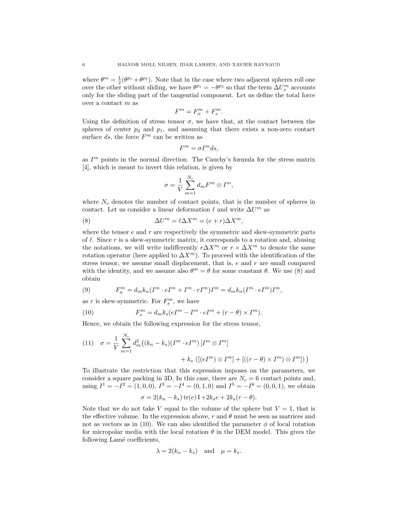
6 HALVOR MØLL NILSEN, IDAR LARSEN, AND XAVIER RAYNAUD
where θm = 12 (θp1 +θp2). Note that in the case where two adjacent spheres roll one
over the other without sliding, we have θp1 = −θp2 so that the term ∆Ums accountsonly for the sliding part of the tangential component. Let us define the total forceover a contact m as
Fm = Fmn + Fms .
Using the definition of stress tensor σ, we have that, at the contact between thespheres of center p2 and p1, and assuming that there exists a non-zero contactsurface ds, the force Fm can be written as
Fm = σImds,
as Im points in the normal direction. The Cauchy’s formula for the stress matrix[4], which is meant to invert this relation, is given by
σ =1
V
Nc∑m=1
dmFm ⊗ Im,
where Nc denotes the number of contact points, that is the number of spheres incontact. Let us consider a linear deformation ` and write ∆Um as
(8) ∆Um = `∆Xm = (e+ r)∆Xm,
where the tensor e and r are respectively the symmetric and skew-symmetric partsof `. Since r is a skew-symmetric matrix, it corresponds to a rotation and, abusingthe notations, we will write indifferently r∆Xm or r × ∆Xm to denote the samerotation operator (here applied to ∆Xm). To proceed with the identification of thestress tensor, we assume small displacement, that is, e and r are small comparedwith the identity, and we assume also θm = θ for some constant θ. We use (8) andobtain
(9) Fmn = dmkn(Im · eIm + Im · rIm)Im = dmkn(Im · eIm)Im,
as r is skew-symmetric. For Fms , we have
(10) Fms = dmks(eIm − Im · eIm + (r − θ)× Im).
Hence, we obtain the following expression for the stress tensor,
(11) σ =1
V
Nc∑m=1
d2m
((kn − ks)(Im · eIm) [Im ⊗ Im]
+ ks ([(eIm)⊗ Im] + [((r − θ)× Im)⊗ Im]))
To illustrate the restriction that this expression imposes on the parameters, weconsider a square packing in 3D. In this case, there are Nc = 6 contact points and,using I1 = −I2 = (1, 0, 0), I3 = −I4 = (0, 1, 0) and I5 = −I6 = (0, 0, 1), we obtain
σ = 2(kn − ks) tr(e) I +2kse+ 2ks(r − θ).Note that we do not take V equal to the volume of the sphere but V = 1, that isthe effective volume. In the expression above, r and θ must be seen as matrices andnot as vectors as in (10). We can also identified the parameter φ of local rotationfor micropolar media with the local rotation θ in the DEM model. This gives thefollowing Lame coefficients,
λ = 2(kn − ks) and µ = ks.

COMBINING MDEM AND VEM FOR FRACTURING MODELING 7
Hence, as σ : e = 2µ∑ij e
2ij +λ
∑i e
2ii = 2ks
∑i 6=j e
2ij +2kn
∑i e
2ii, we can conclude
that, for square lattices, this is only stable if ks > 0 (we assume kn, ks ≥ 0).However, this is not a restriction for simplex grids. Using the same approach asabove but now for regular simplices, it is shown in [4] that
(12) µ = kn + ks λ = kn − ksSince ks and kn are naturally positive, this restricts the Poisson’s ratio to
(13) ν =λ
2(µ+ λ)=
1
4(1− ks
kn) <
1
4
in the 3D case. For the 2D case, we obtain the same expression in the case of planestrain boundary conditions and, in the case of plane stress, we get
(14) ν =λ
2µ+ λ=
kn − ks3kn + ks
=1
3
1− kskn
1 + kskn
,
which implies −1 < ν < 13 . These limitations on the physical parameters have
been the main motivation for introducing MDEM. Comparing the expression inequation (11) to the governing equations for a micropolar medium (6), we see thatthe conservation of torque is equivalent to the conservation of angular momentum.Indeed, we get from (9) and (10) that
Nc∑m=1
Fm×Xm =
Nc∑m=1
d2mks((r− θ)× Im)× Im =
Nc∑m=1
d2mks((r− θ)− (r− θ) · ImIm)
so that for a square lattice (I1 = −I2 = (1, 0, 0), I3 = −I4 = (0, 1, 0) and I5 =−I6 = (0, 0, 1)), we get
Nc∑m=1
Fm ×Xm = 4d2ks(r − θ).
and the requirement that the torque is zero yields r − θ = 0, which corresponds tothe conservation of angular momentum equation (6b). This also highlights the needfor introducing rotational degrees of freedom for the DEM method if shear forcesare used. If not, one gets the non physical effects that rigid rotations introduceforces. Notice that the method which here is referred as DEM is a specific versionof a lattice model where the edges of a simplex grid are used to calculate force andthe normal force is independent of the rotation of the particles. The last statementcould be understood as neglecting rolling resistance.
We also notice that the introduction of angles has been made in finite elementliterature for membrane problems [5, 9, 20]. In this context, it is called the ”drillingdegree of freedom”, see [13] for review. The motivation has been to remove thesingularity of the stiffness matrix and the angular degree of freedom as a stiffeningeffect on the structure. In fact in [21] the value for the free parameter associatedwith the non symmetric part in the variation principle is recommended to be µ, theshear modulo. The degrees of freedom are completely the same as in DEM.
2.2. Modified discrete element method MDEM. The motivation for the in-troduction of the MDEM method is twofold. First, in DEM, the relation betweenmacro parameters and the parameters is not simple. Secondly, given a configu-ration of particles, it is not possible to reproduce all the parameters associatedwith isotropic materials as discussed in the paragraph above. The same type of
8 HALVOR MØLL NILSEN, IDAR LARSEN, AND XAVIER RAYNAUD
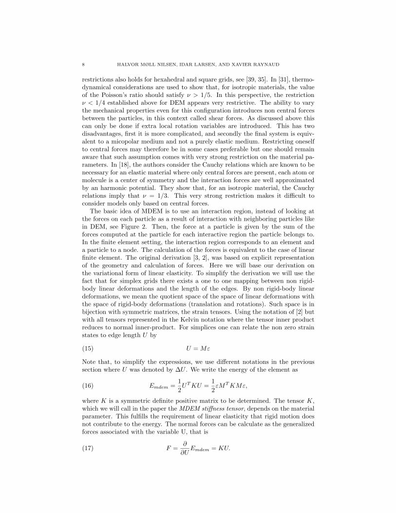
restrictions also holds for hexahedral and square grids, see [39, 35]. In [31], thermo-dynamical considerations are used to show that, for isotropic materials, the valueof the Poisson’s ratio should satisfy ν > 1/5. In this perspective, the restrictionν < 1/4 established above for DEM appears very restrictive. The ability to varythe mechanical properties even for this configuration introduces non central forcesbetween the particles, in this context called shear forces. As discussed above thiscan only be done if extra local rotation variables are introduced. This has twodisadvantages, first it is more complicated, and secondly the final system is equiv-alent to a micopolar medium and not a purely elastic medium. Restricting oneselfto central forces may therefore be in some cases preferable but one should remainaware that such assumption comes with very strong restriction on the material pa-rameters. In [18], the authors consider the Cauchy relations which are known to benecessary for an elastic material where only central forces are present, each atom ormolecule is a center of symmetry and the interaction forces are well approximatedby an harmonic potential. They show that, for an isotropic material, the Cauchyrelations imply that ν = 1/3. This very strong restriction makes it difficult toconsider models only based on central forces.
The basic idea of MDEM is to use an interaction region, instead of looking atthe forces on each particle as a result of interaction with neighboring particles likein DEM, see Figure 2. Then, the force at a particle is given by the sum of theforces computed at the particle for each interactive region the particle belongs to.In the finite element setting, the interaction region corresponds to an element anda particle to a node. The calculation of the forces is equivalent to the case of linearfinite element. The original derivation [3, 2], was based on explicit representationof the geometry and calculation of forces. Here we will base our derivation onthe variational form of linear elasticity. To simplify the derivation we will use thefact that for simplex grids there exists a one to one mapping between non rigid-body linear deformations and the length of the edges. By non rigid-body lineardeformations, we mean the quotient space of the space of linear deformations withthe space of rigid-body deformations (translation and rotations). Such space is inbijection with symmetric matrices, the strain tensors. Using the notation of [2] butwith all tensors represented in the Kelvin notation where the tensor inner productreduces to normal inner-product. For simplices one can relate the non zero strainstates to edge length U by
(15) U = Mε
Note that, to simplify the expressions, we use different notations in the previoussection where U was denoted by ∆U . We write the energy of the element as
(16) Emdem =1
2UTKU =
1
2εMTKMε,
where K is a symmetric definite positive matrix to be determined. The tensor K,which we will call in the paper the MDEM stiffness tensor, depends on the materialparameter. This fulfills the requirement of linear elasticity that rigid motion doesnot contribute to the energy. The normal forces can be calculate as the generalizedforces associated with the variable U, that is
(17) F =∂
∂UEmdem = KU.

COMBINING MDEM AND VEM FOR FRACTURING MODELING 9
From (17), we can see that assuming that only central forces are present and theshear forces are negligible is equivalent to the requirement that K is diagonal. Usingthe analogue definition of stress where we exploit the kelvin notation
(18) σ =∂
∂ε
(1
VEmdem
)=
1
VMTKMε =
1
VMTU.
If we consider the energy of the same system for a linear elastic media assumingconstant stress and strain, which is the case for linear elements on simplex grids,the result is
(19) Efem = V σ : ε = V εTDε
whereD is the representation of the forth order stiffness tensor C in Kelvin notation.Note also that epsi in (19) is meant either as a tensor (in the first equality) or asa vector written in Kelvin notations (in the second). For the sake of simplicity, wewill continue to do the same abuse of notations in the following. We see that onereproduces the energy of a linear elastic media if
(20) D = MTKM,
which gives that
(21) K = (M−1)TDM−1.
The difference between the matrix K used in DEM and the matrix needed toreproduce linear elasticity used in MDEM is that the latter case normally is a fullmatrix. Since DEM methods solve Newtons’s equation with a dissipation term itwill minimize this energy. The same is the case of standard Galerkin discretizationof linear FEM on simplices, which by construction have the same energy functionalas MDEM. Consequently, the only difference, if no fracture mechanism is presentwill be the method for computing the solution to the whole system of equations.The DEM methods rewrite the equations in the form of Newton laws with anartificial damping term and let time evolve to converge to the solution, see [10].For FEM, the linear equations are usually solved directly.
The advantage of using the MDEM formulation compared to FEM is that itoffers the flexibility to choose independently on each element if a force should becomputed using linear elasticity or if a more traditional DEM calculation shouldbe used.
The ability to associate the edge lengths to the non rigid body motions is onlypossible for simplex grids. An other important aspect to this derivation is that thedegrees of freedom uniquely define all linear motions and no others. The importanceof the last part will be more evident after comparison with the VEM method.
2.3. The Virtual Element Method. In contrast to FEM, the Virtual elementmethod seeks to provide consistency up to the right polynomial order of the equa-tion in the physical space. This is done by approximating the bilinear form onlyusing the definition of the degrees of freedom, as described below. The FEM frame-work on the other hand defines the assembly on reference elements, using a set ofspecific basis functions. This however has disadvantages for general grids wherethe mappings may be ill defined or complicated. VEM avoids this problem by onlyworking in physical space using virtual elements and not computing the Galerkinapproximation of the bilinear form exactly. This comes with a freedom in the

10 HALVOR MØLL NILSEN, IDAR LARSEN, AND XAVIER RAYNAUD
definition of the method and a cost in accuracy measured in term of the energynorm.
As the classical finite element method, the VE method starts from the linearelasticity equations written in the weak form of Equation 1,
(22)
∫Ω
ε(v) : Cε(u) dx =
∫Ω
v · f dx for all v.
We have also introduced the symmetric gradient ε given by
ε(u) = (∇+∇T )u,
for any displacement u. The fundamental idea in the VE method is to compute oneach element an approximation ahK of the bilinear form
(23) aK(u,v) =
∫K
ε(u) : Cε(v) dx,
that, in addition of being symmetric, positive definite and coercive with respect tothe non rigid-body motions, it is also exact for linear functions. The correspondencebetween MDEM and VEM we study here holds only for a first-order VEM method.When higher order methods are used, the exactness must hold for polynomials of agiven degree where the degree determines the order of the method. These methodswere first introduced as mimetic finite element methods but later developed furtherunder the name of virtual element methods (see [11] for discussions). The degreesof freedom are chosen as in the standard finite element methods to ensure thecontinuity at the boundaries and an element-wise assembly of the bilinear forms ahK .We have followed the implementation described in [14]. In a first-order VE method,the projection operator P into the space of linear displacement with respect to theenergy norm has to be computed locally for each cell. The VE approach ensuresthat the projection operator can be computed exactly for each basis element. Theprojection operator is defined with respect to the metric induced by the bilinearform aK . The projection is self-adjoint so that we have the following Pythagorasidentity,
(24) aK(u,v) = aK(Pu,Pv) + aK((I−P)u, (I−P)v)
for all displacement field u and v (in order to keep this introduction simple, wedo not state the requirements on regularity which is needed for the displacementfields). In [14], an explicit expression for P is given so that we do not even have tocompute the projection. Indeed, we have P = PR +PC where PR is the projectionon the space R of translations and pure rotations and PC the projection on thespace C of linear strain displacement. The spaces R and C are defined as
R =a +B(x− x) | a ∈ R3, B ∈ R3×3, BT = −B
,
C =B(x− x) | B ∈ R3×3, BT = B
.
Then, the discrete bilinear form ahK is defined as
(25) ahK(u,v) = aK(Pu,Pv) + sK((I−P)u, (I−P)v)
where sK is a symmetric positive matrix which is chosen such that ahK remainscoercive. Note the similarities between (25) and (24). Since PR and PC are orthog-onal and PR maps into the null space of aK (rotations do not produce any change

COMBINING MDEM AND VEM FOR FRACTURING MODELING 11
|E| |F |
Exact assembly of energyfor linear functions
Projection tolinear displacement
Wc
R
M−1
Addregularization term(I − P )tS(I − P )
back to virtual basisWT
c
(M−1)T
RT
Figure 2. This show the difference and similarities of the MDEMand the VEM framework.
in the energy), we have that the first term on the right-hand side of (24) and (25)can be simplified to
aK(Pu,Pv) = aK(PCu,PCv).
The expression (25) immediately guarantees the consistency of the method, as weget from (25) that, for linear displacements, the discrete energy coincides withthe exact energy. Since the projection operator can be computed exactly for allelements in the basis - and in particular for the virtual basis elements for which wedo not have explicit expressions - the local matrix can be written only in terms ofthe degrees of freedom of the method. In our case the degrees of freedom of themethod are the value of displacement at the node. Let us denote ϕi a basis forthese degrees of freedom. The matrix (AK)i,j = ahK(ϕi,ϕj) is given by
(26) AK = |K| WTCDWC + (I−P)TSK(I−P).
In (26), WC is the projection operator from the values of node displacements tothe space of constant shear strain and SK , which corresponds to a discretization ofSK in (25), is a symmetric positive matrix which guarantees the positivity of AK .There is a large amount of freedom in the choice of SK but it has to scale correctly.We choose the same SK as in [14]. The matrix D in (26) corresponds to the tensorC rewritten in Kelvin notations so that, in three dimensions, we have
Dij = εi : Cεj , for i, j = 1, . . . , 6.
Finally, the matrices AK are used to assemble the global matrix A correspondingto ah. In this paper, we use the implementation available as open source throughthe Matlab Reservoir Simulation Toolbox (MRST) [32]. The approach of splittingthe calculation of the energy in terms of a consistent part block on one side anda higher order block one the other side was also used in the free formulation offinite elements [6]. In this case the motivation was to find an alternative elementformulation,
2.4. Correspondences between VEM and MDEM. For simplex grids the reg-ularization term SK in the expression for the local stiffness matrix in Equation 26is zero because in this case the projection operator is equal to the identity. If we

12 HALVOR MØLL NILSEN, IDAR LARSEN, AND XAVIER RAYNAUD
introduce the operator from the degrees of freedom for the element to the edgeexpansions R, we can compare the two expression for the local energy,
(27a) Evem = uT |K|WTCDWCu
and
(27b) Emdem = uTRTKRu = uT |K|RT (M−1)TDM−1RTu.
One easily identifies the operators WC and M−1RT as the projection operatorPc tothe non-rigid body motions represented in Kelvin notation type of symmetric strain.The degrees of freedom span exactly the space of linear displacement and do notexcite any higher order modes with nonzero energy. An illustration of the differentconcepts is given in Figure 2. We point that both DEM and VEM calculate thebasic stiffness matrix in real space, contrary to most FEM methods which do thison the reference element. When dealing with simplex grids the advantage of usingthe DEM method within an explicit solving strategy (often called distinct elementmethod) is that the calculation of the edge length extensions U can be calculated foreach edge, and only the matrices M−1 and the Cauchy stiffness tensor C are neededlocally. These matrices only operate on the small space of non rigid motion withdimension ((d(d+ 1))/2) while the operator Wc works on the all the deformationswhich have dimension ((d+ 1)d). The edge length can thus be seen as an efficientcompact representation of the non rigid motions, which holds only on simplices. Aswe have seen, both MDEM and VEM can be derived from the calculation of theenergy in each element. For the linear elastic part it is not necessary to introduceextra angular degrees of freedom. However, this may be needed for certain DEMmethods. In this case, we refer to the use of drilling elements in combinationwith the use of the free formulation of FEM [13, 7], which, as discussed earlier,shares some fundamental ideas with VEM, such as energy orthogonality (whichcorresponds (24)), and rc-modes exactness (whic) and the freedom in choosing thestabilization term.
2.5. Fluid mechanics coupling. We introduce a coupling with a fluid flow throughthe Biot’s equations [8]. The Biot’s equations are given by
∇ · σ +∇p = f ,(28a)
∂
∂t(Scp+ α∇ · u) +∇ · (K
µv∇p) = 0,(28b)
where Scp + α∇ · u denotes the fluid content. The fluid content depends on thestorativity Sc, the fluid pressure p and on the rock volume change given by ∇ · uwhich is weighted by the Biot-Willis constant α. In (28), K denotes the permeabilityand µv the fluid viscosity. For flow, and in particular if multiphase behaviors areconsidered, the most successful methods have been based on finite volume methods.The basic time discretization using the two point flux method or multi point fluxmethods [1] can be written as
(29) Scpn+1 − pn
∆t− divf
[K
µvgradp
[pn+1
]]= Q.
Here gradp is a discrete gradient operator from cell pressures to face, divf is the cor-responding discrete divergence acting on face fluxes. The source term Q representsthe injection of fluids, see [24] for more details on those discrete operators.
COMBINING MDEM AND VEM FOR FRACTURING MODELING 13
Given an implicit time discretization the coupling term in the Biot case requiresa discrete divergence operator divd for displacement field. Note that this discreteoperator can be implemented exactly for first order VEM, see [37] for more details.The semi-discrete equations are(30)
As un+1 − αdivTd[pn+1
]= −F
αdivd[un+1
]+ Scp
n+1 −∆tdivf
[Kµv
gradp[pn+1
]]= αdivd [un] + Scp
n +Q.
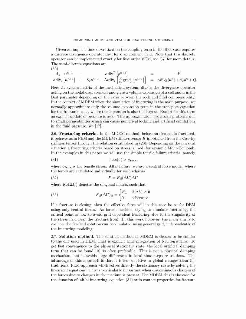
Here As system matrix of the mechanical system, divd is the divergence operatoracting on the nodal displacement and gives a volume expansion of a cell and α is theBiot parameter depending on the ratio between the rock and fluid compressibility.In the context of MDEM when the simulation of fracturing is the main purpose, wenormally approximate only the volume expansion term in the transport equationfor the fractured cells, where the expansion is also the largest. Except for this terman explicit update of pressure is used. This approximation also avoids problems dueto small permeabilities which can cause numerical locking and artificial oscillationsin the fluid pressure, see [17].
2.6. Fracturing criteria. In the MDEM method, before an element is fractured,it behaves as in FEM and the MDEM stiffness tensor K is obtained from the Cauchystiffness tensor through the relation established in (20). Depending on the physicalsituation a fracturing criteria based on stress is used, for example Mohr-Coulomb.In the examples in this paper we will use the simple tensile failure criteria, namely
(31) max(σ) > σtens,
where σtens is the tensile stress. After failure, we use a central force model, wherethe forces are calculated individually for each edge as
(32) F = Kd(∆U)∆U
where Kd(∆U) denotes the diagonal matrix such that
(33) Kd(∆U)ii =
Kii if ∆Ui < 0
0 otherwise
If a fracture is closing, then the effective force will in this case be as for DEMusing only central forces. As for all methods trying to simulate fracturing, thecritical point is how to avoid grid dependent fracturing, due to the singularity ofthe stress field near the fracture front. In this work however, the main aim is tosee how the far-field solution can be simulated using general grid, independently ofthe fracturing modeling.
2.7. Solution method. The solution method in MDEM is chosen to be similarto the one used in DEM. That is explicit time integration of Newton’s laws. Toget fast convergence to the physical stationary state, the local artificial dampingterm that can be found [10] is often preferable. This is not a physical dampingmechanism, but it avoids large differences in local time steps restrictions. Theadvantage of this approach is that it is less sensitive to global changes than thetraditional FEM approach which solves directly the stationary state by solving thelinearized equations. This is particularly important when discontinuous changes ofthe forces due to changes in the medium is present. For MDEM this is the case forthe situation of initial fracturing, equation (31) or in contact properties for fracture

14 HALVOR MØLL NILSEN, IDAR LARSEN, AND XAVIER RAYNAUD
T11 T22 T33
T23 T13 T12
Figure 3. The figure shows the difference of the mechanical pa-rameters between the DEM fracture model (32) and linear elas-ticity, in the case of compression in all edges. Here, T = C −K−1(K(C)d) and the six components of T are plotted.
cells, equation (32). The result in all cases is that the forces are discontinuouswith respect to the degrees of freedom. Explicit methods have been shown to haveadvantages for such problems even if the main dynamics is globally elliptic, becausethe non-linearities in the problem impose stronger time-step size requirement thatthose needed for the explicit integration of the elliptic part. As the damping criteriadepends on the concept of total nodal forces, it can also be used on the nodesconnected with VEM type of force calculations. No other modification apart fromthe force calculations are needed.
3. Examples
We demonstrate the features of the presented framework with two examples.First we show how the effective parameters of linear elasticity in simple DEM withonly normal forces depend on the particular choice of the grid cells. Second, we useVEM, MDEM and DEM on a general a polyhedral grid to demonstrate how thiscan be combined within a uniform framework.
When a fracture has occurred in a cell, but the whole system evolves in sucha way that the fracture closes again, then we should have forces normal to thefracture faces and, depending on the fracture model, forces along the fracture.Here, we choose to model this by an effective stiffness tensor. Indeed, we keepusing the DEM model (and solver) after the fracture closes, meaning that themateriel parameters for the cell are given by the diagonal MDEM stiffness tensorKd as defined in (33). From Section 2.4, we know that it also corresponds to aunique Cauchy stiffness tensor. Let us study the effect of such choice and measurethe difference between the original and this post-fracturing stiffness tensor. If wedenote by K, the one-to-one transformation from the MDEM stiffness tensor K tothe Cauchy stiffness tensor C, we compute, for a given C, the difference betweenC and K−1(K(C)d). We consider a equilateral triangle and an isotropic material

COMBINING MDEM AND VEM FOR FRACTURING MODELING 15
Figure 4. The figure shows a fracture growing in the directionperpendicular to the maximum stress. Pressure in and divergenceof the solution is given in upper left and right respectively. In themiddle the displacement in the x direction, left, and y is plotted.At the bottom the figure show the minimal stress left and themaximum stress right. The cells in red correspond do fracturedcells. The blue and the red and blue lines is show the direction ofthe principle axis for maximum and minimum stress respectively.Both pressure and stress is given in 105Pa.
with Young’s modulus E = 1 and Poison ratio ν = 1/4. For this value of ν andthis shape, the matrix K is diagonal, so that C = K−1(K(C)d). This referencetriangle is plotted in yellow in Figure 3. We keep the same Cauchy stiffness tensorbut modify the shape of the triangle by translating one of the corners. For eachconfiguration that is obtained, we get a different post-fracturing MDEM stiffnesstensor given by K(C)d and we plot the six component of the tensor T defined as

16 HALVOR MØLL NILSEN, IDAR LARSEN, AND XAVIER RAYNAUD
Figure 5. The figure show an large picture of the maximum stressshown in lower right corner of figure 4. The left figure are using thestress form the linear elements while the right are from the stressusing patch recovery.
the difference T = C − K−1(K(C)d). We notice that the changes in C2,3 and C1,3
is zero when on the line x = 0 in the figure. This show that in this case as expectedthe effective model has biaxial symmetry. We also notice that there is quite strongchanges in the effective parameters even for relatively small changes in the triangles.It should also be noted that a break of the edges along the x-axis, which in theMDEM fracture model result in putting one of the corresponding diagonal elementto zero only changes the value of C1,1. This is because this only acts in the xdirection.
We use MRST [32, 27] to generate the unstructured grid presented in Figure 4and set up an example which combines the use of VEM for the general cell shapesand the use of MDEM for the triangular cells that can easily be switched to a DEMmodel when a fracture is created. The total grid size is 30 m× 30 m. In the middlewithin a diameter 0.5 m we have placed cells associated with a well. The perme-ability used was 10 nd, porosity of 0.3, the compressibility of the fluid is similar towater, 1× 10⁻¹⁰ Pa−1, and it is injected fluid corresponding to the pore volume ofall well cells in an hour. The solution is shown after 40 minutes. The initial con-dition was given by the mechanical solution with a force of 1× 10⁷ Pa at the topand rolling all other places. The initial condition for pressure is constant pressureequal to 1× 10⁷ Pa. The mechanical parameters are given by E = 1× 10⁹ Pa andν = 0.3. The well cells are set to have Young’s modulo E = 1× 10⁴ Pa and finallythe tensile strength is 2× 10⁵ Pa. We observe that the fracture propagates in thedirection so that the fracture plane (or line in 2D) is aligned with the maximumstress plane (or line in 2D). We get slight grid orientation effect since there is noway a planar fault in the y direction can be obtain using the given triangular grid.The interface between the grids has large steps in cell sizes and include hangingnodes, but no effects due to these features are observed as long as the fracture doesnot reach the interface. Near the tip of the fracture we observe oscillation of thestress on cells, which is a well known problem for first order triangular elements.However the values associate with the nodes is better approximated and patch re-covery techniques [41] can be used to get better stress fields as seen in Figure 5.A note is that the dynamics of DEM or MDEM, is associated with the sum of allforces from all elements around a node, not individual stresses for cells.

COMBINING MDEM AND VEM FOR FRACTURING MODELING 17
4. Conclusions
In this paper we have shown how MDEM and VEM for linear elasticity sharethe same basic idea of projection to the states of linear non-rigid motions, althoughwith different representations, length extension for MDEM and polynomial basisfor VEM. Both are equivalent to linear FEM on simplices, but the viewpoint pre-sented here gives a more direct way on how they relate. Since both share the samedegrees of freedom, except possibly the angular degree of freedom of MDEM/DEM,we combine these methods with minimal implementation issues. This is used tosimulate fracture growth, where the near field regions is described by a simplexgrid which is suited for DEM and MDEM, while the general polyhedral grids isused in the far-field region. The coupling between the grids which can containhanging nodes and significant changes in cell shapes and sizes, can be done withoutintroducing large errors. We see this method as a valuable contribution to flexiblecoupling of MDEM/DEM methods with traditional reservoir modeling grids.
5. Acknowledgments
This publication has been produced with support from the KPN project Con-trolled Fracturing for Increased Recovery. The authors acknowledge the follow-ing partners for their contributions: Lundin and the Research Council of Norway(244506/E30).
References
[1] Ivar Aavatsmark. An introduction to multipoint flux approximations for quadrilateral grids.
Computational Geosciences, 6(3-4):405–432, 2002.[2] Haitham Alassi, Rune Holt, and Martin Landrø. Relating 4d seismics to reservoir geome-
chanical changes using a discrete element approach. Geophysical Prospecting, 58(4):657–668,
2010.[3] Haitham Tayseer Alassi. Modeling reservoir geomechanicsusing discrete element method :
Application to reservoir monitoring. PhD thesis, NTNU, 2008.
[4] Haitham Tayseer Alassi and Rune Holt. Relating discrete element method parameters torock properties using classical and micropolar elasticity theories. International Journal for
Numerical and Analytical Methods in Geomechanics, 36(10):1350–1367, 2012.[5] D.J. Allman. Special memorial issue a compatible triangular element including vertex rota-
tions for plane elasticity analysis. Computers & Structures, 19(1):1 – 8, 1984.
[6] P. G. Bergan and M. K. Nygard. Free formulation elements applied to stability of shells.
Computational Mechanics, pages 914–919, 1988.[7] P. G. Bergan, M. K. Nygard, and R. O. Bjærum. Computational Mechanics of Nonlinear
Response of Shells, chapter Free Formulation Elements with Drilling Freedoms for StabilityAnalysis of Shells, pages 164–182. Springer Berlin Heidelberg, Berlin, Heidelberg, 1990.
[8] Maurice A Biot. General theory of three-dimensional consolidation. Journal of applied
physics, 12(2):155–164, 1941.[9] Robert D. Cook. On the allman triangle and a related quadrilateral element. Computers &
Structures, 22(6):1065 – 1067, 1986.
[10] P. A. Cundall and O. D. L. Strack. A discrete numerical model for granular assemblies.Geotechnique, 29(1):47–65, 1979.
[11] Lourenco Beirao da Veiga, Konstantin Lipnikov, and Gianmarco Manzini. Mimetic Finite
Difference Method for Elliptic Problems, volume 11. Springer, 2014.[12] Jack Dvorkin and Amos Nur. Elasticity of high-porosity sandstones: Theory for two north
sea data sets. Geophysics, 61(5):1363–1370, 1996.
[13] Carlos A. Felippa. A study of optimal membrane triangles with drilling freedoms. ComputerMethods in Applied Mechanics and Engineering, 192(16-18):2125 – 2168, 2003.

18 HALVOR MØLL NILSEN, IDAR LARSEN, AND XAVIER RAYNAUD
[14] Arun L Gain, Cameron Talischi, and Glaucio H Paulino. On the virtual element method
for three-dimensional linear elasticity problems on arbitrary polyhedral meshes. Computer
Methods in Applied Mechanics and Engineering, 282:132–160, 2014.[15] A. A. Griffith. The phenomena of rupture and flow in solids. Philosophical Transactions of
the Royal Society of London A: Mathematical, Physical and Engineering Sciences, 221(582-
593):163–198, 1921.[16] Emmanuel J. Gringarten, Guven Burc Arpat, Mohamed Aymen Haouesse, Anne Dutranois,
Laurent Deny, Stanislas Jayr, Anne-Laure Tertois, Jean-Laurent Mallet, Andrea Bernal, and
Long X. Nghiem. New grids for robust reservoir modeling. SPE Annual Technical Conferenceand Exhibition, 2008.
[17] Joachim Berdal Haga, Harald Osnes, and Hans Petter Langtangen. On the causes of pressure
oscillations in low-permeable and low-compressible porous media. International Journal forNumerical and Analytical Methods in Geomechanics, 36(12):1507–1522, 2012.
[18] Friedrich W. Hehl and Yakov Itin. The cauchy relations in linear elasticity theory. Journalof elasticity and the physical science of solids, 66(2):185–192, 2002.
[19] Klaus Helbig. Review paper: What kelvin might have written about elasticity. Geophysical
Prospecting, 61(1):1–20, 2013.[20] Thomas J.R. Hughes and F. Brezzi. On drilling degrees of freedom. Computer Methods in
Applied Mechanics and Engineering, 72(1):105 – 121, 1989.
[21] T.J.R. Hughes, A. Masud, and I. Harari. Numerical assessment of some membrane elementswith drilling degrees of freedom. Computers & Structures, 55(2):297–314, Apr 1995.
[22] International Energy Agency, 2015.
[23] L. Jing and J.A. Hudson. Numerical methods in rock mechanics. International Journal ofRock Mechanics and Mining Sciences, 39(4):409–427, 2002. cited By 190.
[24] Stein Krogstad, Knut-Andreas Lie, Olav Møyner, Halvor Møll Nilsen, Xavier Raynaud, Bard
Skaflestad, et al. Mrst-ad–an open-source framework for rapid prototyping and evaluation ofreservoir simulation problems. In SPE reservoir simulation symposium. Society of Petroleum
Engineers, 2015.[25] Meinhard Kuna. Finite elements in fracture mechanics. Solid Mechanics and Its Applications,
2013.
[26] Quanshu Li, Huilin Xing, Jianjun Liu, and Xiangchon Liu. A review on hydraulic fracturingof unconventional reservoir. Petroleum, 1(1):8 – 15, 2015.
[27] Knut-Andreas Lie, Stein Krogstad, Ingeborg Skjelkvale Ligaarden, Jostein Roald Natvig,
Halvor Nilsen, and Bard Skaflestad. Open-source MATLAB implementation of consistentdiscretisations on complex grids. Comput. Geosci., 16:297–322, 2012.
[28] A. Lisjak and G. Grasselli. A review of discrete modeling techniques for fracturing processes
in discontinuous rock masses. Journal of Rock Mechanics and Geotechnical Engineering,6(4):301–314, 2014.
[29] Bradley Mallison, Charles Sword, Thomas Viard, William Milliken, and Amy Cheng. Un-
structured cut-cell grids for modeling complex reservoirs. SPE Journal, 19(02):340–352, Apr2014.
[30] R. D. Mindlin. Compliance of elastic bodies in contact. J. Applied Mechanics, 16:259– 268,1949.
[31] P H Mott and C M Roland. Limits to poisson’s ratio in isotropic materials-general result for
arbitrary deformation. Physica Scripta, 87(5):055404, 2013.[32] The MATLAB Reservoir Simulation Toolbox, version 2016a, 7 2016.
[33] Rajendra K. Pachauri and Leo Meyer. Climate change 2007: synthesis report. summary forpolicymakers. IPCC, 2014.
[34] X.D. Pan and M.B. Reed. A coupled distinct element-finite element method for large deforma-
tion analysis of rock masses. International Journal of Rock Mechanics and Mining Sciences
& Geomechanics Abstracts, 28(1):93–99, Jan 1991.[35] I.S. Pavlov, A.I. Potapov, and G.A. Maugin. A 2d granular medium with rotating particles.
International Journal of Solids and Structures, 43(20):6194 – 6207, 2006.[36] David K Ponting. Corner point geometry in reservoir simulation. In ECMOR I-1st European
Conference on the Mathematics of Oil Recovery, 1989.
[37] Xavier Raynaud, Halvor Møll Nilsen, and Odd Andersen. Virtual element method for geome-
chanical simulations of reservoir models. In ECMOR XV–15th European Conference on theMathematics of Oil Recovery, Amsterdam, Netherlands, 2016.

COMBINING MDEM AND VEM FOR FRACTURING MODELING 19
[38] W. Schubert and Ed. Essen, editors. Novel Approach to Studying Rock Damage: The Three
Dimensional Adaptive Continuum / Discontinuum Code. Proceedings, ISRM Regional Sym-
posium EUROCK 2004 and 53rd Geomechanics Colloquy, Salzburg, Verlag Gluckauf, 2004.[39] A.S.J. Suiker, A.V. Metrikine, and R. de Borst. Comparison of wave propagation characteris-
tics of the cosserat continuum model and corresponding discrete lattice models. International
Journal of Solids and Structures, 38(9):1563 – 1583, 2001.[40] K. Walton. The effective elastic moduli of a random packing of spheres. Journal of the Me-
chanics and Physics of Solids, 35(2):213 – 226, 1987.
[41] O. C. Zienkiewicz and J. Z. Zhu. The superconvergent patch recovery and a posteriori errorestimates. part 1: The recovery technique. International Journal for Numerical Methods in
Engineering, 33(7):1331–1364, 1992.