combining related products into product lineschechik/pubs/fase12.pdf · combining related products...

Combining Related Products into Product Lines

Julia Rubin1,2 and Marsha Chechik1

1 University of Toronto, Canada2 IBM Research in Haifa, Israel

[email protected] [email protected]

Abstract. We address the problem of refactoring existing, closely related prod-ucts into product line representations. Our approach is based on comparing andmatching artifacts of these existing products and merging those deemed simi-lar while explicating those that vary. Our work focuses on formal specificationof a product line refactoring operator called merge-in that puts individual prod-ucts together into product lines. We state sufficient conditions of model compare,match and merge operators that allow application of merge-in. Based on these,we formally prove correctness of the merge-in operator. We also demonstrate itsoperation on a small but realistic example.

1 IntroductionNumerous companies develop and maintain families of related software products. Theseproducts share a common, managed set of features that satisfy the specific needs of aparticular market segment and are referred to as software product lines (SPLs) [4]. SPLsoften emerge from experiences in successfully addressed markets with similar, yet notidentical needs. It is difficult to foresee these needs a priori and hence to structure andmanage the SPL development upfront [11]. As a result, SPLs are usually developed inan ad-hoc manner, using available software engineering practices such as duplication(the “clone-and-own” paradigm where artifacts are copied and modified to fit the newpurpose), inheritance, source control branching and more. However, these software en-gineering practices do not scale well to product line development, resulting in massiverework, increased time-to-market and lost opportunities.

Software Product Line Engineering (SPLE) is a software engineering disciplineaiming to provide methods for dealing with the complexity of SPL development [4,18, 5]. SPLE practices promote systematic software reuse by identifying and managingcommonalities – artifacts that are part of each product of the product line, and variabil-ities – artifacts that are specific to one or more (but not all) individual products acrossthe whole product portfolio. Commonalities and variabilities are controlled by featuremodels [7] (a.k.a. variability models) which specify program functionality units and re-lationships between them. A product of the product line is identified by a unique andlegal combination of features, and vice versa.

SPLE approaches can be divided into two categories: compositional, which imple-ment product features as distinct fragments and allow generating specific product bycomposing a set of fragments, and annotative, which assume that there is one “max-imal” product in which annotations indicate the product feature that a particular frag-ment realizes [8, 3]. A specific product is obtained by removing fragments correspond-ing to discarded features. We follow the annotative approach here.

A number of works, e.g., [18, 5], promote the use of annotative SPLE practicesfor model-driven development of complex systems. They are built upon the idea ofexplicating and parameterizing variable model elements by features. The parameterizedelements are included in a product only if their corresponding features are selected,allowing coherent and uniform treatment of the product portfolio, a reduced number ofduplications across products, better understandability and reduced maintenance effort,e.g., because modifications in the common parts can be performed only once.

Weighing

Unlocking WashingDrying

Locking[<=5kg][>5kg] /displayError();

/dryer.sendSignal(SigStart);SigDone()

/wash.sendSignal(SigStart);

SigDone()

(a) Controller A.

Weighing

Unlocking Washing

Locking

Waiting

[<=5kg][>5kg] /displayError();

/wash.wtrLevel=weight*0.5;wash.sendSignal(SigStart);SigDone()

/timer.sendSignal(SigStart);

SigDone()

(b) Controller B.

Weighing

Beeping Unlocking Washing

Locking[<=6kg][>6kg] /displayError();

/wash.wtrLevel=weight*0.5;wash.sendSignal(SigStart);

/beeper.sendSignal(SigStart); SigDone()

SigDone()

(c) Controller C.Fig. 1. Washing Machine Controllers.

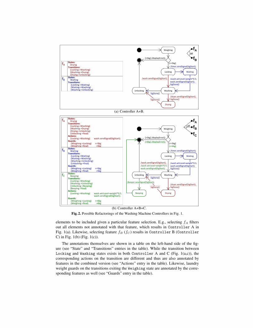
Example. Consider three fragments ofUML statechart controllers depicted inFig. 1. These models were inspired by areal-life SPL developed by a partner (sincepartner-specific details are confidential, wemove the problem into a familiar domainof washing machines). Controller A inFig. 1(a) weighs the laundry and displays anerror message if the weight is more than 5kg. Otherwise, it locks the washing machineand sends a signal to the wash engine, re-sponsible for performing the washing cycle.When washing is done, the Controller

signals the dryer to perform the drying cy-cle, after which it proceeds to unlock thewashing machine and finish. ControllerB in Fig. 1(b) differs from the one inFig. 1(a) by using the timer componentto delay the wash cycle and by setting thewtrLevel attribute of the wash engine tothe desired water level based on the weightof the laundry. This model also lacks thedryer capability. Similarly to the one inFig. 1(b), Controller C in Fig. 1(c) usesthe wtrLevel attribute to set the desiredwater level of the wash engine based on thelaundry weight. However, it allows laundryweights up to 6 kg. It also lacks both thedryer and the timer capabilities but initiatesan acoustic notification at the end of theprogram by invoking the beeper engine.

These controllers have a large degree of similarity and can be refactored into SPLErepresentations where duplications are eliminated and variabilities are explicated. Anexample of a possible refactoring is given in Fig. 2(b), where the Drying, Waiting andBeeping states and their corresponding transitions are annotated by a set of featuresdepicted in the right upper part of the figure. The refactored product line in our exam-ple encapsulates only the original input products, thus we have just three alternativefeatures representing these products – fA, fB and fC . The set of annotations specifies

Weighing

Unlocking Washing

Drying

Locking Waiting

[<=5kg]

[>5kg] /displayError();



SigDone()



SigDone()

fAalt

fB

fA States: Drying Transitions: (Locking->Washing) (Washing->Drying) (Drying->Unlocking)

fB

States: Waiting Transitions: (Locking->Waiting) (Waiting->Washing) (Washing->Unlocking)

(a) Controller A+B.

fAalt fB

fC

Weighing

Beeping

Unlocking Washing

Drying

Locking Waiting

[<=5kg][<=6kg]



/wash.wtrLevel=weight*0.5;wash.sendSignal(SigStart);

/beeper.sendSignal(SigStart);



SigDone()



SigDone()

fA

States: Drying Transitions: (Locking->Washing) (Washing->Drying) (Drying->Unlocking) (Unlocking->final) Actions: (Locking->Washing) wash.sendSignal(SigStart); Guards: (Weighing->Locking) <=5kg (Weighing->final) >5kg

fB

States: Waiting Transitions: (Locking->Waiting) (Waiting->Washing) (Washing->Unlocking) (Unlocking->final) Guards: (Weighing->Locking) <=5kg (Weighing->final) >5kg

fC

States: Beeping Transitions: (Locking->Washing) (Washing->Unlocking) (Unlocking->Beeping) (Beeping->final) Actions: (Locking->Washing) wash.wtrLevel=weight*0,5; wash.sendSignal(SigStart); Guards: (Weighing->Locking) <=6kg (Weighing->final) >6kg

(b) Controller A+B+C.Fig. 2. Possible Refactorings of the Washing Machine Controllers in Fig. 1.

elements to be included given a particular feature selection. E.g., selecting fA filtersout all elements not annotated with that feature, which results in Controller A inFig. 1(a). Likewise, selecting feature fB (fC) results in Controller B (ControllerC) in Fig. 1(b) (Fig. 1(c)).

The annotations themselves are shown in a table on the left-hand side of the fig-ure (see “State” and “Transitions” entries in the table). While the transition betweenLocking and Washing states exists in both Controller A and C (Fig. 1(a,c)), thecorresponding actions on the transition are different and thus are also annotated byfeatures in the combined version (see “Actions” entry in the table). Likewise, laundryweight guards on the transitions exiting the Weighing state are annotated by the corre-sponding features as well (see “Guards” entry in the table).

Product Line Refactoring Framework. Despite the benefits of applying SPLE prac-tices which include improved time-to-market and quality, reduced portfolio size, engi-neering costs and more [4], it is impractical to assume that existing (legacy) productline systems can be abandoned altogether for creating new ones that take advantageof the SPLE reuse techniques. Thus, a transition process which involves identificationand extraction of common and variable artifacts together with variability models thatcontrol them, becomes a necessity [12, 1].

In our work, we propose a generic framework for mining legacy product lines andautomating their refactoring to contemporary feature-oriented SPLE approaches, ini-tially suggested in [19]. We consider those refactorings that just include the set of exist-ing products rather than allowing novel feature combinations (e.g., a product with boththe timer and the beeper capabilities). Our approach is based on comparing elementsof the input products to each other (by calculating a weighted similarity of their cor-responding sub-elements), matching those whose similarity is above a preset thresholdand merging these together.

Our refactoring framework is applicable to a variety of model types, such as UML,EMF or Matlab/Simulink, and to different compare, match and merge operators. In thispaper, we develop a generic model representation and a generic and parameterizablecompare / match / merge infrastructure underlying the refactoring framework. Usingthem, we prove that our refactoring approach is semantically correct, i.e., it can gen-erate exactly the original products, regardless of a particular implementation used andparameters chosen. The main contribution of this paper is thus the formal foundationthat underlays the parameterizable and configurable, yet semantically correct refactor-ing framework.

There are multiple ways to merge-in input products into a product line, even if weonly consider those refactorings that maintain the original set of input products. Theresulting refactorings vary syntactically, depending on how elements are matched andcombined. For example, in Fig. 2(b), transitions from Locking to Washing states ofControllers A and C (Fig. 1 (a,c)) are matched to each other and combined, whiletheir corresponding actions are annotated by features. Instead, these transitions do nothave to be matched, so that the generated result has two separate transitions, each an-notated by the corresponding feature. Also, the Unlocking state of Controller A inFig. 1(a) could be matched and combined with the Beeping state of Controller C inFig. 1(c) because of their structural similarity – both transition to the final state of thestatechart.

In this work, we formally prove that all these syntactically different refactorings areable to produce the set of original input products and thus are “correct”. Elsewhere [20],we focus on techniques for distinguishing between multiple possible refactorings basedon their qualitative properties and choosing a desired one which satisfies the set of de-fined objectives (e.g., one objective might be to decrease the size of the produced result,while another – to keep a low number of annotated elements per diagram). In [20], wealso instantiate our approach on product lines defined in UML – a common specifica-tion language in automotive, aerospace & defense, and consumer electronics domains,and demonstrate its applicability on several large-scale examples.

The remainder of this paper is organized as follows. We introduce our data modeland give the necessary background on product lines representations in Sec. 2. We giveformal foundations of model merging in Sec. 3 and define our merging-based productline refactoring technique in Sec. 4. We prove semantic correctness of the technique inSec. 5. We conclude the paper with a discussion of related work in Sec. 6, presenting asummary and future research directions in Sec. 7.

2 PreliminariesIn this section, we describe our representation of models and model elements and fixour notation for representing product line models annotated by features.

Model Representation. Following XMI principles [17], we define models to be trees oftyped elements. Each element has a unique id which identifies it within the model anda role which defines the relationship between the element and its parent. For example,in UML, an element of type Behavior can have an Entry action or Do activity rolesin a state. In addition, a single element can fulfill several roles in a model: a Behaviorcan be a Do activity of a state and an Effect of a transition at the same time. To allowreusing elements for different roles, we employ a cross-referencing mechanism wherean element of type Ref represents the referenced element by carrying its id. Cross-referencing, combined with roles, allows representing labeled graphs using trees: anelement can be linked to multiple different elements, each time in a distinct role.

Element types, denoted by T, and roles, denoted by R, are defined by the domainmodel. For UML, types include Class, State, OpaqueBehavior, etc. Roles includePackagedElement, Subvertex, Effect, etc. If the types Ref and String are notdefined by the domain model, we add them to T as well.

We differ from [17] by representing all element attributes, as first-class model ele-ments. That is, an element’s name is represented by a separate model element of roleName and type String. The implication of our representation is that elements’ attributesnow have their own ids and thus, an element can have multiple attributes in the samerole, e.g., multiple names or Effects for a transition. These qualities are required fordefining the product line merge-in operator in Sec. 4. A formal representation of ournotations is given by Def. 1 below.Definition 1. (Model Element) A model element m is a tuple 〈m|id,m|t,m|r,m|v, m|s〉,where m|id is a numeric identifier of the element, m|t ∈ T is the element’s type, m|r ∈ Ris the element’s role, m|v is the element’s value – either String or an id of another element(representing a reference), and m|s is a (nested) list of sub-elements.

Fig. 3 shows partial representation of the Controller A statechart in Fig. 1(a),where states Drying and Unlocking, together with their incoming and outgoing transi-tions, are omitted to save space. In this figure, sub-elements are represented as element’schildren in the tree.

We refer to types that have no owned properties, such as String or Ref, as atomic.Other types, such as Class, State or Transition, are compound. Elements of atomicand compound types are referred to as atomic and compound elements, respectively.While atomic elements have values, values of compound elements are determined fromvalues of their sub-elements. Thus, two compound elements may be equal (i.e., havethe same type and role, like elements with ids 3 and 6 in Fig. 3) but not equivalent, asthey might have different sub-elements.

id = 1t = StateMachiner = OwnedBehaviour

id = 2t = Pseudostater = Subvertexv = start

id = 3t = Stater = Subvertex

id = 4t = Stringr = Namev = Weighing

id = 15t = Transitionr = Transition

id = 16t = Referencer = Sourcev = 2

id = 17t = Referencer = Targetv = 3


id = 7t = Stringr = Namev = Locking


id = 9t = Stringr = Namev = Washing

id = 5t = Pseudostater = Subvertexv = choice

id = 14t = FinalStater = Subvertex




id = 24t = Constraintr = OwnedRulev = <=5kg




id = 28t = Constraintr = OwnedRulev = >5kg

id = 29t = OpaqueBehav.r = Effectv = displayError();



id = 20t = Referencer = Targetv = 5...

...




id = 33t = OpaqueBehav.r = Effectv = wash.

sendSignal (SigStart);

Fig. 3. Partial representation of the Statechart in Fig. 1(a).

Definition 2. (Equivalence) Given a universe of model elements M, let M1,M2 ∈ 2M bedistinct sets of elements.m1 ∈M1,m2 ∈M2 are equal, denoted bym1

∼= m2, iffm1|t = m2|t,m1|r = m2|r andm1|v = m2|v . Equal atomic elements are equivalent. Compound elements areequivalent, denoted by m1 = m2, iff m1

∼= m2, and their corresponding trees of sub-elementsare isomorphic wrt. equality.

Definition 3. (Model and Model Equivalence) A set of elements M ∈ 2M is a model iffall elements in M are connected in a tree structure by the sub-elements relationship, and eachm ∈ M has a unique id. Models M1 and M2 are equivalent, denoted by M1 = M2, iff theircorresponding root elements are equivalent.

Product Line Engineering. Next, we describe the formal semantics of the annotativeSPLE approach.

Definition 4. (Feature Model and Configuration – simplified version of [23]) Given a universeof elements F that represent features, a feature model FM = 〈F , ϕ〉 is a set of features F ∈ 2F

and a propositional formula ϕ defined over the features from F . A feature configuration FMof FM is a set of selected features from F that respect ϕ (i.e., ϕ evaluates to true when eachvariable f of ϕ is substituted by true if f ∈ FM and by false otherwise.)

Definition 5. (Product Line – adapted from [2]) A product line PL = 〈FM,M,R〉 is atriple, where FM is a feature model,M ∈ 2M is a domain model, andR ⊆ F ×M is a set ofrelationships that annotate elements ofM by features of F .

Fig. 2(a) presents a snippet of a domain model, whose elements are connected tofeatures from a feature model using annotation relationships. In this case, features fAand fB are alternative to each other, i.e., the propositional formula ϕ which specifiestheir relationship is (fA ∨ fB)∧¬(fA ∧ fB). Thus, the only two valid feature configu-rations are {fA} and {fB}.

A specific product derived from a product line under a particular configurationis a set of elements annotated by features from this configuration. For example, thestatechart in Fig. 1(a) can be derived from the product line in Fig. 2(a) under the con-figuration {fA}.

In this work, we assume that common product line elements, i.e., elements that arepresent in all products derived from a product line, are annotated by all features of F .Variable elements are annotated by some, but not all, features of F . To avoid clutter,we do not display annotation relationships for common product line elements in Fig. 2.

We denote by ∆ the mapping between an element of the product line model and thecorresponding element of the product model. We denote by ∆−1 the inverse mapping.For example, let m and m refer to the transition between Locking and Washing statesin Fig. 1(a) and Fig. 2(a), respectively. Then, under the configuration {fA},∆(m) = mand ∆−1(m) = m.

Definition 6. (Product Derivation – adapted from [2]) Let PL = 〈FM,M,R〉 be a productline and let FM be its feature configuration. A set of model elements M is derived from theproduct line PL under the configuration FM, denoted by M = ∆(PL, FM), iff the followingproperties hold:

(a) An element belongs to the derived model if and only if this element is annotated by a fea-ture of the feature configuration FM (under which the derivation was performed): ∀m ∈M,∆(m) ∈ M ⇔ ∃f ∈ FM · (f,m) ∈ R.

(b) Only one element can be derived from a given domain model element:∀m ∈M, ∃!m ∈ M · m = ∆(m).

(c) Only derived elements are present in the derived model: ∀m ∈ M, ∃!m ∈M· m = ∆(m).(d) Each element of the derived model preserves the type/role/value of its corresponding domain

model element: m = ∆(m)⇒ m ∼= m.(e) Each element of the derived model preserves those sub-elements of its corresponding domain

model element that were annotated by the features from FM: ∀m ∈ M, mc ∈ m|s ⇔∆−1(mc) ∈ ∆−1(m)|s ∧ ∃f ∈ FM · (f,∆−1(mc)) ∈ R).

It is easy to show that a feature model configuration uniquely identifies the derivedproduct model.

Lemma 1. (Uniqueness) Let PL = 〈FM,M,R〉 be a product line, FM be a feature config-uration and M = ∆(PL, FM). Then, for each M ′ = ∆(PL, FM), M ′ = M .

Proof. Assume to the contrary that M ′ 6= M and assume without loss of generality that ∃m ∈M such that m 6∈ M ′. By Def. 6(c), m ∈ M implies that ∃m ∈M · m = ∆(m). By Def. 6(a),this means that ∃f ∈ FM · (f,m) ∈ R. Since M ′ was derived from PL under the sameconfiguration FM, ∆(m) ∈ M ′ by Def. 6(a), which implies that ∃m′ ∈ M ′ · m′ = ∆(m) byDef. 6(b). Since m = ∆(m) = m′, we conclude that m ∈ M ′ which creates a contradiction.

3 Model MergingIn this section, we formalize properties of model merging [22, 16]. Model merging is anoperation which consists of (1) compare, which determines how similar model elementsare to each other, (2) match, which detects pairs of elements that should constitute amatch and (3) merge, which puts information contained in input models together whilekeeping a single copy of matched elements. We specify the minimal set of propertiesthat these three model merging steps should satisfy in order to be used for combiningindividual products into product lines.

Compare is a heuristic function that calculates the similarity degree, a number between0 and 1, for each pair of input model elements. It receives models M1, M2 and a set ofempirically computed weights W = {wR | R ∈ R} which represent the contributionof sub-elements in role R to the overall similarity of their owning elements.

Table 1. State Similarity Weights W Used by Compare for Fig. 1.Element Name Type Depth Actions TransitionsWeight 0.2 0.05 0.1 0.3 0.35

For the example in Fig. 1, a similarity degree between two states is calculated asa weighted sum of the similarity degrees of their names, entry and exit actions, doactivities, incoming and outgoing transitions, etc.1 Comparing Locking states fromFig. 1(a,b) to each other yields a relatively high similarity degree of 0.85, as these ele-ments have identical names and similar incoming transitions. However, their outgoingtransitions have different actions and lead to non-similar states; thus, the states are notidentical. Comparing Drying and Waiting states yields a lower number, as these stateshave different names and different incoming and outgoing transitions.

Definition 7. (Compare) Let M1,M2 ∈ 2M be models. Compare(M1,M2,W) is a total func-tion that produces a set of triples C ⊆ (M1 ×M2 × [0..1]) that satisfy the following properties:

(a) The similarity degree of equal elements is 1: (m1 = m2)⇒ (m1,m2, 1) ∈ C.(b) The similarity degree of elements having different types or roles is 0:

(m1|t 6= m2|t) ∨ (m1|r 6= m2|r)⇒ (m1,m2, 0) ∈ C.(c) While comparing, references are substituted by the elements they refer to:

m1|t = m2|t = Ref⇒ ((m1,m2, x) ∈ C ⇔ (M1[m1|v],M2[m2|v], x) ∈ C);m1|t = Ref ∧m2|t 6= Ref⇒ ((m1,m2, x) ∈ C ⇔ (M1[m1|v],m2, x) ∈ C);m1|t 6= Ref ∧m2|t = Ref⇒ ((m1,m2, x) ∈ C ⇔ (m1,M2[m2|v], x) ∈ C).

(d) compareT,R are domain-specific functions, used to calculate the similarity degree betweenatomic elements of type T in role R (e.g., elements’ names): m1|t = m2|t = T , m1|r =m2|r = R, T is atomic⇒ ((m1,m2, x) ∈ C ⇔ x =compareT,R(m1,m2)).

(e) The similarity degree of compound elements is calculated as a weighted sum of their sub-elements’ similarity: m1|t = m2|t = T , T is compound ⇒ ((m1,m2, x) ∈ C ⇔ x =∑{R}

wR ∗ sR), where {R} is a set of possible roles for sub-elements of T , wR is the contri-

bution of sub-elements in role R to the overall similarity of T (∑{R}

wR = 1), and sR is the

calculated similarity between sub-elements of m1 and m2 in role R.

Modifying weights W can produce syntactically different matches. To obtain themodel in Fig. 2(b), we calculated state similarity using weights in Table 1, which wereset empirically. Decreasing the weight of the name similarity between states while in-creasing the weight of the similarity of their corresponding incoming and outgoing tran-sitions could, for example, result in lowering the similarity degree between Washing

states in Fig. 1(a,c) from 0.8 to 0.7, as their incoming and outgoing transitions differsignificantly. This can subsequently lead to not matching these states and thus, unlikein the model in Fig. 2(b), each would be present in the resulting refactoring.

Match is a heuristic function that receives pairs of model elements together with theirsimilarity degree and returns those pairs that are considered similar, using empiricallydetermined similarity thresholds S = {ST |T ∈ T}. Matched elements are combinedtogether by the merge function, while unmatched are copied to the result without mod-ification.

1 Some compare algorithms, e.g., [16], might perform several iterations until they stabilize andcalculate the final similarity degree between elements.

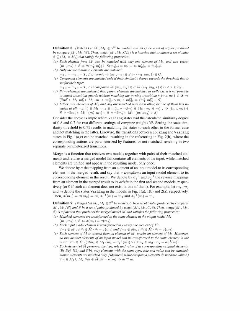
Definition 8. (Match) Let M1,M2 ∈ 2M be models and let C be a set of triples producedby compare(M1,M2,W). Then, match(M1,M2, C, S) is a function that produces a set of pairsS ⊆ (M1 ×M2) that satisfy the following properties:(a) Each element from M1 can be matched with only one element of M2, and vice versa:

(m1,m2) ∈ S ⇒ ∀(m′1,m′2) ∈ S(m′1|id = m1|id ⇔ m′2|id = m2|id).(b) Only identical atomic elements are matched:

m1|t = m2|t = T , T is atomic⇒ (m1,m2) ∈ S ⇔ (m1,m2, 1) ∈ C.(c) Compound elements are matched only if their similarity degree exceeds the threshold that is

set for their type:m1|t = m2|t = T , T is compound⇒ (m1,m2) ∈ S ⇔ (m1,m2, x) ∈ C ∧ x ≥ ST .

(d) If two elements are matched, their parent elements are matched as well (e.g., it is not possibleto match transition guards without matching the owning transitions): (m1,m2) ∈ S ⇒(∃mp

1 ∈M1,mp2 ∈M2 ·m1 ∈ mp

1|s ∧m2 ∈ mp2|s ⇒ (mp

1,mp2) ∈ S).

(e) Either root elements of M1 and M2 are matched with each other, or one of them has nomatch at all: ¬∃mp

1 ∈ M1 ·m1 ∈ mp1|s ∧ ¬∃m

p2 ∈ M2 ·m2 ∈ mp

2|s ⇒ ((m1,m2) ∈S ∨ ¬∃m′1 ∈M1 · (m′1,m2) ∈ S ∨ ¬∃m′2 ∈M2 · (m1,m

′2) ∈ S).

Consider the above example where Washing states had the calculated similarity degreeof 0.8 and 0.7 for two different settings of compare weights W. Setting the state sim-ilarity threshold to 0.75 results in matching the states to each other in the former caseand not matching in the latter. Likewise, the transitions between Locking and Washingstates in Fig. 1(a,c) can be matched, resulting in the refactoring in Fig. 2(b), where thecorresponding actions are parameterized by features, or not matched, resulting in twoseparate parameterized transitions.

Merge is a function that receives two models together with pairs of their matched ele-ments and returns a merged model that contains all elements of the input, while matchedelements are unified and appear in the resulting model only once.

We denote by σ the mapping from an element of an input model to its correspondingelement in the merged result, and say that σ transforms an input model element to itscorresponding element in the result. We denote by σ−11 and σ−12 the reverse mappingsfrom an element in the merged result to its origin in the first and second models, respec-tively (or ∅ if such an element does not exist in one of them). For example, let m1, m2

and m denote the states Washing in the models in Fig. 1(a), 1(b) and 2(a), respectively.Then, σ(m1) = σ(m2) = m, σ−11 (m) = m1 and σ−12 (m) = m2.

Definition 9. (Merge) LetM1,M2 ∈ 2M be models,C be a set of triples produced by compare(M1,M2,W) and S be a set of pairs produced by match(M1,M2, C, S). Then, merge(M1,M2,S) is a function that produces the merged model M and satisfies the following properties:(a) Matched elements are transformed to the same element in the output model M :

(m1,m2) ∈ S ⇔ σ(m1) = σ(m2).(b) Each input model element is transformed to exactly one element of M :∀m1 ∈M1, ∃!m ∈ M · m = σ(m1) and ∀m2 ∈M2,∃!m ∈ M · m = σ(m2).

(c) Each element of M is created from an element of M1 and/or an element of M2. Moreover,no two distinct elements of an input model can be transformed to the same element in theresult: ∀m ∈ M · (∃!m1 ∈M1 ·m1 = σ−1

1 (m)) ∨ (∃!m2 ∈M2 ·m2 = σ−12 (m)).

(d) Each element of M preserves the type, role and value of its corresponding original elements.(By Def. 7(b) and 8(b), only elements with the same type, role and value can be matched:atomic elements are matched only if identical, while compound elements do not have values.)∀m ∈M1 ∪M2, ∀m ∈ M, m = σ(m)⇒ m ∼= m.

(e) Each element of M preserves sub-elements of its corresponding original elements:∀m ∈ M, mc ∈ m|s ⇔ (σ−1

1 (mc) ∈ σ−11 (m)|s) ∨ (σ−1

2 (mc) ∈ σ−12 (m)|s).

While the compare and match functions rely on heuristically set weights W and simi-larity degrees S, merge is not heuristic: its output is uniquely defined by the input set ofmatched elements. For this work, we rely on union-merge [22] realization of the mergefunction. Union-merge unifies matched elements and copies unmatched elements “asis” to the result. Since our data model in Sec. 2 represents attributes of model elementsas separate entities, an element in the merged result can have several attributes of thesame type fulfilling the same role (which, for example, is not allowed by UML foreffects on a transition or state do activities). We use this property of the data modelto capture annotative product line representations generated when merging individualproducts into product lines.

4 Product Line RefactoringIn this section, we define the merge-in operator, which is used to put together inputproducts into a product line. It constructs a product line by adding input products oneby one and has two parameters: an (already constructed) product line and the next modelto add2. For the example in Fig 1, combining Controller A and B in Fig. 1(a,b) resultsin a product line A+B depicted in Fig. 2(a), with features fA and fB . Selecting the firstone derives the original statechart of Controller A, while selecting the second – thatof Controller B. Subsequent merge-in of Controller C (Fig. 1(c)) into this productline produces a representation depicted in Fig. 2(b), out of which all three originalstatecharts can be derived.

Definition 10. (Merge-in Construction) PL′ = 〈FM′,M′,R′〉 is a product line constructedby merging-in a product M into the product line PL (denoted by PL′ = PL ⊕W,S M ), usingthe rules below:(a) A new feature fM , representing the merged-in product M , is added as an alternative to all

existing features: if FM = 〈F , ϕ〉 then FM′ = 〈F ′, ϕ′〉, F ′ = F ∪ {fM |fM ∈ F,fM 6∈ F}, and ϕ′ = (ϕ ∨ fM ) ∧

∧f∈F¬(fM ∧ f).

(b) The domain model is generated by merging the existing domain model with the newly addedmodelM : ifC = compare(M,M,W) and S = match(M,M,C, S) thenM′ = merge(M,M, S).

(c) The set of annotation relationships is enhanced by the relationships that annotate elementsthat originated in M by fM : R′ = {(f, σ(m)) | f ∈ F ,m ∈ M, (f,m) ∈ R} ∪{(fM , σ(m)) |m ∈M}.

We refer to PL as the original product line and to PL′ as the constructed product line.

5 Correctness of Product Line RefactoringIn this section, we prove the correctness of the merge-in operator introduced in Sec. 4.Specifically, we show that merge-in produces minimal behavior-preserving product linerefinements [2], that is, the input product models are the only ones which can be derivedfrom the refactored product line model (Theorem 1).

2 The first product is implicitly converted into a “primitive” product line – a product line withonly one feature and a set of annotations that relate all model elements to that feature.

In what follows, let W be a set of weights used by the compare function and S be aset of similarity thresholds used by the match functions. Let PL = 〈FM,M,R〉 be aproduct line.Merge-in Monotonicity. Lemma 2 below shows that any feature configuration that con-tains only features from the original product linePL is also a valid feature configurationfor the constructed product line PL′, i.e., it complies to the constrains ϕ defined on thefeatures of PL′. For the example in Fig. 2, this means that a feature configuration ofthe product line A+B in Fig. 2(a), e.g., {fA}, is also a valid feature configuration forthe “extended” product line A+B+C in Fig. 2(b).

Lemma 2. Let FM be a subset of FM. Then, FM is a feature configuration of FM if andonly if it is a feature configuration of FM′.

Proof. By construction of ϕ′ (Def. 10(a)), ϕ′ = (ϕ∨fM )∧∧

f∈F¬(fM ∧f). Since fM 6∈ FM,

¬(fM ∧ f) evaluates to true for every f , and ϕ′ = (ϕ ∨ false) = ϕ. Thus, FM respects ϕ ifand only if it respects ϕ′.

Lemma 3 shows that, under configurations used in Lemma 2, a model derived fromPL is equal to the one derived from PL′. That is, under the configuration {fA}, thesame model of ControllerA in Fig. 1(a) is derived from both product lines A+B andA+B+C (Fig. 2(a) and (b), respectively).

Lemma 3. Let FM be a subset of FM. If FM is a feature configuration for FM, M =

∆(PL, FM) and M ′ = ∆(PL′, FM), then M = M ′. That is, given a feature configurationthat contains only features from PL, a set of elements that is generated from PL is equivalent tothat generated from PL′, under the same configuration.

Proof. To prove the lemma, we show that f = ∆(σ(∆−1(.))) is an isomorphism between theelements of M and the elements of M ′ that respects ∼=. That is, we prove the following fourstatements, showing that f is an edge-preserving bijection. The construction of the correspond-ing elements in M and M ′ is schematically sketched in Fig. 4.

1. Any element of M has the corresponding equal element in M ′: ∀m ∈ M, ∃!m′ ∈M ′ · m′ = f(m) ∧ m′ ∼= m.Let m ∈ M . By Def. 6(a), this means that there exists an element m ∈ M, and a featuref ∈ FM, such that (f,m) ∈ R and m = ∆(m). By Def. 9(b), m is transformed by mergeto an element m′ ∈ M′, such that m′ = σ(m). By Def. 10(c), this element is annotated by thesame feature as m: (f, σ(m)) ∈ R′. Thus, ∆(σ(m)) ∈ M by Def. 6(a). Since m is derivedfromm,m = ∆−1(m). It follows that∆(σ(∆−1(m))) ∈ M ′. Let’s denote that element by m′.There exists only one such element by Def. 6(b,c) and 9(b). m′ ∼= m by Def. 6(d) and 9(d).

2. Any element of M ′ has the corresponding equal element in M : ∀m′ ∈ M ′,∃!m ∈M · m′ = f(m) ∧ m′ ∼= m.Let m′ ∈ M ′. By Def. 6(a), this means that there exist an element m′ ∈ M′, and a featuref ∈ FM, such that (f, m′) ∈ R′ and m′ = ∆(m′). By Def. 9(c), there are three possiblecases: (1) σ−1

1 (m′) ∈M, σ−12 (m′) = ∅; (2) σ−1

1 (m′) = ∅, σ−12 (m′) ∈M ; (3) σ−1

1 (m′) ∈M,σ−12 (m′) ∈M .

For cases (1) and (3), (f, m′) ∈ R′ implies that (f, σ−11 (m′)) ∈ R by Def. 10(c), and thus,

∆(σ−11 (m′)) ∈ M by Def. 6(a). Let’s denote this element by m. It is easy to see that f(m) = m′

(that is ∆(σ(∆−1(m))) = m′. There exists only one such element m by Def. 6(b,c) and 9(c).m′ ∼= m by Def. 6(d) and 9(d). For case (2), σ−1

1 (m′) = ∅ implies by Def. 10(c), that m′ isannotated by fM , and, since fM 6∈ FM, ∆(m′) 6∈ M ′, which, together with m′ = ∆(m′),

creates a contradiction to m′ ∈ M ′.3. Any sub-element of m has the corresponding sub-element in f(m): ∀m ∈ M(mc ∈

m|s ⇒ f(mc) ∈ f(m)|s).Since mc ∈ m|s, by Def. 6(a,e), there exist elements m,mc ∈ M, and features f, fc ∈ FM,such that (f,m) ∈ R, (fc,mc) ∈ R, m = ∆(m), mc = ∆(mc) and mc ∈ m|s (it isalso possible that f = fc). By Def. 9(b,e), σ(mc) ∈ σ(m)|s. By Def. 10(c), (f, σ(m)) ∈ R′and (fc, σ(mc)) ∈ R′, which, by Def. 6(a,e), implies that ∆(σ(mc)) ∈ ∆(σ(m))|s. Sincemc = ∆−1(mc) and m = ∆−1(m), f(mc) ∈ f(m)|s), as desired.

4. Any sub-element of m′ has the corresponding sub-element in m: ∀m′ ∈ M ′(m′c ∈m′|s ⇒ ∃m, mc ∈ M · m′ = f(m) ∧ m′c = f(mc) ∧ mc ∈ m|s.Let m′c, m′ ∈ M ′ be elements such that m′c ∈ m′|s. By Def. 6(a,e), there exist elementsm′, m′c ∈ M′, and features f, fc ∈ FM, such that (f, m′) ∈ R′, (fc, m′c) ∈ R′, m′ =∆(m′), m′c = ∆(m′c) and m′c ∈ m′|s (it is also possible that f = fc). Similarly to case 2,σ−11 (m′) 6= ∅ and σ−1

1 (m′c) 6= ∅. By Def. 9(e), either σ−11 (m′c) ∈ σ−1

1 (m′)|s or there existm1,m2 ∈M , such that σ−1

1 (m′c) is matched withm1, σ−11 (m′) is matched withm2, andm1 ∈

m2|s. The later case is impossible by Def. 8(a,d,e) – we omit the details due to the space limita-tions. For the former case, since (f, m′) ∈ R′, (fc, m′c) ∈ R′, by Def. 10(c), (f, σ−1

1 (m′)) ∈R, (fc, σ−1

1 (m′c)) ∈ R and thus, by Def. 6(a,e), ∆(σ−11 (m′c))) ∈ ∆(σ−1

1 (m′)))|s. Let’sdenote these elements by mc and m, respectively. f(mc)) = ∆(m′c) = m′c and f(m)) =∆(m′) = m′, implies mc ∈ m|s, as desired.

Fig. 4. A sketch for the proof of Lemma 3.

The above lemma implies thatour construction preserves the be-havior of the original product linemodel: the set of models derivedfrom PL can still be derived fromPL′, as shown by the followingcorollary.

Corollary 1. Let bPLc denote a setof all models derived from a prod-uct line PL. That is, bPLc =

{∆(PL, FM) | FM is a feature configuration of FM}. Then, a set of models de-rived from PL can be derived from PL′ as well: bPLc ⊆ bPL′c.Proof. For each M ∈ bPLc, there exists a configuration FM, such that M = ∆(PL, FM).By Lemmas 2 and 3, M = ∆(PL′, FM). Thus, M ∈ bPL′c.For the example in Fig. 2, the above corollary means that both Controller A andController B that can be derived from the product line A+B in Fig. 2(a) can still bederived from the constructed product line A+B+C in Fig. 2(b), after Controller Cwas merged-in to it.Merge-in Behavior Preservation. We now show that model M which we merge-ininto the original product line PL can be derived from the constructed product line PL′.That is, when we merge-in Controller C in Fig. 1(c) into the product line A+B inFig. 2(a), we can derive it back from the constructed product line A+B+C in Fig. 2(b).

Since fM is the feature that annotates elements of the merged-in model (fC in ourexample), we first show that {fM} is a valid feature configuration (Lemma 4). Then,Lemma 5 shows that the original model M is derived from the constructed product linePL′ under that configuration.

Lemma 4. {fM} is a feature configuration for PL′.

Proof. By construction of FM′ (Def. 10(a)), fM ∈ F ′. We now show that {fM}respects ϕ′ = (ϕ∨ fM )∧

∧f∈F¬(fM ∧ f). Since f 6∈ {fM} for any f ∈ F , ¬(fM ∧ f)

evaluates to true for every f ∈ F . Since fM = true, ϕ ∨ fM also evaluated to true. Itfollows that {fM} respects ϕ′ and is a feature configuration for PL′.

Lemma 5. Let {fM} be a feature configuration. Then, a model that is derived from PL′ underthat configuration is equivalent to M . That is, M = ∆(PL′, {fM}).

The proof of this lemma, similarly to the proof of Lemma 3, shows that f = σ(∆(.)) isan isomorphism between the elements of M and the elements of M ′, and is omitted.

Finally, Theorem 1 shows that our merge-in operator is behavior preserving: the setof product models that are derived from the constructed product line PL′ is equal tothe set of models that are derived from the original product line PL′, in addition to themerged-in model M .

Theorem 1. bPL′c = bPLc ∪ {M}.

Proof. We first prove that bPL′c ⊆ bPLc ∪ {M}. Let M ∈ bPL′c be a model derived fromPL′. Then there exists a feature configuration FM

′, such that M = ∆(PL′, FM

′). Let fM be

in FM′ r FM.1. If fM 6∈ FM

′, then FM

′⊆ FM. Thus, by Lemma 3, M = ∆(PL, FM

′), which

implies that M ∈ bPLc.2. If fM ∈ FM

′, then, by construction of FM′ (Def. 10(a)), FM

′= {fM}. By Lemma 5,

M = ∆(PL′, FM′). Thus, by Lemma 1, M = M .

We now show that bPLc∪ {M} ⊆ bPL′c. bPLc ⊆ bPL′c by Corollary 1. By the constructionof FM′ (Def. 10(a)), fM ∈ F ′. Thus, by Lemmas 4 and 5, {fM} is a valid feature configurationfor PL′ and M = ∆(PL′, {fM}), which implies that M ∈ bPL′c.

For the example in Fig. 2, where Controller C in Fig. 1(c) is merged-in into theproduct line A+B containing Controller A and B, this means that Controller A,B, and C, and only them, can be derived from the constructed product line A+B+C inFig. 2(b).

6 Related WorkA general theory of product line refinement was introduced in [2] where the authorsestablished product line properties supporting stepwise and compositional product linedevelopment and evolution. Our approach instantiates this theory by providing a con-crete refactoring technique for combining products into product lines. We prove thatour refactoring is the minimal behavior-preserving product line refinement, accordingto the definition in [2].

Several works (e.g., [9, 10]) capture guidelines and techniques for manually trans-forming legacy product line artifacts into SPLE representations. Instead, our goal is tointroduce automation into the refactoring process by comparing, matching and mergingartifacts to each other. While no automated approach can replace a human product line

designer and produce a solution which is as good as a hand-crafted one, automation canassist the designer and speed-up the refactoring process.

Similarly to us, Koschke et. al. [11] and Ryssel et. al. [21] introduce automaticapproaches to re-organize product variants into annotative representations while identi-fying variation points and their dependencies. The former work reasons about compo-nents, interfaces and their grouping into subsystems. The latter works on Matlab mod-els. Our work differs from both [11] and [21] by exploring product line commonalitiesand variabilities for any type of model that can be represented as XMI and by providinga formal proof of correctness of our approach.

Feature-oriented refactoring [13, 15] focuses on identifying the code for a featureand factoring the code out into a single module or aspect aiming at decomposing a pro-gram into features. Since our aim is consolidation of variants into single-base productline representations, these are out of the scope for our work. Similarly, UML modelrefactoring (e.g., [6, 24]) and code refactoring techniques (e.g., [14]), while closely re-lated to our work, usually focus on improving the internal structure and design of asoftware system rather than on identifying and restructuring the system’s common andvariable parts.

7 Conclusion and Future Work

Extracting product line representations from existing legacy product line systems cansupport product line engineering adoption: reusing and leveraging knowledge accumu-lated in the legacy systems during their development lifetime can be more efficient than“starting from scratch”. In this work, we formally specified a simple data model and arefactoring technique for transforming individual products into more compact productline representations. Our data model, inspired by XMI principles, is powerful enoughto accommodate labeled-graph representations, in particular, UML. At the same time, itis flexible enough to support product line notations where several alternative elementscan fulfill the same role, which is not allowed by UML itself.

Relying on the data model, we formally stated necessary and sufficient conditionsallowing us to use model compare, match and merge operators for combining individ-ual products into product lines. We proved that once these conditions are satisfied, themerge-in can be safely applied for combining products into product lines, as it producesrepresentations that encode precisely the set of initial products. This provides formalfoundation that underlays the parameterizable and configurable, yet semantically cor-rect refactoring framework. The applicability of the framework to real-life examples, aswell as techniques for distinguishing between different possible refactorings, is studiedelsewhere [20].

There are several directions for continuing this work. First, we are interested inexploring more sophisticated refactoring techniques that are able to detect fine-grainedfeatures in the combined products. This would allow us to create new products in theproduct line by “mixing” features from different original products. We also plan toenhance model merging techniques with additional capabilities, such as using code-level clone detection techniques for comparing statechart actions and activities. We arealso interested in devising alternative methods of calculating graph similarity, e.g., bycounting the number of identical or similar sub-graphs and more.

References

1. D. Beuche. Transforming Legacy Systems into Software Product Lines. In Proc. of SPLC’11Tutorial, 2011.

2. P. Borba, L. Teixeira, and R. Gheyi. A Theory of Software Product Line Refinement. InProc. of ICTAC’10, pages 15–43, 2010.

3. Q. Boucher, A. Classen, P. Heymans, A. Bourdoux, and L. Demonceau. Tag and Prune: aPragmatic Approach to Software Product Line Implementation. In Proc. of ASE’10, 2010.

4. P. C. Clements and L. Northrop. Software Product Lines: Practices and Patterns. SEI Seriesin Software Engineering. Addison-Wesley, 2001.

5. H. Gomaa. Designing Software Product Lines with UML: From Use Cases to Pattern-BasedSoftware Architectures. Addison Wesley, 2004.

6. S. Hosseini and M. A. Azgomi. UML Model Refactoring with Emphasis on Behavior Preser-vation. In Proc. of TASE’08, pages 125–128, 2008.

7. K. Kang, S. Cohen, J. Hess, W. Nowak, and S. Peterson. Feature-Oriented Domain Analysis(FODA) Feasibility Study. Technical report, CMU/SEI-90TR-21, 1990.

8. C. Kastner and S. Apel. Integrating Compositional and Annotative Approaches for ProductLine Engineering. In Proc. of GPCE Wrksp. on Modul., Comp. and Gen. Tech. for PLE(GPLE’08), pages 35–40, 2008.

9. K. Kim, H. Kim, and W. Kim. Building Software Product Line from the Legacy Systems:Experience in the Digital Audio and Video Domain. In Proc. of SPLC’07, 2007.

10. R. Kolb, D. Muthig, T. Patzke, and K. Yamauchi. Refactoring a Legacy Component for Reusein a Software Product Line: a Case Study: Practice Articles. J. of Software Maintenance andEvolution, 18(2):109–132, 2006.

11. R. Koschke, P. Frenzel, A. P. Breu, and K. Angstmann. Extending the Reflection Method forConsolidating Software Variants into Product Lines. Soft. Quality Control, 17(4), 2009.

12. C. W. Krueger. Easing the Transition to Software Mass Customization. In Proc. of 4thWrksp. on Soft. Product-Family Eng. (PFE), pages 282–293. Springer-Verlag, 2002.

13. J. Liu, D. Batory, and C. Lengauer. Feature Oriented Refactoring of Legacy Applications. InProc. of ICSE’06, pages 112–121, 2006.

14. T. Mens and T. Tourwe. A Survey of Software Refactoring. IEEE TSE, 30(2):126–139, 2004.15. G. C. Murphy, A. Lai, R. J. Walker, and M. P. Robillard. Separating Features in Source Code:

an Exploratory Study. In Proc. of ICSE’01, pages 275–284, 2001.16. S. Nejati, M. Sabetzadeh, M. Chechik, S. Easterbrook, and P. Zave. Matching and Merging

of Statecharts Specifications. In Proc. of ICSE’07, pages 54–64, 2007.17. OMG. http://www.omg.org/spec/XMI/2.1.1/. Last Accessed: January 2011.18. K. Pohl, F. Guenter Boeckle, and van der Linden. Software Product Line Engineering: Foun-

dations, Principles, and Techniques. Springer, 2005.19. J. Rubin and M. Chechik. From Products to Product Lines Using Model Matching and

Refactoring. In Proc. of SPLC Wrksp. (MAPLE’10), 2010.20. J. Rubin and M. Chechik. Quality of Behavior-Preserving Product Line Refactorings, 2011.

Under review.21. U. Ryssel, J. Ploennigs, and K. Kabitzsch. Extraction of Feature Models from Formal Con-

texts. In Proc. of SPLC’11, pages 4:1–4:8, 2011.22. M. Sabetzadeh and S. Easterbrook. View Merging in the Presence of Incompleteness and

Inconsistency. Requirement Engineering, 11:174–193, June 2006.23. S. She, R. Lotufo, T. Berger, A. Wasowski, and K. Czarnecki. Reverse Engineering Feature

Models. In Proc. of ICSE’11, 2011.24. G. Sunye, D. Pollet, Y. L. Traon, and J.-M. Jezequel. Refactoring UML Models. In Proc. of

UML’01, pages 134–148, 2001.

combining related products into product lineschechik/pubs/fase12.pdf · combining related products...

Documents