combining quantitative and logical data...
TRANSCRIPT

Combining Quantitative and Logical Data Cleaning
Nataliya Prokoshyna∗
Dept. of Computer ScienceUniversity of Toronto
Jaroslaw Szlichta*University of Ontario
Institute of [email protected]
Fei ChiangDept. of Computing and Software
McMaster [email protected]
Renee J. Miller*CS, University of Toronto
Divesh SrivastavaAT&T Labs Research
ABSTRACTQuantitative data cleaning relies on the use of statisticalmethods to identify and repair data quality problems whilelogical data cleaning tackles the same problems using vari-ous forms of logical reasoning over declarative dependencies.Each of these approaches has its strengths: the logical ap-proach is able to capture subtle data quality problems usingsophisticated dependencies, while the quantitative approachexcels at ensuring that the repaired data has desired statisti-cal properties. We propose a novel framework within whichthese two approaches can be used synergistically to combinetheir respective strengths.
We instantiate our framework using (i) metric functionaldependencies (metric FDs), a type of dependency that gen-eralizes the commonly used FDs to identify inconsistenciesin domains where only large differences in metric data areconsidered to be a data quality problem, and (ii) repairsthat modify the inconsistent data so as to minimize sta-tistical distortion, measured using the Earth Mover’s Dis-tance (EMD). We show that the problem of computing astatistical distortion minimal repair is NP-hard. Given thiscomplexity, we present an efficient algorithm for finding aminimal repair that has a small statistical distortion usingEMD computation over semantically related attributes. Toidentify semantically related attributes, we present a soundand complete axiomatization and an efficient algorithm fortesting implication of metric FDs. While the complexity ofinference for some other FD extensions is co-NP complete,we show that the inference problem for metric FDs remainslinear, as in traditional FDs. We prove that every instancethat can be generated by our repair algorithm is set mini-mal (with no redundant changes). Our experimental evalua-tion demonstrates that our techniques obtain a considerablylower statistical distortion than existing repair techniques,while achieving similar levels of efficiency.
∗Supported by NSERC BIN (and Szlichta by MITACS).
1. INTRODUCTIONTwo major trends in data cleaning have emerged. The
first is a logical approach to cleaning; the second a quan-titative or statistical one. In logical data cleaning, errordetection is typically performed using declarative cleaningprograms that specify data quality rules [13]. In constraint-based cleaning, data dependencies are used to specify qual-ity requirements. Cleaning, then, can take a form of logicalrules for correcting errors (for example, if a cleaning pro-gram asserts that a sensor should have a single reading atany time point, it may also contain a resolution strategythat replaces multiple readings with their average). Datathat is inconsistent with respect to the constraints can berepaired by finding a minimal set of changes that fix theerrors [7, 16]. An important advantage of such approachesis that they are able to find subtle data quality problemsusing sophisticated dependencies. Repair is typically donebased on minimizing the number or cost of changes neededto create a consistent database.
In quantitative data cleaning, there has been considerablework on outlier detection for quantitative data (both uni-variate and multivariate or relational data) [15]. This hasbeen complemented with work on pairing repair strategieswith detection which considers multiple types of errors (fordifferent types of data) [3]. An important insight in this lat-ter work is that the cleaned data should be of higher dataquality than the original uncleaned data. To quantify this,Berti-Equille et al. [3] propose cleaning techniques that en-sure the cleaned data is statistically close to an ideal dataset.Dasu and Loh [10] coined the term statistical distortion forthe distance between the distribution of a (cleaned) datasetand a user-defined ideal dataset. Both these papers proposestatistical distortion as a way to (post facto) evaluate (andcompare) different cleaning strategies. However, a quanti-tative repair is not guaranteed to be logically consistent.
There has, to date, been little work combining the in-sights of these two separate threads of research. Yakout etal. [26] propose a cleaning technique that separates detec-tion from repair. Detection may be done using clean masterdata, using constraints or using quantitative outlier detec-tion. Repair on the detected (potential) errors is done usingquantitative cleaning. However, unlike our approach theydo not make use of integrity constraints to obtain a finer-grained view of what data needs to be repaired, ensure therepair is a consistent database, or guarantee that only min-imal (necessary) changes are done.
1

In contrast, our technique comprehensively combines quan-titative and logical approaches. We propose a new constraint-based cleaning strategy in which we use statistical distortionduring cleaning to ensure the chosen (minimal) repair is ofas high quality as possible.
1.1 Cleaning ExampleConsider the relation in Table 1.1. The data is inte-
grated information about employees, their positions in or-ganizations, and the locations (latitude, longitude) of theorganizations, from multiple sources. For our data qualityconstraints, we make use of metric functional dependencies(metric FDs) [17]. Metric FDs generalize traditional FDs topermit some variation in the values of attributes that ap-pear in their consequent. They are appropriate in domainswhere only a large variation in values indicates a real seman-tic difference. In each of the three dependencies (Table 1.1),the value of θ indicates how much variation is permitted.For values in the Latitude and Longitude attributes, weuse a metric that is the difference in degrees; θ = 0.01 isapproximately 1km. For values in the Organization at-tribute, we use a metric that is an edit distance (θ = 6); forexample, an edit distance between Univ of Toronto andUniversity of Toronto is six, therefore these two valuessatisfy the threshold. Additionally, we assume a preprocess-ing step is performed that takes into account organizationalsynonyms. Since AT&T Labs Research and Shannon Labs
are synonyms we use their canonical name, for instance,AT&T Labs Research (Section 2.1).
The metric FD M1 indicates that if two tuples share thesame Person and Position values, then the edit distancebetween their Organization values should be 6 (indicatedby the θ = 6 in Table 1.1); this variation may be permit-ted due to conventions in different sources. Assuming thatAT&T Labs Research and Shannon Labs are synonyms witha canonical name AT&T Labs Research, then normalized tu-ples t8 and t9 (and our entire example relation) satisfy M1.
The metric FDs M2 and M3 indicate that if two tuplesshare the same Organization value (i.e., their distance is0), then their Latitude and Longitude values, respectively,should differ by no more than 0.01 degree; this variation maybe permitted due to differences in GPS measurements orin conventions about the exact location of an organization.Hence, tuples t6 and t7 together satisfy these dependencies,as do tuples t8 and t9, while t1 and t2 do not.
Consider a purely logical approach to cleaning, using aminimal repair. There are different notions of minimalityin the literature, but for illustration, consider only modifi-cations of attribute values (i.e., no deletion or insertion oftuples). A repair is minimal if we cannot undo any mod-ification and still have a relation that is consistent; as weexplain in Section 2, this is called set-minimal repair [5].
Consider repairing the inconsistencies on metric FDs M2andM3 among tuples for the organization Univ of Toronto
(namely, t1, t2, t4, t6 and t7). A set-minimal repair couldchange the Latitude values of t2 and t4 to be within 0.01degrees of both 43.66 and 43.662892, and the Longitude val-ues of t2 and t4 to be within 0.01 degrees of both −79.395656and −79.40. But set-minimality does not tell us which val-ues in these ranges to pick. We could use a measure likesupport [8] to change a value to the most frequent value(in this case, 43.662892 for Latitude and −79.395656 forLongitude). Or we could use Winsorization [10] to change
a value to the closest value that is consistent with the othertuples (in this case, both the Latitude values −33.0142425in t2 and 40.4587165 in t4 would change to 43.66). However,such approaches can lead to statistical drift, with frequentvalues being overly represented in the cleaned relation, oroutlier erroneous values (like −33.0142425) pulling the datadistribution too far in the direction of the outliers.
Alternatively, we could change the Organization of t2and t4 to be different from that of t1, t6, t7. This changewould be minimal as well, and would involve changing onlytwo attribute values instead of four values as in the case ofchanging Latitude and Longitude values of t2 and t4. Butwhich repair is better? And what values (in the specifiedranges) should we pick for the repairs? Some approaches usemeasures like support or co-occurrence of values within thedirty relation itself to pick among alternate minimal repairs.We propose instead to pick a repair that minimizes statisticaldistortion with respect to an ideal relation [10, 3, 26].
To illustrate why the strategy to minimize statistical dis-tortion can be desirable, consider M2 and M3 in our ex-ample. Instead of creating a potential statistical bias byrepairing the Latitude and Longitude values of t2 and t4to the most frequent or the closest values, or changing theOrganization values of t2 and t4 to some different values,our approach will use the ideal relation (Section 2) as aguide, and pick repair values so as to mimic the ideal distri-bution as close as possible.
Most existing repair approaches use a notion of minimal-ity (minimizing the number of changes) [5] or minimal costrepair [4, 7, 16] to decide on values to use in repairing errors.Their objective function is based on the number or cost ofrepairs with respect to the original dirty dataset. Like theseexisting approaches, we could define DI as the original dirtydataset. The difference would be the objective function –they minimize counts or cost (where cost is defined with re-spect to a distance function over attribute values), while weminimize statistical distortion. A benefit of our approachhowever (one that has been observed by others [3, 10, 26]) isthat we have freedom in defining DI . It can be the originaldirty data or it can be a clean subset of the data. A usercan decide if the evidence they want to use in cleaning isbest captured by the original data, or only the data withoutthe errors (since these errors may change the distribution).Alternatively, and most realistically, in a continuous datacleaning process [24], a user can use a previously cleanedand verified dataset as DI .
Our approach is applicable for applications where errorsare introduced in a relatively independent manner and theamount of errors remains small relative to the data size orto a previously cleaned DI . Such datasets are commonin practice (e.g., sensor based appli- cations, flight arrivaltimes, GPS transit tracking) where unexpected events (e.g.,dropped data or delays) can lead to errors, but the data isexpected to conform to a (known) distribution of expectedevents. In contrast, when errors are introduced systemati-cally, for example by a faulty information-extraction process,then other approaches, like the Data X-Ray [25], are moreappropriate than ours.
In our example, if the ideal relation is the user-specifiedset of tuples t1, t3, t5, t6, t7, t8 and t9 (which in this case is amaximal consistent subset of the dirty data), the distribu-tions of values for Organization, Latitude and Longitude
in the ideal relation leads to a repair of t2, t4 and t10 shown in
2

TID Source Person Position Organization Latitude Longitude
t1 S2 NP Student Univ of Toronto 43.662892 -79.395656t2 S3 JS Student University of Toronto -33.0142425 151.5818976t3 S2 JS Faculty UOIT 43.943445 -78.895452t4 S3 FC Student Univ of Toronto 40.4587165 -80.6088795t5 S2 FC Faculty McMaster Univ 43.260879 -79.919225t6 S2 RJM Faculty Univ of Toronto 43.662892 -79.395656t7 S1 RJM Faculty Univ of Toronto 43.66 -79.40t8 S2 DS Manager AT&T Labs Research 40.669550 -74.636399t9 S1 DS Manager Shannon Labs 40.67 -74.63t10 S3 DS Manager AT&T Labs Research 30.391161 -97.751548
M1: Person, Position 7→ Organization (θ = 6) M2: Organization 7→ Latitude (θ = 0.01) M3: Organization 7→ Longitude (θ = 0.01)
Table 1.1: A dirty relation & data quality constraints.
TID Source Person Position Organization Latitude Longitude
t′2 S3 JS Student Univ of Toronto 43.66 -79.40t′4 S3 FC Student Univ of Toronto 43.662892 -79.395656t′10 S3 DS Manager AT&T Labs Research 40.669550 -74.636399
Table 1.2: Repaired tuples.
Table 1.2. Note that distributions of attribute values in thecleaned relation t1, t
′2, t3, t
′4, t5, t6, t7, t8, t9, t
′10 is statistically
closer or equal to the ideal relation than other modification-only repairs that could be performed.
1.2 Contributions• A new framework that combines the benefits oflogical and quantitative data cleaning. A statistical-distortion minimal repair is a consistent relation that bothdiffers set-minimally from the original dirty relation and thatdiffers minimally, in terms of statistical distortion from anideal relation. We have chosen to use metric FDs (a strictsuperset of FDs) to capture data quality requirements, be-cause of their importance in representing the semantics ofintegrated data (where small differences in a quantitativeattribute may not indicate a semantic difference). We usemetric FDs to identify errors in the data, and we proposestatistical repairs to resolve these errors.• An algorithm that efficiently and effectively com-putes a set-minimal repair with low statistical dis-tortion. We present that the problem of computing statis-tical distortion minimal repairs is NP-hard. Our algorithmuses the Earth Mover’s Distance (EMD) to calculate thestatistical distortion. Computing the EMD is well-known tobe computationally expensive [18, 19]. Hence, we proposeseveral optimizations via sampling that significantly improvethe performance of our algorithm without compromising thequality of our repairs. These include a pruning strategy thatremoves low frequency values (at the tail of the distribution)to reduce the search space of repairs since these values areunlikely to be chosen in a statistical repair.• The foundations of how metric FDs can be usedfor data cleaning. While FDs and extensions includingconditional FDs [6] and matching dependencies [11] havebeen used extensively for data cleaning, ours is the first ap-plication of metric FDs to cleaning. To permit their usein cleaning, we must understand the inference problem formetric FDs. To this end, we present a sound and completeaxiomatization for metric FDs. While the complexity of in-ference for some other FD extensions with various notions ofsimilarity instead of strict equality, called differential depen-dencies [21], is co-NP-complete, we show that interestinglythe inference problem for metric FDs remains linear, as intraditional FDs. Our cleaning solution includes an imple-
mentation of our inference algorithm to compute the mini-mal cover of a set of metric FDs, and the closure of a set ofattributes under a set of metric FDs. As an optimization,our algorithm computes EMD only over attribute closuresrather than over the whole relation. We experimentally ver-ified that our inference system is efficient in practice.• An experimental evaluation showing the perfor-mance and effectiveness of our techniques using realand synthetic data. We experiment with different er-ror injection strategies (resulting in different relational datadistributions), and show that our framework achieves smallstatistical distortion when compared against an ideal datadistribution. Finally, we show that our algorithm is able toachieve improved (lower) statistical distortion over a recentlogical data repair solution [8].
Outline. We begin in Section 2 with a problem statementand a discussion of how logical and statistical data cleaningcan be combined. In Section 3, we present our repair algo-rithm that combines logical and statistical approaches. InSection 4, we provide logical foundations including an ax-iomatization and an inference procedure for metric FDs. Weexperimentally evaluate our techniques in Section 5. In Sec-tion 6, we discuss related work, and conclude in Section 7.
2. PROBLEM DEFINITIONTo combine logical and quantitative data cleaning, we will
use a set of constraints M to both identify errors and todefine a space of possible corrections (repairs). Followingcommon practice in quantitative data cleaning [10, 3, 26],we make use of an ideal distribution. We use DI to measurethe quality of a repair, that is, how well a repair preservesthe desired distribution of the data. Abstractly, we use thefollowing problem definition.Problem Definition Given a set of constraintsM , a datasetD where D 6|= M , and a dataset reflecting the desired datadistribution DI , find a repair Dr where Dr |= M and thestatistical distortion between Dr and DI is minimized.
We now give the specifics of the constraint language weconsider, the class of repairs, and how we will measure dis-tance between two relations.
2.1 Logical FoundationsTo begin, our constraint language will include functional
dependencies (FDs), the most common constraint used in
3

Table 2.1: Notational conventions.
• A bold capital letter represents a relation schema: R.• Italic capital letters near the beginning of the alphabet
represent single attributes: A, B and C.• A capital letter D in italic represents a relation.• Small italic letters near the end of the alphabet denote
tuples: s and t.• Small italic letters near the beginning of the alphabet
denote attribute values: a, b and c.• A small italic letter m denotes a similarity metric.• Italic capital letters near the end of alphabet stand for
sets of attributes: X, Y and Z.• XY is shorthand for X ∪ Y . Likewise, AX or XA stand
for X ∪ {A} and {} denotes an empty set.
data cleaning. In addition, we have chosen to consider met-ric functional dependencies, a strict superset of FDs [17].While the verification problem (determining if D |= M), formetric FDs has been studied, their use in data cleaning toguide data repair has not been studied. Metric FDs use asimilarity metric m that we define next.
Let R be a relation schema containing a set of attributes.For each attribute A ∈ R with domain dom(A), we assumethere is metric m : dom(A) × dom(A) → R. We use thismetric together with a threshold θ to define a similarityoperator over A.
Definition 2.1. (similarity operator)For every attribute A in a relational schema R assume abinary similarity relation (≈m,θ) wrt some similarity met-ric m and threshold parameter θ ≥ 0. For two tuples s andt, s[A] ≈m,θ t[A] iff m(s[A], t[A]) ≤ θ. Metric m satis-fies standard properties: symmetry, triangle inequality andidentity of indiscernibles (m(a, b) = 0 iff a = b)). For twotuples s, t in relation D over R we write s[X] ≈m, Θ t[X] tomean s[A1] ≈m1,θ1 t[A1], ..., s[An] ≈mn,θn t[An], where X= {A1, ..., An}, m = [m1, ..., mn] and Θ = [θ1, ..., θn].
A metric FD generalizes FDs to permit slight variationsin a functionally determined attribute. Note that if θ = 0then a metric FD is an FD.
Definition 2.2. (metric FD)Let X and Y be sets of attributes, mY and ΘY be metricsand thresholds for all the attributes in Y . Then, X 7→ Ydenotes a metric FD. A relation D satisfies X 7→ Y (D |=X 7→ Y ), iff for all tuples s, t ∈ D, s[X] = t[X] impliess[Y ] ≈mY ,ΘY t[Y ].
Metric FDs are defined over relations and throughout thispaper, we assume the dataset to be cleaned is a relation.
Example 2.3. Let D = {t1, ..., t10} from Table 1.1 andlet M = {M1,M2,M2}. As we argued in Section 1 D 6|= M ,more specifically M1 is satisfied, but M2 and M3 are not.However, if we remove t2, t4 and t10, then the remainingseven tuples do satisfy all constraints since the differencein Latitude and Longitude values for tuples with the sameOrganization is less than 0.01.
To permit attributes to contain synonyms (like the Orga-nization attribute in our running example), we assume thateach attribute value has a canonical name (in our example,AT&T Labs Research and Shannon Labs have a canonical
name AT&T Labs Research). Therefore, for any relation D,there is a function normalize(D) that replaces attribute val-ues with canonical names. So when we write D |= M , wemean normalize(D) |= M .
Definition 2.4. (consistent relation)Given M , a set of metric FDs, a relation D is consistent
iff D |= M . Otherwise, D is inconsistent (or dirty).
We define repairs using value modification only, that is,attribute values of a tuple may be changed but tuples maynot be inserted or deleted.
Definition 2.5. (repair)A repair of an inconsistent relation Dd is a consistent re-
lation Dr that can be created from Dd using a set of valuemodifications V.
Obviously, not all repairs are equally valuable. Changingthe value of every attribute to 1 in our running examplecreates a repair. But such a repair is intuitively less desir-able than the repair we depict in Table 1.2. Hence, thereare several well-know notions of minimal repairs for FDsthat are based on minimizing the number or cost of thechanges made to the data. A well-known notion of min-imality is cardinality-minimal repairs [5, 7, 16]. A repairis cardinality-minimal if the number of changes (|V|) is thesmallest possible among all possible repairs. A less restric-tive notion is set-minimal repairs. A repair Dr created by aset of value modifications is set-minimal if no subset of thechanged values in Dr can be reverted to their original valueswithout violating M [1, 5]. Cardinality-minimal repairs areset-minimal, but not vice versa.
Definition 2.6. (set-minimal repair)A repair Dr created by a set of changes V of an inconsistent
relation Dd is set-minimal iff there is no repair Dr′ that canbe created by a strict subset V ′ ⊂ V.
In set-minimal repairs, every change is necessary. Hence,the decision of whether to change a value is driven exclu-sively by the constraints. No value is changed unless it isnecessary to restore consistency. However, set-minimalityleaves some freedom (more freedom than cardinality-mini-mality) in selecting what values to use for modification, i.e.,how to repair. We will use statistical distortion to guide thischoice and decide which set-minimal repair to choose.
2.2 Statistical FoundationsWe assume a relation DI that follows the desired data
distribution. Given a set of candidate repairs, we will con-sider one repair better than another if it has lower statisticaldistortion from DI . Let MD(D) be the multi-dimensionaldistribution of a relation D.
Definition 2.7. (statistical distortion)Given relations D1 and D2, the statistical distortion (SD)
is defined as a distance between the distributions of D1 andD2, denoted as distance(MD(D1), MD(D2)).
For simplicity, we write distance(D1, D2) to mean dista-nce(MD(D1), MD(D2)). Following Dasu and Loh [10],to calculate the distance between distributions, we use theEarth Mover’s distance (EMD). EMD is a distance functionthat measures the dissimilarity of two histograms. In our
4

C11 = 0.0
wp1 = 2/3
p1 = 43.662892
p2 = 43.66
wp2 = 1/3
q1 = 43.662892
wq1 = 3/4
q2 = 43.66
wq1 = 1/4
C22 = 0.0
(a) Flow graph.
F11 = 2/3 p1 = 43.662892
p2 = 43.66
q1 = 43.662892
q2 = 43.66
F22 = 1/4
ssss
(b) Minimum cost flow.
Figure 2.1: The flow network.
work, this is based on the frequencies of the unique valuesin the dataset, often computed over a subset Z of the at-tributes in R. The set of bins in the histogram is the setof tuples in ΠZ(D). The weight, wpi , of a bin pi is therelative number of occurrences of this value in D (meaning|{t|ΠZ(t) = pi}| divided by |D|, where t is a tuple in D).
Definition 2.8. (Earth Mover’s Distance (EMD))Given two relational histograms, let P = {(p1, wp1), ...,
(pm, wpm)} and Q = {(q1, wq1), ..., (qn, wqn)}, each havingm and n bins respectively. Define a cost matrix C, where ci,jis a measure of dissimilarity between pi and qj, that modelsthe cost of transforming pi to qj, and a flow matrix F wherefi,j indicates the flow capacity between pi and qj. EMD isdefined in terms of an optimal flow that minimizes
d(P,Q) =
m∑i=1
n∑j=1
fij ∗ cij (1)
The EMD is defined as follows:
EMD(P,Q) = minF
d(P,Q) (2)
subject to the following constraints:
∀i ∈ [1,m],∀j ∈ [1, n] : fi,j ≥ 0,
∀i ∈ [1,m] :
n∑j=1
fi,j = wpi ,
∀j ∈ [1, n] :m∑i=1
fi,j = wqj ,
(3)
Equations 1-3 in Definition 2.8 are defined based on chang-ing the distribution of P to Q (and not vice versa) and limitthe amount of change that can be done to the bins in P andQ according to their respective weights. For two distribu-tions P and Q, EMD computes the distance between everyi-th bin in P and every j-th bin in Q. This is known as thecross-bin difference, and can be seen in Figure 2.1(a) wherean edge exists between every pair of nodes in the graph.Considering cross-bin differences makes EMD less sensitiveto the positioning of bin boundaries (note that a bin neednot contain only one value pi, but may in general containmany consecutive values).
Example 2.9. Continuing our example from Section 1,to compute EMD(P , Q), we compute the amount of work totransform P to Q. Let P = {t ∈ DI | ΠLat..(DI)}, whereDI = {t1, t6, t7}. Similarly, let Q = {t∈ DT | ΠLat.(DT )},where DT = {t1, t′4, t6, t7}, be the set of bins obtained bychanging the distribution from [ 2
3; 1
3] to [ 3
4; 1
4].
Figure 2.1(a) shows a graph representing P and Q, whereeach node represents a bin (e.g., bin p1 = ΠLat.(t1, t6)= 43.662892) along with their relative weights (wp1 = 2
3).
Let an edge weight cij be the absolute distance to trans-form pi to qj (e.g., c(1,2) = |43.662892 −43.66| = 0.002892).The best transformation (i.e., minimum flow between P andQ) is (0* 2
3) + (0.002892* 1
12) + (0* 1
4) = 0.000241 (Figure
2.1(b)).
We now define statistical-distortion minimal repair.
Definition 2.10. (statistical-distortion minimal repair)Given an ideal relation DI and a relation Dd that is incon-sistent with respect to a set of metric FDs M , a statistical-distortion (SD) minimal repair is a set-minimal repairDr for which EMD(Dr, DI) is minimal.
Despite the fact that we are relaxing minimality to con-sider set-minimal repairs which are easier to find than cardi-nality-minimal repairs (the problem of finding a cardinality-minimal repair for FDs is NP-hard [7, 16]), the problem offinding a SD minimal repair remains NP-hard.
Theorem 2.11. (complexity)The problem of finding a SD minimal repair is NP-hard.
In our proof [20], we show that for any set of FDs F overschema R, we can create (in polynomial time) a set of metricFDsM and function f such that Dr is a cardinality-minimalrepair for F iff f(Dr) is a statistical-distortion minimal re-pair of M. Hence, finding a statistical-distortion minimalrepair for a set of metric FDs is at least as hard as findinga cardinality-minimal repair for a set of FDs.
3. STATISTICAL REPAIR MODELWe propose a greedy algorithm that finds a maximal con-
sistent subset of a dirty relation Dd, and searches for a min-imal repair of each inconsistent tuple one at a time. Weselect among alternate tuple repairs by minimizing statis-tical distortion. We first discuss the main structure of thealgorithm, then discuss some additional ways of making thecomputation more efficient over large relations.
3.1 Algorithm for Generating RepairsLet Dd be a dirty relation and let Dc ⊂ Dd be a maximally
consistent set of tuples from Dd, meaning there is no tuplet ∈ Dd −Dc such that {t} ∪Dc is consistent. We call Du =Dd −Dc the unresolved data.
For each tuple td ∈ Du, we compute a set of possiblemodifications (tuple repairs). Each repair modifies attributevalues in td to create a candidate repaired tuple tr where{tr} ∪ Dc is consistent. Among the possible tuple repairsfor td, we select the tuple repair that minimizes statisticaldistortion from DI . To ensure we generate a set-minimalrepair, we ensure that tr is minimal, meaning that we can-not revert any value in tr to the value in td and still have atuple repair. Our algorithm assumes that the set of metricFDs M is a minimal cover meaning, among other things,that each constraint has the form X 7→ A (θA) where A is asingle attribute. Algorithms to compute a minimal cover forFDs are well-known. We show in Section 4 how to computea minimal cover for metric FDs. Note that our algorithm isgreedy. We repair tuples one at a time (without backtrack-ing) and minimize the distortion of the current clean subset.Of course, considering tuples in different orders (or usingdifferent maximally consistent subsets of tuples to start ouralgorithm) may lead to different repair choices. We empir-ically evaluate the influence of these choices on the quality
5

Algorithm 1 StatisticalDistRepair
Input: M (a minimal cover of a set of metric FDs),inconsistent relation Dd 6|= M , maximal clean subset Dc ⊆ Dd,ideal relation DIOutput: Repaired relation Dr of Dd1: Du = Dd −Dc (unresolved set)2: while Du 6= {} do3: select td ∈ Du; Du = Du − {td}4: M [td] = {m ∈M |{td} ∪Dc 6|= m} (deps violated by td)5: U = ∪X 7→A∈M [td]X (antecedents in violated deps)
6: V = ∪X 7→A∈M [td]A (consequents in violated deps)
7: Z = ∪XA ∈M (union of all attributes in M)8: Candidates = ∅ (find consequent repair candidates)9: for all v ∈ ΠV (σU=td[U ](Dc)) do
10: tv = td; tv [V ] = v11: if {tv} ∪Dc |= M then12: Candidates = Candidates ∪{tv}13: if Candidates 6= ∅ then14: tcons = argmint∈CandidatesEMD(t ∪Dc, DI)15: else16: tcons = ∅17: Candidates = ∅ (find antecedent repair candidates)18: for all u ∈ ΠU (V = σtd[V ](Dc))) do
19: tu = td; tu[U ] = u20: if {tu} ∪Dc |= M then21: Candidates = Candidates ∪{tu}22: if Candidates 6= ∅ then23: tante = argmint∈CandidatesEMD(t ∪Dc, DI)24: else25: tante = ∅26: if (tcons = ∅) ∧ (tante = ∅) then27: Candidates = k tuples in Dc closest to td[Z]28: tr = argmint∈CandidatesEMD(t ∪Dc, DI)29: else30: if (tante = ∅) ∨ (tcons 6= ∅ ∧ EMD(tcons ∪ Dc, DI) <
EMD(tante ∪Dc, DI)) then31: tr = tcons32: else33: tr = tante34: Dc = Dc ∪ { set-minimal(tr)}35: return Dr = Dc
of our solution in Section 5. Our algorithm is guaranteedto create a set-minimal repair and strives to minimize dis-tortion, but is not guaranteed to find a statistical-distortionminimal repair.
3.2 Tuple RepairsTo generate tuple repairs for a tuple td, we must consider
that td may violate many constraints in M . Let M [td] ={m ∈ M |{td} ∪ Dc 6|= m} be the set of dependencies thatwould be violated if td were added unmodified to Dc. LetU be the union of antecedents in M [td]. Let V be the unionof the consequents in M [td]. For each tuple, we first con-sider modifying attributes in V to create consequent-repairs(Lines 9-12 of Algorithm 1), then we consider modifyingattributes in U to create antecedent-repairs (Lines 18-21).For consequent-repairs, we consider modifying td[V ] (thetuple projected on the attributes of V ) to each value inΠV (U = σtd[U ](Dc)). Intuitively, this means that we re-pair the tuple to have the same consequent as some othertuple in Dc that shares its antecedent. This defines a setof candidate consequent-repairs. We keep only those repairstr such that {tr} ∪Dc |= M . We then compute the repairthat minimally distorts Dc among all these candidate repairs(argmintrEMD({tr} ∪ Dc, DI)). (Note in the rest of thepaper we omit set notation and write tr ∪Dc for simplicity.)
TID CEO Organization Longitude
t1 Stephenson AT&T -74.636399t2 Stephenson AT&T -74.636399t3 Stephenson IBM -97.751548
t′r Stephenson AT&T -97.751548t′′r Stephenson AT&T -74.636399
M1′: CEO 7→ Org (θ = 0) M2′: Org 7→ Longitude (θ = 1)
Table 3.1: Repairing both sides to satisfy constraints.
We do the same for antecedent-repairs. Specifically, weconsider modifying td[U ] to each value in ΠU (V = σtd[V ](Dc)).This defines a set of candidate antecedent-repairs. Again,we keep only those repairs tr such that tr ∪ Dc |= M andagain find one repair among these that minimally distortsDc from DI . If either a best consequent or a best antecedentrepair is found, we select the one with minimum distortion.Throughout, we break ties arbitrarily.
Example 3.1. Continuing our example from Section 1,Table 1.1, we may select the following maximally clean sub-set: Dc = {t1, t3, t5, t6, t7, t8, t9}. Suppose we select t4 as tdwhich violates M2 and M3. There are two possible consequent-repair candidates for t4, for each we would change only theLat and Long values of t4.
i) t′4[Lat, Long] = [43.662892, −79.395656] (uses t1, t6)
ii) t′′4 [Lat, Long] = [43.66,−79.40] (uses t7)
We choose the lower cost repair by computing EMD(t′4 ∪Dc, DI) and EMD(t4
′′∪Dc, DI). We also compute the set ofcandidate antecedent-repairs. Antecedent-repairs in this ex-ample change the Org value of t4 to be an organization that islocated at Lat =40.4587165 and Long = −80.6088795. How-ever, there are no such organizations in the clean dataset(no antecedent-repair candidates).
If we fail to find a valid antecedent or consequent-repair,then we consider modifying values in Z, where Z is all at-tributes in M (we call this a both-repair, see Lines 26–28 ofAlgorithm 1). Following the logic we used for other repairs,we could modify td[Z] to each value in ΠZ(Dc). However,this leads to a large number of candidate tuple repairs andthey will all be consistent wrt Dc. We limit this set tok tuples that are the closest to td (meaning the distancemZ(ΠZ(td),ΠZ(tr)) is minimum). Again, we keep the re-pair that minimally distorts Dc with respect to DI .
Example 3.2. Consider the new example in Table 3.1,which violates dependency M1′ and satisfies M2′. If we at-tempt to repair t3[Org.]=[AT&T ] the repair (t′r) would vio-late M2′. Therefore, there is no suitable antecedent or con-sequent repair for this tuple, we can only repair both sides.A both-repair is t′′r .
As a final step, we verify that our recommended repairsare set-minimal (Line 34). For a chosen tuple tr, we iteratethrough all combinations of attributes in W ⊆ Z, orderedby size from large to small, we revert the current values intr[W ] back to their original values, to obtain a tuple t′r. If wefind a subset W such that (Dc∪t′r) |= M , we replace tr witht′r. Once this process terminates we add the resulting set-minimal tuple to Dc. The reversion step can be performedefficiently, since it is done at the schema level over the at-tributes in M , which is smaller than the size of the data.We experimentally verified that the reversion step takes lessthan 10% of the total running time of our algorithm. Note
6

however, that performing this check for each candidate re-pair could be expensive, hence we only perform the checkonce for each dirty tuple td. Note that set-minimal(tr) mayadd more (or possibly less) distortion than tr, but we havenot found this effect to be significant. The following theo-rem states that Algorithm 1 produces a set-minimal repair,after iterating through all the tuples td.
Theorem 3.3. (Set-minimal repair algorithm)Algorithm 1 creates a set-minimal repair of the inconsistent
relation Dd over the set of metric FDs M and has worst casecomplexity O(n3log n).
Note that Algorithm 1 does not necessarily create a statist-ical-distortion minimal repair. Each inconsistent tuple isonly considered once (hence we go throug the while loopless than n times) and we greedily pick the best resolutionthat minimize statistical distortion for this tuple. In eachiteration, we do an EMD computation using an approxima-tion algorithm that runs in O(n2log2 n) time [19].
3.3 Using Closures to Compute EMDTo determine the best repair to correct an inconsistency in
td, we must select one of a set of candidate repairs tr. To dothis, we compute the statistical distortion between tr ∪Dcand DI . We choose to use EMD to measure statistical dis-tortion as it has been effectively used in past data cleaningand information retrieval applications [10, 27]. However,computing an exact value for EMD is still computationallyexpensive. The Hungarian algorithm [18] computes an exactEMD value with cubic complexity. To improve performance,many approximation algorithms have been developed in re-cent years (and are available in open source libraries). Weuse an approximation algorithm of Pele and Werman [19].
To further improve performance, Zhang et al. [27] proposeoptimizations to compute EMD over g groups of attributeswhere each group contains h non-overlapping attributes (in-stead of computing over all |R| attributes). This is favorablewhen h is much smaller than |R|. Zhang et al. [27] proposeto sample from the g groups and compute EMD only for se-lected groups rather than computing it exhaustively for allcombinations of attributes groups.
We adopt a similar sampling approach to compute theEMD. However, instead of randomly dividing the |R| at-tributes into groups, we define the set of attribute groupsbased on the closure of attributes used in M [td]. This al-lows us to leverage the natural attribute relationships thatexist and have already been defined by the constraints. Al-gorithms to compute attribute closures for FDs are well-known. In the next section, we present a new algorithmto compute attribute closures for metric FDs. We postulatethat it is the correlation among these attributes that are themost important to preserve in cleaning. For each violateddependency X 7→ A ∈M [td], we compute the closure of X,denoted X+, and compute EMD only over a projection onX+ and pick maximal EMD. Hence, our computations aretypically on small projections of the relation (which resultsin a smaller number of bins for the EMD computation) andwe perform at most |M [td]| such computations. We demon-strate the performance benefits of using attribute closuresin our experimental evaluation.
Example 3.4. Continuing Example 3.1, without using clo-sures, the EMD computations for the two candidate repairs
Organization Latitude Longitude Wt
1 Univ of Toronto 43.662892 -79.395656 2/72 UOIT 43.943445 -78.895452 1/73 McMaster Univ 43.260879 -79.919225 1/74 Univ of Toronto 43.66 -79.40 1/75 AT&T ... 40.669550 -74.636399 1/76 AT&T... 40.67 -74.63 1/7
Table 3.2: Distribution of DI over the closure Org+.
t′4 and t4′′ would be computed over all six attributes of R.
With our optimization, we compute the closure for the an-tecedent of M2 and the closure for the antecedents of M3.In this simple example, both closures are the same: Org+ ={Org, Lat, Long}. Hence, we would compute EMD only overthe projection on these three attributes.
For this example, let us assume that DI= Dc. This cer-tainly does not need to be the case, but it is one option thathas been proposed in the literature. The distribution of Dcand DI is depicted in Table 3.2.
The weight vectors are shown below.DI [2/7, 1/7, 1/7, 1/7, 1/7, 1/7, 1/7]
t′4 ∪Dc [3/8, 1/8, 1/8, 1/8, 1/8, 1/8, 1/8]t′′4 ∪Dc [2/8, 1/8, 1/8, 2/8, 1/8, 1/8, 1/8]
The EMD cost for t′4 is 0.34626 which is less than fort′′4 (0.34644). These numbers reflect the intuition that t′′4flattens what was a skewed distribution for the two possi-ble locations for the University of Toronto (note that thetwo possible locations are consistent because of the metricFD). The repair t′4 makes the distribution more skewed butthis effect is distributionally a smaller difference from theideal than t′′4 . We select the lower cost repair and add itto Dc. This repair is set-minimal since reverting any of theattribute values in the updated t4 would no longer satisfy M .
3.4 Pruning Low Frequency ValuesWhen dealing with the complexity of EMD calculation, a
large number of bins is proportional to a high cost in runtimeof the algorithm. Therefore, without affecting the asymp-totic complexity of the algorithm we attempt to reduce thenumber of bins used for EMD computation in order to re-duce the cost. Intuitively, we want to capture the relevantportion of the distribution, that is a significant probabil-ity mass of the distribution with the minimum of bins. Weimplement two strategies.
First, we prune low frequency values by introducing a pa-rameter β that captures the ratio of frequency of each binin a distribution to the maximum bin frequency. For distri-butions with a long tail (e.g., Zipf), it is easy to see that thecandidates whose corresponding bins are at the low end ofthe distribution will almost never be picked as repairs, butcalculating EMD for each of those (unlikely) candidates isexpensive. Computing a threshold β such that we only keepcandidates with frequency greater than or equal to β allowsus to optimize our algorithm. Note that each candidate hasa corresponding bin in the distribution. When we prune acandidate, we also prune the bin for this candidate. So EMDcomputations for other candidates will be over a distributionfrom which low frequency bins have been removed
The parameter β allows us to deal with heavily skeweddistributions, at the other end of the spectrum lie distribu-tions that are almost uniform. In that case, no matter thesetting of β the number of bins (and therefore iterations ofEMD computations) will remain large. We use a second pa-rameter, $, to deal with large distributions where β cannot
7

Organization Latitude Longitude Frequency
1 Univ of Toronto 43.662892 -79.395656 52 Univ of Toronto 43.66 -79.40 43 Univ of Toronto 43.6628 -79.3956 1
Table 3.3: Sample distribution of data.
discriminate between frequencies without eliminating mostof the probability mass of the distribution. Thus, when thenumber of bins following the pruning based on β is large,we take top-$ bins (according to frequency) and computeEMD.
Example 3.5. (using β) Consider the values in Table 3.3with the relevant attributes sorted into bins together witha frequency count of each bin. The resulting distributionthen becomes: [1/2; 2/5; 1/10 ]. Assume β = 30% (and$ = 10, therefore, the second threshold parameter does notprune tuples, since the total number of tuples in Table 3.3is 10). The maximum frequency is 5, so that is our baselineof 100%. Since 30% (based on β) of 5 is 1.5, then all thevalues below the frequency of 2 are pruned. Therefore, we donot consider bin 3 as a viable repair candidate, thus reducingthe number of EMD computations we need to perform.
Setting β to 0% and $ to the total number of tuples in thedataset would allow the user to consider every candidate forrepair and the EMD computations would be done over thefull distribution (all bins). We show in our experiments thatby increasing β or decreasing $, we can effectively improvethe efficiency of our algorithm with very little impact on thequality of the repairs that we find.
4. REASONING OVER METRIC FDSOur repair algorithm assumes that a set of metric FDs
are given as a minimal cover and makes use of attributeclosures (the set of attributes metrically implied by a set ofattributes). To compute minimal covers and closures, weneed to understand the inference problem for metric FDs.
We present the first sound and complete axiomatizationfor metric FDs (Section 4.1) and use this to develop aninference procedure (Section 4.2). Our axiomatization re-veals some interesting insights into metric FDs that influ-ence how they can be used for data cleaning, including theirlack of transitivity. We show that while the complexity ofinference for another FD extension (differential dependen-cies [21]) that uses similarity rather than strict equality isco-NP-complete, the inference problem for metric FD re-mains linear, as in traditional FDs. We use the inferencesystem to compute closures to identify semantically relatedattributes over which statistical distortion needs to be min-imized.
4.1 Metric FD AxiomatizationWe present an axiomatization for metric FDs, analogous
to Armstrong’s axiomatization for FDs [2]. This providesa formal framework for reasoning about metric FDs. Theaxioms give insights into how metric FDs behave that arenot easily seen when reasoning from first principles. Beforepresenting our axioms, it is interesting to note that some ax-ioms that hold for FDs do not hold for metric FDs, includingtransitivity (if X 7→ Y , and Y 7→ Z, then X 7→ Z).
Example 4.1. Consider this relation with two tuples.
Person Position Organization Latitude
RJM Faculty University of Toronto 40RJM Faculty Univ of Toronto 43.66
The metric FD M1: Person, Position 7→ Organization
(θ = 6) holds since the two organizations are within an editdistance of 6. In addition, M2: Organization 7→ Latitude
(θ = .01) holds trivially since each tuple has a differentOrganization. However, the transitive dependency: Person,
Position 7→ Latitude (θ = .01) does not hold.
Theorem 4.2. (soundness & completeness)These axioms are sound and complete for metric FDs.
1. Identity: ∀X ⊆ R, X 7→ X
2. Decomposition: If X 7→ YW , then X 7→ Y
3. Composition: If X 7→ Y and Z 7→ W then XZ 7→ YW
4. Limited Reduce: If XY 7→ Z, X 7→ Y and ΘY = 0 thenX 7→ Z
Next, we define the closure of a set of attributes X overa set of metric FDs M . We use the notation M ` X 7→ Yto state that X 7→ Y is provable from M .
Definition 4.3. (closure X+)The closure of X, denoted X+, with respect to a set of metricFDs M , is defined as X+ = {A | M ` X 7→ A}.
Importantly, the closure can be used to determine if ametric FD is logically entailed from M (Lemma 4.4).
Lemma 4.4. (closure)M ` X 7→ Y iff Y ⊆ X+.
4.2 Metric FD Inference ProcedureAnother integrity constraint that considers similarity (dif-
ference), called differential dependencies (DDs), was intro-
duced by Song and Chen [21]. A DD SequentialId[0,2] ↪→Timestamp[4,5] means that if two tuples have SequentialId
values whose difference is less than (or equal to) 2, then theirTimestamp values must have a difference that is at least 4and less than (or equal to) 5. By definition DDs subsumemetric FDs. For instance, a metric FD Organization 7→Latitude (θ = 0.01), is equivalent to a DD Organization[0,0]
↪→ Latitude[0,0.01]. Song and Chen [21] show that the infer-ence problem for DDs is co-NP-complete. This establishesan upper bound on the complexity of inference for metricFDs. However, we show that the inference problem for met-ric FDs remains linear, as in traditional FDs, even thoughthey capture additional similarity semantics.
Our inference procedure takes time proportional to thelength of the dependencies in M . Our experiments showthat this cost is marginal. For the 10 metric FDs describedin Sec. 5, our algorithm runs in ≤ 1ms.
Example 4.5. Let M = {M1,M2,M2} be the set of met-ric FDs from our running example Table 1.2. To identify se-mantically related attributes, one can split the attributes intotwo groups by computing closures of the antecedents of thedependencies, {Person, Position}+ and Organization+, re-spectively. The closure Organization+ is {Organization,Latitude, Longitude}. The closure {Person, Position}+is {Person, Position, Organization}. Note that for thesame set of traditional FDs, the closure of {Person, Position}is {Person, Position, Organization, Latitude, Longitude},as transitivity holds for FDs.
8
Algorithm 2 Inference procedure for metric FDs
Input: A set M of metric FDs and a set of attributes X.Output: The closure of X with respect to M.
1: Munused = M ; n = 02: Xn = X3: loop4: if ∃ V 7→ Z ∈ Munused and V ⊆ {X ∪W},
where W = {A | A ∈ Xn and θA = 0} then5: Xn+1 = Xn ∪ Z6: Munused = Munused \ {V 7→ Z}7: n = n+ 18: else9: return Xn
10: end loop
Theorem 4.6. (correctness of inference)Algorithm 2 correctly computes the closure X+.
Our proof [20] is an induction on k that uses our axiomsto show that if Z is placed in Xk by Algorithm 2, then Zis in X+. Using the completeness of our axioms, we alsoshow that if Z is in X+, then Z is in the set returned byAlgorithm 2.
A minimal set of metric FDs is a set with single attributesin the consequence that contain no redundant attributes inthe antecedent and that contain no redundant dependencies.We assumed that the input metric FDs for our repair algo-rithm in Section 3 were minimal. To achieve this, we canapply the inference procedure described above to computea minimal cover of a set of metric FDs.
Definition 4.7. (minimal cover)A set M of metric FDs is minimal iff
1. ∀ X 7→ Y ∈M , Y contains a single attribute;
2. for no X 7→ A and proper subset Z of X is M \ {X 7→ A}∪ {Z 7→ A} equivalent to M;
3. for no X 7→ Y ∈M is M \ {X 7→ A} equivalent to M .
If M is minimal and M is equivalent to a set of metric FDsN , then we say M is a minimal cover of N .
Theorem 4.8. (minimality)Every set of metric FDs M has a minimal cover.
From the soundess of our axioms, it is possible for every setof metric FDs, to create an equivalent set with only a singleattribute on the right-hand side. For a metric FD X 7→ A,the second condition can be satisfied by checking for eachB ∈ X if A ∈ {X \ B}+. For the third condition, we cantest whether X 7→ A is redundant by computing closure X+
with respect to M \ {X 7→ A}.
5. EXPERIMENTAL STUDYWe present an experimental evaluation of our techniques.
Our evaluation focuses on four objectives.• An evaluation of the effectiveness of our approach using
real and synthetic datasets (Section 5.3).• A comparative study of our algorithm with other ap-
proaches, quantifying the benefits of our approach interms of statistical distortion and accuracy (Sec. 5.3.3).• Scalability and performance (Section 5.4).• Robustness over a number of input parameters and dif-
ferent problem characteristics (Section 5.4).
5.1 SetupOur experiments were performed on an Intel Xeon X3470
machine with 8 2.93GHz processors and 23GB of RAM onUbuntu 12.04. All algorithms were implemented in Java.
Table 5.1 summarizes the main parameters that we used,the range of values we considered, and the default value forthe parameter (shown in bold). The default value is usedunless otherwise mentioned in an experiment. We used theUIS Database generator [23] to generate datasets with aZipf distribution containing N tuples (N varied from 100Kto 3M). The error introduced is varied from 3-10%. An errorrate of 3% for a dataset D means there is a maximally cleansubset Dc such that |D −Dc|/|D| = 0.03.
In addition to synthetic data, we used two real datases.The Flight dataset [12] containing 26,987 flights and forwhich ground truth is provided. We also used the CORAdataset, a bibliographic dataset with 1300 tuples, for whichground truth has also been provided [8]. We report on theprecision of our algorithm, computed using the ground truth(Section 5.3.3).
We ran each experiment six times and report the averageand maximum SD over these runs (each run using a differentrandom order of tuples). We perform cleaning with respectto different numbers of metric dependencies F (from 1 to10). For all experiments, we compute EMD over attributeclosures (Section 3.3) rather than over the full set of at-tributes R. In addition, to improve performance, our algo-rithm takes two pruning parameters as input β (for pruningcandidates and their corresponding bins with relative fre-quencies under β) and $ (pruning all but the $ most fre-quent bins). When β = 0% and $ = N (or $ ≥ maximumnumber of bins in a distribution) we perform no pruning.Our experiments vary β from 0−70% and $ from 20−500.
5.2 Data CreationClean Data The UIS generator can create clean data thatsatisfies the ten FDs in Figure 5.1. For our experiments,we needed metric FDs and data conforming to these met-ric FDs. To do this, we set θSSN = 0, leaving constraint 8as a traditional FD. For the string attributes (FirstName,LastName, StreetAddr, State, City), we used Jaro-Winkleras the similarity metric and set θ = 0.75. Thus, FDs 1, 2, 4,6, 7, 9, and 10 are turned into metric FDs using this metricand threshold. For the numeric attributes (StreetNum andZip), we use absolute difference as the metric and a thresh-old θ = 3. We then perturb the data (which satisfies theFDs) to create a DB that satisfies the metric FDs (but notnecessarily the original FDs). We limit our changes to 10%of the data and denote the result as Dgold.Dirty Data We modified Dgold to create a dirty relationby injecting two kinds of violations. Consequent violations:for two tuples t1 and t2 that satisfy some metric FD X 7→ Awe modify t1[A] to a value that is picked uniformly fromthe distribution of A, such that the mA(t1[A], t2[A]) > θA.Antecedent violations: for three tuples t1, t2 and t3 wheret1[X] = t2[X], t1 and t2 satisfy some metric FD X 7→ A,
Table 5.1: Parameters and defaults (bolded).
Sym. Description ValuesN # of tuples 100K, 500K, 1M, 2M, 3Mγ Zipf distribution 0.01, 0.25, 0.5, 0.75, 0.99e error percentage 3%, 5%, 7%, 10%F # of FDs 1-10, default: 3β candidate pruning 0, 30, 50, 70%$ distribution pruning 20, 50, 100, 500
9

1) {SSN} 7→ {FirstName}; 2) {SSN} 7→ {LastName}3) {SSN} 7→ {StreetNum}; 4) {SSN} 7→ {StreetAddr}5) {SSN} 7→ {ZIP}; 6) {Zip} 7→ {City}; 7) {Zip} 7→ {State}8) {FirstName, LastName, MidInitial} 7→ {SSN}9) {FirstName, LastName, MidInitial} 7→ {City}10) {FirstName, LastName, MidInitial} 7→ {State}
Figure 5.1: Metric FDs over UIS Dataset.
0
0.002
0.004
0.006
0.008
0.01
0.012
0.014
0.016
0.018
Winsorization Our
Dis
tan
ce
max (Dd, Dideal) avg(Dd, Dideal)
max(Dr, Dideal) avg(Dr, Dideal)
(a) Vs Winsorization.
0
5
10
15
20
25
30
35
40
45
50
100k 500k 1M 2M 3MNumber of tuples
Tim
e (m
in)
(b) Num tuples vs time.
Figure 5.2: Distance of repair & scalability.
mA(t1[A], t3[A]) > θA and t1[X] 6= t3[X], we modify t1[X],such that t1[X] = t3[X]. We refer to the resulting instanceas the dirty dataset Dd.
5.3 Repair QualityTo assess the accuracy of our repairs, we begin with a
study where we compute a maximally clean subset of Dd,Dc, and set DI= Dc.
5.3.1 Accuracy StudyFirst, to understand if our (heuristic) approach to min-
imizing statistical distortion has a significant influence onthe distortion of repairs, we compared it against another re-pair strategy, called Winsorization that for an error e picksthe closest acceptable value to e as its repair. Winsoriza-tion was also used for comparison by Dasu and Loh [10] andwould be a natural choice for a logical repair technique thatminimizes the cost (measured by distance) of a change [7].This approach does not attempt to preserve the distributionand thus, we expect our repair algorithm to do better atminimizing statistical distortion. Figure 5.2a shows the dis-tortion (max and average) of a set-minimal repair producedby Winsorization compared to our approach confirming thatwe are able to find significantly better (lower distortion) re-pairs. On average, in our experiments consequent-repairswere chosen approximately 80% of the time compared to20% of the time for antecedent-repairs. Our algorithm se-lected to repair both the consequent and antecedent of atuple only in a very small number of cases.
While the above experiment illustrates that our algorithmsignificantly reduces the distortion compared to another nat-ural method, it does not tell us how good our approxima-tion is. For this purpose, we designed the following exper-iment. We generate dataset Dsilver from dataset Dgold byreplacing values in Dgold one at a time by correspondingattribute values in Dd as long as this modification doesnot cause a violation. That is, with Dsilver we approxi-mate the repair we should get from Dgold given our con-dition of set-minimality (no redundant changes). Only forthis particular experiment, we use Dgold as DI (i.e., DI =Dgold), because we attempt to show how close to the origi-nal ground truth dataset we can get in the best possible sce-nario, given the requirement that the final repair has to beset-minimal. (Therefore, we may not be able obtain Dgold
itself as a repair.) The relation Dsilver can then be con-sidered a lower bound on statistical distortion from Dgold.Hence, EMD(Dsilver, Dgold) is the best we can achieve, andour objective is to verify how close our repair comes to this“best” distance. We expect EMD(Dd, Dgold) >> EMD(Dr,Dgold) > EMD(Dsilver, Dgold). This expectation is borneout by experimental data where the best possible distanceof 0.0038 is very close to the distance of our repair to Dgold0.0041 (compared to a distance of 0.162 for dirty data).
Next, we show that our algorithm achieves low statisticaldistortion over different DI ’s. We varied the ideal datasetby changing 1% to 3% of the tuples in DI with the goalof showing the stability of our approach. In more detail,we vary the ideal dataset by randomly updating values ofattributes in DI so that the distribution of attributes isdifferent. In this experiment, we observe that the change ofDI had only a very slight impact on the returned statisticaldistortion of Dr. The distance varies only in the 4th orhigher decimal place (e.g. 0.005655 to 0.005654).
5.3.2 Distribution Preserving DataTo further stress test the ability of our algorithm to con-
sistently produce a low statistical-distortion repair we tookthe original dataset Dgold and injected errors following aspecific distribution, rather than randomly. We applied twoapproaches (a) preserve Dpres: the distribution of the errorsmimics the distribution of the original dataset, (b) maliciousDdest: the distribution of the errors destroys the distribu-tion of the original dataset. We accomplish this by firstcalculating the histogram of each attribute and then pick-ing the new values to perturb the cells according to thisdistribution, either intentionally preserving it or intention-ally changing the distribution. In this way, we are able topreserve the marginal distributions, or alternatively changethe distribution of the dataset by purposefully shifting thevalues into a single quantile of the original distribution.
We calculate the statistical distortion from our repair toDI and compare it to the EMD(Dpres, DI) and EMD(Ddest,DI). In Figure 5.3a we observe that the distance for thedataset with malicious error injection (0.0164) is much fur-ther from DI than either data preserving or random errorinjection dataset (0.0053 and 0.0056 respectively), as ex-pected, and that in the worst case (with a distribution de-stroying errors which are not independent or random) westill successfully minimize statistical distortion. The rela-tion Dpres is slightly closer in terms of statistical distance(for both Dd and Dr) than the datasets with randomly in-jected errors. However, it is noteworthy that the differencebetween EMD(Dr, DI) is larger for the Ddest dataset thanDpres. Overall, our conclusion is that the quality of the re-pair is affected by the error injection method, however, thiseffect is small and we are still able to achieve small distor-tion.
Next, we use DBGen to generate a synthetic dataset Dfar,
0
0.05
0.1
0.15
0.2
random preserving malicious
Dis
tan
ce
max (Dd, Dideal)
avg(Dd, Dideal)
max(Dr, Dideal)
avg(Dr, Dideal)
(a) Varying error injection.
8.99 8.91
0.0161 0.0160.0056 0.0055
0.001
0.01
0.1
1
10
Dis
tan
ce
max(Dd, Dfar)
avg(Dd, Dfar)
max(Dd, Dideal)
avg(Dd, Dideal)
max(Dr, Dideal)
avg(Dr, Dideal)
(b) Distance wrt Dfar.
Figure 5.3: Distance in context.
10

which is statistically far from DI . This can be accomplishedby using correlations between the multiple dimensions (at-tributes) to model the effect of skewed data. While in thecase of the data Ddest we inject 5% error by shifting thedistribution, in this case we shift the entire dataset. Letδ = EMD(Dfar, DI). Our hypothesis is that all of our re-pairs will fall between [0, δ], and will lie much closer to zerothan δ. In Figure 5.3b, Dfar has a distance of 8.99 com-pared to 0.005653 of our repair, meaning that our repair isstatistically very close to DI (and much closer than Dd).
5.3.3 Comparative StudyWe compare our algorithm against another algorithm, the
Unified Repair Model by Chiang and Miller [8], that per-forms data repairs as well as constraint repairs, but for FDs,not metric FDs. Their algorithm recommends data and FDrepairs. To ensure a fair comparison, we ran the algorithmwith only the data repair option. We ran this experiment onthe real bibliographic dataset CORA (which has only 1300tuples and two FDs. (For detailed description of the CORAdataset see original paper [8].) The two FDs we consider are{Title, Venue } → Authors and {Venue, Year} → Location.For this experiment, we computed the repairs using bothalgorithms and then checked the statistical distortion com-pared to the dirty dataset for our repair (Dr) and the repairproduced by the Unified Repair Model (Dum). For this ex-periment, EMD(Dd, DI) is 0.107. Our approach produces aDr with lower distortion EMD(Dr, DI) = 0.105 comparedto the Unified Model EMD(Dum, DI) = 0.114. Because theUnified Model algorithm is cost based, it repairs errors tohigh frequency values possibly leading to skewed distribu-tions. As a result, certain values are over-represented in therepaired solution. Our solution keeps the distribution moreconsistent with that of the ideal distribution. The preci-sion of our algorithm on this dataset was 86.4% comparedto the results from the Unified Repair Model of 83.9%. Wecalculated precision as: precision = (#CorrectRepairs) /(#TotalRepairs), where #CorrectRepairs is the numberof correct repairs checked manually by verifying the correct-ness of the data on the web and (#TotalRepairs) is thetotal number of performed repairs. The results of this ex-periment show that our algorithm can achieve comparableprecision to the Unified Model and still achieve significantgains in minimizing the distortion of the repair. This exper-iment illustrates the benefits of using a combined statisticaland logical approach, since our algorithm achieves a com-parable precision and a lower statistical distortion given thesame set of data.
We also performed experiments on the real flights data [12],an integration of several online data sources. This datasetcontains 26987 tuples for a single day of flights (2011-12-01), and two metric FDs: FlightId 7→ DepartureTime andFlightId 7→ ArrivalTime. We only present results for oneday out of thirty since repairing each day’s worth of datais independent of other days. For this experiment, we havea set of flights whose information has been manually veri-fied by using a trusted source (airline website), this is theground truth dataset. We computed the precision with Uni-fied Model (83.2%) and with our algorithm (82.0%).
5.4 Scalability and PerformanceWe measure performance by computing the system time
for running the repair algorithm over the synthetic datasets.
0
10
20
30
40
50
60
70
0% 30% 50% 70%
Varying β
Tim
e (m
in)
(a) Vs time (min).
0.00525
0.0053
0.00535
0.0054
0.00545
0.0055
0.00555
0.0056
0.00565
0.0057
0.00575
0% 30% 50% 70%Varying β
Dis
tan
ce
max(Dr, Dideal) avg(Dr,Dideal)
(b) Vs EMD distance.
Figure 5.4: Effect of lower number of iterations.
0
20
40
60
80
100
120
20 50 100 500Varying ω
Tim
e (m
in)
(a) Vs time (min).
0
0.002
0.004
0.006
0.008
0.01
0.012
0.014
0.016
0.018
20 50 100 500 max (Dd,Dideal)Varying ω
Dis
tan
ce
max(Dr, Dideal) avg(Dr, Dideal)
(b) Vs EMD distance.
Figure 5.5: Effect of pruning lower frequency candidates.
We also demonstrate the benefits (and impact on accuracy)of our pruning strategies.
5.4.1 Impact of PruningAs described, in Section 3.4, we proposed two pruning
strategies (based on parameter β and $) to make our algo-rithm more efficient. In Figure 5.4, we vary the parameterβ and measure its effect on statistical distortion and on therepair algorithm runtime. While increasing β, the accu-racy decreases moderately, β= 0% (i.e., no pruning of re-pair candidates) producing the lowest statistical distortion.Meanwhile, the runtime decreases. Since the accuracy onlydecreased a small amount from β=30% to β=50% (0.0056to 0.0054, compared to the distance of 0.016 for the Dd toDI) we set the default β to 50% for other experiments (in-cluding the previously described experiments). Note thatthe runtime for β = 50% is 12 min. compared to 65 min. forβ = 0%, with comparable distance (0.005653 for β = 50%vs. 0.005455 for β = 0%).
We also measure the effects of pruning the number of binsused in the EMD calculations, by varying the parameter$ that, for large distributions, controls how many bins wekeep for the calculation. Note that setting a cut-off of 100bins over 500 bins has negligible effect on accuracy (e.g.,distance of 0.005655 vs 0.005653) and great improvement inperformance (approximately 12 min. vs 97 min.) as shown inFigure 5.5. Note also that the repair algorithm fails to finishafter 24 hours if we do not use either β or $ parameters, sothey are necessary for effective calculation.
5.4.2 Number of Tuples and ConstraintsIn Figure 5.2b, we vary the number of tuples. Our run-
times are roughly 12 minutes for 1M tuples, and roughly43 minutes for 3M tuples. The runtime is partly depen-dent on the library we used to calculate EMD which is asuper-quadratic (in the number of bins) approximation onthe exact super-cubic algorithm [18]. These results comparefavorably to other approaches, such as the Unified Model [8].
Furthermore, we study the impact of varying the numberof constraints for N = 1M, e = 5% and µ ∈ [2, 4] on oursynthetic dataset. Figure 5.6 shows that the repair accuracyscales well as the number of constraints increase, despite
11
0
5
10
15
20
1 2 3 4 5 6 7 8 9 10Number of MFDs
Tim
e (m
in)
(a) Number of constraints.
0
2
4
6
8
10
12
14
0.01 0.25 0.5 0.75 0.99Zipf theta (0 <= theta <= 1)
Tim
e (m
in)
(b) Varying the Zipf.
Figure 5.6: Varying parameters vs time.
0
5
10
15
20
25
3% 5% 7% 10%
Percentage error
Tim
e (m
in)
(a) Vs time (min).
0
0.005
0.01
0.015
0.02
0.025
0.03
0.035
3% 5% 7% 10%Percentage error
Dis
tan
ce
max(Dd, Dideal) avg(Dd, Dideal)
max(Dr, Dideal) avg(Dr, Dideal)
(b) Vs EMD distance.
Figure 5.7: Percentage error.
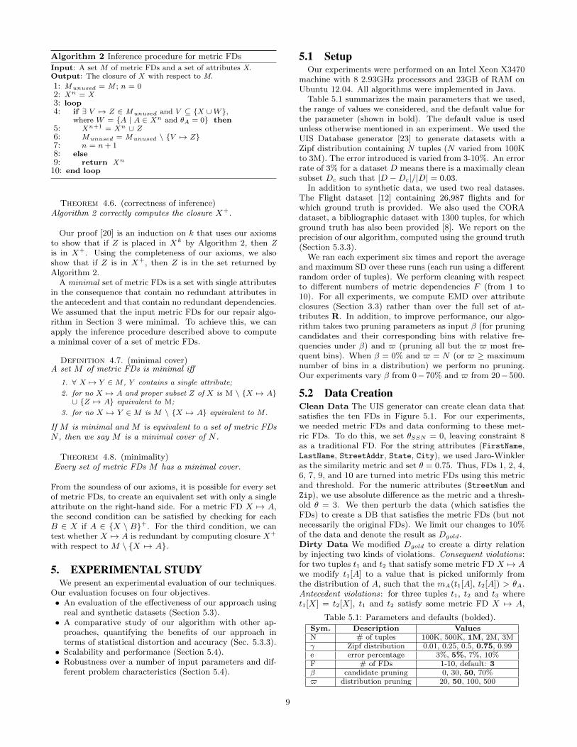
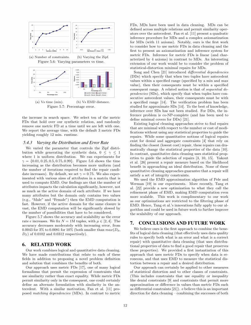
the increase in search space. We select ten of the metricFDs that hold over our synthetic relation, and randomlyremove one metric FD at a time until we are left with one.We report the average time, with the default 3 metric FDsyielding roughly 12 min. runtime.
5.4.3 Varying the Distribution and Error RateWe varied the parameter that controls the Zipf distri-
bution while generating the synthetic data, 0 ≤ γ ≤ 1where 1 is uniform distribution. We ran experiments forγ = {0.01, 0.25, 0.5, 0.75, 0.99}. Figure 5.6 shows the timeincreasing as the distribution becomes more uniform (andthe number of iterations required to find the repair candi-date increases). By default, we set γ = 0.75. We also exper-imented with various sizes of attributes in a matrix that isused to compute EMD. Our findings are that the number ofattributes impacts the calculation significantly, however, notas much as the active domain of each attribute. If we havemany attributes but the domain only contains two values(e.g., “Male” and “Female”) then the EMD computation isfast. However, if the active domain for the same closure isvast, the EMD computation will be significantly slowed bythe number of possibilities that have to be considered.
Figure 5.7 shows the accuracy and scalability as the errorrate e increases. We fix N = 1M tuples, with µ ∈ [2, 4]. Theaccuracy decreases moderately with increasing error, from0.0043 for 3% to 0.0081 for 10% (both smaller than max(Dd,DI) of 0.0102 and 0.0312 respectively).
6. RELATED WORKOur work combines logical and quantitative data cleaning.
We have made contributions that relate to each of thesefields in addition to proposing a novel problem definitionand solution that combines the benefits of both.
Our approach uses metric FDs [17], one of many logicalformalisms that permit the expression of constraints thatuse similarity rather than exact equality. While metric FDspermit similarity only in the consequent, one could certainlydefine an alternate formulation with similarity in the an-tecedent. With a similar motivation, Fan et al. [11] pro-posed matching dependencies (MDs). In contrast to metric
FDs, MDs have been used in data cleaning. MDs can bedefined across multiple relations and permit similarity oper-ators over the antecedent. Fan et al. [11] present a quadraticinference procedure for MDs and a complex axiomatizationfor MDs (with 11 axioms). Notably, ours is the first workto consider how to use metric FDs in data cleaning and thefirst to present an axiomatization and inference system formetric FDs. Inference for metric FDs is linear (and char-acterized by 4 axioms) in contrast to MDs. An interestingextension of our work would be to consider the problem ofstatistical-distortion minimal repairs for MDs.
Song and Chen [21] introduced differential dependencies(DDs) which specify that when two tuples have antecedentvalues within a specified range (specified by a min and maxvalue), then their consequents must be within a specifiedconsequent range. A related notion is that of sequential de-pendencies (SDs), which specify that when tuples have con-secutive antecedent values, their consequents must be witha specified range [14]. The verification problem has beenstudied for approximate SDs [14]. To the best of knowledge,inference over SDs has not been studied. For DDs, the in-ference problem is co-NP-complete (and has been used todefine minimal covers for DDs) [21].
Existing logical cleaning approaches strive to find repairsthat are minimal with respect to the number or cost of modi-fications without using any statistical properties to guide therepairs. While some quantitative notions of logical repairsexist for denial and aggregate constraints [4] that rely onfinding the closest (lowest cost) repair, these repairs can dra-matically change the statistical properties of the data [10].In contrast, quantitative data cleaning uses statistical prop-erties to guide the selection of repairs [3, 10, 15]. Yakoutet al. [26] present a repair measure based on the likelihoodbenefit in approaching an ideal distribution. None of thesequantitative cleaning approaches guarantee that a repair willsatisfy a set of integrity constraints.
We used the EMD approximation algorithm of Pele andWerman [19] in our experiments. More recently, Tang etal. [22] provide a new optimization to what they call therefinement phase of EMD, making EMD computation evenmore scalable. This work is complimentary to our workas our optimizations are restricted to the filtering phase ofEMD. Hence, Tang et al.’s innovations fully apply to our al-gorithm and could be used in future work to further improvethe scalability of our approach.
7. CONCLUSIONS AND FUTURE WORKWe believe ours is the first approach to combine the bene-
fits of logical data cleaning (that effectively uses data qualityrules to specify both what is an error and what is a correctrepair) with quantitative data cleaning (that uses distribu-tional properties of data to find a good repair that preservesthese properties). We provided a first instantiation of thisapproach that uses metric FDs to specify when data is er-roneous, and that uses EMD to measure the statistical dis-tortion between a repair and a desired distribution.
Our approach can certainly be applied to other measuresof statistical distortion and to other classes of constraints.(This includes constraints that use equality or inequalitylike denial constraints [9] and constraints that permit moreapproximation or difference in values than metric FDs suchas differential constraints [21]). e believe this is an importantdirection for data cleaning – combining the successes of both
12

logical and statistical approaches to provide more robustcleaning solutions.
8. REFERENCES[1] M. Arenas, L. E. Bertossi, and J. Chomicki. Consistent
query answers in inconsistent databases. In PODS, pages68–79, 1999.
[2] W. W. Armstrong. Dependency structures of data baserelationships. In IFIP Congress, pages 580–583, 1974.
[3] L. Berti-Equille, T. Dasu, and D. Srivastava. Discovery ofcomplex glitch patterns: A novel approach to quantitativedata cleaning. In ICDE, pages 733–744, 2011.
[4] L. Bertossi, L. Bravo, E. Franconi, and A. Lopatenko. Thecomplexity and approximation of fixing numericalattributes in databases under integrity constraints.Information Systems, 33(4–5):407–434, 2008.
[5] G. Beskales, I. F. Ilyas, and L. Golab. Sampling the repairsof functional dependency violations under hard constraints.PVLDB, 3(1):197–207, 2010.
[6] P. Bohannon, W. Fan, F. Geerts, X. Jia, andA. Kementsietsidis. Conditional functional dependencies fordata cleaning. In ICDE, pages 746–755, April 2007.
[7] P. Bohannon, M. Flaster, W. Fan, and R. Rastogi. Acost-based model and effective heuristic for repairingconstraints by value modification. In SIGMOD, pages143–154, 2005.
[8] F. Chiang and R. J. Miller. A unified model for data andconstraint repair. In ICDE, pages 446–457, 2011.
[9] X. Chu, F. Ilyas, and P. Papotti. Discovering DenialConstraints. PVLDB, 6(13):1498–1509, 2013.
[10] T. Dasu and J. M. Loh. Statistical distortion: Consequencesof data cleaning. PVLDB, 5(11):1674–1683, 2012.
[11] W. Fan, X. Jia, J. Li, and S. Ma. Reasoning about recordmatching rules. PVLDB, 2(1):407–418, 2009.
[12] Flights data.http://www.lunadong.com/fusionDataSets.htm.
[13] H. Galhardas, D. Florescu, D. Shasha, E. Simon, andC. Saita. Declarative data cleaning: Language, model, andalgorithms. In VLDB, pages 371–380, 2001.
[14] L. Golab, H. Karloff, F.Korn, A. Saha, and D. Srivastava.Sequential dependencies. PVLDB, 2(1):574–585, 2009.
[15] J. Hellerstein. Quantitative data cleaning for largedatabases. In Technical report, UC Berkeley, Feb 2008.
[16] S. Kolahi and L. Lakshmanan. On approximating optimumrepairs for functional dependency violations. In ICDT,pages 53–62, 2009.
[17] N. Koudas, A. Saha, D. Srivastava, andS. Venkatasubramanian. Metric Functional Dependencies.In ICDE, pages 1291–1294, 2009.
[18] O. Pele and M. Werman. A linear time histogram metricfor improved SIFT matching. In Eur. Conf. on ComputerVision, pages 495–508, 2008.
[19] O. Pele and M. Werman. Fast and robust earth mover’sdistances. In IEEE Int. Conf. on Computer Vision, pages460–467, 2009.
[20] N. Prokoshyna, J. Szlichta, F. Chiang, R. J. Miller, andD. Srivastava. Combining quantitative and logical datacleaning. April 2015.http://dblab.cs.toronto.edu/project/DataQuality.
[21] S. Song and L. Chen. Differential dependencies: Reasoningand discovery. TODS, 36(3):16, 2011.
[22] Y. Tang, L. H. U, Y. Cai, N. Mamoulis, and R. Cheng.Earth mover’s distance based similarity search at scale.Proc. VLDB Endow., 7(4):313–324, Dec. 2013.
[23] UIS Data Generator.http://www.cs.utexas.edu/users/ml/riddle/data.html.
[24] M. Volkovs, F. Chiang, J. Szchilta, and R. J. Miller.Continuous data cleaning. In ICDE, pages 244–255, 2014.
[25] X. Wang, X. L. Dong, and A. Meliou. Data x-ray: Adiagnostic tool for data errors. In SIGMOD, pages1231–1245, 2015.
[26] M. Yakout, L. Berti-Equille, and A. K. Elmagarmid. Don’tbe SCAREd: use SCalable Automatic REpairing withmaximal likelihood and bounded changes. In SIGMOD,pages 553–564, 2013.
[27] M. Zhang, M. Hadjieleftheriou, B. C. Ooi, C. M. Procopiuc,and D. Srivastava. On multi-column foreign key discovery.PVLDB, 3(1):805–814, 2010.
13

APPENDIXA. REASONING OVER METRIC FDS
We now provide proofs for our results on reasoning over metricFDs.
A.1 Metric FD AxiomatizationBelow we present the proof that our axioms (Identity, Decom-
position, Composition, and Limited Reduce) are sound and com-plete (Theorem 4.2).
Proof. First we prove that axioms are sound. That is, if M `X 7→ Y , then M |= X 7→ Y . The Identity axiom is clearly sound.We cannot have a relation D with two tuples that agree on X yetare not similar on X. To prove Decomposition, suppose we havea relation D that satisfies X 7→ YW . Let s, t ∈ D, such thats[X] = t[X]. This implies s[YW ] ≈mY W ,ΘY W
t[YW ], hence,s[Y ] ≈mY ,ΘY
t[Y ]. Therefore, D |= X 7→ Y . The soundnessof Composition is an extension of the argument given previously.Suppose we have a relation D that satisfies X 7→ Y and Z 7→W . Let s, t ∈ D, such that s[X] = t[X] and s[Z] = t[Z], thatis s[XZ] = t[XZ]. Since X 7→ Y and Z 7→ W , s[Y ] ≈mY ,ΘY
t[Y ] and s[W ] ≈mW ,ΘWt[W ] hold. This implies that s[YW ]
≈mY W ,ΘY Wt[YW ]. Therefore, D |= XZ 7→ YW . To prove
Limited Reduce, suppose we have a relation D that satisfies XY7→ Z, X 7→ Y and ΘY = 0. Let s, t ∈ D, such that s[X] = t[X].Therefore, since ΘY = 0 and X 7→ Y , this implies that s[XY ] =t[XY ]. As XY 7→ Y , it can be concluded that s[Z] ≈mZ ,ΘZ
t[Z].Therefore, D |= X 7→ Z.
Below we present the completeness proof (if M |= X 7→ Y ,then M ` X 7→ Y ). We consider a relation D with two rows asshown in Table A.1. We divide the attributes of a relation D intofour subsets: X; the set W , consisting of attributes in closureX+ minus attributes in X, for which distance threshold is set tozero; attributes in closure X+ minus attributes in W ∪X; and allremaining attributes. All the attributes in the relation D for thefirst row have the value a, while for the second row, the attributesin X are a’s, the attributes in W are a’s, the attributes in closureX+ minus attributes in W ∪ X are b’s and the other attributesare c’s. (For traditional FDs, by Transitivity if X functionallydetermines Y and Y functionally determines Z, then Z is in clo-sure X+; however, this is not necessarily true for metric FDs asshown in Example 4.1.) Without loss of generality, assume thatfor all attributes A over relation D we use the same metric m, a≈m,θA b, however, a 6= b. Furthermore, values a and c are notsimilar (a 6≈m,θA c).
We first show that D satisfies the set of metric FDs M (D|= M). Since metric FDs axioms are sound, metric FDs inferredfrom M are true. Assume V 7→ Z is in M but is not satisfied by arelation D. Therefore, V ⊆ {X ∪W} because otherwise two rowsof D are not equal on some attribute of V since for all attributesA over a relation D a ≈m,θA b, however, a 6= b and a 6≈m,θAc, and consequently a metric FD V 7→ Z would not be violated.Moreover, Z cannot be a subset of X+ (Z 6⊆ X+), or else V 7→Z would be satisfied by a relation D. Let A be an attribute of Znot in X+. Since, V ⊆ {X ∪W} ⊆ X+ by Lemma 4.4, X 7→ V .Also dependency V 7→ Z is in M , so by Decomposition, V 7→ A.By Composition XV 7→ V A can be inferred, therefore, XV 7→ Aby Decomposition. Let V = V1V2, where V1 ⊆ X and V2 ⊆ W .By Lemma 4.4, X 7→ V2 holds. As XV2 7→ A, X 7→ V2 and ΘV2= 0, by the Limited Reduce axiom X 7→ A. This would mean bythe definition of the closure that A is in X+, which we assumednot to be the case. Contradiction. A metric FD V 7→ Z which isin set of dependencies M is satisfied by relation D.
Our remaining proof obligation is to show that any metric FDnot inferable from the set of metric FDs M with metric FDsaxioms (M 6` X 7→ Y ) is not true (M 6|= X 7→ Y ). Suppose it issatisfied (M |= X 7→ Y ). By Reflexivity X 7→ X, so by Lemma4.4, X ⊆ X+. Since X ⊆ X+ it follows by the construction of arelation D that Y ⊆ X+. Otherwise, two rows of a relation D areequal on X but are not similar on some attribute A from Y . Then,from Lemma 4.4, it can be inferred that X 7→ Y . Contradiction.Therefore, whenever X 7→ Y does not follow from M by metricFDs axioms, M does not logically imply X 7→ Y . That is, theaxiom system is complete over metric FDs, which ends the proof.
Our proof of Lemma 4.4 makes use of an additional axiom, theUnion axiom, which follows directly from the Composition axiom.
Table A.1: Table template for metric FDs.
X+
X W = {A| A ∈ X+ \X X+ \ {X ∪W} Otherand θA = 0} attributes
a...a a...a a...a a...aa...a a...a b...b c...c
A.2 Closures (Lemma 4.4)Theorem A.1. (Union)
If X 7→ Y and X 7→ Z, then X 7→ Y Z.
Proof. We are given metric FDs X 7→ Y and X 7→ Z, there-fore we can use the Composition axiom to infer XX 7→ Y Z.Hence, X 7→ Y Z holds.
We now prove Lemma 4.4 stating that M ` X 7→ Y iff Y ⊆X+.
Proof. Let Y = {A1, ..., An}. Assume Y ⊆ X+. By defi-nition of X+, X 7→ Ai, for all i ∈ {1, ..., n}. Therefore, by theUnion inference rule, X 7→ Y follows.
For the other direction, suppose X 7→ Y follows from the ax-ioms. For each i ∈ {1, ..., n}, X 7→ Ai by the Decompositionaxiom, hence Y ⊆ X+.
A.3 Proof of Theorem 4.6Algorithm 2 correctly computes closure X+.
Proof. First we show by induction on k that if Z is placed inX k by Algorithm 2, then Z is in X+.Basis: k = 0. By Identity axiom X 7→ X.Induction: k > 0. Assume that X k−1 consists only of attributesin X+. Suppose Z is placed in X k because V 7→ Z, and V ⊆X∪W . Let V = V1V2, where V1 ⊆X and V2 ⊆W . By ReflexivityX 7→ V1. Since V2 ⊆ W by Lemma 4.4, X 7→ V2. Therefore, bythe Union inference rule X 7→ V . Hence, by Composition XV 7→V Z holds. Thus, by Limited Reduce X 7→ V Z as ΘV2
= 0, andby Decomposition X 7→ Z is true.
Now we prove the opposite, if Z is in X+, then Z is in the setreturned by Algorithm 2. Suppose Z is in X+ but Z is not inthe set returned by Algorithm 2. Consider a relation D similar tothe one shown in Table A.1. A relation D has two tuples that areequal on attributes in X ∪ W , are similar but not equal on Xn
\ {X ∪W} and are not similar on all other attributes. We claimthat D satisfies M . If not, let P 7→ O be a dependency in M thatis violated by D. Then P ⊆ X∪W and set of attributes O cannotbe a subset of Xn, if the violation happens. (Similar argumentwas used in the proof of Theorem 4.2.) Thus, by Algorithm 2,Lines 4–7 there exists Xn+1, which is a contradiction.
A.4 Proof of Theorem 4.8Every set of metric FDs M has a minimal cover.
Proof. By the Union and Decomposition inference rules, it ispossible to have M with only a single attribute in the right handside. Second (no redundant attributes) and third (no redundantdependencies) conditions can be satisfied by repeatedly deletingan attribute and then repeatedly removing a dependency. We cantest whether an attribute B from X is redundant for the metricFD X 7→ A by checking if A is in {X \B}+. We can test whetherX 7→ A is redundant by computing closure X+ with respect toM \ {X 7→ A}.
B. SD MINIMAL REPAIRSB.1 Proof of Theorem 2.11
The problem of finding a statistical-distortion minimal repairis NP-hard.
Proof. Let F be a set of FDs over R where |R| = d. Let Ibe an instance of R. Let R′ be R with d+ 1 additional columns~Id = Id1, ..., Idd+1. Let I′ be I where each Idi contains a unique
14

value for each tuple of I (i.e., each Idi is a key for I′). If Dr isa cardinality-minimal repair for I′ and F over R′ then ΠR(Dr)is a cardinality-minimal repair for I = ΠR(I′) and F over R.Similarly, suppose Dr is a cardinality-minimal repair for I and F .
Let I′ contain unique values on all attributes in ~Id and ΠR(I′) =I. Then Dr extended to Dr’ such that Π ~Id
(I′) = ΠvecId(Dr ′) is
a cardinality-minimal repair for F over R′ and I′.
Let Mi be a key dependency (FD) on R′ : Idi → R ∪ ~Id.Without loss of generality, we assume F is a minimal cover, soeach f ∈ F has the form X 7→ A. Let M be a set of metric FDs(on R′) constructed as follows from F . First, Mi ∈ M for all1 ≤ i ≤ d + 1. In addition, for each (X 7→ A) ∈ F , let (X 7→ A)with metric mA and threshold ΘA = 0 be in M. We definemA(a1, a2) = 0 if a1 = a2, and 1 otherwise.
Let Dr be a repair for I′ (therefore ΠR(Dr) is a repair for I).Let DI = I′. We claim that Dr is a cardinality-minimal repairfor F iff Dr is a statistical-distortion minimal repair for M.
(⇒) Let Dr be a cardinality-minimal repair of F for I′. LetV be the set of changes used to create Dr from I′. Then clearlyDr is a set-minimal repair of M. This follows from the factthat every cardinality-minimal repair is set minimal and also fromthe construction of M. If Dr |= F , then necessarily Dr |= M.We need to show that Dr is statistical-distortion minimal repairmeaning that EMD(Dr, DI) is minimal.
The distributions of both Dr and DI each contain n bins, eachcorresponding to a single tuple (so n = |I′|) and each bin hasweight 1. Let t ∈ I′. We need to flow or change t into one of thetuples t′ from Dr. The lowest cost way to do this is to changeeach t into a t′ where Π ~Id
(t) = Π ~Id(t′). Such a change would have
a cost of d or less, where as changing t to any other tuple in Drwould have a cost of at least d+ 1. Hence, the EMD cost is 1 foreach value of an attribute in R that has been changed in Dr fromthe original I′ = DI . Therefore, EMD(Dr, DI) = |V| (where Vis the set of changes used to create Dr from I′ = DI). If there is arepair with a lower statistical distortion from DI , then Dr is nota cardinality-minimal repair. Hence, Dr is a statistical-distortionminimal repair for M.
(⇐) Let Dr be a statistical-distortion minimal repair for Mover R′. Let V be the set of changes used to create Dr from I′.We need to show that Dr is cardinality-minimal.
As in the first half of the proof, the EMD cost is 1 for eachvalue of an attribute in R that has been changed in Dr fromthe original I′ = DI . Also EMD(Dr, DI) = |V|. If there is avalue of an attribute that could be reverted to the original valuewithout Dr 6|= M, then there is a repair where EMD cost forthat value of an attribute is 0, and Dr would not be statistically-distortion minimal, which is a contradiction. Therefore, |V| hasthe smallest possible number of changes for all repairs. Thus, Dris a cardinality-minimal repair for M.
B.2 Proof of Theorem 3.3The relation Dr that is generated by Algorithm 1 is a set-
minimal repair of the input inconsistent relation Dd over the setof metric FDs M .
Proof. We need to prove the following: a) generated relationDr is a repair (Definition 2.5) of inconsistent relation Dd overthe set of metric FDs M ; b) generated repair Dr is set-minimal(Definition 2.6).
To prove that relation Dr is a repair of relation Dd, we showthat Dr is consistent and tuples in Dd are carried over to Dr.We prove this by induction over tuples. We show in the induc-tion step that if relation Dc is consistent, then Dc = {Dc ∪ tr} isconsistent, where a tuple tr is modified from a tuple td ∈ Du (andDu denotes unresolved tuples) by consequent repairs (Algorithm1 Line 9), antecedent repairs (Algorithm 1 Line 18) or otherwiseboth consequent and antecedent repairs (Algorithm 1 Line 26).That is {Dc ∪ tr} is consistent since repairs to attributes in boththe antecedents and consequents always guarantee resolving in-consistencies, as they are conducted with respect to clean tuplet ∈ Dc, i.e., tr[Z] = t[Z], where Z represents closure of all at-tributes in violated dependencies. After this step, we choose amaximal subset of reverts of attribute values of tuple tr w.r.t. td,denoted as t′r, such that {Dc ∪ t′r} |= M (Algorithm 1 Line 34).Therefore, upon termination of the algorithm, relation Dr = Dc
(Algorithm 1 Line 35) contains all modified tuples from Dd andis consistent by the induction step.
To prove that generated repair Dr is set-minimal, we needto show that any subset of changed attribute values cannot bereverted to their original values in relation Dd without violatingthe set of prescribed metric FDs M . Let t0, t1, .., tn be the orderin which tuples are inserted into Dc in Algorithm 1. We prove byinduction that every attribute value from tuples t0,..., ti, where0 ≤ i ≤ n, is either an unchanged attribute value or a changedattribute value that represents a necessary change.
1. Base Case: initial dataset Dc = {t0, ..., tm} (where m < n)is a maximal consistent set of tuples from relation Dd, andtherefore, t0, ..., tm remains unchanged.
2. Induction Step: we show that if every attribute value fromtuples t0, .., ti is either unchanged or necessarily changed,attribute values in ti+1 are either unchanged or necessar-ily changed. If attribute values in ti+1 are unchanged, theinduction step is correct. Otherwise, ti+1 is changed andwe have to show that changing values in ti+1 was neces-sary. We prove this by contradiction. Assume we can revertattribute values C of tuple ti+1 to their original values inDd without violating the set of metric FDs M . However,in this case, Algorithm 1 would not change C, as it tries torevert all possible subsets of attribute values in the tuple trback to their original values in td to obtain a tuple t′r, suchthat Dc ∪ t′r |= M and choose the maximal subset satisfyingthis condition, denoted as min(tr) (Algorithm 1 Line 34).Therefore, we reach contradiction.
Hence, it follows that every attribute value change in datasetDr = Dc = {t0, ..., tn} is a necessary change, which implies thatDr is set-minimal.
15