combining principal component analysis, discrete wavelet ...€¦ · combining principal component...
TRANSCRIPT

Combining Principal Component Analysis, Discrete WaveletTransform and XGBoost to trade in the Financial Markets
João Pedro Pinto Brito Nobre
Thesis to obtain the Master of Science Degree in
Electrical and Computer Engineering
Supervisor: Prof. Rui Fuentecilla Maia Ferreira Neves
Examination Committee
Chairperson: Prof. António Manuel Raminhos Cordeiro GriloSupervisor: Prof. Rui Fuentecilla Maia Ferreira Neves
Member of the Committee: Prof. Aleksandar Ilic
June 2018

ii

Declaration
I declare that this document is an original work of my own authorship and that it fulfills all the require-
ments of the Code of Conduct and Good Practices of the Universidade de Lisboa.
iii

iv

”The stock market is filled with individuals who know the price of everything, but the value of nothing.”
Phillip Fisher
v

vi

Acknowledgments
I would first like to thank my supervisor, Prof. Rui Neves, for all the support and feedback given in the
course of this thesis. His guidance and feedback given were helpful to always be on the right track and
contributed a lot to increase my knowledge on the subject.
I would also like to thank my friends and colleagues with whom I shared many joyful moments during
my academic path.
To my family, who always supported me in my academic path and personal life, I am eternally grateful.
Their constant encouragement throughout writing this thesis allowed me to overcome every obstacle that
arose.
vii

viii
Resumo
Esta tese apresenta uma abordagem que combina a Analise de Componentes Principais (PCA), a
Transformada Wavelet Discreta (DWT), Extreme Gradient Boosting (XGBoost) e um Algoritmo Genetico
para Multi-Optimizacao (MOO-GA) para criar um sistema capaz de obter retornos elevados com um
baixo nıvel de risco associado as transacoes.
A PCA e utilizada para reduzir a dimensionalidade do conjunto de dados financeiros mantendo
sempre as partes mais importantes de cada feature e a DWT e utlizada para efectuar uma reducao
de ruıdo a cada feature mantendo sempre a sua estrutura. O conjunto de dados resultante e entao
entregue ao classificador binario XGBoost que tem os seus hiper-parametros optimizados recorrendo a
um MOO-GA de forma a obter, para cada mercado financeiro analisado, o melhor desempenho.
A abordagem proposta e testada com dados financeiros reais provenientes de cinco mercados fi-
nanceiros diferentes, cada um com as suas caracterısticas e comportamento. A importancia do PCA
e da DWT e analisada e os resultados obtidos demonstram que, quando aplicados separadamente, o
desempenho dos dois sistemas e melhorado. Dada esta capacidade em melhorar os resultados obti-
dos, o PCA e a DWT sao entao aplicados conjuntamente num unico sistema e os resultados obtidos
demonstram que este sistema e capaz de superar a estrategia de Buy and Hold (B&H) em quatro dos
cinco mercados financeiros analisados, obtendo uma taxa de retorno media de 49.26% no portfolio,
enquanto o B&H obtem, em media, 32.41%.
Palavras-chave: Mercados Financeiros, Analise de Componentes Principais (PCA), Trans-
formada Wavelet Discreta (DWT), Extreme Gradient Boosting (XGBoost), Algoritmo Genetico para Multi-
Optimizacao (MOO-GA), Reducao de Dimensao, Reducao de Ruıdo.
ix

x

Abstract
This thesis presents an approach combining Principal Component Analysis (PCA), Discrete Wavelet
Transform (DWT), Extreme Gradient Boosting (XGBoost) and a Multi-Objective Optimization Genetic
Algorithm (MOO-GA) to create a system that is capable of achieving high returns with a low level of risk
associated to the trades.
PCA is used to reduce the dimensionality of the financial input data set while maintaining the most
valuable parts of each feature and the DWT is used to perform a noise reduction to every feature while
keeping its structure. The resultant data set is then fed to an XGBoost binary classifier that has its
hyperparameters optimized by a MOO-GA in order to achieve, for every analyzed financial market, the
best performance.
The proposed approach is tested with real financial data from five different financial markets, each
with its own characteristics and behavior. The importance of the PCA and the DWT is analyzed and
the results obtained show that, when applied separately, the performance of both systems is improved.
Given their ability in improving the results obtained, the PCA and the DWT are then applied together
in one system and the results obtained show that this system is capable of outperforming the Buy and
Hold (B&H) strategy in four of the five analyzed financial markets, achieving an average rate of return of
49.26% in the portfolio, while the B&H achieves on average 32.41%.
Keywords: Financial Markets, Principal Component Analysis (PCA), Discrete Wavelet Trans-
form (DWT), Extreme Gradient Boosting (XGBoost), Multi-Objective Optimization Genetic Algorithm
(MOO-GA), Dimensionality Reduction, Noise Reduction.
xi

xii

Contents
Declaration . . . . . . . . . . . . . . . . . . . . . . . . . . . . . . . . . . . . . . . . . . . . . . . iii
Acknowledgments . . . . . . . . . . . . . . . . . . . . . . . . . . . . . . . . . . . . . . . . . . . vii
Resumo . . . . . . . . . . . . . . . . . . . . . . . . . . . . . . . . . . . . . . . . . . . . . . . . . ix
Abstract . . . . . . . . . . . . . . . . . . . . . . . . . . . . . . . . . . . . . . . . . . . . . . . . . xi
List of Tables . . . . . . . . . . . . . . . . . . . . . . . . . . . . . . . . . . . . . . . . . . . . . . xv
List of Figures . . . . . . . . . . . . . . . . . . . . . . . . . . . . . . . . . . . . . . . . . . . . . xvii
List of Acronyms . . . . . . . . . . . . . . . . . . . . . . . . . . . . . . . . . . . . . . . . . . . . xxi
Glossary . . . . . . . . . . . . . . . . . . . . . . . . . . . . . . . . . . . . . . . . . . . . . . . . 1
1 Introduction 1
1.1 Motivation . . . . . . . . . . . . . . . . . . . . . . . . . . . . . . . . . . . . . . . . . . . . . 2
1.2 Work’s purpose . . . . . . . . . . . . . . . . . . . . . . . . . . . . . . . . . . . . . . . . . . 3
1.3 Main Contributions . . . . . . . . . . . . . . . . . . . . . . . . . . . . . . . . . . . . . . . . 3
1.4 Thesis Outline . . . . . . . . . . . . . . . . . . . . . . . . . . . . . . . . . . . . . . . . . . 3
2 Related Work 4
2.1 Market Analysis . . . . . . . . . . . . . . . . . . . . . . . . . . . . . . . . . . . . . . . . . . 4
2.1.1 Fundamental Analysis . . . . . . . . . . . . . . . . . . . . . . . . . . . . . . . . . . 5
2.1.2 Technical Analysis . . . . . . . . . . . . . . . . . . . . . . . . . . . . . . . . . . . . 5
2.1.3 Machine Learning . . . . . . . . . . . . . . . . . . . . . . . . . . . . . . . . . . . . 16
2.2 Principal Component Analysis . . . . . . . . . . . . . . . . . . . . . . . . . . . . . . . . . . 16
2.3 Wavelet Transform . . . . . . . . . . . . . . . . . . . . . . . . . . . . . . . . . . . . . . . . 20
2.3.1 Continuous Wavelet Transform . . . . . . . . . . . . . . . . . . . . . . . . . . . . . 22
2.3.2 Discrete Wavelet Transform . . . . . . . . . . . . . . . . . . . . . . . . . . . . . . . 22
2.4 Extreme Gradient Boosting . . . . . . . . . . . . . . . . . . . . . . . . . . . . . . . . . . . 27
2.5 Genetic Algorithm . . . . . . . . . . . . . . . . . . . . . . . . . . . . . . . . . . . . . . . . 30
2.5.1 Multi-Objective Optimization . . . . . . . . . . . . . . . . . . . . . . . . . . . . . . . 31
2.6 Relevant studies . . . . . . . . . . . . . . . . . . . . . . . . . . . . . . . . . . . . . . . . . 34
3 Implementation 36
3.1 System’s Architecture . . . . . . . . . . . . . . . . . . . . . . . . . . . . . . . . . . . . . . 36
3.2 Target Formulation . . . . . . . . . . . . . . . . . . . . . . . . . . . . . . . . . . . . . . . . 37
xiii
3.3 Financial Data Module . . . . . . . . . . . . . . . . . . . . . . . . . . . . . . . . . . . . . . 38
3.4 Technical Analysis Module . . . . . . . . . . . . . . . . . . . . . . . . . . . . . . . . . . . . 38
3.5 Data Preprocessing Module . . . . . . . . . . . . . . . . . . . . . . . . . . . . . . . . . . . 39
3.5.1 Data Normalization Module . . . . . . . . . . . . . . . . . . . . . . . . . . . . . . . 41
3.5.2 PCA Module . . . . . . . . . . . . . . . . . . . . . . . . . . . . . . . . . . . . . . . 42
3.5.3 Wavelet Module . . . . . . . . . . . . . . . . . . . . . . . . . . . . . . . . . . . . . 43
3.6 XGBoost Module . . . . . . . . . . . . . . . . . . . . . . . . . . . . . . . . . . . . . . . . . 46
3.6.1 XGBoost Binary Classifier Module . . . . . . . . . . . . . . . . . . . . . . . . . . . 46
3.6.2 Multi-Objective Optimization GA Module . . . . . . . . . . . . . . . . . . . . . . . . 50
3.7 Trading Module . . . . . . . . . . . . . . . . . . . . . . . . . . . . . . . . . . . . . . . . . . 57
4 Results 60
4.1 Financial Data . . . . . . . . . . . . . . . . . . . . . . . . . . . . . . . . . . . . . . . . . . 61
4.2 Evaluation metrics . . . . . . . . . . . . . . . . . . . . . . . . . . . . . . . . . . . . . . . . 61
4.3 System Parameters . . . . . . . . . . . . . . . . . . . . . . . . . . . . . . . . . . . . . . . 63
4.4 Case Study I - Influence of the PCA technique . . . . . . . . . . . . . . . . . . . . . . . . 63
4.5 Case Study II - Influence of the DWT denoise . . . . . . . . . . . . . . . . . . . . . . . . . 66
4.6 Case Study III - Combining PCA and DWT . . . . . . . . . . . . . . . . . . . . . . . . . . . 70
4.7 Case Study IV - Performance Comparison . . . . . . . . . . . . . . . . . . . . . . . . . . . 77
5 Conclusions 79
5.1 Conclusions . . . . . . . . . . . . . . . . . . . . . . . . . . . . . . . . . . . . . . . . . . . . 79
5.2 Future Work . . . . . . . . . . . . . . . . . . . . . . . . . . . . . . . . . . . . . . . . . . . . 80
Bibliography 81
A Return Plots of the Case Study I 86
A.1 Brent Crude futures contract . . . . . . . . . . . . . . . . . . . . . . . . . . . . . . . . . . 86
A.2 Corn futures contract . . . . . . . . . . . . . . . . . . . . . . . . . . . . . . . . . . . . . . . 87
A.3 Exxon Mobil Corporation stocks . . . . . . . . . . . . . . . . . . . . . . . . . . . . . . . . . 88
A.4 Home Depot Inc. stocks . . . . . . . . . . . . . . . . . . . . . . . . . . . . . . . . . . . . . 89
A.5 S&P 500 index . . . . . . . . . . . . . . . . . . . . . . . . . . . . . . . . . . . . . . . . . . 90
B Return Plots of the Case Study II 91
B.1 Brent Crude futures contract . . . . . . . . . . . . . . . . . . . . . . . . . . . . . . . . . . 91
B.2 Corn futures contract . . . . . . . . . . . . . . . . . . . . . . . . . . . . . . . . . . . . . . . 92
B.3 Exxon Mobil Corporation stocks . . . . . . . . . . . . . . . . . . . . . . . . . . . . . . . . . 93
B.4 Home Depot Inc. stocks . . . . . . . . . . . . . . . . . . . . . . . . . . . . . . . . . . . . . 94
B.5 S&P 500 index . . . . . . . . . . . . . . . . . . . . . . . . . . . . . . . . . . . . . . . . . . 95
xiv
List of Tables
2.1 Summary of the most relevant studies related with this thesis. . . . . . . . . . . . . . . . . 35
3.1 List of the 31 features output to the data preprocessing module. . . . . . . . . . . . . . . . 40
3.2 Principal components of the 31 features from the daily S&P 500 index data (from 02/10/2006
to 11/01/2018). . . . . . . . . . . . . . . . . . . . . . . . . . . . . . . . . . . . . . . . . . . 44
4.1 Fixed parameters of the implemented system. . . . . . . . . . . . . . . . . . . . . . . . . . 63
4.2 B&H results and average results of the basic system and the system with PCA. . . . . . . 64
4.3 B&H results and average results of the basic system and the system with DWT. . . . . . . 68
4.4 B&H results and average results of the system with PCA, with DWT and with PCA and DWT. 72
4.5 B&H results and average results of the proposed system and the system proposed by
Nadkarni. . . . . . . . . . . . . . . . . . . . . . . . . . . . . . . . . . . . . . . . . . . . . . 78
xv

xvi

List of Figures
2.1 S&P 500 index close prices and respective 10-day SMA and 10-day EMA plot. . . . . . . 7
2.2 S&P 500 index close prices and respective Bollinger bands (lower, middle and upper) plot. 7
2.3 S&P 500 index close prices and respective RSI plot. . . . . . . . . . . . . . . . . . . . . . 9
2.4 S&P 500 index close prices and respective MACD plot. . . . . . . . . . . . . . . . . . . . 11
2.5 S&P 500 index close prices and respective OBV line plot. . . . . . . . . . . . . . . . . . . 14
2.6 Plot of the two principal components in the data set. . . . . . . . . . . . . . . . . . . . . . 18
2.7 Projection of the data onto the two principal components. . . . . . . . . . . . . . . . . . . 19
2.8 Examples of wavelet basis. (a) Haar. (b) Symlet of order 4. (c) Daubechies of order 3. (d)
Daubechies of order 4. . . . . . . . . . . . . . . . . . . . . . . . . . . . . . . . . . . . . . . 21
2.9 DWT decomposition of a signal for a decomposition level of 2. . . . . . . . . . . . . . . . . 23
2.10 DWT approximation and detail coefficients for a decomposition level of 3. . . . . . . . . . 24
2.11 DWT reconstruction of a signal for a decomposition level of 2. . . . . . . . . . . . . . . . . 24
2.12 Gradient Descent method. . . . . . . . . . . . . . . . . . . . . . . . . . . . . . . . . . . . . 28
2.13 Single-Point Crossover and Two-Point Crossover. . . . . . . . . . . . . . . . . . . . . . . . 31
2.14 Set of solutions with respective Pareto front. . . . . . . . . . . . . . . . . . . . . . . . . . . 32
2.15 Multi-objective optimization process. . . . . . . . . . . . . . . . . . . . . . . . . . . . . . . 33
3.1 Architecture of the proposed system. . . . . . . . . . . . . . . . . . . . . . . . . . . . . . . 36
3.2 S&P 500 index historical data format. . . . . . . . . . . . . . . . . . . . . . . . . . . . . . 39
3.3 Data preprocessing module. . . . . . . . . . . . . . . . . . . . . . . . . . . . . . . . . . . . 41
3.4 XGBoost binary classifier model. . . . . . . . . . . . . . . . . . . . . . . . . . . . . . . . . 46
3.5 Inputs to the XGBoost binary classifier. . . . . . . . . . . . . . . . . . . . . . . . . . . . . 47
3.6 XGBoost classifier architecture. . . . . . . . . . . . . . . . . . . . . . . . . . . . . . . . . . 48
3.7 Boosted tree plot. . . . . . . . . . . . . . . . . . . . . . . . . . . . . . . . . . . . . . . . . . 49
3.8 Feature importance plot. . . . . . . . . . . . . . . . . . . . . . . . . . . . . . . . . . . . . . 50
3.9 Hyperparameters optimization process. . . . . . . . . . . . . . . . . . . . . . . . . . . . . 50
3.10 Non-dominated sorting based upon ranking and crowding distance. . . . . . . . . . . . . 52
3.11 Calculation of the final fitness value. . . . . . . . . . . . . . . . . . . . . . . . . . . . . . . 56
3.12 State machine diagram of the trading module. . . . . . . . . . . . . . . . . . . . . . . . . . 58
3.13 Trading module execution example with S&P 500 data. . . . . . . . . . . . . . . . . . . . . 59
xvii
4.1 B&H returns and average returns of the basic system and the system with PCA, for the
Corn futures contract. . . . . . . . . . . . . . . . . . . . . . . . . . . . . . . . . . . . . . . 67
4.2 B&H returns and average returns of the basic system and the system with PCA, for the
Exxon Mobil Corporation stocks. . . . . . . . . . . . . . . . . . . . . . . . . . . . . . . . . 67
4.3 B&H returns and average returns of the basic system and the system with Haar wavelet
with a level of decomposition of 5, for the Corn futures contract. . . . . . . . . . . . . . . . 70
4.4 B&H returns and average returns of the basic system and the system with Haar wavelet
with a level of decomposition of 5, for the Exxon Mobil Corporation stocks. . . . . . . . . . 71
4.5 B&H returns and the best and average returns of the system with PCA and Haar wavelet
with a level of decomposition of 5, for the Brent Crude futures contract. . . . . . . . . . . . 74
4.6 B&H returns and the best and average returns of the system with PCA and Haar wavelet
with a level of decomposition of 5, for the Corn futures contract. . . . . . . . . . . . . . . . 75
4.7 B&H returns and the best and average returns of the system with PCA and Haar wavelet
with a level of decomposition of 5, for the Exxon Mobil Corporation stocks. . . . . . . . . . 75
4.8 B&H returns and the best and average returns of the system with PCA and Db3 wavelet
with a level of decomposition of 5, for the Home Depot Inc. stocks. . . . . . . . . . . . . . 76
4.9 B&H returns and the best and average returns of the system with PCA and Haar wavelet
with a level of decomposition of 5, for the S&P 500 Index. . . . . . . . . . . . . . . . . . . 76
4.10 B&H returns and average returns of the portfolio, using the system combining PCA and
DWT. . . . . . . . . . . . . . . . . . . . . . . . . . . . . . . . . . . . . . . . . . . . . . . . . 77
A.1 B&H returns and average returns of the basic system and the system with PCA, for the
Brent Crude futures contract. . . . . . . . . . . . . . . . . . . . . . . . . . . . . . . . . . . 86
A.2 B&H returns and average returns of the basic system and the system with PCA, for the
Corn futures contract. . . . . . . . . . . . . . . . . . . . . . . . . . . . . . . . . . . . . . . 87
A.3 B&H returns and average returns of the basic system and the system with PCA, for the
Exxon Mobil Corporation stocks. . . . . . . . . . . . . . . . . . . . . . . . . . . . . . . . . 88
A.4 B&H returns and average returns of the basic system and the system with PCA, for the
Home Depot Inc. stocks. . . . . . . . . . . . . . . . . . . . . . . . . . . . . . . . . . . . . . 89
A.5 B&H returns and average returns of the basic system and the system with PCA, for the
S&P 500 Index. . . . . . . . . . . . . . . . . . . . . . . . . . . . . . . . . . . . . . . . . . . 90
B.1 B&H returns and average returns of the basic system and the system with Haar wavelet
with a level of decomposition of 5, for the Brent Crude futures contract. . . . . . . . . . . . 91
B.2 B&H returns and average returns of the basic system and the system with Haar wavelet
with a level of decomposition of 5, for the Corn futures contract. . . . . . . . . . . . . . . . 92
B.3 B&H returns and average returns of the basic system and the system with Haar wavelet
with a level of decomposition of 5, for the Exxon Mobil Corporation stocks. . . . . . . . . . 93
B.4 B&H returns and average returns of the basic system and the system with Db3 wavelet
with a level of decomposition of 5, for the Home Depot Inc. stocks. . . . . . . . . . . . . . 94
xviii

B.5 B&H returns and average returns of the basic system and the system with Haar wavelet
with a level of decomposition of 5, for the S&P 500 Index. . . . . . . . . . . . . . . . . . . 95
xix

xx
List of Acronyms
ABC Artificial Bee Colony
ADX Average Directional Index
ANN Artificial Neural Network
ARIMA Autoregressive Integrated Moving Average
ATR Average True Range
AUC Area Under the Curve
B&H Buy and Hold
CCI Commodity Channel Index
CWT Continuous Wavelet Transform
DI Directional Indicator
DM Directional Movement
DWT Discrete Wavelet Transform
EMA Exponential Moving Average
EMH Efficient Market Hypothesis
FRPCA Fast Robust Principal Component Analysis
GA Genetic Algorithm
KPCA Kernel Principal Component Analysis
MDD Max Drawdown
MFI Money Flow Index
MACD Moving Average Convergence Divergence
MOEA Multi-Objective Evolutionary Algorithm
MOO-GA Multi-Objective Optimization Genetic Algorithm
xxi
MOO Multi-Objective Optimization
NEAT NeuroEvolution of Augmenting Topologies
NSGA-II Non-dominated Sorting Genetic Algorithm-II
OBV On Balance Volume
PCA Principal Component Analysis
PPO Percentage Price Oscillator
PSAR Parabolic Stop and Reversal
RNN Recurrent Neural Network
ROC Rate of Change
ROR Rate of Return
RRR Risk Return Ratio
RSI Relative Strength Index
SOO Single-Objective Optimization
SMA Simple Moving Average
SVM Support Vector Machine
TA Technical Analysis
TP Typical Price
TR True Range
VIX Volatility Index
XGBoost Extreme Gradient Boosting
xxii
Chapter 1
Introduction
The continuous evolution in the Machine Learning and Artificial Intelligence areas and the fact that the
financial markets information is becoming more accessible to a larger number of investors results in
the appearance of sophisticated trading algorithms that consequently are starting to have a significant
influence on the market’s behaviour.
The main objective of an investor is to develop a low-risk trading strategy that determines the best
time to buy or sell the stocks. Since financial markets are influenced by many factors such as political
or economic factors, this is a difficult task because financial market signals are noisy, non-linear and
non-stationary.
According to the Efficient Market Hypothesis (EMH) [1], a financial market time series is nearly
unforecastable and that is because it’s impossible to beat the market since the share prices already
have all the relevant available information into account, including the past prices and trading volumes.
As such, price fluctuations respond immediately to new information and don’t follow any pattern, being
unpredictable and stopping investors from earning above average returns without taking many risks.
The EMH states that no investor should ever be able to beat the market and that the best investment
strategy is the Buy and Hold (B&H) strategy where an investor simply buys the stocks and holds them
for as long as he wants, regardless of price fluctuations. This hypothesis consequently implies that a
binary classifier that tries to identify if the difference between the price of a stock in a day with the price
of the same stock in the day after is positive or negative wouldn’t perform better than random guessing
since the market price will always be the fair one, and therefore unpredictable.
In order to help a trader to analyze stocks and make investment decisions there are two main meth-
ods used to analyze the market movements: Technical and Fundamental analysis. Technical analysis
mainly focus on the financial market’s time series and tries to determine the trend of the price and search
for predictable patterns, while Fundamental analysis is more focused on determining if the current stock
price is reasonable, having into account the company’s performance and financial status. They both
have different utilities, with the Technical analysis being more useful in short-term trading and the Fun-
damental analysis in long-term trading. With the advances in the field of Machine Learning and Artificial
Intelligence, the exclusive use of Technical and Fundamental analysis to study the market’s behaviour is
1

being surpassed by the use of algorithms and models that incorporate many data mining and prediction
techniques used to forecast the direction of a stock’s price, achieving higher returns with lower risks.
In this thesis, an approach combining Principal Component Analysis (PCA) for dimensionality re-
duction, the Discrete Wavelet Transform (DWT) for noise reduction and an XGBoost (Extreme Gradient
Boosting) binary classifier whose hyperparameters are optimized using a Multi-Objective Optimization
Genetic Algorithm (MOO-GA), is presented. Using PCA the high dimensional financial input data set
is reduced to a lower dimensional one, maximizing the variance in the lower dimensional space and
while keeping the main essence of the original data set. This dimensionality reduction allows for a better
identification of patterns in the training data that consecutively results in a better generalization ability
and an higher accuracy by the XGBoost binary classifier. The DWT further performs noise reduction
to this reduced data set in order to remove irrelevant data samples that may have a negative impact
in the performance of the system, while still preserving the main structure of the data. The XGBoost
binary classifier has its hyperparameters optimized using the MOO-GA in order to achieve the best
performance for each analyzed financial market. Then, the classifier is trained using the set of hyperpa-
rameters obtained through the optimization process and, using the predictions made, it outputs a trading
signal with the buy and sell orders, with the objective of maximizing the returns, while minimizing the
levels of risk associated to the trades made.
1.1 Motivation
The main motivation when trying to develop a model to forecast the direction of the stock market is trying
to achieve financial gains. From an engineering point of view, applying signal processing and machine
learning methods to explore the non-linear and non-stationary characteristics of a signal, as well as its
noisy nature is also one of the main motivations for this work.
Another motivation for this work is the use of XGBoost to classify the market’s direction of the next
day. XGBoost has been applied to many classification and regression problems but its use in the stock
market is nearly nonexistent. By exploring the XGBoost classification capacities it is possible to obtain
a trading signal with entry and exit points and implement an automated trading strategy, which isn’t very
common in similar studies since most of them are mainly focused on forecasting the price of a stock and
the direction, but didn’t develop a trading strategy to make use of that forecasts.
Furthermore, one of the main motivations for this work is the use of the PCA together with the DWT
to improve the system’s performance and achieve higher returns, for which there are also few studies
applying it to financial market forecasting. By combining the PCA dimensionality reduction technique
with the DWT noise reduction, the objective is to verify if the XGBoost binary classifier performance is
improved by not only discovering the most important features in the financial data but also removing
irrelevant data samples, in order to achieve a higher accuracy and higher returns.
The optimization of the hyperparameters of the XGBoost binary classifier using a MOO-GA is also
an unexplored subject, since most studies only focus on optimizing one objective function in a given
problem. Thus, by combining these different machine learning methods, this thesis presents a novel
2

approach for the forecasting of financial markets that was never done before.
1.2 Work’s purpose
The aim of this thesis is to examine the applicability of PCA for dimensionality reduction purposes and
Discrete Wavelet Transform (DWT) for noise reduction and compare their performance with the perfor-
mance of the system without any of these techniques. A joint use of PCA with DWT which encompasses
the features of both methods is then studied to observe if it produces better results than any of the other
systems. Thus, different models are created, each with its own features, their advantages and draw-
backs are examined and their performance is evaluated. The preprocessed data sets are fed to an
XGBoost binary classifier that has its hyperparameters optimized using a MOO-GA in order to achieve
the best performance for each analyzed financial market. The XGBoost classifier will then classify the
variation of the close price between the next day with the close price of the actual day and create a
trading signal based on those predictions. The results of this approach will then be compared to the
B&H strategy in different financial markets in order to prove its robustness.
1.3 Main Contributions
The main contributions of this thesis are:
1. The combination of PCA dimensionality reduction with DWT noise reduction in order to improve
the XGBoost binary classifier’s performance;
2. The optimization of the XGBoost binary classifier’s set of hyperparameters using a MOO-GA that
optimizes not only the accuracy of the XGBoost binary classifier, but also the Sharpe ratio that has
in consideration the returns obtained and the level of risk associated to the trading strategies.
1.4 Thesis Outline
The thesis’ structure is the following:
• Chapter 2 addresses the theory behind the developed work namely concepts related with mar-
ket analysis, Principal Component Analysis, the Wavelet Transform, Extreme Gradient Boosting,
Genetic Algorithms and Multi-Objective Optimization;
• Chapter 3 presents the architecture of the proposed system with a detailed explanation of each of
its components;
• Chapter 4 describes the methods used to evaluate the system, presents the cases studies and the
analysis of the obtained results;
• Chapter 5 summarizes all the thesis content and supplies its conclusion as well as suggestions for
future work.
3

Chapter 2
Related Work
This chapter presents the fundamental concepts that will be used throughout this thesis. First, there will
be an introduction to stock market analysis methods. Next, the working principles of PCA, the Wavelet
Transform, XGBoost, Genetic Algorithm and Multi-Objective Optimization are described and relevant
studies using these methods are presented.
2.1 Market Analysis
Stock markets play a crucial role in today’s global economy. The term stock market refers to the collection
of markets where investors buy and sell equities, bonds and other sorts of securities. A stock is a share
in the ownership of a company. It represents the company’s assets and earnings and is identified in the
stock market by a short name known as ticker symbol. Stock market indexes combine several stocks
together, expressing their total values in an aggregate index value. This way, stock market indexes
measure a group of stocks in a country giving a good indication of the country’s market movement.
However, to benefit from stock market trading, good investment decisions must be made. The num-
ber of trading algorithms has been increasing in the past few years, in part due to the fact that the Buy
& Hold (B&H) strategy is no longer a suitable strategy since nowadays the stock market exhibits more
fluctuation in shorter time intervals. To succeed in the modern stock market, one has to build an algo-
rithm that, with low risk, is able to achieve high returns. An ideal intelligent algorithm would predict stock
prices and help the investor buy stocks before its price rises and sell before its price falls. Since it’s very
difficult to forecast with precision whether a stock’s price will rise or decline due to the noisy, non-linear
and non-stationary properties of a stock market time series, appropriate data preprocessing techniques
and optimization algorithms are required in order to increase the accuracy of the system. In order to do
so, methods like Fundamental analysis, Technical analysis and Machine Learning are being used in an
attempt to achieve good results.
4
2.1.1 Fundamental Analysis
Fundamental analysis refers to the methods of analyzing and evaluating the performance and financial
status of a company in order to determine the intrinsic value of the company. The intrinsic value of the
company can then be compared to the actual value to determine whether it is overvalued or undervalued,
i.e, to determine whether the company’s current stock price is reasonable or not.
Fundamental analysis links the real-world events to the stock price movements. It studies everything
that can be identified as a reason to explain the price movements and that can affect the company’s
value. This means that Fundamental analysis takes into consideration factors like the company’s rev-
enue, if it’s growing or not or even how is the company dealing with its competitors, in order to determine
the intrinsic value of the company.
By analyzing the company’s annual reports and financial statements, a fundamental analyst can
determine the true value of a company’s stocks and decide whether or not it represents an investment
opportunity.
2.1.2 Technical Analysis
Technical analysis [2] refers to the study of past price movements in order to try to predict its future
behavior and it is the only type of analysis that will be applied in this thesis. Unlike Fundamental anal-
ysis, Technical analysis doesn’t attempt to measure the intrinsic value of a company in order to identify
investment opportunities but rather attempts to analyze the stock prices and volume movements in order
to identify patterns in stock prices that can be used to make investment decisions.
The underlying concepts behind these ideas are that:
• The market information already incorporates all the fundamental factors so the only remaining way
to analyze the market is by analyzing the price movements;
• History tends to repeat itself, so historical price patterns have a high probability of occurring again
and by analyzing these past patterns and comparing them to current price patterns, the technical
analysts can make a prediction on what will be the stock’s price next direction;
• Prices move with trends, it’s more likely for a stock’s price to continue in the direction of the trend
than it is to reverse it, so once the trend is identified, an investment opportunity is created.
In order to have a better understanding of the stock price movements and profit from future price
trends, analysts developed a set of technical indicators that can be divided in four major groups: overlays,
oscillators, volume and volatility indicators. Next, these groups and some of the technical indicators are
presented. Because it would be extensive to do so, some of the technical indicators have a more brief
explanation due to the fact that they can be fully understood by looking at the formula and description and
not every technical indicator has an illustrated example of its application. A more detailed explanation
about Technical analysis can be found in [2].
5
Overlays
Overlays are technical indicators that use the same scale as prices and are usually plotted on top of
the price bars. The ones that will be used in this thesis are Moving averages which include the Simple
Moving Average (SMA) and the Exponential Moving Average (EMA), Bollinger bands and Parabolic Stop
and Reversal (PSAR).
• Simple and Exponential Moving Averages (SMA and EMA)
Moving average indicators are used to smooth the price data by filtering out the noise associated
to the random price fluctuations and because of that are widely used in Technical analysis. They
are mostly used to identify the trend direction of the price, having always a lag associated because
they are based on past prices.
The two commonly used moving averages are the simple moving average (SMA), which is the
simple average of a stock’s price over a given time period, and the exponential moving average
(EMA), which gives greater weight to more recent prices. SMA and EMA formulas are presented
in Equations 2.1 and 2.2 respectively.
SMAn =
c∑i=c−n
Closein
(2.1)
In Equation 2.1, c represents the current day and n represents the number of time periods used.
EMAn = Closec ∗ ρ+ previousEMAn ∗ (1− ρ)
with ρ =2
n+ 1(2.2)
In Equation 2.2, c represents the current day, n represents the number of time periods, ρ represents
the smoothing factor and previousEMAn is the previous period’s EMA value.
The resulting plot of the price chart and its 10-day SMA and 10-day EMA (from 01/06/15 to 11/8/17)
of the S&P 500 index is presented in figure 2.1.
• Bollinger Bands
Bollinger Bands consist of two volatility bands placed above and below a moving average. The
bands become more wide when volatility increases and narrow when volatility decreases. When
stock prices continually touch the upper Bollinger band, this usually indicates an overbought con-
dition, therefore creating an opportunity to sell. If the prices continually touch the lower band,this
usually indicates an oversold condition, creating an opportunity to buy. The formulas used to cal-
culate the three bands used by this technical indicator are presented in Equations 2.3, where σ20
represents the standard deviation of prices from the last 20 time periods.
UpperBand = SMA20 + 2 ∗ σ20 , (2.3a)
6

Figure 2.1: S&P 500 index close prices and respective 10-day SMA and 10-day EMA plot.
MiddleBand = SMA20 , (2.3b)
LowerBand = SMA20 − 2 ∗ σ20 . (2.3c)
The resulting plot of the price chart and its three Bollinger bands (upper, middle and lower) (from
01/06/15 to 11/8/17) of the S&P 500 index is presented in figure 2.2.
Figure 2.2: S&P 500 index close prices and respective Bollinger bands (lower, middle and upper) plot.
• Parabolic Stop and Reversal (PSAR)
The PSAR is a technical indicator used to determine the direction of a stock’s momentum, following
its price as the trend extends over time. PSAR has its values below the stock’s price when prices
7
are rising and above prices when prices are falling. This way, the indicator stops and reverses
when the price trend reverses and breaks above or below the indicator. Once there is a trade
reversal, if the new trend is going up PSAR follows the prices and keeps rising as long as the
uptrend continues, never changing its direction. On the other hand, if the new trend is going down,
PSAR follows the prices and keeps falling as long as the downtrend continues, never changing its
direction.
The formulas used to calculate the PSAR indicator are presented in Equations 2.4, where EP rep-
resents the extreme point which is the highest high in an uptrend or the lowest low in a downtrend,
and AF represents the acceleration factor that determines the sensitivity of the PSAR.
The formulas used to calculate the rising PSAR and falling PSAR are different and so they are
performed separately. The acceleration factor (AF) starts at 0.02 and increases by 0.02 every time
the extreme point (EP) rises in a rising PSAR or falls in a falling PSAR.
RisingPSAR = PreviousPSAR+ PreviousAF ∗ (PreviousEP + PreviousPSAR) , (2.4a)
FallingPSAR = PreviousPSAR− PreviousAF ∗ (PreviousPSAR− PreviousEP ) . (2.4b)
Oscillators
Oscillators are one of the most popular family of technical indicators. They are banded between two
extreme values and are used to discover if an asset is oversold or overbought. As the value of the
oscillator approaches the upper extreme value, the stock is considered overbought and when the value
of the oscillator approaches the lower extreme value, the stock is considered oversold. When a stock
is considered overbought this means that it’s considered overvalued and may suffer a pullback, which
means that there is an opportunity to sell the stock before its price falls. When a stock is considered
oversold this means that it’s considered undervalued and its price may start to rise, which means that
there is an opportunity to buy the stock before its price rises. The oscillators used in this thesis are
presented next.
• Relative Strength Index (RSI)
The Relative Strength Index (RSI) is a momentum oscillator that measures the magnitude and
change of the price in order to identify if an asset is overbought or oversold. This indicator oscillates
between 0 and 100 and generally it is considered that if the RSI is above 70 the stock is considered
overbought and if the RSI is below 30 then the stock is considered oversold. Hence, when RSI
is rising above 30 this can be viewed as buy signal, similarly when RSI falls below 70 this can be
viewed as a sell signal. The formula used to calculate the RSI indicator is presented in Equation
2.5
8

RSI = 100− 100
1 +RS(2.5)
RS is the ratio between the average gains of the last n days divided by the average losses of the
last n days. The standard value for n is a 14 days period.
The resulting plot of the price chart and RSI line (from 01/06/15 to 11/8/17) of the S&P 500 index
is presented in Figure 2.5. The red horizontal line at value 70 represents where the RSI starts to
indicate that the stock is overbought and the blue horizontal line at value 30 represents where the
RSI starts to indicate that the stock is oversold.
Figure 2.3: S&P 500 index close prices and respective RSI plot.
• Moving Average Convergence Divergence (MACD)
MACD is a type of price oscillator used to determine the trend and momentum of price changes
and is calculated from the difference between a 12 days EMA and a 26 days EMA. Then a 9 days
EMA of the MACD itself is created and serves as a signal line.
The formulas used to calculate the three components of the MACD indicator are presented in
Equation 2.6.
MACD = EMA12 − EMA26 , (2.6a)
SignalLine = EMA9(MACD) , (2.6b)
9
MACD Histogram = MACD − SignalLine . (2.6c)
MACD is all about the convergence and divergence of the two moving averages. Convergence
occurs when the moving averages move towards each other and divergence occurs when the
moving averages move away from each other. The MACD oscillates above and below the zero
line, known as centerline, and these crossovers signal that the 12-day EMA has crossed the 26-
day EMA. These crossovers and divergences are used to generate buy or sell signals.
The rules to interpret the MACD indicator are the following:
– When the MACD crosses above the signal line, the indicator gives a bullish signal meaning
that the price is likely to rise and it may be a good time to buy the stock. When the MACD
crosses below the signal line, the indicator gives a bearish signal meaning that the price is
likely to fall and it may be a good time to sell the stock;
– When the MACD crosses above the centerline, the indicator gives a bullish signal meaning
that the price is likely to rise and it may be a good time to buy the stock. When the MACD
crosses below the centerline, the indicator gives a bearish signal meaning that the price is
likely to fall and it may be a good time to sell the stock;
– Divergences occur when the MACD diverges from the price of the stock, and this suggests
that the trend is on its end.
The resulting plot of the price chart and MACD’s components (from 01/06/15 to 11/8/17) of the
S&P 500 index is presented in Figure 2.4.
• Percentage Price Oscillator (PPO)
The Percentage Price Oscillator (PPO) is a momentum oscillator that tells the trader the difference
between two moving averages as a percentage of the larger moving average, i.e where the short-
term average is relative to the longer-term average. Similarly to the MACD, the PPO is shown
with a signal line, a histogram and a centerline. The difference is that while MACD measures the
absolute difference between two moving averages, PPO divides the difference of the two moving
averages by the slower moving average (26-day EMA), i.e PPO is simply the MACD value divided
by the longer moving average and it allows the trader to compare stocks with different prices more
easily. The formula used to calculate the PPO indicator is presented in Equation 2.7.
PPO =EMA12 − EMA26
EMA26∗ 100 (2.7)
• Average Directional Index (ADX)
The average directional index (ADX) is an indicator used to evaluate the existence or non-existence
of a trend and its strength. ADX is non-directional, so it quantifies a trend’s strength regardless of
whether it is up or down and is used alongside the +DI and −DI (Directional Indicator) in order to
10
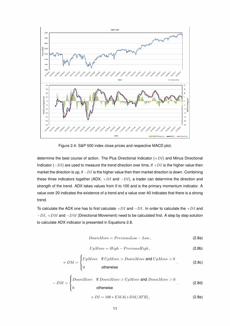
Figure 2.4: S&P 500 index close prices and respective MACD plot.
determine the best course of action. The Plus Directional Indicator (+DI) and Minus Directional
Indicator (−DI) are used to measure the trend direction over time, if +DI is the higher value then
market the direction is up, if−DI is the higher value then then market direction is down. Combining
these three indicators together (ADX, +DI and −DI), a trader can determine the direction and
strength of the trend. ADX takes values from 0 to 100 and is the primary momentum indicator. A
value over 20 indicates the existence of a trend and a value over 40 indicates that there is a strong
trend.
To calculate the ADX one has to first calculate +DI and −DI. In order to calculate the +DI and
−DI, +DM and −DM (Directional Movement) need to be calculated first. A step by step solution
to calculate ADX indicator is presented in Equations 2.8.
DownMove = PreviousLow − Low , (2.8a)
UpMove = High− PreviousHigh , (2.8b)
+DM =
UpMove if UpMove > DownMove and UpMove > 0
0 otherwise. (2.8c)
−DM =
DownMove if DownMove > UpMove and DownMove > 0
0 otherwise. (2.8d)
+DI = 100 ∗ EMA(+DM/ATR) , (2.8e)
11
−DI = 100 ∗ EMA(−DM/ATR) , (2.8f)
ADX = 100 ∗ EMA(
∣∣∣∣ (+DI)− (−DI)
(+DI) + (−DI)
∣∣∣∣) . (2.8g)
• Momentum
Momentum is an oscillator used to help in identifying trend lines, and can be seen as the rate of
acceleration of a stock’s price or volume, i.e it refers to the rate of change on price movements
of a stock. Due to the fact that there are more times when the market is rising than when the
market is falling, momentum has proven to be more useful during rising markets. The formula
used to calculate the momentum indicator is presented in Equation 2.9, where Closen represents
the close price n days ago.
Momentum = Close− Closen (2.9)
• Commodity Channel Index (CCI)
The Commodity Channel Index (CCI) is an indicator that can be used to identify a new trend
and to identify overbought and oversold levels by measuring the current price level relative to an
average price level over a given period of time. CCI is relatively high when prices are far above
their average, conversely it takes relatively low values when prices are far below their average.
The formulas used to calculate the CCI indicator are presented in Equation 2.10, where MD
represents the mean deviation of prices over the last 20 days.
CCI =TP − SMA20(TP )
0.015 ∗MD
with TP =High+ Low + Close
3(2.10)
• Rate of Change (ROC)
The Rate of Change (ROC) is a momentum technical indicator that measures the percent change
in price between the current period relatively to n periods ago. A positive ROC usually means that
the stock’s price will increase and can be seen as a buy signal to investors. Conversely, a stock
that has a negative ROC is likely to decline in value and can be seen as a sell signal. If a stock
has a positive ROC above 30 this indicates that it is overbought, if it has a negative ROC below
-30 this indicates that it is oversold. The formula used to calculate the ROC indicator is presented
in Equation 2.11.
ROC =Close− Closen
Closen∗ 100 (2.11)
12
• Stochastic
The Stochastic Oscillator is a momentum indicator that shows the location of the close relative to
the high-low range over a set number of periods. This indicator attempts to predict price turning
points by comparing the closing price of a security to its price range. Values above 80 for the
Stochastic Oscillator indicate that the security was trading near the top of its high-low range for the
given period of time. Values below 20 occur when a security is trading at the low end of its high-
low range for the given period of time. Usually these values are also used to identify overbought
and oversold conditions, being 80 the overbought threshold and 20 the oversold threshold. A
transaction signal is created once the Stochastic %K crosses its 3-period moving average, which
is called the Stochastic %D. The formulas used to calculate the Stochastic %D and %K indicators
are presented in Equation 2.12.
%K =Close− LowestLow
HighestHigh− LowestLow∗ 100 , (2.12a)
%D = SMA3(%K) . (2.12b)
• William’s %R
The William’s %R is a momentum indicator that compares the close price of a stock to the high-low
range over a period of time. Due to its usefulness in signalling market reversals at least one to
two periods in the future, it is used not only to anticipate market reversals, but also to determine
overbought and oversold conditions. Williams %R ranges from -100 to 0. When its value is above
-20, it indicates a sell signal and when its value is below -80, it indicates a buy signal. Readings
from 0 to -20 represent overbought conditions and readings from -80 to -100 represent oversold
conditions. The formula used to calculate the William’s %R indicator is presented in Equation 2.13.
%R =HighestHigh− Close
HighestHigh− LowestLow∗ (−100) (2.13)
Volume
Volume indicators combine the basic volume with the stock price and are used to confirm the strength of
price movements to determine if a stock is gaining or losing momentum. The volume indicators that will
be used in this thesis are On Balance Volume (OBV), Money Flow Index (MFI) and the Chaikin Oscillator.
• On Balance Volume (OBV)
On balance volume (OBV) is a momentum indicator that uses volume flow to predict changes in a
stock’s price by measuring buying and selling pressure as a cumulative indicator that adds volume
on up days and subtracts it on down days. The main idea behind this indicator is that if volume
increases very quickly and the stock’s price doesn’t change that much, it means that sooner or
later the stock’s price will go up, and vice versa. The OBV line is a running total of positive and
13
negative volume. A period’s volume is positive when the close is above the previous close and
negative when the close is below the previous close.
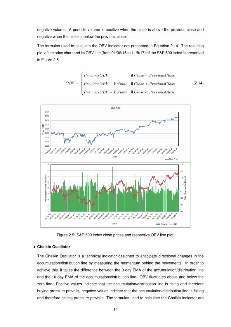
The formulas used to calculate the OBV indicator are presented in Equation 2.14. The resulting
plot of the price chart and its OBV line (from 01/06/15 to 11/8/17) of the S&P 500 index is presented
in Figure 2.5.
OBV =
PreviousOBV if Close = PreviousClose
PreviousOBV + V olume if Close > PreviousClose
PreviousOBV − V olume if Close < PreviousClose
(2.14)
Figure 2.5: S&P 500 index close prices and respective OBV line plot.
• Chaikin Oscillator
The Chaikin Oscillator is a technical indicator designed to anticipate directional changes in the
accumulation/distribution line by measuring the momentum behind the movements. In order to
achieve this, it takes the difference between the 3-day EMA of the accumulation/distribution line
and the 10-day EMA of the accumulation/distribution line. OBV fluctuates above and below the
zero line. Positive values indicate that the accumulation/distribution line is rising and therefore
buying pressure prevails, negative values indicate that the accumulation/distribution line is falling
and therefore selling pressure prevails. The formulas used to calculate the Chaikin indicator are
14
presented in Equations 2.15.
MoneyF lowMultiplier =(Close− Low)− (High− Close)
High− Low, (2.15a)
MoneyF lowV olume = MoneyF lowMultiplier ∗ V olume , (2.15b)
ADL = PreviousADL+MoneyF lowV olume , (2.15c)
Chaikin = EMA3(ADL)− EMA10(ADL) . (2.15d)
• Money Flow Index (MFI)
The Money Flow Index (MFI) is a momentum indicator that measures the buying and selling pres-
sure by using both the stock’s price and volume and is best suited to identify reversals and price
extremes. Money flow is positive when the typical price rises (buying pressure) and negative when
the typical price declines (selling pressure). When the MFI moves in the opposite direction as
the price this usually indicates that there is a change in the current trend. MFI takes values be-
tween 0 and 100. An MFI above 80 suggests the security is overbought, while a value lower than
20 suggests the security is oversold. The formulas used to calculate the MFI indicator are pre-
sented in Equations 2.16, being PositiveMoneyF low and NegativeMoneyF low the sum of the
RawMoneyF low in the look-back period (14 days) for up and down days, respectively.
TypicalPrice =High+ Low + Close
3, (2.16a)
RawMoneyF low = TypicalPrice ∗ V olume , (2.16b)
MoneyF lowRatio =14period PositiveMoneyF low
14period NegativeMoneyF low, (2.16c)
MFI = 100− 100
1 +MoneyF lowRatio. (2.16d)
Volatility
Volatility refers to the uncertainty associated with the stock’s price. An highly volatile stock is a stock
whose price can change dramatically over a short time period in either direction, being a riskier invest-
ment due to its unpredictable behaviour, however the risk of failure is just as high as the risk of success.
A lowly volatile stock is a stock whose price is relatively stable. The volatility technical indicator used in
this thesis is the Average True Range (ATR).
• Average True Range (ATR)
The Average True Range (ATR) is an indicator that measures the volatility present in the market. A
stock experiencing a high level of volatility has a higher ATR, conversely a stock experiencing a low
15

level of volatility has a lower ATR. This indicator does not provide an indication about the direction
of the stock’s price, but extremes in activity can indicate a change in a stock’s movement i.e, an
higher ATR value can mean a stock is trending and there is an high market volatility, and a lower
ATR value could indicate a consolidation in price and a lower market volatility. The formula used to
calculate the ATR indicator is presented in Equation 2.17, where TR represents the greatest of the
true range indicators. The first ATR value is the average of the daily TR values for the last 14-day
period.
ATR =PreviousATR ∗ 13 + TR
14
with TR = maxHigh− Low, |High− PreviousClose| , |Low − PreviousClose| (2.17)
2.1.3 Machine Learning
The utilization of Machine Learning methods in financial markets is done in an attempt to develop al-
gorithms capable of learning from historical financial data and other information that might affect the
market and make predictions based on these inputs in order to try to maximize the returns. At this mo-
ment, Machine Learning methods have already progressed enough that they can be extremely useful in
predicting the evolution of a stock price. This is due to the fact that Machine Learning algorithms can
process data at a much larger scale and with much larger complexity, discovering relationships between
features that may be incomprehensible to humans. Therefore, by exploiting the relationships between
the input data, consisting of historical raw financial data as well as technical indicators, and learning
from it, these models make predictions about the behaviour of a stock price that can be used in order to
create a trading strategy capable of obtaining high returns.
2.2 Principal Component Analysis
Having a data set of large dimensions can often be a problem due to the fact that it may lead to higher
computational costs and to overfitting. Therefore one may want to reduce the data set dimension in
order to make the data manipulation easier and lower the required computational resources, improving
the performance of the system and while keeping as much information as possible from the original data.
Principal Component Analysis (PCA) is one of the simplest and most used dimensionality reduction
methods and can be used to reduce a data set with a large number of dimensions to a small data set
that still contains most of the information of the original data set. This is done by transforming the original
features to a new set of uncorrelated features, known as principal components, ordered such that the
retention of variance present in the original features decreases as the order of the principal component
decreases. In this way, this means that the first principal component retains the maximum variance that
was present in the original data set. By performing this transformation, a low dimensional representation
of the original data is achieved while keeping its maximal variance.
16

The purpose of the PCA is to make a projection from the main components of an high-dimensional
data set onto a lower dimensional space, without changing the data structure, and obtaining a set of
principal components that are a linear combination of the features present in the original data set that
reflect its information as much as possible. As already discussed, this transformation is done in a
way that the first principal component has the largest variance possible and each succeeding principal
component will have the highest possible variance, under the condition that each principal component
must be orthogonal to the ones preceding it, since they are eigenvectors of a covariance matrix and the
eigenvectors are mutually orthogonal.
The goal is to retain the dimensions with high variances and remove those with little changes in
order to reduce the required computational resources [3], which results in a set of principal components
that has the same dimension of the original data set or lower in the case of performing dimensionality
reduction since only the principal components that retain most of the original data set variance will be
retained. Importantly, the data set on which the PCA technique is applied must be scaled, with the
results being also sensitive to the relative scaling.
The steps required in order to apply PCA to a given data set X are:
1. Since in PCA the interest lies in the variation of the data about the mean, it is important to first
center the data. Therefore, for each column of the matrix X, for each entry of the matrix the mean
of that column is subtracted to it, in order to ensure that each column has a mean of zero. This
centered matrix X is now called X∗. The next step is to calculate the covariance matrix, Cov(X∗),
of the original data set X∗ with dimension n x n, where n is the dimension of the data set X∗. The
covariance matrix is a matrix that contains estimates of how every variable in X∗ relates to every
other variable in X∗;
2. Obtain the matrix of eigenvectors, W , and their corresponding eigenvalues, λ, of the covariance
matrix Cov(X∗). This can be done by solving the eigenproblem represented in Equation 2.18.
Cov(X∗) ∗W = λ ∗W (2.18)
The matrixW contains n eigenvectors of dimension n. These eigenvectors of Cov(X∗) correspond
to the directions with the greatest variance of the data, meaning that they represent the principal
components of the original data set. The eigenvalues represent the magnitude or importance of
the corresponding eigenvector, i.e the bigger the eigenvalue, the more important is the direction
of the corresponding eigenvector. By sorting the eigenvalues λ in descending order, it is possible
to rank the eigenvectors in an order of significance based on how much variance each principal
component retains from the original data set. This new sorted matrix of eigenvectors is called
W ∗, it has the same columns of W but with a different order. The first m principal directions of
the original data set are the directions of the eigenvectors of W ∗ that correspond to the m largest
eigenvalues [4];
3. Project the data set X∗ onto the new space formed by the eigenvectors present in W ∗. This is
17

done using Equation 2.19, where Z is a centered version of X but where each observation is a
combination of the original variables where the weights are determined by the eigenvectors;
Z = X∗ ∗W ∗ (2.19)
4. The last step is to determine how many features (principal components) from Z to keep. In order
to do so, the user can determine how many features to keep or specify a threshold of explained
variance to achieve and add features until the threshold is hit. In this thesis, the second method
is used and a threshold of 95% of explained variance is chosen. The features with the largest
explained proportion of variance will be added, one at a time, until the total proportion of explained
variance reaches 95%.
In figure 2.6 a practical example of the application of PCA to a multivariate Gaussian data set is
presented. The first principal component is represented by the red arrow and the second principal
component is represented by the green arrow. The reason why there are only two principal components
represented in figure 2.6 is because any other component of the data set would have some component
of the red or green arrow i.e, if there were any other arrows they would have to be correlated with either
the red, the green or both arrows which goes against the PCA method that transforms a data set of
possible correlated variables into a data set of linearly uncorrelated variables.
Figure 2.6: Plot of the two principal components in the data set.
Once the principal components in the data set are determined, the data can be projected on the
principal components obtained. This projection is presented in figure 2.7. In this new space, the data
points are uncorrelated and the principal components are now aligned with the coordinate axes.
What was done in this example using the PCA method was represent the original data set using the
18
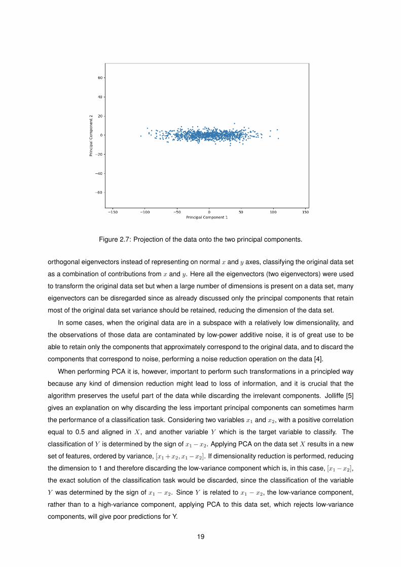
Figure 2.7: Projection of the data onto the two principal components.
orthogonal eigenvectors instead of representing on normal x and y axes, classifying the original data set
as a combination of contributions from x and y. Here all the eigenvectors (two eigenvectors) were used
to transform the original data set but when a large number of dimensions is present on a data set, many
eigenvectors can be disregarded since as already discussed only the principal components that retain
most of the original data set variance should be retained, reducing the dimension of the data set.
In some cases, when the original data are in a subspace with a relatively low dimensionality, and
the observations of those data are contaminated by low-power additive noise, it is of great use to be
able to retain only the components that approximately correspond to the original data, and to discard the
components that correspond to noise, performing a noise reduction operation on the data [4].
When performing PCA it is, however, important to perform such transformations in a principled way
because any kind of dimension reduction might lead to loss of information, and it is crucial that the
algorithm preserves the useful part of the data while discarding the irrelevant components. Jolliffe [5]
gives an explanation on why discarding the less important principal components can sometimes harm
the performance of a classification task. Considering two variables x1 and x2, with a positive correlation
equal to 0.5 and aligned in X, and another variable Y which is the target variable to classify. The
classification of Y is determined by the sign of x1−x2. Applying PCA on the data set X results in a new
set of features, ordered by variance, [x1 +x2, x1−x2]. If dimensionality reduction is performed, reducing
the dimension to 1 and therefore discarding the low-variance component which is, in this case, [x1−x2],
the exact solution of the classification task would be discarded, since the classification of the variable
Y was determined by the sign of x1 − x2. Since Y is related to x1 − x2, the low-variance component,
rather than to a high-variance component, applying PCA to this data set, which rejects low-variance
components, will give poor predictions for Y.
19

Many studies regarding the stock market have used PCA in order to improve the performance of the
system. He et. al [3] studied three kinds of feature selection algorithms in order to find out in a set of
technical indicators which were the most important in their analysis model, and concluded that PCA is
the most reliable and accurate method. Zhong et. al [6] proposed a system combining Artificial Neural
Networks (ANN) and three different dimensionality reduction methods, PCA, Fast Robust PCA (FRPCA)
and Kernel PCA (KPCA), in order to forecast the daily direction of the S&P 500 Index ETF (SPY) and
concluded that combining the ANN with the PCA gives higher classification accuracy than the other two
combinations. Nadkarni [7] concluded that the PCA method for dimensionality reduction can reduce the
number of features while maintaining the essence of the financial data, improving the performance of the
NEAT algorithm. Furthermore, Weng [8] compared the performance of three methods, Neural Network,
Support Vector Machine and Boosted Trees in order to predict short-term stock price and concluded that
all three models have better performance on accuracy if trained with PCA transformed predictors and
that specially without PCA transformation, boosting also has test errors more than three times as large
as those with PCA.
A more extensive description about PCA can be found in [9].
2.3 Wavelet Transform
Fourier transform based spectral analysis is the most used tool for an analysis in the frequency domain.
According to Fourier theory, a signal can be expressed as the sum of a series of sines and cosines, as
can be observed in the Fourier Transform expression presented in Equation 2.20.
F (w) =
∫ +∞
−∞f(t)e−jwtdt =
∫ +∞
−∞f(t)(cos(wt)− jsin(wt))dt (2.20)
However, a serious limitation of the Fourier transform is that it cannot provide any information of the
spectrum changes with respect to time. Therefore, although we can identify all the frequencies present
in a signal, we do not know the time instants in which they are present. To overcome this problem, the
wavelet theory is proposed. The wavelet transform is similar to the Fourier transform but with a different
merit function. The main difference is that instead of decomposing the signal into sines and cosines, the
wavelet transform uses functions that are localized in both time and frequency.
The basic idea of the wavelet transform is to represent any function as a superposition of a set of
wavelets that constitute the basis function for the wavelet transform. A wavelet is a function with zero
average, as represented in Equation 2.21.
∫ +∞
−∞ψ(t)dt = 0 (2.21)
These functions are small waves located in different times and can be stretched and shifted to cap-
ture features that are local in time and local in frequency, therefore the wavelet transform can provide
information about both the time and frequency domains in a signal.
20
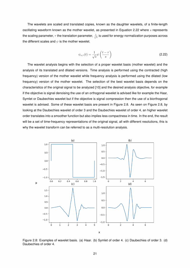
The wavelets are scaled and translated copies, known as the daughter wavelets, of a finite-length
oscillating waveform known as the mother wavelet, as presented in Equation 2.22 where s represents
the scaling parameter, τ the translation parameter, 1√s
is used for energy normalization purposes across
the different scales and ψ is the mother wavelet.
ψs,τ (t) =1√sψ
(t− τs
)(2.22)
The wavelet analysis begins with the selection of a proper wavelet basis (mother wavelet) and the
analysis of its translated and dilated versions. Time analysis is performed using the contracted (high
frequency) version of the mother wavelet while frequency analysis is performed using the dilated (low
frequency) version of the mother wavelet. The selection of the best wavelet basis depends on the
characteristics of the original signal to be analyzed [10] and the desired analysis objective, for example
if the objective is signal denoising the use of an orthogonal wavelet is advised like for example the Haar,
Symlet or Daubechies wavelet but if the objective is signal compression then the use of a biorthogonal
wavelet is advised. Some of these wavelet basis are present in Figure 2.8. As seen on Figure 2.8, by
looking at the Daubechies wavelet of order 3 and the Daubechies wavelet of order 4, an higher wavelet
order translates into a smoother function but also implies less compactness in time. In the end, the result
will be a set of time-frequency representations of the original signal, all with different resolutions, this is
why the wavelet transform can be referred to as a multi-resolution analysis.
Figure 2.8: Examples of wavelet basis. (a) Haar. (b) Symlet of order 4. (c) Daubechies of order 3. (d)Daubechies of order 4.
21

There are two types of wavelet transform, the Continuous Wavelet Transform (CWT) and the Discrete
Wavelet Transform (DWT).
2.3.1 Continuous Wavelet Transform
In the CWT the input signal is convolved with the continuous mother wavelet chosen for the analysis.
While the Fourier transform decomposes the signal into a the sum of sines and cosines with different
frequencies, the Continuous Wavelet Transform breaks down the signal into a set of wavelets with differ-
ent scales and translations. Therefore, the CWT generalizes the Fourier transform but unlike the latter,
has the advantage to detect seasonal oscillations with time-varying intensity and frequency [11].
The Continuous Wavelet Transform of a signal f(t) at scale s and time τ can be expressed by the
formula present in Equation 2.23, where * denotes the complex conjugation and the variables s and τ
represent the new dimensions, i.e. scale and translation, after the wavelet transform.
Wf(s, τ) =
∫ +∞
−∞f(t)ψ∗s,τ (t)dt =
∫ +∞
−∞f(t)
1√sψ∗(t− τs
)dt (2.23)
The CWT will not be expanded more in this thesis because calculating and storing the CWT coeffi-
cients at every possible scale can be very time consuming and requires an high computational cost and
besides that, the results can be difficult to analyze due to the redundancy of the CWT. Instead the DWT
will be used since the analysis is more accurate and faster.
2.3.2 Discrete Wavelet Transform
To overcome the already discussed inefficiencies of the CWT, the DWT is presented. Unlike the CWT,
the DWT decomposes the signal into a set of wavelets that is mutually orthogonal. The discrete wavelet
is related to the mother wavelet [12] as presented in Equation 2.24, where the parameter m is an integer
that controls the wavelet dilation, the parameter k is an integer that controls the wavelet translation, s0
is a fixed scaling parameter set at a value greater than 1, τ0 is the translation parameter which has to be
greater than zero and ψ is the mother wavelet.
ψm,k(t) =1√sm0
ψ
(t− kτ0sm0
sm0
)(2.24)
The CWT and the DWT differ in the way the scaling parameter is discretized. While the CWT typically
uses exponential scales with a base smaller than 2, the DWT always uses exponential scales with a
base equal to 2. By making s0 = 2 and τ0 = 1, a dyadic sampling of the frequency axis is achieved [12]
and allows viewing the wavelet decomposition as a tree-structured discrete filter bank. The dyadic grid
wavelet expression is present in Equation 2.25.
ψm,k(t) =1√2m
ψ
(t− k ∗ 2m
2m
)= 2−m/2ψ(2−mt− k) (2.25)
An algorithm to calculate the DWT was developed by Mallat [13], using a process that is equivalent to
22
high-pass and low-pass filtering in order to obtain the detail and approximation coefficients, respectively,
from the original signal. The output of each analysis filter is downsampled by a factor of two. Each
low-pass sub-band produced by the previous transform is then subdivided into its own high-pass and
low-pass sub-bands by the next level of the transform. Each iteration of this process is called a level of
decomposition, and it is common to choose small levels of decomposition since nearly all the energy
of the coefficients is concentrated in the lower sub-bands [14]. This process produces one approxi-
mation coefficient and j detail coefficients, with j being the chosen decomposition level. The reason
why only one approximation coefficient is obtained, which is the one corresponding to the last level of
decomposition, is because the approximation coefficient at each level of decomposition, except the last
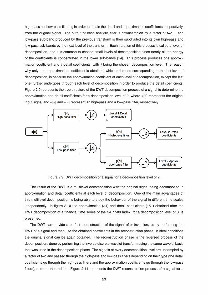
one, further undergoes through each level of decomposition in order to produce the detail coefficients.
Figure 2.9 represents the tree structure of the DWT decomposition process of a signal to determine the
approximation and detail coefficients for a decomposition level of 2, where x[n] represents the original
input signal and h[n] and g[n] represent an high-pass and a low-pass filter, respectively.
Figure 2.9: DWT decomposition of a signal for a decomposition level of 2.
The result of the DWT is a multilevel decomposition with the original signal being decomposed in
approximation and detail coefficients at each level of decomposition. One of the main advantages of
this multilevel decomposition is being able to study the behaviour of the signal in different time scales
independently. In figure 2.10 the approximation (cA) and detail coefficients (cDj) obtained after the
DWT decomposition of a financial time series of the S&P 500 Index, for a decomposition level of 3, is
presented.
The DWT can provide a perfect reconstruction of the signal after inversion, i.e by performing the
DWT of a signal and then use the obtained coefficients in the reconstruction phase, in ideal conditions
the original signal can be again obtained. The reconstruction phase is the reversed process of the
decomposition, done by performing the inverse discrete wavelet transform using the same wavelet basis
that was used in the decomposition phase. The signals at every decomposition level are upsampled by
a factor of two and passed through the high-pass and low-pass filters depending on their type (the detail
coefficients go through the high-pass filters and the approximation coefficients go through the low-pass
filters), and are then added. Figure 2.11 represents the DWT reconstruction process of a signal for a
23
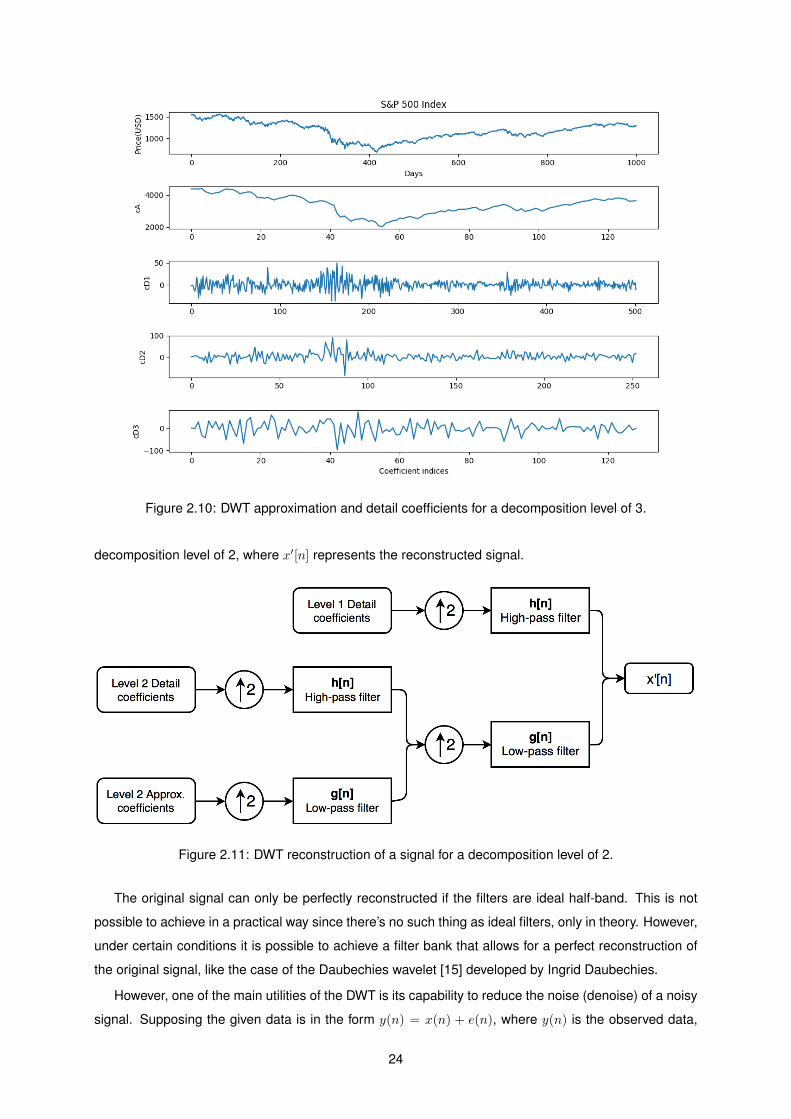
Figure 2.10: DWT approximation and detail coefficients for a decomposition level of 3.
decomposition level of 2, where x′[n] represents the reconstructed signal.
Figure 2.11: DWT reconstruction of a signal for a decomposition level of 2.
The original signal can only be perfectly reconstructed if the filters are ideal half-band. This is not
possible to achieve in a practical way since there’s no such thing as ideal filters, only in theory. However,
under certain conditions it is possible to achieve a filter bank that allows for a perfect reconstruction of
the original signal, like the case of the Daubechies wavelet [15] developed by Ingrid Daubechies.
However, one of the main utilities of the DWT is its capability to reduce the noise (denoise) of a noisy
signal. Supposing the given data is in the form y(n) = x(n) + e(n), where y(n) is the observed data,
24
x(n) is the original data and e(n) is Gaussian white noise with zero mean and variance σ2, the main
objective of denoising the data is to reduce the noise as much as possible and recover the original data
x(n) with as little loss of important information as possible. The main steps to reduce the noise present
in the data using the DWT are the following:
1. Select the wavelet basis, order and the level of decomposition to be used;
2. Choose the threshold value and apply the selected thresholding method to the detail coefficients,
since noise is assumed to be mostly present in the detail coefficients [16], in each decomposition
level;
3. Perform the inverse discrete wavelet transform using only the set of coefficients obtained after the
thresholding process in order to obtain a denoised reconstruction of the original signal.
The important features of many signals are captured by a subset of DWT coefficients that is typically
much smaller than the original signal itself. This is because when performing the DWT, the same number
of coefficients than the original signal is obtained but many of them may be very small and therefore
irrelevant. By thresholding all the coefficients, one can choose the subset of relevant coefficients that
will be kept after the DWT.
The two most used methods in order to determine the tresholding values are the universal thresh-
old, proposed by Donoho and Johnstone and incorporated in their VisuShrink method [17] and the
BayesShrink method, proposed by Chang et. al [18]. While in the VisuShrink approach a single uni-
versal threshold is applied to all wavelet detail coefficients, in the BayesShrink approach an unique
threshold is estimated for each wavelet subband, resulting often in better results compared to what
can be obtained with a single threshold. Due to the advantages of using the BayesShrink approach to
determine the thresholding values, it will be used in this thesis.
The formula used to calculate the threshold using the BayesShrink method is presented in Equation
2.26, where σ is an estimate of the noise level σ that can be calculated using the formula presented in
Equation 2.27, as proposed by Chang et. al in [18], where Median|Yij | is the median of all the discrete
wavelet coefficients of the detail sub-band in consideration and σX is the standard deviation of the signal,
X.
TB(σX) =σ2
σX(2.26)
σ =Median|Yij |
0.6745(2.27)
Recalling that the observation model is of the type Y = X + E, then σ2Y = σ2
X + σ2 and thus
the formula used to calculate σX is the one presented in Equation 2.28, where σ2Y is calculated using
Equation 2.29, with n being the number of detail coefficients in the sub-band in consideration.
σX =√max(σ2
Y − σ2, 0) (2.28)
25
σ2Y =
1
n2
n∑i,j=1
Y 2ij (2.29)
Given the threshold value and the discrete wavelet coefficients, in order to suppress the noise what
remains is to choose how the discrete wavelet coefficients should be modified. Donoho et. al [19]
propose the shrinkage process by thresholding the coefficients, in which a hard or a soft threshold value
must be chosen. When performing hard thresholding, all the coefficients smaller than the threshold value
are set to zero while if soft thresholding is used, the values for both positive and negative coefficients are
shrinked towards zero. The formulas used to calculate hard or soft thresholding values are presented in
Equation 2.30 and Equation 2.31, respectively, where w is the discrete wavelet coefficient and λ is the
threshold value, with λ > 0.
Tλ(w) =
0 if |w| ≤ λ
w otherwise. (2.30)
Tλ(w) =
w − λ if w > λ
0 if |w| ≤ λ
w + λ if w < −λ
. (2.31)
Although there is not much theory about which thresholding method is better, due to the fact that
when using soft thresholding the results are smoother and the noise is almost fully suppressed [19] in
comparison to the hard thresholding, in this thesis soft threshold will be applied. After that process the
result will be a new set of DWT coefficients already thresholded, used in the inverse DWT to reconstruct
the original signal. By discarding these irrelevant coefficients and only using the coefficients that capture
the important features of the original signal in the reconstruction phase, the result will be a denoised
signal with the main features of the original signal.
Due to its favorable properties, the wavelet analysis provides a way to deal with time varying char-
acteristics found in most of the real world problems involving time series like the stock market, where
the assumption of stationarity may not be applied. Hsieh et. al [20] proposed a system based on re-
current neural network (RNN) and artificial bee colony (ABC) algorithm for stock price forecasting where
the data preprocessing was done using the Haar wavelet is to decompose the stock price time series
and eliminate the noise and concluded that the wavelet-based preprocessing approach greatly outper-
forms other methods compared by the authors in TAIEX index. M’ng and Mehralizadeh [21] proposed
an hybrid model WPCA-RNN which combines the wavelet transform and PCA techniques to perform a
multivariate denoising, together with a RNN in order to forecast the stock market and concluded that
using the wavelet transform together with the PCA technique proves to be a more successful approach
when reducing the noise in the input features and allows for greater returns than using just the neural
network or using the neural network together with the wavelet transform as a denoising method.
A more extensive description about the wavelet transform can be found in [22].
26
2.4 Extreme Gradient Boosting
In Machine Learning, boosting [23] is an ensemble technique that attempts to create a strong learner
from a given number of weak learners, i.e models that only perform slightly better than random guessing.
An ensemble is a set of predictors, all trying to predict the same target variable, which are combined
together in order to give a final prediction. The use of ensemble methods allows for a better predictive
performance compared to a single predictor alone by helping in reducing the bias and variance in the
predictions [24], this way reducing the prediction error. This process is done by creating a model from
the training data, then creating a second model which will try to correct the errors from the first model
and so forth, until an high accuracy value is achieved or the maximum number of models is added. In the
end, it combines the outputs of every weak learner in order to create a strong learner which is expected
to improve the prediction performance of the model. In the case of classification problems, the results
of the weak classifiers are combined and the classification of the test data is done by taking a weighted
vote of each weak classifier’s prediction.
The main principle of boosting is to iteratively fit a sequence of weak learners to weighted versions
of the training data. After each iteration, more weight is given to training samples that were misclassified
by earlier rounds. In the end of the process, all of the successive models are weighted according to
their performance and the outputs are combined using voting for classification problems or averaging for
regression problems, creating the final model.
Since boosting reduces both bias and variance in the predictions, due to the particular characteristic
of individual decision trees of having an high variance in terms of generalization accuracy, by using
the boosting approach together with decision trees the performance of the model can be improved by
lowering variance. The first successful application of boosting was AdaBoost [25], short for Adaptive
Boosting. In AdaBoost less weights are given to strong learners, while more weights are given to the
weak learners. This weights are constantly changed until the performance of the model is at the level
desired by the user.
XGBoost [26], short for Extreme Gradient Boosting, is a machine learning system based on Fried-
man’s [27] Gradient Boosting. The Gradient Boosting method can be seen as the combination of the
Gradient Descent method and boosting, and is performed as follows:
1. A differentiable loss function is chosen according to the characteristics of the problem to be solved,
this can be for example the Mean Squared Error (MSE), Logarithmic Loss, Area Under the Curve
(AUC);
2. A weak learner is created in order to make the predictions. In Gradient Boosting a common base-
learner is the decision tree, constructed in a greedy manner and choosing the best split points in
order to minimize the loss function. The model is fitted on the training data and the error residuals
are calculated, i.e the target value minus the predicted target value. These errors represent the
data points that the model found more difficult to fit;
3. A new model is created and fitted in the residuals, i.e the new model will focus on classifying
27
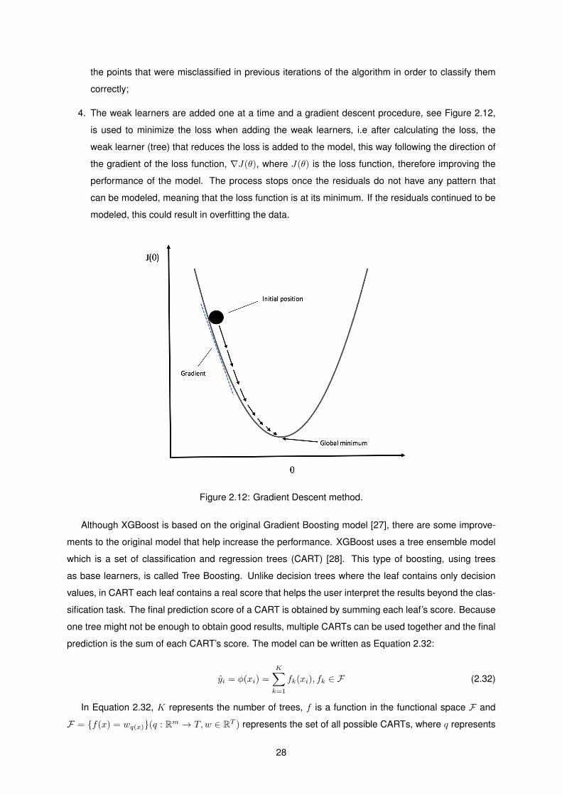
the points that were misclassified in previous iterations of the algorithm in order to classify them
correctly;
4. The weak learners are added one at a time and a gradient descent procedure, see Figure 2.12,
is used to minimize the loss when adding the weak learners, i.e after calculating the loss, the
weak learner (tree) that reduces the loss is added to the model, this way following the direction of
the gradient of the loss function, ∇J(θ), where J(θ) is the loss function, therefore improving the
performance of the model. The process stops once the residuals do not have any pattern that
can be modeled, meaning that the loss function is at its minimum. If the residuals continued to be
modeled, this could result in overfitting the data.
Figure 2.12: Gradient Descent method.
Although XGBoost is based on the original Gradient Boosting model [27], there are some improve-
ments to the original model that help increase the performance. XGBoost uses a tree ensemble model
which is a set of classification and regression trees (CART) [28]. This type of boosting, using trees
as base learners, is called Tree Boosting. Unlike decision trees where the leaf contains only decision
values, in CART each leaf contains a real score that helps the user interpret the results beyond the clas-
sification task. The final prediction score of a CART is obtained by summing each leaf’s score. Because
one tree might not be enough to obtain good results, multiple CARTs can be used together and the final
prediction is the sum of each CART’s score. The model can be written as Equation 2.32:
yi = φ(xi) =
K∑k=1
fk(xi), fk ∈ F (2.32)
In Equation 2.32, K represents the number of trees, f is a function in the functional space F and
F = f(x) = wq(x)(q : Rm → T,w ∈ RT ) represents the set of all possible CARTs, where q represents
28
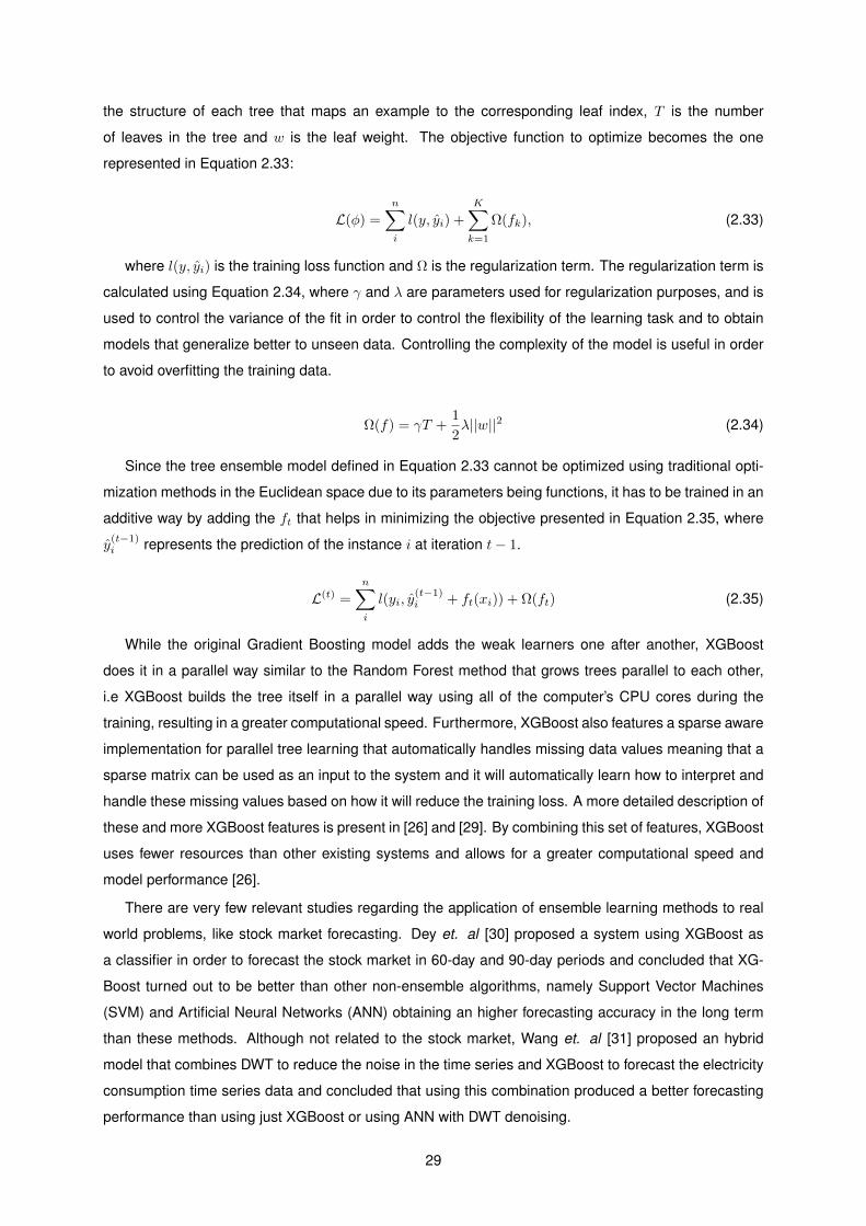
the structure of each tree that maps an example to the corresponding leaf index, T is the number
of leaves in the tree and w is the leaf weight. The objective function to optimize becomes the one
represented in Equation 2.33:
L(φ) =
n∑i
l(y, yi) +
K∑k=1
Ω(fk), (2.33)
where l(y, yi) is the training loss function and Ω is the regularization term. The regularization term is
calculated using Equation 2.34, where γ and λ are parameters used for regularization purposes, and is
used to control the variance of the fit in order to control the flexibility of the learning task and to obtain
models that generalize better to unseen data. Controlling the complexity of the model is useful in order
to avoid overfitting the training data.
Ω(f) = γT +1
2λ||w||2 (2.34)
Since the tree ensemble model defined in Equation 2.33 cannot be optimized using traditional opti-
mization methods in the Euclidean space due to its parameters being functions, it has to be trained in an
additive way by adding the ft that helps in minimizing the objective presented in Equation 2.35, where
y(t−1)i represents the prediction of the instance i at iteration t− 1.
L(t) =
n∑i
l(yi, y(t−1)i + ft(xi)) + Ω(ft) (2.35)
While the original Gradient Boosting model adds the weak learners one after another, XGBoost
does it in a parallel way similar to the Random Forest method that grows trees parallel to each other,
i.e XGBoost builds the tree itself in a parallel way using all of the computer’s CPU cores during the
training, resulting in a greater computational speed. Furthermore, XGBoost also features a sparse aware
implementation for parallel tree learning that automatically handles missing data values meaning that a
sparse matrix can be used as an input to the system and it will automatically learn how to interpret and
handle these missing values based on how it will reduce the training loss. A more detailed description of
these and more XGBoost features is present in [26] and [29]. By combining this set of features, XGBoost
uses fewer resources than other existing systems and allows for a greater computational speed and
model performance [26].
There are very few relevant studies regarding the application of ensemble learning methods to real
world problems, like stock market forecasting. Dey et. al [30] proposed a system using XGBoost as
a classifier in order to forecast the stock market in 60-day and 90-day periods and concluded that XG-
Boost turned out to be better than other non-ensemble algorithms, namely Support Vector Machines
(SVM) and Artificial Neural Networks (ANN) obtaining an higher forecasting accuracy in the long term
than these methods. Although not related to the stock market, Wang et. al [31] proposed an hybrid
model that combines DWT to reduce the noise in the time series and XGBoost to forecast the electricity
consumption time series data and concluded that using this combination produced a better forecasting
performance than using just XGBoost or using ANN with DWT denoising.
29

2.5 Genetic Algorithm
A genetic algorithm (GA) is a meta-heuristic algorithm for optimization that belongs to the area of Evo-
lutionary Computation, inspired by natural processes like evolution, survival and adaptation to the en-
vironment. The GA, first introduced by Holland [32] is used to effectively search complex spaces for
an optimal solution to a given optimization problem. It is based on Darwin’s principle ”survival of the
fittest” and draws its inspiration on the biological processes of evolution more specifically reproduction,
crossover and mutation in order to produce solutions which become better adapted to the environment
they are inserted in, i.e solutions that continuously perform better at the desired optimization task.
A GA is composed by a set of individuals (the different candidate solutions) called population. Each
individual, called chromosome, is evaluated according to a fitness function that reflects the performance
of the individual, i.e its fitness in the given optimization task. Each parameter to be optimized on the
chromosome is called the gene.
The first step in the GA is to create an initial random population, i.e with each gene of a chromosome
taking random values in a given interval defined by the user. After all the chromosomes have their genes
defined, the initial population is created and the following steps are taken in each generation:
1. Evaluation: Each chromosome of the population is evaluated and a fitness value is assigned
according to its performance at the given optimization task;
2. Selection: Some of the individuals are selected for reproduction, with the individuals with an higher
fitness being more likely to be chosen in order to guarantee that the genetic algorithm will evolve
towards better solutions at each generation;
3. Crossover: The selected individuals are then combined creating an offspring with some features
of each parent, i.e the offspring’s genes are a combination of its parents genes. The purpose of
crossover is to generate better performing candidate solutions since each new candidate solution
resulting from the crossover retains the best features of its parents, that were two of the best
performing solutions of the previous generation. Two ways of applying the crossover operator are
Single-Point Crossover and Two-Point Crossover. In Single-Point Crossover, one crossover point is
selected on both parents’ strings and all data beyond that point in either parent’s string is swapped
between the two parents. In Two-Point Crossover, two points are selected on the parent’s strings
and everything between the two selected points is swapped between the parents. These two
methods are represented in Figure 2.13. In this thesis, the crossover operator chosen is Two-Point
Crossover. Crossover occurs during the evolution according to a crossover rate defined by the
user. In this thesis, the crossover rate chosen is 0.5 meaning that every pair of sequential parents
has a probability of 50% of being mated;
4. Mutation: The mutation operation randomly changes the genes of a chromosome in a probabilistic
way in order to employ genetic diversity to the population to avoid getting stuck in a local optima
in the search space, resulting in a new candidate solution which may be better or worse than the
existing individuals in the population. Mutation occurs during the evolution according to a mutation
30
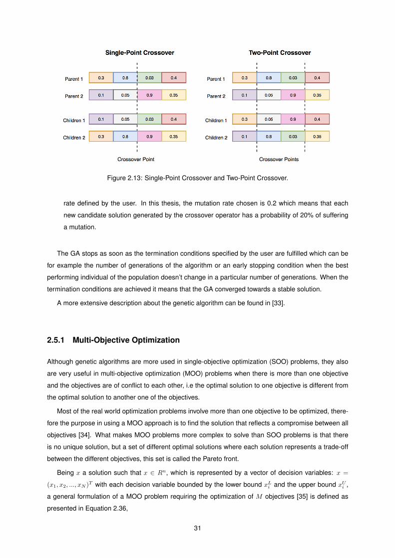
Figure 2.13: Single-Point Crossover and Two-Point Crossover.
rate defined by the user. In this thesis, the mutation rate chosen is 0.2 which means that each
new candidate solution generated by the crossover operator has a probability of 20% of suffering
a mutation.
The GA stops as soon as the termination conditions specified by the user are fulfilled which can be
for example the number of generations of the algorithm or an early stopping condition when the best
performing individual of the population doesn’t change in a particular number of generations. When the
termination conditions are achieved it means that the GA converged towards a stable solution.
A more extensive description about the genetic algorithm can be found in [33].
2.5.1 Multi-Objective Optimization
Although genetic algorithms are more used in single-objective optimization (SOO) problems, they also
are very useful in multi-objective optimization (MOO) problems when there is more than one objective
and the objectives are of conflict to each other, i.e the optimal solution to one objective is different from
the optimal solution to another one of the objectives.
Most of the real world optimization problems involve more than one objective to be optimized, there-
fore the purpose in using a MOO approach is to find the solution that reflects a compromise between all
objectives [34]. What makes MOO problems more complex to solve than SOO problems is that there
is no unique solution, but a set of different optimal solutions where each solution represents a trade-off
between the different objectives, this set is called the Pareto front.
Being x a solution such that x ∈ Rn, which is represented by a vector of decision variables: x =
(x1, x2, ..., xN )T with each decision variable bounded by the lower bound xLi and the upper bound xUi ,
a general formulation of a MOO problem requiring the optimization of M objectives [35] is defined as
presented in Equation 2.36,
31
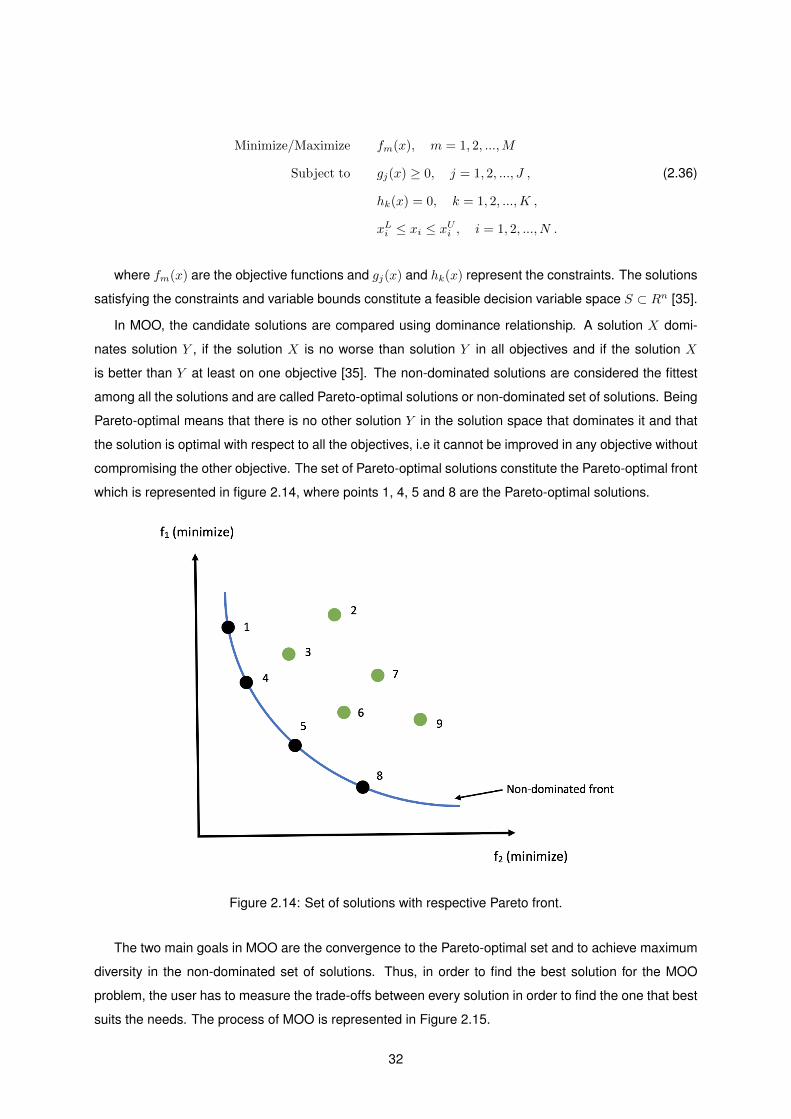
Minimize/Maximize fm(x), m = 1, 2, ...,M
Subject to gj(x) ≥ 0, j = 1, 2, ..., J , (2.36)
hk(x) = 0, k = 1, 2, ...,K ,
xLi ≤ xi ≤ xUi , i = 1, 2, ..., N .
where fm(x) are the objective functions and gj(x) and hk(x) represent the constraints. The solutions
satisfying the constraints and variable bounds constitute a feasible decision variable space S ⊂ Rn [35].
In MOO, the candidate solutions are compared using dominance relationship. A solution X domi-
nates solution Y , if the solution X is no worse than solution Y in all objectives and if the solution X
is better than Y at least on one objective [35]. The non-dominated solutions are considered the fittest
among all the solutions and are called Pareto-optimal solutions or non-dominated set of solutions. Being
Pareto-optimal means that there is no other solution Y in the solution space that dominates it and that
the solution is optimal with respect to all the objectives, i.e it cannot be improved in any objective without
compromising the other objective. The set of Pareto-optimal solutions constitute the Pareto-optimal front
which is represented in figure 2.14, where points 1, 4, 5 and 8 are the Pareto-optimal solutions.
Figure 2.14: Set of solutions with respective Pareto front.
The two main goals in MOO are the convergence to the Pareto-optimal set and to achieve maximum
diversity in the non-dominated set of solutions. Thus, in order to find the best solution for the MOO
problem, the user has to measure the trade-offs between every solution in order to find the one that best
suits the needs. The process of MOO is represented in Figure 2.15.
32
Figure 2.15: Multi-objective optimization process.
There are many multi-objective evolutionary algorithms (MOEAs), each with their own pros and cons.
Konak et. al [36] describe the most well known MOEAs identifying the the advantages and disadvan-
tages of each algorithm. In this thesis for solving the MOO problem proposed, namely the XGBoost
hyperparameters’ optimization, the Non-dominated Sorting Genetic Algorithm-II (NSGA-II) was chosen
[37]. Unlike the SOO method, the NSGA-II algorithm optimizes each objective simultaneously without
being dominated by any other solution. It is a fast MOO algorithm that uses an elitism principle and is
proven to find a much better set of solutions, as well as better convergence near the Pareto-optimal front
compared to other evolutionary algorithms, as shown by Deb et. al [37]. The NSGA-II algorithm sorts
the combination of parent and offspring populations and classifies them by fronts, having into account
the level of non-domination. Then using the crowding distance, which takes into account the density
of solutions around each solution, the mutation and crossover operators, it creates the new offspring
population that will be combined with the parent population in order to create the population for the next
generation.
The two objective functions to optimize are the accuracy of the predictions and the Sharpe ratio,
which has into account both the returns obtained and the level of risk of the trading strategies. Therefore,
the MOO-GA will search the XGBoost’s hyperparameter space for multiple combinations of hyperparam-
eters in order to find the hyperparameters that, for each financial market, allow the system to obtain the
best accuracy of the predictions and the Sharpe ratio. The chosen hyperparameters to optimize are the
ones that have a greater influence in controlling the complexity of the created models and they are: the
33
learning rate, the minimum child weight, the subsample and the maximum depth, and they are explained
in more depth in the next chapter. Therefore each one of these hyperparameters represents a gene
of the chromosome in the MOO-GA and each chromosome is a candidate solution to the given MOO
problem.
In the past years, MOO-GAs have become very popular and useful in solving optimization problems,
however there still is a lack of material regarding the optimization of models applied to the stock market.
Pimenta et. al [38] proposed a system combining technical analysis, feature selection and a MOO-
GA, namely NSGA-II, in order to maximize the financial returns while diminishing the complexity of
the model in order to avoid overfitting the data and identify suitable moments for executing buying and
selling orders. The authors tested the system in six historical time series of representative assets from
the Brazil exchange market and concluded that it consistently led to profits considerably higher than the
Buy & Hold strategy in the given period. Almeida et. al [39] proposed a system for the optimization of
stock market technical indicators parameters using the MOEA spMODE to generate Pareto fronts for
each technical indicator in order to maximize the returns, minimize the level of risk and minimize the
number of trades. The system was tested on daily IBOVESPA index data and the authors concluded
that all optimized indicators could produce excess returns when compared to the usual settings of the
parameters and that, depending on the transaction costs involved, the approach could also produce
excess returns when compared to the Buy & Hold strategy. Furthermore, Pinto et. al [40] proposed a
system combining a MOO-GA to optimize a set of trading or investment strategies. Using as inputs the
Volatility Index (VIX) and other Technical indicators, the MOO-GA searched the inputs for the best set
of indicators to use in order to find the best trade-off between returns and risk level. The system was
tested on financial indexes such as: S&P 500, NASDAQ, FTSE 100, DAX 30, and NIKKEI 225 and the
authors concluded that the achieved results outperformed both the Buy & Hold and Sell & Hold for the
period of 2006-2014. Regarding model parameters optimization, Chatelain et. al [41] proposed a MOO
method for SVM model selection using the NSGA-II algorithm in order to find the best hyperparameters
of the SVM and concluded that the MOO approach led to better results than the SOO approach, using
the Area Under the Curve (AUC) criterion.
A more extensive description about multi-objective optimization can be found in [42].
2.6 Relevant studies
Since in the past few years many studies have been developed relating the application of Machine
Learning systems to the stock market, in this section the most relevant ones that were analyzed during
the development of this thesis are presented. In Table 2.1, a summary of the most relevant studies
related with this thesis are shown.
34

35
Tabl
e2.
1:S
umm
ary
ofth
em
ostr
elev
ants
tudi
esre
late
dw
ithth
isth
esis
.
Ref
.Ye
arM
etho
dolo
gies
Per
iod
Eva
luat
ion
Met
ric
Fina
ncia
lMar
ket
Sys
tem
retu
rns
B&
Hre
turn
s
[6]
2017
AN
Nw
ithP
CA
30/1
1/20
11-
Acc
urac
yS
&P
500
Inde
xE
TF36
.1%
(Bes
tres
ult
30.8
%fo
rdim
ensi
onal
ity31
/05/
2013
(SP
Y)
w/o
trans
actio
nco
sts)
redu
ctio
n
[7]
2017
NE
ATw
ithP
CA
30/0
1/20
15-
RO
R,R
OR
/day
,S
&P
500,
Bre
nt,
18.8
9%,3
7.91
%,
15.7
1%,-
9.94
%,
ford
imen
sion
ality
13/0
4/20
17M
DP,
RR
R,
Hom
eD
epot
,CA
C40
,39
.97%
,4.6
9%,
37.6
5%,9
.82%
,re
duct
ion
MD
DS
ugar
,App
le23
.15%
,19.
73%
24.5
6%,1
9.83
%
[11]
2014
AR
IMA
with
2007
-200
9M
AD
,RM
SE
,D
euts
che
Ban
k,-
-D
WT-
base
dM
AP
EW
TIO
il,E
UR
/US
Dfo
reca
stin
gU
KPo
wer
pric
es
[21]
2016
AN
Nw
ithP
CA
2005
-201
4R
OR
,MA
PE
Nik
kei2
25,K
OS
PI,
48.2
%,7
1.1%
,8%
,11%
,an
dD
WT
deno
isin
gH
ang
Sen
g,S
iMS
CI,
34.7
%,6
8.5%
,8.
5%,7
.9%
,TA
IEX
45.4
%(B
estr
esul
ts)
7.7%
[30]
2016
XG
Boo
stlo
ng-
AUC
,RM
SE
Yaho
o,A
pple
--
term
fore
cast
[38]
2017
TAw
ithFe
atur
e02
/05/
2013
-R
OR
BB
AS
3,B
OVA
11,
54.2
0%-9
.26%
Sel
ectio
nan
dM
OO
-GA
02/0
2/20
15C
MIG
4,E
MB
R3,
(Por
tfolio
retu
rns)
(Por
tfolio
B&
H)
GG
BR
4,VA
LE5
(Bra
zilE
xcha
nge
Mar
ket)
[39]
2016
TAw
ithM
OO
-GA
2005
-201
4R
OR
IBO
VE
SPA
195.
27%
94.4
1%(B
razi
lian
stoc
kin
dex)
(Bes
tres
ult)
[40]
2015
MO
O-G
Aw
ithV
IX20
04-2
014
Ris
kE
xpos
ure,
NA
SD
AQ
,DA
X30
8.06
%(a
vera
ge)
NA
indi
cato
rR
OR
S&
P50
0,FT
SE
100
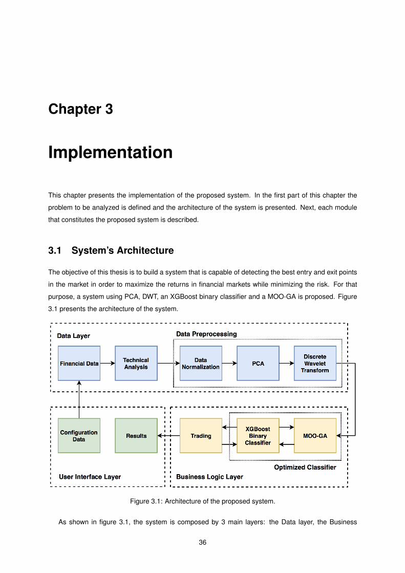
Chapter 3
Implementation
This chapter presents the implementation of the proposed system. In the first part of this chapter the
problem to be analyzed is defined and the architecture of the system is presented. Next, each module
that constitutes the proposed system is described.
3.1 System’s Architecture
The objective of this thesis is to build a system that is capable of detecting the best entry and exit points
in the market in order to maximize the returns in financial markets while minimizing the risk. For that
purpose, a system using PCA, DWT, an XGBoost binary classifier and a MOO-GA is proposed. Figure
3.1 presents the architecture of the system.
Figure 3.1: Architecture of the proposed system.
As shown in figure 3.1, the system is composed by 3 main layers: the Data layer, the Business
36

Logic layer and the User Interface layer. Using a layered architecture allows for a better organized
and structured system meaning that it’s easier to add or remove modules without interfering with the
performance of any other module.
The steps executed by the system are the following:
1. The user starts by specifying the parameters of the system like the financial data to use, the data
division and the wavelet basis, order and level of decomposition to use in the DWT;
2. From the input financial data, a set of technical indicators is obtained and a data set containing
both the raw financial data and the technical indicators is created;
3. This new data set is then fed to the data preprocessing module where it is normalized followed by
the application of the PCA technique in order to reduce its dimensionality;
4. After the dimensionality reduction is applied, the chosen wavelet basis, order and level of decom-
position are used in the DWT and noise reduction is applied to the reduced financial data set in
order to produce the input to the XGBoost module;
5. The inputs are fed to the XGBoost module and the optimization of the XGBoost binary classifier
starts by using the MOO-GA. This optimization process is done by first dividing the input set into
training, validation and test sets. The training set will be used to train the XGBoost binary clas-
sifier, the validation set will be used in order to evaluate the performance of the system and tune
the hyperparameters and after the system has its parameters tuned, the test set will be used to
evaluate the performance of the final model created by the system on unseen data;
6. The MOO-GA will optimize the XGBoost binary classifier hyperparameters and, by the means of
the validation set, the accuracy and Sharpe ratio obtained will be used in order to compare different
sets of XGBoost hyperparameters;
7. Finally, after the best set of XGBoost hyperparameters is determined, the XGBoost binary classifier
is trained using the obtained set of hyperparameters and the predictions obtained by the system
are used together with the test set in the trading module and the returns are calculated, outputting
as well the evaluation metrics’ score.
This system was implemented with the Python programming language and in the next part of this
chapter each module that constitutes the system’s architecture will be described in detail.
3.2 Target Formulation
In this thesis, the objective is to predict whether the close price for day t+1, Closet+1, will have a positive
or a negative variation with respect to the close price in the current day t, Closet. As such, a supervised
learning solution is proposed, more specifically a binary classifier. In supervised learning problems, one
has to specify the inputs to the system and the target variable to be predicted. The goal in supervised
37
learning problems is to learn the mapping function from the inputs of the system to the target variable
to be predicted and approximate the mapping function in a way that given new inputs the target variable
can be predicted correctly for this new data.
The target variable to be predicted, y, is the signal of the variation in the close price for day t+ 1 with
respect to the close price in day t and follows a binomial probability distribution y ∈ 0,1, where it takes
the value 1 if the variation in close price was positive and the value 0 if the variation in close price was
negative. This target can be mathematically defined as presented in Equation 3.1.
yt =
1 if Closet+1−ClosetCloset
≥ 0
0 if Closet+1−ClosetCloset
< 0
(3.1)
The array containing all the target variables is named Y . The input financial data set, X, is the data
set output by the data preprocessing module in which the PCA and DWT techniques are applied to the
normalized data set containing the raw financial data and the technical indicators.
3.3 Financial Data Module
The financial data module is responsible for the acquisition and storage of the daily raw financial data
of the financial market specified by the user. Depending on the source, the financial data is usually
composed by the date of the record (Date), the opening price (Open), the closing price (Close), the
highest trading price the security achieved during the trading day (High), the lowest trading price the
security achieved during the trading day (Low), the closing price (Close), the adjusted closing price
which takes into account additional factors that may change the closing price such as stock splits or new
stock offerings (AdjClose) and the amount of contracts, shares or currency traded during the trading day
(Volume).
The financial data set is provided to the system in comma-separated values (.csv) format. Figure 3.2
represents a sample of the S&P 500 index historical data taken from Yahoo Finance. The data is then
stored in a data frame using the Python library Pandas [43] which allows for an easy and fast data frame
management and handling. From the financial data the Open, High, Low, Adjusted Close and Volume
features are taken and fed to the next module of the system, the technical analysis module.
3.4 Technical Analysis Module
The technical analysis module receives as input the raw financial data from the financial data module
and applies several technical indicators to it. The main purpose of using technical indicators is that each
one provides basic information about past raw financial data in a way different from each other and thus
combining different technical indicators together helps in the detection of patterns in the financial data,
this way increasing the performance of the predictive system.
The purpose of this module is to create the data set that will serve as input to the data preprocessing
38

Figure 3.2: S&P 500 index historical data format.
module. This data set consists of the combination between the set of 26 technical indicators used, all
of them described in chapter 2, and the 5 raw financial data features, described in the previous module,
resulting in a data set with 31 features. Table 3.1 presents all the features present in the data set output
by this module. The technical indicators used in this thesis were chosen by looking at literature regarding
machine learning algorithms applied to stock market forecasting and choosing the most used ones. The
computation of the technical indicators was done using the Python library TA-Lib [44].
3.5 Data Preprocessing Module
When dealing with real-word data, there is always the chance that it is imperfect, i.e it may be noisy,
have some missing values or be inconsistent, and all these factors can lead to misleading results by the
machine learning system. Therefore, improving the overall quality of the data will consequently improve
the results. In order to do so, the raw data fed to the system must be preprocessed.
Data preprocessing is a very important step in any machine learning system that aims at making
sure that the data fed to the system is ready to be analyzed. If the data has many redundant or irrel-
evant information, or is noisy and inconsistent, during the training phase, besides fitting the model to
inadequate data, the discovery of key relationships in the data that may be crucial to the forecasting task
will be more difficult, producing misleading results. Thus, data preprocessing can significantly improve
the performance and reduce the computational costs associated to the learning phase of a machine
learning system, consequently leading to higher quality results [45].
In this thesis, the data preprocessing is done in the following way:
1. First, the data preprocessing module will read the financial data file and check for blank spaces
39

Table 3.1: List of the 31 features output to the data preprocessing module.
Technical Indicators Raw Financial Data
RSI OpenMACD, Signal Line and MACD Histogram HighPPO LowADX Adj. CloseMomentum VolumeCCIROCStochastic %D and %KWilliams %RSMA20, SMA50, SMA100EMA20, EMA50, EMA100Middle, Upper and Lower Bollinger BandsPSAROBVChaikin OscillatorMFIATR
and invalid values like for example when a number has to be an integer or a float. Once these
occurrences are identified, the lines in the financial data file that have incomplete or inconsistent
data are removed;
2. The data set obtained is then divided into training set, validation set and test set. The training set
will be used to train the model, the validation set will be used to tune the hyperparameters in order
to achieve a good generalization during the training phase and to avoid overfitting the training data
and the test set will be used as out-of-sample data in order to test the performance of the final
model in unseen data;
3. The training set will be checked for outliers, i.e extreme values that differ in a long way from the
other observations. This check for outliers is crucial for the performance of the model since the data
normalization technique applied next is sensitive to the range of values in the input data set and
having outliers would result in negative impact on the data normalization. Furthermore, having
outliers in the data can mislead the system during its training phase, resulting in less accurate
models and worst results. In order to identify and remove the outliers, besides visualizing the data
using scatterplots which allow for a better understanding of the data distribution, a data point which
is at least five times bigger than the second biggest data point or at least five times smaller than
the smallest data point is considered to be an outlier and is removed from the data set;
4. Data normalization and PCA dimensionality reduction are applied to the data set;
5. Finally the DWT is applied to the resulting data set in order to perform noise reduction.
Figure 3.3 presents the main data transformations in the data preprocessing module.
40
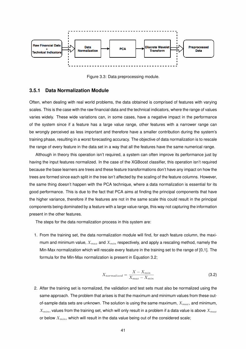
Figure 3.3: Data preprocessing module.
3.5.1 Data Normalization Module
Often, when dealing with real world problems, the data obtained is comprised of features with varying
scales. This is the case with the raw financial data and the technical indicators, where the range of values
varies widely. These wide variations can, in some cases, have a negative impact in the performance
of the system since if a feature has a large value range, other features with a narrower range can
be wrongly perceived as less important and therefore have a smaller contribution during the system’s
training phase, resulting in a worst forecasting accuracy. The objective of data normalization is to rescale
the range of every feature in the data set in a way that all the features have the same numerical range.
Although in theory this operation isn’t required, a system can often improve its performance just by
having the input features normalized. In the case of the XGBoost classifier, this operation isn’t required
because the base learners are trees and these feature transformations don’t have any impact on how the
trees are formed since each split in the tree isn’t affected by the scaling of the feature columns. However,
the same thing doesn’t happen with the PCA technique, where a data normalization is essential for its
good performance. This is due to the fact that PCA aims at finding the principal components that have
the higher variance, therefore if the features are not in the same scale this could result in the principal
components being dominated by a feature with a large value range, this way not capturing the information
present in the other features.
The steps for the data normalization process in this system are:
1. From the training set, the data normalization module will find, for each feature column, the maxi-
mum and minimum value, Xmax and Xmin respectively, and apply a rescaling method, namely the
Min-Max normalization which will rescale every feature in the training set to the range of [0,1]. The
formula for the Min-Max normalization is present in Equation 3.2;
Xnormalized =X −Xmin
Xmax −Xmin(3.2)
2. After the training set is normalized, the validation and test sets must also be normalized using the
same approach. The problem that arises is that the maximum and minimum values from these out-
of-sample data sets are unknown. The solution is using the same maximum, Xmax, and minimum,
Xmin, values from the training set, which will only result in a problem if a data value is above Xmax
or below Xmin, which will result in the data value being out of the considered scale;
41

3. The normalized training, validation and test sets are concatenated resulting in an unique normal-
ized data set that will be used as input to the PCA module.
3.5.2 PCA Module
When using a classifier to classify the data, like XGBoost, and the input data set is highly dimensional,
a problem that tends to occur is the ”Curse of dimensionality”. This problem results in a lower accuracy
achieved by machine learning classifiers due to presence of many insignificant and irrelevant features
in the input data set [46] because if more dimensions are present in the data set and the length of
the features in the training set remain the same, then overfitting will occur since the length of these
features needs to increase exponentially with relation to the number of features. In order to overcome
this problem, the use of a dimensionality reduction method is important since it reduces the dimension
of the data set which facilitates the classification process, resulting in an higher classification accuracy
while, at the same time, lowering the computational costs of machine learning systems [47]. Thus, by
reducing the dimension of the feature space, there are fewer relationships between variables to consider
and the model is less likely to overfit.
The PCA module receives the normalized input data set, containing the 26 technical indicators and
the 5 raw financial data features totaling 31 normalized features, and reduces the data set’s dimension.
These 31 features all contribute to the knowledge of the current market status by the system, each in
its own way. However, to reduce the risk of overfitting the data and to lower the computational costs of
the system, the PCA will transform the data set with 31 features in a lower dimensional one, while still
retaining most of the original data set variance. The steps for the PCA technique application used in this
system are the following:
1. The process starts again with the division of the normalized data set into training, validation and
test sets. Then, the PCA will fit its model with the normalized training set in order to generate the
parameters necessary for the application of the PCA technique. By fitting the normalized training
data, it can determine the data’s covariance matrix as well as its eigenvectors and eigenvalues
which allows for the computation of the orthogonal principal components, that represent the direc-
tions of maximum variance of the training set;
2. After the normalized training data is fitted by the PCA model, the result will be a set of principal
components, which are linear combinations of the features of the original data set. The set of
principal components produced has the same dimension of the original data set, i.e in this case
this process will result in 31 principal components, ordered by the amount of variance they explain
from the original data set, which corresponds to ordering the eigenvectors by their eigenvalue, as
already explained in section 2.2. This ordering of principal components by the amount of variance
they explain from the original data set helps in choosing which principal components to retain since
the objective is to retain the ones that explain the most variance of the original data set. Instead
of choosing the number of dimensions to reduce, an usual procedure is to choose the minimum
number of principal components that explain a given percentage of variance from the original data
42
set and retain those principal components. In this system, the number of principal components
retained is the minimum required to preserve at least 95% of the training set variance;
3. After the number of principal components selected is determined, the normalized training, val-
idation and test sets are transformed, having their data projected on the principal components
extracted from the normalized training set. The resulting data set will have a lower dimension than
the original data set due to the fact that the only principal components retained are the ones that
explain at least 95% of the original training set variance, thus removing irrelevant data samples that
were present in the original data set and only retaining the ones that better explain the relations
between the features. The training, validation and test sets are concatenated and the resulting
data set will be fed to the next module, the Wavelet module.
In Table 3.2 an example of the PCA application to the S&P500 data set (from 02/10/2006 to 11/01/2018)
is presented. The principal components of the 31 features are presented as well as the variance they
explain from the original training set. It can be noted that the first 6 principal components explain more
than 95% of the data, with a cumulative variance of 96.2287759%. Therefore instead of the original 31
features, the resulting data set will have 6 features, while still explaining most of the original training set
variance, which is a considerable reduction in dimension.
To develop the PCA module, the Scikit-learn python library [48] was used.
3.5.3 Wavelet Module
After the dimensionality reduction is applied by the PCA, the resulting data set is fed to the Wavelet
module. In this module, a noise reduction procedure is taken using the DWT.
Although in the previous module, the PCA module, the data set was already simplified having its
dimension reduced and only retaining the data that better explain the relations between the features,
obtaining a more compact representation of the original data set, some irrelevant data samples that may
have a negative impact in the training and forecasting performance of the system may still exist. While
the PCA technique removed irrelevant data points in the feature subset, the DWT technique will perform
a noise reduction in the time domain in each of the features present in the data set reduced by the PCA.
This process reduces the influence of the noise in the data set while retaining the important components
of each feature as much as possible, i.e preserving the main structure of each feature.
As already explained in section 2.3.2, the DWT performs a multilevel decomposition of the input
signal, decomposing the input signal in approximation and detail coefficients at each level of decom-
position. In this system, the parameters that will vary are the wavelet basis, the order and the level of
decomposition chosen. Due to the fact that there are many different families of wavelet basis, and each
family with many orders, in this system a set of the most common wavelet basis used in the reviewed
literature is tested, in order to find, for each financial market, the optimal wavelet basis, order and level of
decomposition that allows for a better forecasting performance. The wavelet basis tested in this system
for each financial market are:
• Haar wavelet;
43

Table 3.2: Principal components of the 31 features from the daily S&P 500 index data (from 02/10/2006to 11/01/2018).
Principal Component Variance (%) Cumulative Variance (%)
1 53.2743320 53.27433202 23.0365673 76.31089933 9.78570753 86.09660684 5.73083648 91.82744335 2.58659408 94.41403746 1.81473857 96.22877597 1.05158137 97.28035738 0.66593963 97.94629699 0.59252985 98.5388268
10 0.41654443 98.955371211 0.33378579 99.289157012 0.22345921 99.512616213 0.18714084 99.699757114 0.09112768 99.790884815 0.06112955 99.852014316 0.04298150 99.894995817 0.02935113 99.924346918 0.02464489 99.948991819 0.02307677 99.972068620 0.00897104 99.981039621 0.00707116 99.988110822 0.00476174 99.992872523 0.00358779 99.996460324 0.00170643 99.998166725 0.00098628 99.999153026 0.00047742 99.999630427 0.00029730 99.999927728 0.00004518 99.999972929 0.00002707 100.000000030 1.4209E-32 100.000000031 9.5220E-33 100.0000000
• Daubechies wavelet of order: 3, 6, 9, 15 and 20;
• Symlet wavelet of order: 3, 6, 9, 15 and 20.
Although with more decomposition levels more noise can be removed and therefore resulting in a
better representation of the trend of each feature, this could also result in removing fluctuations that
carry market characteristics. Therefore in this system, the levels of decomposition tested are 2, 5 and 7
(7 is the maximum decomposition level allowed by the decomposition algorithm in this system), in order
to find the optimal denoising level of decomposition for each financial market.
Since each financial market has its own characteristics, the objective is to find, for each financial
market, the optimal combination of wavelet basis and level of decomposition in order to obtain the better
44

forecasting performance.
The steps for the DWT technique application used in this system are the following:
1. The process starts by specifying the wavelet basis, order and the level of decomposition that will be
used. Then, for each of the training set’s features, the DWT performs the multilevel decomposition
which will result in one set of approximation coefficient and j sets of detail coefficients, with j
being the chosen decomposition level, as explained in section 2.3.2. Since the DWT is a parametric
process, i.e for the same input signal but varying its length, a whole new set of different coefficients
is obtained since it makes assumptions on the distribution of the parameters of the signal, the
set of coefficients for the training set needs to be calculated separately from the out-of-sample
validation and test sets. This is due to the fact that if the whole feature’s data points were used,
the coefficients obtained would be having future information into account since the coefficients
obtained in one time instant would be influenced by the distribution of the data points succeeding
it. Therefore, in order to calculate the approximation and detail coefficients for both the validation
and test sets, one data point at a time is added to the training set, the coefficients for the new
signal are calculated and the coefficients corresponding to the data point added are saved. This
procedure is performed until all the points in the validation and test sets have their respective
coefficients calculated.
2. After the coefficients for both training, validation and test sets are obtained, the BayesShrink and
soft thresholding approach is applied to the set of detail coefficients in each decomposition level,
resulting in a set of detail coefficients containing only the detail coefficients that capture the im-
portant features of the original signal and discarding the irrelevant ones. Using suitable shrinkage
and thresholding methods on the detail coefficients allow for a noise reduction while preserving
the important characteristics of each feature;
3. After the thresholding method is applied to all detail coefficients in each decomposition level, the
set of approximation coefficients is used together with the obtained set of thresholded detail coef-
ficients in the signal reconstruction phase. The reconstruction is made by performing the inverse
DWT. By using the set of approximation coefficients and the set of thresholded detail coefficients,
the result is a denoised version of each of the original data set’s features, where irrelevant data
points that could have a negative impact on the system’s performance have their importance low-
ered, achieving the purpose of the noise reduction method which is to retain the energy of the
original signal while discarding the energy of the noise present in the signal.
After the application of the DWT, the data set is ready to be fed to the next module, the XGBoost
module. Having an input data set with both the dimensionality and noise reduced will allow for a better
generalization and learning by the XGBoost binary classifier applied in the next module.
The PyWavelets [49] and scikit-image [50] python libraries were used to develop the DWT module in
this system.
45

3.6 XGBoost Module
Now that the input set, as well as the target variable array, Y , to be predicted are defined, the XGBoost
module is ready to be used. This module receives the preprocessed data set from the data prepro-
cessing module, as well as the target variable array Y , performs a binary classification based on the
forecasting of the input data set and outputs the trading signal to the training module.
This module is the core of the system, it’s where the patterns in the input data set are discovered
and the XGBoost binary classifier has its performance improved by the means of an hyperparameter’s
optimization using the MOO-GA presented in the next section, thus capable of a better generalization
of the training set data than simply using the default values for the hyperparameters. After the XGBoost
binary classifier has its parameters tuned by the MOO-GA, this same set of hyperparameters, consid-
ered the most fit among all the tested sets of hyperparameters, is used to train the final XGBoost binary
classifier which will test the model with the out-of-sample test set in order to check if the solution found
has a good generalization capacity or not.
This module is divided in two parts, the XGBoost binary classifier and the hyperparameter’s multi-
objective optimization by the means of a MOO-GA, explained in the next sections.
3.6.1 XGBoost Binary Classifier Module
The XGBoost binary classifier is the responsible for the classification process of the system. Given the
financial data set matrix, X, output by the data preprocessing module and the target variable array, Y ,
to be classified, a model like the one presented in Figure 3.4 can be constructed. An example of these
two inputs is presented in Figure 3.5. The way the XGBoost binary classifier is trained is explained in
section 2.4.
Figure 3.4: XGBoost binary classifier model.
The output of the classifier, yt, is the predicted value given the current observation, xt, corresponding
to the actual day, t. The variable yt is in the range [0,1] and the set of all yt corresponds to the predicted
trading signal which indicates if the system should take a Long or Short position in the next trading day.
Before the XGBoost binary classifier algorithm starts, a set of parameters must be chosen. The
parameters which define a Machine Learning system architecture are referred to as hyperparameters.
The hyperparameters in the XGBoost are divided into three types:
• General hyperparameters, related to the overall functioning of the algorithm, i.e the type of
booster to use and additional features to aid in the computational task. In this system the type
46

Figure 3.5: Inputs to the XGBoost binary classifier.
of booster used is the gbtree which uses tree based models;
• Booster hyperparameters, related to the chosen type of booster. For the gbtree booster this hy-
perparameters are for example the learning rate, the maximum depth of the tree or the subsample
fraction of the training instance;
• Learning task hyperparameters, that guide the algorithm during the learning phase by specify-
ing the learning task and the corresponding learning objective. These hyperparameters are for
example the optimization objective and the loss function. In this system the optimization objective
is the binary:logistic method which is logistic regression for binary classification and returns the
predicted probability of y belonging to a given class. The classes chosen are the ones explained
in 3.2, if p(yt) ≥ 0.5 then yt is classified as belonging to class 1 and conversely, if p(yt) < 0.5 then
yt is classified as belonging to class 0;
The loss function chosen is the Area Under the Curve (AUC). The loss value implies how well a
certain model behaves after each iteration of optimization. Ideally, the objective is the loss value
reduction after each, or several, iterations. The ROC curve is created by plotting the true positive
rate against the false positive rate at varied threshold values.
In Machine Learning one aspect to always have into account when developing a system is the bias-
variance trade-off. Bias can be seen as the simplifying assumptions made by a model in order to make
the target function easier to learn and variance is how much the estimate of the target function changes if
different training data was used. A model with a low bias will suggest less assumptions about the shape
of the target function, conversely a model with an high bias suggests more assumptions about the shape
of the target function. When the training data changes, a model with a low variance will suggest small
changes to the estimate of the target function, while a model with an high variance will suggest large
changes to the estimate of the target function. The main objective in any supervised machine learning
47

algorithm is to achieve low bias and low variance since an high bias model will generalize well but will
end up not fitting the data properly and although an high variance model will fit the training data well,
it will in fact fit the data too well that it makes generalization a problem. Most of the hyperparameters
in XGBoost are about this bias and variance trade-off, thus the best model should be able to find the
balance between complexity and predictive power.
Because every time series has its own characteristics, for every time series analyzed there is a
different set of optimal hyperparameters, i.e hyperparameters that allow for the model to have a good
generalization capacity and therefore achieve good results in out-of-sample data. Therefore, in order to
achieve the best results in each of the analyzed financial market, the optimal set of hyperparameters
has to be found. In order to do so, the MOO-GA approach is used, as presented in the next section.
After the hyperparameters are tuned by the MOO-GA, the XGBoost classifier algorithm is ready to
begin. Figure 3.6 presents the architecture of the XGBoost classifier.
Figure 3.6: XGBoost classifier architecture.
The preprocessed data output by the data preprocessing module is fed to the XGBoost binary clas-
sifier, as well as the target variable array, Y , to be predicted and both are divided into training, validation
and test sets. With both the data sets and the XGBoost hyperparameters defined, the training phase
starts. During the training phase, the XGBoost binary classifier receives the training data set (the finan-
cial data set and the target variable to be predicted) as input and uses this training set to produce an
inferred function (f ) that can be used for mapping new out-of-sample data (X) to a target output variable
(Y ), as presented in Equation 3.3.
Y = f(X) (3.3)
The number of boosting rounds chosen for each model is 100, which corresponds to the number of
trees constructed. This value was the one considered optimal for this system and was left at 100 since
optimizing it would sometimes result in too complex models that would not generalize well to unseen
data and therefore would make poor predictions. As the number of boosting rounds increases, the
complexity of the model also tends to increase, therefore a number of boosting rounds higher than 100
in this system often lead to overfitting the training data.
48
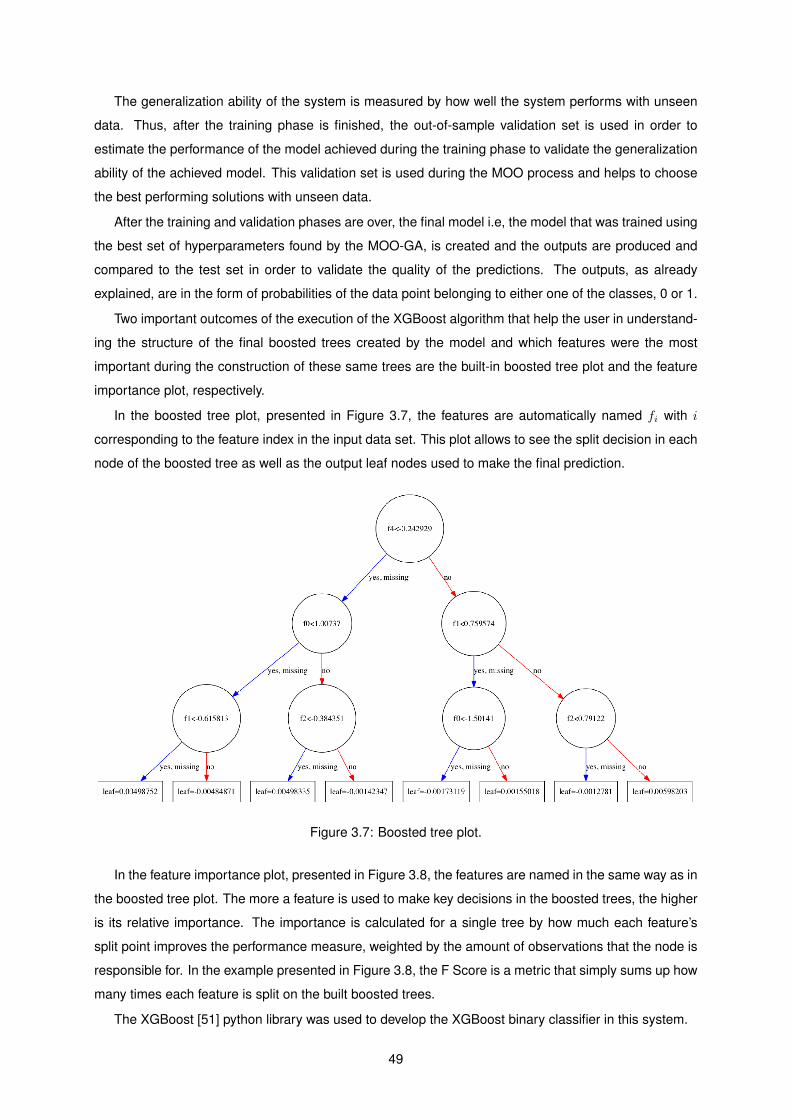
The generalization ability of the system is measured by how well the system performs with unseen
data. Thus, after the training phase is finished, the out-of-sample validation set is used in order to
estimate the performance of the model achieved during the training phase to validate the generalization
ability of the achieved model. This validation set is used during the MOO process and helps to choose
the best performing solutions with unseen data.
After the training and validation phases are over, the final model i.e, the model that was trained using
the best set of hyperparameters found by the MOO-GA, is created and the outputs are produced and
compared to the test set in order to validate the quality of the predictions. The outputs, as already
explained, are in the form of probabilities of the data point belonging to either one of the classes, 0 or 1.
Two important outcomes of the execution of the XGBoost algorithm that help the user in understand-
ing the structure of the final boosted trees created by the model and which features were the most
important during the construction of these same trees are the built-in boosted tree plot and the feature
importance plot, respectively.
In the boosted tree plot, presented in Figure 3.7, the features are automatically named fi with i
corresponding to the feature index in the input data set. This plot allows to see the split decision in each
node of the boosted tree as well as the output leaf nodes used to make the final prediction.
Figure 3.7: Boosted tree plot.
In the feature importance plot, presented in Figure 3.8, the features are named in the same way as in
the boosted tree plot. The more a feature is used to make key decisions in the boosted trees, the higher
is its relative importance. The importance is calculated for a single tree by how much each feature’s
split point improves the performance measure, weighted by the amount of observations that the node is
responsible for. In the example presented in Figure 3.8, the F Score is a metric that simply sums up how
many times each feature is split on the built boosted trees.
The XGBoost [51] python library was used to develop the XGBoost binary classifier in this system.
49
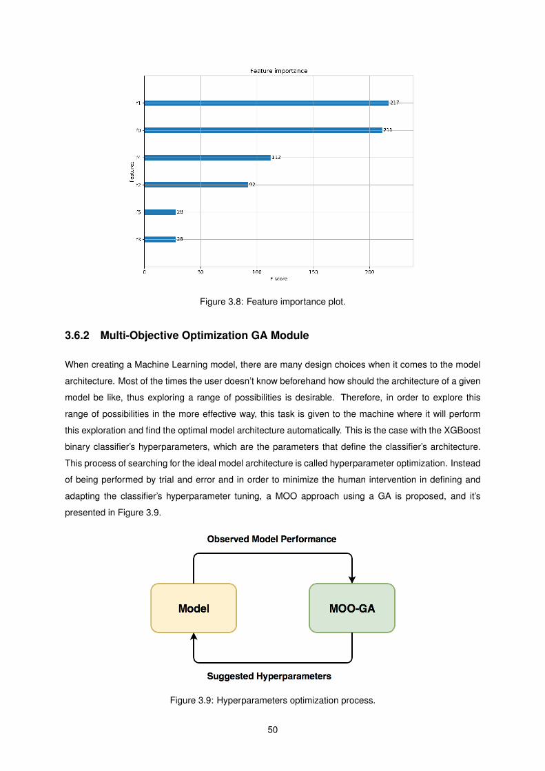
Figure 3.8: Feature importance plot.
3.6.2 Multi-Objective Optimization GA Module
When creating a Machine Learning model, there are many design choices when it comes to the model
architecture. Most of the times the user doesn’t know beforehand how should the architecture of a given
model be like, thus exploring a range of possibilities is desirable. Therefore, in order to explore this
range of possibilities in the more effective way, this task is given to the machine where it will perform
this exploration and find the optimal model architecture automatically. This is the case with the XGBoost
binary classifier’s hyperparameters, which are the parameters that define the classifier’s architecture.
This process of searching for the ideal model architecture is called hyperparameter optimization. Instead
of being performed by trial and error and in order to minimize the human intervention in defining and
adapting the classifier’s hyperparameter tuning, a MOO approach using a GA is proposed, and it’s
presented in Figure 3.9.
Figure 3.9: Hyperparameters optimization process.
50
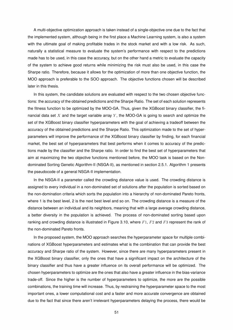
A multi-objective optimization approach is taken instead of a single-objective one due to the fact that
the implemented system, although being in the first place a Machine Learning system, is also a system
with the ultimate goal of making profitable trades in the stock market and with a low risk. As such,
naturally a statistical measure to evaluate the system’s performance with respect to the predictions
made has to be used, in this case the accuracy, but on the other hand a metric to evaluate the capacity
of the system to achieve good returns while minimizing the risk must also be used, in this case the
Sharpe ratio. Therefore, because it allows for the optimization of more than one objective function, the
MOO approach is preferable to the SOO approach. The objective functions chosen will be described
later in this thesis.
In this system, the candidate solutions are evaluated with respect to the two chosen objective func-
tions: the accuracy of the obtained predictions and the Sharpe Ratio. The set of each solution represents
the fitness function to be optimized by the MOO-GA. Thus, given the XGBoost binary classifier, the fi-
nancial data set X and the target variable array Y , the MOO-GA is going to search and optimize the
set of the XGBoost binary classifier hyperparameters with the goal of achieving a tradeoff between the
accuracy of the obtained predictions and the Sharpe Ratio. This optimization made to the set of hyper-
parameters will improve the performance of the XGBoost binary classifier by finding, for each financial
market, the best set of hyperparameters that best performs when it comes to accuracy of the predic-
tions made by the classifier and the Sharpe ratio. In order to find the best set of hyperparameters that
aim at maximizing the two objective functions mentioned before, the MOO task is based on the Non-
dominated Sorting Genetic Algorithm-II (NSGA-II), as mentioned in section 2.5.1. Algorithm 1 presents
the pseudocode of a general NSGA-II implementation.
In the NSGA-II a parameter called the crowding distance value is used. The crowding distance is
assigned to every individual in a non-dominated set of solutions after the population is sorted based on
the non-domination criteria which sorts the population into a hierarchy of non-dominated Pareto fronts,
where 1 is the best level, 2 is the next best level and so on. The crowding distance is a measure of the
distance between an individual and its neighbors, meaning that with a large average crowding distance,
a better diversity in the population is achieved. The process of non-dominated sorting based upon
ranking and crowding distance is illustrated in Figure 3.10, where F1, F2 and F3 represent the rank of
the non-dominated Pareto fronts.
In the proposed system, the MOO approach searches the hyperparameter space for multiple combi-
nations of XGBoost hyperparameters and estimates what is the combination that can provide the best
accuracy and Sharpe ratio of the system. However, since there are many hyperparameters present in
the XGBoost binary classifier, only the ones that have a significant impact on the architecture of the
binary classifier and thus have a greater influence on its overall performance will be optimized. The
chosen hyperparameters to optimize are the ones that also have a greater influence in the bias-variance
trade-off. Since the higher is the number of hyperparameters to optimize, the more are the possible
combinations, the training time will increase. Thus, by restraining the hyperparameter space to the most
important ones, a lower computational cost and a faster and more accurate convergence are obtained
due to the fact that since there aren’t irrelevant hyperparameters delaying the process, there would be
51
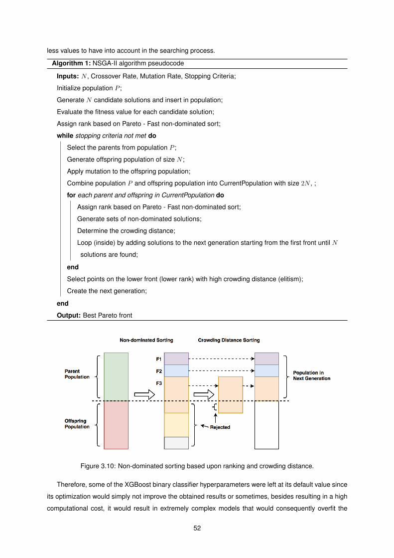
less values to have into account in the searching process.
Algorithm 1: NSGA-II algorithm pseudocode
Inputs: N , Crossover Rate, Mutation Rate, Stopping Criteria;
Initialize population P ;
Generate N candidate solutions and insert in population;
Evaluate the fitness value for each candidate solution;
Assign rank based on Pareto - Fast non-dominated sort;
while stopping criteria not met do
Select the parents from population P ;
Generate offspring population of size N ;
Apply mutation to the offspring population;
Combine population P and offspring population into CurrentPopulation with size 2N , ;
for each parent and offspring in CurrentPopulation do
Assign rank based on Pareto - Fast non-dominated sort;
Generate sets of non-dominated solutions;
Determine the crowding distance;
Loop (inside) by adding solutions to the next generation starting from the first front until N
solutions are found;
end
Select points on the lower front (lower rank) with high crowding distance (elitism);
Create the next generation;
end
Output: Best Pareto front
Figure 3.10: Non-dominated sorting based upon ranking and crowding distance.
Therefore, some of the XGBoost binary classifier hyperparameters were left at its default value since
its optimization would simply not improve the obtained results or sometimes, besides resulting in a high
computational cost, it would result in extremely complex models that would consequently overfit the
52
training data and make poor predictions.
The XGBoost binary classifier hyperparameters that are optimized are:
• Learning rate- Defines how quickly the model learns. An higher learning rate means that the
model will learn faster and will make rough distinctions between the classes. A lower learning rate
means that the model will have a slower and more careful learning. The values are in the range
]0, 1];
• Maximum tree depth - The maximum allowable depth for each decision tree. The number of
nodes in each tree increases by 2depth, thus by increasing the maximum depth of each tree, the
complexity also increases. Therefore one way to avoid getting very complex models that could
result in overfitting the training data is reducing the maximum tree depth. The values are in the
range [0,∞[;
• Minimum child weight - The minimum sum of instance weight (hessian) that is needed in a child.
If the tree partition step results in a leaf node with the sum of instance weight less than minimum
child weight, then the building process gives up further partitioning. The values are in the range
[0,∞[;
• Subsample - The subsample ratio of the training instance. For example, setting it to 0.5 means
that XGBoost will randomly collect half of the training data instances to grow the trees, which helps
in preventing overfitting the training data. The goal of subsampling is to reduce the variance of the
model. The values are in the range ]0, 1].
These optimized hyperparameters constitute the set of Booster hyperparameters used in the system,
presented before in section 3.6.1. Each one of the four hyperparameters presented before constitute a
gene of the chromosome in the MOO-GA.
Before the MOO-GA starts, in order to explore various model architectures that come up with the dif-
ferent hyperparameter sets obtained, a way to evaluate each hyperparameter set obtained is to evaluate
the resulting model’s ability to generalize to unseen data. However, this process can’t be done using the
test set since the system would end up fitting the model architecture to the test set which would result
in the loss of the ability to forecast unseen data. In order to mitigate this, the validation set is used since
it allows the evaluation of the model on a different, unseen, data set than the one it was trained with
and select the best performing model architecture with unseen data. The test set is used for the final
evaluation of the model’s generalization ability at the end of the model development.
The MOO-GA starts with the creation, in each generation, of a chromosome population with size N
that will have their fitness evaluated. After the population is created, each chromosome will be used
as the hyperparameter set of an XGBoost binary classifier that will be used to make predictions on the
validation set. The XGBoost binary classifier is trained using both the financial data set X and the target
variable array Y as inputs and after the training phase is finished the predictions in the validation set
are made. After the predictions are made, the accuracy of the predictions is calculated as well as the
obtained Sharpe ratio, and these two obtained values constitute the fitness values of the chromosome.
53
After all the individuals have their fitness calculated, they are sorted based on the non-domination cri-
teria with an assigned fitness (rank) equal to its non-domination level. The parents are selected from
the population using a binary tournament selection based on the rank and crowding distance. To the
individuals that were selected, the crossover and mutation operators are applied in order to generate
the offspring population. This new offspring population is combined with the parent population and the
resulting population, with size 2N , is sorted again based on non-domination. After this process, only
the best N individuals are selected, where N is the population size, and these individuals constitute the
next population. This cycle is repeated until the termination conditions are fulfilled. The NSGA-II is also
an elitist MOO-GA, therefore it keeps record of the best solutions from the previous population.
Elitism
Sometimes, after crossover and mutation are applied, the fittest individuals of a population can be lost,
resulting in an offspring population that is weaker than the parent population which is a problem when
optimizing an objective function. Often the evolutionary algorithm re-discovers these lost individuals in
a subsequent generation, but with no guarantees. Thus, in order to guarantee that the fittest individuals
aren’t discarded during the evolutionary process, a feature known as elitism is used. Elitism involves
copying a small portion of the fittest individuals of a population unchanged to the next generation, in
each generation preventing that the genes of the fittest individuals are changed by the crossover and
mutation operators which could result in decreasing the highest fitness value from one generation to
the following one. These candidates solutions that remain unchanged through the use of elitism remain
eligible for the selection process as parents.
In the NSGA-II when the offspring population is combined with the current generation population and
the selection process is performed in order to determine the individuals of the next generation, since the
previous and current best individuals are always added to the population, elitism is ensured.
Hypermutation
First introduced by Cobb [52], hypermutation is a method for reintroducing diversity into the population
in an evolutionary algorithm. The goal of hypermutation is to change the mutation rate when the trigger
is fired, based on the state of the searching process. In this system the mutation rate is adjusted during
the evolutionary process in order to help the algorithm jump out of a local optimum, i.e when it considers
that it is very close to the maximum fitness and starts to stagnate. Therefore, when the hypermutation
trigger is fired, the overall mutation rate increases from its original value of 0.2, and this happens when:
• The obtained set of non-dominated solutions doesn’t change in 4 generations, increasing the over-
all mutation rate by 0.1;
• The obtained set of non-dominated solutions doesn’t change in 6 generations, increasing the over-
all mutation rate by 0.15;
54

• The obtained set of non-dominated solutions still hasn’t changed in 8 generations, again increasing
the overall mutation rate by 0.15.
• When the set of non-dominated solutions changes then the overall mutation rate goes back to its
original value of 0.2.
Fitness Functions
The fitness function is a function that estimates the success of the candidate solution (chromosome) in
solving the desired problem, i.e it determines how fit the candidate solution is. By determining the fitness
of each candidate solution, it allows to make a clear distinction between the best and worst performing
solutions. The goal of this separation between the best and worst performing solutions is that later on
the execution of the algorithm, the best performing solutions will have a higher chance of being picked
to form the next generation.
Therefore, given its importance in evaluating all the candidate solutions, the fitness function should
be clearly defined i.e, it should be clear how the fitness scores are being computed and should give
intuitive results i.e, an increase in the fitness value should be followed by an increase in the solution’s
performance, this way supporting the evolvability of the system. In order to negatively impact the overall
performance of the system, the fitness function should be implemented efficiently since the fitness value
is calculated many times over the course of the algorithm’s execution.
In this system a MOO approach is taken and as the name implies more than one objective function is
optimized with the goal of finding the best combination of hyperparameters that maximizes the objective
functions. In this case, the fitness functions and the objective functions are the same, as the objective is
to maximize the objective functions.
When there are more than one fitness values to be optimized together, conflicts of interest may arise
between the objective functions since the optimal solution for one of the objectives will not necessary
be the optimal solution for the other objectives. Therefore, each one of the obtained solutions will
produce different trade-offs between the different objectives and the goal is to find the one that reflects
a compromise between all the objectives.
Since in the first place, the developed system’s predictor is a binary classifier, the accuracy of the
XGBoost binary classifier in making predictions must be taken into account in the MOO process and it
is one of the fitness functions. The accuracy of the model is determined after the model parameters are
learned and fixed and no learning is taking place. Then the out-of-sample set is fed to the model and
the number of mistakes are recorded, after comparing them to the true targets and the accuracy of the
predictions made is calculated, using the expression in Equation 3.4.
Accuracy =Number of Correct Predictions
Number of Predictions∗ 100 (3.4)
However, the goal of the system is also to maximize the returns obtained in the market while mini-
mizing the risk associated to the trades. Thus, a fitness function capable of measuring the performance
of the system in making profitable trades while minimizing the risk is also used. This fitness function is
55
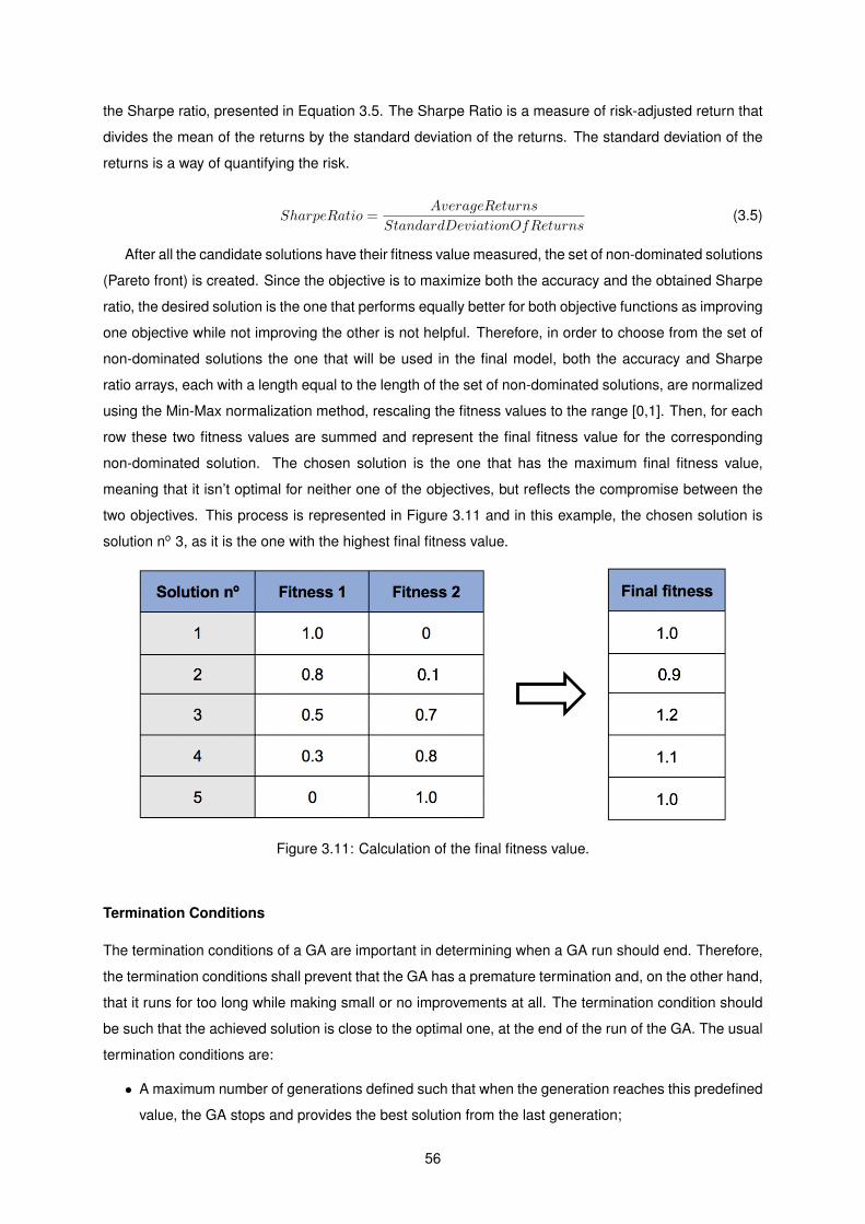
the Sharpe ratio, presented in Equation 3.5. The Sharpe Ratio is a measure of risk-adjusted return that
divides the mean of the returns by the standard deviation of the returns. The standard deviation of the
returns is a way of quantifying the risk.
SharpeRatio =AverageReturns
StandardDeviationOfReturns(3.5)
After all the candidate solutions have their fitness value measured, the set of non-dominated solutions
(Pareto front) is created. Since the objective is to maximize both the accuracy and the obtained Sharpe
ratio, the desired solution is the one that performs equally better for both objective functions as improving
one objective while not improving the other is not helpful. Therefore, in order to choose from the set of
non-dominated solutions the one that will be used in the final model, both the accuracy and Sharpe
ratio arrays, each with a length equal to the length of the set of non-dominated solutions, are normalized
using the Min-Max normalization method, rescaling the fitness values to the range [0,1]. Then, for each
row these two fitness values are summed and represent the final fitness value for the corresponding
non-dominated solution. The chosen solution is the one that has the maximum final fitness value,
meaning that it isn’t optimal for neither one of the objectives, but reflects the compromise between the
two objectives. This process is represented in Figure 3.11 and in this example, the chosen solution is
solution no 3, as it is the one with the highest final fitness value.
Figure 3.11: Calculation of the final fitness value.
Termination Conditions
The termination conditions of a GA are important in determining when a GA run should end. Therefore,
the termination conditions shall prevent that the GA has a premature termination and, on the other hand,
that it runs for too long while making small or no improvements at all. The termination condition should
be such that the achieved solution is close to the optimal one, at the end of the run of the GA. The usual
termination conditions are:
• A maximum number of generations defined such that when the generation reaches this predefined
value, the GA stops and provides the best solution from the last generation;
56

• The GA proceeds until the highest fitness score found during the evolution process doesn’t improve
over a given predefined number of generations, meaning that the GA may have converged.
As such, these usual termination conditions will be used in this system. One key point to have into
account when using a GA as an optimization algorithm is that there is no guarantee that it will find an
optimal solution in a finite time. Therefore, the bound of good enough performance should be chosen
carefully since if it is too low the system’s performance may be limited, but if it is too high it may never
achieve a solution that reaches the chosen bound. The two termination conditions chosen for the MOO-
GA in this system are:
• The algorithm reaches 100 generations;
• The set of non-dominated solutions doesn’t change for 10 generations.
With these termination conditions, the algorithm doesn’t have great computational costs by being
bounded by 100 generations while at the same time avoiding an excess of computations that could
result in overfit by terminating the algorithm if the set of non-dominated solutions doesn’t change for
10 generations. When one of the termination conditions is achieved, the MOO-GA stops its execution
and outputs the solution with the highest fitness score that will be used to train the final XGBoost binary
classifier which will output the predictions that constitute the trading signal, used in the next module.
The DEAP [53] python library was used to develop the MOO-GA module in this system.
3.7 Trading Module
The trading module is the module responsible for simulating trades in real financial markets. It receives
as input the trading signal output by the XGBoost module and financial data and simulates the market
orders in a financial market.
The trading module starts with 100000 dollars as initial capital for investment and will execute the
market orders according to the trading signal. In order to execute the trades, this simulator was designed
as a state machine with the states Long, Short and Hold. In financial markets, a Long position is the
buying of a security with the expectation that its price will have a positive variation, therefore rising in
value. Conversely, the Short position is the inverse of the Long position, and is the sale of a security
that is not owned by the seller, therefore with the expectation that its price will have a negative variation.
The system will go to the Hold state if the current position is the same as the previous one, this way
holding the Long position or holding the Short position. In each transaction made, there are associated
transaction costs that depend on the financial market where the transactions are being made. For each
financial market tested, the associated transaction costs are present in the next chapter.
Given the trading signal, a state machine is executed according to the market orders present in the
trading signal. The state machine diagram is presented in Figure 3.13 with its three states and the
actions that can be taken in each state.
57
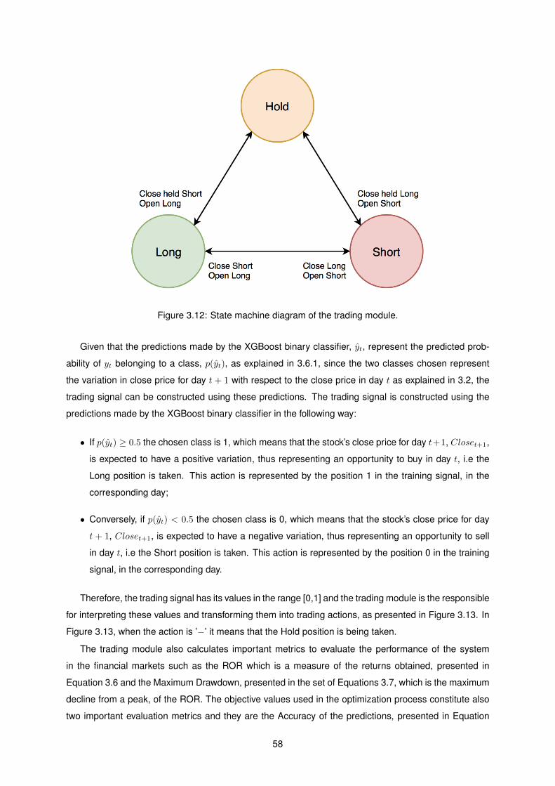
Figure 3.12: State machine diagram of the trading module.
Given that the predictions made by the XGBoost binary classifier, yt, represent the predicted prob-
ability of yt belonging to a class, p(yt), as explained in 3.6.1, since the two classes chosen represent
the variation in close price for day t + 1 with respect to the close price in day t as explained in 3.2, the
trading signal can be constructed using these predictions. The trading signal is constructed using the
predictions made by the XGBoost binary classifier in the following way:
• If p(yt) ≥ 0.5 the chosen class is 1, which means that the stock’s close price for day t+1, Closet+1,
is expected to have a positive variation, thus representing an opportunity to buy in day t, i.e the
Long position is taken. This action is represented by the position 1 in the training signal, in the
corresponding day;
• Conversely, if p(yt) < 0.5 the chosen class is 0, which means that the stock’s close price for day
t + 1, Closet+1, is expected to have a negative variation, thus representing an opportunity to sell
in day t, i.e the Short position is taken. This action is represented by the position 0 in the training
signal, in the corresponding day.
Therefore, the trading signal has its values in the range [0,1] and the trading module is the responsible
for interpreting these values and transforming them into trading actions, as presented in Figure 3.13. In
Figure 3.13, when the action is ’−’ it means that the Hold position is being taken.
The trading module also calculates important metrics to evaluate the performance of the system
in the financial markets such as the ROR which is a measure of the returns obtained, presented in
Equation 3.6 and the Maximum Drawdown, presented in the set of Equations 3.7, which is the maximum
decline from a peak, of the ROR. The objective values used in the optimization process constitute also
two important evaluation metrics and they are the Accuracy of the predictions, presented in Equation
58

Figure 3.13: Trading module execution example with S&P 500 data.
3.4 and the Sharpe Ratio, presented in Equation 3.5. The number of transactions is also registered in
order to understand how was the system’s behaviour in each financial market.
ROR =FinalCapital − InitialCapital
InitialCapital∗ 100 (3.6)
DrawDownt = Maxi∈(Start Date,t)(RORi −RORt) , (3.7a)
MaxDrawDown = Maxt∈(Start Date,End Date)(DrawDownt) , (3.7b)
The results obtained by the Trading module for the different evaluation metrics are used in the next
chapter for the analysis of the case studies where the performance of different systems is evaluated.
59

Chapter 4
Results
In this chapter, the results obtained using the proposed system described in the previous chapter are
presented. First, the different financial markets in which the system was tested and the evaluation
metrics used to test the performance of the system are presented. Next, the results of the system
using either the PCA or DWT techniques when applied to the financial data are presented in order to
analyze the importance of these components in the system’s performance when applied separately.
Then, the results of the system when using both PCA and DWT are presented and analyzed. Finally, a
performance comparison between the system proposed in this thesis and a similar one is provided.
The experiments were conducted using a MacBook Pro laptop, with a 2.30 GHz dual-core i5 Intel
processor and 8GB of RAM, running macOS High-Sierra operating system, resulting in an execution
time for each generation of the MOO-GA, which is the bottleneck of the system, of approximately 30
seconds. Given that in each run of the MOO-GA, it may or may not converge and therefore resulting
in many different solutions, each experiment was made using 10 different runs in order to obtain an
average of the system’s performance and the results presented in the next sections are this average of
the system’s performance.
In this system the same set of hyperparameters was used both in the PCA, XGBoost binary classifier
(apart from the ones being optimized) and in the MOO-GA, regardless of the financial data being ana-
lyzed, in order to demonstrate that the proposed system is robust and capable of working with different
financial markets. The only varying parameters between financial markets are the ones used in the
DWT since the objective is to find both the best wavelet basis, order and level of decomposition for each
analyzed financial market and the set of XGBoost hyperparameters that are optimized by the MOO-GA.
Since in the experiments presented in the next sections, presenting the return plots for each analyzed
financial market would be too extensive, only the return plots for two financial market are presented
with the exception of the Case Study III where the return plots for every analyzed financial market are
presented. However, more detailed results for every analyzed financial market are present in the tables
that come along with the plots of the returns.
60
4.1 Financial Data
In order to train, validate and test the proposed system, financial data from five different financial markets
is used. This financial data consists of the daily prices (Open, High, Low, Close and Adjusted Close) and
Volume over the period of 25/02/2003 to 10/01/2018. From this data, 60% is used to train the system
in order to generate all the predictive models, 20% to validate the models obtained and 20% to test the
final model obtained after all the training has been done. Thus, the system is trained from 25/02/2003 to
29/11/2011 (2209 trading days), validated from 30/11/2011 to 19/12/2014 (769 trading days) and tested
from 22/12/2014 to 10/01/2018 (769 trading days).
In order to test the robustness of the proposed system to different financial markets, each with their
own behaviour and this way ensuring diversity in the experiments made, the experiments are performed
in the following financial markets:
• Brent Crude futures contract;
• Corn futures contract;
• Exxon Mobil Corporation (XOM ticker symbol) stocks;
• Home Depot Inc. (HD ticker symbol) stocks;
• S&P 500 index (United States of America Stock Market Index).
The S&P 500, Exxon Mobil Corporation and Home Depot Inc. financial data were acquired from
Yahoo Finance and the Brent Crude futures and Corn futures financial data were acquired from Quandl.
In each transaction made in a financial market, a fee applies and it is called transaction cost. The
transaction costs are included in the trading module and, for each financial market analyzed, they are
the following:
• Brent Crude futures contract and Corn futures contract: 0.1% of the transaction value;
• Exxon Mobil Corporation and Home Depot Inc. stocks: 0.005 USD per stock transacted;
• S&P 500 index: 1 USD per stock transacted.
4.2 Evaluation metrics
As already mentioned in section 3.6.2, the goal of the system is to maximize the returns obtained in
the market while minimizing the risk associated to the trades made. However, since in the developed
system the predictor used is a binary classifier, the accuracy of the predictions made by the final model
obtained by the system must be also taken into account.
Although these evaluation metrics were already presented in the previous chapter, for the reader’s
convenience they are presented again. The metrics used in order to evaluate the system’s performance
in the financial markets are:
61
• The Rate of Return (ROR), presented in Equation 4.1. The ROR allows to evaluate the returns
obtained by the system in a financial market;
ROR =FinalCapital − InitialCapital
InitialCapital∗ 100 (4.1)
• The Maximum DrawDown (MDD), presented in the set of Equations 4.2. The MDD is used in order
to measure the risk associated to investments. Low values of MDD are desirable which means
that the risk is low and therefore the possible losses will also be low;
DrawDownt = Maxi∈(Start Date,t)(RORi −RORt) , (4.2a)
MaxDrawDown = Maxt∈(Start Date,End Date)(DrawDownt) (4.2b)
• The accuracy of the predictions made by the XGBoost binary classifier, presented in Equation 4.3.
The accuracy is the number of correct predictions made divided by the total number of predictions
made, multiplied by 100 to turn it into a percentage and is useful to understand how well the
binary classifier is predicting the target variable. As stated before, according to the Efficient Market
Hypothesis, a stock market time series is chaotic and unpredictable, invalidating the possibility of
a trader to earn above average returns. This hypothesis implies that a binary classifier developed
to predict future variations in a financial market time series is no better than random guessing, i.e
has a probability of 50%. The accuracy of the predictions made by the XGBoost binary classifier
is therefore evaluated in order to conclude if it is possible to achieve a system that is better than
random guessing or not;
Accuracy =Number of Correct Predictions
Number of Predictions∗ 100 (4.3)
• The Sharpe Ratio, presented in Equation 4.4, which allows to evaluate the response of the system
to the goal of maximizing the returns while minimizing the risk associated with the performed
trades, i.e how much is the return obtained in relation to the level of risk taken to generate that
return. Usually, a Sharpe ratio greater than 1 is considered as good, a Sharpe ratio higher than 2
is considered as very good, and a Sharpe ratio of 3 or higher is considered excellent. A negative
Sharpe ratio, regardless of the returns obtained by the system, is not advisable since it means that
the system is performing trades with an high level of risk;
SharpeRatio =AverageReturns
StandardDeviationOfReturns(4.4)
• The number of transactions made, although not being an evaluation metric, allows to verify for
each financial market, if the system should make more or less trades in order to obtain higher
62
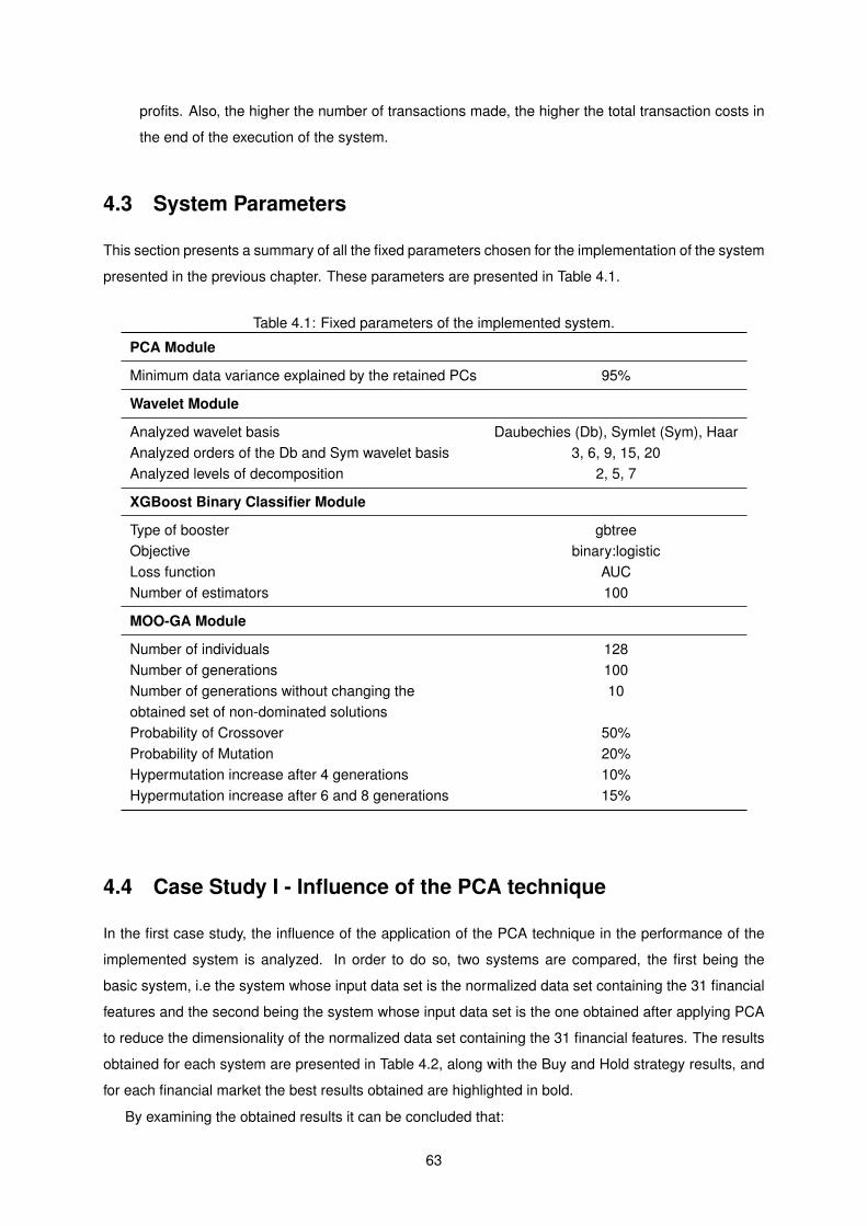
profits. Also, the higher the number of transactions made, the higher the total transaction costs in
the end of the execution of the system.
4.3 System Parameters
This section presents a summary of all the fixed parameters chosen for the implementation of the system
presented in the previous chapter. These parameters are presented in Table 4.1.
Table 4.1: Fixed parameters of the implemented system.
PCA Module
Minimum data variance explained by the retained PCs 95%
Wavelet Module
Analyzed wavelet basis Daubechies (Db), Symlet (Sym), HaarAnalyzed orders of the Db and Sym wavelet basis 3, 6, 9, 15, 20Analyzed levels of decomposition 2, 5, 7
XGBoost Binary Classifier Module
Type of booster gbtreeObjective binary:logisticLoss function AUCNumber of estimators 100
MOO-GA Module
Number of individuals 128Number of generations 100Number of generations without changing the 10obtained set of non-dominated solutionsProbability of Crossover 50%Probability of Mutation 20%Hypermutation increase after 4 generations 10%Hypermutation increase after 6 and 8 generations 15%
4.4 Case Study I - Influence of the PCA technique
In the first case study, the influence of the application of the PCA technique in the performance of the
implemented system is analyzed. In order to do so, two systems are compared, the first being the
basic system, i.e the system whose input data set is the normalized data set containing the 31 financial
features and the second being the system whose input data set is the one obtained after applying PCA
to reduce the dimensionality of the normalized data set containing the 31 financial features. The results
obtained for each system are presented in Table 4.2, along with the Buy and Hold strategy results, and
for each financial market the best results obtained are highlighted in bold.
By examining the obtained results it can be concluded that:
63
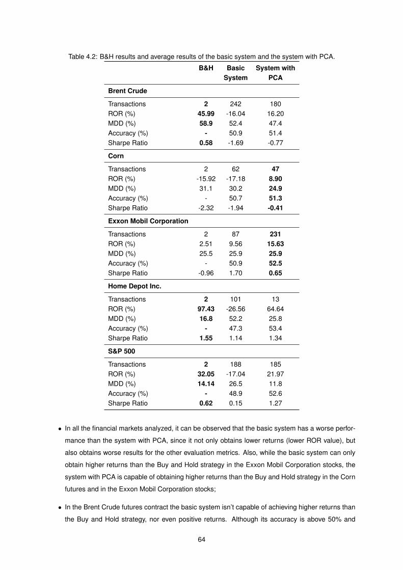
Table 4.2: B&H results and average results of the basic system and the system with PCA.
B&H Basic System withSystem PCA
Brent Crude
Transactions 2 242 180ROR (%) 45.99 -16.04 16.20MDD (%) 58.9 52.4 47.4Accuracy (%) - 50.9 51.4Sharpe Ratio 0.58 -1.69 -0.77
Corn
Transactions 2 62 47ROR (%) -15.92 -17.18 8.90MDD (%) 31.1 30.2 24.9Accuracy (%) - 50.7 51.3Sharpe Ratio -2.32 -1.94 -0.41
Exxon Mobil Corporation
Transactions 2 87 231ROR (%) 2.51 9.56 15.63MDD (%) 25.5 25.9 25.9Accuracy (%) - 50.9 52.5Sharpe Ratio -0.96 1.70 0.65
Home Depot Inc.
Transactions 2 101 13ROR (%) 97.43 -26.56 64.64MDD (%) 16.8 52.2 25.8Accuracy (%) - 47.3 53.4Sharpe Ratio 1.55 1.14 1.34
S&P 500
Transactions 2 188 185ROR (%) 32.05 -17.04 21.97MDD (%) 14.14 26.5 11.8Accuracy (%) - 48.9 52.6Sharpe Ratio 0.62 0.15 1.27
• In all the financial markets analyzed, it can be observed that the basic system has a worse perfor-
mance than the system with PCA, since it not only obtains lower returns (lower ROR value), but
also obtains worse results for the other evaluation metrics. Also, while the basic system can only
obtain higher returns than the Buy and Hold strategy in the Exxon Mobil Corporation stocks, the
system with PCA is capable of obtaining higher returns than the Buy and Hold strategy in the Corn
futures and in the Exxon Mobil Corporation stocks;
• In the Brent Crude futures contract the basic system isn’t capable of achieving higher returns than
the Buy and Hold strategy, nor even positive returns. Although its accuracy is above 50% and
64
its MDD is slightly lower than the one obtained in the Buy and Hold strategy, the Sharpe ratio is
lower, meaning that the system is incurring in trades with an high risk level. The system with PCA
achieves higher returns than the basic system but not high enough to surpass the ones obtained
in the Buy and Hold strategy. Its MDD is lower than in the other two strategies but the Sharpe
ratio is still lower than the one obtained in the Buy and Hold strategy meaning that while it is less
risky than the basic system, it is riskier than the Buy and Hold strategy, however since it has the
lowest MDD, the maximum loss from a peak would be lower. The system with PCA also performs
less trades than the basic system and achieves an higher accuracy, contributing to the increase of
ROR;
• The Corn futures contract is a financial market where the basic system has a similar performance
to the Buy and Hold strategy, achieving slightly lower returns but having a lower MDD and an
higher Sharpe Ratio. However, with the introduction of PCA, the system can obtain considerably
higher returns than the Buy and Hold strategy, while at the same time decreasing even more the
MDD and increasing the Sharpe ratio, meaning that there is a lower level of risk associated with
the trades made by this system. The accuracy is also higher and less trades are made, meaning
that some irrelevant trades that were made by the basic system were not made by the system with
PCA, which also contributes to the fact that the returns obtained are higher. One important thing
to note is that, similarly to the Buy and Hold strategy for financial markets with a positive trend,
for financial markets that have a negative trend like the Corn futures contract, the Short and Hold
strategy can be taken, which performs a short in the beginning, therefore increasing its value over
time since the asset’s value is decreasing. Although the system with PCA obtains higher returns
than the Buy and Hold strategy, if the Short and Hold strategy was used (obtaining a ROR of
15.92%), the system with PCA couldn’t obtain higher returns;
• In the Exxon Mobil Corporation stocks, the basic system is capable of achieving higher returns,
a lower MDD and an higher Sharpe ratio than the Buy and Hold strategy. The system with PCA
performs even better than the basic system, achieving higher returns and obtaining an higher
accuracy value even with more trades made, showing that the use of PCA allowed the system to
discover more profitable trades. However, the MDD value is the same in the two systems and the
Sharpe ratio is higher in the basic system, meaning that in the system with PCA, although it makes
more profitable trades, these trades also contribute to the increase of the risk level;
• In the Home Depot Inc. stocks, although the system with PCA doesn’t achieve higher returns
than the Buy and Hold strategy, the basic system obtains considerably lower returns than the
system with PCA, achieving a negative ROR. With respect to the other evaluation metrics, it can
be observed that the basic system also achieves lower accuracy and Sharpe ratio and has a MDD
of more than double the one obtained in the system with PCA, meaning that not only more than
half of its predictions are wrong, the level of risk associated to the trades made is also very high;
• In the S&P 500 index, the conclusions are very similar to the ones made on the Home Depot Inc.
stocks. The basic system doesn’t achieve higher returns than the Buy and Hold strategy and has a
65
negative ROR. The MDD and Sharpe ratio values are also worse and added to these results is the
fact that the accuracy is also lower than 50%, meaning that its predictions are making the system
incur in unnecessary and risky trades that consequently result in lower returns. In the system with
PCA the accuracy rises above 50% and although it doesn’t achieve higher returns than the Buy
and Hold strategy, the MDD is lower and the Sharpe ratio is higher, meaning that there is a lower
level of risk in the trades made.
Therefore, it can be concluded that the dimensionality reduction using the PCA technique plays
an important role in improving the performance of the system since it allows not only to obtain higher
returns, but also to achieve higher accuracy values meaning that it allows the XGBoost binary classifier
to produce less complex models capable of a good generalization ability to unseen data and helping
in avoiding overfitting the training data, this way allowing the system to achieve higher returns than the
Buy and Hold strategy in the all the analyzed markets with the exception of the Brent Crude futures,
Home Depot Inc. and the S&P 500 that are the markets with the highest ROR. However, in these three
financial markets, the use of the dimensionality reduction is vital for the system to obtain positive returns
since in the basic system the generalization capacity wasn’t good enough to classify correctly the test
set and from the observation of the return plots for the Home Depot Inc. stocks and S&P 500 Index, it
can be observed that the basic system performs well until nearly half of the testing period but as soon
as the close price starts to rise the system isn’t capable of following this trend which is related to the fact
that overfitting occurs and therefore since these high close prices weren’t present in the training set the
system isn’t capable of generalizing well to these values and ends up performing wrong trades. Without
the application of the PCA the system can only achieve higher returns than the Buy and Hold strategy in
the Exxon Mobil Corporation stocks. Furthermore, the use of the PCA technique also allows the system
to obtain an higher Sharpe ratio and a lower MDD in the Corn futures contract, in Home Depot Inc.
and in the S&P 500 index, which means that the solutions obtained generate good returns with lower
associated risk to the trades made, when compared to the basic system and the Buy and Hold strategy.
A graphical representation of the comparison of the returns obtained by the Buy and Hold strategy,
by the basic system and by the system with PCA is presented in Figure 4.1 and Figure 4.2 for the Corn
futures contract and Exxon Mobil Corporation stocks respectively, for the testing period and it can be
observed that, as mentioned before, with the introduction of the PCA the system is capable of obtaining
higher returns. The plots obtained for the remaining analyzed financial markets are present in Appendix
A.
4.5 Case Study II - Influence of the DWT denoise
In the second case study, the importance of the order of the chosen wavelet basis in the DWT, as
well as the chosen decomposition level, in the performance of the system is analyzed. In order to do
so, for each wavelet basis analyzed, a set of different orders and levels of decomposition are tested.
The results obtained for each system are presented in Table 4.3, along with the Buy and Hold strategy
results, and for each financial market the best results obtained are highlighted in bold. Since presenting
66
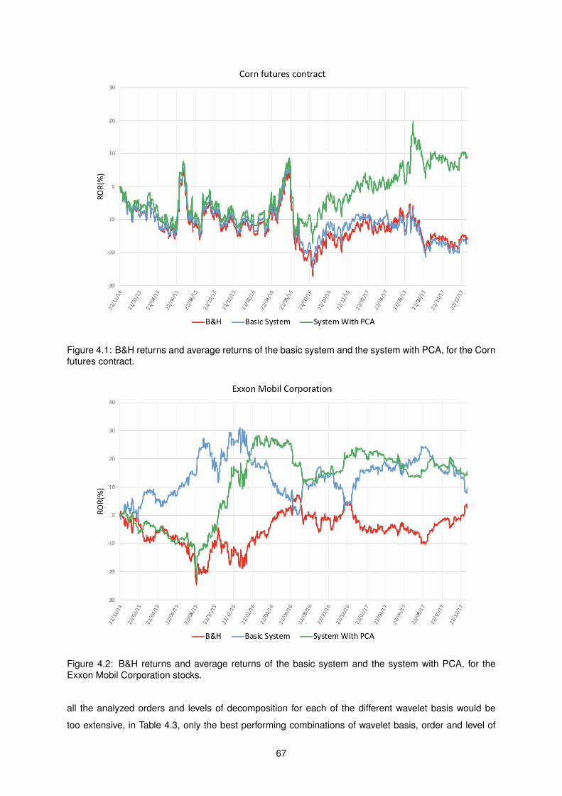
Figure 4.1: B&H returns and average returns of the basic system and the system with PCA, for the Cornfutures contract.
Figure 4.2: B&H returns and average returns of the basic system and the system with PCA, for theExxon Mobil Corporation stocks.
all the analyzed orders and levels of decomposition for each of the different wavelet basis would be
too extensive, in Table 4.3, only the best performing combinations of wavelet basis, order and level of
67
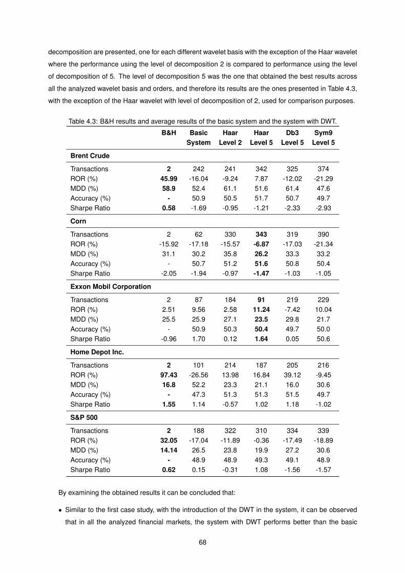
decomposition are presented, one for each different wavelet basis with the exception of the Haar wavelet
where the performance using the level of decomposition 2 is compared to performance using the level
of decomposition of 5. The level of decomposition 5 was the one that obtained the best results across
all the analyzed wavelet basis and orders, and therefore its results are the ones presented in Table 4.3,
with the exception of the Haar wavelet with level of decomposition of 2, used for comparison purposes.
Table 4.3: B&H results and average results of the basic system and the system with DWT.
B&H Basic Haar Haar Db3 Sym9System Level 2 Level 5 Level 5 Level 5
Brent Crude
Transactions 2 242 241 342 325 374ROR (%) 45.99 -16.04 -9.24 7.87 -12.02 -21.29MDD (%) 58.9 52.4 61.1 51.6 61.4 47.6Accuracy (%) - 50.9 50.5 51.7 50.7 49.7Sharpe Ratio 0.58 -1.69 -0.95 -1.21 -2.33 -2.93
Corn
Transactions 2 62 330 343 319 390ROR (%) -15.92 -17.18 -15.57 -6.87 -17.03 -21.34MDD (%) 31.1 30.2 35.8 26.2 33.3 33.2Accuracy (%) - 50.7 51.2 51.6 50.8 50.4Sharpe Ratio -2.05 -1.94 -0.97 -1.47 -1.03 -1.05
Exxon Mobil Corporation
Transactions 2 87 184 91 219 229ROR (%) 2.51 9.56 2.58 11.24 -7.42 10.04MDD (%) 25.5 25.9 27.1 23.5 29.8 21.7Accuracy (%) - 50.9 50.3 50.4 49.7 50.0Sharpe Ratio -0.96 1.70 0.12 1.64 0.05 50.6
Home Depot Inc.
Transactions 2 101 214 187 205 216ROR (%) 97.43 -26.56 13.98 16.84 39.12 -9.45MDD (%) 16.8 52.2 23.3 21.1 16.0 30.6Accuracy (%) - 47.3 51.3 51.3 51.5 49.7Sharpe Ratio 1.55 1.14 -0.57 1.02 1.18 -1.02
S&P 500
Transactions 2 188 322 310 334 339ROR (%) 32.05 -17.04 -11.89 -0.36 -17.49 -18.89MDD (%) 14.14 26.5 23.8 19.9 27.2 30.6Accuracy (%) - 48.9 48.9 49.3 49.1 48.9Sharpe Ratio 0.62 0.15 -0.31 1.08 -1.56 -1.57
By examining the obtained results it can be concluded that:
• Similar to the first case study, with the introduction of the DWT in the system, it can be observed
that in all the analyzed financial markets, the system with DWT performs better than the basic
68
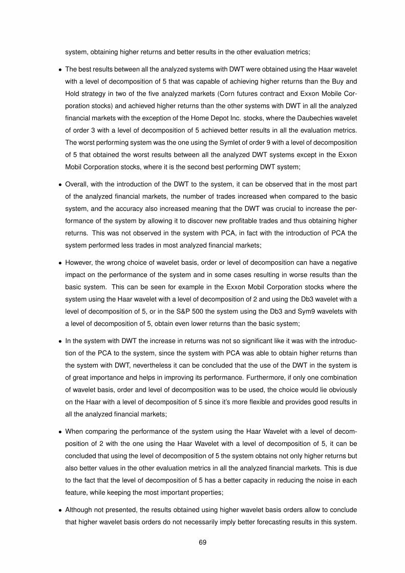
system, obtaining higher returns and better results in the other evaluation metrics;
• The best results between all the analyzed systems with DWT were obtained using the Haar wavelet
with a level of decomposition of 5 that was capable of achieving higher returns than the Buy and
Hold strategy in two of the five analyzed markets (Corn futures contract and Exxon Mobile Cor-
poration stocks) and achieved higher returns than the other systems with DWT in all the analyzed
financial markets with the exception of the Home Depot Inc. stocks, where the Daubechies wavelet
of order 3 with a level of decomposition of 5 achieved better results in all the evaluation metrics.
The worst performing system was the one using the Symlet of order 9 with a level of decomposition
of 5 that obtained the worst results between all the analyzed DWT systems except in the Exxon
Mobil Corporation stocks, where it is the second best performing DWT system;
• Overall, with the introduction of the DWT to the system, it can be observed that in the most part
of the analyzed financial markets, the number of trades increased when compared to the basic
system, and the accuracy also increased meaning that the DWT was crucial to increase the per-
formance of the system by allowing it to discover new profitable trades and thus obtaining higher
returns. This was not observed in the system with PCA, in fact with the introduction of PCA the
system performed less trades in most analyzed financial markets;
• However, the wrong choice of wavelet basis, order or level of decomposition can have a negative
impact on the performance of the system and in some cases resulting in worse results than the
basic system. This can be seen for example in the Exxon Mobil Corporation stocks where the
system using the Haar wavelet with a level of decomposition of 2 and using the Db3 wavelet with a
level of decomposition of 5, or in the S&P 500 the system using the Db3 and Sym9 wavelets with
a level of decomposition of 5, obtain even lower returns than the basic system;
• In the system with DWT the increase in returns was not so significant like it was with the introduc-
tion of the PCA to the system, since the system with PCA was able to obtain higher returns than
the system with DWT, nevertheless it can be concluded that the use of the DWT in the system is
of great importance and helps in improving its performance. Furthermore, if only one combination
of wavelet basis, order and level of decomposition was to be used, the choice would lie obviously
on the Haar with a level of decomposition of 5 since it’s more flexible and provides good results in
all the analyzed financial markets;
• When comparing the performance of the system using the Haar Wavelet with a level of decom-
position of 2 with the one using the Haar Wavelet with a level of decomposition of 5, it can be
concluded that using the level of decomposition of 5 the system obtains not only higher returns but
also better values in the other evaluation metrics in all the analyzed financial markets. This is due
to the fact that the level of decomposition of 5 has a better capacity in reducing the noise in each
feature, while keeping the most important properties;
• Although not presented, the results obtained using higher wavelet basis orders allow to conclude
that higher wavelet basis orders do not necessarily imply better forecasting results in this system.
69

The same happens with the decomposition level, although with an higher decomposition level more
noise can be removed from the signal, this often results in removing important signal properties that
consequently harm the forecasting task. In general, when there was an increase in performance
for a financial market, the increase was only marginal and, most important, the increase wasn’t
verified in all the analyzed financial markets, therefore due to this and due to the fact that when
using higher decomposition levels, the computation time increases, the level of decomposition
considered optimal for the system was 5.
A graphical representation of the comparison of the returns obtained by the Buy and Hold strategy,
by the basic system and by the system with the Haar wavelet and a level of decomposition of 5 is
presented in Figure 4.3 and Figure 4.4 for the Corn futures contract and Exxon Mobil Corporation stocks
respectively, for the testing period and it can be observed that, although the returns are not as high
as the ones presented in the previous case study, the DWT has a positive influence on the system by
increasing the obtained returns. The plots obtained for the remaining analyzed financial markets are
present in Appendix B, using for each financial market the best system with DWT.
Figure 4.3: B&H returns and average returns of the basic system and the system with Haar wavelet witha level of decomposition of 5, for the Corn futures contract.
4.6 Case Study III - Combining PCA and DWT
In the third, and last case study, after having analyzed the importance of the PCA and DWT in increasing
the overall performance of the system when applied separately, the PCA and DWT techniques are now
combined together to achieve a system that not only performs dimensionality reduction to the financial
70
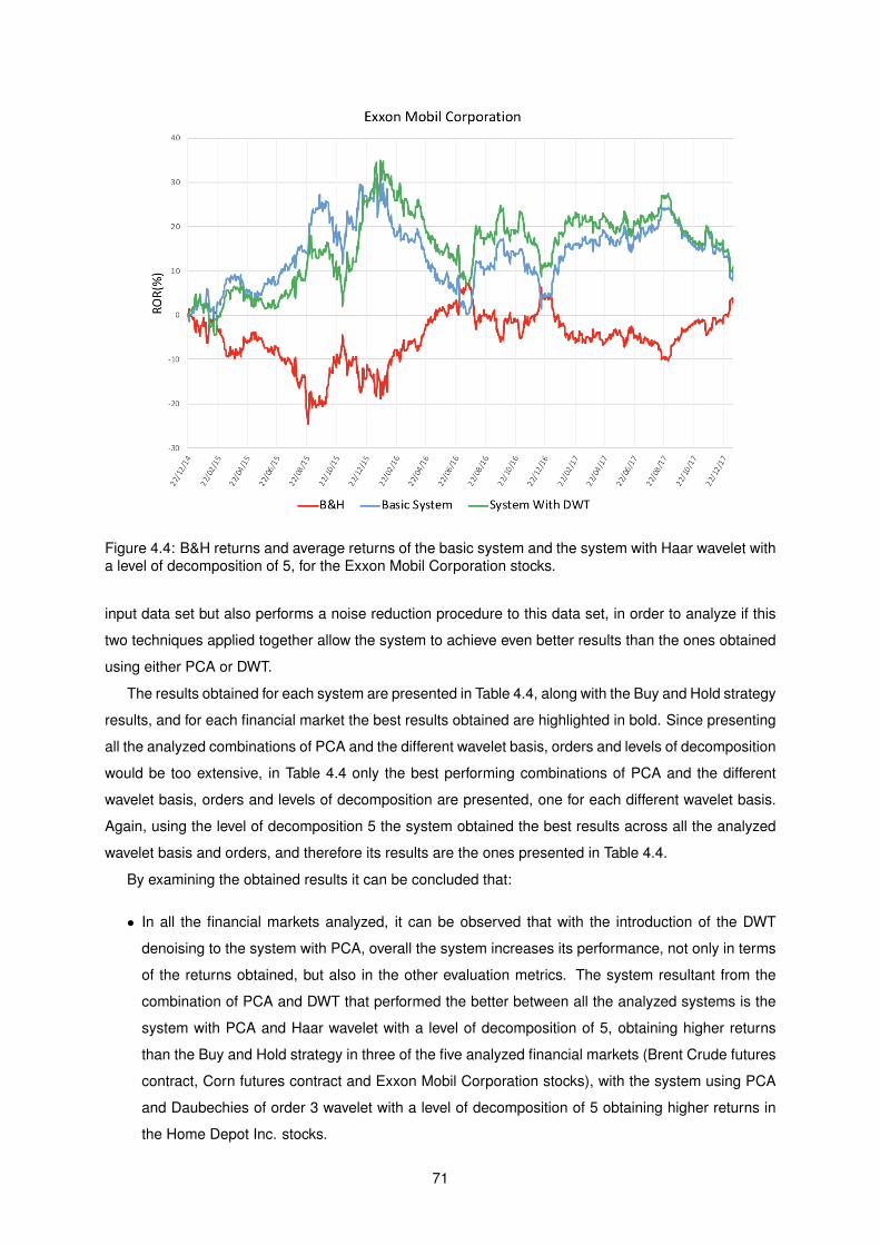
Figure 4.4: B&H returns and average returns of the basic system and the system with Haar wavelet witha level of decomposition of 5, for the Exxon Mobil Corporation stocks.
input data set but also performs a noise reduction procedure to this data set, in order to analyze if this
two techniques applied together allow the system to achieve even better results than the ones obtained
using either PCA or DWT.
The results obtained for each system are presented in Table 4.4, along with the Buy and Hold strategy
results, and for each financial market the best results obtained are highlighted in bold. Since presenting
all the analyzed combinations of PCA and the different wavelet basis, orders and levels of decomposition
would be too extensive, in Table 4.4 only the best performing combinations of PCA and the different
wavelet basis, orders and levels of decomposition are presented, one for each different wavelet basis.
Again, using the level of decomposition 5 the system obtained the best results across all the analyzed
wavelet basis and orders, and therefore its results are the ones presented in Table 4.4.
By examining the obtained results it can be concluded that:
• In all the financial markets analyzed, it can be observed that with the introduction of the DWT
denoising to the system with PCA, overall the system increases its performance, not only in terms
of the returns obtained, but also in the other evaluation metrics. The system resultant from the
combination of PCA and DWT that performed the better between all the analyzed systems is the
system with PCA and Haar wavelet with a level of decomposition of 5, obtaining higher returns
than the Buy and Hold strategy in three of the five analyzed financial markets (Brent Crude futures
contract, Corn futures contract and Exxon Mobil Corporation stocks), with the system using PCA
and Daubechies of order 3 wavelet with a level of decomposition of 5 obtaining higher returns in
the Home Depot Inc. stocks.
71
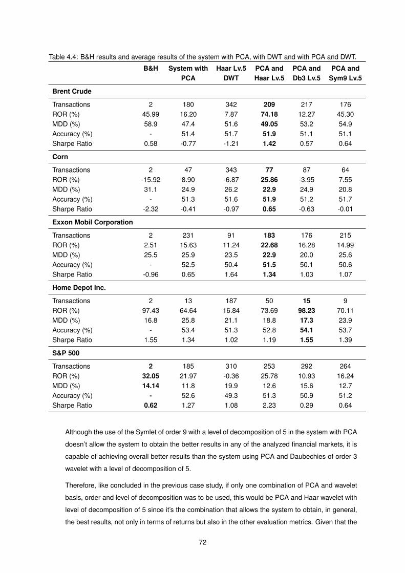
Table 4.4: B&H results and average results of the system with PCA, with DWT and with PCA and DWT.
B&H System with Haar Lv.5 PCA and PCA and PCA andPCA DWT Haar Lv.5 Db3 Lv.5 Sym9 Lv.5
Brent Crude
Transactions 2 180 342 209 217 176ROR (%) 45.99 16.20 7.87 74.18 12.27 45.30MDD (%) 58.9 47.4 51.6 49.05 53.2 54.9Accuracy (%) - 51.4 51.7 51.9 51.1 51.1Sharpe Ratio 0.58 -0.77 -1.21 1.42 0.57 0.64
Corn
Transactions 2 47 343 77 87 64ROR (%) -15.92 8.90 -6.87 25.86 -3.95 7.55MDD (%) 31.1 24.9 26.2 22.9 24.9 20.8Accuracy (%) - 51.3 51.6 51.9 51.2 51.7Sharpe Ratio -2.32 -0.41 -0.97 0.65 -0.63 -0.01
Exxon Mobil Corporation
Transactions 2 231 91 183 176 215ROR (%) 2.51 15.63 11.24 22.68 16.28 14.99MDD (%) 25.5 25.9 23.5 22.9 20.0 25.6Accuracy (%) - 52.5 50.4 51.5 50.1 50.6Sharpe Ratio -0.96 0.65 1.64 1.34 1.03 1.07
Home Depot Inc.
Transactions 2 13 187 50 15 9ROR (%) 97.43 64.64 16.84 73.69 98.23 70.11MDD (%) 16.8 25.8 21.1 18.8 17.3 23.9Accuracy (%) - 53.4 51.3 52.8 54.1 53.7Sharpe Ratio 1.55 1.34 1.02 1.19 1.55 1.39
S&P 500
Transactions 2 185 310 253 292 264ROR (%) 32.05 21.97 -0.36 25.78 10.93 16.24MDD (%) 14.14 11.8 19.9 12.6 15.6 12.7Accuracy (%) - 52.6 49.3 51.3 50.9 51.2Sharpe Ratio 0.62 1.27 1.08 2.23 0.29 0.64
Although the use of the Symlet of order 9 with a level of decomposition of 5 in the system with PCA
doesn’t allow the system to obtain the better results in any of the analyzed financial markets, it is
capable of achieving overall better results than the system using PCA and Daubechies of order 3
wavelet with a level of decomposition of 5.
Therefore, like concluded in the previous case study, if only one combination of PCA and wavelet
basis, order and level of decomposition was to be used, this would be PCA and Haar wavelet with
level of decomposition of 5 since it’s the combination that allows the system to obtain, in general,
the best results, not only in terms of returns but also in the other evaluation metrics. Given that the
72

Haar is the simplest wavelet, it is the more flexible one, meaning that it can be applied to signals
with different characteristics and achieve an acceptable performance in each one. Although with
the Daubechies and Symlet wavelets the resultant signal is smoother, the Haar wavelet allows for
a better detection of sudden changes in the signal which is a very important characteristic when
dealing with highly oscillating signals such as financial market signals;
• Overall, the best performing system combining PCA and DWT in each financial market achieved
better results than the other analyzed systems and the Buy and Hold strategy, except for the S&P
500 index in which the best performing final system obtained less 6.27% of returns but on the other
hand both the MDD and Sharpe ratio values were better, meaning that it produced a less risky
strategy. The financial market in which the best returns were obtained is the Corn futures contract
where the Buy and Hold strategy obtains a negative ROR and the best performing final system
obtains more 41.78% of returns. Also, the trading strategies obtained using the best performing
final system, in the most part of the cases, have an higher Sharpe ratio and a lower MDD, therefore
having a lower level of risk associated meaning that the proposed system not only allows to obtain
higher returns but also provides the user with solutions where the possible losses are lower and
less frequent;
• Furthermore, the obtained accuracy values in the system combining PCA and DWT are all above
50%, with the worst accuracy obtained being 51.5% in the Exxon Mobil Corporation stocks and the
best being 54.1% in the Home Depot Inc. stocks. Therefore, these obtained accuracy values prove
that, in contrast to the EMH theory, the financial markets aren’t purely chaotic and unforecastable,
meaning that a Machine Learning system developed to trade in financial markets can learn from
historical financial data and use some of the patterns learned in order to come up with trading
strategies that can be applied to more recent time periods and that perform better than random
guessing. It can be observed that in some financial markets, systems with lower accuracy can
sometimes obtain higher returns than other systems with an higher accuracy, this is related to the
ammount of trades made by the system and if it changes the position very often meaning that,
for example in an uptrend period a system that takes always the Long position can have a lower
accuracy than a system that changes its position more often to catch small variations in price
but that can end up performing irrelevant trades that the other system didn’t perform since it was
always taking the Long position.
Therefore, it can be concluded that the combination of the PCA and DWT denoising techniques
allows the system to obtain better results than the system using just PCA and the system using just
DWT. This is due to the fact that in this system the PCA reduces the dimension of the financial input
data set and the DWT performs a denoising to this reduced data set, which not only helps in avoiding
overfitting the training data, since there are less features in the data set, but also helps in removing some
irrelevant samples that could harm the system performance, therefore aiding the system in the learning
process and increasing its generalization ability. However, like already mentioned in the previous case
study, this increase in performance can only be verified when the appropriate wavelet basis, order and
73
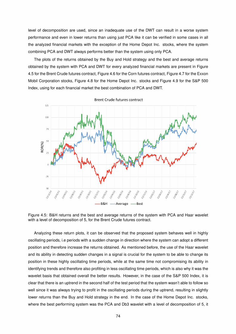
level of decomposition are used, since an inadequate use of the DWT can result in a worse system
performance and even in lower returns than using just PCA like it can be verified in some cases in all
the analyzed financial markets with the exception of the Home Depot Inc. stocks, where the system
combining PCA and DWT always performs better than the system using only PCA.
The plots of the returns obtained by the Buy and Hold strategy and the best and average returns
obtained by the system with PCA and DWT for every analyzed financial markets are present in Figure
4.5 for the Brent Crude futures contract, Figure 4.6 for the Corn futures contract, Figure 4.7 for the Exxon
Mobil Corporation stocks, Figure 4.8 for the Home Depot Inc. stocks and Figure 4.9 for the S&P 500
Index, using for each financial market the best combination of PCA and DWT.
Figure 4.5: B&H returns and the best and average returns of the system with PCA and Haar waveletwith a level of decomposition of 5, for the Brent Crude futures contract.
Analyzing these return plots, it can be observed that the proposed system behaves well in highly
oscillating periods, i.e periods with a sudden change in direction where the system can adopt a different
position and therefore increase the returns obtained. As mentioned before, the use of the Haar wavelet
and its ability in detecting sudden changes in a signal is crucial for the system to be able to change its
position in these highly oscillating time periods, while at the same time not compromising its ability in
identifying trends and therefore also profiting in less oscillating time periods, which is also why it was the
wavelet basis that obtained overall the better results. However, in the case of the S&P 500 Index, it is
clear that there is an uptrend in the second half of the test period that the system wasn’t able to follow so
well since it was always trying to profit in the oscillating periods during the uptrend, resulting in slightly
lower returns than the Buy and Hold strategy in the end. In the case of the Home Depot Inc. stocks,
where the best performing system was the PCA and Db3 wavelet with a level of decomposition of 5, it
74

Figure 4.6: B&H returns and the best and average returns of the system with PCA and Haar waveletwith a level of decomposition of 5, for the Corn futures contract.
Figure 4.7: B&H returns and the best and average returns of the system with PCA and Haar waveletwith a level of decomposition of 5, for the Exxon Mobil Corporation stocks.
can be observed that the system always followed the uptrend direction of the financial market and didn’t
perform many trades, this way achieving similar results to the Buy and Hold strategy.
75

Figure 4.8: B&H returns and the best and average returns of the system with PCA and Db3 wavelet witha level of decomposition of 5, for the Home Depot Inc. stocks.
Figure 4.9: B&H returns and the best and average returns of the system with PCA and Haar waveletwith a level of decomposition of 5, for the S&P 500 Index.
In the case of the Brent Crude futures contract and in the Exxon Mobil Corporation stocks, it is clear
from the observation of the respective return plots that there is a high volatility in the first half of the
76
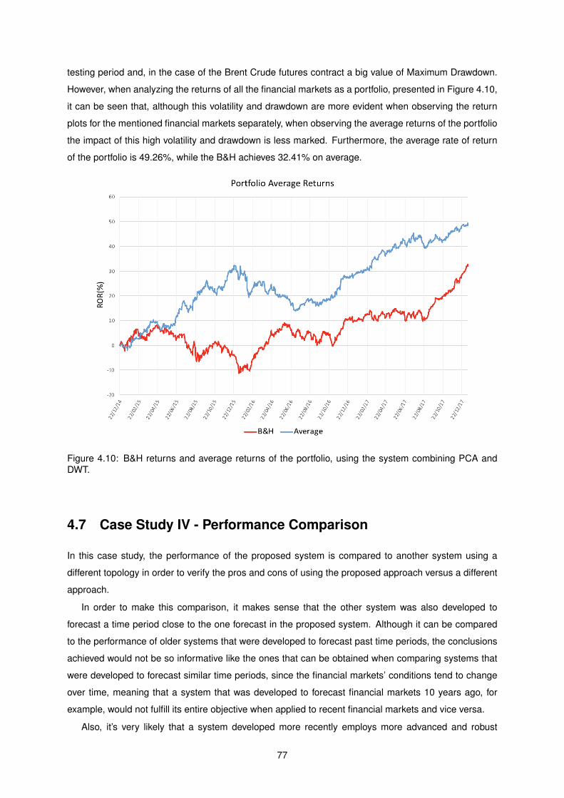
testing period and, in the case of the Brent Crude futures contract a big value of Maximum Drawdown.
However, when analyzing the returns of all the financial markets as a portfolio, presented in Figure 4.10,
it can be seen that, although this volatility and drawdown are more evident when observing the return
plots for the mentioned financial markets separately, when observing the average returns of the portfolio
the impact of this high volatility and drawdown is less marked. Furthermore, the average rate of return
of the portfolio is 49.26%, while the B&H achieves 32.41% on average.
Figure 4.10: B&H returns and average returns of the portfolio, using the system combining PCA andDWT.
4.7 Case Study IV - Performance Comparison
In this case study, the performance of the proposed system is compared to another system using a
different topology in order to verify the pros and cons of using the proposed approach versus a different
approach.
In order to make this comparison, it makes sense that the other system was also developed to
forecast a time period close to the one forecast in the proposed system. Although it can be compared
to the performance of older systems that were developed to forecast past time periods, the conclusions
achieved would not be so informative like the ones that can be obtained when comparing systems that
were developed to forecast similar time periods, since the financial markets’ conditions tend to change
over time, meaning that a system that was developed to forecast financial markets 10 years ago, for
example, would not fulfill its entire objective when applied to recent financial markets and vice versa.
Also, it’s very likely that a system developed more recently employs more advanced and robust
77
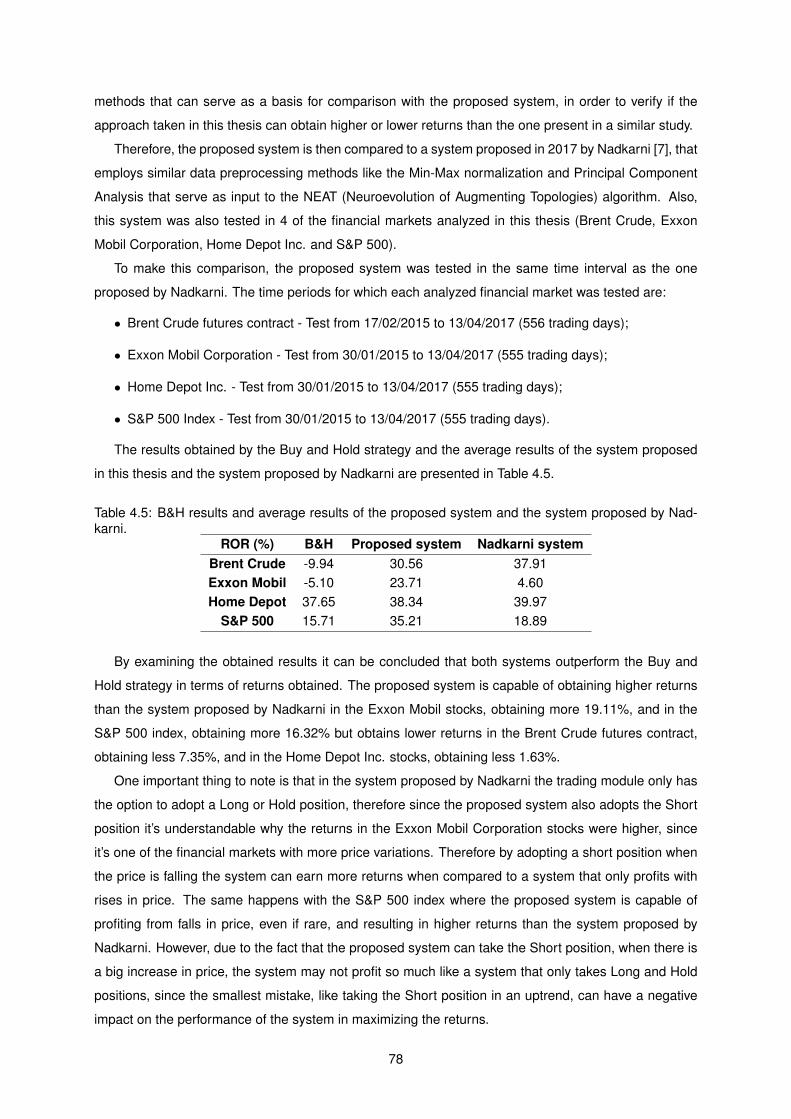
methods that can serve as a basis for comparison with the proposed system, in order to verify if the
approach taken in this thesis can obtain higher or lower returns than the one present in a similar study.
Therefore, the proposed system is then compared to a system proposed in 2017 by Nadkarni [7], that
employs similar data preprocessing methods like the Min-Max normalization and Principal Component
Analysis that serve as input to the NEAT (Neuroevolution of Augmenting Topologies) algorithm. Also,
this system was also tested in 4 of the financial markets analyzed in this thesis (Brent Crude, Exxon
Mobil Corporation, Home Depot Inc. and S&P 500).
To make this comparison, the proposed system was tested in the same time interval as the one
proposed by Nadkarni. The time periods for which each analyzed financial market was tested are:
• Brent Crude futures contract - Test from 17/02/2015 to 13/04/2017 (556 trading days);
• Exxon Mobil Corporation - Test from 30/01/2015 to 13/04/2017 (555 trading days);
• Home Depot Inc. - Test from 30/01/2015 to 13/04/2017 (555 trading days);
• S&P 500 Index - Test from 30/01/2015 to 13/04/2017 (555 trading days).
The results obtained by the Buy and Hold strategy and the average results of the system proposed
in this thesis and the system proposed by Nadkarni are presented in Table 4.5.
Table 4.5: B&H results and average results of the proposed system and the system proposed by Nad-karni.
ROR (%) B&H Proposed system Nadkarni systemBrent Crude -9.94 30.56 37.91Exxon Mobil -5.10 23.71 4.60Home Depot 37.65 38.34 39.97
S&P 500 15.71 35.21 18.89
By examining the obtained results it can be concluded that both systems outperform the Buy and
Hold strategy in terms of returns obtained. The proposed system is capable of obtaining higher returns
than the system proposed by Nadkarni in the Exxon Mobil stocks, obtaining more 19.11%, and in the
S&P 500 index, obtaining more 16.32% but obtains lower returns in the Brent Crude futures contract,
obtaining less 7.35%, and in the Home Depot Inc. stocks, obtaining less 1.63%.
One important thing to note is that in the system proposed by Nadkarni the trading module only has
the option to adopt a Long or Hold position, therefore since the proposed system also adopts the Short
position it’s understandable why the returns in the Exxon Mobil Corporation stocks were higher, since
it’s one of the financial markets with more price variations. Therefore by adopting a short position when
the price is falling the system can earn more returns when compared to a system that only profits with
rises in price. The same happens with the S&P 500 index where the proposed system is capable of
profiting from falls in price, even if rare, and resulting in higher returns than the system proposed by
Nadkarni. However, due to the fact that the proposed system can take the Short position, when there is
a big increase in price, the system may not profit so much like a system that only takes Long and Hold
positions, since the smallest mistake, like taking the Short position in an uptrend, can have a negative
impact on the performance of the system in maximizing the returns.
78
Chapter 5
Conclusions
In this thesis, a system combining Principal Component Analysis and Discrete Wavelet Transform for
dimensionality reduction and noise reduction, respectively, with an XGBoost binary classifier optimized
using a Multi-Objective Optimization Genetic Algorithm is presented, with the purpose of achieving the
maximum returns possible, while minimizing the level of risk in the trading strategy.
The main stages of the data preprocessing are the Principal Component Analysis that, after the data
is normalized, reduces the high dimensional input financial data set to a data set with a lower dimension
and the Discrete Wavelet Transform that further reduces the noise present in each feature of this reduced
data set. Then, this data set is fed to the XGBoost binary classifier responsible to discover patterns in
the training data that can be used in order to make correct predictions in unseen data and generate a
trading signal that can achieve good returns with a low level of risk. The XGBoost binary classifier has
its hyperparameters optimized using a Multi-Objective Optimization Genetic Algorithm in order to make
sure that, for each analyzed financial market, the performance of the XGBoost binary classifier is the
highest possible.
The developed system was tested in five different markets, each with its own characteristics, in order
to conclude if the system was capable or not of dealing with different market behaviours and even so
maintain its performance regardless of the financial market’s behaviour. The results obtained show
that the system is very robust to this change of financial market’s characteristics, obtaining a good
performance in the analyzed financial markets.
5.1 Conclusions
In this work, the performance of the system using three data preprocessing methods is compared in
order to determine which methods provide the best results.
First, the system without any data preprocessing method, besides the data normalization, is com-
pared to a system using PCA to reduce the dimension of the financial input data set, while still retaining
the main characteristics of the original data set. The results obtained show that the use of PCA for
dimensionality reduction allows the system to increase its performance, obtaining positive returns in all
79

the analyzed financial markets and higher returns than the Buy and Hold strategy in two of them, while
without the PCA the system was only capable of achieving higher returns than the Buy and Hold strategy
in one analyzed financial market. With the dimensionality reduction technique, the number of features in
the financial data set, which originally has 31 features, is considerably reduced, allowing the system to
improve its generalization ability and making it less prone to overfitting.
Then, the system without any data preprocessing method, besides the data normalization, is com-
pared to a system using the DWT to perform noise reduction in the financial input data set. The results
obtained show that this technique, although not having the same importance in improving the results
like the PCA does, is useful to allow the system to perform more profitable trades as well as reduce the
level of risk, therefore improving the performance of the system.
Finally, having concluded that both the PCA and DWT have a great importance in improving the
performance of the system, these two techniques are combined in order to create the final system. The
final system is able to obtain higher returns than both the system with PCA and the system with DWT.
Furthermore, it also obtains higher returns than the Buy and Hold strategy, except in the S&P 500 index.
By combining the PCA with the DWT, the input financial data set has its dimension reduced and some
irrelevant samples are discarded through the noise reduction phase, resulting in an input financial data
set that will not only make the system less prone to overfitting and enhance its generalization capabilities
but also will aid the system in the training phase since some samples that could have a negative impact
on the model fitting are removed through the noise reduction.
From the analysis of the results obtained using the system combining PCA and DWT, it was observed
that the system performed very well on high oscillating time periods, i.e time periods where the price
of the stock has many inversions, meaning that the system, by alternating between the Long and Short
positions, can make profitable trades that end up being decisive to obtain high returns. This is due to
the fact that the Haar wavelet has the ability of detecting sudden changes in a signal, this way obtaining
higher returns than the other analyzed wavelet basis in highly oscillating financial markets.
One important conclusion derived from the obtained results using both the analyzed systems is that,
in some financial markets, the three analyzed systems were able to obtain an accuracy higher than 50%
in its predictions. In fact, in both the system with PCA and the system with PCA and DWT (in the best
performing combination of PCA and wavelet basis, order and level), in all the analyzed financial markets
an accuracy of more than 50% was obtained, meaning that, in contrast to the EMH, it is possible to
develop a Machine Learning to trade in financial markets that is able to perform better than random
guessing.
5.2 Future Work
In order to improve the performance of the proposed system described in this thesis, there are some
approaches that can be explored that can also be of great use when solving similar problems, and they
are:
• The use of the Wavelet Packet Transform, which is similar to the DWT but while in the DWT
80

only the approximation coefficients are decomposed, in the Wavelet Packet Transform both the
approximation coefficients and the detail coefficients are decomposed. The comparison of these
two methods would be interesting in order to observe which produces the better results;
• The automatic choose of which wavelet basis, order and level of decomposition to use, by the
means of using it as a gene of the GA. For each analyzed financial market the system would
automatically choose the best parameters for the wavelet that performs the best;
• Instead of using a GA, using Bayesian Optimization which is a promising new method for optimiza-
tion problems that constructs a posterior distribution of functions (Gaussian Process) that best
describes the target function to optimize;
• The use of different fitness functions for the MOO-GA is very important in order to verify if the
performance of the system can be further improved with fitness functions that analyze different
metrics, for example one that has into account the risk and the number of days spent in the market
like the Risk Return Ratio (RRR);
• In this system, the MOO-GA parameters were fixed in all the case studies, a more in-depth analysis
of the influence of the MOO-GA parameters variation could prove itself useful in order to verify if
better results can be obtained using a different set of parameters;
• In order to try to overcome the high volatility and big drawdown values experienced in some ana-
lyzed financial markets, the use of the VIX indicator in the input data set is a possible way to further
improve the returns of the system in these periods.
81
Bibliography
[1] B. G. Malkiel. The efficient market hypothesis and its critics. Journal of Economic Perspectives, 17
(1):59–82, 2003.
[2] S. B. Achelis. Technical Analysis from A to Z. McGraw-Hill Education, 2nd edition, 2013. ISBN:978-
0071826297.
[3] Y. He, K. Fataliyev, and L. Wang. Feature selection for stock market analysis. Neural Information
Processing. ICONIP 2013. Lecture Notes in Computer Science, 8227:737–744, 2013.
[4] L. B. Almeida. An introduction to principal components analysis. Instituto Superior Tecnico. Dec,
2015.
[5] I. T. Jolliffe. A note on the use of principal components in regression. Applied Statistics, 31(3):
300–303, 1982.
[6] X. Zhong and D. Enke. Forecasting daily stock market return using dimensionality reduction. Expert
Systems with Applications, 67(C):126–139, Jan. 2017.
[7] J. Nadkarni and R. Neves. Combining neuroevolution and principal component analysis to trade in
the financial markets. Expert Systems with Applications, 103:184–195, 2018.
[8] B. Weng. Application of machine learning techniques for stock market prediction. PhD thesis,
Auburn University. May, 2017.
[9] I. T. Jolliffe. Principal Component Analysis. Springer, 2nd edition, 2002. ISBN:978-0387954424.
[10] A. Galli, G. Heydt, and P. Ribeiro. Exploring the power of wavelet analysis. IEEE Computer Appli-
cations in Power, 9(4):737–744, Oct. 1996.
[11] S. Schluter and C. Deuschle. Wavelet-based forecasting of arima time series - an empirical com-
parison of different methods. Managerial Economics, 15(1):107–131, 2014.
[12] P. S. Addison. The Illustrated Wavelet Transform Handbook: Introductory Theory and Applica-
tions in Science, Engineering, Medicine and Finance. CRC Press, 1st edition, 2002. ISBN:978-
0750306928.
[13] S. Mallat. A theory for multiresolution signal decomposition: the wavelet representation. IEEE
Transactions on Pattern Analysis and Machine Intelligence, 11(7):674–693, July 1989.
82

[14] B. Rajoub. An efficient coding algorithm for the compression of ecg signals using the wavelet
transform. IEEE Transactions on Biomedical Engineering, 49(4):355–362, Apr. 2002.
[15] L. Ephremidze, A. Gamkrelidze, and E. Lagvilava. An approximation of daubechies wavelet ma-
trices by perfect reconstruction filter banks with rational coefficients. Advances in Computational
Mathematics, 38(1):147–158, Jan. 2013.
[16] F. Keinert. Wavelets and multiwavelets. Chapman & Hall/CRC, 2nd edition, 2004. ISBN:1-58488-
304-9.
[17] D. L. Donoho and I. M. Johnstone. Ideal spatial adaptation by wavelet shrinkage. Biometrika, 81
(3):425–455, Sept. 1994.
[18] S. Chang, B. Yu, and M. Vetterli. Adaptive wavelet thresholding for image denoising and compres-
sion. IEEE Transactions on Image Processing, 9(9):1532–1546, Sept. 2000.
[19] D. L. Donoho, I. M. Johnstone, G. Kerkyacharian, and D. Picard. Wavelet shrinkage: Asymptopia?
Journal of the Royal Statistical Society, Ser. B, pages 371–394, 1995.
[20] T.-J. Hsieh, H.-F. Hsiao, and W.-C. Yeh. Forecasting stock markets using wavelet transforms and
recurrent neural networks: An integrated system based on artificial bee colony algorithm. Applied
Soft Computing, 11(2):2510–2525, Mar. 2011.
[21] J. C. P. M’ng and M. Mehralizadeh. Forecasting east asian indices futures via a novel hybrid of
wavelet-pca denoising and artificial neural network models. PLoS ONE, 11(6), June 2016.
[22] S. Mallat. A Wavelet Tour of Signal Processing - The Sparse Way. Academic Press, 3rd edition,
2008. ISBN: 978-0123743701.
[23] R. E. Schapire. A brief introduction to boosting. Proceedings of the Sixteenth International Joint
Conference on Artificial Intelligence, 2:1401–1406, July 1999.
[24] P. Buhlmann. Bagging, boosting and ensemble methods. Handbook of Computational Statistics,
pages 985–1022, 2012.
[25] Y. Freund and R. E. Schapire. A decision-theoretic generalization of on-line learning and an appli-
cation to boosting. Journal of Computer and System Sciences, 55(1):119–139, Aug. 1997.
[26] T. Chen and C. Guestrin. Xgboost: A scalable tree boosting system. Proceedings of the 22nd acm
sigkdd international conference on knowledge discovery and data mining, pages 785–794, 2016.
[27] J. H. Friedman. Greedy function approximation: A gradient boosting machine. The Annals of
Statistics, 29(5):1189–1232, Oct. 2001.
[28] L. Breiman, J. Friedman, C. J. Stone, and R. Olshen. Classification and Regression Trees. Taylor
& Francis, 1984. ISBN:978-0412048418.
83
[29] Introduction to Boosted Trees. http://xgboost.readthedocs.io/en/latest/model.html, 2015.
[Online; accessed 21-February-2018].
[30] S. Dey, Y. Kumar, S. Saha, and S. Basak. Forecasting to classification: Predicting the direction of
stock market price using xtreme gradient boosting. Applied Soft Computing, Oct. 2016.
[31] W. Wang, Y. Shi, G. Lyu, and W. Deng. Electricity consumption prediction using xgboost based
on discrete wavelet transform. 2017 2nd International Conference on Artificial Intelligence and
Engineering Applications (AIEA 2017), 2017.
[32] J. H. Holland. Adaptation in Natural and Artificial Systems: An Introductory Analysis with Applica-
tions to Biology, Control and Artificial Intelligence. MIT Press, 1992. ISBN:978-0262082136.
[33] M. Mitchell. An Introduction to Genetic Algorithms. MIT Press, 1996. ISBN:978-0262133166.
[34] P. Ngatchou, A. Zarei, and A. El-Sharkawi. Pareto multi objective optimization. Proceedings of the
13th International Conference on Intelligent Systems Application to Power Systems, Nov. 2005.
[35] K. Deb. Multi-objective optimization using evolutionary algorithms: An introduction. Multi-objective
evolutionary optimisation for product design and manufacturing, pages 1–24, Feb. 2011.
[36] A. Konak, D. W. Coit, and A. E.Smith. Multi-objective optimization using genetic algorithms: A
tutorial. Reliability Engineering & System Safety, 91(9):992–1007, Sept. 2006.
[37] K. Deb, A. Pratap, S. Agarwal, and T. Meyarivan. A fast and elitist multiobjective genetic algorithm:
Nsga-ii. IEEE Transactions on Evolutionary Computation, 6(2):182–197, Apr. 2002.
[38] A. Pimenta, C. A. L. Nametala, F. G. Guimaraes, and E. G. Carrano. An automated investing
method for stock market based on multiobjective genetic programming. Computational Economics,
pages 1–20, Mar. 2017.
[39] R. de Almeida, G. Reynoso-Meza, and M. T. A. Steiner. Multi-objective optimization approach to
stock market technical indicators. 2016 IEEE Congress on Evolutionary Computation (CEC), pages
3670–3677, July 2016.
[40] J. M. Pinto, R. F. Neves, and N. Horta. Boosting trading strategies performance using vix indicator
together with a dual-objective evolutionary computation optimizer. Expert Systems with Applica-
tions, 42(19):6699––6716, Nov. 2015.
[41] C. Chatelain, S. Adam, Y. Lecourtier, L. Heutte, and T. Paquet. Multi-objective optimization for svm
model selection. Ninth International Conference on Document Analysis and Recognition, Sept.
2007.
[42] K. Deb. Multi-Objective Optimization Using Evolutionary Algorithms. Wiley, 1st edition, 2009.
ISBN:978-0470743614.
[43] Pandas : Python Data Analysis Library. http://pandas.pydata.org/, 2008. [Online; accessed
2-March-2018 ].
84
[44] M. Fortier. TA-Lib : Technical Analysis Library. http://www.ta-lib.org/, 2007. [Online; accessed
6-March-2018 ].
[45] S. Kotsiantis, D. Kanellopoulos, and P. Pintelas. Data preprocessing for supervised learning. Inter-
national Journal of Computer Science, 1(2):111–117, Jan. 2006.
[46] N. Sharma and K. Saroha. Study of dimension reduction methodologies in data mining. Inter-
national Conference on Computing, Communication & Automation (ICCCA2015), pages 133–137,
May 2015.
[47] L. van der Maaten, E. O. Postma, and H. J. van den Herik. Dimensionality reduction: A comparative
review. Journal of Machine Learning Research, 10:66–71, 2009.
[48] F. Pedregosa, G. Varoquaux, A. Gramfort, V. Michel, B. Thirion, O. Grisel, M. Blondel, P. Pretten-
hofer, R. Weiss, V. Dubourg, J. Vanderplas, A. Passos, D. Cournapeau, M. Brucher, M. Perrot, and
E. Duchesnay. Scikit-learn: Machine learning in Python. Journal of Machine Learning Research,
12:2825–2830, 2011.
[49] G. Lee, F. Wasilewski, R. Gommers, K. Wohlfahrt, A. O’Leary, H. Nahrstaedt, and Contributors. Py-
Wavelets - Wavelet Transforms in Python. https://github.com/PyWavelets/pywt, 2006. [Online;
accessed 18-March-2018 ].
[50] S. van der Walt, J. L. Schonberger, J. Nunez-Iglesias, F. Boulogne, J. D. Warner, N. Yager, E. Gouil-
lart, T. Yu, and the scikit-image contributors. scikit-image: image processing in Python. PeerJ, 2:
e453, Jun 2014. ISSN 2167-8359.
[51] Scalable and Flexible Gradient Boosting. http://xgboost.readthedocs.io/en/latest/, 2015.
[Online; accessed 23-March-2018 ].
[52] H. G. Cobb. An investigation into the use of hypermutation as an adaptive operator in genetic
algorithms having continuous, time-dependent nonstationary environments. NRL Memorandum
Report, 6760, Dec 1990.
[53] F. A. Fortin, F. M. De Rainville, M. A. Gardner, M. Parizeau, and C. Gagne. DEAP: Evolutionary
algorithms made easy. Journal of Machine Learning Research, 13:2171–2175, Jul 2012.
85

Appendix A
Return Plots of the Case Study I
A.1 Brent Crude futures contract
Figure A.1: B&H returns and average returns of the basic system and the system with PCA, for the BrentCrude futures contract.
86
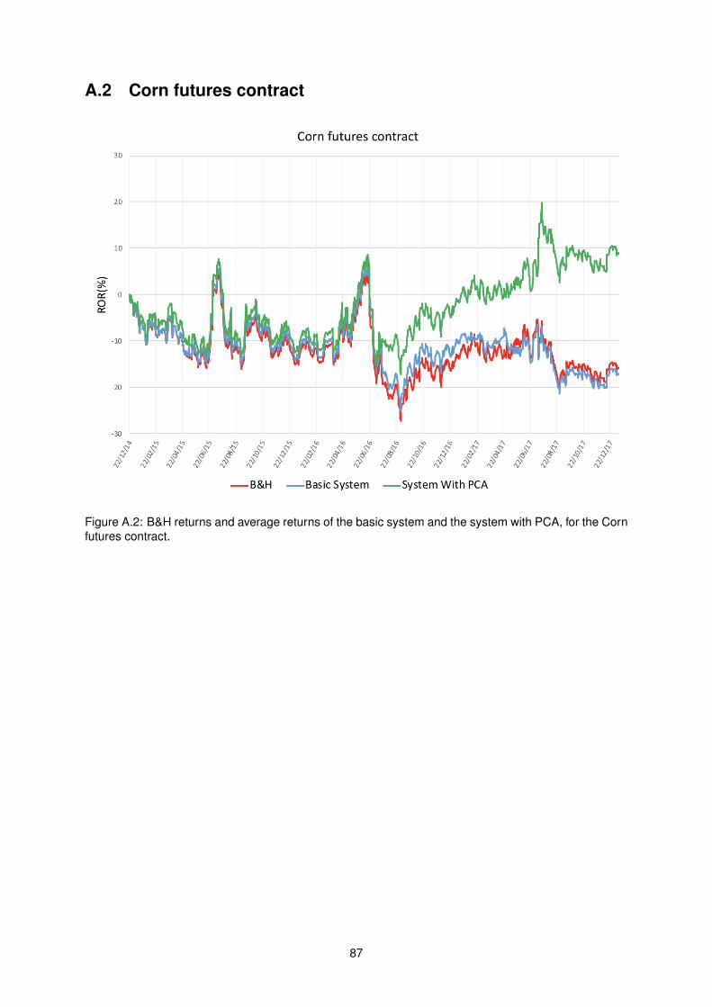
A.2 Corn futures contract
Figure A.2: B&H returns and average returns of the basic system and the system with PCA, for the Cornfutures contract.
87
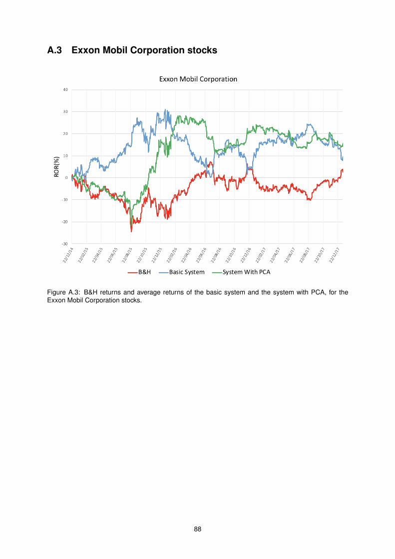
A.3 Exxon Mobil Corporation stocks
Figure A.3: B&H returns and average returns of the basic system and the system with PCA, for theExxon Mobil Corporation stocks.
88

A.4 Home Depot Inc. stocks
Figure A.4: B&H returns and average returns of the basic system and the system with PCA, for theHome Depot Inc. stocks.
89
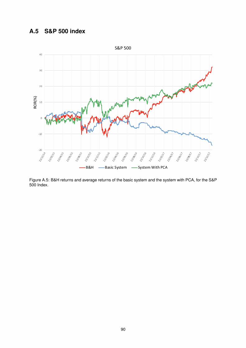
A.5 S&P 500 index
Figure A.5: B&H returns and average returns of the basic system and the system with PCA, for the S&P500 Index.
90

Appendix B
Return Plots of the Case Study II
B.1 Brent Crude futures contract
Figure B.1: B&H returns and average returns of the basic system and the system with Haar wavelet witha level of decomposition of 5, for the Brent Crude futures contract.
91

B.2 Corn futures contract
Figure B.2: B&H returns and average returns of the basic system and the system with Haar wavelet witha level of decomposition of 5, for the Corn futures contract.
92
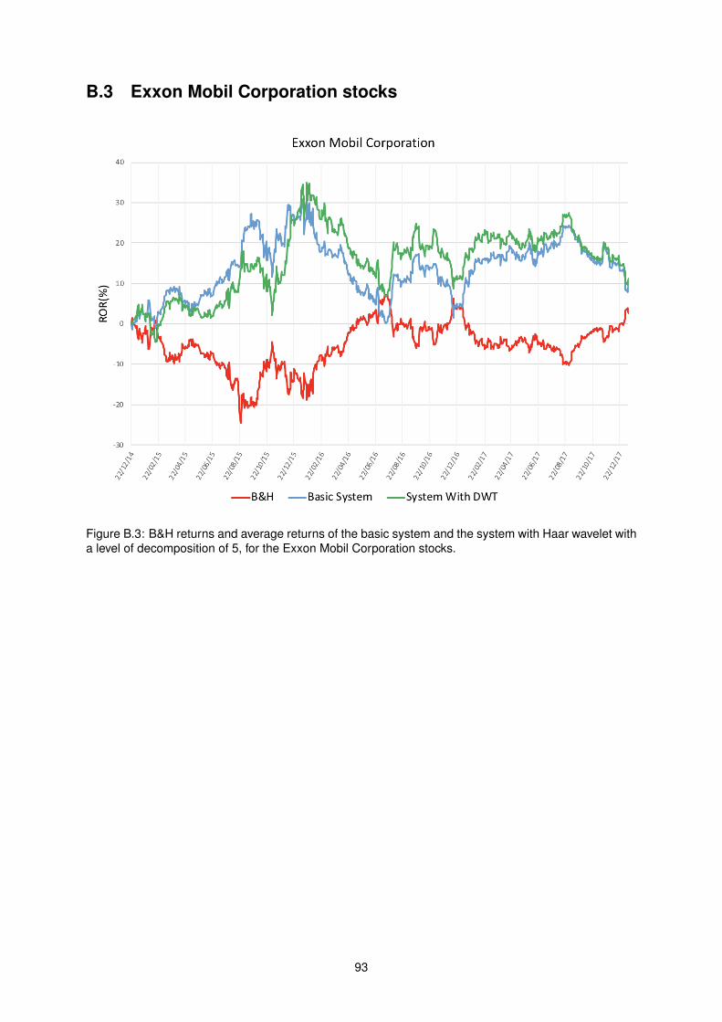
B.3 Exxon Mobil Corporation stocks
Figure B.3: B&H returns and average returns of the basic system and the system with Haar wavelet witha level of decomposition of 5, for the Exxon Mobil Corporation stocks.
93
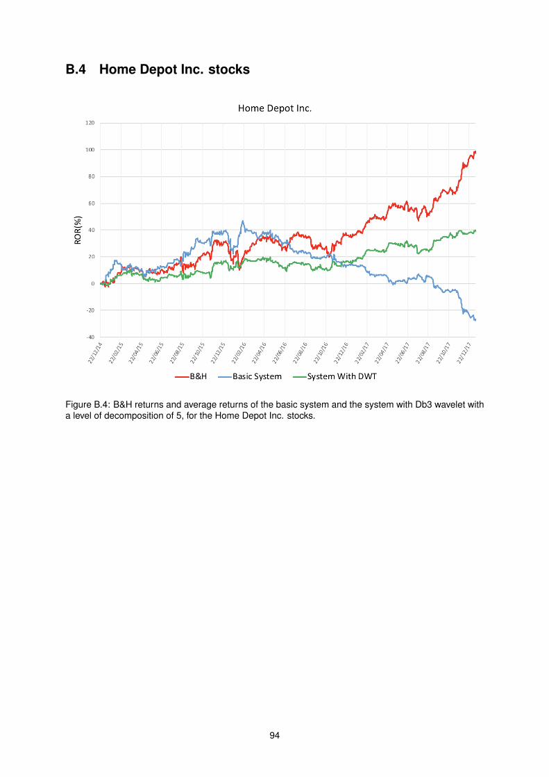
B.4 Home Depot Inc. stocks
Figure B.4: B&H returns and average returns of the basic system and the system with Db3 wavelet witha level of decomposition of 5, for the Home Depot Inc. stocks.
94

B.5 S&P 500 index
Figure B.5: B&H returns and average returns of the basic system and the system with Haar wavelet witha level of decomposition of 5, for the S&P 500 Index.
95