combining environmental fate and air quality...
TRANSCRIPT
Final Proceedings
Workshop on
Combining Environmental Fate and Air Quality Modeling
Organized by the Reactivity Research Working Group's
Atmospheric Availability and Environmental Fate Subgroup
June 27-29, 2000 Research Triangle Park, NC

1
FINANCIAL SUPPORT IS GRATEFULLY ACKNOWLEDGED FROM THE FOLLOWING ORGANIZATIONS
American Chemistry Council - Solvents Council American Chemistry Council - Atmospheric Chemistry Technical
Implementation Panel American Chemistry Council - Ethylene Glycol Ethers Panel American Chemistry Council - Propylene Glycol Ethers Panel Chemical Specialty Manufacturers Association Dunn-Edwards Corporation National Paint and Coatings Association Soap and Detergents Association
ORGANIZING COMMITTEE
Deborah Bennett Lawrence Berkeley Laboratory Don Fox University of North Carolina Doug Fratz Chemical Specialty Manufacturers Association Bob Hamilton Amway Corporation Bill Johnson U.S. Environmental Protection Agency Brian Keen Union Carbide Corporation Jon Kurland Union Carbide Corporation Sue Lewis American Chemistry Council Eileen McCauley California Air Resources Board Dave Morgott Eastman Kodak Company
The organizing committee would like to recognize the tireless efforts and thoughtful leadership offered by Jonathan Kurland during the preparation and planning of this workshop. The committee is also grateful to the U.S. Environmental Protection Agency for providing the meeting facilities and audiovisual equipment used by workshop attendees.
2
TABLE OF CONTENTS
Title Page Executive Summary ........................................................................................3 Overview........................................................................................................5 Background....................................................................................................6
Multimedia Urban Models...........................................................................6 Use of Fugacity-based Multimedia Models...................................................7 Air Quality Models and Component Modules ...............................................7 Environmental Fate of Indoor VOC Emissions .............................................8 Modeling of Chemical Transport in the Atmosphere .....................................9
Breakout Group Reports ...............................................................................10 Group 1...................................................................................................10 Group 2...................................................................................................12 Group 3...................................................................................................15 Discussion and Comments ......................................................................19 Consensus Summary....................................................................................20 Appendix A Workshop Program .................................................................24 Appendix B Workshop Presentations..........................................................28 Appendix C Key Topics List ......................................................................30
LIST OF FIGURES
Figure Page Figure 1. Multimedia Urban Model..................................................................7 Figure 2. Research Algorithm .....................................................................13 Figure 3. VOC Chemical Evaluation Diagram ...............................................17

3
EXECUTIVE SUMMARY This paper contains the proceedings from a workshop on Combining Environmental Fate and Air Quality Modeling that was organized by the Reactivity Research Working Group's subgroup on Atmospheric Availability and Environmental Fate. The workshop brought together experts in multimedia and air quality disciplines to establish prospects and priorities for the integration of environmental fate and air quality models. The goal of the workshop was to produce a set of research recommendations that would help in the development of a model for evaluating the importance of multimedia processes on the ozone forming potential of volatile chemicals. Forty experts from a variety of disciplines including multimedia modeling, air quality modeling, indoor air quality, and dispersion modeling participated in the workshop, which was held on June 27-29, 2000 at the EPA Administration Building in Research Triangle Park, NC (Appendix A). On the first day of the meeting, experts representing the above disciplines gave background presentations to introduce participants to important concepts in these fields (Appendix B). On the second day, participants were divided into three working groups and asked to consider the following:
?? Determine the importance of transport to and from water soil, sediment, and other media and of transformation in these media on the ozone forming potential of different VOC capable of contributing to tropospheric ozone and particulate matter (PM2.5).
?? Identify environmental fate processes that significantly influence the concentration of VOC in the atmosphere.
?? Investigate mechanisms to address the integration of fate and transportation into air quality models.
?? Propose priorities for the integration of environmental fate and air quality models.
These topics are further outlined and expanded in Appendix C. Each working group contained experts from several disciplines. Participants reconvened on the third day of the meeting and a representative from each group presented their recommendations. The results from these presentations were used to establish future research priorities. A staged research plan was developed to assess the importance of atmospheric availability on the ozone formation potential of VOCs.
1. Survey candidate chemicals using environmental fate models to determine the range of compounds whose ozone-forming potential is affected by partitioning.
2. Develop an initial screening box model that combines an air quality model and environmental fate (multimedia) model.

4
3. Use the screening model to compare the results of environmental fate models and the screening air quality/environmental fate model with regard to the fraction of various VOC oxidized in air.
4. Continue with the development of a grid model capable of being used for regulatory purposes, if environmental fate is found to have an appreciable effect on the ozone forming potential of important VOCs.
Somewhat lower priorities were later established by the Reactivity Research Working Group for the following research.
1. Consider the environmental fate of indoor emissions, indoor sinks and sources.
2. Consider the environmental fate of photochemical oxidation products and their impact on the estimation of the ozone-forming potential of VOCs (e.g., MIR values).
The workshop was successful in bringing together experts from a variety of disciplines to discuss the impact of multimedia processes on the ozone forming potential of VOCs. There was a useful exchange of information and ideas among workshop participants. The recommendations will help focus future research, leading to the development of a model that can evaluate the importance of multimedia processes on the formation of ozone by VOCs capable of contributing to tropospheric ozone.
5
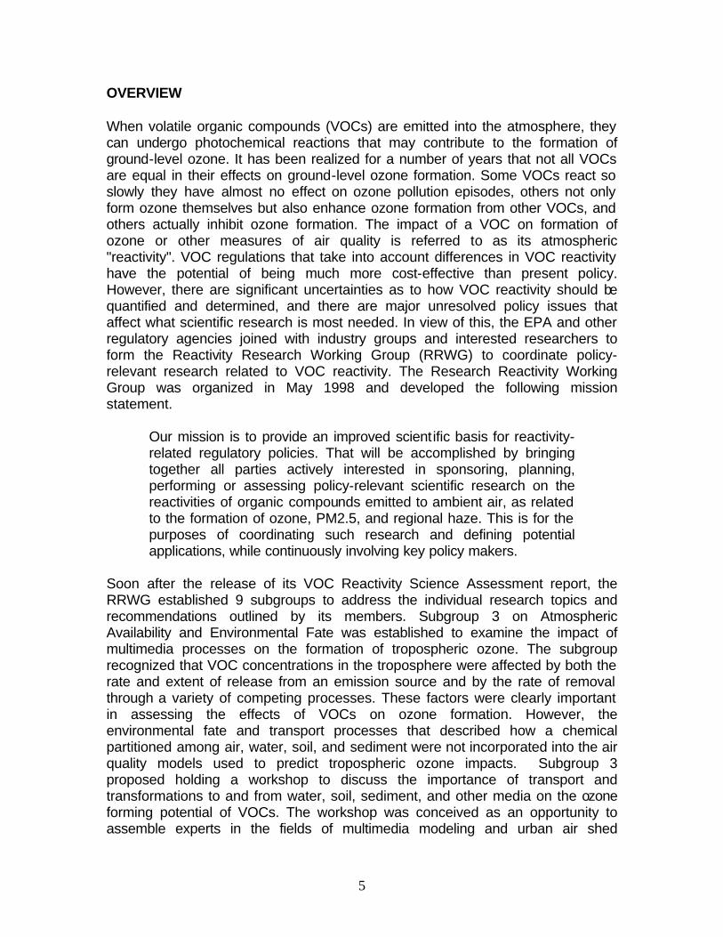
OVERVIEW When volatile organic compounds (VOCs) are emitted into the atmosphere, they can undergo photochemical reactions that may contribute to the formation of ground-level ozone. It has been realized for a number of years that not all VOCs are equal in their effects on ground-level ozone formation. Some VOCs react so slowly they have almost no effect on ozone pollution episodes, others not only form ozone themselves but also enhance ozone formation from other VOCs, and others actually inhibit ozone formation. The impact of a VOC on formation of ozone or other measures of air quality is referred to as its atmospheric "reactivity". VOC regulations that take into account differences in VOC reactivity have the potential of being much more cost-effective than present policy. However, there are significant uncertainties as to how VOC reactivity should be quantified and determined, and there are major unresolved policy issues that affect what scientific research is most needed. In view of this, the EPA and other regulatory agencies joined with industry groups and interested researchers to form the Reactivity Research Working Group (RRWG) to coordinate policy-relevant research related to VOC reactivity. The Research Reactivity Working Group was organized in May 1998 and developed the following mission statement.
Our mission is to provide an improved scientific basis for reactivity-related regulatory policies. That will be accomplished by bringing together all parties actively interested in sponsoring, planning, performing or assessing policy-relevant scientific research on the reactivities of organic compounds emitted to ambient air, as related to the formation of ozone, PM2.5, and regional haze. This is for the purposes of coordinating such research and defining potential applications, while continuously involving key policy makers.
Soon after the release of its VOC Reactivity Science Assessment report, the RRWG established 9 subgroups to address the individual research topics and recommendations outlined by its members. Subgroup 3 on Atmospheric Availability and Environmental Fate was established to examine the impact of multimedia processes on the formation of tropospheric ozone. The subgroup recognized that VOC concentrations in the troposphere were affected by both the rate and extent of release from an emission source and by the rate of removal through a variety of competing processes. These factors were clearly important in assessing the effects of VOCs on ozone formation. However, the environmental fate and transport processes that described how a chemical partitioned among air, water, soil, and sediment were not incorporated into the air quality models used to predict tropospheric ozone impacts. Subgroup 3 proposed holding a workshop to discuss the importance of transport and transformations to and from water, soil, sediment, and other media on the ozone forming potential of VOCs. The workshop was conceived as an opportunity to assemble experts in the fields of multimedia modeling and urban air shed

6
modeling to consider the possibility of including multimedia processes in air quality models and propose new research on the topic.
The underlying hypothesis for the workshop was that atmospheric availability might be as important to the formation of tropospheric ozone as reactivity in the gaseous phase. This hypothesis resulted in workshop discussions concerning the overall impact of multimedia modeling predictions on atmospheric reactivity, the significance of environmental fate modeling on the formation of ozone, and the manner in which any changes in ozone formation are manifested.
BACKGROUND The objectives of the workshop were: 1) to produce research recommendations that would help in the development of a model which can evaluate the importance of multimedia processes on the ozone-forming potential of compounds; and 2) to establish prospects and research priorities for the integration of environmental fate and air quality models. The following questions served to guide many of the group discussions:
?? Do air quality and multimedia models need to be linked at a screening level for assessing the impact of different multimedia compartments?
?? Is it feasible to link Level IV, time-dependent multimedia models with photochemical box models?
?? Can a model integration scheme will provide a framework for directing needed research on compartmental chemistry and mass transfer rates?
?? Can a research paradigm be identified that provides a progressive, systematic approach for directing the development and evolution of an air quality model that incorporates all relevant multimedia processes?
Summaries of the talks that were presented at the start of the workshop to provide background information on each of the related fields follow. Multimedia Urban Models (Miriam Diamond) The speaker has conducted numerous studies on the importance of multimedia partitioning in the urban environment. This work was highlighted to help workshop participants better understand the fate of compounds in the environment. She has conducted research on the importance of various surface films in the urban environment. Figure 1 depicts an urban multimedia model containing a film compartment that she has developed. Chemicals have only a short residence time in the films, but the films can be a means of sweeping compounds out of the air and into the water instead of depositing directly onto vegetation or in the soil.

7
Figure 1. Multimedia Urban Model Use of Fugacity-based Multimedia Models to Assess the Fate of Chemicals in the Environment (Charles Staples) This presentation on fugacity based multimedia models summarized how these models are set up and designed. An example showed how the mass balance for air includes transfers to and from soil and water, sources to the air, advection losses out of the model region, and transformation processes. To model a chemical, information is needed on the partition coefficients and degradation rates in multiple environmental media. The speaker also presented an example of the steady-state distribution of isobutanol, a chemical intermediate commonly used as a solvent. When emitted to air, 80% is found in the water, 14% in the soil, and 6% in the soil, thus for this chemical, the entire mass in not available for reactions in the atmosphere. Air Quality Models and Component Modules (Gail Tonneson) This presentation was a “background” talk on air quality modeling designed for a mixed audience of scientists and regulators in the fields of air quality modeling and multimedia modeling. The purpose of this talk was to provide sufficient background on scientific and data aspects of air quality modeling so that an interdisciplinary team of scientists could discuss approaches for integrated, multi-media modeling of low volatility compounds, including their fate and their possible contribution to air pollution. Key topics addressed include the following: types of air quality models, including dispersion models, simple box modes,
AIR FILM VEGETATION
WATER
SEDIMENT
SOIL

8
trajectory models, and gridded, regional scale air quality models; necessary inputs for air quality models, including meteorological fields, emissions inventories, and photochemical mechanisms; auxiliary models and preprocessors required for generating air quality model inputs; introduction to the photochemistry of gas phase and heterogeneous chemistry and aerosol formation; key uncertainties in model inputs and formulation; and approaches for model evaluation and validation. While there are large uncertainties in model inputs and in the accuracy of models in forecasting future conditions, model predictions of concentrations of the hydroxyl radicals (OH) and ozone (O3) are relatively insensitive to these uncertainties and are useful for examining the fate of low volatility VOC. The aerosol formation mechanisms represented in regional scale air quality models are still somewhat primitive, particularly for the formation of secondary organic aerosols (SOA) from low volatility VOC. Improved SOA formation mechanisms is a key area requiring improvement for determining the fate and impacts of low volatility VOC. Relatively simple trajectory models, for example the OZIP/EKMA trajectory model, may be useful as a screening tool and a first step in linking multi-media models with photochemical air quality models. Environmental Fate of Indoor VOC Emissions: The Role of Indoor Chemistry (Jim Zhang) Another of the background presentations addressed the environmental fate of VOC’s that are emitted in buildings, including houses, apartments, public buildings and commercial buildings. In addition to providing a list of some VOC’s that might be emitted indoors, Dr. Zhang described alternate fates of those VOC’s that might preclude emission to outdoor air. The particular emissions and typically higher concentration of indoor air pollutants demands some careful review of the reaction chemistry that might occur both in indoor air and on indoor surfaces. These reactions are constrained by shorter time frames, related to air exchange rates with outdoor air, than those of typical multimedia modeling. Still some of the surface chemistry and radical induced formation of particulates and semi-volatile condensation products give indication that indoor emissions may not simply migrate unchanged to the outdoor atmosphere. The speaker concluded that indoor environments are often not passive boxes for VOC emissions. Also, indoor air chemistry is complex and not well appreciated at present. The surface to volume ratio in indoor environments is quite high so adsorption, absorption, and surface chemistry are more important indoors. Indoor environments also are more carefully controlled for temperature, light energy and humidity and may thus be more predictable regarding physical chemical characteristics. Finally, human activities can have a greater impact on air emissions indoors than on outdoor emissions; therefore, it may be an appropriate experimental environment for further study.

9
Modeling of Chemical Transport in the Atmosphere (Christian Seigneur) The processes that govern the transport of chemicals in the atmosphere were described in this presentation. Atmospheric transport processes include emissions, plume rise, advection and convection, turbulent dispersion, gas/particle partitioning, dry deposition and wet deposition. Trajectory (Lagrangian) models for chemical transport follow a parcel of air as it travels away from a source. Fixed-grid (Eulerian) models deal with emissions, chemistry and depositions within grid cell. Trajectory models are best suited for stack plumes, but are computationally expensive for multiple reactive plumes. Fixed grid models are best suited for areas with multiple sources and reactive species. Plume models can be imbedded into grids for better treatment of stack plumes. Partitioning of semi-volatile compounds between the gas phase and particle phase is a function of the thermodynamic properties of the compound, temperature, relative humidity and atmospheric particulate matter. Adsorption or absorption may occur, and they are modeled as functions of the supercooled liquid vapor pressure and the octanol/air partition coefficient respectively. Absorption of hydrophilic compounds on particles with an aqueous phase is governed by Henry’s law. Most air quality models assume one-way irreversible dry deposition by gravitational settling and turbulent transport against resistances such as aerodynamic resistance. For some compounds atmosphere/surface equilibrium is assumed (no net transfer). Wet deposition is removal by precipitation dissolved in water droplets. It is called rainout if it occurs in-cloud and washout if below-cloud. It is especially important if solubility in water is enhanced by chemical reactions in the aqueous phase, e.g., ammonium sulfate formation from ammonia in aqueous sulfuric acid. In air quality models dry and wet deposition of soluble organic compounds (aldehydes, alcohols, acids) is calculated, but deposition of organic compounds of low solubility is generally neglected.

10
BREAKOUT GROUP REPORTS Group 1 Rapporteurs:
Don Fox University of North Carolina Brian Keen Union Carbide Corporation
Participants: Roger Atkinson University of California, Riverside Deborah Bennett Lawrence Berkeley Laboratory Frank Binkowski U.S. Environmental Protection Agency Manuel Cano Equilon Enterprises LLC Donald Dabdub University of California, Irvine Miriam Diamond University of Toronto David Guinnup U.S. Environmental Protection Agency Harvey Jeffries University of North Carolina Paul Makar Environment Canada Jim Neece Texas Natural Resources Conservation Committee Jay Olaguer The Dow Chemical Company Bill Stockwell Desert Research Institute Jim Zhang Rutgers University
Group 1 concluded that the first priority for further research is a screening level assessment to estimate the effect of multimedia partitioning on the atmospheric availability of a wide range of chemicals. This is a relatively easy task that could be accomplished in conjunction with other projects. The following factors were deemed to be important considerations in the study design:
?? A variety of compounds covering a wide range of physical and chemical properties should be included in the screening assessment. The screening assessment should focus on primary emissions (i.e., compounds that are emitted directly to the environment) and secondary photooxidation products that can participate in ozone formation.
?? A Level Ill or greater multimedia model needs to be used in the screening assessment. A Level Ill model would provide a steady-state simulation that could cover a wide variety of environmental conditions.
?? Emissions to a variety of environmental compartments, notably air, water, and soil, should be included in the model simulations. Also, the assessment should consider a variety of different environmental conditions (e.g., amount of vegetation, different meteorological conditions, and different temperatures).
After completing a screening level assessment on a wide variety of compounds, researchers will need to evaluate the results and determine if multimedia partitioning affected the availability of a sufficient number of chemicals to merit a more detailed assessment. Criteria will need to be established for judging whether work should proceed to the next step. For instance, researchers will

11
need to assess whether the impacted chemicals are used in sufficient quantities to be of practical scientific concern and whether the chemicals are relevant to atmospheric reactivity. Once a list of compounds has been identified for further investigation, researchers will need to develop a linked air quality/multimedia model for further in-depth analysis. The comprehensive model can be developed by either attaching an air quality model to a multimedia model or by incorporating a multimedia model into an existing air quality model. Once an approach has been decided upon, it will be important to establish compatibility requirements for the assembled model (e.g., the spatial and temporal scales will need to be explored along with the nature of the model linkage). The comprehensive model should be used to assess the fate of the target compounds that satisfied the experimental criteria developed following the screening assessment. Model performance needs to be evaluated by calibrating and testing the results against actual ambient data. A data collection program should be designed that will facilitate model validation. This program would include the:
?? selection of a range of test chemicals; ?? selection of a range of test conditions and environmental characteristics; ?? identification and collection of existing data sets; ?? integration of data needs with existing data collection programs, such as
the EPA Supersites Program; ?? use of multimedia sampling methods that could simultaneously examine
chemicals in air, water, sediment, vegetation, soil and organic films.
The uncertainty, variability, and sensitivity of model results need to be calculated. This is an important step that will establish confidence in the results and promote the model as a useful predictive tool. The following criteria were identified to aid in the test chemical selection process.
?? The compounds should have a wide range of physical and chemical properties that are relatively well known.
?? The source emissions of these compounds should be reasonably well known.
?? Analytical methods should be available to measure concentrations in a variety of environmental media (i.e., above the detection limit).
?? The compounds should be relatively abundant in the environment so that ambient concentrations can be accurately assessed.
?? The compounds should cover a range of partitioning behavior such that they are found in a range of environmental compartments.
?? The compounds need to be relevant to atmospheric reactivity and encompass important reaction mechanisms.

12
Group 2 Rapporteurs:
Eileen McCauley California Air Resources Board Dave Morgott Eastman Kodak Company
Participants: Dan Baker Equilon Enterprises LLC John Chang U.S. Environmental Protection Agency Joyce Graff Cosmetic Toiletry & Fragrance Association Bill Johnson U.S. Environmental Protection Agency Richard Kamens University of North Carolina John Little Virginia Polytechnic Institute Tom McKone University of California, Berkeley Mehran Monabbati SENES Consultants Limited Dennis Peterson ExxonMobil Jon Pleim National Oceanic & Atmospheric Administration/U.S. EPA Christian Seigneur Atmospheric Environmental Research Gail Tonneson University of California, Riverside
The discussions within group 2 were organized around two previously stated workshop objectives:
1. to produce research recommendations that will help in the development of a model which can evaluate the importance of multimedia processes on the ozone-forming potential of compounds, and
2. to establish prospects and research priorities for the integration of environmental fate and air quality models.
The group felt that it was currently feasible to combine a Level IV multimedia model with a photochemical box model to identify the impact of different multimedia compartments on ozone formation. This direct approach involving model construction before chemical evaluation was felt to be necessary in order to accurately assess the importance of different environmental processes within the context of an air-shed model. The group believed that the outlined model integration scheme provided a framework for directing other research on compartmental chemistry and mass transfer kinetics. The suggested research paradigm also provided a progressive, systematic approach for linking air quality and multimedia models at an initial screening level. This will aid in the development and evolution of a more sophisticated air quality model that could incorporate all relevant multimedia processes. The initial combination of a Level IV multimedia model with a photochemical box model would provide the screening model to be used for the chemical assessment. The output from this model would help identify the chemical and kinetic research needed for modeling important physical and chemical processes. The group noted that inorganic nitrogen containing compounds and VOCs should both be studied using the screening model. If multimedia effects

13
were found to have a significant impact on ozone formation, researchers would then move to develop a more sophisticated grid model. The scheme outlined in Figure 2 summarizes the model development process. Figure 2. Research algorithm Phase I
?? Initial box model construction ?? Sensitivity analysis
Phase II ?? Add chemical complexity and kinetics ?? Expand to grid model
When constructing the box model, all multimedia compartments should be included. For example, indoor surfaces should be included as both an emissions source and sink if possible. The group suggested using a photochemical box model that can describe aerosol formation and partitioning. Finally, model sensitivity will need to be evaluated using chemicals with a range of vapor pressures, octanol/water partition coefficients, and chemical properties. If multimedia partitioning is shown to have some effect on ozone formation, researchers will need more information on the chemistry and chemical reactions that occur in the different compartments. The group recommended the following steps for collecting this information:
?? Review all pertinent literature on the chemical reactions that apply to each compartment in the model (e.g., surface water, soil, vegetation, surface films, sediment, etc.).
?? Obtain reasonable estimates of the compartmental chemistry when data is unavailable (include nitrogen chemistry).
Develop Screening Box Model
Investigate Chemistry & Mass Transfer
Kinetics
Develop Grid Model

14
?? Improve estimates of mass transfer kinetics and emissions rates for chemicals and processes of interest.
Stage I of the suggested research plan would include model construction and a sensitivity analysis using range of chemical properties. The following goals were specifically identified for Stage I research:
?? Determine the most important compartments needing representation in the model.
?? Determine the chemical classes most affected by compartmental partitioning.
?? Determine the physical chemical properties that exert the most influence on the VOC that are sensitive to multimedia partitioning.
?? Determine the future data needs for grid model development.

15
Group 3 Rapporteurs:
Doug Fratz Chemical Specialties Manufacturers Association Bob Hamilton Amway Corporation
Participants: Daewon Byun National Oceanic & Atmospheric Administration/U.S. EPA Bill Carter University of California, Riverside Nick Hazel BP Amoco Europe Ajith Kaduwala California Air Resources Board Dave McCready Union Carbide Corporation Stephen McDow Drexel University Randy Maddalena Lawrence Berkeley Laboratory Glenn Morrison National Oceanic Atmospheric Administration Ted Russell Georgia Institute of Technology Martin Scheringer ETH Zurich Charles Staples Assessment Technologies
Group 3 independently examined the two main areas of impact for multimedia modeling: 1) the effect of alternate environmental fates on the VOC inventory used in atmospheric photochemical modeling and 2) the possible multimedia impacts on the photochemical process model. These were deemed to be the most important impacts of integrating multimedia events into air quality models. If multimedia modeling indicates that VOC emissions are partitioning into other compartments in the environment, the air emissions inventory would need to be correspondingly adjusted. The group agreed that the ultimate fate of these partitioned materials must be monitored. If partitioning is time dependent as expected by the multimedia model, which assumes extended equilibrium time frames, the re-emission of volatile organics or of reaction products must be considered. The temporary storage of reactive species may result in net neutral or negative impact on ozone formation. This is especially important if peak ozone concentrations in air are considered the basis for regulatory limits. Likewise, the multimedia modeling could have a variety of effects on the photochemistry process. If multimedia processes selectively remove VOC species, the photochemistry of the local atmosphere may be significantly altered. Therefore, the input parameters for to the air quality model would need to be modified to reflect changing equilibria resulting from differing available species concentrations. The group also discussed several important ancillary issues. These included topics such as model fit and the effects of multimedia processes on air shed model uncertainty and predictive ability. Another issue concerned the differences in time scale between air quality models, which dynamically look at ozone limit

16
exceedence events that can be 1-3 days in length, and multimedia models which are very large static box models in a state of equilibrium. Other important considerations included:
?? Local impacts ? what are the rates of equilibration and points of emissions?
?? Regional ozone levels ? do multimedia models help to better understand regional transport or background of ozone levels?
?? Regulatory policy ? should multimedia models be important in the development of a regulatory policy even though there may not be a significant impact on ozone formation?
In order to address these issues, a tiered approach was used to develop research recommendations. The following topics were examined independently in conjunction with the test plan design. Emissions inventory issues:
?? Emissions profile ? what are the impacts of having VOCs emitted in different multimedia compartments?
?? Environmental fate ? what, if any, are the alternate fates for these compounds? If the compounds are simply re-emitted to the air, is there any net effect? Clearly, if the compounds are removed (e.g. by biodegradation), there will be and impact on photochemical reactions.
Photochemical modeling issues: ?? Direct deposition ? if multimedia modeling demonstrated deposition to
surfaces, then we could determine if this is important for certain VOCs. ?? Aerosol formation ? this issue includes condensation and adsorption onto
existing aerosols. Are aerosols accounted for in local ozone production? ?? Heterogeneous reactions ? multimedia considerations may involve media
surfaces or certain reactions that can have a positive or negative impact on heterogeneous reactions.
The plan depicted in Figure 3 was developed for the identification of compounds to be used in a screening level model. Because of the expenditures needed for the integration of multimedia and air quality models, the discussion focused on a screening process that used existing multimedia and air quality models. The group noted that it would be important to concentrate on VOC species that were important in the regulatory process.

17
Figure 3. VOC Chemical Evaluation Diagram A = Multimedia partitioning significant for VOC emissions B = Air quality modeling demonstrates shows deposition is significant relative tofor ozone formation VOC species that are substantially affected by multimedia compartmentalization would be included in circle A. VOC species that are highly active inwhere deposition could affect photochemical reactivity modelsthe amount of ozone they produce would be included in circle B. The intersection of the two circles would form the VOC category from which candidates should be selected for further study since they would have maximum multi-media impact on ozone formation in each model. The group indicated that a focus on episodic emissions could help to determine whether multimedia processes had an impact on the formation of ozone. One area of particular interest was indoor (household) multimedia fates. These may be important because households provide a lot of opportunity for partitioning and could lead to longer VOC retention times. Some examples of alternative fates included:
?? Down-the-drain events where compounds get mixed into waste water leaving the home.
?? Solid waste adsorption where VOCs are deposited on particles before clean-up and disposal in the garbage.
?? The consumption of compounds by combustion. ?? Temperature control and the large variety of surface types that could be
important for low vapor pressure chemicals.
Multimedia Model 3D
Air Quality Model
A B
A ? B
Run in parallel
Better data on fate Better inventory
data
Integrated Model
Physical & Chemical Properties
VOC Species VOC Species

18
?? Biological degradation by insects, fungi, or bacteria. ?? Transformation processes that can convert a chemical to a more complex
material that is not emitted or to a VOC with a different ozone forming potential.
Another important episodic event that may be impacted significantly by multimedia partitioning is emissions from industrial processes. These are usually in confined areas that may or may not involve some type of VOC control. These types of scenarios would need to be studied on a case-by-case basis. Additional processes may also need to be considered. For example, paint solvents trapped in and under the film coating may function as a sink process. Mixing two ingredients with disparate volatilities could reduce the overall vapor pressure and retard the evaporation of the more volatile ingredient. As with industrial process emissions, reactive transformations are a special case and would need to be studied individually. The group also addressed several general effects that could impact the emissions inventory. They included: washout via rain, fog, and clouds, and entrainment or reemission of a chemical following a spill on an absorbent surface. The effects of washout would be expected to be minimal on locally generated ozone, but could have an impact on downwind areas. A brief overview was given of a Canadian Modeling Center urban case study that showed how a simple multimedia model could be used in screening level assessment. The objective was to demonstrate the types of information that could be gained to see how multimedia might impact photochemistry models. The study looked at how other media impacted the amount of chemical available in the atmosphere for reactions which lead to ozone formation. Multimedia events could affect photochemical modeling in three different areas:
1. Direct deposition ?? removal by biological and chemical degradation ?? removal by advection or fluid flow following deposition on a stream or
lake 2. Aerosol Formation
?? removal by advection may take compound out of local box but may place it downwind for reaction.
?? removal by deposition 3. Heterogeneous Chemistry
The following list of research recommendations was ultimately developed and submitted for consideration by the group: 1) Multimedia screening analysis
?? hypothetical mapping of: ??boundary conditions ??physiochemical properties ??sensitivity
?? photochemical model screen

19
?? maximization of the deposition factor 2) Determination of the relative loss to alternative fates 3) Test the sensitivity to multimedia landscape variation (Emphasis on urban) 4) Screen for sensitivity to the aerosol formation factor 5) Prioritize indoor air emissions 6) Rain/fog/cloud disposition effects screen (with Level IV model) 7) Study of possible sink effects 8) Harmonization of different model types
?? validity ?? uncertainty ?? utility
DISCUSSION AND COMMENTS Tom McKone suggested using a Monte Carlo approach for selecting chemical properties for test runs rather than making test runs on a number of compounds. He noted that by using this approach, one could define the range of desired physical/chemical properties. Eileen McCauley added that the workgroup is interested in ozone formation. If the compounds do not have an impact on ozone concentration, then they are not of interest to the RRWG. Tom McKone noted that in the initial model there would be no spatial resolution since only a single grid cell would be used. Miriam Diamond suggested that we need to test a wide range of environmental conditions in the model runs. Eileen McCauley agreed and noted that we would certainly expect different results from Toronto and Los Angeles. Sue Lewis asked if people are considered sinks. Tom McKone responded that people could be considered sinks. For example, dry cleaning workers are sinks for perchloroethylene and farm workers are sinks for certain pesticides. Bill Carter indicated noted that one point that was not brought up is the potential mechanisms for absorption onto surfaces. Also, when the temperature goes up, ozone formation increases. Brian Keen noted that all surfaces are not created equal. Dave Guinnup added that we need to be careful when adjusting emissions inventories for ozone forming potential. It needs to be done in such a way that we know that the adjustments have been made.

20
Doug Fratz said there are a number of compartments we need to look into, including water, indoor air, and outdoor air. There could be permanent sinks that we need to evaluate. Transport could impact air quality models because it could take VOCs out of the region. A question that the group could not answer is of the surface amounts in an urban air shed during a nonattainment episode, what percent of surfaces are suspended versus stationary? Don Fox asked for comment on how photochemical models look at partitioning between gas and particle phase. Gary Whitten said one type of methodology not discussed would be parameterization of nitrous acid. You could use this with multimedia grid model to assess validity. Robert Wendoll noted that one of the issues that came up repeatedly in Group 1 was the need to better account for secondary products of primary emissions. These products may have very different physical and chemical properties that make them more or less susceptible to multimedia partitioning. Brian Keen stated that we need to investigate biogenic emissions during screening. We need to understand the fate of these emissions, as well as how some of these compounds impact the removal of other compounds. Robert Hamilton indicted that indoor air provides a relatively good controlled environment that can be used to investigate the impact of multimedia processes. CONSENSUS SUMMARY The underlying hypothesis for the workshop was that atmospheric availability might be as important to the formation of tropospheric ozone as reactivity in the gaseous phase. This hypothesis resulted in workshop discussions concerning the overall impact of multimedia modeling predictions on atmospheric reactivity, the significance of environmental fate modeling on the formation of ozone, and the manner in which any changes in ozone formation are manifested. To address the first question an environmental fate process model must be constructed. This model consists of a coupled set of environmental compartments that exchange mass as shown in Figure 1. If compounds at equilibrium are entirely in the air compartment, then there is no multimedia impact on the air quality model. It is very important to obtain as much information as possible regarding chemistry and rate studies for input to the models. This begins by reviewing all pertinent literature on the chemical reactions that apply to each compartment in the model (surface water, soil, vegetation, surface films, sediment, etc.). If data are unavailable, reasonable estimates of compartmental chemistry (including nitrogen chemistry) must be obtained. It is important to

21
improve estimates of mass transfer and emissions rates for chemicals and processes of interest. Multimedia modeling has been used mainly in the study of persistent organic pollutants (POPs). Recently it has been extended to shorter times and smaller areas, including urban areas and to include such compartments as urban films. Films can be important as a means of sweeping compounds out of the air Into water instead of depositing directly onto vegetation or in the soil. The second question relating to the hypothesis is what is the impact or significance of environmental fate in the formation of ozone. Multimedia processes may play a role in two places - in the emissions inventory and in the photochemical modeling. It is important that the emissions inventory provide the best possible information as to the actual emissions to the atmosphere. For some compounds, multimedia processes may result in a decreased fraction of emissions actually present in the air. There must be losses between the compartments for there to be a multimedia impact on the air quality model. Multimedia processes may also need to be considered in photochemical models. Partitioning of intermediate chemical species into other media including aerosols and transformation in the particle phase into compounds which are then remitted are only two of many possible processes which may have an effect on ozone formation. It is also important in the photochemical model to identify any products of oxidation that are important in the formation of ozone. If these secondary products disappear or are not available for reaction, then the model runs are inaccurate. The workshop members suggested that investigation of the importance of multimedia processes on ozone formation begins with the development of an initial screening box model. In the development of the initial screening box model it is important to include all multimedia compartments. In addition, the indoor environment must be included as an emissions source and sink. The photochemical box model that is selected for use must describe aerosol formation and partitioning. Finally, model sensitivity must be analyzed using chemicals with a range of vapor pressures, octanol/water partition coefficients, and chemical properties. After performing a sensitivity analysis, chemistry and mass transfer rates are added to the model. If environmental fate is found to be important, the process continues with the development of a grid model. Finally, it is important to identify where to get the best fit between the two kinds of mode. This is because multimedia and air quality models work with different grid sizes and use different timeframes. For example, local impacts usually have a small grid and short time frame and are further from correct equilibrium approximations than regional scale impacts. The following four questions were chosen to direct the first stage of research into combining environmental fate and air quality models:

22
?? What are the most important compartments needing representation in the model?
?? Which chemical classes are most affected by compartmental partitioning? ?? What physical/chemical properties are important in assessing which VOCs
are most affected by multimedia processes? ?? What are the future data needs for grid model development?
A staged research plan was developed to assess the importance of atmospheric availability on the ozone formation potential of VOCs. 1. Survey candidate chemicals with environmental fate models to see the range
of compounds whose ozone-forming potential is possibly affected. The focus is on correcting emissions inventories. If there is no multimedia effect in terms of the emissions inventory, there is no need to combine the multimedia with the air quality models. Which chemical classes are most affected by compartmental partitioning? What physical/chemical properties are important in assessing which VOCs are most affected by multimedia processes?
2. Model development begins with the development of an initial screening box
model that combines an air quality model and environmental fate (multimedia) model. In the development of the model it is important to include all multimedia compartments. The photochemical box model that is selected for use must describe aerosol formation and partitioning. What physical/chemical properties are important in assessing which VOCs are most affected by multimedia processes? Sensitivity analysis will provide a framework for directing needed research on compartmental chemistry and mass transfer rates.
3. Use the screening model to compare the results of environmental fate models
and the screening air quality/environmental fate model with regard to the fraction of various VOC oxidized in air. What are the most important compartments needing representation in the model? Which chemical classes are most affected by compartmental partitioning? If compounds are in equilibrium between the various compartments, then there is no multimedia impact on the air quality model. There must be losses between the compartments for there to be a multimedia impact on the air quality model. Finally, model sensitivity must be analyzed using chemicals with a range of vapor pressures, octanol/water partition coefficients, and chemical properties.
4. If environmental fate is found to be important, the process continues with the
development of a grid model capable of use for regulatory purposes. The suggested research paradigm provides a progressive, systematic approach for directing the development and evolution of an air quality model that incorporates all relevant multimedia processes. What are the future data needs for grid model development? Finally, it is important to identify where to get the best fit between the two kinds of model. This is because multimedia

23
and air quality models work with different grid sizes and use different time frames there is a natural clashing between the models. For example, local impacts usually have a small grid and short time frame and are further from correct equilibrium approximations than regional scale impacts.
Somewhat lower priorities were later established by the RRWG for the following research. 1. Consideration of the environmental fate of indoor emissions, indoor sinks and
sources. These may be unimportant relative to other sources, but they are important to regulating products, particularly consumer products and household paint, that are used extensively indoors.
2. Consideration of the environmental fate of products of photochemical
oxidation and its impact on estimations of the ozone-forming potential of VOC (e.g., MIR values). If these secondary products are transported to other compartments before they react in air are then consumed, then the model predictions are inaccurate.

24
APPENDIX A
Workshop Program

25
Workshop on Combining Environmental Fate and Air Quality Modeling
Sponsored by the Reactivity Research Working Group
Subgroup 3 on Atmospheric Availability and Environmental Fate
The Reactivity Research Working Group (RRWG) was organized in May 1998 to bring together people from the EPA Offices of Research and Development and Air Quality Planning and Standards, industry, and the scientific community. The mission of the RRWG is to “…provide an improved scientific basis for reactivity-related regulatory policies”. This will be accomplished by bringing together all parties actively interested in sponsoring, planning, performing or assessing policy-relevant scientific research on the reactivities of organic compounds emitted to ambient air, as related to the formation of ozone, PM2.5, and regional haze. The RRWG seeks to coordinate such research and define potential applications, while continuously involving key policymakers.” The RRWG is affiliated with NARSTO. Background Preliminary work indicates that multimedia processes may have an affect on the ozone forming ability of some volatile organic compounds (VOCs). The RRWG selected this topic as worthy of investigation. A working group has been formed to develop research priorities. At an initial meeting, the group defined their goal as helping to determine the importance of transport and transformations to and from water, soil, sediment, and other media on the ozone forming potential of different VOCs capable of contributing to tropospheric ozone. Purpose of the Workshop To bring together experts in the fields of both air quality modeling and multimedia modeling to establish prospects and priorities for integration of environmental fate and air quality models. The goal is to produce research recommendations that will help in the development of a model which can evaluate the importance of multimedia processes on the ozone-forming potential of compounds. Workshop Description The initial half-day session will present background material to introduce participants to the basics of the subjects outside their fields of expertise. The next day participants will be divided into three small working groups. Each group will contain experts from several disciplines and will develop a multimedia process diagram and, based on the relative importance of the processes, a list of research priorities. On the last day participants will meet together to combine the individual lists of research needs into a single list which will be presented to the RRWG that afternoon. The background talks, summaries of the

26
breakout group presentations, highlights of the consensus report and a polished summary of the workshop will be published on the NARSTO web site. Duration Two-day meeting of scientific experts and ½ day open session with the RRWG Date: June 27-29. Participants are invited to attend the RRWG meeting on June 29-30. Place: EPA Administration Building, Research Triangle Park, NC Organization: RRWG Subgroup 3 with assistance from CMA Participants: Approximately 30 invited experts on environmental fate and air quality
modeling from research institutions, industry and regulatory agencies. Due to the unusual format of the meeting and the need for a balanced, small number of participants, the RRWG subgroup 3 will set up a science committee that will invite participants using a peer referral process.
Some members of the task group will serve as rapporteurs at the breakout
sessions and record keepers. The meetings are open to observers. Supporting Organizations: ?? ACC Solvents Council ?? ACC Long-range Research Initiative, Atmospheric Chemistry Technical
Implementation Panel ?? ACC Ethylene Glycol Ethers Panel ?? ACC Propylene Glycol Ethers Panel ?? Chemical Specialties Manufacturers Association ?? Dunn-Edwards Corporation ?? National Paint and Coatings Association Final Schedule June 27 1:00-1:15 Introduction - Brian Keen, Union Carbide Corp. Background Presentations 1:15 - 1:45 Multimedia Models - Miriam Diamond, Univ. of Toronto 1:45 - 2:15 Use of Fugacity-based Multi-media Models to Assess the Fate of
Chemicals in the Environment - Charles Staples, Assessment Technologies
2:15 - 2:45 Air Quality Models and Component Modules - Gail Tonneson, Univ. of California, Riverside
2:45 - 3:15 Break

27
3:15 - 3:45 Air Quality Models and Component Modules - Gail Tonneson, Univ. of California, Riverside
3:45 - 4:15 Environmental Fate of Indoor VOC Emissions: The Role of Indoor Chemistry - Jim Zhang, Rutgers Univ.
4:15 - 4:45 Modeling of Chemical Transport in the Atmosphere - Christian Seigneur, Atmospheric & Environmental Research
6:00 - 7:00 Social Hour - Doubletree Guest Suites 2515 Meridian Parkway June 28 8:30 - 10:00 Discussion of background information and proposed key questions 10:00 - 10:15 Break 10:15 - 12:30 Breakout groups to create a diagram of processes involved in multimedia and
air quality models. 12:30 - 1:30 Lunch 1:30 - 4:30 Continuation of the breakout groups. Estimate the relative importance of the
processes included in the process diagram and select the most important research needs.
Evening Record the results of the breakout groups. June 29 8:30 - 10:00 Sharing results of the break-out groups 10:00 - 10:15 Break 10:15 - 11:45 Preparation of a consensus report 11:45 - 1:00 Lunch 1:00 Report to RRWG and discussion

28
APPENDIX B
Workshop Presentations

29
Titles and speakers:
1. Multimedia Models Miriam Diamond, University of Toronto
2. Use of Fugacity-based Multi-media Models to Assess the Fate of Chemicals in the Environment Charles Staples, Assessment Technologies
3. Air Quality Models and Component Modules Gail Tonnesen, University of California, Riverside
4. Environmental Fate of Indoor VOC Emissions: The Role of Indoor Chemistry Junfeng (Jim) Zhang, Environmental and Occupational Health Sciences Institute, Rutgers University
5. Modeling of Chemical Transport in the Atmosphere Christian Seigneur, Atmospheric & Environmental Research

30
APPENDIX C
Key Topics List

31
Key Topics - for the background speakers and breakout groups
?? Identify the state of the science of environmental fate modeling and on incorporation of environmental fate (partitioning) into air quality models (emission and fate).
?? Introduction - Why we are here. The problem is the per cent reaction in air. ?? What media exchange VOC with the atmosphere and how do they do it? [1st talk] ?? How do environmental fate models treat dispersion of VOC into the atmosphere
and adsorption and absorption into other media from the atmosphere? [Second talk] ?? What are the inputs and outputs of air quality models? How do air quality models
treat dispersion of VOC into the atmosphere and adsorption and absorption into other media from the atmosphere? [Combined Talks]
?? What are the peculiarities of indoor air models and the lessons from it for air quality
modeling? [Condensed talk] ?? How do dense plume and area source dispersion models treat dispersion of VOC
into the atmosphere and adsorption and absorption into other media from the atmosphere? [Condensed talk]
Questions on dispersion modeling to be answered by a talk
How do your models treat:
?? removal of VOC by photochemical oxidation
?? changes in temperature during the day, the mixing height
?? wind
?? vertical mixing
?? transport to and from surface water and soil
?? removal by wet and dry deposition [rain and aerosols]
?? emissions [source of data, form in the model]
?? time [dynamic or equilibrium model]
?? flexibility [“hard wired” parameters or adjustable?]
?? chemical speciation [individual or “lumped” properties] ?? Determine the importance of transport and transformations to and from water, soil,
sediment, and other media on the ozone forming potential of different VOCs capable of contributing to tropospheric ozone (and PM2.5). [Breakout groups]

32
?? Identify environmental fate processes that influence the concentration of VOC in the atmosphere. [As opposed to VOC concentrations in media due to contamination from the atmosphere.]
?? Consider influences on emissions from the surface and on removal from the
atmosphere.
?? Is removal reversible (“sinks”) or irreversible due to reaction
?? Consider the fate of oxidation products.
?? Establish prospects and priorities for integration of environmental fate and air quality models. Investigate mechanisms to address the integration of fate and transportation into air quality issues. [Entire Group]
?? Are we limited by data or by modeling constraints? ?? Identify basic physical and chemical needs/considerations ?? What is the best means of integration?
? ? Revised air quality model - what are required of it? example - speciated chemicals and their physico-chemical properties
? ? Revised environmental fate model example - scenario-dependent ozone formation (reactivity)
? ? Adjustment factor on air quality model inputs from environmental fate models example - down-the-drain factors and LVP exemption
? ? Other ?? Evaluate how likely the above will change the way reactivity should be addressed.
?? Do alternative fates of oxidation products require revision of the MIR scale.
?? Formulate questions and topics to be addressed in a state-of-the-science paper. Deliverables Background Talks The initial half day session will present background material to introduce participants to the basics of the subjects of their general area of expertise. They should be electronic form for distribution before the meeting to participants and for later posting with the rest of the conference proceedings. Don Fox said he could bring a computer and projector so that PowerPoint presentations could be made.
33
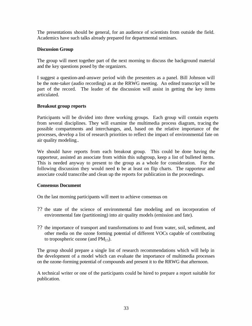
The presentations should be general, for an audience of scientists from outside the field. Academics have such talks already prepared for departmental seminars.
Discussion Group The group will meet together part of the next morning to discuss the background material and the key questions posed by the organizers. I suggest a question-and-answer period with the presenters as a panel. Bill Johnson will be the note-taker (audio recording) as at the RRWG meeting. An edited transcript will be part of the record. The leader of the discussion will assist in getting the key items articulated. Breakout group reports Participants will be divided into three working groups. Each group will contain experts from several disciplines. They will examine the multimedia process diagram, tracing the possible compartments and interchanges, and, based on the relative importance of the processes, develop a list of research priorities to reflect the impact of environmental fate on air quality modeling.. We should have reports from each breakout group. This could be done having the rapporteur, assisted an associate from within this subgroup, keep a list of bulleted items. This is needed anyway to present to the group as a whole for consideration. For the following discussion they would need to be at least on flip charts. The rapporteur and associate could transcribe and clean up the reports for publication in the proceedings. Consensus Document On the last morning participants will meet to achieve consensus on ?? the state of the science of environmental fate modeling and on incorporation of
environmental fate (partitioning) into air quality models (emission and fate). ?? the importance of transport and transformations to and from water, soil, sediment, and
other media on the ozone forming potential of different VOCs capable of contributing to tropospheric ozone (and PM2.5).
The group should prepare a single list of research recommendations which will help in the development of a model which can evaluate the importance of multimedia processes on the ozone-forming potential of compounds and present it to the RRWG that afternoon. A technical writer or one of the participants could be hired to prepare a report suitable for publication.

INTEGRATION OF AIR QUALITY AND
ENVIRONMENTAL MULTIMEDIA MODELING
TASK 3.2
Prepared for:
American Chemistry Council
1300 Wilson Blvd
Arlington, VA 22209
Prepared by:
SENES Consultants Limited
121 Granton Drive, Unit 12Richmond Hill, Ontario
L4B 3N4
May 2005
Printed on Recycled Paper Containing Post-Consumer Fibre

Integration of Air Quality And Environmental Fate Modeling – Task 3.2
33183 – Final – May 2004 i SENES Consultants Limited
TABLE OF CONTENTS
Page No.
SUMMARY ............................................................................................................................S-1
1.0 INTRODUCTION........................................................................................................1-11.1 Background ......................................................................................................1-11.2 Objectives.........................................................................................................1-2
2.0 MODEL SELECTION .................................................................................................2-12.1 Air Dispersion Model, CALMET/CALPUFF modeling system.........................2-1
2.1.1 Overview of the CALPUFF Modeling System.......................................2-22.1.2 CALPUFF Features and Options ...........................................................2-22.1.3 Technical Discussion.............................................................................2-42.1.4 Puff Splitting (Vertical Wind Shear)......................................................2-52.1.5 Integrated Puff Sampling Function Formulation ....................................2-62.1.6 Dry Deposition......................................................................................2-62.1.7 Vertical Structure and Mass Depletion ..................................................2-72.1.8 Wet Removal ........................................................................................2-82.1.9 Input Data Preparation for CALMET/CALPUFF ..................................2-92.1.10 Meteorology........................................................................................2-102.1.11 Terrain Data ........................................................................................2-132.1.12 Land Use.............................................................................................2-14
2.2 Multimedia Model ..........................................................................................2-182.2.1 Fugacity Approach ..............................................................................2-192.2.2 Diffusive Interface Transport...............................................................2-242.2.3 Vegetation...........................................................................................2-252.2.4 Interbox Exchange ..............................................................................2-27
2.3 Atmospheric Reaction Rate.............................................................................2-28
3.0 COUPLING THE MODELS ........................................................................................3-1
4.0 APPLICATION OF THE ORIGINAL AND COUPLED MODELS.............................4-14.1 Chemical Considered ........................................................................................4-14.2 Multimedia Model Input Data...........................................................................4-24.3 Air Emissions ...................................................................................................4-44.4 Ambient Air Monitoring Data...........................................................................4-44.5 Water Quality Data ...........................................................................................4-44.6 Emission Data Sources and Management ..........................................................4-6
5.0 MODELING RESULTS...............................................................................................5-15.1 Ethylbenzene ....................................................................................................5-1
5.1.1 CALPUFF Results ................................................................................5-15.1.2 Multimedia Model Results ....................................................................5-25.1.3 Coupled Model Results .........................................................................5-55.1.4 Comparison of the CALPUFF and Coupled Model Results ...................5-8
5.2 1,3-Butadiene .................................................................................................5-10

Integration of Air Quality And Environmental Fate Modeling – Task 3.2
33183 – Final – May 2004 ii SENES Consultants Limited
5.2.1 CALPUFF Results ..............................................................................5-115.2.2 Multimedia Model Results ..................................................................5-125.2.3 Coupled Model Results .......................................................................5-13
5.3 Atmospheric Availability for Photochemical Degradation...............................5-145.4 Sources of Uncertainty....................................................................................5-15
6.0 SUMMARY AND CONCLUSIONS............................................................................6-1
REFERENCES ....................................................................................................................... R-1
APPENDIX A CALPUFF INPUT FILE

Integration of Air Quality And Environmental Fate Modeling – Task 3.2
33183 – Final – May 2004 iii SENES Consultants Limited
LIST OF TABLES
Page No.
2.1 CALPUFF Layer Heights .............................................................................................2-92.2 Surface and Upper Air Meteorological Stations used as Input into CALMET.............2-102.3 CALMET Land Use Categories Based on the U.S. Geological Survey Land Use
and Land Cover Classification System (52-Category System) ....................................2-152.4 Z Values for Environmental Compartments for Organic Compounds .........................2-212.5 Inter-Compartmental Transport Processes Considered in the Multimedia Model ........2-232.6 Mass Balance Equations.............................................................................................2-23
3.1 Fate and Transport Processes Considered in the Air Compartment ...............................3-1
4.1 Physical/Chemical Properties of Ethyl Benzene and 1,3-Butadiene ..............................4-14.2 Meteorological Data used in the Multimedia Model .....................................................4-24.3 Environmental Compartment Specific Parameters ........................................................4-34.4 Mass Transfer Coefficients and Transport Properties....................................................4-34.5 Summary of Emissions used in Coupled Modeling ......................................................4-8
5.1 Estimated and Ambient Air Concentrations (mg/m3) for Ethylbenzene For
Selected Locations........................................................................................................5-9
5.2 Estimated and Ambient Air Concentrations (mg/m3) for 1,3 Butadiene For
Selected Locations......................................................................................................5-11

Integration of Air Quality And Environmental Fate Modeling – Task 3.2
33183 – Final – May 2004 iv SENES Consultants Limited
LIST OF FIGURES
Page No.
2.1 Puff Splitting................................................................................................................2-62.2 Surface Stations used in the CALMET Modeling .......................................................2-112.3 Upper Air Stations used as Input in the CALMET Modeling ......................................2-122.4 Terrain Data used in CALMET/CALPUFF Modeling.................................................2-132.5 Land Use – Input into CALMET/CALPUFF Modeling ..............................................2-142.6 Wind Flows Vectors from 1995 CALMET Simulation ...............................................2-172.8 The Compartments and Inter-Compartment Transport Terms Considered in
the Multimedia Model ................................................................................................2-22
3.1 The Major Processes Involved in the Coupled Model ...................................................3-23.2A Simplified Flow Chart for the Coupled Multimedia and Air Dispersion Model.............3-33.2B Simplified Flow Chart for the Coupled Multimedia and Air Dispersion Model.............3-4
4.1 Ambient Data and Point Sources of Emission of Ethyl Benzene in Minnesota ..............4-54.2 Ambient 1,3-Butadiene Concentrations for 1999 ..........................................................4-64.3 Ethyl Benzene Air Emission Rates ...............................................................................4-74.4 1,3-Butadiene Air Emission Rates ................................................................................4-8
5.1 Estimated (Lines) and Ambient (Stars) Air Concentrations (mg/m3) for
Methylbenzene – CALPUFF Model .............................................................................5-2
5.2 Estimated (Lines) and Ambient (Stars) Air Concentrations (mg/m3) for
Ethylbenzene – CALPUFF Model ................................................................................5-4
5.3 Estimated Water Concentrations (mg/L) for Ethylbenzene - Multimedia Model ............5-5
5.4 Estimated (Lines) and Ambient (Stars) Air Concentrations (mg/m3) for
Ethylbenzene – Coupled Model....................................................................................5-7
5.5 Estimated Water Concentrations (mg/L) for Ethylbenzene – Coupled Model ................5-8
5.6 CALPUFF/Coupled Model Concentration Ratio Versus Land Use .............................5-10
5.7 Estimated (Lines) and Ambient (Stars) Air Concentrations (mg/m3) for
1,2 Butadiene – CALPUFF Model..............................................................................5-11
5.8 Estimated (Lines) and Ambient (Stars) Air Concentrations (mg/m3) for
1,3-Butadiene – Multimedia Model ............................................................................5-12
5.9 Estimated (Lines) and Ambient (Stars) Air Concentrations (mg/m3) for
1,3-Butadiene– Coupled Model ..................................................................................5-135.10 Maximum Photochemical Degradation of Ethylbenzene and 1,3-Butadiene................5-14

Integration of Air Quality And Environmental Fate Modeling – Task 3.2
33183 – Final – May 2004 S-1 SENES Consultants Limited
SUMMARY
In this study a model that accounts for atmospheric turbulence and describes the transport orpartitioning of VOC to several critical compartments for compounds with relatively shortlifetimes in air was developed. CALPUFF air dispersion model and a multimedia multiboxmodel were used to develop the coupled model. The coupled model was used to assess the effectof atmospheric turbulence and surface partitioning of VOCs on their atmospheric availability forphotochemical degradation.
A calculation domain of 120 by 120 (over Minnesota and Wisconsin) with grid sizes of 5 kmwas selected as large-scale domain. CALPUFF, multimedia model, and coupled model wereused independently to calculate the concentrations, volatilization and photochemical reactionrates of ethylbenzene and 1,3-butadiene. The results from all models were compared for airconcentrations and photochemical reaction rates.
The results indicated that:
1. The CALPUFF, multimedia, and coupled model estimated air concentrations of bothethylbenzene and 1,3-butadiene that were all comparable (within one order of magnitude)to the measured ambient annual average concentrations.
2. The air concentrations estimated with the coupled model were greater than thoseestimated with the CALPUFF model by 10 to 140%.
3. Compared to the CALPUFF model estimated concentrations, the coupled modelestimates were closer to the ambient concentrations. However, due to the uncertainties inthe modeling and emission inventories used in the calculations, it cannot be concludedfirmly that the coupled model results are more accurate.
4. The ratio of the estimated concentrations from coupled and CALPUFF models can betreated as an indication of the degree of revolatilization.
5. The predicted concentration ratios were higher for the boxes with less soil cover andmore vegetation. The ratio varied between 1.1 and 2.9 for various land use ratios.
6. Compared to the ethylbenzene, the ratio of coupled/CALPUFF estimated concentrationsshowed a slight increase of about 10%. This is likely due to the higher vapor pressure andlower water solubility of butadiene compared to ethylbenzene, while the degradationrates of both chemicals at the surface were comparable.

Integration of Air Quality And Environmental Fate Modeling – Task 3.2
33183 – Final – May 2004 S-2 SENES Consultants Limited
7. Inclusion of the atmospheric turbulence in coupled model reduces the availability of bothchemicals studied for atmospheric degradation compared to the original multimediamodel. On average basis, approximately 18% of emitted ethylbenzene and 25% ofemitted 1,3-butadiene were degraded within each grid area. For the coupled model, theaverage degradation rates were 9.5% and 14% for ethylbenzene and 1,3-butadiene,respectively. This difference was mainly attributed to the difference in loss due to theturbulent dispersion and advection processes considered in alternative models.

Integration of Air Quality And Environmental Fate Modeling – Task 3.2
33183 – Final – May 2004 1-1 SENES Consultants Limited
1.0 INTRODUCTION
1.1 BACKGROUND
A Workshop on Combining Environmental Fate and Air Quality Modeling held on June 27 -29,2000 in Research Triangle Park, NC sponsored by the Reactivity Research Working Group(RRWG) of American Chemistry Council (ACC). As a result of a list of research priorities in thearea of multimedia processes that affect the ozone formation potential of volatile organiccompounds (VOCs) capable of contributing to tropospheric ozone was prepare. One researchpriority identified was to create a box model including compartments and transport properties ofcommon environmental fate models and the complex meteorology of air quality models to seewhether the same extent of oxidation is predicted with complex meteorology as with theenvironmental fate model.
The formation of tropospheric ozone is a dynamic multi-step kinetic process that is highlydependent upon the relative concentrations of NOx and volatile organic compounds (VOC). Thetropospheric concentration of a volatile organic compound (VOC) in air is affected by the localsources which release VOCs from area and point sources, by the rate of removal through avariety of competing physical and chemical processes (e.g., photo-oxidation, deposition,horizontal and vertical transport, aerosol formation), by re-volatilization, and by transport intoand out of the local area. Given the concerns over VOCs in the environment, it seems desirableto develop an integrated approach for evaluating the levels of VOCs in the environment throughan integrated evaluation of the various environmental compartments which take account of thevarious atmospheric transport and environmental fate processes.
Air dispersion models have a long tradition of use in atmospheric chemistry to qualitatively andquantitatively evaluate the processes that affect the transport and removal of pollutants from theatmosphere. Air dispersion models have taken a variety of forms and their construction has oftenbeen governed by the specific needs of the investigator and the research problem beingexamined. For example, a model may used detailed or simplified meteorology, aerosolpartitioning, or chemical speciation depending on the type of geographical environment orphotochemical event being evaluated. Although some box models have been developed withdetailed representations of the photochemistry, deposition rates, or aerosol partitioning, to date,none are sufficient to evaluate the impact of surface processes on the atmospheric concentrationsof VOCs.
Many studies indicated that revolatilization is an important process in the fate and transport ofVOCs and semi-volatile organic compounds (SOCs) (Gouin 2003). Beyer and Matthies (2001)presented a combined measure for transport in air and water, considering continuous exchangebetween both compartments due to deposition and revolatilization from the water body. They

Integration of Air Quality And Environmental Fate Modeling – Task 3.2
33183 – Final – May 2004 1-2 SENES Consultants Limited
used the proposed measure to rank chemicals according to their transport potentials in an air-ocean system. Gouin2 showed that the air-surface exchange has a major role in the long-rangetransport of organic contaminants.
Many environmental multimedia fate and transport (multimedia) models have been developed toexamine how a chemical partitions among environmental compartments (e.g. air, water, soil,sediment, and vegetation) (Mackay 1979 and 1991 Diamond et al. 1990 and 1992 and 2001).These multimedia models describe intermedia transport rates for various diffusive and non-diffusive processes and estimate the concentrations of each environmental compartment. Untilnow, these models have not been used to evaluate the effect of complex meteorology and theimpact of VOC emissions on their atmospheric concentrations and availability for formation oftropospheric pollutants. Since existing multimedia models do not have the capability to accountfor turbulent dispersion of such chemicals in atmosphere, multimedia models are not reliabletools to evaluate the air quality parameters.
This report describes the development of a coupled air quality and multimedia model thatincorporates that incorporates atmospheric transport, atmospheric turbulence, and partitioning ofVOCs to several environmental compartments important for VOC compounds with relativelyshort lifetimes in air. The compartments included were an air compartment, an aerosolcompartment, a surface water compartment, a soil compartment and a vegetative compartment.All of the major kinetic processes affecting the emissions to or loss from the air compartment aredescribed. This includes wet and dry deposition, revolatilization from surface, andphotochemical oxidation. The results from the calculations were used to assess the effect ofatmospheric turbulence and surface partitioning of VOCs on their availability for photochemicaldegradation.
1.2 OBJECTIVES
The objective of this study is the development of a model that accounts for atmosphericturbulence and describes the transport or partitioning of VOC to several critical compartmentsfor compounds with relatively short lifetimes in air. These compartments include an aircompartment, an aerosol compartment, a surface water compartment, a soil compartment and avegetative compartment. All of the major kinetic processes affecting the emission to or lossfrom the air compartment are described. This includes wet and dry deposition, revolatilizationfrom surface, and photochemical oxidation. The results from the calculations are used to assessthe effect of atmospheric turbulence and surface partitioning of VOCs on their availability forphotochemical degradation.

Integration of Air Quality And Environmental Fate Modeling – Task 3.2
33183 – Final – May 2004 2-1 SENES Consultants Limited
2.0 MODEL SELECTION
Because the focus of the study is the spatial resolution of the air concentrations, the majorcriteria for selection of the models is their capability of incorporating the needed spatialresolution. Almost all of the multimedia models that have the spatial resolution capability areprepared in a multi-box or multi-grid format. Thus, it is essential that the air dispersion modelchosen for this study is also able to be prepared in a gridded format. After a review of theavailable air dispersion models and examination of their capabilities, the CALMET/CALPUFFmodeling system which is maintained by Earth Tech Inc. was selected as the air dispersionmodel. A multimedia model developed in house by SENES was also selected to be coupled withthe air dispersion model.
2.1 AIR DISPERSION MODEL, CALMET/CALPUFF MODELING SYSTEM
CALMET/CALPUFF (Version 5.5) is a multi-layer, multi-species non-steady-state puffdispersion model which can simulate the effects of time- and space-varying meteorologicalconditions on pollutant transport, transformation, and removal in the atmosphere in a threedimensional gridded domain.
CALMET is a meteorological model that produces hourly, three dimensional gridded wind fieldsfrom available meteorological, terrain and land use data. CALPUFF is a non-steady state puffdispersion model that utilizes the point and area source emission data and CALMET wind fieldsfor calculation of atmospheric concentrations and wet and dry depositions for each grid area.CALPUFF accounts for spatial changes in meteorology, variable surface conditions (terrain andland-use), and plume interaction with simple and complex terrains. In particular:
CALPUFF utilizes complex meteorology information, terrain and land cover data, andemission data in a grided or box format and allows for the calculation of atmosphericconcentrations and both wet and dry depositions for each box. This feature makes itfeasible to couple the air dispersion model with a multibox multimedia model.
CALPUFF has received considerable peer review, as for example, both in a formalizedEPA process (Allwine et al, 1998) and in statements made at the 7th Air QualityModeling Conference. Each of the reviews urged the use of CALPUFF at distancesshorter than 50 kilometers.
CALPUFF is securing its position with US EPA as regulatory model.
On a theoretical basis, CALMET and CALPUFF are applicable to the flat terrain andproduce the comparable results to the ISCST3 model, which is another US EPA’sregulatory model.

Integration of Air Quality And Environmental Fate Modeling – Task 3.2
33183 – Final – May 2004 2-2 SENES Consultants Limited
CALPUFF can treat calm winds and stagnation conditions. It can therefore be expectedthat CALMET/ CALPUFF will not be biased toward underestimates the results.
2.1.1 Overview of the CALPUFF Modeling System
The CALPUFF Modeling System includes three main components: CALMET, CALPUFF, andCALPOST and a set of preprocessing programs designed to interface the model to standard,routinely-available meteorological and geophysical datasets (Scire et al. 2000a and 2000b). Inthe simplest terms, CALMET is a meteorological model that develops hourly wind andtemperature fields on a three-dimensional grided modeling domain. Associated two-dimensionalfields such as mixing height, surface characteristics, and dispersion properties are also producedby CALMET. CALPUFF is a transport and dispersion model that advects “puffs” of materialemitted from modeled sources and simulates dispersion and transformation processes along theway. In doing so, it typically uses the fields generated by CALMET, or as an option, it may usesimpler non-grided meteorological data much like existing plume models. Temporal and spatialvariations in the meteorological fields selected are explicitly incorporated in the resultingdistribution of puffs throughout a simulation period. The primary output files from CALPUFFcontain hourly concentrations and hourly wet and dry deposition fluxes evaluated for each gridor box. CALPOST is used to process these files and to produce summarized simulation results asmonthly or annual average values.
2.1.2 CALPUFF Features and Options
CALPUFF is a multi-layer, multi-species non-steady-state puff dispersion model which cansimulate the effects of time- and space-varying meteorological conditions on pollutant transport,transformation, and removal. CALPUFF can use the three dimensional meteorological fieldsdeveloped by the CALMET model or simple, single station winds. However, the use of single-station winds does not allow CALPUFF to take advantage of its capabilities to treat spatially-variable meteorological fields.
CALPUFF contains algorithms for near-source effects such as building downwash, transitionalplume rise, partial plume penetration, subgrid scale terrain interactions as well as longer rangeeffects such as pollutant removal (wet scavenging and dry deposition), chemical transformation,vertical wind shear, over water transport and coastal interaction effects. It can accommodatearbitrarily-varying point source and grided area source emissions. Most of the algorithms containoptions to treat the physical processes at different levels of detail depending on the modelapplication.

Integration of Air Quality And Environmental Fate Modeling – Task 3.2
33183 – Final – May 2004 2-3 SENES Consultants Limited
CALPUFF contains an optional puff splitting algorithm that allows vertical wind shear effectsacross individual puffs to be simulated. Differential rates of dispersion and transport occur on thepuffs generated from the original puff, which under some conditions can substantially increasethe effective rate of horizontal growth of the plume.
Several options are provided in CALPUFF for the computation of dispersion coefficients,including the use of turbulence measurements, the use of similarity theory, or the use of Pasquill-Gifford (PG) or McElroy-Pooler (MP) dispersion coefficients, or dispersion equations based onthe Complex Terrain Dispersion Model (CDTM). Options are provided to apply an averagingtime correction or surface roughness length adjustments to the PG coefficients.
Some of the major features and options of the CALPUFF model are summarized below.
Source types:
Point sources such as stack (constant or variable emissions); Line sources such as a road (constant or variable emissions); Volume sources such as a large chemical plant (constant or variable emissions); Area sources such as volatilization from a contaminated land (constant or variable
emissions).
Non-steady-state emissions and meteorological conditions:
Grided 3-D fields of meteorological variables (winds, temperature); Spatially-variable fields of mixing height, friction velocity, convective velocity scale,
Monin- Obukhov length, precipitation rate; Vertically and horizontally-varying turbulence and dispersion rates; Time-dependent source and emissions data.
Vertical wind shear:
Puff splitting; Differential advection and dispersion.
Plume rise:
Partial penetration; Buoyant and momentum rise; Stack tip effects; Vertical wind shear; Building downwash effects.

Integration of Air Quality And Environmental Fate Modeling – Task 3.2
33183 – Final – May 2004 2-4 SENES Consultants Limited
Dry Deposition:
Gases and particulate matter; Three options:
o Full treatment of space and time variations of deposition with a resistance model;o User-specified diurnal cycles for each pollutant;o No dry deposition.
Chemical transformation:
Pseudo-first-order chemical mechanism (MESOPUFF II method); User-specified diurnal cycles of transformation rates; No chemical conversion.
Wet deposition:
Scavenging coefficient approach; Removal rate as a function of precipitation intensity and type.
2.1.3 Technical Discussion
Puff models represent a continuous plume as a number of discrete packets of pollutant material.Most puff models (e.g., Ludwig et al., 1977; van Egmond and Kesseboom, 1983; Peterson, 1986)evaluate the contribution of a puff to the concentration at a receptor by a “snapshot” approach(Figure 2.1). Each puff is “frozen” at particular time intervals (sampling steps). Theconcentration due to the “frozen” puff at that time is computed (or sampled). The puff is thenallowed to move, evolving in size, strength, etc., until the next sampling step. The totalconcentration at a receptor is the sum of the contributions of all nearby puffs averaged for allsampling steps within the basic time step. Depending on the model and the application, thesampling step and the time step may both be one hour, indicating only one “snapshot” of the puffis taken each hour.
A traditional drawback of the puff approach has been the need for the release of many puffs toadequately represent a continuous plume close to a source. If the puffs do not overlapsufficiently, the concentrations at receptors located in the gap between puffs at the time of the“snapshot” are underestimated, while those at the puff centers are overestimated.
Two alternatives to the conventional snapshot sampling function are discussed below. Both arebased on the integrated sampling function in the MESOPUFF LI model (Scire et al., 1984a, b),with modifications for near-field applications. The first sampling scheme employs radiallysymmetric Gaussian puffs. The second scheme uses a non-circular puff (a “slug”), elongated inthe direction of the wind during release, to eliminate the need for frequent releases of puffs.
Integration of Air Quality And Environmental Fate Modeling – Task 3.2
33183 – Final – May 2004 2-5 SENES Consultants Limited
CALPUFF allows either of these sampling schemes to be selected, and also allows a hybridsimulation that takes advantage of the strengths of each algorithm (slugs in the near-fieldtransition to puffs in the far-field).
A key modeling consideration in CALPUFF is the specification of the horizontal and verticalGaussian dispersion coefficients for a puff (or each end of a slug) at the start and end of asampling step, and also for each receptor at which the cloud has a computed contribution duringthe step. The coefficients for the puff location at the start of a step are equal to those found at theend of the preceding sampling step, because cloud-size is continuous between sampling steps.Those at the end of the step, or at nearby receptors during the step, are computed according to anambient turbulence growth relationship.
2.1.4 Puff Splitting (Vertical Wind Shear)
Vertical wind shear can sometimes be an important factor affecting plume transport anddispersion. The change of wind speed and wind direction with height causes a differentialadvection of pollutant material emitted at different heights. Even for material emitted at a givenheight, when plumes become large enough, across-plume shear may transport the upper portionof a plume in a different direction than the lower portion. When vertical mixing brings the entireplume to the ground, the effective horizontal dispersion of the plume may be significantlyenhanced as a result of the differential transport. CALPUFF explicitly models wind shear effectson different puffs by allowing each puff to be independently advected by its local average windspeed and direction, and independently mixed vertically to the ground. The average wind for apuff is obtained from profiles of wind speed and direction (available when using CALMETwinds or PROFILE winds) from the top to the bottom of the puff. For example, puffs emittedfrom two sources co-located in the horizontal, but with different release heights will betransported in CALPUFF in different directions and at different speeds if the wind fields indicatesuch a shear exists.
Shear across a single puff is handled in CALPUFF by allowing a well-mixed puff to split intotwo or more pieces when across-puff shear becomes important. Each portion of the puff is thenindependently transported and dispersed. This is illustrated in Figure 2.1. A single puff may besplit multiple times if it remains in the modeling domain long enough. A puff that is stillGaussian in the vertical will not be split. Because across-puff wind shear effects are not likely tobe important in all applications, and because puff splitting increases computational requirements,the puff splitting feature is an option that can be modified or turned off.

Integration of Air Quality And Environmental Fate Modeling – Task 3.2
33183 – Final – May 2004 2-6 SENES Consultants Limited
FIGURE 2.1
PUFF SPLITTING
1000 puffs/hr
Atmospheric layer
Volume Grids
Puff splitting
2.1.5 Integrated Puff Sampling Function Formulation
The detailed formulation of the integrated puff sampling function formulation is described in theCALPUFF user’s manual (Scire et al., 2000a).
2.1.6 Dry Deposition
Many complex processes are involved in the transfer and deposition of pollutants at the surface.The variables include the properties of the depositing material (e.g., particle size, shape, anddensity; gas diffusivity, solubility, and reactivity), the characteristics of the surface (e.g., surfaceroughness, vegetation type, amount, and physiological state), and atmospheric variables (e.g.,stability, turbulence intensity). Hicks (1982) noted the important differences controlling thedeposition of large particles (e.g., gravitational settling, inertial impaction) and those controllinggases (e.g., turbulence, molecular diffusion).
Deposition of small particles is complicated by the fact that they may be influenced by theprocesses affecting both gases and large particles. Due to the number and variability of thefactors influencing dry deposition rates, reported deposition velocities exhibit considerablevariability. For example, SO2 deposition velocity measurements summarized by Sehmel (1980)range over two orders of magnitude. Particle deposition velocities (Slinn et al., 1978) show aneven greater variability. Although it is not practical to include in the deposition model the effectsof all of the variables, it is possible, based on the atmospheric, surface, and pollutant propertiesto parameterize many of the most important effects.
The CALPUFF deposition module provides three options reflecting different levels of detail in

Integration of Air Quality And Environmental Fate Modeling – Task 3.2
33183 – Final – May 2004 2-7 SENES Consultants Limited
the treatment of dry deposition.
A full resistance model is provided in CALPUFF for the computation of spatially and temporallyvarying gas/particle dry deposition rates of gases and particulate matter as a function ofgeophysical parameters, meteorological conditions, and pollutants species.
2.1.7 Vertical Structure and Mass Depletion
The CALPUFF dry deposition model is based on an approach which expresses the depositionvelocity as the inverse of a sum of “resistances” plus, for particles, gravitational settling terms.The resistances represent the opposition to transport of the pollutant through the atmosphere tothe surface. Slinn et al. (1978) describe a multi-layer resistance model for dry deposition. Theatmosphere can be divided into four layers for purposes of computing dry deposition rates. Forgases, an additional (vegetation) layer is included.
(A) Layer Aloft. The top layer is the region above the current mixing height. It containspollutant material either injected directly from tall stacks, or dispersed upward duringprevious turbulent activity. Due to the low rate of turbulent mixing in this layer, itspollutant is essentially cut off from the surface. Therefore, this material is not subject todry deposition until it becomes entrained into the mixed-layer.
(B) Mixed-Layer. The top of the mixed-layer defines the depth of the turbulent boundarylayer. Layer B extends down to a reference height within the atmospheric surface layer.Pollutant mixing is dominated by turbulent processes. During convective conditions,pollutants in this layer quickly become uniformly mixed in the vertical. The resistanceto pollutant transfer during these conditions is very small compared to the resistances inlayers C, D, and F. However, during stable conditions, the mixed-layer resistance maybe substantial (Wesely and Hicks, 1977). The treatment of the mixed-layer resistance isbased on the overall boundary layer diffusivity parameterized in terms ofmicrometeorological scaling variables.
(C) Surface Layer. The surface layer is a shallow layer (10 m or so) next to the ground thatrapidly adjusts to changes in surface conditions. Because vertical fluxes are nearlyconstant, this layer is also called the constant-flux layer. The atmospheric resistance isused to parameterize the rate of pollutant transfer in Layer C.
(D) Deposition Layer. Over very smooth surfaces, a thin non-turbulent layer (the depositionlayer) develops just above the surface. For typically rough surfaces, this layer isconstantly changing and is likely to be intermittently turbulent. For this reason, Hicks(1982) calls this layer the “quasi-laminar” layer. The primary transfer mechanisms

Integration of Air Quality And Environmental Fate Modeling – Task 3.2
33183 – Final – May 2004 2-8 SENES Consultants Limited
across the laminar deposition layer are molecular diffusion for gases, and Browniandiffusion and inertial impaction for particles. However, surface roughness elements(e.g., leaf hairs) can sometimes penetrate the deposition layer, providing an alternateroute for the pollutant transfer (Hicks, 1982). Under conditions of low atmosphericresistance, the deposition layer resistance, rd, can be the dominant resistance controllingthe rate of deposition for particles and some soluble, high molecular weight gases.
(E) Vegetation Layer. Vegetation is a major sink for many soluble or reactive gaseouspollutants. After passing through the stomata, soluble pollutants dissolve in the moistmesophyll cells in the interior of the leaves. Reactive pollutants may also interact withthe exterior (cuticle) of the leaves. Due to the response of the stomata to externalfactors such as moisture stress, temperature, and solar radiation, the resistance in thevegetation layer (i.e., the canopy resistance) can show significant diurnal and seasonalvariability. An alternate pathway that is potentially important in sparsely vegetatedareas or overwater is deposition directly to the ground/water surface. Although notinvolving vegetation, it is convenient to include the ground/water surface resistance as acomponent of canopy resistance because, like the vegetation resistances, it is aresistance in a layer below the laminar deposition layer.
In the CALPUFF model, the fraction of the pollutant mass above and below the current mixedlayer is tracked. At any point in time, only pollutant material below the mixing height can bedeposited at the surface. However, each time step as the mixing height changes, pollutant mass istransferred between Layers A and B. Typically, in the morning, as the boundary layer grows inresponse to solar heating of the land surface, material in the top layer is entrained into the mixed-layer and becomes available for dry deposition at the surface. In the evening, convective activityceases, and material above the shallow nocturnal boundary layer height is isolated until the nextdiurnal cycle. Once puffs have become uniformly mixed through the boundary layer, a surfacedepletion method (Scire et al., 1984b) can be used to account for the mixed-layer (Layer B)resistance.
The details of the full resistance model are described in the CALPUFF user’s manual.
2.1.8 Wet Removal
Many studies have shown that during rain events, wet scavenging of soluble or reactivepollutants can be of the order of tens of percent per hour (Barrie, 1981; Slinn et al., 1978; Levineand Schwartz, 1982; Scire and Venkatram, 1985). Gaseous pollutants are scavenged bydissolution into cloud droplets and precipitation. Particulate pollutants are removed by both in-cloud scavenging (rainout) and below-cloud scavenging (washout). Over source-receptordistances of tens to hundreds of kilometers, wet scavenging can deplete a substantial fraction of

Integration of Air Quality And Environmental Fate Modeling – Task 3.2
33183 – Final – May 2004 2-9 SENES Consultants Limited
the pollutant material from the puff.
An empirical scavenging coefficient approach is used in CALPUFF to compute the depletion andwet deposition fluxes due to precipitation scavenging. The scavenging coefficient depends on thecharacteristics of the pollutant (e.g., solubility and reactivity) as well as the nature of theprecipitation. CALPUFF user’s manual provides the wide range of scavenging coefficient usedin the model calculations.
2.1.9 Input Data Preparation for CALMET/CALPUFF
The CALMET model was used to develop a data set of hourly wind fields for 1995 for use bythe CALPUFF dispersion model. The year 1995 was chosen to match the existing EPA emissiondata base and some available ambient monitoring concentrations in air, water and soil. TheCALMET ran for the large modeling domain of 600 km in east-west direction and 600 km insouth-north direction with the grid spacing (box size) of 5km. This domain mainly coversMinnesota and part of Wisconsin. The results from this calculation were used to capture regionalair flow that was used as an input into the CALPUFF air dispersion calculations. Ten verticallayers were considered in the wind field. The layer heights are shown in Table 2.1.
TABLE 2.1
CALPUFF LAYER HEIGHTS
Vertical Height
of Layer (meters)
Layer Height
at Top (meters)
20 20
20 40
40 80
80 160
160 300
300 600
600 1,000
1,000 1,500
1,500 2,200
2,200 3,000
The mixing heights in “A Mixing Heights Study for North America (1987 –1991)” at TheInternational Falls, Minneapolis and Green Bay were reviewed to insure that the top of the grid iswell above the climatological mixing heights. This pattern of rising layers follows the guidancefrom the user’s manual in terms of gradually increasing layer depth with height.
The CALMET model requires as input, a control file that defines the wind field grid parametersand model option switches, surface and upper air meteorological data, land use data and terrain

Integration of Air Quality And Environmental Fate Modeling – Task 3.2
33183 – Final – May 2004 2-10 SENES Consultants Limited
data. A description of the data used in this analysis is provided below:
2.1.10 Meteorology
The CALMET model used all available meteorology data within a defined modeling domain tocompute girded wind fields. CALMET requires, at a minimum, one surface station and oneupper air (sounding) station. CALMET requires that at least two upper air soundings areavailable, daily, and there is wind and temperature data at the bottom and top layer of themodeling domain. For the study, a complete year (January 1, 1995 – December 31, 1995) isused. Table 2.2 shows the hourly surface meteorological stations as well as the upper air stationsused in analysis. The hourly precipitation data available for eight out of the 10 surface stationsare processed through CALMET to enable CALPUFF to compute wet deposition. Surfacestations without precipitations are: Mason City and Eau Clair.
Surface stations used in the CALMET modeling are presented in Figure 2.2. Upper Air stationsare shown in Figure 2.3.
TABLE 2.2
SURFACE AND UPPER AIR METEOROLOGICAL STATIONS
USED AS INPUT INTO CALMET
1995 Surface Stations
CoordinatesNumber Station name Station Number
Latitude Longitude Easting Northing
1 Duluth 14913 46.833 92.18 334.070 360.187
2 Fargo 14914 46.900 96.80 -4.916 357.890
3 Int'l Falls 14918 48.567 93.38 238.233 541.961
4 La Crosse 14920 43.867 91.25 424.265 46.758
5 Minneapolis 14922 44.883 93.22 267.398 147.205
6 Rochester 14925 43.917 92.00 365.987 48.417
7 St.Cloud 14926 45.550 94.07 200.398 216.280
8 Mason City 14940 43.150 93.33 266.483 -39.147
9 Sioux Falls 14944 43.567 96.73 0.000 0.000
10 Eau Clair 14991 44.867 91.48 399.226 152.707
Upper Air Stations
CoordinatesNumber Station name Station Number
Latitude Longitude Easting Northing
1 Int. Falls 14918 48.567 93.38 238.233 541.961
2 Minneapolis 94983 44.883 93.22 267.398 147.205
3 Green Bay 14898 44.480 88.13 657.865 133.435
4 Aberdeen 14929 45.450 98.42 -127.048 203.546
5 Omaha/Valley 94980 41.320 96.37 29.352 -241.563

Integration of Air Quality And Environmental Fate Modeling – Task 3.2
33183 – Final – May 2004 2-11 SENES Consultants Limited
FIGURE 2.2
SURFACE STATIONS USED IN THE CALMET MODELING
LAKE SUPERIOR
Meteorological Surface Stations Usedas Input in the CALMET
Modelling Domain 600 x 600 km
0 100 200 300 400 500
0
100
200
300
400
500
DulluthFargo
Int'l Falls
La Crosse
Minneapolis
Rochester
St.Cloud
Mason City
Sioux Falls
Eau Clair

Integration of Air Quality And Environmental Fate Modeling – Task 3.2
33183 – Final – May 2004 2-12 SENES Consultants Limited
FIGURE 2.3
UPPER AIR STATIONS USED AS INPUT IN THE CALMET MODELING
LAKE SUPERIOR
Meteorological Upper Air Stations Usedas Input in the CALMET
Modelling Domain 600 x 600 km
-100 0 100 200 300 400 500 600
-200
-100
0
100
200
300
400
500
Int. Falls
MinneapolisGreen Bay
Aberdeen
Omaha/Valley

Integration of Air Quality And Environmental Fate Modeling – Task 3.2
33183 – Final – May 2004 2-13 SENES Consultants Limited
2.1.11 Terrain Data
Girded terrain data for the large modeling domain are available in 30 arc-seconds (~900mspacing through the United States Geological Survey (USGS) Internet site.) . This data weredownloaded from the USGS and processed into CALMET formats using the terrain-processingprogram TERREL that is provided with the CALMET/CALPUFF modeling system. A map ofthe terrain data is shown in Figure 2.4.
FIGURE 2.4
TERRAIN DATA USED IN CALMET/CALPUFF MODELING
0 50 100 150 200 250 300 350 400 450 500 550
Easting (km)
0
50
100
150
200
250
300
350
400
450
500
550
Nort
hin
g (
km)
LAKE SUPERIOR
Terrain on 5 x 5 km Grid - Lambert Conformal ProjectionCoordinate Origine at (Lat=43.567deg and Lon.=96.736; Sioux Falls)
Modelling Domain 600 x 600 km

Integration of Air Quality And Environmental Fate Modeling – Task 3.2
33183 – Final – May 2004 2-14 SENES Consultants Limited
2.1.12 Land Use
Digital Composite Theme Grid (CTG) Land Use and Land Cover (LULC) data, at the globalscale (900m resolution), available from the USGS, were used to determine land use data forCALMET. These data were processed with the CTGPROC land use processor program. Theseland use categories are listed in Table 2.3. Figure 2.5 shows the land use in the modeling domain.
FIGURE 2.5
LAND USE CATEGORIES – INPUT INTO CALMET/CALPUFF MODELING BASED
ON GLOBAL LAND USE – GRID 5 KM LAMBERT CONFORMAL PROJECTION
10-Urban 60-Wet Land20-Agricultural 70-Barren Land30-Range Land 80-Tundra40-Forest Land 90-Perennial Snow or Ice50-Water

Integration of Air Quality And Environmental Fate Modeling – Task 3.2
33183 – Final – May 2004 2-15 SENES Consultants Limited
TABLE 2.3
CALMET LAND USE CATEGORIES BASED ON THE U.S. GEOLOGICAL SURVEY
LAND USE AND LAND COVER CLASSIFICATION SYSTEM (52-CATEGORY
SYSTEM)
Level I Level II
10 Urban or Built-upLand
11121314151617
ResidentialCommercial and ServicesIndustrialTransportationCommunications and UtilitiesIndustrial and CommercialComplexesMixed Urban or Built-up LandOther Urban or Built-up Land
20 Agricultural Land -Unirrigated
2122
2324
Cropland and PastureOrchards, Groves, Vineyards,Nurseries, andOrnamental Horticultural AreasConfined Feeding OperationsOther Agricultural Land
!20 Agricultural Land -Irrigated
2122
2324
Cropland and PastureOrchards, Groves, Vineyards,Nurseries, andOrnamental Horticultural AreasConfined Feeding OperationsOther Agricultural Land
30 Rangeland 313233
Herbaceous RangelandShrub and Brush RangelandMixed Rangeland
40 Forest Land 414243
Deciduous Forest LandEvergreen Forest LandMixed Forest Land
50 Water 5152535455
Streams and CanalsLakesReservoirsBays and EstuariesOceans and Seas

Integration of Air Quality And Environmental Fate Modeling – Task 3.2
33183 – Final – May 2004 2-16 SENES Consultants Limited
TABLE 2.3 (Cont’d)
CALMET LAND USE CATEGORIES BASED ON THE U.S. GEOLOGICAL SURVEY
LAND USE AND LAND COVER CLASSIFICATION SYSTEM (52-CATEGORY
SYSTEM)
Level I Level II
60 Wetland 6162
Forested WetlandNonforested Wetland
70 Barren Land 71727374757677
Dry Salt FlatsBeachesSandy Areas Other than BeachesBare Exposed RockStrip Mines, Quarries, andGravel PitsTransitional AreasMixed Barren Land
80 Tundra 8182838485
Shrub and Brush TundraHerbaceous TundraBare GroundWet TundraMixed Tundra
90 Perennial Snow orIce
9192
Perennial SnowfieldsGlaciers
Figures 2.6 shows one example of wind flows vectors from 1995 CALMET simulation for onehour (July 15, 00:00 and July 15, 13:00).

Integration of Air Quality And Environmental Fate Modeling – Task 3.2
33183 – Final – May 2004 2-17 SENES Consultants Limited
FIGURE 2.6
WIND FLOWS VECTORS FROM 1995 CALMET SIMULATION
50 100 150 200 250 300 350 400 450 500 550
50
100
150
200
250
300
350
400
450
500
550
CALMET SIMULATION -Jul 15, Hour 01:00 AM, 1995
Reference Vectors
0.01 5.7 m/s

Integration of Air Quality And Environmental Fate Modeling – Task 3.2
33183 – Final – May 2004 2-18 SENES Consultants Limited
2.2 MULTIMEDIA MODEL
Once a chemical is introduced to the environment it distributes among the environmentalcompartments. The extent that the chemicals partition among the environmental compartmentsdepends on the environmental conditions (e.g. temperature, precipitation rate) and thephysical/chemical properties of the chemical, (e.g. Kow and Koa for organic and Kd for metals).While some chemicals tend to build up in one compartment, others end up partitioning amongother compartments. The latter are referred to as multimedia chemicals. Among thesecontaminants volatile organic compounds (VOCs), semi volatile organic compounds (SOCs),persistent organic pollutants (POPs), and some metals have been extensively studied.Understanding the fate of these groups of chemicals requires modeling their behavior in all of theenvironmental compartments. This is what is referred to as multimedia environmental modeling.
Formulation and results of multimedia models are quite sensitive to the size and resolution of thesite studied. The scale for such models could be a small site (local) or regional, or larger (lake orcontinental models). Multimedia models that have the capability of spatial resolution areprepared in a grided or multi-box format.
The model that was considered for this study was a modified version of a multi-box multimediaregional model that can handle the domains as large as several hundred kilometers and has theresolution of few kilometers.
The modified version of the multimedia model used in this study accounts for five bulkcompartments: air, surface water, surface soil , sediment underlying the surface water , andvegetation . Each bulk compartment may consist of sub-compartments of specified volume.Chemicals are assumed to be in equilibrium between these sub-compartments within each bulkcompartment (e.g., between water and suspended particles in surface water compartment).Equilibrium is not assumed among compartments. The multimedia model assume that a uniformsteady-state concentration is achieved in each compartment in each box.
The model establishes a set of mass balance equations for each compartment and solves themsimultaneously to obtain the concentration of the contaminant in each compartment, as well asthe fluxes of contaminant across the inter-compartmental interface. The fugacity approach firstintroduced by Mackay (1979, 1991) is efficient tool to solve the mass balance equations and wasused in developing the model.
The model was prepared in a multibox framework in which the domain divided into boxes inorder to allow spatial resolution. The model, therefore, utilizes the box specific landscape data toprovide more precise concentration. The model uses the Digital Composite Theme Grid (CTG)Land Use and Land Cover (LULC) data, at the global scale (900m resolution) to calculate the

Integration of Air Quality And Environmental Fate Modeling – Task 3.2
33183 – Final – May 2004 2-19 SENES Consultants Limited
land use fractions for each box. The calculated area of each category is used to calculate thedistribution of the chemicals at the surface compartments in each box.
The modified version of the model uses a pseudo steady-state approach to interact with the airdispersion model during the execution of the coupled model. A steady-state formulation issuitable in circumstances when model parameters are relatively constant. This is reasonable forsoil and sediment that respond slowly to changes such as variations in loadings. However, airand water compartments respond quickly to the environmental changes (for VOCs) and areunlikely to achieve steady state. When time frame of calculation is short (e.g. less than a day), apseudo-state-state approach can be used to handle the unsteady-state conditions using musheasier steady-state formulation. Average, constant conditions are used during each time intervalof the calculations. This approach also helps to overcome the difficulties arising from the largedifference in time constants among the “slowly” and “quickly” responding compartments.
2.2.1 Fugacity Approach
Fugacity has units of pressure and can be regarded physically as the partial pressure or escapingpotential exerted by a chemical in one physical phase or compartment on another (Mackay, 1979,1991; Mackay and Paterson, 1981, 1982). When two or more compartments are in equilibriumthe fugacity of a chemical is the same in all phases. This characteristic of fugacity-basedmodeling often simplifies the mathematics involved in calculating partitioning. In an equilibriumsystem, calculating several concentrations in various environmental compartments is replaced bycalculating a single fugacity value. Fugacity models can also be used to represent a dynamicsystem in which the fugacities in two adjacent compartments are changing in time due to animbalance of gains and losses or a dynamic system that has achieved steady state by balancinggains and losses even though fugacities are not equal.
At low concentrations, like those typical of environmental concentrations, fugacity, ƒ (Pa), islinearly related to concentration C (mol/m3) through the fugacity capacity, Z (mol/m3-Pa),
C = ƒZ (1)
Based on the fugacity approach, the transport processes are expresses mathematically as a newterm that is called D value. This value is defined as:
D = GZ (2)
Where G (mol/h or kg/h) is the mass or molar flux. Hence inter-compartmental chemicalexchange can be expresses as:
m = GC = fZD/Z = fD (3)

Integration of Air Quality And Environmental Fate Modeling – Task 3.2
33183 – Final – May 2004 2-20 SENES Consultants Limited
where m is molar flux or mass transfer rate of the chemical.
Calculating Z Values
Z value depends on the physical and chemical properties of the chemical and on variouscharacteristics of phase, such as temperature and density. The property that fugacities are equalat equilibrium allows for simple determination of Z values from partition coefficients, K12. Forexample for two phases in equilibrium (phase 1 and 2):
C1 /C2 = ƒZ1 /ƒZ2 = Z1 /Z2 = K12 (4)
The traditional fugacity approach was developed for non-ionic organic chemicals. For this groupof chemicals with measurable vapor pressure, the pure air compartment is the starting point forcalculating Z values, for low concentrations, the fugacity of a chemical in air is the same as itspartial pressure. Thus:
Za = 1/RT (5)
Where R is the universal gas constant and T is absolute air temperature. Consequently, the Zvalues for water, soil, and sediments can be calculated using Henry’s Law Constant and partitioncoefficients, respectively. During last decade researchers have developed relationships for Zvalues for other environmental compartments, such as aerosol (Harner and Bidelman 1998) andvegetation, based on experimental data. Bulk Z values are calculated using sub-compartmental orpure Z values and volume fractions:
iibulkvZZ Â= (6)
where v is the volume fraction of each sub-compartment. Table 2.4 indicates the equations tocalculate the organic chemicals Z value for various environmental compartments.

Integration of Air Quality And Environmental Fate Modeling – Task 3.2
33183 – Final – May 2004 2-21 SENES Consultants Limited
TABLE 2.4
Z VALUES FOR ENVIRONMENTAL COMPARTMENTS FOR ORGANIC
COMPOUNDS
Compartment Phase Equation
Air
Gas PhaseParticulate(1)
Bulk
ZA = 1/RT
ZQ = 10^(log KOA + log fom – 11.91) ¥ ZA ¥ r ¥ 109
ZBA = ZA + (ZQ ¥ vQ)
Water
DissolvedSuspended Part.
Bulk
ZW = 1/H*
ZP = ZW ¥ r ¥ KOC ¥ foc
ZBW = ZW + (ZP * vP)
SoilSolidsBulk
ZS = ZW ¥ r ¥ 0.41KOW ¥ foc
ZBS = (vA ¥ ZA) + (vW ¥ ZW) + (vS ¥ ZS)
SedimentSolidsBulk
ZD = ZW ¥ r ¥ 0.41KOW ¥ foc
ZBD = (vW ¥ ZW) + (vD ¥ ZD)
VegetationLeaf Cuticle
BulkZV = ZW ¥ KOW¥ foc
ZBV = (vA ¥ ZA) + (vW ¥ ZW) + (vV ¥ ZV)
(1) Harner and Bidleman (1998)KOW Octanol-water partition coefficientKOC Organic carbon-water partition coefficientKOA Octanol-air partition coefficientfom Organic matter fractionfoc Organic carbon contentH Henry’s law constant
r Density of compartment
Figure 2.7 shows the processes considered in the fate and transport model and Table 2.5describes these processes.

Integration of Air Quality And Environmental Fate Modeling – Task 3.2
33183 – Final – May 2004 2-22 SENES Consultants Limited
FIGURE 2.7
THE COMPARTMENTS AND INTER-COMPARTMENT TRANSPORT TERMS
CONSIDERED IN THE MULTIMEDIA MODEL
R: Degradation reactions
B: Sediment burialL: Soil leaching to the groundwater
Vegetation Air
Water Soil
Sediments
R
R RL
R
RB

Integration of Air Quality And Environmental Fate Modeling – Task 3.2
33183 – Final – May 2004 2-23 SENES Consultants Limited
TABLE 2.5
INTER-COMPARTMENTAL TRANSPORT PROCESSES CONSIDERED IN THE
MULTIMEDIA MODEL
Inter-compartment transport Individual processes
Air-VegetationWet depositionDry depositionBi-directional diffusion
Air-Surface soilWet depositionDry depositionBi-directional diffusion
Air-Surface waterWet depositionDry depositionBi-directional diffusion
Vegetation-Surface water Canopy drip/leaf wash off
Vegetation-Surface soilCanopy drip/leaf wash offWax erosionLitter fall
Surface soil-Surface water Soil run off (dissolved and suspended phases)
Lake-SedimentsBi-directional diffusionSediment resuspensionSediment deposition
Table 2.6 shows the mass balance equations in the multimedia model.
TABLE 2.6
MASS BALANCE EQUATIONS
No. Compartment Mass Balance Equations
1 Air A1+E1+F5¥D5-1+F3¥D3-1+F2¥D2-1 = F1¥ ( R1+S1+D1-5+D1-3+D1-2)
2 Lake water F1¥D1-2+F3¥D3-2+F4¥D4-2 = F2¥ (R2+D2-1+D2-4)
3 Soil F1¥D1-3+F5¥D5-3 = F3¥ (R3+D3-1+D3-2)
4 sediments F2¥D2-4 = F4¥ (R4+B4+D4-2)
5 Vegetation F1¥D1-5 = F5¥ (R5+D5-1+D5-3)
A: AdvectionD: D valueZ: Bulk Z value

Integration of Air Quality And Environmental Fate Modeling – Task 3.2
33183 – Final – May 2004 2-24 SENES Consultants Limited
F: FugacityR: ReactionB: Burial
L: LeachingS: Vertical Loss
2.2.2 Diffusive Interface Transport
Bi-directional gas phase transfer is modeled using the conventional two-film theory. When twocompartments, such as surface water and air, are in contact, the mass transfer from air to water(or from water to air) depends on mass transfer through both the air-side and water-sideboundary layers. The overall resistance to mass transfer through the two boundary layers is thesum of the two resistances through the air and water boundary layers. The mass-transferresistance is proportional to the inverse of the mass transfer coefficient.
U = [1/(Ua) + 1/(Uw)]-1 (7)
The mass transfer coefficient at each side can be written as a function of effective diffusioncoefficient and boundary layer thickness in each side.
Ua = Da /da (8)
Uw = Dw /dw (9)
where Da is the diffusivity in the air compartment, m2 /s; da is the boundary-layer thickness in the
air above water, m; where Dw is the effective diffusivity in the water compartment, m2 /s; and dw
is the boundary-layer thickness in the water below the air, m, the relationships derived in thissection for mass transfer at the air-water interface can be generalized to mass transfer at air-soil,soil-soil, and water-sediment interfaces.
There is a discontinuity in concentration at this boundary because the concentration at theinterface reflects the equilibrium partitioning of contaminant concentration in the differentphases. In contrast, the fugacity is continuous across this interface. Thus above equations can bemodified to be used in fugacity approach:
U Z= [1/(ZaUa) + 1/(ZwUw)]-1 (10)
Diffusive mass transfer at the air and surface-water interface
The exchange of chemicals between air and water bodies depends on both the physicochemicalproperties of the contaminant and the physical properties of the air and water compartmentsinvolved. Important physicochemical properties include solubility, molecular weight, vapor

Integration of Air Quality And Environmental Fate Modeling – Task 3.2
33183 – Final – May 2004 2-25 SENES Consultants Limited
pressure, and diffusion coefficients in air and water. The important landscape properties includetemperatures of air and water, wind speed, water-flow velocity, water depth, and waterturbulence.
Lyman et al. (1982) have reviewed several methods for estimating water-side and gas-side masstransfer coefficients for atmosphere-surface water exchange of organic chemicals. Theestimation of the air-side and water-side boundary mass-transfer coefficient can be based onmethods developed by Southworth (1979) from laboratory data. In this method the mass transfercoefficient is a function of current and wind velocity as well as chemical molecular weight.
Diffusive mass transfer in air at the air and ground-surface soil interface
Diffusive mass transfer at the soil-air interface accounts for both net volatilization ofcontaminants from soil and deposition of gas-phase contaminants to the ground-surface-soillayer. Once again, net mass transfer depends on mass transfer through both the air-side andground-soil-side boundary layers. The boundary layer thickness in the air above the ground-soillayer thickness is assumed to be on the order of 0.005 m. On smooth surfaces the boundary layerthickness varies from about 1 cm in still air to 1 mm when the air moves over the surface at1 m/s (Hanna et al., 1982).
Diffusive mass transfer at the surface-water and sediment interface
Formica et al. (1988) have described a method for calculating for the sediment layer effectivediffusivity based on corrections for the solids content of sediment. This approach is similar tothat used by Jury et al. (1983) for soil with the volume fraction of the gas phase set to zero.Boundary layer thickness can be calculated using Jury et al. method.
2.2.3 Vegetation
Numerous studies have investigated contaminant transport within the air-vegetation-soil system.We should incorporate work that focuses on processes such as vegetative canopy interception(Gash et al., 1995, Carlyle-Moses et al., 1999, Mahendrappa, 1990) and contaminant partitioningbetween air and leaves, air and soil, and between soil and root systems (Simonich and Hites1995, Trapp and Matthies 1997).
We first consider canopy interception for wet and dry conditions which is parameterized as thefraction of chemical, on an aerial basis, that is deposited on leaves. The dry depositioninterception fraction, IfD, is taken from Whicker and Kirchner (1987),
IfD = 1 - exp(-2.8 B) (11)

Integration of Air Quality And Environmental Fate Modeling – Task 3.2
33183 – Final – May 2004 2-26 SENES Consultants Limited
where B is the above ground biomass of vegetation (kg dry mass/m2). The wet depositioninterception fraction, IfW, depends on the leaf area index (LAI), and the interception coefficient,
a . IfW can vary substantially with meteorological conditions and canopy density (Müller and
Pröhl, 1993),
IfW = LAI ¥ a ¥ (1 - exp ( -ln2/3 1/a)) (12)
IfD and IfW are then multiplied by the terms for dry and wet particle deposition to a surface,respectively. The wet deposition interception loss fraction (IlW) defined as the fraction of totalincident precipitation which evaporates off the leaf surface and consequently, does not make it tothe soil below. The fraction of contaminants not intercepted at all by the vegetative canopy, freethroughfall, is assumed be transported directly from the air to soil (Gash et al. 1995).
Under wet conditions contaminants transport between vegetation and soil occurs via canopy dripwhich is the wet removal of particulates from vegetation due to the impact of rainfall. The masstransfer coefficient for this process, UCD (m/h) is described by,
UCD = RR (IfW-IlW) l (13)
where RR is the rain rate (m/h), IfW and IlW are the wet deposition interception and loss fractions
respectively, and l is the canopy drip parameter which is related to the efficiency of the removal
of particulates from the leaf surface. We have assumed that a given fraction of the leaf surface iscovered by particles and that, for any given rain event, only a small fraction of these particles areremoved. We believe this to be due to some leaf bound particles residing in pits and cracks in theepicuticular wax structures (Turunen and Huttunen 1990), and hence, are minimally removed byprecipitation.
Under dry conditions two processes convey chemicals from vegetation to soil. First, litterfalloccurs in which dead or decaying leaf matter falls from trees to the ground below. This process isassumed to be controlled by a first order rate constant, (RLF) which is taken to be 1/LG where LG
is the length of the growing season (Bennett et al. 1998). In urban centers litterfall is typicallycollected and disposed of outside the city boundary making it a permanent removal process forchemicals in the system. The second process which transports contaminants from vegetation tosoil is that of wax erosion whereby a portion of the leaf surface itself is physically removed.Several researchers (Van Gardigen et al. 1991, Rogge et al. 1993, Horstmann and McLachlan,1996) have concluded that wind and wind-borne particulate abrasion and/or the rubbing motionsof leaves against each other can dislodge contaminant enriched, crystalline-like leaf surfacewaxes.

Integration of Air Quality And Environmental Fate Modeling – Task 3.2
33183 – Final – May 2004 2-27 SENES Consultants Limited
Finally, the model considers bi-directional diffusive exchange of gas-phase chemicals betweenair and cuticle. This was modeled analogously to air-film exchange by using the Whitman two-film theory. The air-side mass transfer coefficient for vegetation is calculated similarly to that for
the film, substituting a value of 4 for b for vegetative surfaces as outlined in Nobel (1991).
2.2.4 Interbox Exchange
If the multimedia / multibox model is a stand-alone model which is not coupled with airdispersion model, it requires a simple air dispersion module to allow spatial resolution, or morespecifically, to estimate chemical transport across box boundaries as well as losses to thestratosphere. Most of the models use prevalent wind direction and average wind velocity tocalculate the advection term. The interbox exchange of the chemicals occurs through advectiveprocesses in the air compartment.
In the stand alone multimedia / multibox model that was used in this study, the air compartmentis divided into two vertical layers in each segment based on the available information of theminimum and maximum mixing height in the morning and afternoon, respectively. The heightof the lower layer equals the minimum mixing height and the upper layer height equals thedifference between the maximum and minimum mixing height minus the height of the lowerlayer. In the afternoon, the mixing height increases resulting the expansion of the contaminatedatmosphere. Overnight, the mixing height decreases resulting in the loss of some of thechemicals. This cyclic “ventilation” mechanism results in net vertical loss of chemical from theair compartment. Assuming vertically mixed atmospheric layer the net loss of the chemical canbe calculated as follows.
Contaminants are considered to move between boxes via movement of air masses along the winddirection and turbulent dispersion across the wind direction. A simplified K (Gradient transport)model (Hanna 1968) was used to calculate the crosswind dispersion rate of contaminants. In thismodel turbulent fluxes of Contaminant C are assumed to be proportional to the mean gradient ofC. The continuity equation for two-dimensional (vertical direction is assumed well mixed), time-independent, and continuous ground-level source can be written as follows:
2
2
Y
CK
X
Cu
Y= (14)
For a simple case of constant u and KY the solution for this equation is Gaussian as follows:

Integration of Air Quality And Environmental Fate Modeling – Task 3.2
33183 – Final – May 2004 2-28 SENES Consultants Limited
˜̃¯
ˆÁÁË
ʘ̃¯
ˆÁÁË
Ê=
XK
uY
XK
u
u
QC
YY 4exp
423.1
22/1
(15)
This form of solution has Gaussian form with standard deviation of the distribution (sY) given by
the equation2/1
2˜¯ˆ
ÁËÊ=
u
XKY
Ys or
X
uK
Y
Y
2
2s
= (16)
Briggs (1973) developed the following empirical formula to calculate sY in urban conditions:
2/1)0004.01( -+= XmX
Ys (17)
For distances greater than 5 km (the size of the boxes in this study) I can be neglected and theequation will be reduced to:
2/150mX
Y=s (18)
Substituting this equation in Equation 16 will yield:
umKY
21250= (19)
Thus the crosswind dispersion term can be formulated using the following equation
XAKdispersionCrosswind Y
D=
21 (20)
When the model is coupled with CALPUFF the above simplified air dispersion module isremoved from the model and the spatial resolution in air concentrations is determined byCALPUFF air dispersion model.
2.3 ATMOSPHERIC REACTION RATE
Photochemical oxidation of VOCs is modeled using Atkinson method (Atkinson 1994). In thismethod the degradation of chemicals follows a first order chemical reaction and is a function ofthe concentration of hydroxyl radicals in the atmosphere. The temperature was assumed to beconstant and uniform in the air compartment and the reaction rate depends upon the chemicaland hydroxyl radical concentrations.

Integration of Air Quality And Environmental Fate Modeling – Task 3.2
33183 – Final – May 2004 2-29 SENES Consultants Limited
Reaction rate = kOH [OH] [chemical] (21)
The concentration of hydroxyl radicals depends greatly on the amount of sunlight available. Atypical figure is approximately 2_106 molecules/cm3 in summer months and1_106 molecules/cm3 in winter months (Singh et al., 1986). At night the concentration ofhydroxyl radicals is negligible.

Integration of Air Quality And Environmental Fate Modeling – Task 3.2
33183 – Final – May 2004 3-1 SENES Consultants Limited
3.0 COUPLING THE MODELS
The original multimedia model is initialized with the “emission” of chemicals to air, surfacewater, and soil as the input. In order to couple the model with CALPUFF the chemical input tothe surface compartments (soil and surface water) was replaced to “wet and dry deposition”calculated by CALPUFF. The multimedia model in the coupled mode uses the deposition valuesand calculated the distribution of the chemical among the surface environmental compartmentsas well as the intermedia transport rates including surface volatilization. No other emissions areassumed to be handled by the fate and transport module. The volatilization from the surfacescalculated by the multimedia model in the coupled mode is considered as new area source ineach box. Calculated volatilization as well as other area and point sources are then used as inputto the CALPUFF in coupled mode. The CALPUFF then calculates the air concentrations and thewet and dry deposition rates. This process will be repeated in an interactive manner between twomodels in the coupled mode for the entire calculation period. The communication of both modelsoccurred at every 24-hr calculation time. Table 3.1 compares the fate and transport processesconsidered in the air compartment for three models discussed above.
TABLE 3.1
FATE AND TRANSPORT PROCESSES CONSIDERED IN THE AIR COMPARTMENT
Multimedia Model CALLPUF Model Coupled Model
Wet Deposition Wet Deposition Wet DepositionDry Deposition Dry Deposition Dry DepositionAdvection (in theprevalent wind direction)
Multi-directional turbulentdispersion (Advection)affected by wind field
Multi-directional turbulentdispersion (Advection)affected by wind field
Photochemical reaction Photochemical reaction Photochemical reactionRevolatilization - Revolatilization
A pre-processor (crearea.exe) prepares an updated area emission file based on the surfacevolatilization values to be used by CALPUFF in the next 24-hr calculation period. In order tocouple both models, the following specific modifications were done to both models:
Dry and wet depositions were calculated through CALPUFF model. However, drydeposition calculations in CALPUFF have been modified for each box to account for bi-directional diffusion at the air-surface interface.
The simplified air dispersion module in the multimedia model was removed. A new module has been developed to account for cumulative deposition on each
environmental compartment.

Integration of Air Quality And Environmental Fate Modeling – Task 3.2
33183 – Final – May 2004 3-2 SENES Consultants Limited
A new CALPUFF emission file has been created to accept the volatilization of chemicalsfrom vegetation, soil surface, and surface waters, as new emission sources whenconsidering complex meteorology.
The land use categories used in CALPUFF with those used in the multimedia model weremade consistent.
The grid generation (size and quantity) module in the multimedia model was modified inconsistency with CALPUFF grid system.
The time step calculations in the dynamic mode of the multimedia model were modifiedin accordance with CALPUFF time steps.
Dry and wet deposition modules in the multimedia model were replaced with thecalculated values in CALPUFF part of the coupled model.
Figure 3.1 indicates the major processes involved in the coupled model and Figure 3.2 indicatesa simplified flow chart of the coupled model calculations.
FIGURE 3.1
THE MAJOR PROCESSES INVOLVED IN THE COUPLED MODEL
Air
SoilVegetation Sediments
Surface water
Volatilization VolatilizationVolatilization
Wet/Dry
Deposition
Wet/Dry
Deposition
Wet/Dry
Deposition
Run off
Particle
Deposition
Sediment
Resuspension
Leaf Fall
Wash off
CALPUFF Model
Multimedia Fate Model
Atmospheric
Dispersion
Next Box

Integration of Air Quality And Environmental Fate Modeling – Task 3.2
33183 – Final – May 2004 3-3 SENES Consultants Limited
FIGURE 3.2A
SIMPLIFIED FLOW CHART FOR THE COUPLED MULTIMEDIA AND AIR
DISPERSION MODEL
Yes No
Start
Set up the box information
Set up the land use categories for each box
Complex meteorology ?
Set up phys/chem and transport properties
Set up emission data (point source and area source)
Set up a simple air dispersion scheme based
on average wind speed and direction
A
Report the results
Calculate surface to air transport rate
Program end
B
Time 0
Run the puff model to calculate the
Air concentrations and deposition rates
Adjust the emission data Based on
the calculated volatilization rates
Last time increment ?
Add time increment
YesNoCalculate the time average
concentrations and report the results

Integration of Air Quality And Environmental Fate Modeling – Task 3.2
33183 – Final – May 2004 3-4 SENES Consultants Limited
FIGURE 3.2B (Cont’d)
SIMPLIFIED FLOW CHART FOR THE COUPLED MULTIMEDIA AND AIR
DISPERSION MODEL
Set up the hourly meteorological data
and generate the windfield
Set up the time domain and time
increment and boundary conditions
Set up the terrain and precipitation data
B
Set up mass balance equations for air /
surface water / soil / vegetation / sediments
for each box
Solve the set of equations for concentrations
in environmental compartments by iterative method
Calculate the deposition rates and
Inter-compartmental transport rates
A

Integration of Air Quality And Environmental Fate Modeling – Task 3.2
33183 – Final – May 2004 4-1 SENES Consultants Limited
4.0 APPLICATION OF THE ORIGINAL AND COUPLED MODELS
As a case study, a calculation domain of 120 by 120 grid points over Minnesota and Wisconsinwith a 5-km grid spacing was selected. Meteorological and land use data were collected for thisdomain. Area and point sources of emissions for ethylbenzene and 1,3-butadiene for the domainwere identified. CALPUFF, the multimedia model, and the coupled model were each usedindependently to calculate the air concentrations, surface volatilization and photochemicalreaction rates.CALPUFF input file used in this study is provided in APPENDIX A.
In order to simplify the calculations, the emissions outside the calculation domain were notconsidered. Due to lack of information, the emissions to the surface water within the calculationdomain as well as background concentrations were not considered.
CALPUFF model produces multibox air concentrations. Multimedia model produced multiboxair, soil, and water concentrations as well as photochemical reaction rates. Coupled modelproduced multibox air, soil, and water concentrations as well as photochemical reaction rates.The results from all models were compared for air concentrations and photochemical reactionrates.
4.1 CHEMICAL CONSIDERED
Ethylbenzene and 1,3-butadiene have been selected for this study. These two chemicalsrepresent two groups of linear and aromatic VOCs. Table 4.1 shows the physical/chemical dataused in the model for both models.
TABLE 4.1
PHYSICAL/CHEMICAL PROPERTIES OF ETHYLBENZENE AND 1,3-BUTADIENE
Parameter Ethylbenzene Butadiene
Molecular Weight 106.2 54.1
Melting Point, C -95 -109
Solubility, g/m3 174.328 1000
Vapour_Pressure at 25 C, pa 1276.695 2450000
Log_Kow 3.124 1.99Diffusion Coefficient in Water, cm2/sec 8.87E-06 1.11E-05Diffusion Coefficient in Air, cm2/sec 7.50E-02 8.75E-02
Ethylbenzene is oxidized in the atmosphere relatively quickly via free-radical chain reactions.The most important radical involved in the oxidation of ethylbenzene is the hydroxyl (OH)radical, but ethylbenzene also reacts with other species, such as alkoxy radicals, peroxy radicals,ozone and nitrogen oxides. Half-life of ethylbenzene in the atmosphere has been estimated from

Integration of Air Quality And Environmental Fate Modeling – Task 3.2
33183 – Final – May 2004 4-2 SENES Consultants Limited
smog chamber experiments and from knowledge of the reaction rate constant for reaction withhydroxyl radicals.
Singh et al. (1981, 1983) reported a half-life of one day with 12 hours sunlight hours. Anotherstudy (Callahan, 1979) reported an atmospheric half-life of approximately 15 h for ethylbenzene.In a review of the available hydroxyl radical reaction rate constant data, Atkinson (1985)recommended a kOH value of 7.5 _ 10-12 molecule-1.cm3.sec-1 at 25°C for reaction withethylbenzene.
1,3-Butadiene also reacts with hydroxyl radicals in the atmosphere. In addition to hydroxylradicals, 1,3-butadiene reacts with nitrate (NO3) radicals, and ozone (O3). However, the daytimehydroxyl radical reaction is the dominating mechanism of the removal of butadiene from theatmosphere. Based on the available data, the reaction of 1,3-butadiene with OH radical, NO3
radical and O3 produces acrolein and formaldehyde plus furan from the OH radical reaction, andorganic nitrates from the NO3 radical reaction (Atkinson, 1994). Atmospheric half-lives of 1 to 9hours are reported and because of this short lifetime, 1,3-butadiene is expected to be confined tothe area where it is emitted (Atkinson, 1989).
It is important to note that the half-life depends on several factors, including temperature and theatmospheric concentration of hydroxyl radicals.
Based on the data mentioned above, kOH values of 7.5 _ 10-12 and 2.2 _ 10-11 molecule-1.cm3.sec-1
were considered for ethylbenzene and 1,3-butadiene, respectively, to be used in Equation 21.
4.2 MULTIMEDIA MODEL INPUT DATA
In addition to the physical/chemical properties of the chemicals, there are additional datarequired to run the multimedia model. Tables 4.2, 4.3, and 4.3 show the values for theseadditional parameters.
TABLE 4.2
METEOROLOGICAL DATA USED IN THE MULTIMEDIA MODEL
Parameter Value
Average Wind Speed, km/hr 11Prevailing Wind Direction WSolar Insolation High
Average Air Temperature, C 18
Average Surface Water Temperature, C 14
Average Sediments Temperature, C 14
Average Soil Temperature, C 17

Integration of Air Quality And Environmental Fate Modeling – Task 3.2
33183 – Final – May 2004 4-3 SENES Consultants Limited
Average Vegetation Temperature, C 16
TABLE 4.3
ENVIRONMENTAL COMPARTMENT SPECIFIC PARAMETERS
Parameter Value
Leaf-Area-Index 3Number of Growing Days 180Air Density, kg/m3 1.2
WATER DENSITY, KG/M3 1000Sediments Density, kg/m3 1500Soil Density, kg/m3 1500Vegetable Density, kg/m3 1000Aerosol Density, kg/m3 1500Sediments Organic Carbon Fraction 0.05
Soil Organic Carbon Fraction 0.01Vegetation Organic Carbon Fraction 0.01Suspended Sediments Organic Carbon Fraction 0.08Aerosol Organic Carbon Fraction 0.05Suspended Sediments Concentrations, mg/m3 40
Aerosol Concentrations, mg/m3 10
Runoff Suspended Sediments Concentrations, mg/m3 500
Soil Water Volume Fraction 0.2Soil Air Volume Fraction 0.3Sediment Porosity 0.8
TABLE 4.4
MASS TRANSFER COEFFICIENTS AND TRANSPORT PROPERTIES
Parameter Value
Air-Water Mass transfer Coefficient, m/hr 3Air-Soil Mass transfer Coefficient, m/hr 2Air-Vegetation Mass transfer Coefficient, m/hr 3Water-Sediments Mass transfer Coefficient, m/hr 0.01Water-Air Mass transfer Coefficient, m/hr 0.03
Sediments Deposition, m/hr 5.00E-08Sediments Resuspension, m/hr 1.00E-08Sediments Burial, m/hr 4.00E-08Precipitation Rate, m/hr 0.9Scavenging Ratio 200000Soil Diffusion Path Length, m 0.05
Sediments Diffusion Path Length, m 0.005

Integration of Air Quality And Environmental Fate Modeling – Task 3.2
33183 – Final – May 2004 4-4 SENES Consultants Limited
Vegetation Intercept Loss Fraction 0.6
4.3 AIR EMISSIONS
EPA Toxic Emission Inventory – 1995, (Point, Area and Mobile Sources)(http://www.epa.gov/ttn/chief/eiinformation.html). This emission database has the informationfor 82 compounds. Some regions like Great Lakes have updated emission data for morecompounds for year 1999 (RAPIDS database). Please note that the emission data has not beenused directly for calibration of the multimedia models. Emission is often set as calibratedparameter and checked with measured values if available.
4.4 AMBIENT AIR MONITORING DATA
Toxic Ambient Air Monitoring data can be found in the EPA NATA data basehttp://www.epa.gov/ttn/atw/nata/montcomp.html. SENES looked at and compared a number ofstates with toxics monitoring programs. Definitely California has the most comprehensive (since1989) monitoring program for air toxics, followed by Minnesota with many air-monitoringstations.
4.5 WATER QUALITY DATA
The USGS NAWQA data warehouse has the water quality parameters from more than 20000stations for 59 major watersheds nation wide. Some of these stations have data for VOCs insurface water. Years 1995 and 1996 have the most comprehensive set of data. The stationsappear to concentrate around the Great Lakes.
Figure 4.1 shows a typical assembled ambient data as well as point sources of emission of ethylbenzene in Minnesota.

Integration of Air Quality And Environmental Fate Modeling – Task 3.2
33183 – Final – May 2004 4-5 SENES Consultants Limited
FIGURE 4.1
AMBIENT DATA AND POINT SOURCES OF EMISSION OF ETHYL BENZENE IN
MINNESOTA
Figure 4.2 shows the observations for ambient 1,3-butadiene concentrations for 1999 on thecontour maps.

Integration of Air Quality And Environmental Fate Modeling – Task 3.2
33183 – Final – May 2004 4-6 SENES Consultants Limited
FIGURE 4.2
AMBIENT 1,3-BUTADIENE CONCENTRATIONS FOR 1999
4.6 EMISSION DATA SOURCES AND MANAGEMENT
The county boundaries are from electronic files supplied with the Arcview software and wereprovided with latitude and longitude coordinates. The modeling grid begins with the 0E, 0Ncoordinate located at 43.567 latitude and –96.733 longitude. The 0,0 point and the counties fromMinnesota and Wisconsin were projected to Lambert Conformal projection for North Americawithin the Arcview 3.2 software.
A grid of 5 km by 5 km blocks with the 0,0 modeling grid corresponding to the southwest cornerof a modeling grid was created and overlain by the county boundaries. The area of each countywithin each 5 km by 5 km block was calculated. The weighted average release rate from area andmobile sources was calculated for each modeling block by merging the county area within eachmodeling block with the total county release rates. The weighting factor was the area of thecounty within the 5 km block. For those modeling blocks with partial area outside of Minnesotaor Wisconsin, the estimated release rate was the weighted average of release rates from areasinside the states. Release rates were not calculated for modeling blocks with no Minnesota orWisconsin coverage or for those areas west and south of the 0,0 location in the modeling domain.
Figure 4.3 shows a plot of the blocks by release rate for ethylbenzene and Figure 4.4 shows the

Integration of Air Quality And Environmental Fate Modeling – Task 3.2
33183 – Final – May 2004 4-7 SENES Consultants Limited
same data for 1,3 butadiene. There are some parts of Minnesota on the south and west sides thatfall outside the modeling domain. Table 4.5 shows the summary of the emission sources used tocarry out the CALPUFF and coupled model.
FIGURE 4.3
ETHYLBENZENE AIR EMISSION RATES

Integration of Air Quality And Environmental Fate Modeling – Task 3.2
33183 – Final – May 2004 4-8 SENES Consultants Limited
FIGURE 4.4
1,3-BUTADIENE AIR EMISSION RATES
TABLE 4.5
SUMMARY OF EMISSIONS USED IN COUPLED MODELING (TONNES/YEAR)
Chemical MOBILE AREA POINT TOTAL
Ethylbenzene 11223.4 836.4 27.1 12086.9
1,3-butadiene 1669.5 2432.5 1.0 4102.9

Integration of Air Quality And Environmental Fate Modeling – Task 3.2
33183 – Final – May 2004 5-1 SENES Consultants Limited
5.0 MODELING RESULTS
5.1 ETHYLBENZENE
5.1.1 CALPUFF Results
CALPUFF modeling was performed based on the point sources in the entire domain of600 x 600 km. Area emission sources were considered only in the domain of 200 by 200 kmwhich is located in the square defined by the four coordinates {(155,100), (355,100), (355,300)and (155,300)}. Based on these emission rates the CALPUFF modeling was performed for onemonth (July, 1995). Predicted concentrations are reported for monthly averages and annualaverages. As illustrated on Figure 5.1, the predicted monthly average values are compared to theannual average observations. Monthly observation data were not available at the moment ofwriting this report. The spatial average (over the calculation domain) and maximum monthly
estimated air concentrations for the entire domain were 0.04 and 3.4 mg/m3. The numbers are
comparable to the ambient annual average concentrations which are around 1 mg/m3.
The competing removal processes from air were dry and wet depositions, chemical degradation,and convective losses. There was no revolatilization from the surface as the deposition process tothe surface was assumed to be irreversible.
It should be noted that the measured air concentrations in winter is generally lower than themeasured concentrations in summer by a factor of 3-6 because of much lower temperature duringthe cold season. Thus, it is expected that the monthly average concentrations during July belarger than the annual average ambient concentrations. However, there are uncertainties inmonitoring data (the reported data may not necessarily be the maximum concentrationthroughout the entire domain) and more importantly in CALPUFF estimated values.
The median daily concentrations of ethylbenzene in the urban air of nine major cities in the USAwere 1.3–6.5 g/m3 (13). The maximum reported concentrations were 9.5-26 g/m3. The valuesare generally larger than those estimated by CALPUFF.

Integration of Air Quality And Environmental Fate Modeling – Task 3.2
33183 – Final – May 2004 5-2 SENES Consultants Limited
FIGURE 5.1
Estimated (lines) and ambient (stars) air concentrations (mg/m3) for methylbenzene
CALPUFF Model
100
150
200
250
300
100 150 200 250 300 350
Easting (km)
No
rth
ing
(k
m)
5.1.2 Multimedia Model Results
Multimedia modeling was performed using the combined area, mobile, and point sources for theentire domain. The land use categories processed for CALPUFF were used in multimediamodeling. Based on these emission rates the multimedia modeling was performed for a typicalsummer condition. The parameters provided in the previous section were used in calculations.
The competing removal processes from air were dry and wet depositions, chemical degradation,and convective losses. Since the deposition process to the surface was considered to bereversible, revolatilization contributes to the air concentrations. However, the complexmeteorology was not considered in the calculations. Instead a simplified dispersion model
Integration of Air Quality And Environmental Fate Modeling – Task 3.2
33183 – Final – May 2004 5-3 SENES Consultants Limited
described in Section 2 was employed to account for interbox interaction.Figure 5.2 shows the concentrations estimated by the multimedia model compared to the annualaverage observations. The average and maximum monthly estimated air concentrations for the
entire domain were 0.16 and 10 mg/m3. The numbers are comparable to the ambient annual
average concentrations which are around 1 mg/m3.
The multimedia models are not generally respected as a precise tool for air quality purposes eventhough their invaluable contribution to the multimedia partitioning of the chemicals are proven.The uncertainty in the estimated air concentrations is about one order of magnitude. This isparticularly true when such models are applied to a finer geographical scale.
The multimedia models have been calibrated mostly for semi-volatile organic compounds(SOCs) and persistent organic pollutants (POPs). There is less experience with the volatileorganic compounds application. The multimedia model in this study has already been calibratedfor large number of Polycyclic Aromatic Hydrocarbons (PAHs), and Polychlorinated Biphenyls(PCBs) for various sites. However no calibration was done for this particular application. Thecomparison is solely to check how the model is performing.
Unlike the CALPUFF model, both multimedia and coupled model are able to provide theconcentrations for the surface environmental compartments, i.e. soil, vegetation, and water. The
estimated average and maximum water concentrations of ethylbenzene were 0.5 and 50 mg/m3,
respectively. The estimated concentrations are plotted in Figure 5.3. The USGS monitoring dataindicates the concentrations of ethylbenzene in the water within the calculation domain varied
between <30 an 470 mg/m3. Reported concentrations of ethylbenzene in surface water for several
sites in the US, Canada, and, Europe ranged from 30 to 1500 mg/m3. Compared to the ambient
concentrations, estimated concentrations from multimedia model are significantly lower.
Wet and dry depositions are the primary sources of the ethylbenzene to the water in themultimedia model calculations. In reality, atmospheric deposition is one of the sources of theethylbenzene. Other sources such as run off and direct emission and spills as well as seepagefrom groundwater contribute to the surface water. Thus, in addition to the uncertainties in theutilized emission inventory and the model calculations, the lower estimated concentrations mightbe explained by the exclusion of non-deposition sources to the surface water.

Integration of Air Quality And Environmental Fate Modeling – Task 3.2
33183 – Final – May 2004 5-4 SENES Consultants Limited
FIGURE 5.2
Estimated (lines) and ambient (stars) air concentrations (mg/m3) for ethylbenzene
Multimedia model
100
150
200
250
300
100 150 200 250 300 350
Easting (km)
No
rth
ing
(k
m)

Integration of Air Quality And Environmental Fate Modeling – Task 3.2
33183 – Final – May 2004 5-5 SENES Consultants Limited
FIGURE 5.3
Estimated water concentrations (mg/L) for ethylbenzene
Multimedia model
5.1.3 Coupled Model Results
CALPUFF/ multimedia coupled modeling was performed based on the point sources in the entiredomain of 600 x 600 km for one month (July, 1995). Area emission sources were consideredonly in the domain of 200 by 200 km which is located in the square with these four coordinates

Integration of Air Quality And Environmental Fate Modeling – Task 3.2
33183 – Final – May 2004 5-6 SENES Consultants Limited
{(155,100), (355,100), (355,300) and (155,300)}. Presented concentrations are monthlyaverages, and on the Figure 5.4 are compared to the annual average observations.The competing removal processes from air are dry and wet depositions, chemical degradation,and convective losses. The deposition process to the surface was considered to be reversible, andrevolatilization from the surface was accounted through the coupling with the multimedia model.The average and maximum monthly estimated concentrations of the ethylbenzene in air were
0.08 and 5.5 mg/m3, respectively. Compared to the estimated results from the CALPUFF model,
the results showed an increase of 10 to 140% in air concentrations. Figure 5.4 indicates theestimated results from the coupled model compared to the ambient air concentrations forethylbenzene.
Compared to the CALPUFF model estimated concentrations the coupled model estimates arecloser to the ambient concentrations. However, due to the uncertainties in the modeling, emissioninventories used in the calculations, it cannot be concluded that the coupled model results aremore accurate.
The calculation results indicated that the revolatilization from soil, surface water, and vegetationcomprises 65 to 80% of the deposition of ethylbenzene to the surface. Chemical degradation atthe surface, sediments burial, and soil leaching are the loss mechanism ate the surface.
The estimated average and maximum water concentrations of ethylbenzene using the coupled
model were 2.8 and 31 mg/m3, respectively. The estimated concentrations are plotted in Figure
5.5. Similar to the air concentrations, the water concentrations from the coupled model wereconsiderably lower than those calculated by the multimedia model. The water concentrationshave been provided to demonstrate the ability of the coupled model only. However, becausemajor emission sources to the water have not been considered in the calculations, the results donot contribute to a significant conclusion in this study.

Integration of Air Quality And Environmental Fate Modeling – Task 3.2
33183 – Final – May 2004 5-7 SENES Consultants Limited
FIGURE 5.4
Estimated (lines) and ambient (stars) air concentrations (mg/m3) for ethylbenzene
Coupled model
100
150
200
250
300
100 150 200 250 300 350
Easting (km)
No
rth
ing
(km
)

Integration of Air Quality And Environmental Fate Modeling – Task 3.2
33183 – Final – May 2004 5-8 SENES Consultants Limited
FIGURE 5.5
Estimated water concentrations (mg/L) for ethylbenzene
Coupled Model
5.1.4 Comparison of the CALPUFF and Coupled Model Results
Table 5.1 compares the monthly average estimated concentrations with the annual averageobservations. The significance of the contribution of the surface revolatilization to the ambient

Integration of Air Quality And Environmental Fate Modeling – Task 3.2
33183 – Final – May 2004 5-9 SENES Consultants Limited
air concentrations depends upon the percentage of the dry and deposition of the chemicals thatreturn to the air compartment. Chemical properties such as water solubility, vapor pressure, anddegradation rate, as well as the land use cover and meteorological parameters such astemperature and wind speed are the major contributing factors in air-surface interaction. Insummer due to the higher temperature and consequently higher vapor pressure therevolatilization are expected to increase.
The magnitude of the revolatilization is reflected in the resulting air concentration. The ratio ofthe estimated concentrations from coupled and CALPUFF models can be treated as an indicationof the degree of revolatilization. This ratio is plotted against the land use cover in Figure 5.6 forthe entire calculation domain (14400 boxes). The plot shows a correlation between the twovariables. The concentration ratios are higher for the boxes with less soil cover and morevegetation. The ratio varied between 1.1 and 2.9 for various land use ratios.
It is concluded that the revolatilization from vegetation-covered land is larger than from soil. Soilhas a larger capacity to keep the chemical compared to vegetation. In addition, the degradationrate in soil is higher due to the significantly larger soil volume. Soil leaching and transport tolower soil horizons are another contributing factor in loss mechanisms from the soil.
TABLE 5.1
ESTIMATED AND AMBIENT AIR CONCENTRATIONS (mg/m3) FOR
ETHYLBENZENE FOR SELECTED LOCATIONS
Model Estimates
CALPUFF Coupled Multimedia
Measured
Ambient
0.104 0.132 0.421 0.3670.083 0.088 0.434 0.3790.872 0.941 1.72 0.5740.072 0.084 0.281 0.9250.094 0.101 0.405 1.053

Integration of Air Quality And Environmental Fate Modeling – Task 3.2
33183 – Final – May 2004 5-10 SENES Consultants Limited
FIGURE 5.6
CALPUFF/COUPLED MODEL CONCENTRATION RATIO VERSUS LAND USE
5.2 1,3-BUTADIENE
The coupled model, CALPUFF, and multimedia models were used to estimate the airconcentrations of 1,3-butadiene. The calculation domain and meteorology were used forcalculations. The area, mobile, and point sources, as well as ambient observations were obtainedfrom the same source that was used to obtain the data for ethylbenzene. The monthly averageresults are plotted and compared to the annual average ambient concentrations in Figures 5.7,5.8, and 5.9. The average and maximum monthly estimated air concentrations were 0.02 and 1.2
mg/m3 for CALPUFF, 0.032 and 1.9 mg/m3 for coupled, and 0.06 and 3.4 mg/m3 for multimedia
model. These results are comparable to the maximum reported ambient concentrations of 0.15
mg/m3. Table 5.2 compares the monthly average estimated concentrations with the annual
average observations.

Integration of Air Quality And Environmental Fate Modeling – Task 3.2
33183 – Final – May 2004 5-11 SENES Consultants Limited
Compared to the ethylbenzene, the ratio of coupled/CALPUFF estimated concentrations showeda slight increase of about 10%. This is likely due to the higher vapor pressure and lower watersolubility of butadiene compared to ethylbenzene, while the degradation rates of both chemicalsat the surface are comparable.
TABLE 5.2
ESTIMATED AND AMBIENT AIR CONCENTRATIONS (mg/m3) FOR 1,3-BUTADIENE
FOR SELECTED LOCATIONS
Model Estimates
CALPUFF Coupled Multimedia
Measured
Ambient
0.183 0.188 0.295 0.0470.472 0.497 0.687 0.0530.131 0.164 0.221 0.0611.18 1.37 2.21 0.1470.573 0.682 0.692 0.151
5.2.1 CALPUFF Results
FIGURE 5.7
ESTIMATED (LINES) AND AMBIENT (STARS) AIR CONCENTRATIONS (mg/m3)
FOR 1,3-BUTADIENE
CALPUFF MODEL

Integration of Air Quality And Environmental Fate Modeling – Task 3.2
33183 – Final – May 2004 5-12 SENES Consultants Limited
100
150
200
250
300
100 150 200 250 300 350
Easting (km)
No
rth
ing
(k
m)
5.2.2 Multimedia Model Results
FIGURE 5.8
ESTIMATED (LINES) AND AMBIENT (STARS) AIR CONCENTRATIONS (mg/m3)
FOR 1,3-BUTADIENE
MULTIMEDIA MODEL

Integration of Air Quality And Environmental Fate Modeling – Task 3.2
33183 – Final – May 2004 5-13 SENES Consultants Limited
100
150
200
250
300
100 150 200 250 300 350
Easting (km)
No
rth
ing
(k
m)
5.2.3 Coupled Model Results
FIGURE 5.9
ESTIMATED (LINES) AND AMBIENT (STARS) AIR CONCENTRATIONS (mg/m3)
FOR 1,3-BUTADIENE

Integration of Air Quality And Environmental Fate Modeling – Task 3.2
33183 – Final – May 2004 5-14 SENES Consultants Limited
COUPLED MODEL
100
150
200
250
300
100 150 200 250 300 350
Easting (km)
No
rth
ing
(k
m)
5.3 ATMOSPHERIC AVAILABILITY FOR PHOTOCHEMICAL DEGRADATION
Since the chemical degradation rate is linearly proportional to the atmospheric concentration ofthe chemical (Equation 21), higher photochemical oxidation rate is expected in the boxes withhigher concentrations. However, the total amount of chemical degraded in each box is a functionof time the emitted chemical spends within the box (residence time). Residence time in termdepends on the localized wind velocity. The calculation results (Figure 5.10) indicate that themaximum photochemical reaction rate (occurs in the boxes with the maximum air concentration)drops almost to half when considering the atmospheric turbulence compared to the originalmultimedia model. The change in the estimated photochemical reaction rate is a reflection of thechange in the estimated air concentration when using alternative models based on theEquation 21.
FIGURE 5-10

Integration of Air Quality And Environmental Fate Modeling – Task 3.2
33183 – Final – May 2004 5-15 SENES Consultants Limited
MAXIMUM PHOTOCHEMICAL DEGRADATION OF ETHYLBENZENE AND 1,3-
BUTADIENE
Maximum photochemical reaction microgram/(sec. m3)
0.00E+00
4.00E-05
8.00E-05
1.20E-04
1.60E-04
Fate Model Calpuff Coupled Model
EB
BD
With the photochemical degradation rate predicted by the multimedia model it was estimatedthat, on average basis, approximately 18% of emitted ethylbenzene and 25% of emitted 1,3-butadiene could be degraded within each box. The same numbers for coupled model are 9.5%and 14% for ethylbenzene and 1,3-butadiene, respectively. Although the results are not validatedwith solid field data (which may not exist) the estimated concentrations and photochemicaldegradation rates imply the sensitivity of such results to the type of the model used. Thus,consideration of the atmospheric turbulence reduces the availability of both chemicals foratmospheric degradation compared to the original multimedia model.
5.4 SOURCES OF UNCERTAINTY
The major sources of uncertainty in this study are attributed to three areas:
1. Uncertainty associated with the input data, such as; Large uncertainty associated with the emission inventory for 1995, particularly
for 1,3-butadiene. Limited number of observed ambient concentrations and unknown conditions
surrounding the sampling.

Integration of Air Quality And Environmental Fate Modeling – Task 3.2
33183 – Final – May 2004 5-16 SENES Consultants Limited
Comparing monthly average estimated concentrations with the annual averagemeasured concentrations. Monthly average measured concentrations were notavailable.
2. Uncertainty associated with the assumptions made in the application of the models; Exclusion of the emission sources outside the calculation domain. Exclusion of the emission sources to the surface water within the calculation
domain. Omission of the background concentrations. Assuming a vertically uniform temperature in the air compartment for the
evaluation of the photochemical degradation rates. Assuming a constant hydroxyl radical concentrations
3. Inherent uncertainty in the model formulation. The uncertainty in the estimated environmental concentrations using multimedia
models is about one order of magnitude. This is particularly true when suchmodels are applied to finer geographical scale. Such models have been calibratedmostly for semi-volatile organic compounds (SOCs) and persistent organicpollutants (POPs). The assumption of equilibrium among the sub-compartmentswithin a compartment is closer to the reality for SOCs and POPs compared withthe VOCs. Thus, it is expected that multimedia modelling of VOCs is associatedwith larger uncertainty.

Integration of Air Quality And Environmental Fate Modeling – Task 3.2
33183 – Final – May 2004 6-1 SENES Consultants Limited
6.0 SUMMARY AND CONCLUSIONS
The CALPUFF air dispersion model and a multimedia model were coupled to investigate theeffect of atmosphere-surface interaction on the predicted air concentrations estimated usingcomplex meteorology. The following assumptions, observations, and conclusions were drawnfrom the simulation:
1. Deposition in CALPUFF is considered an irreversible processes
2. In the coupled model, the deposition process to the surface was considered to bereversible, and revolatilization from the surface was accounted through the coupling withthe multimedia model.
3. The CALPUFF, multimedia, and coupled model estimated air concentrations of bothethylbenzene and 1,3-butadiene that were all comparable (within one order of magnitude)to the measured ambient annual average concentrations.
4. The air concentrations estimated with the coupled model were greater than thoseestimated with the CALPUFF model by 10 to 140%.
5. Compared to the CALPUFF model estimated concentrations, the coupled modelestimates were closer to the ambient concentrations. However, due to the uncertainties inthe modeling and emission inventories used in the calculations, it cannot be concludedfirmly that the coupled model results are more accurate.
6. The ratio of the estimated concentrations from coupled and CALPUFF models can betreated as an indication of the degree of revolatilization.
7. The predicted concentration ratios were higher for the boxes with less soil cover andmore vegetation. The ratio varied between 1.1 and 2.9 for various land use ratios.
8. Compared to the ethylbenzene, the ratio of coupled/CALPUFF estimated concentrationsshowed a slight increase of about 10%. This is likely due to the higher vapor pressure andlower water solubility of butadiene compared to ethylbenzene, while the degradationrates of both chemicals at the surface were comparable.
Inclusion of the atmospheric turbulence in coupled model reduces the availability of bothchemicals studied for atmospheric degradation compared to the original multimedia model. Onaverage basis, approximately 18% of emitted ethylbenzene and 25% of emitted 1,3-butadienewere degraded within each grid area. For the coupled model, the average degradation rates were9.5% and 14% for ethylbenzene and 1,3-butadiene, respectively. This difference was mainly

Integration of Air Quality And Environmental Fate Modeling – Task 3.2
33183 – Final – May 2004 6-2 SENES Consultants Limited
attributed to the difference in loss due to the turbulent dispersion and advection processesconsidered in alternative models.

Integration of Air Quality And Environmental Fate Modeling – Task 3.2
33183 – Final – May 2004 R-1 SENES Consultants Limited
REFERENCES
Barrie, L. A. 1981, “The Prediction of Rain Acidity and SO2 Scavenging in Eastern NorthAmerica.” Atmospheric Environment 15, 13-41.
Bennett, D.H., McKone, T.E., Matthies, M., Kastenberg, W.E. 1998. General Formulation of
Characteristic Travel Distance for Semivolatile Organic Chemicals in a Multimedia
Environment. Environ. Sci. Technol. 32: 4023-4030.
Beyer, A. and M. Matthies, Long-range Transport Potential of Semivolatile Organic Chemicalsin Coupled Air-Water Systems Environmental, Science and Pollution Research 2001,8(3) 173-179.
Boyd, M.J., M.C. Bufill and R.M. Knee 1993. Pervious and impervious runoff in urban
catchments. Hydrol. Sci. J. 38:463-478.
Brorström-Lundén and E., Löfgren, C. 1998. Atmospheric Fluxes of Persistent Semivolatile
Organic Pollutants to a Forest Ecological System at the Swedish West Coast and
Accumulation in Spruce Needle. Environmental Pollution. 102: 139-149.
Carlyle-Moses, D.E. and Price, A.G. 1999. An Evaluation of the Gash Interception Model in a
Northern Hardwood Stand. Journal of Hydrology. 214:103-110.
Cohen, Y., W. Tsai, S.L. Chetty, and G.J. Mayer 1990. Dynamic Partitioning of Organic
Chemicals in Regional Environments: A Multimedia Screening–Level Approach.Environ. Sci. Technol. 24, 1549-1558.
Diamond, M.L, D. A. Priemer, N. L. Law. “Developing a Multimedia Model of ChemicalDynamics in an Urban Area”. Chemosphere, 2001, 44: 1655-1667.
Diamond, M.L., Mackay, D. and Welbourn, P.M. 1992. Models of Multimedia Partitioning of
Multi-Species Chemicals: The Fugacity/Aquivalence Approach.. Chemosphere 21:1907-1921.
Diamond, M.L., Mackay, D., Cornett, R.J., and Chant, L.A.. 1990. A model of the exchange ofinorganic chemicals between water and sediments. Environ. Sci. Technol. 24:713-722.
Gash, J.H.C., Lloyd, C.R., and Lachaud, G. 1995. Estimating Sparse Forest Rainfall Interceptionwith an Analytical Model. Journal of Hydrology. 70: 79-86.
Gifford, F. A., and S. R. Hanna 1973. Modeling Urban Air Pollution. Atmos. Environ. 7,131–136.

Integration of Air Quality And Environmental Fate Modeling – Task 3.2
33183 – Final – May 2004 R-2 SENES Consultants Limited
Gouin, T., Masters thesis, Long-range Transport of Organic Contaminants: The role of air-surface exchange. Applications of Modelling in the Natural and Social Sciences GraduateProgram, Trent University, Peterborough, Ontario. 2003.
Hanna, S.R., G.A. Briggs, and R.P. Hosker, Jr. 1982. Handbook on AtmosphericDiffusion. U.S.Department of Energy report DOE/TIC-11223.
Hicks, B. B. 1982. In: Critical Assessment Document on Acid Deposition (Chapter VII-Dry
Deposition). Atmospheric Turbulence and Diffusion Laboratory, NOAA, Oak Ridge,TN.
Jury, W., W. Spencer, and W. Farmer 1983. Behavior Assessment Model for Trace Organics in
Soil: I. Model Description. J. Environ. Qual. 12, 558-564.
Jury, W.A., D. Russo, G. Streile, and H. El Abd 1990. Evaluation of Volatilization by Organic
Chemicals Residing Below the Soil Surface. Water Resources Res. 26,Ê13–20.
Levine, S. Z. and S. E. and Schwartz 1982. In Cloud and Below Cloud of Scavenging of Nitric
Acid Vapor. Atmospheric Environment 16, 1725-1734.
Ludwig, F. L., L. S. Gasiorek and R. E. Ruff 1977. Simplification of Gausian Puff Model for
Real Time Minicomputer Use. Atmospheric Environment 11, 431-436.
Lyman, W.J., W.F. Reehl, and D.H. Rosenblatt 1982. Handbook of Chemical Property
Estimation Methods (McGraw-Hill, New York).
Mackay, D. 1979. Finding Fugacity Feasible. Environ. Sci. Technol. 13, 1218-1223.
Mackay, D. 1991. Multimedia Environmental Models, the Fugacity Approach. (LewisPublishers, Chelsea, MI).
Mackay, D. and M. Diamond 1989. Application of the QWASI (Quantitative Water Air Sediment
Interaction) Model to the Dynamics of Inorganic Chemicals in Lakes. Chemosphere 18,1343-1365.
Mackay, D., and S. Paterson 1981. Calculating Fugacity, Environ. Sci. Technol. 15, 1006-1014.
Mackay, D., and S. Paterson 1982. Fugacity Revisited. Environ. Sci. Technol. 16, 654-660.
Mahendrappa, M.K. 1990. Partitioning of Rainwater and Chemicals Into Throughfall and
Stemflow in Different Forest Stands. Forest Ecology and Management. 30: 65-72.

Integration of Air Quality And Environmental Fate Modeling – Task 3.2
33183 – Final – May 2004 R-3 SENES Consultants Limited
Nobel, P.S. 1991. Physicochemical and Environmental Plant Physiology. Academic Press, SanDiego.
Nowak, D.J., P.J. McHale, M. Ibarra, D. Crane, J.C. Stevens and C.J. Luley 1997. Modeling the
Effects of Urban Vegetation on Air Pollution. 22nd NATO/CCMS Internat. Tech.Meeting on Air Pollution Modeling and its Application. Clermont-Ferrand, France.
Oak Ridge National Laboratories (ORNL) 2001. Global Leaf Area Index Data from Field
Measurements, 1932-2000.
Rogge, W.F., Hildemann, L.M., Mazurek, M.A., Cass, G.R., Simonelt, B.R.T. 1993. Sources of
Fine Organic Aerosol. 4. Particulate Abrasion Products from Leaf Surfaces of Urban
Plants. Environ. Sci. Technol. 27:2700-2711.
Rogge, W.F., Hildemann, L.M., Mazurek, M.A., Cass, G.R. 1993. Sources of Fine Organic
Aerosol. 2. Noncatalyst and Catalyst-Equipped Automobiles & Heavy-Duty Diesel
Trucks. Environ. Sci. Technol. 27:636-651.
Scire, J. S., F. W. Lurmann, A. Bass, and S. R. Hanna 1984 a. Development of MESOPUFF II
Dispersion Model. EPA-600/3-84-057, U.S. Environmental Protection Agency, ResearchTriangle Park, NC.
Scire, J. S., F. W. Lurmann, A. Bass, and S. R. Hanna 1984b. User’s Guide to the MESOPUFF
II Model and related processor programs. EPA-600/8-84-013, U.S. EnvironmentalProtection Agency, Research Triangle Park, NC.
Scrie, J. S. and A. Venkatram 1985. The Contribution of in-Cloud Oxidation of SO2 to Wet
Scavenging of Sulfur Convective Clouds. Atmospheric Environment 19, 637-650.
Scire, J. S, D. G. Strimaitis and R. J. Yamartino 2000a. A User’s Guide for the CALPUFF
Dispersion Model (Version 5).
Scire, J. S, F. R. Robe, M. E. Fernau and R. J. Yamartino 2000b. A User’s Guide for the
CALMET Meteorological Model (Version 5).
Sehmel, G. A. 1980. Particle and gas Dry Deposition – A Review, Atmospheric Environment
14, 983-1011.
Simonich, S.L. and Hites, R.A. 1992. Organic Pollutant Accumulation in Vegetation. Environ.
Sci. Technol. (29): 2905-2914.

Integration of Air Quality And Environmental Fate Modeling – Task 3.2
33183 – Final – May 2004 R-4 SENES Consultants Limited
Slinn W. G. N., L. Hasse, B. B. Hicks, A. W. Hogan, D. lal, P. S. Liss, K. O. Munnich, G. A.Sehmel and O. Vittori 1978. Some Aspect of the Transfer of Atmospheric Trace
Constituents Pat the air-Sea Interface. Atmospheric Environment 12, 2055-2087.
Southworth, G.R. 1979. The Role of Volatilization in Removing Polycyclic Aromatics from
Aquatic Environments. Bull. Environ. Contamin. Toxicol. 21, 507- 514.
Theurer, W. 1999. Typical Building Arrangements for Urban Air Pollution Modeling.Atmospheric Environment. (33) 4057-4066.
Trapp, S. and Matthies, M. 1997. Modeling Volatilization of PCDD/F from Soil and Uptake into
Vegetation. Environ. Sci. Technol. 31: 71-74.
Trapp, S. 1995. In: Plant Contamination, Modeling and Simulation of Organic Chemical
Processes. Trapp, S., McFarlane, J., Eds. Lewis Publishers: Boca Raton, Fl. pp 107-151.
Turunen, M. and S. Huttunen 1990. A Review of the Response of Epicuticular Wax of Conifer
Needles to Air Pollution. J. Environ. Qual. (19) 35-45.
United States Environmental Protection Agency (USEPA), Technology Transfer Networkwebsite.
United States Environmental Protection Agency (USEPA) 1993. Guidance Specifying
Management Measures for Sources of Nonpoint Source Pollution in Coastal Waters.United States Environmental Protection Agency, #840-B-92-002. Washington, D.C.
van Egmond, N. D. and H. Kesseboom 1983. Mesoscale Air Pollution Dispersion Model – II,
Lagrangian Puff Model and Comparison with Eulerian Grid Model. Atmospheric
Environment 17, 267-274.
van Gardigen, P.R., Grace, J., and Jeffree, C.E. 1991. Abrasive Damage by Wind to the Needle
Surfaces of Picea Sitchensis (Bong.) Carr. And Pinus Sylvestris L. Plant, Cell, and
Environment. 14:185-193.
Wesely, M. L. and B. B. Hicks 1977. Some Factors That Affect the Deposition Rates of Sulfur
Dioxide and Similar Gases on Vegetation. Journal of air pollution Control Association,27, 1110-1116.
Wu, Y-L., C.I. Davidson, D.A. Dolske, and S.I. Sherwood 1992. Dry Deposition of Atmospheric
Contaminants: The Relative Importance of Aerodynamic, Boundary Layer, and Surface
Resistances. Aerosol Sci. Technol. 16: 65-81.

Integration of Air Quality And Environmental Fate Modeling – Task 3.2
33183 Final May 2004 SENES Consultants Limited
APPENDIX A
CALPUFF INPUT FILE

Integration of Air Quality And Environmental Fate Modeling – Task 3.2
33183 – Final – May 2004 A-1 SENES Consultants Limited
EXAMPLE OF CALPUFF INPUT FILE:
CALPUFF Minnesota
---------------- Run title (3 lines) ------------------------------------------
CALPUFF MODEL CONTROL FILE
--------------------------
-------------------------------------------------------------------------------
INPUT GROUP: 0 -- Input and Output File Names
Number of CALMET.DAT files for run (NMETDAT)
Default: 1 ! NMETDAT = 1 !
--------------
Default Name Type File Name
------------ ---- ---------
CALMET.DAT input ! METDAT =e:\p33183\calmet\jul95.DAT !
or
ISCMET.DAT input * ISCDAT = *
or
PLMMET.DAT input * PLMDAT = *
or
PROFILE.DAT input * PRFDAT = *
SURFACE.DAT input * SFCDAT = *
RESTARTB.DAT input * RSTARTB= *
--------------------------------------------------------------------------------
CALPUFF.LST output ! PUFLST =jul0195.LST !
CONC.DAT output ! CONDAT =jul0195.CON !
DFLX.DAT output ! DFDAT =jul0195.DRY !
WFLX.DAT output ! WFDAT =jul0195.WET !
VISB.DAT output * VISDAT = *
RESTARTE.DAT output * RSTARTE= *
--------------------------------------------------------------------------------
Emission Files
--------------
PTEMARB.DAT input * PTDAT = *
VOLEM.DAT input * VOLDAT = *
BAEMARB.DAT input * ARDAT = *
LNEMARB.DAT input * LNDAT = *
--------------------------------------------------------------------------------
Other Files
-----------
OZONE.DAT input * OZDAT = *
VD.DAT input * VDDAT = *
CHEM.DAT input * CHEMDAT= *
HILL.DAT input * HILDAT= *
HILLRCT.DAT input * RCTDAT= *
COASTLN.DAT input * CSTDAT= *
FLUXBDY.DAT input * BDYDAT= *
DEBUG.DAT output * DEBUG = *
MASSFLX.DAT output * FLXDAT= *
MASSBAL.DAT output * BALDAT= *
--------------------------------------------------------------------------------
All file names will be converted to lower case if LCFILES = T
Otherwise, if LCFILES = F, file names will be converted to UPPER CASE
T = lower case ! LCFILES = F !
F = UPPER CASE
NOTE: (1) file/path names can be up to 70 characters in length
!END!
Subgroup (0a)
-------------
The following CALMET.DAT filenames are processed in sequence if NMETDAT>1

Integration of Air Quality And Environmental Fate Modeling – Task 3.2
33183 – Final – May 2004 A-2 SENES Consultants Limited
Default Name Type File Name
------------ ---- ---------
none input *METDAT=d:\p38076\calmod\jan1.dat* *END*
--------------------------------------------------------------------------------
INPUT GROUP: 1 -- General run control parameters
--------------
Option to run all periods found
in the met. file (METRUN) Default: 0 ! METRUN = 0 !
METRUN = 0 - Run period explicitly defined below
METRUN = 1 - Run all periods in met. file
Starting date: Year (IBYR) -- No default ! IBYR = 1995 !
(used only if Month (IBMO) -- No default ! IBMO = 7 !
METRUN = 0) Day (IBDY) -- No default ! IBDY = 1 !
Hour (IBHR) -- No default ! IBHR = 0 !
Length of run (hours) (IRLG) -- No default ! IRLG = 24 !
Number of chemical species (NSPEC)
Default: 5 ! NSPEC = 1 !
Number of chemical species
to be emitted (NSE) Default: 3 ! NSE = 1 !
Flag to stop run after
SETUP phase (ITEST) Default: 2 ! ITEST = 2 !
(Used to allow checking
of the model inputs, files, etc.)
ITEST = 1 - STOPS program after SETUP phase
ITEST = 2 - Continues with execution of program
after SETUP
Restart Configuration:
Control flag (MRESTART) Default: 0 ! MRESTART = 0 !
0 = Do not read or write a restart file
1 = Read a restart file at the beginning of
the run
2 = Write a restart file during run
3 = Read a restart file at beginning of run
and write a restart file during run
Number of periods in Restart
output cycle (NRESPD) Default: 0 ! NRESPD = 0 !
0 = File written only at last period
>0 = File updated every NRESPD periods
Meteorological Data Format (METFM)
Default: 1 ! METFM = 1 !
METFM = 1 - CALMET binary file (CALMET.MET)
METFM = 2 - ISC ASCII file (ISCMET.MET)
METFM = 3 - AUSPLUME ASCII file (PLMMET.MET)
METFM = 4 - CTDM plus tower file (PROFILE.DAT) and
surface parameters file (SURFACE.DAT)
PG sigma-y is adjusted by the factor (AVET/PGTIME)**0.2
Averaging Time (minutes) (AVET)
Default: 60.0 ! AVET = 60. !
PG Averaging Time (minutes) (PGTIME)
Default: 60.0 ! PGTIME = 60. !
!END!
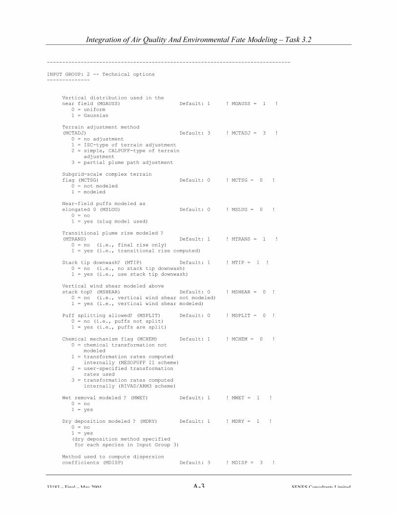
Integration of Air Quality And Environmental Fate Modeling – Task 3.2
33183 – Final – May 2004 A-3 SENES Consultants Limited
-------------------------------------------------------------------------------
INPUT GROUP: 2 -- Technical options
--------------
Vertical distribution used in the
near field (MGAUSS) Default: 1 ! MGAUSS = 1 !
0 = uniform
1 = Gaussian
Terrain adjustment method
(MCTADJ) Default: 3 ! MCTADJ = 3 !
0 = no adjustment
1 = ISC-type of terrain adjustment
2 = simple, CALPUFF-type of terrain
adjustment
3 = partial plume path adjustment
Subgrid-scale complex terrain
flag (MCTSG) Default: 0 ! MCTSG = 0 !
0 = not modeled
1 = modeled
Near-field puffs modeled as
elongated 0 (MSLUG) Default: 0 ! MSLUG = 0 !
0 = no
1 = yes (slug model used)
Transitional plume rise modeled ?
(MTRANS) Default: 1 ! MTRANS = 1 !
0 = no (i.e., final rise only)
1 = yes (i.e., transitional rise computed)
Stack tip downwash? (MTIP) Default: 1 ! MTIP = 1 !
0 = no (i.e., no stack tip downwash)
1 = yes (i.e., use stack tip downwash)
Vertical wind shear modeled above
stack top? (MSHEAR) Default: 0 ! MSHEAR = 0 !
0 = no (i.e., vertical wind shear not modeled)
1 = yes (i.e., vertical wind shear modeled)
Puff splitting allowed? (MSPLIT) Default: 0 ! MSPLIT = 0 !
0 = no (i.e., puffs not split)
1 = yes (i.e., puffs are split)
Chemical mechanism flag (MCHEM) Default: 1 ! MCHEM = 0 !
0 = chemical transformation not
modeled
1 = transformation rates computed
internally (MESOPUFF II scheme)
2 = user-specified transformation
rates used
3 = transformation rates computed
internally (RIVAD/ARM3 scheme)
Wet removal modeled ? (MWET) Default: 1 ! MWET = 1 !
0 = no
1 = yes
Dry deposition modeled ? (MDRY) Default: 1 ! MDRY = 1 !
0 = no
1 = yes
(dry deposition method specified
for each species in Input Group 3)
Method used to compute dispersion
coefficients (MDISP) Default: 3 ! MDISP = 3 !

Integration of Air Quality And Environmental Fate Modeling – Task 3.2
33183 – Final – May 2004 A-4 SENES Consultants Limited
1 = dispersion coefficients computed from measured values
of turbulence, sigma v, sigma w
2 = dispersion coefficients from internally calculated
sigma v, sigma w using micrometeorological variables
(u*, w*, L, etc.)
3 = PG dispersion coefficients for RURAL areas (computed using
the ISCST multi-segment approximation) and MP coefficients in
urban areas
4 = same as 3 except PG coefficients computed using
the MESOPUFF II eqns.
5 = CTDM sigmas used for stable and neutral conditions.
For unstable conditions, sigmas are computed as in
MDISP = 3, described above. MDISP = 5 assumes that
measured values are read
Sigma-v/sigma-theta, sigma-w measurements used? (MTURBVW)
(Used only if MDISP = 1 or 5) Default: 3 ! MTURBVW = 3 !
1 = use sigma-v or sigma-theta measurements
from PROFILE.DAT to compute sigma-y
(valid for METFM = 1, 2, 3, 4)
2 = use sigma-w measurements
from PROFILE.DAT to compute sigma-z
(valid for METFM = 1, 2, 3, 4)
3 = use both sigma-(v/theta) and sigma-w
from PROFILE.DAT to compute sigma-y and sigma-z
(valid for METFM = 1, 2, 3, 4)
4 = use sigma-theta measurements
from PLMMET.DAT to compute sigma-y
(valid only if METFM = 3)
Back-up method used to compute dispersion
when measured turbulence data are
missing (MDISP2) Default: 3 ! MDISP2 = 3 !
(used only if MDISP = 1 or 5)
2 = dispersion coefficients from internally calculated
sigma v, sigma w using micrometeorological variables
(u*, w*, L, etc.)
3 = PG dispersion coefficients for RURAL areas (computed using
the ISCST multi-segment approximation) and MP coefficients in
urban areas
4 = same as 3 except PG coefficients computed using
the MESOPUFF II eqns.
PG sigma-y,z adj. for roughness? Default: 0 ! MROUGH = 0 !
(MROUGH)
0 = no
1 = yes
Partial plume penetration of Default: 1 ! MPARTL = 1 !
elevated inversion?
(MPARTL)
0 = no
1 = yes
Strength of temperature inversion Default: 0 ! MTINV = 0 !
provided in PROFILE.DAT extended records?
(MTINV)
0 = no (computed from measured/default gradients)
1 = yes
PDF used for dispersion under convective conditions?
Default: 0 ! MPDF = 0 !
(MPDF)
0 = no
1 = yes
Sub-Grid TIBL module used for shore line?
Default: 0 ! MSGTIBL = 0 !
(MSGTIBL)

Integration of Air Quality And Environmental Fate Modeling – Task 3.2
33183 – Final – May 2004 A-5 SENES Consultants Limited
0 = no
1 = yes
Test options specified to see if
they conform to regulatory
values? (MREG) Default: 1 ! MREG = 0 !
0 = NO checks are made
1 = Technical options must conform to USEPA values
METFM 1
AVET 60. (min)
MGAUSS 1
MCTADJ 3
MTRANS 1
MTIP 1
MCHEM 1 (if modeling SOx, NOx)
MWET 1
MDRY 1
MDISP 3
MROUGH 0
MPARTL 1
SYTDEP 550. (m)
MHFTSZ 0
!END!
-------------------------------------------------------------------------------
INPUT GROUP: 3a, 3b -- Species list
-------------------
------------
Subgroup (3a)
------------
The following species are modeled:
! CSPEC = SO2 ! !END!
Dry OUTPUT GROUP
SPECIES MODELED EMITTED DEPOSITED NUMBER
NAME (0=NO, 1=YES) (0=NO, 1=YES) (0=NO, (0=NONE,
(Limit: 12 1=COMPUTED-GAS 1=1st CGRUP,
Characters 2=COMPUTED-PARTICLE 2=2nd CGRUP,
in length) 3=USER-SPECIFIED) 3= etc.)
! SO2 = 1, 1, 1, 0 !
!END!
-------------
Subgroup (3b)
-------------
The following names are used for Species-Groups in which results
for certain species are combined (added) prior to output. The
CGRUP name will be used as the species name in output files.
Use this feature to model specific particle-size distributions
by treating each size-range as a separate species.
Order must be consistent with 3(a) above.
-------------------------------------------------------------------------------
INPUT GROUP: 4 -- Grid control parameters
--------------

Integration of Air Quality And Environmental Fate Modeling – Task 3.2
33183 – Final – May 2004 A-6 SENES Consultants Limited
METEOROLOGICAL grid:
No. X grid cells (NX) No default ! NX = 120 !
No. Y grid cells (NY) No default ! NY = 120 !
No. vertical layers (NZ) No default ! NZ = 10 !
Grid spacing (DGRIDKM) No default ! DGRIDKM = 5.0!
Units: km
Cell face heights
(ZFACE(nz+1)) No defaults
Units: m
! ZFACE = 0., 20., 40., 80., 160., 300., 600., 1000., 1500., 2200.,
3000. !
Reference Coordinates
of SOUTHWEST corner of
grid cell(1, 1):
X coordinate (XORIGKM) No default ! XORIGKM = 0. !
Y coordinate (YORIGKM) No default ! YORIGKM = 0. !
Units: km
UTM zone (IUTMZN) No default ! IUTMZN = 0 !
Reference coordinates of CENTER
of the domain (used in the
calculation of solar elevation
angles)
Latitude (deg.) (XLAT) No default ! XLAT = 46.000 !
Longitude (deg.) (XLONG) No default ! XLONG = 92.000 !
Time zone (XTZ) No default ! XTZ = 6.0 !
(PST=8, MST=7, CST=6, EST=5)
Computational grid:
The computational grid is identical to or a subset of the MET. grid.
The lower left (LL) corner of the computational grid is at grid point
(IBCOMP, JBCOMP) of the MET. grid. The upper right (UR) corner of the
computational grid is at grid point (IECOMP, JECOMP) of the MET. grid.
The grid spacing of the computational grid is the same as the MET. grid.
X index of LL corner (IBCOMP) No default ! IBCOMP = 1 !
(1 <= IBCOMP <= NX)
Y index of LL corner (JBCOMP) No default ! JBCOMP = 1 !
(1 <= JBCOMP <= NY)
X index of UR corner (IECOMP) No default ! IECOMP = 120 !
(1 <= IECOMP <= NX)
Y index of UR corner (JECOMP) No default ! JECOMP = 120 !
(1 <= JECOMP <= NY)
SAMPLING GRID (GRIDDED RECEPTORS):
The lower left (LL) corner of the sampling grid is at grid point
(IBSAMP, JBSAMP) of the MET. grid. The upper right (UR) corner of the
sampling grid is at grid point (IESAMP, JESAMP) of the MET. grid.
The sampling grid must be identical to or a subset of the computational
grid. It may be a nested grid inside the computational grid.
The grid spacing of the sampling grid is DGRIDKM/MESHDN.

Integration of Air Quality And Environmental Fate Modeling – Task 3.2
33183 – Final – May 2004 A-7 SENES Consultants Limited
Logical flag indicating if gridded
receptors are used (LSAMP) Default: T ! LSAMP = T !
(T=yes, F=no)
X index of LL corner (IBSAMP) No default ! IBSAMP = 1 !
(IBCOMP <= IBSAMP <= IECOMP)
Y index of LL corner (JBSAMP) No default ! JBSAMP = 1 !
(JBCOMP <= JBSAMP <= JECOMP)
X index of UR corner (IESAMP) No default ! IESAMP = 120 !
(IBCOMP <= IESAMP <= IECOMP)
Y index of UR corner (JESAMP) No default ! JESAMP = 120 !
(JBCOMP <= JESAMP <= JECOMP)
Nesting factor of the sampling
grid (MESHDN) Default: 1 ! MESHDN = 1 !
(MESHDN is an integer >= 1)
!END!
-------------------------------------------------------------------------------
INPUT GROUP: 5 -- Output Options
--------------
* *
FILE DEFAULT VALUE VALUE THIS RUN
---- ------------- --------------
Concentrations (ICON) 1 ! ICON = 1 !
Dry Fluxes (IDRY) 1 ! IDRY = 1 !
Wet Fluxes (IWET) 1 ! IWET = 1 !
Relative Humidity (IVIS) 1 ! IVIS = 1 !
(relative humidity file is
required for visibility
analysis)
Use data compression option in output file?
(LCOMPRS) Default: T ! LCOMPRS = T !
*
0 = Do not create file, 1 = create file
DIAGNOSTIC MASS FLUX OUTPUT OPTIONS:
Mass flux across specified boundaries
for selected species reported hourly?
(IMFLX) Default: 0 ! IMFLX = 0 !
0 = no
1 = yes (FLUXBDY.DAT and MASSFLX.DAT filenames
are specified in Input Group 0)
Mass balance for each species
reported hourly?
(IMBAL) Default: 0 ! IMBAL = 0 !
0 = no
1 = yes (MASSBAL.DAT filename is
specified in Input Group 0)
LINE PRINTER OUTPUT OPTIONS:
Print concentrations (ICPRT) Default: 0 ! ICPRT = 1 !
Print dry fluxes (IDPRT) Default: 0 ! IDPRT = 1 !
Print wet fluxes (IWPRT) Default: 0 ! IWPRT = 1 !
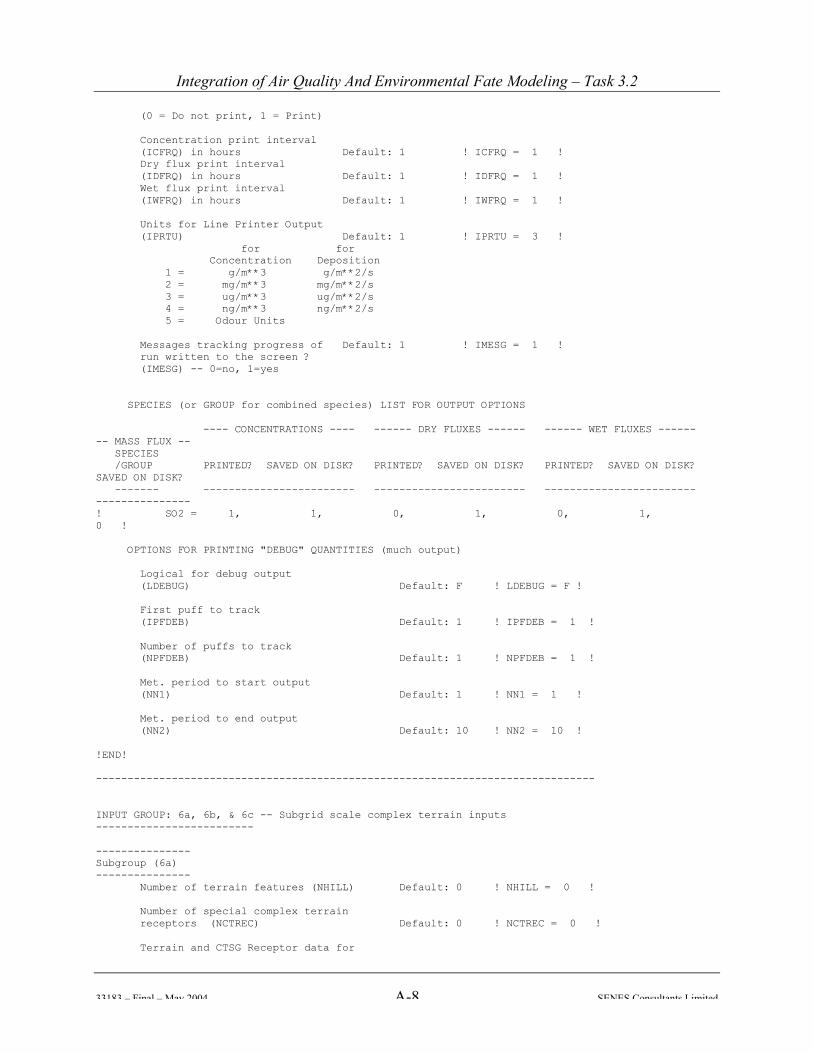
Integration of Air Quality And Environmental Fate Modeling – Task 3.2
33183 – Final – May 2004 A-8 SENES Consultants Limited
(0 = Do not print, 1 = Print)
Concentration print interval
(ICFRQ) in hours Default: 1 ! ICFRQ = 1 !
Dry flux print interval
(IDFRQ) in hours Default: 1 ! IDFRQ = 1 !
Wet flux print interval
(IWFRQ) in hours Default: 1 ! IWFRQ = 1 !
Units for Line Printer Output
(IPRTU) Default: 1 ! IPRTU = 3 !
for for
Concentration Deposition
1 = g/m**3 g/m**2/s
2 = mg/m**3 mg/m**2/s
3 = ug/m**3 ug/m**2/s
4 = ng/m**3 ng/m**2/s
5 = Odour Units
Messages tracking progress of Default: 1 ! IMESG = 1 !
run written to the screen ?
(IMESG) -- 0=no, 1=yes
SPECIES (or GROUP for combined species) LIST FOR OUTPUT OPTIONS
---- CONCENTRATIONS ---- ------ DRY FLUXES ------ ------ WET FLUXES ------
-- MASS FLUX --
SPECIES
/GROUP PRINTED? SAVED ON DISK? PRINTED? SAVED ON DISK? PRINTED? SAVED ON DISK?
SAVED ON DISK?
------- ------------------------ ------------------------ ------------------------
---------------
! SO2 = 1, 1, 0, 1, 0, 1,
0 !
OPTIONS FOR PRINTING "DEBUG" QUANTITIES (much output)
Logical for debug output
(LDEBUG) Default: F ! LDEBUG = F !
First puff to track
(IPFDEB) Default: 1 ! IPFDEB = 1 !
Number of puffs to track
(NPFDEB) Default: 1 ! NPFDEB = 1 !
Met. period to start output
(NN1) Default: 1 ! NN1 = 1 !
Met. period to end output
(NN2) Default: 10 ! NN2 = 10 !
!END!
-------------------------------------------------------------------------------
INPUT GROUP: 6a, 6b, & 6c -- Subgrid scale complex terrain inputs
-------------------------
---------------
Subgroup (6a)
---------------
Number of terrain features (NHILL) Default: 0 ! NHILL = 0 !
Number of special complex terrain
receptors (NCTREC) Default: 0 ! NCTREC = 0 !
Terrain and CTSG Receptor data for

Integration of Air Quality And Environmental Fate Modeling – Task 3.2
33183 – Final – May 2004 A-9 SENES Consultants Limited
CTSG hills input in CTDM format ?
(MHILL) No Default ! MHILL = 2 !
1 = Hill and Receptor data created
by CTDM processors & read from
HILL.DAT and HILLRCT.DAT files
2 = Hill data created by OPTHILL &
input below in Subgroup (6b);
Receptor data in Subgroup (6c)
Factor to convert horizontal dimensions Default: 1.0 ! XHILL2M = 1. !
to meters (MHILL=1)
Factor to convert vertical dimensions Default: 1.0 ! ZHILL2M = 1. !
to meters (MHILL=1)
X-origin of CTDM system relative to No Default ! XCTDMKM = 0.0E00 !
CALPUFF coordinate system, in Kilometers (MHILL=1)
Y-origin of CTDM system relative to No Default ! YCTDMKM = 0.0E00 !
CALPUFF coordinate system, in Kilometers (MHILL=1)
! END !
---------------
Subgroup (6b)
---------------
1 **
HILL information
HILL XC YC THETAH ZGRID RELIEF EXPO 1 EXPO 2 SCALE 1 SCALE 2
AMAX1 AMAX2
NO. (km) (km) (deg.) (m) (m) (m) (m) (m) (m)
(m) (m)
---- ---- ---- ------ ----- ------ ------ ------ ------- -------
----- -----
---------------
Subgroup (6c)
---------------
COMPLEX TERRAIN RECEPTOR INFORMATION
XRCT YRCT ZRCT XHH
(km) (km) (m)
------ ----- ------ ----
-------------------
1
Description of Complex Terrain Variables:
XC, YC = Coordinates of center of hill
THETAH = Orientation of major axis of hill (clockwise from
North)
ZGRID = Height of the 0 of the grid above mean sea
level
RELIEF = Height of the crest of the hill above the grid elevation
EXPO 1 = Hill-shape exponent for the major axis
EXPO 2 = Hill-shape exponent for the major axis
SCALE 1 = Horizontal length scale along the major axis
SCALE 2 = Horizontal length scale along the minor axis
AMAX = Maximum allowed axis length for the major axis
BMAX = Maximum allowed axis length for the major axis
XRCT, YRCT = Coordinates of the complex terrain receptors
ZRCT = Height of the ground (MSL) at the complex terrain
Receptor
XHH = Hill number associated with each complex terrain receptor
(NOTE: MUST BE ENTERED AS A REAL NUMBER)
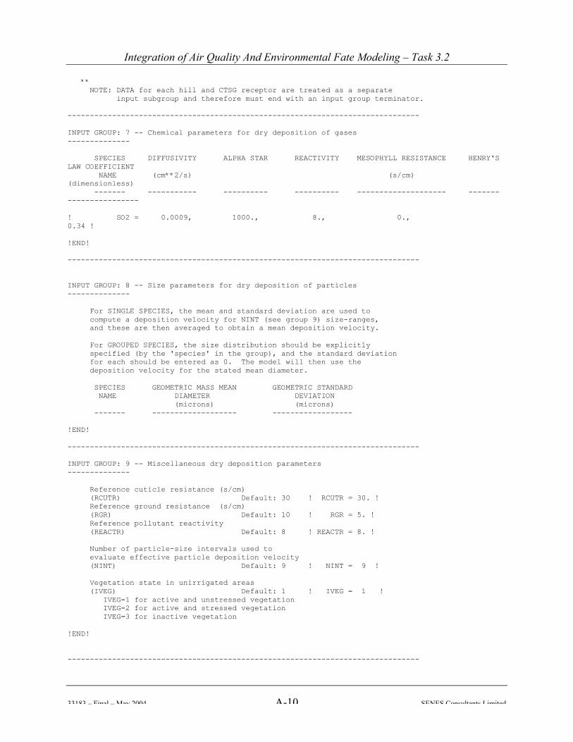
Integration of Air Quality And Environmental Fate Modeling – Task 3.2
33183 – Final – May 2004 A-10 SENES Consultants Limited
**
NOTE: DATA for each hill and CTSG receptor are treated as a separate
input subgroup and therefore must end with an input group terminator.
-------------------------------------------------------------------------------
INPUT GROUP: 7 -- Chemical parameters for dry deposition of gases
--------------
SPECIES DIFFUSIVITY ALPHA STAR REACTIVITY MESOPHYLL RESISTANCE HENRY'S
LAW COEFFICIENT
NAME (cm**2/s) (s/cm)
(dimensionless)
------- ----------- ---------- ---------- -------------------- -------
----------------
! SO2 = 0.0009, 1000., 8., 0.,
0.34 !
!END!
-------------------------------------------------------------------------------
INPUT GROUP: 8 -- Size parameters for dry deposition of particles
--------------
For SINGLE SPECIES, the mean and standard deviation are used to
compute a deposition velocity for NINT (see group 9) size-ranges,
and these are then averaged to obtain a mean deposition velocity.
For GROUPED SPECIES, the size distribution should be explicitly
specified (by the 'species' in the group), and the standard deviation
for each should be entered as 0. The model will then use the
deposition velocity for the stated mean diameter.
SPECIES GEOMETRIC MASS MEAN GEOMETRIC STANDARD
NAME DIAMETER DEVIATION
(microns) (microns)
------- ------------------- ------------------
!END!
-------------------------------------------------------------------------------
INPUT GROUP: 9 -- Miscellaneous dry deposition parameters
--------------
Reference cuticle resistance (s/cm)
(RCUTR) Default: 30 ! RCUTR = 30. !
Reference ground resistance (s/cm)
(RGR) Default: 10 ! RGR = 5. !
Reference pollutant reactivity
(REACTR) Default: 8 ! REACTR = 8. !
Number of particle-size intervals used to
evaluate effective particle deposition velocity
(NINT) Default: 9 ! NINT = 9 !
Vegetation state in unirrigated areas
(IVEG) Default: 1 ! IVEG = 1 !
IVEG=1 for active and unstressed vegetation
IVEG=2 for active and stressed vegetation
IVEG=3 for inactive vegetation
!END!
-------------------------------------------------------------------------------

Integration of Air Quality And Environmental Fate Modeling – Task 3.2
33183 – Final – May 2004 A-11 SENES Consultants Limited
INPUT GROUP: 10 -- Wet Deposition Parameters
---------------
Scavenging Coefficient -- Units: (sec)**(-1)
Pollutant Liquid Precip. Frozen Precip.
--------- -------------- --------------
! SO2 = 3.0E-05, 0.0E00 !
!END!
-------------------------------------------------------------------------------
INPUT GROUP: 11 -- Chemistry Parameters
---------------
Ozone data input option (MOZ) Default: 1 ! MOZ = 1 !
(Used only if MCHEM = 1 or 3)
0 = use a constant background ozone value
1 = read hourly ozone concentrations from
the OZONE.DAT data file
Background ozone concentration
(BCKO3) in ppb Default: 80. ! BCKO3 = 40. !
(Used only if MCHEM = 1 or 3 and
MOZ = 0 or (MOZ = 1 and all hourly
O3 data missing)
Background ammonia concentration
(BCKNH3) in ppb Default: 10. ! BCKNH3 = 10. !
Nighttime SO2 loss rate (RNITE1)
in percent/hour Default: 0.2 ! RNITE1 = 0.2 !
Nighttime NOx loss rate (RNITE2)
in percent/hour Default: 2.0 ! RNITE2 = 2. !
Nighttime HNO3 formation rate (RNITE3)
in percent/hour Default: 2.0 ! RNITE3 = 2. !
!END!
-------------------------------------------------------------------------------
INPUT GROUP: 12 -- Misc. Dispersion and Computational Parameters
---------------
Horizontal size of puff (m) beyond which
time-dependent dispersion equations (Heffter)
are used to determine sigma-y and
sigma-z (SYTDEP) Default: 550. ! SYTDEP = 5.5E02 !
Switch for using Heffter equation for sigma z
as above (0 = Not use Heffter; 1 = use Heffter
(MHFTSZ) Default: 0 ! MHFTSZ = 0 !
Stability class used to determine plume
growth rates for puffs above the boundary
layer (JSUP) Default: 5 ! JSUP = 5 !
Vertical dispersion constant for stable
conditions (k1 in Eqn. 2.7-3) (CONK1) Default: 0.01 ! CONK1 = 0.01 !
Vertical dispersion constant for neutral/

Integration of Air Quality And Environmental Fate Modeling – Task 3.2
33183 – Final – May 2004 A-12 SENES Consultants Limited
unstable conditions (k2 in Eqn. 2.7-4)
(CONK2) Default: 0.1 ! CONK2 = 0.1 !
Factor for determining Transition-point from
Schulman-Scire to Huber-Snyder Building Downwash
scheme (SS used for Hs < Hb + TBD * HL)
(TBD) Default: 0.5 ! TBD = 0.5 !
TBD < 0 ==> always use Huber-Snyder
TBD = 1.5 ==> always use Schulman-Scire
TBD = 0.5 ==> ISC Transition-point
Range of land use categories for which
urban dispersion is assumed
(IURB1, IURB2) Default: 10 ! IURB1 = 10 !
19 ! IURB2 = 19 !
Site characterization parameters for single-point Met data files ---------
(needed for METFM = 2,3,4)
Land use category for modeling domain
(ILANDUIN) Default: 20 ! ILANDUIN = 20 !
Roughness length (m) for modeling domain
(Z0IN) Default: 0.25 ! Z0IN = 0.25 !
Leaf area index for modeling domain
(XLAIIN) Default: 3.0 ! XLAIIN = 3. !
Elevation above sea level (m)
(ELEVIN) Default: 0.0 ! ELEVIN = 0. !
Latitude (degrees) for met location
(XLATIN) Default: -999. ! XLATIN = 0. !
Longitude (degrees) for met location
(XLONIN) Default: -999. ! XLONIN = 0. !
Specialized information for interpreting single-point Met data files -----
Anemometer height (m) (Used only if METFM = 2,3)
(ANEMHT) Default: 10. ! ANEMHT = 10. !
Form of lateral turbulance data in PROFILE.DAT file
(Used only if METFM = 4 or MTURBVW = 1 or 3)
(ISIGMAV) Default: 1 ! ISIGMAV = 1 !
0 = read sigma-theta
1 = read sigma-v
Choice of mixing heights (Used only if METFM = 4)
(IMIXCTDM) Default: 0 ! IMIXCTDM = 0 !
0 = read PREDICTED mixing heights
1 = read OBSERVED mixing heights
Maximum length of a slug (met. grid units)
(XMXLEN) Default: 1.0 ! XMXLEN = 1. !
Maximum travel distance of a puff/slug (in
grid units) during one sampling step
(XSAMLEN) Default: 1.0 ! XSAMLEN = 1. !
Maximum Number of slugs/puffs release from
one source during one time step
(MXNEW) Default: 99 ! MXNEW = 99 !
Maximum Number of sampling steps for
one puff/slug during one time step
(MXSAM) Default: 99 ! MXSAM = 99 !
Number of iterations used when computing
the transport wind for a sampling step

Integration of Air Quality And Environmental Fate Modeling – Task 3.2
33183 – Final – May 2004 A-13 SENES Consultants Limited
that includes gradual rise (for CALMET
and PROFILE winds)
(NCOUNT) Default: 2 ! NCOUNT = 2 !
Minimum sigma y for a new puff/slug (m)
(SYMIN) Default: 1.0 ! SYMIN = 1. !
Minimum sigma z for a new puff/slug (m)
(SZMIN) Default: 1.0 ! SZMIN = 1. !
Default minimum turbulence velocities
sigma-v and sigma-w for each
stability class (m/s)
(SVMIN(6) and SWMIN(6)) Default SVMIN : .50, .50, .50, .50, .50, .50
Default SWMIN : .20, .12, .08, .06, .03, .016
Stability Class : A B C D E F
--- --- --- --- --- ---
! SVMIN = 0.500, 0.500, 0.500, 0.500, 0.500, 0.500!
! SWMIN = 0.200, 0.120, 0.080, 0.060, 0.030, 0.016!
Divergence criterion for dw/dz across puff
used to initiate adjustment for horizontal
convergence (1/s)
Partial adjustment starts at CDIV(1), and
full adjustment is reached at CDIV(2)
(CDIV(2)) Default: 0.0,0.0 ! CDIV = 0., 0. !
Minimum wind speed (m/s) allowed for
non-calm conditions. Also used as minimum
speed returned when using power-law
extrapolation toward surface
(WSCALM) Default: 0.5 ! WSCALM = 0.5 !
Maximum mixing height (m)
(XMAXZI) Default: 3000. ! XMAXZI = 3000. !
Minimum mixing height (m)
(XMINZI) Default: 50. ! XMINZI = 20. !
Default wind speed classes --
5 upper bounds (m/s) are entered;
the 6th class has no upper limit
(WSCAT(5)) Default :
ISC RURAL : 1.54, 3.09, 5.14, 8.23, 10,8 (10.8+)
Wind Speed Class : 1 2 3 4 5 6
--- --- --- --- --- ---
! WSCAT = 1.54, 3.09, 5.14, 8.23, 10.80 !
Default wind speed profile power-law
exponents for stabilities 1-6
(PLX0(6)) Default : ISC RURAL values
ISC RURAL : .07, .07, .10, .15, .35, .55
ISC URBAN : .15, .15, .20, .25, .30, .30
Stability Class : A B C D E F
--- --- --- --- --- ---
! PLX0 = 0.07, 0.07, 0.10, 0.15, 0.35, 0.55 !
Default potential temperature gradient
for stable classes E, F (degK/m)
(PTG0(2)) Default: 0.020, 0.035
! PTG0 = 0.020, 0.035 !
Default plume path coefficients for
each stability class (used when option
for partial plume height terrain adjustment
is selected -- MCTADJ=3)
(PPC(6)) Stability Class : A B C D E F

Integration of Air Quality And Environmental Fate Modeling – Task 3.2
33183 – Final – May 2004 A-14 SENES Consultants Limited
Default PPC : .50, .50, .50, .50, .35, .35
--- --- --- --- --- ---
! PPC = 0.50, 0.50, 0.50, 0.50, 0.35, 0.35 !
Slug-to-puff transition criterion factor
equal to sigma-y/length of slug
(SL2PF) Default: 10. ! SL2PF = 10. !
Puff-splitting control variables ------------------------
Number of puffs that result every time a puff
is split - nsplit=2 means that 1 puff splits
into 2
(NSPLIT) Default: 3 ! NSPLIT = 3 !
Time(s) of a day when split puffs are eligible to
be split once again; this is typically set once
per day, around sunset before nocturnal shear develops.
24 values: 0 is midnight (00:00) and 23 is 11 PM (23:00)
0=do not re-split 1=eligible for re-split
(IRESPLIT(24)) Default: Hour 17 = 1
! IRESPLIT = 0,0,0,0,0,0,0,0,0,0,0,0,0,0,0,0,0,1,0,0,0,0,0,0 !
Split is allowed only if last hour's mixing
height (m) exceeds a minimum value
(ZISPLIT) Default: 100. ! ZISPLIT = 100. !
Split is allowed only if ratio of last hour's
mixing ht to the maximum mixing ht experienced
by the puff is less than a maximum value (this
postpones a split until a nocturnal layer develops)
(ROLDMAX) Default: 0.25 ! ROLDMAX = 0.25 !
Integration control variables ------------------------
Fractional convergence criterion for numerical SLUG
sampling integration
(EPSSLUG) Default: 1.0e-04 ! EPSSLUG = 1.0E-04 !
Fractional convergence criterion for numerical AREA
source integration
(EPSAREA) Default: 1.0e-06 ! EPSAREA = 1.0E-06 !
Trajectory step-length (m) used for numerical rise
integration
(DSRISE) Default: 1.0 ! DSRISE = 1. !
!END!
-------------------------------------------------------------------------------
INPUT GROUPS: 13a, 13b, 13c, 13d -- Point source parameters
--------------------------------
---------------
Subgroup (13a)
---------------
Number of point sources with
parameters provided below (NPT1) No default ! NPT1 = 92 !
Units used for point source
emissions below (IPTU) Default: 1 ! IPTU = 1 !
1 = g/s
2 = kg/hr
3 = lb/hr
4 = tons/yr
5 = Odour Unit * m**3/s (vol. flux of odour compound)

Integration of Air Quality And Environmental Fate Modeling – Task 3.2
33183 – Final – May 2004 A-15 SENES Consultants Limited
6 = Odour Unit * m**3/min
7 = metric tons/yr
Number of source-species
combinations with variable
emissions scaling factors
provided below in (13d) (NSPT1) Default: 0 ! NSPT1 = 0 !
Number of point sources with
variable emission parameters
provided in external file (NPT2) No default ! NPT2 = 0 !
(If NPT2 > 0, these point
source emissions are read from
the file: PTEMARB.DAT)
!END!
---------------
Subgroup (13b)
---------------
a
POINT SOURCE: CONSTANT DATA
-----------------------------
b c
Source X UTM Y UTM Stack Base Stack Exit Exit Bldg. Emission
No. Coordinate Coordinate Height Elevation Diameter Vel. Temp. Dwash Rates
(km) (km) (m) (m) (m) (m/s) (deg. K)
------ ---------- ---------- ------ ------ -------- ----- -------- ----- --------
1 ! SRCNAM = STK1 !
1 ! X = 268.860, 150.589, 23.698, 253.17, 2.40, 20.00, 337.85, .0, 1.02E+00
!!END!
2 ! SRCNAM = STK2 !
2 ! X = 234.770, 218.717, 8.598, 301.97, 0.87, 11.00, 300.85, .0, 3.16E-01
!!END!
3 ! SRCNAM = STK3 !
3 ! X = 281.586, 135.161, 38.499, 267.57, 1.11, 27.00, 406.85, .0, 2.39E-01
!!END!
4 ! SRCNAM = STK4 !
4 ! X = 260.939, 105.762, 15.700, 322.93, 0.90, 12.00, 418.85, .0, 2.22E-01
!!END!
5 ! SRCNAM = STK5 !
5 ! X = 268.860, 150.589, 10.000, 253.17, 1.00, 1.00, 293.00, .0, 2.16E-01
!!END!
6 ! SRCNAM = STK6 !
6 ! X = 234.770, 218.717, 8.598, 301.97, 0.87, 11.00, 300.85, .0, 1.93E-01
!!END!
7 ! SRCNAM = STK7 !
7 ! X = 283.843, 147.304, 6.200, 254.01, 0.28, 10.00, 290.85, .0, 1.71E-01
!!END!
8 ! SRCNAM = STK8 !
8 ! X = 231.021, 136.797, 8.598, 295.03, 0.87, 11.00, 300.85, .0, 1.51E-01
!!END!
9 ! SRCNAM = STK9 !
9 ! X = 265.775, 170.335, 9.598, 273.59, 2.60, 20.00, 294.85, .0, 1.35E-01
!!END!
10 ! SRCNAM = STK10!
10 ! X = 283.452, 144.176, 38.499, 249.83, 1.11, 27.00, 406.85, .0, 1.07E-01
!!END!
11 ! SRCNAM = STK11 !
11 ! X = 300.271, 163.250, 7.800, 256.24, 0.55, 12.00, 299.85, .0, 8.20E-02
!!END!
12 ! SRCNAM = STK12 !
12 ! X = 265.606, 84.680, 15.700, 322.67, 0.90, 12.00, 418.85, .0, 5.58E-02
!!END!
13 ! SRCNAM = STK13 !
13 ! X = 325.462, 60.242, 10.000, 327.09, 1.00, 1.00, 293.00, .0, 4.23E-02
!!END!
14 ! SRCNAM = STK14 !
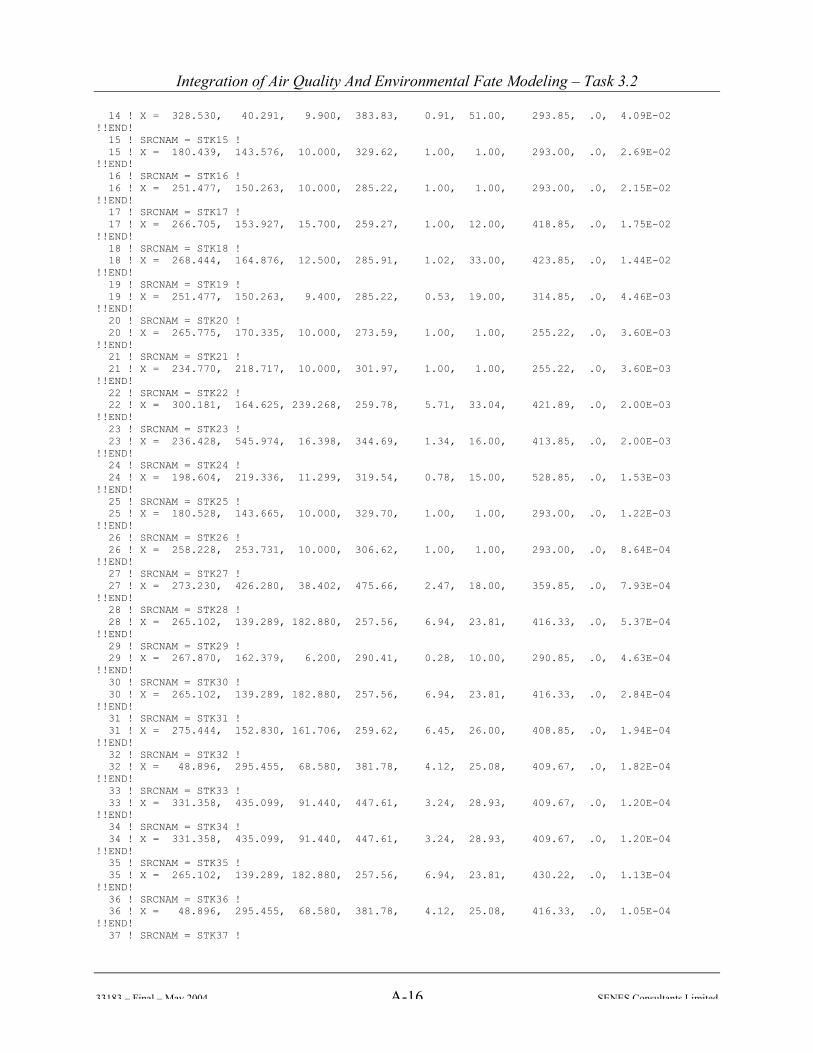
Integration of Air Quality And Environmental Fate Modeling – Task 3.2
33183 – Final – May 2004 A-16 SENES Consultants Limited
14 ! X = 328.530, 40.291, 9.900, 383.83, 0.91, 51.00, 293.85, .0, 4.09E-02
!!END!
15 ! SRCNAM = STK15 !
15 ! X = 180.439, 143.576, 10.000, 329.62, 1.00, 1.00, 293.00, .0, 2.69E-02
!!END!
16 ! SRCNAM = STK16 !
16 ! X = 251.477, 150.263, 10.000, 285.22, 1.00, 1.00, 293.00, .0, 2.15E-02
!!END!
17 ! SRCNAM = STK17 !
17 ! X = 266.705, 153.927, 15.700, 259.27, 1.00, 12.00, 418.85, .0, 1.75E-02
!!END!
18 ! SRCNAM = STK18 !
18 ! X = 268.444, 164.876, 12.500, 285.91, 1.02, 33.00, 423.85, .0, 1.44E-02
!!END!
19 ! SRCNAM = STK19 !
19 ! X = 251.477, 150.263, 9.400, 285.22, 0.53, 19.00, 314.85, .0, 4.46E-03
!!END!
20 ! SRCNAM = STK20 !
20 ! X = 265.775, 170.335, 10.000, 273.59, 1.00, 1.00, 255.22, .0, 3.60E-03
!!END!
21 ! SRCNAM = STK21 !
21 ! X = 234.770, 218.717, 10.000, 301.97, 1.00, 1.00, 255.22, .0, 3.60E-03
!!END!
22 ! SRCNAM = STK22 !
22 ! X = 300.181, 164.625, 239.268, 259.78, 5.71, 33.04, 421.89, .0, 2.00E-03
!!END!
23 ! SRCNAM = STK23 !
23 ! X = 236.428, 545.974, 16.398, 344.69, 1.34, 16.00, 413.85, .0, 2.00E-03
!!END!
24 ! SRCNAM = STK24 !
24 ! X = 198.604, 219.336, 11.299, 319.54, 0.78, 15.00, 528.85, .0, 1.53E-03
!!END!
25 ! SRCNAM = STK25 !
25 ! X = 180.528, 143.665, 10.000, 329.70, 1.00, 1.00, 293.00, .0, 1.22E-03
!!END!
26 ! SRCNAM = STK26 !
26 ! X = 258.228, 253.731, 10.000, 306.62, 1.00, 1.00, 293.00, .0, 8.64E-04
!!END!
27 ! SRCNAM = STK27 !
27 ! X = 273.230, 426.280, 38.402, 475.66, 2.47, 18.00, 359.85, .0, 7.93E-04
!!END!
28 ! SRCNAM = STK28 !
28 ! X = 265.102, 139.289, 182.880, 257.56, 6.94, 23.81, 416.33, .0, 5.37E-04
!!END!
29 ! SRCNAM = STK29 !
29 ! X = 267.870, 162.379, 6.200, 290.41, 0.28, 10.00, 290.85, .0, 4.63E-04
!!END!
30 ! SRCNAM = STK30 !
30 ! X = 265.102, 139.289, 182.880, 257.56, 6.94, 23.81, 416.33, .0, 2.84E-04
!!END!
31 ! SRCNAM = STK31 !
31 ! X = 275.444, 152.830, 161.706, 259.62, 6.45, 26.00, 408.85, .0, 1.94E-04
!!END!
32 ! SRCNAM = STK32 !
32 ! X = 48.896, 295.455, 68.580, 381.78, 4.12, 25.08, 409.67, .0, 1.82E-04
!!END!
33 ! SRCNAM = STK33 !
33 ! X = 331.358, 435.099, 91.440, 447.61, 3.24, 28.93, 409.67, .0, 1.20E-04
!!END!
34 ! SRCNAM = STK34 !
34 ! X = 331.358, 435.099, 91.440, 447.61, 3.24, 28.93, 409.67, .0, 1.20E-04
!!END!
35 ! SRCNAM = STK35 !
35 ! X = 265.102, 139.289, 182.880, 257.56, 6.94, 23.81, 430.22, .0, 1.13E-04
!!END!
36 ! SRCNAM = STK36 !
36 ! X = 48.896, 295.455, 68.580, 381.78, 4.12, 25.08, 416.33, .0, 1.05E-04
!!END!
37 ! SRCNAM = STK37 !

Integration of Air Quality And Environmental Fate Modeling – Task 3.2
33183 – Final – May 2004 A-17 SENES Consultants Limited
37 ! X = 265.102, 139.289, 182.880, 257.56, 6.94, 23.81, 409.67, .0, 6.43E-05
!!END!
38 ! SRCNAM = STK38 !
38 ! X = 92.156, 133.267, 153.010, 292.47, 5.47, 25.45, 416.33, .0, 6.29E-05
!!END!
39 ! SRCNAM = STK39 !
39 ! X = 329.859, 58.330, 137.160, 322.86, 5.24, 23.16, 413.56, .0, 6.12E-05
!!END!
40 ! SRCNAM = STK40 !
40 ! X = 292.781, 21.244, 137.160, 373.64, 5.24, 23.16, 413.56, .0, 6.09E-05
!!END!
41 ! SRCNAM = STK41 !
41 ! X = 301.913, 470.365, 153.010, 415.57, 5.47, 25.45, 416.33, .0, 5.38E-05
!!END!
42 ! SRCNAM = STK42 !
42 ! X = 131.187, 172.463, 153.010, 360.57, 5.47, 25.45, 416.33, .0, 4.73E-05
!!END!
43 ! SRCNAM = STK43 !
43 ! X = 190.043, 223.403, 10.000, 322.75, 1.00, 1.00, 293.00, .0, 4.00E-05
!!END!
44 ! SRCNAM = STK44 !
44 ! X = 316.547, 347.364, 10.000, 370.97, 1.00, 1.00, 293.00, .0, 3.88E-05
!!END!
45 ! SRCNAM = STK45 !
45 ! X = 115.896, 132.628, 50.292, 323.22, 2.78, 10.72, 449.67, .0, 3.51E-05
!!END!
46 ! SRCNAM = STK46 !
46 ! X = 190.043, 223.403, 10.000, 322.75, 1.00, 0.00, 255.22, .0, 3.25E-05
!!END!
47 ! SRCNAM = STK47 !
47 ! X = 275.986, 421.296, 153.010, 449.15, 5.47, 25.45, 416.33, .0, 2.81E-05
!!END!
48 ! SRCNAM = STK48 !
48 ! X = 316.547, 347.364, 10.000, 370.97, 1.00, 1.00, 293.00, .0, 2.74E-05
!!END!
49 ! SRCNAM = STK49 !
49 ! X = 233.561, 398.238, 50.292, 396.98, 2.02, 13.66, 458.56, .0, 2.49E-05
!!END!
50 ! SRCNAM = STK50 !
50 ! X = 233.561, 398.238, 50.292, 396.98, 2.02, 13.66, 458.56, .0, 2.46E-05
!!END!
51 ! SRCNAM = STK51 !
51 ! X = 157.429, 13.295, 43.282, 381.02, 2.46, 21.66, 413.56, .0, 2.43E-05
!!END!
52 ! SRCNAM = STK52 !
52 ! X = 233.561, 398.238, 16.398, 396.98, 1.34, 16.00, 413.85, .0, 2.42E-05
!!END!
53 ! SRCNAM = STK53 !
53 ! X = 233.561, 398.238, 16.398, 396.98, 1.34, 16.00, 413.85, .0, 2.42E-05
!!END!
54 ! SRCNAM = STK54 !
54 ! X = 316.547, 347.364, 10.000, 370.97, 1.00, 1.00, 293.00, .0, 2.41E-05
!!END!
55 ! SRCNAM = STK55 !
55 ! X = 275.986, 421.296, 153.010, 449.15, 5.47, 25.45, 416.33, .0, 2.39E-05
!!END!
56 ! SRCNAM = STK56 !
56 ! X = 316.547, 347.364, 10.000, 370.97, 1.00, 1.00, 293.00, .0, 2.30E-05
!!END!
57 ! SRCNAM = STK57 !
57 ! X = 1.603, 468.195, 50.292, 400.00, 2.02, 13.66, 458.56, .0, 2.27E-05
!!END!
58 ! SRCNAM = STK58 !
58 ! X = 233.561, 398.238, 16.398, 396.98, 1.34, 16.00, 413.85, .0, 2.20E-05
!!END!
59 ! SRCNAM = STK59 !
59 ! X = 233.561, 398.238, 16.398, 396.98, 1.34, 16.00, 413.85, .0, 2.20E-05
!!END!
60 ! SRCNAM = STK60 !

Integration of Air Quality And Environmental Fate Modeling – Task 3.2
33183 – Final – May 2004 A-18 SENES Consultants Limited
60 ! X = 1.603, 468.195, 50.292, 400.00, 2.02, 13.66, 458.56, .0, 2.07E-05
!!END!
61 ! SRCNAM = STK61 !
61 ! X = 275.986, 421.296, 153.010, 449.15, 5.47, 25.45, 416.33, .0, 1.68E-05
!!END!
62 ! SRCNAM = STK62 !
62 ! X = 316.525, 347.172, 16.398, 369.83, 1.34, 16.00, 413.85, .0, 1.64E-05
!!END!
63 ! SRCNAM = STK63 !
63 ! X = 210.849, 70.345, 10.000, 281.03, 1.00, 1.00, 293.00, .0, 1.44E-05
!!END!
64 ! SRCNAM = STK64 !
64 ! X = 336.864, 349.867, 100.889, 228.16, 4.32, 9.80, 455.22, .0, 1.29E-05
!!END!
65 ! SRCNAM = STK65 !
65 ! X = 336.864, 349.867, 100.889, 228.16, 4.32, 9.80, 455.22, .0, 1.01E-05
!!END!
66 ! SRCNAM = STK66 !
66 ! X = 189.030, 304.887, 38.710, 369.17, 1.85, 10.72, 464.11, .0, 9.66E-06
!!END!
67 ! SRCNAM = STK67 !
67 ! X = 189.030, 304.887, 38.710, 369.17, 1.85, 10.72, 464.11, .0, 9.46E-06
!!END!
68 ! SRCNAM = STK68 !
68 ! X = 32.646, 97.700, 28.651, 521.80, 1.46, 11.34, 470.22, .0, 8.28E-06
!!END!
69 ! SRCNAM = STK69 !
69 ! X = 32.646, 97.700, 28.651, 521.80, 1.46, 11.34, 470.22, .0, 8.28E-06
!!END!
70 ! SRCNAM = STK70 !
70 ! X = 277.058, 156.270, 50.292, 260.47, 2.02, 13.66, 458.56, .0, 7.91E-06
!!END!
71 ! SRCNAM = STK71 !
71 ! X = 329.859, 58.330, 137.160, 322.86, 5.24, 23.16, 413.56, .0, 6.87E-06
!!END!
72 ! SRCNAM = STK72 !
72 ! X = 291.099, 138.295, 10.000, 239.75, 1.00, 1.00, 293.00, .0, 6.41E-06
!!END!
73 ! SRCNAM = STK73 !
73 ! X = 261.066, 14.992, 55.169, 376.99, 2.78, 10.72, 449.67, .0, 6.10E-06
!!END!
74 ! SRCNAM = STK74 !
74 ! X = 291.099, 138.295, 10.000, 239.75, 1.00, 1.00, 293.00, .0, 4.72E-06
!!END!
75 ! SRCNAM = STK75 !
75 ! X = 190.043, 223.403, 10.000, 322.75, 1.00, 1.00, 293.00, .0, 3.91E-06
!!END!
76 ! SRCNAM = STK76 !
76 ! X = 313.632, 347.507, 55.169, 381.11, 2.78, 10.72, 449.67, .0, 2.70E-06
!!END!
77 ! SRCNAM = STK77 !
77 ! X = 277.058, 156.270, 38.710, 260.47, 1.85, 10.72, 464.11, .0, 2.26E-06
!!END!
78 ! SRCNAM = STK78 !
78 ! X = 174.885, 82.798, 137.160, 280.30, 5.24, 23.16, 413.56, .0, 2.04E-06
!!END!
79 ! SRCNAM = STK79 !
79 ! X = 301.913, 470.365, 153.010, 415.57, 5.47, 25.45, 416.33, .0, 2.00E-06
!!END!
80 ! SRCNAM = STK80 !
80 ! X = 190.043, 223.403, 10.000, 322.75, 1.00, 1.00, 293.00, .0, 1.83E-06
!!END!
81 ! SRCNAM = STK81 !
81 ! X = 298.939, 164.145, 45.720, 262.02, 2.01, 7.76, 474.11, .0, 1.42E-06
!!END!
82 ! SRCNAM = STK82 !
82 ! X = 298.939, 164.145, 45.720, 262.02, 2.01, 7.76, 474.11, .0, 1.24E-06
!!END!
83 ! SRCNAM = STK83 !

Integration of Air Quality And Environmental Fate Modeling – Task 3.2
33183 – Final – May 2004 A-19 SENES Consultants Limited
83 ! X = 189.030, 304.887, 38.710, 369.17, 1.85, 10.72, 464.11, .0, 9.55E-07
!!END!
84 ! SRCNAM = STK84 !
84 ! X = 261.066, 14.992, 55.169, 376.99, 2.78, 10.72, 449.67, .0, 9.49E-07
!!END!
85 ! SRCNAM = STK85 !
85 ! X = 261.066, 14.992, 55.169, 376.99, 2.78, 10.72, 449.67, .0, 9.49E-07
!!END!
86 ! SRCNAM = STK86 !
86 ! X = 48.896, 295.455, 40.538, 381.78, 1.84, 14.52, 455.22, .0, 5.93E-07
!!END!
87 ! SRCNAM = STK87 !
87 ! X = 262.345, 161.923, 161.706, 267.47, 6.45, 26.00, 408.85, .0, 8.84E-08
!!END!
88 ! SRCNAM = STK88 !
88 ! X = 224.446, 400.758, 161.706, 394.41, 6.45, 26.00, 408.85, .0, 8.84E-08
!!END!
89 ! SRCNAM = STK89 !
89 ! X = 331.773, 57.889, 23.000, 324.33, 1.21, 11.00, 397.85, .0, 4.42E-08
!!END!
90 ! SRCNAM = STK90 !
90 ! X = 213.979, 198.163, 161.706, 295.04, 6.45, 26.00, 408.85, .0, 4.42E-08
!!END!
91 ! SRCNAM = STK91 !
91 ! X = 319.120, 116.342, 10.000, 233.01, 1.00, 1.00, 293.00, .0, 2.22E-08
!!END!
92 ! SRCNAM = STK92 !
92 ! X = 331.367, 434.902, 161.706, 447.20, 6.45, 26.00, 408.85, .0, 2.01E-08
!!END!
--------
a
Data for each source are treated as a separate input subgroup
and therefore must end with an input group terminator.
b
0. = No building downwash modeled, 1. = downwash modeled
NOTE: must be entered as a REAL number (i.e., with decimal point)
c
An emission rate must be entered for every pollutant modeled.
Enter emission rate of zero for secondary pollutants that are
modeled, but not emitted. Units are specified by IPTU
(e.g. 1 for g/s).
---------------
Subgroup (13c)
---------------
BUILDING DIMENSION DATA FOR SOURCES SUBJECT TO DOWNWASH
-------------------------------------------------------
Source a
No. Effective building width and height (in meters) every 10 degrees
------ ----------------------------------------------------------------
--------
a
Each pair of width and height values is treated as a separate input
subgroup and therefore must end with an input group terminator.
---------------
Subgroup (13d)
---------------
a
POINT SOURCE: VARIABLE EMISSIONS DATA
---------------------------------------

Integration of Air Quality And Environmental Fate Modeling – Task 3.2
33183 – Final – May 2004 A-20 SENES Consultants Limited
Use this subgroup to describe temporal variations in the emission
rates given in 13b. Factors entered multiply the rates in 13b.
Skip sources here that have constant emissions. For more elaborate
variation in source parameters, use PTEMARB.DAT and NPT2 > 0.
IVARY determines the type of variation, and is source-specific:
(IVARY) Default: 0
0 = Constant
1 = Diurnal cycle (24 scaling factors: hours 1-24)
2 = Monthly cycle (12 scaling factors: months 1-12)
3 = Hour & Season (4 groups of 24 hourly scaling factors,
where first group is DEC-JAN-FEB)
4 = Speed & Stab. (6 groups of 6 scaling factors, where
first group is Stability Class A,
and the speed classes have upper
bounds (m/s) defined in Group 12
5 = Temperature (12 scaling factors, where temperature
classes have upper bounds (C) of:
0, 5, 10, 15, 20, 25, 30, 35, 40,
45, 50, 50+)
--------
a
Data for each species are treated as a separate input subgroup
and therefore must end with an input group terminator.
-------------------------------------------------------------------------------
INPUT GROUPS: 14a, 14b, 14c, 14d -- Area source parameters
--------------------------------
---------------
Subgroup (14a)
---------------
Number of polygon area sources with
parameters specified below (NAR1) No default ! NAR1 = 0 !
Units used for area source
emissions below (IARU) Default: 1 ! IARU = 1 !
1 = g/m**2/s
2 = kg/m**2/hr
3 = lb/m**2/hr
4 = tons/m**2/yr
5 = Odour Unit * m/s (vol. flux/m**2 of odour compound)
6 = Odour Unit * m/min
7 = metric tons/m**2/yr
Number of source-species
combinations with variable
emissions scaling factors
provided below in (14d) (NSAR1) Default: 0 ! NSAR1 = 0 !
Number of buoyant polygon area sources
with variable location and emission
parameters (NAR2) No default ! NAR2 = 1600 !
(If NAR2 > 0, ALL parameter data for
these sources are read from the file: BAEMARB.DAT)
!END!
---------------
Subgroup (14b)
---------------
a
AREA SOURCE: CONSTANT DATA
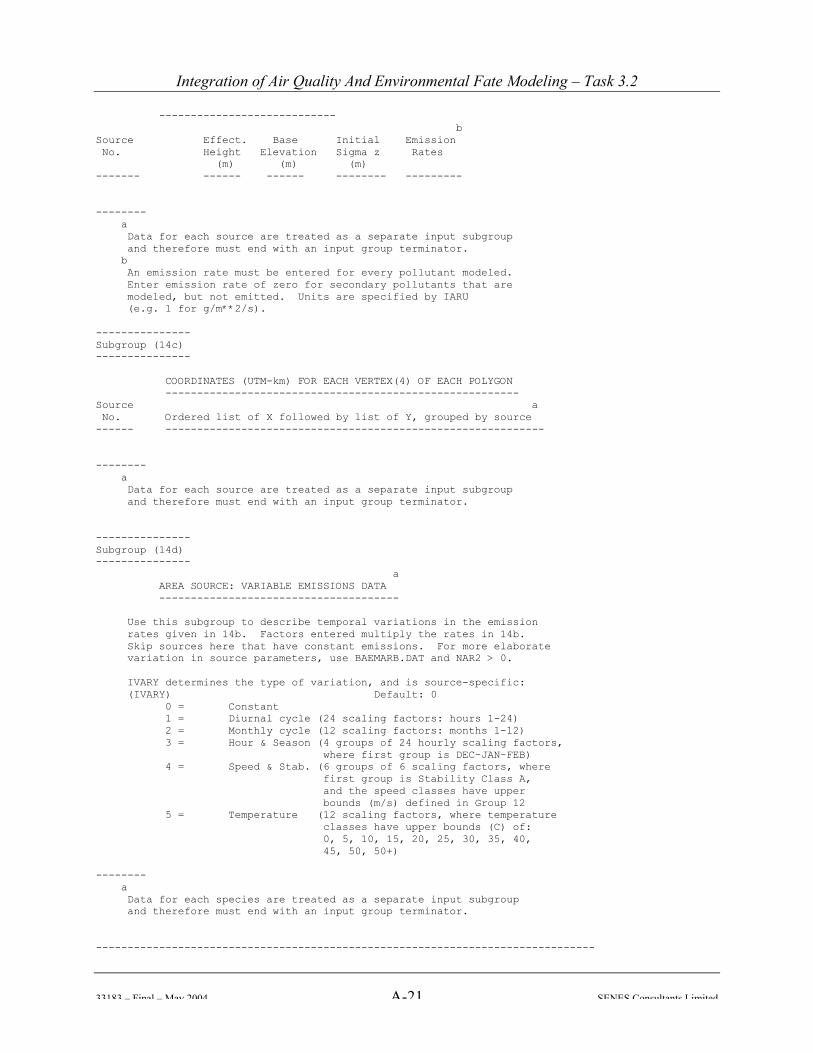
Integration of Air Quality And Environmental Fate Modeling – Task 3.2
33183 – Final – May 2004 A-21 SENES Consultants Limited
----------------------------
b
Source Effect. Base Initial Emission
No. Height Elevation Sigma z Rates
(m) (m) (m)
------- ------ ------ -------- ---------
--------
a
Data for each source are treated as a separate input subgroup
and therefore must end with an input group terminator.
b
An emission rate must be entered for every pollutant modeled.
Enter emission rate of zero for secondary pollutants that are
modeled, but not emitted. Units are specified by IARU
(e.g. 1 for g/m**2/s).
---------------
Subgroup (14c)
---------------
COORDINATES (UTM-km) FOR EACH VERTEX(4) OF EACH POLYGON
--------------------------------------------------------
Source a
No. Ordered list of X followed by list of Y, grouped by source
------ ------------------------------------------------------------
--------
a
Data for each source are treated as a separate input subgroup
and therefore must end with an input group terminator.
---------------
Subgroup (14d)
---------------
a
AREA SOURCE: VARIABLE EMISSIONS DATA
--------------------------------------
Use this subgroup to describe temporal variations in the emission
rates given in 14b. Factors entered multiply the rates in 14b.
Skip sources here that have constant emissions. For more elaborate
variation in source parameters, use BAEMARB.DAT and NAR2 > 0.
IVARY determines the type of variation, and is source-specific:
(IVARY) Default: 0
0 = Constant
1 = Diurnal cycle (24 scaling factors: hours 1-24)
2 = Monthly cycle (12 scaling factors: months 1-12)
3 = Hour & Season (4 groups of 24 hourly scaling factors,
where first group is DEC-JAN-FEB)
4 = Speed & Stab. (6 groups of 6 scaling factors, where
first group is Stability Class A,
and the speed classes have upper
bounds (m/s) defined in Group 12
5 = Temperature (12 scaling factors, where temperature
classes have upper bounds (C) of:
0, 5, 10, 15, 20, 25, 30, 35, 40,
45, 50, 50+)
--------
a
Data for each species are treated as a separate input subgroup
and therefore must end with an input group terminator.
-------------------------------------------------------------------------------

Integration of Air Quality And Environmental Fate Modeling – Task 3.2
33183 – Final – May 2004 A-22 SENES Consultants Limited
INPUT GROUPS: 15a, 15b, 15c -- Line source parameters
---------------------------
---------------
Subgroup (15a)
---------------
Number of buoyant line sources
with variable location and emission
parameters (NLN2) No default ! NLN2 = 0 !
(If NLN2 > 0, ALL parameter data for
these sources are read from the file: LNEMARB.DAT)
Number of buoyant line sources (NLINES) No default ! NLINES = 0 !
Units used for line source
emissions below (ILNU) Default: 1 ! ILNU = 1 !
1 = g/s
2 = kg/hr
3 = lb/hr
4 = tons/yr
5 = Odour Unit * m**3/s (vol. flux of odour compound)
6 = Odour Unit * m**3/min
7 = metric tons/yr
Number of source-species
combinations with variable
emissions scaling factors
provided below in (15c) (NSLN1) Default: 0 ! NSLN1 = 0 !
Maximum number of segments used to model
each line (MXNSEG) Default: 7 ! MXNSEG = 7 !
The following variables are required only if NLINES > 0. They are
used in the buoyant line source plume rise calculations.
Number of distances at which Default: 6 ! NLRISE = 6 !
transitional rise is computed
Average building length (XL) No default ! XL = .0 !
(in meters)
Average building height (HBL) No default ! HBL = .0 !
(in meters)
Average building width (WBL) No default ! WBL = .0 !
(in meters)
Average line source width (WML) No default ! WML = .0 !
(in meters)
Average separation between buildings (DXL) No default ! DXL = .0 !
(in meters)
Average buoyancy parameter (FPRIMEL) No default ! FPRIMEL = .0 !
(in m**4/s**3)
!END!
---------------
Subgroup (15b)
---------------
BUOYANT LINE SOURCE: CONSTANT DATA
----------------------------------
a
Source Beg. X Beg. Y End. X End. Y Release Base Emission
No. Coordinate Coordinate Coordinate Coordinate Height Elevation Rates

Integration of Air Quality And Environmental Fate Modeling – Task 3.2
33183 – Final – May 2004 A-23 SENES Consultants Limited
(km) (km) (km) (km) (m) (m)
------ ---------- ---------- --------- ---------- ------- --------- ---------
--------
a
Data for each source are treated as a separate input subgroup
and therefore must end with an input group terminator.
b
An emission rate must be entered for every pollutant modeled.
Enter emission rate of zero for secondary pollutants that are
modeled, but not emitted. Units are specified by ILNTU
(e.g. 1 for g/s).
---------------
Subgroup (15c)
---------------
a
BUOYANT LINE SOURCE: VARIABLE EMISSIONS DATA
----------------------------------------------
Use this subgroup to describe temporal variations in the emission
rates given in 15b. Factors entered multiply the rates in 15b.
Skip sources here that have constant emissions.
IVARY determines the type of variation, and is source-specific:
(IVARY) Default: 0
0 = Constant
1 = Diurnal cycle (24 scaling factors: hours 1-24)
2 = Monthly cycle (12 scaling factors: months 1-12)
3 = Hour & Season (4 groups of 24 hourly scaling factors,
where first group is DEC-JAN-FEB)
4 = Speed & Stab. (6 groups of 6 scaling factors, where
first group is Stability Class A,
and the speed classes have upper
bounds (m/s) defined in Group 12
5 = Temperature (12 scaling factors, where temperature
classes have upper bounds (C) of:
0, 5, 10, 15, 20, 25, 30, 35, 40,
45, 50, 50+)
--------
a
Data for each species are treated as a separate input subgroup
and therefore must end with an input group terminator.
-------------------------------------------------------------------------------
INPUT GROUPS: 16a, 16b, 16c -- Volume source parameters
---------------------------
---------------
Subgroup (16a)
---------------
Number of volume sources with
parameters provided in 16b,c (NVL1) No default ! NVL1 = 0 !
Units used for volume source
emissions below in 16b (IVLU) Default: 1 ! IVLU = 1 !
1 = g/s
2 = kg/hr
3 = lb/hr
4 = tons/yr
5 = Odour Unit * m**3/s (vol. flux of odour compound)

Integration of Air Quality And Environmental Fate Modeling – Task 3.2
33183 – Final – May 2004 A-24 SENES Consultants Limited
6 = Odour Unit * m**3/min
7 = metric tons/yr
Number of source-species
combinations with variable
emissions scaling factors
provided below in (16c) (NSVL1) Default: 0 ! NSVL1 = 0 !
Number of volume sources with
variable location and emission
parameters (NVL2) No default ! NVL2 = 0 !
(If NVL2 > 0, ALL parameter data for
these sources are read from the VOLEMARB.DAT file(s) )
!END!
---------------
Subgroup (16b)
---------------
a
VOLUME SOURCE: CONSTANT DATA
------------------------------
b
X UTM Y UTM Effect. Base Initial Initial Emission
Coordinate Coordinate Height Elevation Sigma y Sigma z Rates
(km) (km) (m) (m) (m) (m)
---------- ---------- ------ ------ -------- -------- --------
--------
a
Data for each source are treated as a separate input subgroup
and therefore must end with an input group terminator.
b
An emission rate must be entered for every pollutant modeled.
Enter emission rate of zero for secondary pollutants that are
modeled, but not emitted. Units are specified by IVLU
(e.g. 1 for g/s).
---------------
Subgroup (16c)
---------------
a
VOLUME SOURCE: VARIABLE EMISSIONS DATA
----------------------------------------
Use this subgroup to describe temporal variations in the emission
rates given in 16b. Factors entered multiply the rates in 16b.
Skip sources here that have constant emissions. For more elaborate
variation in source parameters, use VOLEMARB.DAT and NVL2 > 0.
IVARY determines the type of variation, and is source-specific:
(IVARY) Default: 0
0 = Constant
1 = Diurnal cycle (24 scaling factors: hours 1-24)
2 = Monthly cycle (12 scaling factors: months 1-12)
3 = Hour & Season (4 groups of 24 hourly scaling factors,
where first group is DEC-JAN-FEB)
4 = Speed & Stab. (6 groups of 6 scaling factors, where
first group is Stability Class A,
and the speed classes have upper
bounds (m/s) defined in Group 12
5 = Temperature (12 scaling factors, where temperature
classes have upper bounds (C) of:
0, 5, 10, 15, 20, 25, 30, 35, 40,
45, 50, 50+)

Integration of Air Quality And Environmental Fate Modeling – Task 3.2
33183 – Final – May 2004 A-25 SENES Consultants Limited
--------
a
Data for each species are treated as a separate input subgroup
and therefore must end with an input group terminator.
-------------------------------------------------------------------------------
INPUT GROUPS: 17a & 17b -- Non-gridded (discrete) receptor information
-----------------------
---------------
Subgroup (17a)
---------------
Number of non-gridded receptors (NREC) No default ! NREC = 0 !
!END!
---------------
Subgroup (17b)
---------------
a
NON-GRIDDED (DISCRETE) RECEPTOR DATA
------------------------------------
X UTM Y UTM Ground Height b
Receptor Coordinate Coordinate Elevation Above Ground
No. (km) (km) (m) (m)
-------- ---------- ---------- --------- ------------
-------------
a
Data for each receptor are treated as a separate input subgroup
and therefore must end with an input group terminator.
b
Receptor height above ground is optional. If no value is entered,
the receptor is placed on the ground.