Boundary-Layer Meteorol (2011) 140:471–489DOI 10.1007/s10546-011-9620-6

ARTICLE

Combining a Detailed Building Energy Modelwith a Physically-Based Urban Canopy Model

Bruno Bueno · Leslie Norford · Grégoire Pigeon ·Rex Britter

Received: 26 March 2010 / Accepted: 26 April 2011 / Published online: 25 May 2011© Springer Science+Business Media B.V. 2011

Abstract A scheme that couples a detailed building energy model, EnergyPlus, and anurban canopy model, the Town Energy Balance (TEB), is presented. Both models arewell accepted and evaluated within their individual scientific communities. The coupledscheme proposes a more realistic representation of buildings and heating, ventilation andair-conditioning (HVAC) systems, which allows a broader analysis of the two-way inter-actions between the energy performance of buildings and the urban climate around thebuildings. The scheme can be used to evaluate the building energy models that are beingdeveloped within the urban climate community. In this study, the coupled scheme is eval-uated using measurements conducted over the dense urban centre of Toulouse, France.The comparison includes electricity and natural gas energy consumption of buildings,building façade temperatures, and urban canyon air temperatures. The coupled scheme isthen used to analyze the effect of different building and HVAC system configurations onbuilding energy consumption, waste heat released from HVAC systems, and outdoor airtemperatures for the case study of Toulouse. Three different energy efficiency strategies areanalyzed: shading devices, economizers, and heat recovery.

Keywords Anthropogenic heat · Building simulation model ·Heating ventilation air-conditioning · Town energy balance · Urban heat island

1 Introduction

In the context of analyzing and mitigating the increase in air temperature produced by urban-ization and known as the urban heat island (UHI) effect, heat release from buildings at nightand anthropogenic sources play a critical role (Sailor 2010). To account for building effects,

B. Bueno (B) · L. Norford · R. BritterMassachusetts Institute of Technology, 77 Massachusetts Ave., R.5-414, Cambridge, 02139 MA, USAe-mail: bbueno@mit.edu

G. PigeonCNRM-GAME, Météo France and CNRS, Toulouse, France

123

472 B. Bueno et al.

urban climatologists have developed simplified building energy models integrated into urbancanopy models (Kikegawa et al. 2003; Salamanca et al. 2010). The ability of these modelsto analyze the interactions between buildings and the urban environment has been verified(Kondo and Kikegawa 2003; Salamanca and Martilli 2010), including the effect of the wasteheat released from heating, ventilation and air-conditioning (HVAC) systems (Kikegawa et al.2006; Ihara et al. 2008).

While these building parametrizations represent a significant advancement in integratingbuilding energy and urban climate studies, they still have limitations that affect the evalua-tion of building energy consumption and the calculation of waste heat released from HVACsystems. In particular, they use an idealized representation of HVAC systems that neglectsthe specificities of the different HVAC configurations and that does not allow the assessmentof energy efficiency strategies. In addition, they usually do not implement models of passivebuilding systems such as shading devices or natural ventilation and they do not performdaylighting analyses.

This article presents a method to integrate building energy and urban climate studies, bycoupling a detailed building energy model, EnergyPlus (Crawley et al. 2001), and an urbancanopy model, the Town Energy Balance (TEB) (Masson 2000). The Energy Plus-TEBcoupled scheme intentionally combines models that have already been extensively used andevaluated and are well known and accepted within their respective communities, buildingengineering and urban climatology.

The coupled scheme makes it possible to analyze the effect on urban climate of allbuilding and building system parameters included in a detailed building model. It also enablesthe identification of building and building system configurations whose analysis and designare more sensitive to urban climate conditions. Furthermore, it can be used in the evaluationprocess of simplified building models integrated into urban canopy models. As a backdrop tothis article, the authors recognize the opportunities arising at the intersection of the buildingengineering and the urban climatology communities in the context of climate modification,increasing urbanization, and future energy scarcity.

We first present an overview of building energy modelling as related to urban climatestudies. Next, the coupled scheme is described and evaluated against field data from theexperiment CAPITOUL conducted in Toulouse, France (Masson et al. 2008). The coupledscheme is then used to study the impact of different building and HVAC system configura-tions on the energy consumption of buildings, HVAC waste heat emissions, and outdoor airtemperatures. Conclusions and applications are presented in Sect. 6.

2 Urban Climate and Building Energy Modelling

2.1 The Town Energy Balance (TEB) Model

The TEB model (Masson 2000) is a physically based urban canopy model that represents thefluid dynamic and thermodynamic effects of an urbanized area on the atmosphere. The TEBmodel has been evaluated with observations in various urban sites and weather conditions(Masson et al. 2002; Lemonsu et al. 2004; Offerle et al. 2005; Pigeon et al. 2008). The modelconsiders a two-dimensional approximation of an urban canyon formed by three genericsurfaces: a wall, a road, and a roof, and calculates the climate conditions, the drag forceand energy fluxes of a town or neighbourhood formed by identical urban canyons, where allorientations are possible and all exist with the same probability.

123

Combining a Detailed Building Energy Model 473

The TEB model implements a simple representation of building energy processes by solv-ing a transient heat conduction equation through a multi-layered wall and roof. The force-restore method is applied to calculate indoor conditions from the contributions of the differentbuilding surfaces. Further developments of the TEB model include a minimum threshold tocalculate the heating loads of the building associated with transmission through building sur-faces (Pigeon et al. 2008). Other phenomena, such as transmission through windows, internalheat gains, infiltration and the calculation of cooling loads, are not yet included.

2.2 Building Parametrizations

A further step in representing the effects of buildings on urban climate was carried out byKikegawa et al. (2003), who implemented a simplified building energy model in an urbancanopy parametrization for mesoscale models. In addition to solving the diffusion equationfor walls, this model takes into account the internal sources of heat, solar radiation transmit-ted through windows, and the energy loads due to ventilation. Applying sensible and latentheat balances, the model calculates the energy demand required to maintain certain indoorconditions.

Recently, Salamanca et al. (2010) developed a new building energy model, coupled witha multi-layer urban canopy model (Martilli et al. 2002). This model allows the definition ofmultiple-story buildings and incorporates a more detailed treatment of windows, includingthe calculation of the transmitted solar radiation as a function of the angle of incidence.A range of comfort conditions and a maximum capacity of the HVAC system can also bespecified in this model.

The building energy models of Kikegawa and Salamanca are able to capture the main heattransfer processes that occur inside buildings (Salamanca et al. 2010). They are also ableto predict the energy demand of a basic building configuration and to estimate the energyconsumption and waste heat emissions of an HVAC system (Ihara et al. 2008; Salamancaand Martilli 2010). Generally, these building parametrizations have been developed withinthe urban climatology community.

2.3 EnergyPlus

One industry-standard building energy model, EnergyPlus (Crawley et al. 2001), developedby the building engineering community, calculates the energy demand of a building byapplying a heat balance method (DOE 2010a), somewhat similar to that used in the above-mentioned building parametrizations. It also implements detailed models for external heattransfer calculations such as convection, solar radiation (including shadows and reflections),and longwave radiation exchange with the sky (DOE 2010a). EnergyPlus has been extensivelyevaluated according to building simulation standards (e.g. DOE 2010b,c).

One difference with respect to building parametrizations is that EnergyPlus can calcu-late the energy consumption of a specific HVAC system by solving the sensible and latentenergy transformations of a working fluid (air or water) when this passes through the dif-ferent HVAC components (coils, fans, heating and cooling plant equipment, economizers,cooling towers, etc.). Examples of specific HVAC systems are variable-air-volume, fan-coils,or chilled ceilings with dedicated outdoor air systems.

This detailed definition is intended to capture the real performance of HVAC systems thatsupply energy to cover the energy demand of the building and to counteract thermal lossesthrough the system. The capacity of the system depends on the conditions inside and outside

123

474 B. Bueno et al.

the building, and there are situations where the system is not able to supply the requiredenergy, affecting the resulting indoor conditions. Cooling-system efficiency (as measured bythe coefficient of performance (COP), the dimensionless ratio of thermal output to fuel input)also depends on the conditions inside and outside the building and on the part load ratio ofthe cooling plant. The latter takes into account the loss of efficiency when the cooling plantis not working at its maximum capacity.

In an ideal building energy model, the indoor air humidity is assumed constant and thelatent energy supplied or removed by the HVAC system is directly equal to the latent energydemand of the building. On the contrary, a detailed definition solves for the dehumidificationof the air passing through a cooling system. In many HVAC system configurations, the indoorair humidity is not controlled in the same way as the air temperature, so the calculation ofthe air humidity requires a psychrometric model of the air crossing the system. This capa-bility allows a more realistic analysis of the latent heat exchange between the indoor and theoutdoor environments.

Another difference between detailed building energy models and building parametriza-tions is the capability of modelling building demand reduction strategies or passive sys-tems. Passive systems take advantage of the sun, the wind and environmental conditionsto reduce or eliminate the need for HVAC systems. Accurate simulation of their effect issometimes crucial in predicting the overall energy performance of buildings and conse-quently the heat released from buildings into the environment. Examples of passive systemsare shading devices, double-skin façades, natural ventilation, heat storage devices, evapo-rative cooling, earth tubes for pre-heating or pre-cooling ventilation air, and cool or greenroofs.

Finally, detailed building energy models can make daylighting calculations and includethem in the thermal energy balance of buildings. Lights can contribute significantly tobuilding energy end-use, both directly (11.3% according to DOE 2009) and by adding heatingloads, which affect the eventual waste heat released from HVAC systems.

3 The Coupled Scheme

The coupled scheme combines EnergyPlus and the TEB model to calculate the energy per-formance of buildings and the urban climate around the buildings, taking into account thereciprocal interactions between the two.

3.1 Definition of a Reference Building in EnergyPlus

The current version of the coupled scheme is able to analyze an average-oriented urban can-yon (Masson 2000). A box-type reference building is defined in EnergyPlus assuming anurban area composed of a regular grid of square-plan buildings (Fig. 1). The geometry ofthe reference building is obtained using TEB urban morphology parameters: building height(hbld), building horizontal area density (ρbld), and vertical to horizontal urban surface ratio(VH), viz.

ρbld = a2/ (a/2 + b/2)2 , (1)

V H = 4ahbld/ (a/2 + b/2)2 . (2)

In these expressions, a is the side of the square-plan building and b is the side of the squareformed by the projection of the surrounding buildings façades on the ground (Fig. 2). Thegeometric unit of the urban grid used to derive Eqs. 1 and 2 is indicated with a broken-dash

123

Combining a Detailed Building Energy Model 475

Fig. 1 Plan view of an urbanarea composed of a homogeneousgrid of square-plan buildings.The geometric unit of the grid isindicated with a broken-dash line

Fig. 2 Plan view of the reference building defined in the EnergyPlus model, indicating building walls, build-ing windows and surrounding buildings. The building is rotated 45◦ with respect to the north–south axis.The geometric unit of the grid is indicated with a broken-dash line. The dimension parameters a and b arecalculated from the TEB model’s morphology parameters

line in both Figs. 1 and 2. The reference building is composed of a single zone with an inter-nal thermal mass representing intermediate floor constructions. Windows are defined suchthat their vertical dimension matches the vertical dimension of building façades, and theirhorizontal dimension is a fraction of the horizontal dimension of building façades accordingto the glazing ratio. Surrounding buildings are represented by shadowing surfaces. The solarradiation received by the four vertical surfaces of the reference building approaches the solarradiation received by walls in the average-oriented canyon calculated by the TEB model. Acloser agreement to the average-oriented canyon approach can be achieved by rotating thebuilding 45◦ with respect to the north–south axis (Fig. 2).

3.2 Exchanged Information

Both EnergyPlus and the TEB model are able to calculate exterior wall and roof surfacetemperatures. In the coupled scheme, these surface temperatures are calculated by TEB andthen used in EnergyPlus as boundary conditions. One of the reasons for this choice is thatEnergyPlus simplifies the calculation of longwave radiation between a building surface and

123

476 B. Bueno et al.

the surrounding urban surfaces, assuming that the latter are at the outdoor air tempera-ture. Wall convective heat transfer correlations (CHTC) also differ between the two models.Palyvos (2008) presented a literature review of CHTC applied to building surfaces, and pro-posed a generic correlation more similar to the one used in TEB (Masson 2000) than to thatused in EnergyPlus (DOE 2010a).

The original version of the TEB model is only able to calculate surface temperatures asso-ciated with the fraction of façades covered by walls, neglecting the effect of windows in theoutdoor energy balance. Window surface temperatures can be significantly different fromwall surface temperatures and are more affected by the indoor environment. The coupledscheme uses an adapted version of TEB that is able to use the window temperatures calcu-lated by EnergyPlus in its outdoor energy balance according to the glazing ratio of buildingfaçades. Solar reflections, convective and radiative heat exchanges are modified in TEBaccordingly.

EnergyPlus also calculates the waste heat released from HVAC systems. In compressionrefrigeration cycles (the most common cooling systems), waste heat emissions (Qwaste) canbe calculated by adding the heat exchanged between the HVAC system and the building(Qexch) and the energy consumption of the HVAC system (Qcons), Qwaste = Qexch + Qcons.In fuel-combustion heating systems, waste heat emissions correspond to the combustiongases exhausted from chimneys and are calculated as Qwaste = Qcons − Qexch. The energyexchanged between the HVAC system and the building, and the energy consumed by thesystem, are calculated by EnergyPlus taking into account the interactions among system,building, and environment. The resulting waste heat emissions are included in the outdoorenergy balance of TEB as a wall-distributed energy source.

3.3 Iterative Coupling Method

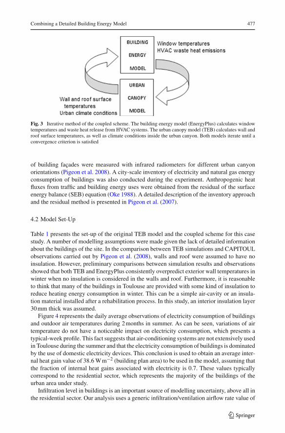
The coupled scheme uses an iterative method to calculate the interactions between Ener-gyPlus and the TEB model. The iterative coupling process starts from a preliminary TEBsimulation using off-line meteorological forcing information (for details, see Masson et al.2002). The wall temperatures, roof temperatures, and urban canyon climate conditions cal-culated by TEB are supplied as boundary conditions to an EnergyPlus simulation. Then,window temperatures and HVAC waste heat emissions calculated by EnergyPlus are used ina new iteration of TEB. This process (Fig. 3) is repeated until a convergence criterion is satis-fied. In the present study, convergence was assumed to be reached when the average canyontemperature difference between iterations fell below 0.05◦C. This was typically achievedafter two or three iterations.

4 Comparison with Field Data

4.1 Observations

This section presents a comparison between the coupled scheme, the original TEB model,and the measurements obtained during the experiment CAPITOUL carried out in Toulouse(France) from February 2004 to March 2005 (Masson et al. 2008). During the experiment,forcing measurements were taken in the dense urban centre of Toulouse at 27.5 m above theaverage building height and 47.5 m above the ground. In the same area, urban air tempera-tures were obtained from a sensor installed at the top of a street canyon. Surface temperatures

123

Combining a Detailed Building Energy Model 477

Fig. 3 Iterative method of the coupled scheme. The building energy model (EnergyPlus) calculates windowtemperatures and waste heat release from HVAC systems. The urban canopy model (TEB) calculates wall androof surface temperatures, as well as climate conditions inside the urban canyon. Both models iterate until aconvergence criterion is satisfied

of building façades were measured with infrared radiometers for different urban canyonorientations (Pigeon et al. 2008). A city-scale inventory of electricity and natural gas energyconsumption of buildings was also conducted during the experiment. Anthropogenic heatfluxes from traffic and building energy uses were obtained from the residual of the surfaceenergy balance (SEB) equation (Oke 1988). A detailed description of the inventory approachand the residual method is presented in Pigeon et al. (2007).

4.2 Model Set-Up

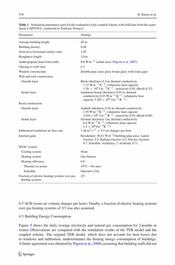
Table 1 presents the set-up of the original TEB model and the coupled scheme for this casestudy. A number of modelling assumptions were made given the lack of detailed informationabout the buildings of the site. In the comparison between TEB simulations and CAPITOULobservations carried out by Pigeon et al. (2008), walls and roof were assumed to have noinsulation. However, preliminary comparisons between simulation results and observationsshowed that both TEB and EnergyPlus consistently overpredict exterior wall temperatures inwinter when no insulation is considered in the walls and roof. Furthermore, it is reasonableto think that many of the buildings in Toulouse are provided with some kind of insulation toreduce heating energy consumption in winter. This can be a simple air-cavity or an insula-tion material installed after a rehabilitation process. In this study, an interior insulation layer30 mm thick was assumed.

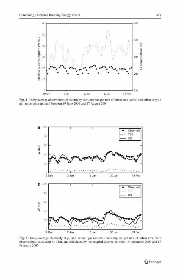
Figure 4 represents the daily average observations of electricity consumption of buildingsand outdoor air temperatures during 2 months in summer. As can be seen, variations of airtemperature do not have a noticeable impact on electricity consumption, which presents atypical-week profile. This fact suggests that air-conditioning systems are not extensively usedin Toulouse during the summer and that the electricity consumption of buildings is dominatedby the use of domestic electricity devices. This conclusion is used to obtain an average inter-nal heat gain value of 38.6 W m−2 (building plan area) to be used in the model, assuming thatthe fraction of internal heat gains associated with electricity is 0.7. These values typicallycorrespond to the residential sector, which represents the majority of the buildings of theurban area under study.

Infiltration level in buildings is an important source of modelling uncertainty, above all inthe residential sector. Our analysis uses a generic infiltration/ventilation airflow rate value of

123

478 B. Bueno et al.

Table 1 Simulation parameters used for the evaluation of the coupled scheme with field data from the exper-iment CAPITOUL conducted in Toulouse (France)

Parameters Settings

Average building height 20 m

Building density 0.68

Vertical to horizontal surface ratio 1.05

Roughness length 2.0 m

Anthropogenic heat from traffic 8.0 W m−2 (urban area) (Pigeon et al. 2007)

Glazing-to-wall ratio 0.3

Window construction Double pane clear glass (6 mm glass with 6 mm gap)

Wall and roof construction

Outside layer Brick (thickness 0.3 m; thermal conductivity1.15 W m−1 K−1; volumetric heat capacity1.58 × 106 J m−3 K−1 ; emissivity 0.95; albedo 0.32)

Inside layer Insulation board (thickness 0.03 m; thermalconductivity 0.03 W m−1 K−1; volumetric heatcapacity 5.203 × 104 J m−3 K−1)

Road construction

Outside layer Asphalt (thickness 0.24 m; thermal conductivity1.95 W m−1K−1; volumetric heat capacity2.016 ×106 J m−3 K−1 ; emissivity 0.94; albedo 0.08)

Inside layer Ground (thickness 1 m; thermal conductivity0.4 W m−1 K−1; volumetric heat capacity1.4 × 106J m−3K−1)

Infiltration/ventilation air flow rate 7.46 m3 s−1 = 0.5 air changes per hour

Internal gains Residential: 38.61 W m−2(building plan area). Latentfraction: 0.2; Radiant fraction: 0.2; Electric fraction:0.7. Schedule: weekdays, 1; weekend, 0.71.

HVAC system

Cooling system None

Heating system Gas furnace

Heating efficiency 0.9

Thermal set points 19◦C—No max.

Schedule Operative 24 h

Fraction of electric heating systems over gasheating systems

2/3

0.5 ACH (room air volume changes per hour). Finally, a fraction of electric heating systemsover gas heating systems of 2/3 was also assumed.

4.3 Building Energy Consumption

Figure 5 shows the daily average electricity and natural gas consumption for 2 months inwinter. Observations are compared with the simulation results of the TEB model and thecoupled scheme. The original TEB model, which does not account for heat losses dueto windows and infiltration, underestimates the heating energy consumption of buildings.A better agreement was obtained by Pigeon et al. (2008) assuming that building walls did not

123

Combining a Detailed Building Energy Model 479

Fig. 4 Daily average observations of electricity consumption per unit of urban area (solid) and urban canyonair temperature (points) between 19 June 2004 and 17 August 2004

a

b

Fig. 5 Daily average electricity (top) and natural gas (bottom) consumption per unit of urban area fromobservations, calculated by TEB, and calculated by the coupled scheme between 19 December 2004 and 17February 2005

123

480 B. Bueno et al.

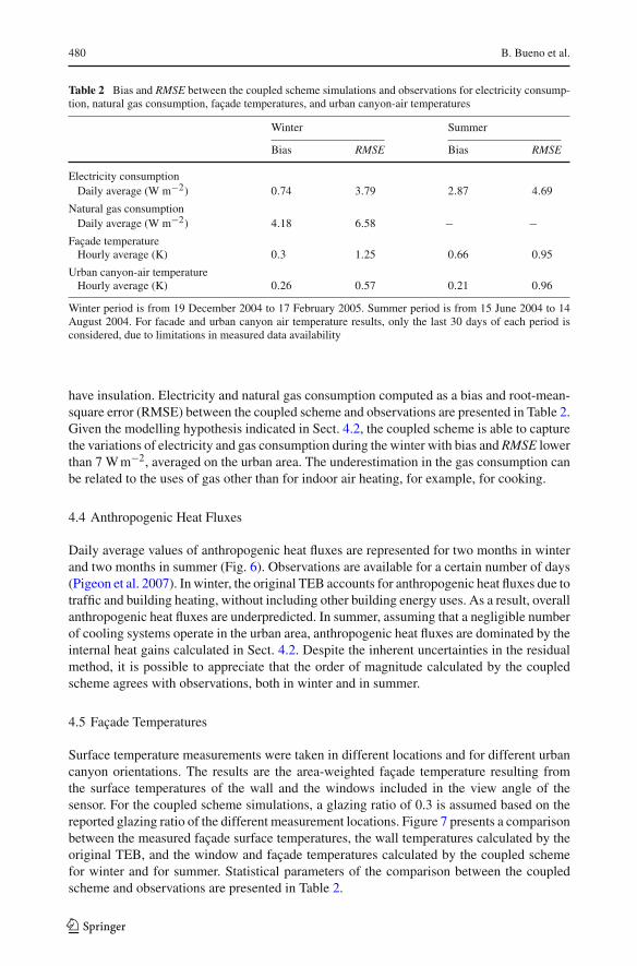
Table 2 Bias and RMSE between the coupled scheme simulations and observations for electricity consump-tion, natural gas consumption, façade temperatures, and urban canyon-air temperatures

Winter Summer

Bias RMSE Bias RMSE

Electricity consumptionDaily average (W m−2) 0.74 3.79 2.87 4.69

Natural gas consumptionDaily average (W m−2) 4.18 6.58 − −

Façade temperatureHourly average (K) 0.3 1.25 0.66 0.95

Urban canyon-air temperatureHourly average (K) 0.26 0.57 0.21 0.96

Winter period is from 19 December 2004 to 17 February 2005. Summer period is from 15 June 2004 to 14August 2004. For facade and urban canyon air temperature results, only the last 30 days of each period isconsidered, due to limitations in measured data availability

have insulation. Electricity and natural gas consumption computed as a bias and root-mean-square error (RMSE) between the coupled scheme and observations are presented in Table 2.Given the modelling hypothesis indicated in Sect. 4.2, the coupled scheme is able to capturethe variations of electricity and gas consumption during the winter with bias and RMSE lowerthan 7 W m−2, averaged on the urban area. The underestimation in the gas consumption canbe related to the uses of gas other than for indoor air heating, for example, for cooking.

4.4 Anthropogenic Heat Fluxes

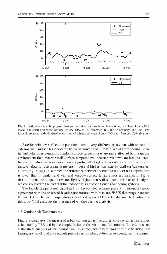
Daily average values of anthropogenic heat fluxes are represented for two months in winterand two months in summer (Fig. 6). Observations are available for a certain number of days(Pigeon et al. 2007). In winter, the original TEB accounts for anthropogenic heat fluxes due totraffic and building heating, without including other building energy uses. As a result, overallanthropogenic heat fluxes are underpredicted. In summer, assuming that a negligible numberof cooling systems operate in the urban area, anthropogenic heat fluxes are dominated by theinternal heat gains calculated in Sect. 4.2. Despite the inherent uncertainties in the residualmethod, it is possible to appreciate that the order of magnitude calculated by the coupledscheme agrees with observations, both in winter and in summer.

4.5 Façade Temperatures

Surface temperature measurements were taken in different locations and for different urbancanyon orientations. The results are the area-weighted façade temperature resulting fromthe surface temperatures of the wall and the windows included in the view angle of thesensor. For the coupled scheme simulations, a glazing ratio of 0.3 is assumed based on thereported glazing ratio of the different measurement locations. Figure 7 presents a comparisonbetween the measured façade surface temperatures, the wall temperatures calculated by theoriginal TEB, and the window and façade temperatures calculated by the coupled schemefor winter and for summer. Statistical parameters of the comparison between the coupledscheme and observations are presented in Table 2.

123

Combining a Detailed Building Energy Model 481

a

b

Fig. 6 Daily average anthropogenic heat per unit of urban area from observations, calculated by the TEBmodel, and calculated by the coupled scheme between 19 December 2004 and 17 February 2005 (top); andfrom observations and calculated by the coupled scheme between 19 June 2004 and 17 August 2004 (bottom)

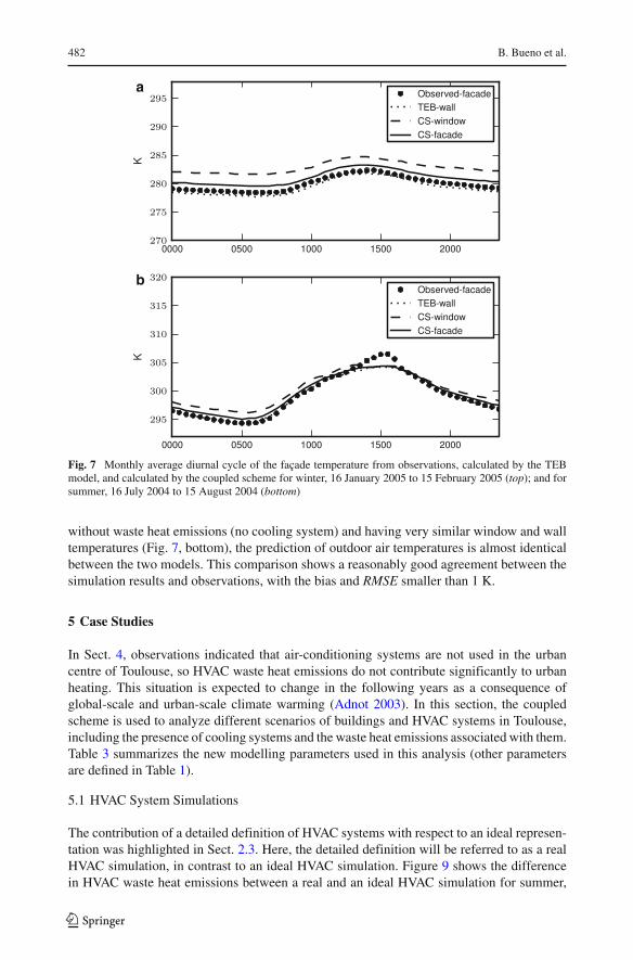
Exterior window surface temperatures have a very different behaviour with respect toexterior wall surface temperatures between winter and summer. Apart from thermal iner-tia and solar considerations, window surface temperatures are more affected by the indoorenvironment than exterior wall surface temperatures, because windows are less insulated.In winter, indoor air temperatures are significantly higher than outdoor air temperatures;thus, window surface temperatures are in general higher than exterior wall surface temper-atures (Fig. 7, top). In summer, the difference between indoor and outdoor air temperaturesis lower than in winter, and wall and window surface temperatures are similar. In Fig. 7(bottom), window temperatures are slightly higher than wall temperatures during the night,which is related to the fact that the indoor air is not conditioned (no cooling system).

The façade temperatures calculated by the coupled scheme present a reasonably goodagreement with the observed façade temperatures with bias and RMSE that range between0.3 and 1.3 K. The wall temperatures calculated by the TEB model also match the observa-tions, but TEB excludes the presence of windows in the analysis.

4.6 Outdoor Air Temperatures

Figure 8 compares the measured urban canyon air temperatures with the air temperaturescalculated by TEB and by the coupled scheme for winter and for summer. Table 2 presentsa statistical analysis of this comparison. In winter, waste heat emissions due to indoor airheating are small, and both models predict very similar outdoor air temperatures. In summer,

123

482 B. Bueno et al.

a

b

Fig. 7 Monthly average diurnal cycle of the façade temperature from observations, calculated by the TEBmodel, and calculated by the coupled scheme for winter, 16 January 2005 to 15 February 2005 (top); and forsummer, 16 July 2004 to 15 August 2004 (bottom)

without waste heat emissions (no cooling system) and having very similar window and walltemperatures (Fig. 7, bottom), the prediction of outdoor air temperatures is almost identicalbetween the two models. This comparison shows a reasonably good agreement between thesimulation results and observations, with the bias and RMSE smaller than 1 K.

5 Case Studies

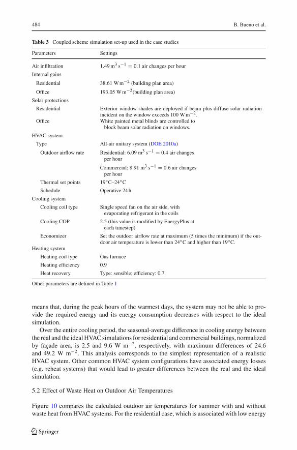
In Sect. 4, observations indicated that air-conditioning systems are not used in the urbancentre of Toulouse, so HVAC waste heat emissions do not contribute significantly to urbanheating. This situation is expected to change in the following years as a consequence ofglobal-scale and urban-scale climate warming (Adnot 2003). In this section, the coupledscheme is used to analyze different scenarios of buildings and HVAC systems in Toulouse,including the presence of cooling systems and the waste heat emissions associated with them.Table 3 summarizes the new modelling parameters used in this analysis (other parametersare defined in Table 1).

5.1 HVAC System Simulations

The contribution of a detailed definition of HVAC systems with respect to an ideal represen-tation was highlighted in Sect. 2.3. Here, the detailed definition will be referred to as a realHVAC simulation, in contrast to an ideal HVAC simulation. Figure 9 shows the differencein HVAC waste heat emissions between a real and an ideal HVAC simulation for summer,

123

Combining a Detailed Building Energy Model 483

a

b

Fig. 8 Monthly average diurnal cycle of the urban canyon air temperature from observations, calculated bythe TEB model, and calculated by the coupled scheme for winter, 16 January 2005 to 15 February 2005 (top);and for summer, 16 July 2004 to 15 August 2004 (bottom)

which ranges between 7 and 13%. Two different building uses are represented: residentialand commercial (Table 3). Different levels of waste heat emissions are predicted for theresidential and the commercial buildings, around 60 and 190 W m−2, respectively, averagedon the urban area. A similar study carried out by Salamanca and Martilli (2010) predictedwaste heat emissions in Basel (Switzerland) at summertime that ranged between 90 and160 W m−2.

The differences between the real and the ideal HVAC simulations are mainly related tothe calculated latent heat exchanged between the HVAC system and the building. In the idealsimulation, the exchanged latent heat is directly equal to the latent energy demand of thebuilding. In the real case, and in a typical situation where the system is only controlled bya thermostat (no humidity control), the exchanged latent heat is a consequence of the dehu-midification of the air passing through the system, when this is cooled to meet the sensibleenergy demand of the building.

The fact that the evolution of waste heat during the day is less dynamic in the real casethan in the ideal case can be explained by two effects that are captured by the real simulationand not by the ideal simulation. First, when the system is working at night, it experiencesa loss of efficiency due to working at part load. It also experiences a gain of efficiencydue to lower condenser temperatures; but, in this case, the first effect dominates. As aresult, the energy consumption from the real simulation is higher than the one obtainedfrom the ideal simulation. Second, the real HVAC system has a limited capacity, which

123

484 B. Bueno et al.

Table 3 Coupled scheme simulation set-up used in the case studies

Parameters Settings

Air infiltration 1.49 m3 s−1 = 0.1 air changes per hour

Internal gains

Residential 38.61 W m−2 (building plan area)

Office 193.05 W m−2(building plan area)

Solar protections

Residential Exterior window shades are deployed if beam plus diffuse solar radiationincident on the window exceeds 100 W m−2.

Office White painted metal blinds are controlled toblock beam solar radiation on windows.

HVAC system

Type All-air unitary system (DOE 2010a)

Outdoor airflow rate Residential: 6.09 m3 s−1 = 0.4 air changesper hour

Commercial: 8.91 m3 s−1 = 0.6 air changesper hour

Thermal set points 19◦C–24◦C

Schedule Operative 24 h

Cooling system

Cooling coil type Single speed fan on the air side, withevaporating refrigerant in the coils

Cooling COP 2.5 (this value is modified by EnergyPlus ateach timestep)

Economizer Set the outdoor airflow rate at maximum (5 times the minimum) if the out-door air temperature is lower than 24◦C and higher than 19◦C.

Heating system

Heating coil type Gas furnace

Heating efficiency 0.9

Heat recovery Type: sensible; efficiency: 0.7.

Other parameters are defined in Table 1

means that, during the peak hours of the warmest days, the system may not be able to pro-vide the required energy and its energy consumption decreases with respect to the idealsimulation.

Over the entire cooling period, the seasonal-average difference in cooling energy betweenthe real and the ideal HVAC simulations for residential and commercial buildings, normalizedby façade area, is 2.5 and 9.6 W m−2, respectively, with maximum differences of 24.6and 49.2 W m−2. This analysis corresponds to the simplest representation of a realisticHVAC system. Other common HVAC system configurations have associated energy losses(e.g. reheat systems) that would lead to greater differences between the real and the idealsimulation.

5.2 Effect of Waste Heat on Outdoor Air Temperatures

Figure 10 compares the calculated outdoor air temperatures for summer with and withoutwaste heat from HVAC systems. For the residential case, which is associated with low energy

123

Combining a Detailed Building Energy Model 485

a

b

Fig. 9 Monthly average diurnal cycle of HVAC waste heat emissions per unit of façade area from a real andan ideal HVAC simulation of a residential (top) and a commercial building (bottom) for summer, 16 July 2004to 15 August 2004

Fig. 10 Monthly average diurnal cycle of the urban canyon air temperature from a coupled scheme simulationof a residential and a commercial building for summer, 16 July 2004 to 15 August 2004

consumption and waste heat emissions, the average increase in outdoor air temperature is0.8 K. In the commercial case, the average increase in the outdoor air temperature is 2.8 K.Similar values of air temperature increase due to HVAC systems have been reported previ-ously (Kikegawa et al. 2003; Ohashi et al. 2007; Hamilton et al. 2009).

123

486 B. Bueno et al.

Table 4 Annual energy savings and average waste heat reduction associated with the use of shading devices,economizers, and heat recovery systems

Annual energy savings perunit of building plan area

Average waste heat reductionper unit of façade area

Absolute(kWh m−2)

Relative (%) Absolute(W m−2)

Relative (%)

Shading devices (Cooling)Residential 24.0 20.50 8.5 28.83

Commercial 26.5 5.60 10.2 5.06

Economizers (Cooling)Residential 8.7 7.44 3.3 14.80

Commercial 27.1 3.60 4.3 3.21

Heat recovery (Heating)Residential 153.8 49.57 3.1 60.02

Energy savings and waste heat reductions are referred to the cooling system for shading devices and econo-mizers and to the heating system for the heat recovery

5.3 Effect of Shading Devices on Energy Consumption and HVAC Waste Heat Emissions

Shading devices are passive systems that reduce the transmitted solar radiation into thebuilding. Ideally, these devices should block direct solar radiation in the cooling period(summer), but allow the transmission of diffuse solar radiation for daylight purposes. Theyshould also allow solar heat transmission in the heating period (winter) provided that there areno glare issues. In this analysis, two different shading devices typically used for residentialand for commercial buildings in Toulouse are considered (Table 3).

Table 4 presents the annual cooling energy savings and average waste heat reductionassociated with the use of shading devices in summer for residential and commercial build-ings. Residential buildings, whose cooling loads are more sensitive to the transmitted solarradiation due to the low internal heat gains, can achieve reductions in energy savings andwaste heat emissions of 21 and 29%, respectively, by using shading devices. Having a similarabsolute value of waste heat reduction (similar impact on the outdoor environment), commer-cial buildings present lower relative values of energy consumption and waste heat reductionthan residential buildings (around 5%).

5.4 Effect of Economizers on Energy Consumption and HVAC Waste Heat Emissions

An economizer allows more than the minimum outdoor airflow to enter the building whenthe outdoor temperature is favourable (cooler than indoors in summer). This reduces theconsumption of the cooling plant and its waste heat emissions but penalizes the electricityconsumption of fans. The application of economizers can be useful in commercial build-ings when outdoor air temperatures are below the cooling set point and buildings still havecooling energy demand due to internal heat gains. In residential buildings, the same effectis usually achieved by means of natural ventilation (opening the windows), which does notrequire the electricity consumption of a fan. The effectiveness of these strategies is verysensitive to increases in outdoor air temperatures, which reduce the amount of time theycan operate. For the purposes of this analysis, an economizer is also applied to the residen-tial case instead of a natural ventilation system. The main difference is the outdoor airflow

123

Combining a Detailed Building Energy Model 487

passing through the building, which is constant for an economizer and variable for a naturalventilation system. The results of this analysis provide an upper limit for natural ventilationpotential.

Table 3 presents the modelling parameters of the economizer considered in this study.Energy savings and waste heat reduction are achieved when outdoor air temperatures arewithin the minimum and the maximum temperature thresholds of the economizer. This occursduring the warmest days in late spring and fall and during the coolest days in early summerand fall. For the warmest days in summer (from mid-July), the economizer cannot operateand there are no associated reductions in waste heat.

Table 4 presents the annual cooling energy savings and average waste heat reductionassociated with the use of economizers for residential and commercial buildings in Toulouse.Residential buildings can achieve reductions in energy consumption and waste heat emis-sions of 7 and 15%, respectively. Commercial buildings can save around 3% in both energyconsumption and waste heat emissions by using economizers. In both cases, the effect ofwaste heat reduction on the outdoor environment is negligible.

5.5 Effect of Heat Recovery on Energy Consumption and HVAC Waste Heat Emissions

A heat exchanger located between the exhaust air coming from the building and the ven-tilation air coming from outdoors reduces ventilation heat losses, which are an importantfraction of the heating energy demand of buildings in winter. In summer, the temperaturedifference between indoor and outdoor conditions is lower than in winter and heat recoverysystems are less effective. Due to the close interaction with the outdoor environment, heatrecovery systems are also sensitive to the UHI effect.

Table 3 presents the parameters of the heat recovery system considered in this analysis.Table 4 presents the annual heating energy savings and average waste heat reduction associ-ated with the use of heat recovery systems for residential buildings in Toulouse. Reductions inenergy consumption and waste heat emissions of 50 and 60%, respectively, can be achievedby this strategy. However, due to the low waste heat emissions associated with fuel-com-bustion heating systems, the effect of heat recovery systems on the outdoor environment isnegligible. This analysis does not include commercial buildings because their heating energyconsumption is very small in this case.

6 Conclusion

A coupled scheme between a detailed building energy model, EnergyPlus, and an urban can-opy model, TEB, has been presented. The coupled scheme is evaluated with field data fromthe urban centre of Toulouse, France, showing its capacity to predict energy consumption inbuildings and thermal conditions in urban canyons.

The coupled scheme allows a detailed analysis of the two-way interactions between theenergy performance of buildings and the urban climate around the buildings. In this study, thescheme has been used to analyze the impact on waste heat emissions and outdoor air temper-atures of a realistic definition of HVAC systems. The study shows that waste heat emissionscan raise outdoor air temperature between 0.8 K for residential neighbourhoods and 2.8 Kfor commercial neighbourhoods in summer, under possible future scenarios in which airconditioning is widely used. The scheme has also been used to evaluate the effect on theenergy consumption and waste heat emissions of three different energy efficiency strategies

123

488 B. Bueno et al.

for Toulouse. The study shows that shadowing devices are an effective strategy to reducethe cooling energy consumption of buildings and to mitigate the UHI effect associated withHVAC waste heat emissions. The use of heat recovery systems can also achieve importantreductions of heating energy consumption, but it does not have a significant effect on theoutdoor environment due to the low waste heat emissions associated with fuel-combustionheating systems. The use of economizers in HVAC systems does not yield important benefitsin terms of energy savings or waste heat reduction for this particular case study.

Building energy models are being developed within the urban climate community andintegrated into urban canopy models. Their objective is to account for HVAC waste heatemissions in the outdoor energy balance and to include the energy consumption of buildingsas an important parameter for the analysis and design of urban areas. The coupled scheme,which already incorporates a detailed building energy model, can be used in the evaluationprocess of these new building energy models. The type of analyzes carried out in this studyare useful for determining which building and HVAC system configurations are the mostimportant for each particular application, so that developers can more effectively focus theirmodelling efforts.

Acknowledgments This research was funded by the MIT/Masdar Institute of Science and TechnologyCollaborative Research Program and by the Singapore National Research Foundation through the Singa-pore-MIT Alliance for Research and Technology (SMART) Centre for Environmental Sensing and Modelling(CENSAM).

References

Adnot J (2003) Energy Efficiency and Certification of Central Air Conditioners (EECCAC). ARMINES,Paris 52 pp

Crawley DB, Lawrie LK, Winkelmann FC, Buhl WF, Huang YJ, Pedersen CO, Strand RK, Liesen RJ,Fisher DE, Witte MJ, Glazer J (2001) EnergyPlus: creating a new-generation building energy simulationprogram. Energy Build 33:319–331

DOE (2009) Building Energy Data Book. U.S. Department of Energy 245 ppDOE (2010a) EnergyPlus Engineering Reference. EnergyPlus 1075 ppDOE (2010b) EnergyPlus testing with building thermal envelope and fabric load tests from ANSI/ASHRAE

Standard 140-2007. GardAnalytics, Arlington Heights 127 ppDOE (2010c) EnergyPlus testing with IEA BESTEST mechanical equipment & control strategies for a chilled

water and a hot water system. GardAnalytics, Arlington Heights 115 ppHamilton IG, Davies M, Steadman P, Stone A, Ridley I, Evans S (2009) The significance of the anthropogenic

heat emissions of London’s buildings: a comparison against captured shortwave solar radiation. BuildEnviron 44:807–817

Ihara T, Kikegawa Y, Asahi K, Genchi Y, Kondo H (2008) Changes in year-round air temperature and annualenergy consumption in office building areas by urban heat-island countermeasures and energy-savingmeasures. Appl Energy 85:12–25

Kikegawa Y, Genchi Y, Yoshikado H, Kondo H (2003) Development of a numerical simulation system forcomprehensive assessments of urban warming countermeasures including their impacts upon the urbanbuilding’s energy-demands. Appl Energy 76:449–466

Kikegawa Y, Genchi Y, Kondo H, Hanaki K (2006) Impacts of city-block-scale countermeasures againsturban heat-island phenomena upon a building’s energy-consumption for air-conditioning. Appl Energy83:649–668

Kondo H, Kikegawa Y (2003) Temperature variation in the urban canopy with anthropogenic energy use. PureAppl Geophys 160:317–324

Lemonsu A, Grimmond CSB, Masson V (2004) Modelling the surface energy balance of the core of an oldMediterranean city: Marseille. J Appl Meteorol 43:312–327

Martilli A, Clappier A, Rotach MW (2002) An urban surface exchange parameterization for mesoscale models.Boundary-Layer Meteorol 104:261–304

123

Combining a Detailed Building Energy Model 489

Masson V (2000) A physically-based scheme for the urban energy budget in atmospheric models. Boundary-Layer Meteorol 94:357–397

Masson V, Grimmond CSB, Oke TR (2002) Evaluation of the town energy balance (TEB) scheme with directmeasurements from dry districts in two cities. J Appl Meteorol 41:1011–1026

Masson V et al (2008) The canopy and aerosol particles interactions in Toulouse urban layer (CAPITOUL)experiment. Meteorol Atmos Phys 102:135–157

Offerle B, Grimmond CSB, Fortuniak K (2005) Heat storage and anthropogenic heat flux in relation to theenergy balance of a central European city centre. Int J Climatol 25:1405–1419

Ohashi Y, Genchi Y, Kondo H, Kikegawa Y, Yoshikado H, Hirano Y (2007) Influence of air-conditioningwaste heat on air temperature in Tokyo during summer: numerical experiments using an urban canopymodel coupled with a building energy model. J Appl Meteorol Climatol 46:66–81

Oke TR (1988) The urban energy balance. Prog Phys Geogr 12:471–508Palyvos JA (2008) A survey of wind convection coefficient correlations for building envelope energy system’

modeling. Appl Therm Eng 28:801–808Pigeon G, Legain D, Durand P, Masson V (2007) Anthropogenic heat release in an old European agglomera-

tion (Toulouse, France). Int J Climatol 27:1969–1981Pigeon G, Moscicki AM, Voogt JA, Masson V (2008) Simulation of fall and winter surface energy balance

over a dense urban area using the TEB scheme. Meteorol Atmos Phys 102:159–171Sailor DJ (2010) A review of methods for estimating anthropogenic heat and moisture emissions in the urban

environment. Int J Climatol. doi:10.1002/joc.2106Salamanca F, Martilli A (2010) A new building energy model coupled with an urban canopy parameterization

for urban climate simulations—Part II. Validation with one dimension off-line simulations. Theor ApplClimatol. doi:10.1007/s00704-009-0143-8

Salamanca F, Krpo A, Martilli A, Clappier A (2010) A new building energy model coupled with an urbancanopy parameterization for urban climate simulations—Part I. Formulation, verification and a sensitiveanalysis of the model. Theor Appl Climatol. doi:10.1007/s00704-009-0142-9

123