combination strategies for semantic role labeling
TRANSCRIPT

Journal of Artificial Intelligence Research 29 (2007) 105-151 Submitted 05/06; published 06/07
Combination Strategies for Semantic Role Labeling
Mihai Surdeanu [email protected]
Lluıs Marquez [email protected]
Xavier Carreras [email protected]
Pere R. Comas [email protected]
Technical University of Catalonia,
C/ Jordi Girona, 1-3
08034 Barcelona, SPAIN
Abstract
This paper introduces and analyzes a battery of inference models for the problem of se-mantic role labeling: one based on constraint satisfaction, and several strategies that modelthe inference as a meta-learning problem using discriminative classifiers. These classifiersare developed with a rich set of novel features that encode proposition and sentence-levelinformation. To our knowledge, this is the first work that: (a) performs a thorough analy-sis of learning-based inference models for semantic role labeling, and (b) compares severalinference strategies in this context. We evaluate the proposed inference strategies in theframework of the CoNLL-2005 shared task using only automatically-generated syntacticinformation. The extensive experimental evaluation and analysis indicates that all theproposed inference strategies are successful −they all outperform the current best resultsreported in the CoNLL-2005 evaluation exercise− but each of the proposed approaches hasits advantages and disadvantages. Several important traits of a state-of-the-art SRL combi-nation strategy emerge from this analysis: (i) individual models should be combined at thegranularity of candidate arguments rather than at the granularity of complete solutions;(ii) the best combination strategy uses an inference model based in learning; and (iii) thelearning-based inference benefits from max-margin classifiers and global feedback.
1. Introduction
Natural Language Understanding (NLU) is a subfield of Artificial Intelligence (AI) thatdeals with the extraction of the semantic information available in natural language texts.This knowledge is used to develop high-level applications requiring textual and documentunderstanding, such as Question Answering or Information Extraction. NLU is a complex“AI-complete” problem that needs to venture well beyond the syntactic analysis of naturallanguage texts. While the state of the art in NLU is still far from reaching its goals, recentresearch has made important progress in a subtask of NLU: Semantic Role Labeling. Thetask of Semantic Role Labeling (SRL) is the process of detecting basic event structures suchas who did what to whom, when and where. See Figure 1 for a sample sentence annotatedwith such an event frame.
1.1 Motivation
SRL has received considerable interest in the past few years (Gildea & Jurafsky, 2002;Surdeanu, Harabagiu, Williams, & Aarseth, 2003; Xue & Palmer, 2004; Pradhan, Ha-
c©2007 AI Access Foundation. All rights reserved.

Surdeanu, Marquez, Carreras, & Comas
cioglu, Krugler, Ward, Martin, & Jurafsky, 2005a; Carreras & Marquez, 2005). It wasshown that the identification of such event frames has a significant contribution for manyNLU applications such as Information Extraction (Surdeanu et al., 2003), Question An-swering (Narayanan & Harabagiu, 2004), Machine Translation (Boas, 2002), Summariza-tion (Melli, Wang, Liu, Kashani, Shi, Gu, Sarkar, & Popowich, 2005), and CoreferenceResolution (Ponzetto & Strube, 2006b, 2006a).
From a syntactic perspective, most machine-learning SRL approaches can be classifiedin one of two classes: approaches that take advantage of complete syntactic analysis of text,pioneered by Gildea and Jurafsky (2002), and approaches that use partial syntactic analysis,championed by previous evaluations performed within the Conference on ComputationalNatural Language Learning (CoNLL) (Carreras & Marquez, 2004, 2005). The wisdomextracted from the first representation indicates that full syntactic analysis has a significantcontribution to SRL performance, when using hand-corrected syntactic information (Gildea& Palmer, 2002). On the other hand, when only automatically-generated syntax is available,the quality of the information provided through full syntax decreases because the state-of-the-art of full parsing is less robust and performs worse than the tools used for partialsyntactic analysis. Under such real-world conditions, the difference between the two SRLapproaches (with full or partial syntax) is not that high. More interestingly, the two SRLstrategies perform better for different semantic roles. For example, models that use fullsyntax recognize agent and theme roles better, whereas models based on partial syntax arebetter at recognizing explicit patient roles, which tend to be farther from the predicate andaccumulate more parsing errors (Marquez, Comas, Gimenez, & Catala, 2005).
1.2 Approach
In this article we explore the implications of the above observations by studying strategiesfor combining the output of several independent SRL systems, which take advantage ofdifferent syntactic views of the text. In a given sentence, our combination models receivelabeled arguments from individual systems, and produce an overall argument structurefor the corresponding sentence. The proposed combination strategies exploit several levelsof information: local and global features (from individual models) and constraints on theargument structure. In this work, we investigate three different approaches:
• The first combination model has no parameters to estimate; it only makes use of theargument probabilities output by the individual models and constraints over argumentstructures to build the overall solution for each sentence. We call this model inferencewith constraint satisfaction.
• The second approach implements a cascaded inference model with local learning: first,for each type of argument, a classifier trained offline decides whether a candidate isor is not a final argument. Next, the candidates that passed the previous step arecombined into a solution consistent with the constraints over argument structures.We refer to this model as inference with local learning.
• The third inference model is global: a number of online ranking functions, one foreach argument type, are trained to score argument candidates so that the correctargument structure for the complete sentence is globally ranked at the top. We callthis model inference with global learning.
106

Combination Strategies for Semantic Role Labeling
The luxury auto maker last year sold 1,214 cars in the U.S.
PPNP
VPNPNP
PA0 AM−TMP AM−LOCPredicate
A1ObjectAgent
S
TemporalMarker
LocativeMarker
Figure 1: Sample sentence from the PropBank corpus.
The proposed combination strategies are general and do not depend on the way in whichcandidate arguments are collected. We empirically prove it by experimenting not onlywith individual SRL systems developed in house, but also with the 10 best systems at theCoNLL-2005 shared task evaluation.
1.3 Contribution
The work introduced in this paper has several novel points. To our knowledge, this isthe first work that thoroughly explores an inference model based on meta-learning (thesecond and third inference models introduced) in the context of SRL. We investigate meta-learning combination strategies based on rich, global representations in the form of localand global features, and in the form of structural constraints of solutions. Our empiricalanalysis indicates that these combination strategies outperform the current state of theart. Note that all the combination strategies proposed in this paper are not “re-ranking”approaches (Haghighi, Toutanova, & Manning, 2005; Collins, 2000). Whereas re-rankingselects the overall best solution from a pool of complete solutions of the individual models,our combination approaches combine candidate arguments, or incomplete solutions, fromdifferent individual models. We show that our approach has better potential, i.e., the upperlimit on the F1 score is higher and performance is better on several corpora.
A second novelty of this paper is that it performs a comparative analysis of sev-eral combination strategies for SRL, using the same framework −i.e., the same pool ofcandidates− and the same evaluation methodology. While a large number of combinationapproaches have been previously analyzed in the context of SRL or in the larger context ofpredicting structures in natural language texts −e.g., inference based on constraint satis-faction (Koomen, Punyakanok, Roth, & Yih, 2005; Roth & Yih, 2005), inference based inlocal learning (Marquez et al., 2005), re-ranking (Collins, 2000; Haghighi et al., 2005) etc.−it is still not clear which strategy performs best for semantic role labeling. In this paper we
107

Surdeanu, Marquez, Carreras, & Comas
provide empirical answers to several important questions in this respect. For example, is acombination strategy based on constraint satisfaction better than an inference model basedon learning? Or, how important is global feedback in the learning-based inference model?Our analysis indicates that the following issues are important traits of a state-of-the-artcombination SRL system: (i) the individual models are combined at argument granularityrather than at the granularity of complete solutions (typical of re-ranking); (ii) the bestcombination strategy uses an inference model based in learning; and (iii) the learning-basedinference benefits from max-margin classifiers and global feedback.
The paper is organized as follows. Section 2 introduces the semantic corpora used fortraining and evaluation. Section 3 overviews the proposed combination approaches. Theindividual SRL models are introduced in Section 4 and evaluated in Section 5. Section 6lists the features used by the three combination models introduced in this paper. Thecombination models themselves are described in Section 7. Section 8 introduces an em-pirical analysis of the proposed combination methods. Section 9 reviews related work andSection 10 concludes the paper.
2. Semantic Corpora
In this paper we have used PropBank, an approximately one-million-word corpus annotatedwith predicate-argument structures (Palmer, Gildea, & Kingsbury, 2005). To date, Prop-Bank addresses only predicates lexicalized by verbs. Besides predicate-argument structures,PropBank contains full syntactic analysis of its sentences, because it extends the Wall StreetJournal (WSJ) part of the Penn Treebank, a corpus that was previously annotated withsyntactic information (Marcus, Santorini, & Marcinkiewicz, 1994).
For any given predicate, a survey was carried out to determine the predicate usage, and,if required, the usages were divided into major senses. However, the senses are dividedmore on syntactic grounds than semantic, following the assumption that syntactic framesare a direct reflection of underlying semantics. The arguments of each predicate are num-bered sequentially from A0 to A5. Generally, A0 stands for agent, A1 for theme or directobject, and A2 for indirect object, benefactive or instrument, but semantics tend to be verbspecific. Additionally, predicates might have adjunctive arguments, referred to as AMs. Forexample, AM-LOC indicates a locative and AM-TMP indicates a temporal. Figure 1 shows asample PropBank sentence where one predicate (“sold”) has 4 arguments. Both regular andadjunctive arguments can be discontinuous, in which case the trailing argument fragmentsare prefixed by C-, e.g., “[A1 Both funds] are [predicate expected] [C−A1 to begin operationaround March 1].” Finally, PropBank contains argument references (typically pronominal),which share the same label with the actual argument prefixed with R-.1
In this paper we do not use any syntactic information from the Penn Treebank. Instead,we develop our models using automatically-generated syntax and named-entity (NE) labels,made available by the CoNLL-2005 shared task evaluation (Carreras & Marquez, 2005).From the CoNLL data, we use the syntactic trees generated by the Charniak parser (Char-
1. In the original PropBank annotations, co-referenced arguments appear as a single item, with no differ-entiation between the referent and the reference. Here we use the version of the data used in the CoNLLshared tasks, where reference arguments were automatically separated from their corresponding referentswith simple pattern-matching rules.
108

Combination Strategies for Semantic Role Labeling
niak, 2000) to develop two individual models based on full syntactic analysis, and the chunk−i.e., basic syntactic phrase− labels and clause boundaries to construct a partial-syntaxmodel. All individual models use the provided NE labels.
Switching from hand-corrected to automatically-generated syntactic information meansthat the PropBank assumption that each argument (or argument fragment for discontinu-ous arguments) maps to one syntactic phrase no longer holds, due to errors of the syntacticprocessors. Our analysis of the PropBank data indicates that only 91.36% of the semanticarguments can be matched to exactly one phrase generated by the Charniak parser. Es-sentially, this means that SRL approaches that make the assumption that each semanticargument maps to one syntactic construct can not recognize almost 9% of the arguments.The same statement can be made about approaches based on partial syntax with the caveatthat in this setup arguments have to match a sequence of chunks. However, one expectsthat the degree of compatibility between syntactic chunks and semantic arguments is higherdue to the finer granularity of the syntactic elements and because chunking algorithms per-form better than full parsing algorithms. Indeed, our analysis of the same PropBank datasupports this observation: 95.67% of the semantic arguments can be matched to a sequenceof chunks generated by the CoNLL syntactic chunker.
Following the CoNLL-2005 setting we evaluated our system not only on PropBank butalso on a fresh test set, derived from the Brown corpus. This second evaluation allows usto investigate the robustness of the proposed combination models.
3. Overview of the Combination Strategies
In this paper we introduce and analyze three combination strategies for the problem ofsemantic role labeling. The three combination strategies are implemented on a sharedframework −detailed in Figure 2− which consists of several stages: (a) generation of can-didate arguments, (b) candidate scoring, and finally (c) inference. For clarity, we describefirst the proposed combination framework, i.e., the vertical flow in Figure 2. Then, we moveto an overview of the three combination methodologies, shown horizontally in Figure 2.
In the candidate generation step, we merge the solutions of three individual SRL modelsinto a unique pool of candidate arguments. The individual SRL models range from completereliance on full parsing to using only partial syntactic information. For example, Model 1is developed as a sequential tagger (using the B-I-O tagging scheme) with only partialsyntactic information (basic phrases and clause boundaries), whereas Model 3 uses fullsyntactic analysis of the text and handles only arguments that map into exactly one syntacticconstituent. We detail the individual SRL models in Section 4 and empirically evaluate themin Section 5.
In the candidate scoring phrase, we re-score all candidate arguments using both localinformation, e.g., the syntactic structure of the candidate argument, and global information,e.g., how many individual models have generated similar candidate arguments. We describeall the features used for candidate scoring in Section 6.
Finally, in the inference stage the combination models search for the best solution thatis consistent with the domain constraints, e.g., two arguments for the same predicate cannotoverlap or embed, a predicate may not have more than one core argument (A0-5), etc.
109

Surdeanu, Marquez, Carreras, & Comas
Model 1
Candidate ArgumentPool
Learning(batch)
CandidateScoring
CandidateGeneration
Inference withConstraint Satisfaction
Reliance on full syntax
Model 2 Model 3
Inference
Solution Solution Solution
ConstraintSatisfactionEngine
Inference withLocal Learning
Inference withGlobal Learning
Learning(online)
DynamicProgramming
DynamicProgramming
Engine Engine
Figure 2: Overview of the proposed combination strategies.
All the combination approaches proposed in this paper share the same candidate ar-gument pool. This guarantees that the results obtained by the different strategies on thesame corpus are comparable. On the other hand, even though the candidate generationstep is shared, the three combination methodologies differ significantly in their scoring andinference models.
The first combination strategy analyzed, inference with constraint satisfaction, skips thecandidate scoring step completely and uses instead the probabilities output by the individ-ual SRL models for each candidate argument. If the individual models’ raw activations arenot actual probabilities we convert them to probabilities using the softmax function (Bishop,1995), before passing them to the inference component. The inference is implemented usinga Constraint Satisfaction model that searches for the solution that maximizes a certaincompatibility function. The compatibility function models not only the probability of theglobal solution but also the consistency of the solution according to the domain constraints.This combination strategy is based on the technique presented by Koomen et al. (2005).The main difference between the two systems is in the candidate generation step: we usethree independent individual SRL models, whereas Komen et al. used the same SRL model
110

Combination Strategies for Semantic Role Labeling
trained on different syntactic views of the data, i.e., the top parse trees generated by theCharniak and Collins parsers (Charniak, 2000; Collins, 1999). Furthermore, we take ourargument candidates from the set of complete solutions generated by the individual mod-els, whereas Komen et al. take them from different syntactic trees, before constructing anycomplete solution. The obvious advantage of the inference model with Constraint Satisfac-tion is that it is unsupervised: no learning is necessary for candidate scoring, because thescores of the individual models are used. On the other hand, the Constraint Satisfactionmodel requires that the individual models provide raw activations, and, moreover, that theraw activations be convertible to true probabilities.
The second combination strategy proposed in this article, inference with local learning,re-scores all candidates in the pool using a set of binary discriminative classifiers. Theclassifiers assign to each argument a score measuring the confidence that the argumentis part of the correct, global solution. The classifiers are trained in batch mode and arecompletely decoupled from the inference module. The inference component is implementedusing a CKY-based dynamic programming algorithm (Younger, 1967). The main advantageof this strategy is that candidates are re-scored using significantly more information thanwhat is available to each individual model. For example, we incorporate features that countthe number of individual systems that generated the given candidate argument, severaltypes of overlaps with candidate arguments of the same predicate and also with argumentsof other predicates, structural information based on both full and partial syntax, etc. Wedescribe the rich feature set used for the scoring of candidate arguments in Section 6. Also,this combination approach does not depend on the argument probabilities of the individualSRL models (but can incorporate them as features, if available). This combination approachis more complex than the previous strategy because it has an additional step that requiressupervised learning: candidate scoring. Nevertheless, this does not mean that additionalcorpus is necessary: using cross validation, the candidate scoring classifiers can be trainedon the same corpus used to train the individual SRL models. Moreover, we show in Section 8that we obtain excellent performance even when the candidate scoring classifiers are trainedon significantly less data than the individual SRL models.
Finally, the inference strategy with global learning investigates the contribution of globalinformation to the inference model based on learning. This strategy incorporates globalinformation in the previous inference model in two ways. First and most importantly, can-didate scoring is now trained online with global feedback from the inference component. Inother words, the online learning algorithm corrects the mistakes found when comparing thecorrect solution with the one generated after inference. Second, we integrate global informa-tion in the actual inference component: instead of performing inference for each propositionindependently, we now do it for the whole sentence at once. This allows implementation ofadditional global domain constraints, e.g., arguments attached to different predicates cannot overlap.
All the combination strategies proposed are described in detail in Section 7 and evaluatedin Section 8.
111
Surdeanu, Marquez, Carreras, & Comas
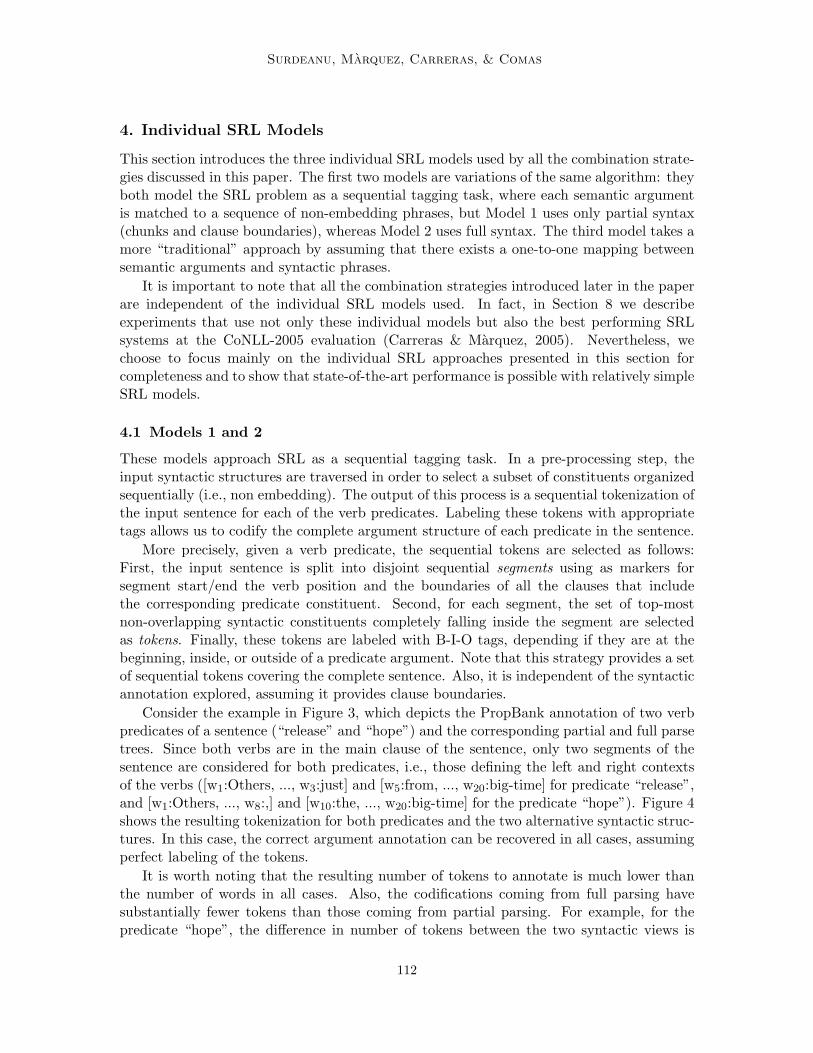
4. Individual SRL Models
This section introduces the three individual SRL models used by all the combination strate-gies discussed in this paper. The first two models are variations of the same algorithm: theyboth model the SRL problem as a sequential tagging task, where each semantic argumentis matched to a sequence of non-embedding phrases, but Model 1 uses only partial syntax(chunks and clause boundaries), whereas Model 2 uses full syntax. The third model takes amore “traditional” approach by assuming that there exists a one-to-one mapping betweensemantic arguments and syntactic phrases.
It is important to note that all the combination strategies introduced later in the paperare independent of the individual SRL models used. In fact, in Section 8 we describeexperiments that use not only these individual models but also the best performing SRLsystems at the CoNLL-2005 evaluation (Carreras & Marquez, 2005). Nevertheless, wechoose to focus mainly on the individual SRL approaches presented in this section forcompleteness and to show that state-of-the-art performance is possible with relatively simpleSRL models.
4.1 Models 1 and 2
These models approach SRL as a sequential tagging task. In a pre-processing step, theinput syntactic structures are traversed in order to select a subset of constituents organizedsequentially (i.e., non embedding). The output of this process is a sequential tokenization ofthe input sentence for each of the verb predicates. Labeling these tokens with appropriatetags allows us to codify the complete argument structure of each predicate in the sentence.
More precisely, given a verb predicate, the sequential tokens are selected as follows:First, the input sentence is split into disjoint sequential segments using as markers forsegment start/end the verb position and the boundaries of all the clauses that includethe corresponding predicate constituent. Second, for each segment, the set of top-mostnon-overlapping syntactic constituents completely falling inside the segment are selectedas tokens. Finally, these tokens are labeled with B-I-O tags, depending if they are at thebeginning, inside, or outside of a predicate argument. Note that this strategy provides a setof sequential tokens covering the complete sentence. Also, it is independent of the syntacticannotation explored, assuming it provides clause boundaries.
Consider the example in Figure 3, which depicts the PropBank annotation of two verbpredicates of a sentence (“release” and “hope”) and the corresponding partial and full parsetrees. Since both verbs are in the main clause of the sentence, only two segments of thesentence are considered for both predicates, i.e., those defining the left and right contextsof the verbs ([w1:Others, ..., w3:just] and [w5:from, ..., w20:big-time] for predicate “release”,and [w1:Others, ..., w8:,] and [w10:the, ..., w20:big-time] for the predicate “hope”). Figure 4shows the resulting tokenization for both predicates and the two alternative syntactic struc-tures. In this case, the correct argument annotation can be recovered in all cases, assumingperfect labeling of the tokens.
It is worth noting that the resulting number of tokens to annotate is much lower thanthe number of words in all cases. Also, the codifications coming from full parsing havesubstantially fewer tokens than those coming from partial parsing. For example, for thepredicate “hope”, the difference in number of tokens between the two syntactic views is
112

Combination Strategies for Semantic Role Labeling
the senior league will be their bridge into the big−time.hope back,fromreleasedjustOthers the majors,
the senior league will be their bridge into the big−time.hope back,fromreleasedjustOthers the majors,
P A1
A2
A0
AM−TMP PA1
IIClause
6VP
INP
4PP
1NP
3ADVP
, ,
Clause
NP VP
VP
52
NP3ADVP
II,
IVVP
4 VPP
5 VINP
6 VII,
7VP
8 VIIIClause
1
2
IIIINPPPNPVP
Clause
NP ADVP
Figure 3: Annotation of an example sentence with two alternative syntactic structures. Thelower tree corresponds to a partial parsing annotation (PP) with base chunks andclause structure, while the upper represents a full parse tree (FP). Semantic rolesfor two predicates (“release” and “hope”) are also provided for the sentence. Theencircled nodes in both trees correspond to the selected nodes by the processof sequential tokenization of the sentence. We mark the selected nodes for thepredicate “release” with Western numerals and the nodes selected for “hope” withRoman numerals. See Figure 4 for more details.
particularly large (8 vs. 2 tokens). Obviously, the coarser the token granularity, the easierthe problem of assigning correct output labelings (i.e., there are less tokens to label andalso the long-distance relations among sentence constituents can be better captured). Onthe other hand, a coarser granularity tends to introduce more unrecoverable errors in thepre-processing stage. There is a clear trade-off, which is difficult to solve in advance. Byusing the two models in a combination scheme we can take advantage of the diverse sentencetokenizations (see Sections 7 and 8).
Compared to the more common tree node labeling approaches (e.g., the followingModel 3), the B-I-O annotation of tokens has the advantage of permitting to correctly an-notate some arguments that do not match a unique syntactic constituent. On the bad side,the heuristic pre-selection of only some candidate nodes for each predicate, i.e., the nodesthat sequentially cover the sentence, makes the number of unrecoverable errors higher. An-other source of errors common to all strategies are the errors introduced by real partial/fullparsers. We have calculated that due to syntactic errors introduced in the pre-processingstage, the upper-bound recall figures are 95.67% for Model 1 and 90.32% for Model 2 usingthe datasets defined in Section 8.
113

Surdeanu, Marquez, Carreras, & Comas
tokenswords release–PP release–FP hope–PP hope–FP1: Others 1: B A1 1: B A1 I: B A0
2: , 2: O 2: O II: I A0
3: just 3: B AM-TMP 3: B AM-TMP III: I A0
4: released — — IV: I A0 I: B A0
5: from 4: B A2 V: I A0
6: the 5: I A2 4: B A2 VI: I A0
7: majors8: , 6: O 5: O VII: I A0
9: hope 7: O — —
10: the11: senior12: league13: will14: be 6: O15: their 8: O VIII: B A1 II: B A1
16: bridge17: back18: into19: the20: big-time
Figure 4: Sequential tokenization of the sentence in Figure 3 according to the two syntacticviews and predicates (PP stands for partial parsing and FP for full parsing). Thesentence and semantic role annotations are vertically displayed. Each token isnumbered with the indexes that appear in the tree nodes of Figure 3 and containsthe B-I-O annotation needed to codify the proper semantic role structure.
Approaching SRL as a sequential tagging task is not new. Hacioglu, Pradhan, Ward,Martin, and Jurafsky (2004) presented a system based on sequential tagging of base chunkswith B-I-O labels, which was the best performing SRL system at the CoNLL-2004 sharedtask (Carreras & Marquez, 2004). The novelty of our approach resides in the fact that thesequence of syntactic tokens to label is extracted from a hierarchical syntactic annotation(either a partial or a full parse tree) and it is not restricted to base chunks (i.e., a tokenmay correspond to a complex syntactic phrase or even a clause).
4.1.1 Features
Once the tokens selected are labeled with B-I-O tags, they are converted into trainingexamples by considering a rich set of features, mainly borrowed from state-of-the-art sys-tems (Gildea & Jurafsky, 2002; Carreras, Marquez, & Chrupa�la, 2004; Xue & Palmer,2004). These features codify properties from: (a) the focus token, (b) the target predicate,(c) the sentence fragment between the token and predicate, and (d) the dynamic context,i.e., B-I-O labels previously generated. We describe these four feature sets next.2
2. Features extracted from partial parsing and Named Entities are common to Model 1 and 2, while featurescoming from full parse trees only apply to Model 2.
114

Combination Strategies for Semantic Role Labeling
Constituent structure features:
• Constituent type and head: extracted using the head-word rules of Collins (1999).If the first element is a PP chunk, then the head of the first NP is extracted. Forexample, the type of the constituent “in the U.S.” in Figure 1 is PP, but its head is“U.S.” instead of “in”.
• First and last words and POS tags of the constituent, e.g., “in”/IN and “U.S.”/NNPfor the constituent “in the U.S.” in Figure 1.
• POS sequence: if it is less than 5 tags long, e.g., IN−DT−NNP for the above sampleconstituent.
• 2/3/4-grams of the POS sequence.
• Bag-of-words of nouns, adjectives, and adverbs. For example, the bag-of-nouns forthe constituent “The luxury auto maker” is {“luxury”, “auto”, “maker”}.
• TOP sequence: sequence of types of the top-most syntactic elements in the constituent(if it is less than 5 elements long). In the case of full parsing this corresponds to theright-hand side of the rule expanding the constituent node. For example, the TOPsequence for the constituent “in the U.S.” is IN−NP.
• 2/3/4-grams of the TOP sequence.
• Governing category as described by Gildea and Jurafsky (2002), which indicates if NParguments are dominated by a sentence (typical for subjects) or a verb phrase (typicalfor objects). For example, the governing category for the constituent “1,214 cars” inFigure 1 is VP, which hints that its corresponding semantic role will be object.
• NamedEntity, indicating if the constituent embeds or strictly matches a named entityalong with its type. For example, the constituent “in the U.S.” embeds a locativenamed entity: “U.S.”.
• TMP, indicating if the constituent embeds or strictly matches a temporal keyword(automatically extracted from AM-TMP arguments of the training set). Among the mostcommon temporal cue words extracted are: “year”, “yesterday”, “week”, “month”,etc. We used a total of 109 cue words.
• Previous and following words and POS tag of the constituent. For example, theprevious word for the constituent “last year” in Figure 1 is “maker”/NN, and the nextone is “sold”/VBD.
• The same features characterizing focus constituents are extracted for the two previousand following tokens, provided they are inside the boundaries of the current segment.
Predicate structure features:
• Predicate form, lemma, and POS tag, e.g., “sold”, “sell”, and VBD for the predicate inFigure 1.
• Chunk type and cardinality of verb phrase in which verb is included: single-word ormulti-word. For example, the predicate in Figure 1 is included in a single-word VP
chunk.
115

Surdeanu, Marquez, Carreras, & Comas
• The predicate voice. We distinguish five voice types: active, passive, copulative,infinitive, and progressive.
• Binary flag indicating if the verb is a start/end of a clause.
• Sub-categorization rule, i.e., the phrase structure rule that expands the predicate’simmediate parent, e.g., S → NP NP VP for the predicate in Figure 1.
Predicate-constituent features:
• Relative position, distance in words and chunks, and level of embedding (in number ofclause-levels) with respect to the constituent. For example, the constituent “in theU.S.” in Figure 1 appears after the predicate, at a distance of 2 words or 1 chunk,and its level of embedding is 0.
• Constituent path as described by Gildea and Jurafsky (2002) and all 3/4/5-grams ofpath constituents beginning at the verb predicate or ending at the constituent. Forexample, the syntactic path between the constituent “The luxury auto maker” andthe predicate “sold” in Figure 1 is NP ↑ S ↓ VP ↓ VBD.
• Partial parsing path as described by Carreras et al. (2004) and all 3/4/5-grams of pathelements beginning at the verb predicate or ending at the constituent. For example,the path NP + PP + NP + S ↓ VP ↓ VBD indicates that from the current NP tokento the predicate there are PP, NP, and S constituents to the right (positive sign) atthe same level of the token and then the path descends through the clause and a VPto find the predicate. The difference from the previous constituent path is that we donot have up arrows anymore but we introduce “horizontal” (left/right) movements atthe same syntactic level.
• Syntactic frame as described by Xue and Palmer (2004). The syntactic frame capturesthe overall sentence structure using the predicate and the constituent as pivots. Forexample, the syntactic frame for the predicate “sold” and the constituent “in theU.S.” is NP−NP−VP−NP−PP, with the current predicate and constituent emphasized.Knowing that there are other noun phrases before the predicate lowers the probabilitythat this constituent serves as an agent (or A0).
Dynamic features:
• BIO–tag of the previous token. When training, the correct labels of the left contextare used. When testing, this feature is dynamically codified as the tag previouslyassigned by the SRL tagger.
4.1.2 Learning Algorithm and Sequence Tagging
We used generalized AdaBoost with real-valued weak classifiers (Schapire & Singer, 1999) asthe base learning algorithm. Our version of the algorithm learns fixed-depth small decisiontrees as weak rules, which are then combined in the ensemble constructed by AdaBoost.We implemented a simple one-vs-all decomposition to address multi-class classification. Inthis way, a separate binary classifier has to be learned for each B-X and I-X argument labelplus an extra classifier for the O decision.
116

Combination Strategies for Semantic Role Labeling
AdaBoost binary classifiers are then used for labeling test sequences, from left to right,using a recurrent sliding window approach with information about the tags assigned to thepreceding tokens. As explained in the previous list of features, left tags already assignedare dynamically codified as features. Empirically, we found that the optimal left context tobe taken into account reduces to only the previous token.
We tested two different tagging procedures. First, a greedy left-to-right assignment ofthe best scored label for each token. Second, a Viterbi search of the label sequence thatmaximizes the probability of the complete sequence. In this case, the classifiers’ predictionswere converted into probabilities using the softmax function described in Section 7.1. Nosignificant improvements were obtained from the latter. We selected the former, which isfaster, as our basic tagging algorithm for the experiments.
Finally, this tagging model enforces three basic constraints: (a) the B-I-O output label-ing must codify a correct structure; (b) arguments cannot overlap with clause nor chunkboundaries; and (c) for each verb, A0-5 arguments not present in PropBank frames (takingthe union of all rolesets for the different verb senses) are not considered.
4.2 Model 3
The third individual SRL model makes the strong assumption that each predicate argumentmaps to one syntactic constituent. For example, in Figure 1 A0 maps to a noun phrase,AM-LOC maps to a prepositional phrase, etc. This assumption holds well on hand-correctedparse trees and simplifies significantly the SRL process because only one syntactic con-stituent has to be correctly classified in order to recognize one semantic argument. On theother hand, this approach is limited when using automatically-generated syntactic trees. Forexample, only 91.36% of the arguments can be mapped to one of the syntactic constituentsproduced by the Charniak parser.
Using a bottom-up approach, Model 3 maps each argument to the first syntactic con-stituent that has the exact same boundaries and then climbs as high as possible in thetree across unary production chains. We currently ignore all arguments that do not mapto a single syntactic constituent. The argument-constituent mapping is performed on thetraining set as preprocessing step. Figure 1 shows a mapping example between the semanticarguments of one verb and the corresponding sentence syntactic structure.
Once the mapping process completes, Model 3 extracts a rich set of lexical, syntactic,and semantic features. Most of these features are inspired from previous work in parsingand SRL (Collins, 1999; Gildea & Jurafsky, 2002; Surdeanu et al., 2003; Pradhan et al.,2005a). We describe the complete feature set implemented in Model 3 next.
4.2.1 Features
Similarly to Models 1 and 2 we group the features in three categories, based on the propertiesthey codify: (a) the argument constituent, (b) the target predicate, and (c) the relationbetween the constituent and predicate syntactic constituents.
Constituent structure features:
• The syntactic label of the candidate constituent.
• The constituent head word, suffixes of length 2, 3, and 4, lemma, and POS tag.
117

Surdeanu, Marquez, Carreras, & Comas
• The constituent content word, suffixes of length 2, 3, and 4, lemma, POS tag, and NElabel. Content words, which add informative lexicalized information different from thehead word, were detected using the heuristics of Surdeanu et al. (2003). For example,the head word of the verb phrase “had placed” is the auxiliary verb “had”, whereasthe content word is “placed”. Similarly, the content word of prepositional phrases isnot the preposition itself (which is selected as the head word), but rather the headword of the attached phrase, e.g., “U.S.” for the prepositional phrase “in the U.S.”.
• The first and last constituent words and their POS tags.
• NE labels included in the candidate phrase.
• Binary features to indicate the presence of temporal cue words, i.e., words that appearoften in AM-TMP phrases in training. We used the same list of temporal cue words asModels 1 and 2.
• For each Treebank syntactic label we added a feature to indicate the number of suchlabels included in the candidate phrase.
• The TOP sequence of the constituent (constructed similarly to Model 2).
• The phrase label, head word and POS tag of the constituent parent, left sibling, andright sibling.
Predicate structure features:
• The predicate word and lemma.
• The predicate voice. Same definition as Models 1 and 2.
• A binary feature to indicate if the predicate is frequent (i.e., it appears more thantwice in the training data) or not.
• Sub-categorization rule. Same definition as Models 1 and 2.
Predicate-constituent features:
• The path in the syntactic tree between the argument phrase and the predicate asa chain of syntactic labels along with the traversal direction (up or down). It iscomputed similarly to Model 2.
• The length of the above syntactic path.
• The number of clauses (S* phrases) in the path. We store the overall clause countand also the number of clauses in the ascending and descending part of the path.
• The number of verb phrases (VP) in the path. Similarly to the above feature, we storethree numbers: overall verb count, and the verb count in the ascending/descendingpart of the path.
• Generalized syntactic paths. We generalize the path in the syntactic tree, when itappears with more than 3 elements, using two templates: (a) Arg ↑ Ancestor ↓ Ni ↓Pred, where Arg is the argument label, Pred is the predicate label, Ancestor is thelabel of the common ancestor, and Ni is instantiated with each of the labels between
118

Combination Strategies for Semantic Role Labeling
Pred and Ancestor in the full path; and (b) Arg ↑ Ni ↑ Ancestor ↓ Pred, where Ni isinstantiated with each of the labels between Arg and Ancestor in the full path. Forexample, in the path NP ↑ S ↓ VP ↓ SBAR ↓ S ↓ VP the argument label is the first NP, thepredicate label is the last VP, and the common ancestor’s label is the first S. Hence,using the last template, this path is generalized to the following three features: NP ↑S ↓ VP ↓ VP, NP ↑ S ↓ SBAR ↓ VP, and NP ↑ S ↓ S ↓ VP. This generalization reduces thesparsity of the complete constituent-predicate path feature using a different strategythan Models 1 and 2, which implement a n-gram based approach.
• The subsumption count, i.e., the difference between the depths in the syntactic treeof the argument and predicate constituents. This value is 0 if the two phrases sharethe same parent.
• The governing category, similar to Models 1 and 2.
• The surface distance between the predicate and the argument phrases encoded as:the number of tokens, verb terminals (VB*), commas, and coordinations (CC) be-tween the argument and predicate phrases, and a binary feature to indicate if the twoconstituents are adjacent. For example, the surface distance between the argumentcandidate “Others” and the predicate “hope” in the Figure 3 example: “Others, justreleased from the majors, hope the senior league...” is 7 tokens, 1 verb, 2 commas,and 0 coordinations. These features, originally proposed by Collins (1999) for his de-pendency parsing model, capture robust, syntax-independent information about thesentence structure. For example, a constituent is unlikely to be the argument of averb if another verb appears between the two phrases.
• A binary feature to indicate if the argument starts with a predicate particle, i.e., atoken seen with the RP* POS tag and directly attached to the predicate in training.The motivation for this feature is to avoid the inclusion of predicate particles in theargument constituent. For example, without this feature, a SRL system will tend toincorrectly include the predicate particle in the argument for the text: “take [A1overthe organization]”, because the marked text is commonly incorrectly parsed as aprepositional phrase and a large number of prepositional phrases directly attached toa verb are arguments for the corresponding predicate.
4.2.2 Classifier
Similarly to Models 1 and 2, Model 3 trains one-vs-all classifiers using AdaBoost for the mostcommon argument labels. To reduce the sample space, Model 3 selects training examples(both positive and negative) only from: (a) the first clause that includes the predicate, or(b) from phrases that appear to the left of the predicate in the sentence. More than 98%of the argument constituents fall into one of these classes.
At prediction time the classifiers are combined using a simple greedy technique thatiteratively assigns to each predicate the argument classified with the highest confidence. Foreach predicate we consider as candidates all AM attributes, but only numbered attributesindicated in the corresponding PropBank frame. Additionally, this greedy strategy enforcesa limited number of domain knowledge constraints in the generated solution: (a) argumentscan not overlap in any form, (b) no duplicate arguments are allowed for A0-5, and (c) each
119

Surdeanu, Marquez, Carreras, & Comas
predicate can have numbered arguments, i.e., A0-5, only from the subset present in itsPropBank frame. These constraints are somewhat different from the constraints used byModels 1 and 2: (i) Model 3 does not use the B-I-O representation hence the constraintthat the B-I-O labeling be correct does not apply; and (ii) Models 1 and 2 do not enforcethe constraint that numbered arguments can not be duplicated because its implementationis not straightforward in this architecture.
5. Performance of the Individual Models
In this section we analyze the performance of the three individual SRL models proposed.Our three SRL systems were trained using the complete CoNLL-2005 training set (Prop-Bank/Treebank sections 2 to 21). To avoid the overfitting of the syntactic processors −i.e.,part-of-speech tagger, chunker, and Charniak’s full parser− we partitioned the PropBanktraining set into five folds and for each fold we used the output of the syntactic processorsthat were trained on the other four folds. The models were tuned on a separate develop-ment partition (Treebank section 24) and evaluated on two corpora: (a) Treebank section23, which consists of Wall Street Journal (WSJ) documents, and (b) on three sections of theBrown corpus, semantically annotated by the PropBank team for the CoNLL-2005 sharedtask evaluation.
All the classifiers for our individual models were developed using AdaBoost with de-cision trees of depth 4 (i.e., each branch may represent a conjunction of at most 4 basicfeatures). Each classification model was trained for up to 2,000 rounds. We applied somesimplifications to keep training times and memory requirements inside admissible bounds:(a) we have trained only the most frequent argument labels: top 41 for Model 1, top 35for Model 2, and top 24 for Model 3; (b) we discarded all features occurring less than 15times in the training set, and (c) for each Model 3 classifier, we have limited the number ofnegative training samples to the first 500,000 negative samples extracted in the PropBanktraversal3.
Table 1 summarizes the results of the three models on the WSJ and Brown corpora.We include the percentage of perfect propositions detected by each model (“PProps”),i.e., predicates recognized with all their arguments, the overall precision, recall, and F1
measure4. The results summarized in Table 1 indicate that all individual systems havea solid performance. Although none of them would rank in the top 3 in the CoNLL-2005 evaluation (Carreras & Marquez, 2005), their performance is comparable to the bestindividual systems presented at that evaluation exercise5. Consistently with other systemsevaluated on the Brown corpus, all our models experience a severe performance drop in thiscorpus, due to the lower performance of the linguistic processors.
As expected, the models based on full parsing (2 and 3) perform better than the modelbased on partial syntax. But, interestingly, the difference is not large (e.g., less than 2 points
3. The distribution of samples for the Model 3 classifiers is very biased towards negative samples because, inthe worst case, any syntactic constituent in the same sentence with the predicate is a potential argument.
4. The significance intervals for the F1 measure have been obtained using bootstrap resampling (Noreen,1989). F1 rates outside of these intervals are assumed to be significantly different from the related F1
rate (p < 0.05).5. The best performing SRL systems at CoNLL were a combination of several subsystems. See section 9
for details.
120

Combination Strategies for Semantic Role Labeling
WSJ PProps Precision Recall F1
Model 1 48.45% 78.76% 72.44% 75.47 ±0.8
Model 2 52.04% 79.65% 74.92% 77.21 ±0.8
Model 3 45.28% 80.32% 72.95% 76.46 ±0.6
Brown
Model 1 30.85% 67.72% 58.29% 62.65 ±2.1
Model 2 36.44% 71.82% 64.03% 67.70 ±1.9
Model 3 29.48% 72.41% 59.67% 65.42 ±2.1
Table 1: Overall results of the individual models in the WSJ and Brown test sets.
A0 A1 A2 A3 A4
Model 1 F1 83.37 75.13 67.33 61.92 72.73Model 2 F1 86.65 77.06 65.04 62.72 72.43Model 3 F1 86.14 75.83 65.55 65.26 73.85
Table 2: F1 scores of the individual systems for the A0−4 arguments in the WSJ test.
in F1 in the WSJ corpus), evincing that having base syntactic chunks and clause boundariesis enough to obtain competitive performance. More importantly, the full-parsing models arenot always better than the partial-syntax model. Table 2 lists the F1 measure for the threemodels for the first five numbered arguments. Table 2 shows that Model 2, our overallbest performing individual system, achieves the best F-measure for A0 and A1 (typicallysubjects and direct objects), but Model 1, the partial-syntax model, performs best forthe A2 (typically indirect objects, instruments, or benefactives). The explanation for thisbehavior is that indirect objects tend to be farther from their predicates and accumulatemore parsing errors. From the models based on full syntax, Model 2 has better recallwhereas Model 3 has better precision, because Model 3 filters out all candidate argumentsthat do not match a single syntactic constituent. Generally, Table 2 shows that all modelshave strong and weak points. This is further justification for our focus on combinationstrategies that combine several independent models.
6. Features of the Combination Models
As detailed in Section 3, in this paper we analyze two classes of combination strategies forthe problem of semantic role labeling: (a) an inference model with constraint satisfaction,which finds the set of candidate arguments that maximizes a global cost function, and (b)two inference strategies based on learning, where candidates are scored and ranked usingdiscriminative classifiers. From the perspective of the feature space, the main differencebetween these two types of combination models is that the input of the first combina-tion strategy is limited to the argument probabilities produced by the individual systems,whereas the last class of combination approaches incorporates a much larger feature set intheir ranking classifiers. For robustness, in this paper we use only features that are ex-tracted from the solutions provided by the individual systems, hence are independent of the
121

Surdeanu, Marquez, Carreras, & Comas
������������������������
������������������������
������������
������������
��������������������������������
��������������������������������
A1
V
A2
V
A1
A4
V
A1
M2 M3M1
A0
A0
Figure 5: Sample solutions proposed for the same predicate by three individual SRL models:M1, M2 and M3. Argument candidates are displayed vertically for each system.
individual models6. We describe all these features next. All examples given in this sectionare based on Figures 5 and 6.
Voting features − these features quantify the votes received by each argument from theindividual systems. This set includes the following features:
• The label of the candidate argument, e.g., A0 for the first argument proposed by systemM1 in Figure 5.
• The number of systems that generated an argument with this label and span. For theexample shown in Figure 5, this feature has value 1 for the argument A0 proposed byM1 and 2 for M1’s A1, because system M2 proposed the same argument.
• The unique ids of all the systems that generated an argument with this label andspan, e.g., M1 and M2 for the argument A1 proposed by M1 or M2 in Figure 5.
• The argument sequence for this predicate for all the systems that generated an ar-gument with this label and span. For example, the argument sequence generated bysystem M1 for the proposition illustrated in Figure 5 is: A0 - V - A1 - A2. This fea-ture attempts to capture information at proposition level, e.g., a combination modelmight learn to trust model M1 more for the argument sequence A0 - V - A1 - A2,M2 for another sequence, etc.
Same-predicate overlap features − these features measure the overlap between differentarguments produced by the individual SRL models for the same predicate:
6. With the exception of the argument probabilities, which are required by the constraint satisfaction model.
122

Combination Strategies for Semantic Role Labeling
• The number and unique ids of all the systems that generated an argument with thesame span but different label. For the example shown in Figure 5, these features havevalues 1 and M2 for the argument A2 proposed by M1, because model M2 proposedargument A4 with the same span.
• The number and unique ids of all the systems that generated an argument includedin the current argument. For the candidate argument A0 proposed by model M1 inFigure 5, these features have values 1 and M3, because M3 generated argument A0,which is included in M1’s A0.
• In the same spirit, we generate the number and unique ids of all the systems thatgenerated an argument that contains the current argument, and the number andunique ids of all the systems that generated an argument that overlaps − but doesnot include nor contain − the current argument.
Other-predicate overlap features − these features quantify the overlap between differ-ent arguments produced by the individual SRL models for other predicates. We generate thesame features as the previous feature group, with the difference that we now compare argu-ments generated for different predicates. The motivation for these overlap features is that,according to the PropBank annotations, no form of overlap is allowed among argumentsattached to the same predicate, and only inclusion or containment is permitted betweenarguments assigned to different predicates. The overlap features are meant to detect whenthese domain constraints are not satisfied by a candidate argument, which is an indication,if the evidence is strong, that the candidate is incorrect.
Partial-syntax features − these features codify the structure of the argument and thedistance between the argument and the predicate using only partial syntactic information,i.e., chunks and clause boundaries (see Figure 6 for an example). Note that these featuresare inherently different from the features used by Model 1, because Model 1 evaluates eachindividual chunk part of a candidate argument, whereas here we codify properties of thecomplete argument constituent. We describe the partial-syntax features below.
• Length in tokens and chunks of the argument constituent, e.g., 4 and 1 for argumentA0 in Figure 6.
• The sequence of chunks included in the argument constituent, e.g., PP NP for theargument AM-LOC in Figure 6. If the chunk sequence is too large, we store n-grams oflength 10 for the start and end of the sequence.
• The sequence of clause boundaries, i.e., clause beginning or ending, included in theargument constituent.
• The named entity types included in the argument constituent, e.g., LOCATION for theAM-LOC argument in Figure 6.
• Position of the argument: before/after the predicate in the sentence, e.g., after for A1in Figure 6.
• A Boolean flag to indicate if the argument constituent is adjacent to the predicate,e.g., false for A0 and true for A1 in Figure 6.
123

Surdeanu, Marquez, Carreras, & Comas
The luxury auto maker last year sold 1,214 cars
PA0 AM−TMP A1 AM−LOC
the U.S.in
NP NP VP NP PP NP
Clause
Figure 6: Sample proposition with partial syntactic information.
• The sequence of chunks between the argument constituent and the predicate, e.g., thechunk sequence between the predicate and the argument AM-LOC in Figure 6 is: NP.Similarly to the above chunk sequence feature, if the sequence is too large, we storestarting and ending n-grams.
• The number of chunks between the predicate and the argument, e.g., 1 for AM-LOC inFigure 6.
• The sequence of clause boundaries between the argument constituent and the predicate.
• The clause subsumption count, i.e., the difference between the depths in the clausetree of the argument and predicate constituents. This value is 0 if the two phrases areincluded in the same clause.
Full-syntax features − these features codify the structure of the argument constituent,the predicate, and the distance between the two using full syntactic information. Thefull-syntax features are replicated from Model 3 (see Section 4.2), which assumes that aone-to-one mapping from semantic constituents to syntactic phrases exists. Unlike Model 3which ignores arguments that can not be matched against a syntactic constituent, if suchan exact mapping does not exist due to the inclusion of candidates from Models 1 and 2, wegenerate an approximate mapping from the unmapped semantic constituent to the largestphrase that is included in the given span and has the same left boundary as the seman-tic constituent. This heuristic guarantees that we capture at least some of the semanticconstituents’ syntactic structure.
The motivation for the partial and full-syntax features is to learn the “preferences” ofthe individual SRL models. For example, with these features a combination classifier mightlearn to trust model M1 for arguments that are closer than 3 chunks to the predicate, modelM2 when the predicate-argument syntactic path is NP ↑ S ↓ VP ↓ SBAR ↓ S ↓ VP, etc.
Individual systems’ argument probabilities − each individual model outputs a con-fidence score for each of their proposed arguments. These scores are converted into prob-abilities using the softmax function as described in detail in Section 7.1. The combinationstrategy based on constraint satisfaction (Section 7.1) uses these probabilities as they are,while the other two strategies based on meta-learning (Section 7.2) have to discretize theprobabilities to include them as features. To do so, each probability value is matched to
124

Combination Strategies for Semantic Role Labeling
one of five probability intervals and the corresponding interval is used as the feature. Theprobability intervals are dynamically constructed for each argument label and each indi-vidual system such that the corresponding system predictions for this argument label areuniformly distributed across the intervals.
In Section 8.4 we empirically analyze the contribution of each of these proposed featuresets to the performance of our best combination model.
7. Combination Strategies
In this section we detail the combination strategies proposed in this paper: (a) a combinationmodel with constraint satisfaction, which aims at finding the set of candidate argumentsthat maximizes a global cost function, and (b) two combination models with inference basedon learning, where candidates are scored and ranked using discriminative classifiers. In theprevious section we described the complete feature set made available to all approaches.Here we focus on the machine learning paradigm deployed by each of the combinationmodels.
7.1 Inference with Constraint Satisfaction
The Constraint Satisfaction model selects a subset of candidate arguments that maximizesa compatibility function subject to the fulfillment of a set of structural constraints thatensure consistency of the solution. The compatibility function is based on the probabilitiesgiven by individual SRL models to the candidate arguments. In this work we use IntegerLinear Programming to solve the constraint satisfaction problem. This approach was firstproposed by Roth and Yih (2004) and applied to semantic role labeling by Punyakanok,Roth, Yih, and Zimak (2004), Koomen et al. (2005), among others. We follow the settingof Komen et al., which is taken as a reference.
As a first step, the scores from each model are normalized into probabilities. The scoresyielded by the classifiers are signed and unbounded real numbers, but experimental evidenceshows that the confidence in the predictions (taken as the absolute value of the raw scores)correlates well with the classification accuracy. Thus, the softmax function (Bishop, 1995)is used to convert the set of unbounded scores into probabilities. If there are k possibleoutput labels for a given argument and sco(li) denotes the score of label li output by afixed SRL model, then the estimated probability for this label is:
p(li) =eγsco(li)
∑kj=1 eγsco(lj)
The γ parameter of the above formula can be empirically adjusted to avoid overly skewedprobability distributions and to normalize the scores of the three individual models to asimilar range of values. See more details about our experimental setting in Section 8.1.
Candidate selection is performed via Integer Linear Programming (ILP). The programgoal is to maximize a compatibility function modeling the global confidence of the selectedset of candidates, subject to a set of linear constraints. All the variables involved in thetask take integer values and may appear in first degree polynomials only.
An abstract ILP process can be described in a simple fashion as: given a set of vari-ables V = {v1, . . . , vn}, it aims to maximize the global compatibility of a label assignment
125

Surdeanu, Marquez, Carreras, & Comas
{l1, . . . , ln} to these variables. A local compatibility function cv(l) defines the compatibilityof assigning label l to variable v. The global compatibility function C(l1, . . . , ln) is takenas the sum of each local assignment compatibility, so the goal of the ILP process can bewritten as:
argmaxl1,...,ln
C(l1, . . . , ln) = argmaxl1,...,ln
n∑
i=1
cvi(li)
where the constraints are described in a set of accompanying integer linear equations in-volving the variables of the problem.
If one wants to codify soft constraints instead of hard, there is the possibility of consider-ing them as a penalty component in the compatibility function. In this case, each constraintr ∈ R can be seen as a function which takes the current label assignment and outputs areal number, which is 0 when the constraint is satisfied and a positive number when not,indicating the penalty imposed to the compatibility function. The new expression of thecompatibility function to maximize is:
C(l1, . . . , ln) =n∑
i=1
cvi(li)−
∑
r∈R
r(l1, . . . , ln)
Note that the hard constraints can also be simulated in this setting by making them outputa very large positive number when they are violated.
In our particular problem, we have a binary-valued variable vi for each of the N argu-ment candidates generated by the SRL models, i.e., li labels are in {0, 1}. Given a labelassignment, the arguments with li = 1 are selected to form the solution, while the others(those where li = 0) are filtered out. For each variable vi, we also have the probabilityvalues, pij , calculated from the score of model j on argument i, according to the softmaxformula described above7. In a first approach, the compatibility function cv(li) equals to(∑M
j=1 pij)li, where the number of models, M , is 3 in our case8.Under this definition, maximizing the compatibility function is equivalent to maximizing
the sum of the probabilities given by the models to the argument candidates considered inthe solution. Since this function is always positive, the global score increases directly withthe number of selected candidates. As a consequence, the model is biased towards themaximization of the number of candidates included in the solution (e.g., tending to selecta lot of small non-overlapping arguments). Following Koomen et al. (2005), this bias canbe corrected by adding a new score oi, which sums to the compatibility function when thei-th candidate is not selected in the solution. The global compatibility function needs to berewritten to encompass this new information. Formalized as an ILP equation, it looks like:
argmaxL∈{0,1}N
C(l1, . . . , lN ) = argmaxL∈{0,1}N
N∑
i=1
(M∑
j=1
pij)li + oi(1− li)
7. If model j does not propose argument i then we consider pij = 0.8. Instead of accumulating the probabilities of all models for a given candidate argument, one could consider
a different variable for each model prediction and introduce a constraint forcing all these variables totake the same value at the end of the optimization problem. The two alternatives are equivalent.
126

Combination Strategies for Semantic Role Labeling
where the constraints are expressed in separated integer linear equations. It is not possibleto define a priori the value of oi. Komen et al. used a validation corpus to empiricallyestimate a constant value for all oi (i.e., independent from the argument candidate)9. Wewill use exactly the same solution of working with a single constant value, to which we willrefer as O.
Regarding the consistency constraints, we have considered the following six:
1. Two candidate arguments for the same verb can not overlap nor embed.
2. A verb may not have two core arguments with the same type label A0-A5.
3. If there is an argument R-X for a verb, there has to be also an X argument for thesame verb.
4. If there is an argument C-X for a verb, there has to be also an X argument before theC-X for the same verb.
5. Arguments from two different verbs can not overlap, but they can embed.
6. Two different verbs can not share the same AM-X, R-AM-X or C-X arguments.
Constraints 1–4 are also included in our reference work (Punyakanok et al., 2004). Noother constraints from that paper need to be checked here since each individual modeloutputs only consistent solutions. Constraints 5 and 6, which restrict the set of compatiblearguments among different predicates in the sentence, are original to this work. In theInteger Linear Programming setting the constraints are written as inequalities. For example,if Ai is the argument label of the i-th candidate and Vi its verb predicate, constraint number2 is written as:
∑(Ai=a∧Vi=v) li ≤ 1, for a given verb v and argument label a. The other
constraints have similar translations into inequalities.
Constraint satisfaction optimization will be applied in two different ways to obtainthe complete output annotation of a sentence. In the first one, we proceed verb by verbindependently to find their best selection of candidate arguments using only constraints1 through 4. We call this approach local optimization. In the second scenario all thecandidate arguments in the sentence are considered at once and constraints 1 through 6 areenforced. We will refer to this second strategy as global optimization. In both scenarios thecompatibility function will be the same, but constraints need some rewriting in the globalscenario because they have to include information about the concrete predicate.
In Section 8.3 we will extensively evaluate the presented inference model based on Con-straint Satisfaction, and we will describe some experiments covering the following topics: (a)the contribution of each of the proposed constraints; (b) the performance of local vs. globaloptimization; and (c) the precision–recall tradeoff by varying the value of the bias-correctionparameter.
7.2 Inference Based On Learning
This combination model consists of two stages: a candidate scoring phase, which scorescandidate arguments in the pool using a series of discriminative classifiers, and an inferencestage, which selects the best overall solution that is consistent with the domain constraints.
9. Instead of working with a constant, one could try to set the oi value for each candidate, taking intoaccount some contextual features of the candidate. We plan to explore this option in the near future.
127

Surdeanu, Marquez, Carreras, & Comas
The first and most important component of this combination strategy is the candidatescoring module, which assigns to each candidate argument a score equal to the confidencethat this argument is part of the global solution. It is formed by discriminative functions,one for each role label. Below, we devise two different strategies to train the discriminativefunctions.
After scoring candidate arguments, the final global solution is built by the inferencemodule, which looks for the best scored argument structure that satisfies the domain specificconstraints. Here, a global solution is a subset of candidate arguments, and its score isdefined as the sum of confidence values of the arguments that form it. We currently considerthree constraints to determine which solutions are valid:
(a) Candidate arguments for the same predicate can not overlap nor embed.
(b) In a predicate, no duplicate arguments are allowed for the numbered arguments A0-5.
(c) Arguments of a predicate can be embedded within arguments of other predicates butthey can not overlap.
The set of constraints can be extended with any other rules, but in our particular case, weknow that some constraints, e.g., providing only arguments indicated in the correspond-ing PropBank frame, are already guaranteed by the individual models, and others, e.g.,constraints 3 and 4 in the previous sub-section, have no positive impact on the overallperformance (see Section 8.3 for the empirical analysis). The inference algorithm we useis a bottom-up CKY-based dynamic programming strategy (Younger, 1967). It builds thesolution that maximizes the sum of argument confidences while satisfying the constraints,in cubic time.
Next, we describe two different strategies to train the functions that score candidatearguments. The first is a local strategy: each function is trained as a binary batch classifier,independently of the combination process which enforces the domain constraints. Thesecond is a global strategy: functions are trained as online rankers, taking into account theinteractions that take place during the combination process to decide between one argumentor another.
In both training strategies, the discriminative functions employ the same representa-tion of arguments, using the complete feature set described in Section 6 (we analyze thecontribution of each feature group in Section 8). Our intuition was that the rich featurespace introduced in Section 6 should allow the gathering of sufficient statistics for robustscoring of the candidate arguments. For example, the scoring classifiers might learn thata candidate is to be trusted if: (a) two individual systems proposed it, (b) if its label isA2 and it was generated by Model 1, or (c) if it was proposed by Model 2 within a certainargument sequence.
7.2.1 Learning Local Classifiers
This combination process follows a cascaded architecture, in which the learning componentis decoupled from the inference module. In particular, the training strategy consists oftraining a binary classifier for each role label. The target of each label-based classifier is todetermine whether a candidate argument actually belongs to the correct proposition of thecorresponding predicate, and to output a confidence value for this decision.
128

Combination Strategies for Semantic Role Labeling
The specific training strategy is as follows. The training data consists of a pool oflabeled candidate arguments (proposed by individual systems). Each candidate is eitherpositive, in that it is actually a correct argument of some sentence, or negative, if it isnot correct. The strategy trains a binary classifier for each role label l, independently ofother labels. To do so, it concentrates on the candidate arguments of the data that havelabel l. This forms a dataset for binary classification, specific to the label l. With it, abinary classifier can be trained using any of the existing techniques for binary classification,with the only requirement that our combination strategy needs confidence values with eachbinary prediction. In Section 8 we provide experiments using SVMs to train such localclassifiers.
In all, each classifier is trained independently of other classifiers and the inference mod-ule. Looking globally at the combination process, each classifier can be seen as an argumentfiltering component that decides which candidates are actual arguments using a much richerrepresentation than the individual models. In this context, the inference engine is used as aconflict resolution engine, to ensure that the combined solutions are valid argument struc-tures for sentences.
7.2.2 Learning Global Rankers
This combination process couples learning and inference, i.e., the scoring functions aretrained to behave accurately within the inference module. In other words, the trainingstrategy here is global: the target is to train a global function that maps a set of argumentcandidates for a sentence into a valid argument structure. In our setting, the global functionis a composition of scoring functions −one for each label, same as the previous strategy.Unlike the previous strategy, which is completely decoupled from the inference engine, herethe policy to map a set of candidates into a solution is that determined by the inferenceengine.
In recent years, research has been very active in global learning methods for tagging,parsing and, in general, structure prediction problems (Collins, 2002; Taskar, Guestrin, &Koller, 2003; Taskar, Klein, Collins, Koller, & Manning, 2004; Tsochantaridis, Hofmann,Joachims, & Altun, 2004). In this article, we make use of the simplest technique for globallearning: an online learning approach that uses Perceptron (Collins, 2002). The generalidea of the algorithm is similar to the original Perceptron (Rosenblatt, 1958): correctingthe mistakes of a linear predictor made while visiting training examples, in an additivemanner. The key point for learning global rankers relies on the criteria that determineswhat is a mistake for the function being trained, an idea that has been exploited in asimilar way in multiclass and ranking scenarios by Crammer and Singer (2003a, 2003b).
The Perceptron algorithm in our combination system works as follows (pseudocodeof the algorithm is given in Figure 7). Let 1 . . . L be the possible role labels, and letW = {w1 . . .wL} be the set of parameter vectors of the scoring functions, one for eachlabel. Perceptron initializes the vectors in W to zero, and then proceeds to cycle throughthe training examples, visiting one at a time. In our case, a training example is a pair (y,A),where y is the correct solution of the example and A is the set of candidate arguments forit. Note that both y and A are sets of labeled arguments, and thus we can make use ofthe set difference. We will note as a a particular argument, as l the label of a, and as
129

Surdeanu, Marquez, Carreras, & Comas
Initialization: for each wl ∈ W do wl = 0
Training :
for t = 1 . . . T dofor each training example (y,A) do
y = Inference(A,W)for each a ∈ y \ y do
let l be the label of a
wl = wl + φ(a)for each a ∈ y \ y do
let l be the label of a
wl = wl − φ(a)Output: W
Figure 7: Perceptron Global Learning Algorithm
φ(a) the vector of features described in Section 6. With each example, Perceptron performstwo steps. First, it predicts the optimal solution y according to the current setting ofW. Note that the prediction strategy employs the complete combination model, includingthe inference component. Second, Perceptron corrects the vectors in W according to themistakes seen in y: arguments with label l seen in y and not in y are promoted in vectorwl; on the other hand, arguments in y and not in y are demoted in wl. This correction rulemoves the scoring vectors towards missing arguments, and away from predicted argumentsthat are not correct. It is guaranteed that, as Perceptron visits more and more examples,this feedback rule will improve the accuracy of the global combination function when thefeature space is almost linearly separable (Freund & Schapire, 1999; Collins, 2002).
In all, this training strategy is global because the mistakes that Perceptron corrects arethose that arise when comparing the predicted structure with the correct one. In contrast,a local strategy identifies mistakes looking individually at the sign of scoring predictions: ifsome candidate argument is (is not) in the correct solution and the current scorers predicta negative (positive) confidence value, then the corresponding scorer is corrected with thatcandidate argument. Note that this is the same criteria used to generate training data forclassifiers trained locally. In Section 8 we compare these approaches empirically.
As a final note, for simplicity we have described Perceptron in its most simple form.However, the Perceptron version we use in the experiments reported in Section 8 incorpo-rates two well-known extensions: kernels and averaging (Freund & Schapire, 1999; Collins& Duffy, 2002). Similar to SVM, Perceptron is a kernel method. That is, it can be repre-sented in dual form, and the dot product between example vectors can be generalized bya kernel function that exploits richer representations. On the other hand, averaging is atechnique that increases the robustness of predictions during testing. In the original form,test predictions are computed with the parameters that result from the training process.In the averaged version, test predictions are computed with an average of all parametervectors that are generated during training, after every update. Details of the technique canbe found in the original article of Freund & Schapire.
130

Combination Strategies for Semantic Role Labeling
0.82
0.84
0.86
0.88
0.9
0.92
0.94
0.96
0.98
1
0 10 20 30 40 50 60 70 80 90 100
Acu
racy
Reject Rate (%)
DevelopmentBrown
WSJ
Figure 8: Rejection curves of the estimated output probabilities of the individual models.
8. Experimental Results
In this section we analyze the performance of the three combination strategies previouslydescribed: (a) inference with constraint satisfaction, (b) learning-based inference with localrankers, and (c) learning-based inference with global rankers. For the bulk of the experi-ments we use candidate arguments generated by the three individual SRL models describedin Section 4 and evaluated in Section 5.
8.1 Experimental Settings
All combination strategies (with one exception, detailed below) were trained using thecomplete CoNLL-2005 training set (PropBank/Treebank sections 2 to 21). To minimize theoverfitting of the individual SRL models on the training data, we partitioned the trainingcorpus into five folds and for each fold we used the output of the individual models whentrained on the remaining four folds. The models were tuned on a separate developmentpartition (Treebank section 24) and evaluated on two corpora: (a) Treebank section 23,and (b) on the three annotated sections of the Brown corpus.
For the constraint satisfaction model, we converted the scores of the output arguments ofthe three SRL models into probabilities using the softmax function explained in Section 7.1.The development set (section 24) was used to tune the γ parameter of the softmax formulato a final value of 0.1 for all models. In order to assess the quality of this procedure, weplot in Figure 8 the rejection curves of the estimated output probabilities with respect toclassification accuracy on the development and test sets (WSJ and Brown). To calculatethese plots, the probability estimates of all three models are put together in a set and sortedin decreasing order. At a certain level of rejection (n%), the curve in Figure 8 plots thepercentage of correct arguments when the lowest scoring n% subset is rejected. With few
131

Surdeanu, Marquez, Carreras, & Comas
exceptions, the curves are increasing and smooth, indicating a good correlation betweenprobability estimates and classification accuracy.
As a last experiment, in Section 8.6 we analyze the behavior of the proposed combinationstrategies when the candidate pool is significantly larger. For this experiment we used thetop 10 best performing systems at the CoNLL-2005 shared task evaluation. In this setupthere are two significant differences from the experiments that used our in-house individualsystems: (a) we had access only to the systems’ outputs on the PropBank developmentsection and on the two test sections, and (b) the argument probabilities of the individualmodels were not available. Thus, instead of the usual training set, we had to train ourcombination models on the PropBank development section with a smaller feature set. Notealso that the development set is only 3.45% of the size of the regular training set. Weevaluated the resulting combination models on the same two testing sections: WSJ andBrown.
8.2 Lower and Upper Bounds of the Combination Strategies
Before we venture into the evaluation of the combination strategies, we explore the lowerand upper bounds of the combinations models on the given corpus and individual models.This analysis is important in order to understand the potential of the proposed approachand to see how close we actually are to realizing it.
The performance upper bound is calculated with an oracle combination system witha perfect filtering classifier that selects only correct candidate arguments and discards allothers. For comparison purposes, we have implemented a second oracle system that sim-ulates a re-ranking approach: for each predicate it selects the candidate frame −i.e., thecomplete set of arguments for the corresponding predicate proposed by a single model−with the highest F1 score. Table 3 lists the results obtained on the WSJ and Brown corporaby these two oracle systems using all three individual models. The “combination” systemis the oracle that simulates the combination strategies proposed in this paper, which breakcandidate frames and work with individual candidate arguments. Note that the precision ofthis oracle combination system is not 100% because in the case of discontinuous arguments,fragments that pass the oracle filter are considered incorrect by the scorer when the corre-sponding argument is not complete, e.g., an argument A1 appears without the continuationC-A1. The “re-ranking” columns list the results of the second oracle system, which selectsentire candidate frames.
Table 3 indicates that the upper limit of the combination approaches proposed in thispaper is relatively high: the F1 of the combination oracle system is over 14 points higherthan our best individual system in the WSJ test set, and over 17 points higher in theBrown corpus (see Table 1). Furthermore, our analysis indicates that the potential ofour combination strategy is higher than that of re-ranking strategies, which are limited tothe performance of the best complete frame in the candidate pool. By allowing the re-combination of arguments from the individual candidate solutions this threshold is raisedsignificantly: over 6 F1 points in WSJ and over 9 F1 points in Brown.
Table 4 lists the distribution of the candidate arguments from the individual models inthe selection performed by the combination oracle system. For conciseness, we list only thecore numbered arguments and we focus on the WSJ corpus. “∩ of 3” indicates the percent-
132
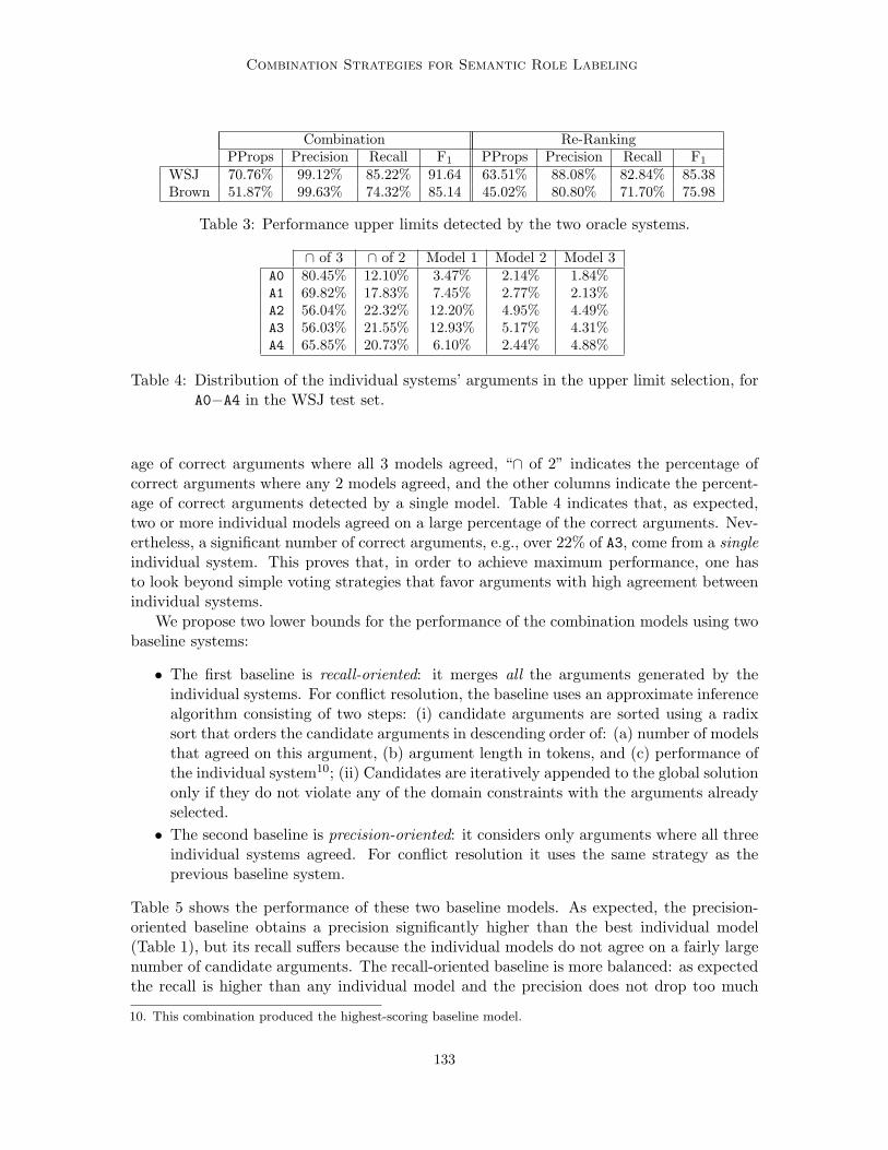
Combination Strategies for Semantic Role Labeling
Combination Re-RankingPProps Precision Recall F1 PProps Precision Recall F1
WSJ 70.76% 99.12% 85.22% 91.64 63.51% 88.08% 82.84% 85.38Brown 51.87% 99.63% 74.32% 85.14 45.02% 80.80% 71.70% 75.98
Table 3: Performance upper limits detected by the two oracle systems.
∩ of 3 ∩ of 2 Model 1 Model 2 Model 3A0 80.45% 12.10% 3.47% 2.14% 1.84%A1 69.82% 17.83% 7.45% 2.77% 2.13%A2 56.04% 22.32% 12.20% 4.95% 4.49%A3 56.03% 21.55% 12.93% 5.17% 4.31%A4 65.85% 20.73% 6.10% 2.44% 4.88%
Table 4: Distribution of the individual systems’ arguments in the upper limit selection, forA0−A4 in the WSJ test set.
age of correct arguments where all 3 models agreed, “∩ of 2” indicates the percentage ofcorrect arguments where any 2 models agreed, and the other columns indicate the percent-age of correct arguments detected by a single model. Table 4 indicates that, as expected,two or more individual models agreed on a large percentage of the correct arguments. Nev-ertheless, a significant number of correct arguments, e.g., over 22% of A3, come from a singleindividual system. This proves that, in order to achieve maximum performance, one hasto look beyond simple voting strategies that favor arguments with high agreement betweenindividual systems.
We propose two lower bounds for the performance of the combination models using twobaseline systems:
• The first baseline is recall-oriented: it merges all the arguments generated by theindividual systems. For conflict resolution, the baseline uses an approximate inferencealgorithm consisting of two steps: (i) candidate arguments are sorted using a radixsort that orders the candidate arguments in descending order of: (a) number of modelsthat agreed on this argument, (b) argument length in tokens, and (c) performance ofthe individual system10; (ii) Candidates are iteratively appended to the global solutiononly if they do not violate any of the domain constraints with the arguments alreadyselected.
• The second baseline is precision-oriented: it considers only arguments where all threeindividual systems agreed. For conflict resolution it uses the same strategy as theprevious baseline system.
Table 5 shows the performance of these two baseline models. As expected, the precision-oriented baseline obtains a precision significantly higher than the best individual model(Table 1), but its recall suffers because the individual models do not agree on a fairly largenumber of candidate arguments. The recall-oriented baseline is more balanced: as expectedthe recall is higher than any individual model and the precision does not drop too much
10. This combination produced the highest-scoring baseline model.
133

Surdeanu, Marquez, Carreras, & Comas
WSJ PProps Prec. Recall F1
baseline recall 53.71% 78.09% 78.77% 78.43 ±0.8
baseline precision 35.43% 92.49% 60.48% 73.14 ±0.9
Brown
baseline recall 36.94% 68.57% 66.05% 67.29 ±2.0
baseline precision 20.52% 88.74% 46.35% 60.89 ±2.1
Table 5: Performance of the baseline models on the WSJ and Brown test sets.
because the inference strategy filters out many unlikely candidates. Overall, the recall-oriented baseline performs best, with an F1 1.22 points higher than the best individualmodel on the WSJ corpus, and 0.41 points lower on the Brown corpus.
8.3 Performance of the Combination System with Constraint Satisfaction
In the Constraint Satisfaction setting the arguments output by individual Models 1, 2, and3 are recombined into an expected better solution that satisfies a set of constraints. Wehave run the inference model based on Constraint Satisfaction described in Section 7.1 usingthe Xpress-MP ILP solver11. The main results are summarized in Table 6. The variantspresented in that table are the following: “Pred-by-pred” stands for local optimization,which processes each verb predicate independently from others, while “Full sentence” standsfor global optimization, i.e., resolving all the verb predicates of the sentence at the sametime. The column labeled “Constraints” shows the particular constraints applied at eachconfiguration. The “O” column presents the value of the parameter for correcting the biastowards candidate overgeneration. Concrete values are empirically set to maximize the F1
measure on the development set. O = 0 corresponds to a setting in which no bias correctionis applied.
Some clear conclusions can be drawn from Table 6. First, we observe that any opti-mization variant obtains F1 results above both the individual systems (Table 1) and thebaseline combination schemes (Table 5). The best combination model scores 2.61 F1 pointsin WSJ and 1.49 in Brown higher than the best individual system. Taking into accountthat no learning is performed, it is clear that Constraint Satisfaction is a simple yet formalsetting that achieves good results.
A somewhat surprising result is that all performance improvements come from con-straints 1 and 2 (i.e., no overlapping nor embedding among arguments of the same verb,and no repetition of core arguments in the same verb). Constraints 3 and 4 are harmful,while the sentence-level constraints (5 and 6) have no impact on the overall performance12.Our analysis of the proposed constraints yielded the following explanations:
• Constraint number 3 prevents the assignment of an R-X argument when the referredargument X is not present. This makes the inference miss some easy R-X arguments
11. Xpress-MP is a Dash Optimization product that is free for academic usage.12. In Section 8.5 we will see that when the learning strategy incorporates global feedback, performing a
sentence-level inference is slightly better than proceeding predicate by predicate.
134

Combination Strategies for Semantic Role Labeling
WSJ Constraints O PProps Precision Recall F1
Pred-by-pred 1 0.30 52.29% 84.20% 75.64% 79.69 ±0.8
1+2 0.30 52.52% 84.61% 75.53% 79.81 ±0.6
1+2+3 0.25 52.31% 84.34% 75.48% 79.67 ±0.7
1+2+4 0.30 51.40% 84.13% 75.04% 79.32 ±0.8
1+2+3+4 0.30 51.19% 83.86% 74.99% 79.18 ±0.7
Full sentence 1+2+5 0.30 52.53% 84.63% 73.53% 79.82 ±0.7
1+2+6 0.30 52.48% 84.64% 75.51% 79.81 ±0.8
1+2+5+6 0.30 52.50% 84.65% 75.51% 79.82 ±0.6
1+2+5+6 0 54.49% 78.74% 79.78% 79.26 ±0.7
Brown
Full sentence 1+2+5+6 0.30 35.70% 78.18% 62.06% 69.19 ±2.1
1+2+5+6 0 38.06% 69.80% 67.85% 68.81 ±2.2
Table 6: Results, on WSJ and Brown test sets, obtained by multiple variants of the con-straint satisfaction approach
when the X argument is not correctly identified (e.g., constituents that start with{that, which, who} followed by a verb are always R-A0). Furthermore, this constraintpresents a lot of exceptions: up to 18.75% of the R-X arguments in the WSJ test set donot have the referred argument X (e.g., “when” in “the law tells them when to do so”),therefore the hard application of constraint 3 prevents the selection of some correctR-X candidates. The official evaluation script from CoNLL-2005 (srl-eval) does notrequire this constraint to be satisfied to consider a solution consistent.
• The srl-eval script requires that constraint number 4 (i.e., a C-X tag is not acceptedwithout a preceding X argument) be fulfilled for a candidate solution to be consideredconsistent. But when it finds a solution violating the constraint its behavior is toconvert the first C-X (without a preceding X) into X. It turns out that this simplepost-processing strategy is better than forcing a coherent solution in the inference stepbecause it allows to recover from the error when an argument has been completelyrecognized but labeled only with C-X tags.
• Regarding sentence-level constraints, we observed that in our setting, inference usinglocal constraints (1+2) rarely produces a solution with inconsistencies at sentencelevel.13 This makes constraint 5 useless since it is almost never violated. Constraintnumber 6 (i.e., no sharing of AMs among different verbs) is more ad-hoc and representsa less universal principle in SRL. The number of exceptions to that constraint, inthe WSJ test set, is 3.0% for the gold-standard data and 4.8% in the output ofthe inference that uses only local constraints (1+2). Forcing the fulfillment of thisconstraint makes the inference process commit as many errors as corrections, makingits effect negligible.
13. This fact is partly explained by the small number of overlapping arguments in the candidate poolproduced by the three individual models.
135

Surdeanu, Marquez, Carreras, & Comas
60
65
70
75
80
85
90
95
-0.4 -0.2 0 0.2 0.4 0.6 0.8 1
%
Value of O
PrecisionRecall
F1
60
65
70
75
80
85
90
95
-0.4 -0.2 0 0.2 0.4 0.6 0.8 1
%
Value of O
PrecisionRecall
F1
Figure 9: Precision-Recall plots, with respect to the bias correcting parameter (O), for theWSJ development and test sets (left and right plots, respectively).
Considering that some of the constraints are not universal, i.e., exceptions exist in thegold standard, it seems reasonable to convert them into soft constraints. This can be doneby precomputing their compatibility from corpora counts using, for instance, point-wisemutual information, and incorporating its effect in the compatibility function as explained insection 7.1. This softening could, in principle, increase the overall recall of the combination.Unfortunately, our initial experiments showed no differences between the hard and softvariants.
Finally, the differences between the optimized values of the bias correcting parameterand O = 0 are clearly explained by observing precision and recall values. The defaultversion tends to overgenerate argument assignments, which implies a higher recall at a costof a lower precision. On the contrary, the F1 optimized variant is more conservative andneeds more evidence to select a candidate. As a result, the precision is higher but the recallis lower. A side effect of being restrictive with argument assignments, is that the numberof correctly annotated complete propositions is also lower in the optimized setting.
The preference for a high-precision vs. a high-recall system is mostly task-dependant.It is interesting to note that in this constraint satisfaction setting, adjusting the precision–recall tradeoff can be easily done by varying the value of the bias correcting score. InFigure 9, we plot the precision–recall curves with respect to different values of the O pa-rameter (the optimization is done using constraints 1, 2, 5, and 6). As expected, high valuesof O promote precision and demote recall, while lower values of O do just the contrary. Also,we see that there is a wide range of values for which the combined F1 measure is almostconstant (the approximate intervals are marked using vertical lines), making it possible toselect different recall and precision values with a global performance (F1) near to the op-timal. Parenthetically, note also that the optimal value estimated on the development set(O = 0.3) generalizes very well to the WSJ test set.
136

Combination Strategies for Semantic Role Labeling
WSJ PProps Prec. Recall F1 F1 improvement
Models 1+2 49.28% 87.39% 72.88% 79.48 ±0.6 +2.27Models 1+3 48.26% 86.80% 73.20% 79.42 ±0.6 +2.96Models 2+3 49.36% 86.63% 73.03% 79.25 ±0.7 +2.04Models 1+2+3 51.66% 87.47% 74.67% 80.56 ±0.6 +3.35
Brown
Models 1+2 34.33% 81.14% 60.86% 69.55 ±2.0 +1.85Models 1+3 31.22% 80.43% 59.07% 68.11 ±1.9 +2.69Models 2+3 32.84% 80.90% 60.31% 69.11 ±2.1 +1.41Models 1+2+3 34.33% 81.75% 61.32% 70.08 ±2.1 +2.38
Table 7: Overall results of the learning-based inference with local rankers on the WSJ andBrown test sets.
8.4 Performance of the Combination System with Local Rankers
We implemented the candidate-scoring classifiers for this combination strategy using Sup-port Vector Machines (SVM) with polynomial kernels of degree 2, which performed slightlybetter than other types of SVMs or AdaBoost. We have implemented the SVM classifierswith the SVMlight software14. Outside of changing the default kernel to polynomial wehave not modified the default parameters. For the experiments reported in this section,we trained models for all 4 possible combinations of our 3 individual systems, using thecomplete feature set introduced in Section 6. The dynamic programming engine used forthe actual inference processes each predicate independently (similar to the “Pred-by-pred”approach in the previous sub-section).
Table 7 summarizes the performance of the combined systems on the WSJ and Browncorpora. Table 7 indicates that our combination strategy is always successful: the resultsof all combination systems improve upon their individual models (Table 1) and their F1
scores are always better than the baselines’ (Table 5). The last column in the table showsthe F1 improvement of the combination model w.r.t. the best individual model in each set.As expected, the highest scoring combined system includes all three individual models. ItsF1 measure is 3.35 points higher than the best individual model (Model 2) in the WSJ testset and 2.38 points higher in the Brown test set. Note that with any combination of twoindividual systems we outperform the current state of the art (see Section 9 for details). Thisis empirical proof that robust and successful combination strategies for the SRL problemare possible. Table 7 also indicates that, even though the partial parsing model (Model 1) isthe worst performing individual model, its contribution to the ensemble is very important,indicating that the information it provides is indeed complementary to the other models’.For instance, in WSJ the performance of the combination of the two best individual models(Models 2+3) is worse than the combinations using model 1 (Models 1+2 and 1+3).
14. http://svmlight.joachims.org/
137

Surdeanu, Marquez, Carreras, & Comas
WSJ PProps Prec. Recall F1
FS1 50.24% 86.47% 73.51% 79.47 ±0.7
+ FS2 50.39% 86.41% 73.68% 79.54 ±0.6
+ FS3 51.22% 86.13% 74.35% 79.80 ±0.7
+ FS4 50.66% 86.67% 74.10% 79.89 ±0.7
+ FS5 51.38% 87.21% 74.61% 80.42 ±0.6
+ FS6 51.66% 87.47% 74.67% 80.56 ±0.6
Brown
FS1 32.21% 80.12% 59.44% 68.25 ±2.0
+ FS2 32.84% 80.80% 59.94% 68.83 ±2.2
+ FS3 33.33% 80.29% 60.82% 69.21 ±2.0
+ FS4 33.33% 81.10% 60.50% 69.30 ±2.1
+ FS5 34.08% 81.76% 61.14% 69.96 ±2.2
+ FS6 34.33% 81.75% 61.32% 70.08 ±1.9
Table 8: Feature analysis for the learning-based inference with local rankers.
Due to its simple architecture −i.e., no feedback from the conflict resolution componentto candidate filtering− this inference model is a good framework to study the contribution ofthe features proposed in Section 6. For this study we group the features into 6 sets: FS1−thevoting features, FS2 −the overlap features with arguments for the same predicate, FS3 −theoverlap features with arguments for other predicates, FS4 −the partial-syntax features, FS5−the full-syntax features, and FS6 −the probabilities generated by the individual systemsfor the candidate arguments. Using these sets we constructed 6 combination models byincreasing the number of features made available to the argument filtering classifiers, e.g.,the first system uses only FS1, the second system adds FS2 to the first system’s features,FS3 is added for the third system, etc. Table 8 lists the performance of these 6 systemsfor the two test corpora. This empirical analysis indicates that the feature sets with thehighest contribution are:
• FS1, which boosts the F1 score of the combined system 2.26 points (WSJ) and 0.55points (Brown) over our best individual system. This is yet another empirical proofthat voting is a successful combination strategy.
• FS5, with a contribution of 0.53 points (WSJ) and 0.66 points (Brown) to the F1
score. These numbers indicate that the filtering classifier is capable of learning someof the “preferences” of the individual models for certain syntactic structures.
• FS3, which contributes 0.26 points (WSJ) and 0.38 points (Brown) to the F1 score.These results promote the idea that information about the overall sentence structure,in our case inter-predicate relations, can be successfully used for the problem of SRL.To our knowledge, this is novel.
All the proposed features have a positive contribution to the performance of the combinedsystem. Overall, we achieve an F1 score that is 1.12 points (WSJ) and 2.33 points (Brown)higher than the best performing combined system at the CoNLL-2005 shared task evaluation(see Section 9 for details).
138

Combination Strategies for Semantic Role Labeling
8.5 Performance of the Combination System with Global Rankers
In this section we report experiments with the global Perceptron algorithm described inSection 7.2.2, that globally trains the scoring functions as rankers. Similar to the localSVM models, we use polynomial kernels of degree 2. Furthermore, the predictions at testtime used averages of the parameter vectors, following the technique of Freund and Schapire(1999).
We were interested in two main aspects. First, we evaluate the effect of training thescoring functions with Perceptron using two different update rules, one global and the otherlocal. The global feedback rule, detailed in Section 7.2.2, corrects the mistakes found whencomparing the correct argument structure with the one that results from the inference (thisis noted as “global” feedback). In contrast, the local feedback rule corrects the mistakesfound before inference, when each candidate argument is handled independently, ignoringthe global argument structure generated (this is noted as “local” feedback). Second, weanalyze the effect of using different constraints in the inference module. To this extent,we configured the inference module in two ways. The first processes the predicates of asentence independently, and thus might select overlapping arguments of different predicates,which is incorrect according to the domain constraints (this one is noted as “Pred-by-pred”inference). The second processes all predicates jointly, and enforces a hierarchical structureof arguments, where arguments never overlap, and arguments of a predicate are allowed toembed arguments of other predicates (this is noted as “Full sentence” inference). From thisperspective, the model with local update and “Pred-by-pred” inference is almost identicalto the local combination strategy described in Section 8.4, with the unique difference thathere we use Perceptron instead of SVM. This apparently minute difference turns out tobe significant for our empirical analysis because it allows us to measure the contributionof both SVM margin maximization and global feedback to the classifier-based combinationstrategy (see Section 8.7).
We trained four different models: with local or global feedback, and with predicate-by-predicate or joint inference. Each model was trained for 5 epochs on the training data,and evaluated on the development data after each training epoch. We selected the bestperforming point on development, and evaluated the models on the test data. Table 9reports the results on test data.
Looking at results, a first impression is that the difference in F1 measure is not verysignificant among different configurations. However, some observations can be pointed out.Global methods achieve much better recall figures, whereas local methods prioritize theprecision of the system. Overall, global methods achieve a more balanced tradeoff betweenprecision and recall, which contributes to a better F1 measure.
Looking at “Pred-by-pred” versus “Full sentence” inference, it can be seen that onlythe global methods are sensitive to the difference. Note that a local model is trainedindependently of the inference module. Thus, adding more constraints to the inferenceengine does not change the parameters of the local model. At testing time, the differentinference configurations do not affect the results. In contrast, the global models are traineddependently of the inference module. When moving from “Pred-by-pred” to “Full sentence”inference, consistency is enforced between argument structures of different predicates, andthis benefits both the precision and recall of the method. The global learning algorithm
139

Surdeanu, Marquez, Carreras, & Comas
WSJ PProps Prec. Recall F1
Pred-by-pred, local 50.71% 86.80% 74.31% 80.07 ±0.7
Full sentence, local 50.67% 86.80% 74.29% 80.06 ±0.7
Pred-by-pred, global 53.45% 84.66% 76.19% 80.20 ±0.7
Full sentence, global 53.81% 84.84% 76.30% 80.34 ±0.6
Brown
Pred-by-pred, local 33.33% 80.62% 60.77% 69.30 ±1.9
Full sentence, local 33.33% 80.67% 60.77% 69.32 ±2.0
Pred-by-pred, global 35.20% 77.65% 62.70% 69.38 ±1.9
Full sentence, global 35.95% 77.91% 63.02% 69.68 ±2.0
Table 9: Test results of the combination system with global rankers. Four configurations areevaluated, that combine “Pred-by-pred” or “Full sentence” inference with “local”or “global” feedback.
improves both in precision and recall when coupled with a joint inference process thatconsiders more constraints in the solution.
Nevertheless, the combination system with local SVM classifiers, presented in the previ-ous section, achieves marginally better F1 score than the global learning method (80.56% vs.80.34% in WSJ). This is explained by the different machine learning algorithms (we discussthis issue in detail in Section 8.7). The better F1 score is accomplished by a much betterprecision in the local approach (87.47% vs. 84.84% in WSJ), whereas the recall is lower inthe local than in the global approach (74.67% vs. 76.30% in WSJ). On the other hand, theglobal strategy produces more completely-correct annotations (see the “PProps” column)than any of the local strategies investigated (see Tables 9 and 7). This is to be expected,considering that the global strategy optimizes a sentence-level cost function. Somewhatsurprisingly, the number of perfect propositions generated by the global strategy is lowerthan the number of perfect propositions produced by the constraint-satisfaction approach.We discuss this result in Section 8.7.
8.6 Scalability of the Combination Strategies
All the combination experiments reported up to this point used the candidate argumentsgenerated by the three individual SRL models introduced in Section 4. While these experi-ments do provide an empirical comparison of the three inference models proposed, they donot answer an obvious scalability question: how do the proposed combination approachesscale when the number of candidate arguments increases but their quality diminishes? Weare mainly interested in answering this question for the last two combination models (whichuse inference based on learning with local or global rankers) for two reasons: (a) theyperformed better than the constraint satisfaction model in our previous experiments, and(b) because they have no requirements on the individual SRL systems’ outputs −unlikethe constraint satisfaction model which requires the argument probabilities of the individ-ual models− they can be coupled to pools of candidates generated by any individual SRLmodel.
140

Combination Strategies for Semantic Role Labeling
WSJ BrownPProps Prec. Recall F1 PProps Prec. Recall F1
koomen√
53.79% 82.28% 76.78% 79.44 32.34% 73.38% 62.93% 67.75pradhan+
√52.61% 82.95% 74.75% 78.63 38.93% 74.49% 63.30% 68.44
haghighi√
56.52% 79.54% 77.39% 78.45 37.06% 70.24% 65.37% 67.71marquez
√51.85% 79.55% 76.45% 77.97 36.44% 70.79% 64.35% 67.42
pradhan × 50.14% 81.97% 73.27% 77.37 36.44% 73.73% 61.51% 67.07
surdeanu√
45.28% 80.32% 72.95% 76.46 29.48% 72.41% 59.67% 65.42tsai
√45.43% 82.77% 70.90% 76.38 30.47% 73.21% 59.49% 65.64
che√
47.81% 80.48% 72.79% 76.44 31.84% 71.13% 59.99% 65.09moschitti
√47.66% 76.55% 75.24% 75.89 30.85% 65.92% 61.83% 63.81
tjongkimsang√
45.85% 79.03% 72.03% 75.37 28.36% 70.45% 60.13% 64.88yi × 47.50% 77.51% 72.97% 75.17 31.09% 67.88% 59.03% 63.14
ozgencil√
46.19% 74.66% 74.21% 74.44 31.47% 65.52% 62.93% 64.20
Table 10: Performance of the best systems at CoNLL-2005. The “pradhan+” contains post-evaluation improvements. The top 5 systems are actually combination modelsthemselves. The second column marks with × the systems not used in our evalu-ation: “pradhan”, which was replaced by its improved version “pradhan+”, and“yi”, due to format errors in the submitted data.
For this scalability analysis, we use as individual SRL models the top 10 systems at theCoNLL-2005 shared task evaluation. Table 10 summarizes the performance of these systemson the same two test corpora used in our previous experiments. As Table 10 indicates, theperformance of these systems varies widely: there is a difference of 5 F1 points in the WSJcorpus and of over 4 F1 points in the Brown corpus between the best and the worst systemin this set.
For the combination experiments we generated 5 candidate pools using the top 2, 4, 6,8, and 10 individual systems labeled with
√in Table 10. We had to make two changes
to the experimental setup used in the first part of this section: (a) we trained our com-bined models on the PropBank development section because we did not have access to theindividual systems’ outputs on the PropBank training partition; and (b) from the featureset introduced in Section 6 we did not use the individual systems’ argument probabilitiesbecause the raw activations of the individual models’ classifiers were not available. Notethat under these settings the size of the training corpus is 10 times smaller than the size ofthe training set used in the previous experiments.
Table 11 shows the upper limits of these setups using the “combination” and “re-ranking” oracle systems introduced in Section 8.2. Besides performance numbers, we alsolist in Table 11 the average number of candidates per sentence for each setup, i.e., numberof unique candidate arguments (“# Args./Sent.”) for the “combination” oracle and numberof unique candidate frames (“# Frames/Sent.”) for the “re-ranking” oracle. Table 12 liststhe performance of our combined models with both local feedback (Section 7.2.1) and globalfeedback (Section 7.2.2). The combination strategy with global rankers uses joint inferenceand global feedback (see the description in the previous sub-section).
141

Surdeanu, Marquez, Carreras, & Comas
Combination Re-RankingWSJ # Args./Sent. Prec. Recall F1 # Frames/Sent. Prec. Recall F1
C2 8.53 99.34% 82.71% 90.27 3.16 88.63% 81.77% 85.07C4 9.78 99.47% 87.26% 92.96 4.44 91.08% 86.12% 88.53C6 10.23 99.47% 88.02% 93.39 7.21 92.14% 86.57% 89.27C8 10.74 99.48% 88.63% 93.75 8.11 92.88% 87.33% 90.02
C10 11.33 99.50% 89.02% 93.97 8.97 93.31% 87.71% 90.42Brown
C2 7.42 99.62% 71.34% 83.14 3.02 82.45% 70.37% 75.94C4 8.99 99.65% 77.58% 87.24 4.55 86.01% 75.98% 80.68C6 9.62 99.65% 79.38% 88.37 7.09 88.19% 76.80% 82.10C8 10.24 99.66% 80.52% 89.08 8.19 88.95% 78.04% 83.14
C10 10.86 99.66% 81.72% 89.80 9.21 89.65% 79.19% 84.10
Table 11: Performance upper limits determined by the oracle systems on the 10 best sys-tems at CoNLL-2005. Ck stands for combination of the top k systems fromTable 10. “# Args./Sent.” indicates the average number of candidate argumentsper sentence for the combination oracle; “# Frames/Sent.” indicates the averagenumber of candidate frames per sentence for the re-ranking oracle. The lattercan be larger than the number of systems in the combination because on averagethere are multiple predicates per sentence.
Local ranker Global rankerWSJ PProps Prec. Recall F1 PProps Prec. Recall F1
C2 50.69% 86.60% 73.90% 79.75±0.7 52.74 84.07% 75.38% 79.49±0.7
C4 55.14% 86.67% 76.63% 81.38±0.7 54.95 84.00% 77.19% 80.45±0.7
C6 54.85% 87.45% 76.34% 81.52±0.6 55.21 84.24% 77.41% 80.68±0.7
C8 54.36% 87.49% 76.12% 81.41±0.6 55.00 84.42% 77.10% 80.59±0.7
C10 53.90% 87.48% 75.81% 81.23±0.6 54.76 84.02% 77.44% 80.60±0.7
BrownC2 32.71% 79.56% 60.45% 68.70±1.8 35.32 74.88% 62.43% 68.09±2.0
C4 35.95% 80.27% 63.16% 70.69±2.0 39.30 75.63% 64.45% 69.59±2.2
C6 35.32% 80.94% 62.24% 70.37±1.8 37.44 76.12% 64.58% 69.88±2.0
C8 35.95% 81.98% 61.87% 70.52±2.2 38.43 76.40% 64.08% 69.70±2.2
C10 36.32% 82.61% 61.97% 70.81±2.0 37.44 75.94% 64.68% 69.86±2.0
Table 12: Local versus global ranking for combinations of the 10 best systems at CoNLL-2005. Ck stands for combination of the top k systems from Table 10.
We can draw several conclusions from these experiments. First, the performance up-per limit of re-ranking is always lower than that that of the argument-based combinationstrategy, even when the number of candidates is large. For example, when all 10 individualmodels are used, the F1 upper limit of our approach in the Brown corpus is 89.80 whereasthe F1 upper limit for re-ranking is 84.10. However, the enhanced potential of our combina-tion approach does not imply a significant increase in computational cost: Table 11 shows
142

Combination Strategies for Semantic Role Labeling
that the number of candidate arguments that must be handled by combination approachesis not that much higher than the number of candidate frames input to the re-ranking sys-tem, especially when the number of individual models is high. For example, when all 10individual models are used, the combination approaches must process around 11 argumentsper sentence, whereas re-ranking approaches must handle approximately 9 frames per sen-tence. The intuition behind this relatively small difference in computational cost is that,even though the number of arguments is significantly larger than the number of frames,the difference between the number of unique candidates for the two approaches is not highbecause the probability of repeated arguments is higher than the probability of repeatedframes.
The second conclusion is that all our combination models boost the performance of thecorresponding individual systems. For example, the best 4-system combination achieves anF1 score approximately 2 points higher than the best individual model in both the WSJand Brown corpus. As expected, the combination models reach a performance plateauaround 4-6 individual systems, when the quality of the individual models starts to dropsignificantly. Nevertheless, considering that the top 4 individual systems use combinationstrategies themselves and the amount of training data for this experiment was quite small,these results show the good potential of the combination models analyzed in this paper.
The third observation is that the relation previously observed between local and globalrankers holds: our combination model with local rankers has better precision, but the modelwith global rankers always has better recall and generally better PProps score. Overall,the model with local rankers obtains better F1 scores and scales better as the numberof individual systems increases. We discuss these differences in more detail in the nextsub-section.
Finally, Table 11 indicates that the potential recall of this experiment (shown in theleft-most block in the table) is higher than the potential recall when combining our threeindividual SRL systems (see Table 3): 3.8% higher in the WSJ test set, and 7.4% higher inthe Brown test set. This was expected, considering that both the number and the qualityof the candidate arguments in this last experiment is higher. However, even after thisimprovement, the potential recall of our combination strategies is far from 100%. Thus,combining the solutions of the N best state-of-the-art SRL systems still does not havethe potential to properly solve the SRL problem. Future work should focus on recall-boosting strategies, e.g., using candidate arguments of the individual systems before theindividual complete solutions are generated, because in this step many candidate argumentsare eliminated.
8.7 Discussion
The experimental results presented in this section indicate that all proposed combinationstrategies are successful: all three combination models provide statistically significant im-provements over the individual models and the baselines in all setups. An immediate (butsomewhat shallow) comparison of the three combination strategies investigated indicatesthat: (a) the best combination strategy for the SRL problem is a max-margin local meta-learner; (b) the global ranking approach for the meta-learner is important but it does not
143

Surdeanu, Marquez, Carreras, & Comas
have the same contribution as a max-margin strategy; and (c) the constraint-satisfactionmodel performs the worst of all the strategies tried.
However, in most experiments the differences between the combination approaches in-vestigated are small. A more reasonable observation is that each combination strategy hasits own advantages and disadvantages and different approaches are suitable for differentapplications and data. We discuss these differences below.
If the argument probabilities of individual systems are available, the combination modelbased on constraint satisfaction is an attractive choice: it is a simple, unsupervised strat-egy that obtains competitive performance. Furthermore, the constraint satisfaction modelprovides an elegant and customizable framework to tune the balance between precision andrecall (see Section 8.3). With this framework we currently obtain the highest recall of allcombination models: 3.48% higher than the best recall obtained by the meta-learning ap-proaches on the WSJ corpus, and 4.83% higher than the meta-learning models on the Browncorpus. The higher recall implies also higher percentage of predicates that are completelycorrectly annotated: the best “PProps” numbers in Table 6 are the best of all combinationstrategies. The cause for this high difference in recall in favor of the constraint satisfactionapproach is that the candidate scoring of the learning-based inference acts implicitly as afilter: all candidates whose score −i.e., the classifier confidence that the candidate is part ofthe correct solution− is negative are discarded, which negatively affects the overall recall.Hence, constraint satisfaction is a better solution for SRL-based NLP applications whichrequire that predicate-argument frames be extracted with high recall. For example, in Infor-mation Extraction, predicate-argument tuples are filtered with subsequent high-precision,domain-specific constraints (Surdeanu et al., 2003), hence it is paramount that the SRLmodel have high recall.
Nevertheless, in many cases the argument probabilities of the individual SRL models arenot available, either because the models do not generate them, e.g., rule-based systems, orbecause the individual models are available only as black boxes, which do not offer access tointernal information. Under these conditions, we showed that combination strategies basedon meta-learning are a viable alternative. In fact, these approaches obtain the highestF1 scores (see Section 8.4) and obtain excellent performance even with small amounts oftraining data (see Section 8.6). As previously mentioned, because candidate scoring actsas filter, the learning-based inference tends to favor precision over recall: their precisionis 2.82% higher than the best precision of the constraint-satisfaction models in the WSJcorpus, and 3.57% higher in the Brown corpus. This preference for precision over recall ismore pronounced in the learning-based inference with local rankers (Section 8.4) than inthe inference model with global rankers (Section 8.5). Our hypothesis for what causes theglobal-ranking model to be less precision-biased is that in this configuration the ratio oferrors on positive versus negative samples is more balanced. Thinking in the strategy thatPerceptron follows, a local approach updates at every candidate with incorrect predictionsign, whereas a global approach only updates at candidates that should or should not be inthe complete solution, after enforcing the domain constraints. In other words, the numberof negative updates −which drives the precision bias− is reduced in the global approach,because some of the false positives generated by the ranking classifiers are eliminated bythe domain constraints. Thus, because candidate scoring is trained to optimize accuracy,
144

Combination Strategies for Semantic Role Labeling
WSJ PProps Prec. Recall F1
global feedback +3.10% -1.96% +1.99% +0.27max margin +0.95% +0.67% +0.36% +0.49
Brown
global feedback +2.62% -2.71% +2.25% +0.38max margin +1.00% +1.13% +0.55% +0.78
Table 13: Contribution of global feedback and max margin to the learning-based inference.The baseline is the “Pred-by-pred, local” model in Table 9.
fewer candidate arguments will be eliminated by the meta-learner with global rankers, whichtranslates into a better balance between precision and recall.
Another important conclusion of our analysis of global versus local ranking for thelearning-based inference is that a max-margin approach for the candidate scoring classifiersis more important than having global feedback for inference. In fact, considering that theonly difference between the model with predicate-by-predicate inference with local feedbackin Section 8.5 (“Pred-by-pred, local”) versus the best model in Section 8.4 (+FS6) is that thelatter uses SVM classifiers whereas the former uses Perceptron, we can compute the exactcontribution of both max margin and global feedback15. For convenience, we summarize thisanalysis in Table 13. That table indicates that max margin yields a consistent improvementof both precision and recall, whereas the contribution of global feedback is more in reducingthe difference between precision and recall by boosting recall and decreasing precision. Thebenefit of max-margin classifiers is even more evident in Table 12, which shows that thelocal-ranking model with max-margin classifiers generalizes better than the global-rankingmodel when the amount of training data is reduced significantly.
Even though in this paper we have analyzed several combination approaches with threeindependent implementations, the proposed models are in fact compatible with each other.Various combinations of the proposed strategies are immediately possible. For example, theconstraint satisfaction model can be applied on the output probabilities of the candidatescoring component introduced in Section 7.2. Such a model eliminates the dependencyon the output scores of the individual SRL models but retains all the advantages of theconstraint satisfaction model, e.g., the formal framework to tune the balance between pre-cision and recall. Another possible combination of the approaches introduced in this paperis to use max-margin classifiers in the learning-based inference with global feedback, e.g.,by using a global training method for margin maximization such as SVMstruct (Tsochan-taridis et al., 2004). This model would indeed have an increased training time16, but couldleverage the advantages of both max-margin classifiers and inference with global feedback(summarized in Table 13). Finally, another attractive approach is stacking, i.e., N lev-els of chained meta-learning. For example, we could cascade the learning-based inferencemodel with global rankers, which boosts recall, with the learning-based inference with localrankers, which favors precision.
15. The contribution of global feedback is given by the model with joint inference and global feedback (“Fullsentence, global”) in Section 8.5.
16. This was the main reason why we chose Perceptron for the proposed online strategies.
145

Surdeanu, Marquez, Carreras, & Comas
9. Related Work
The 4 best performing systems at the CoNLL-2005 shared task included a combination ofdifferent base subsystems to increase robustness and to gain coverage and independencefrom parse errors. Therefore, they are closely related to the work of this paper. The firstfour rows in Table 10 summarize their results under exactly the same experimental settingas the one used in this paper.
Koomen et al. (2005) used a 2 layer architecture close to ours. The pool of candidates isgenerated by: (a) running a full syntax SRL system on alternative input information (Collinsparsing, and 5-best trees from Charniak’s parser), and (b): taking all candidates that passa filter from the set of different parse trees. The combination of candidates is performedin an elegant global inference procedure as constraint satisfaction, which, formulated asInteger Linear Programming, is solved efficiently. This is different from our work, wherewe “break” complete solutions from any number of SRL systems and we also investigatea meta-learning combination approach in addition to the ILP inference. Koomen et al.’ssystem was the best performing system at CoNLL-2005 (see Table 10).
Haghighi et al. (2005) implemented double re-ranking on top of several outputs from abase SRL model. The re-ranking is performed, first, on a set of n-best solutions obtainedby the base system run on a single parse tree, and, then, on the set of best-candidatescoming from the n-best parse trees. This was the second-best system at CoNLL-2005(third row in Table 10). Compared to our decomposition and re-combination approach,the re-ranking setting has the advantage of allowing the definition of global features thatapply to complete candidate solutions. According to a follow-up work by the same authors(Toutanova, Haghighi, & Manning, 2005), these global features are the source of the majorperformance improvements of the re-ranking system. In contrast, we focus more on featuresthat exploit the redundancy between the individual models, e.g., overlap between individualcandidate arguments, and we add global information at frame level only from the completesolutions provided by individual models. The main drawback of re-ranking compared to ourapproach is that the different individual solutions can not be combined because re-rankingis forced to select a complete candidate solution. This implies that its overall performancestrongly depends on the ability of the base model to generate the complete correct solutionin the set of n-best candidates. This drawback is evident in the lower performance upperlimit of the re-ranking approach (see Tables 3 and 11) and in the performance of the actualsystem —our best combination strategy achieves an F1 score over 2 points higher thanHaghighi et al. in both WSJ and Brown17.
Finally, Pradhan, Hacioglu, Ward, Martin, and Jurafsky (2005b) followed a stackingapproach by learning two individual systems based on full syntax, whose outputs are used togenerate features to feed the training stage of a final chunk-by-chunk SRL system. Althoughthe fine granularity of the chunking-based system allows to recover from parsing errors, wefind this combination scheme quite ad-hoc because it forces to break argument candidatesinto chunks in the last stage.
17. Recently, Yih and Toutanova (2006) reported improved numbers for this system: 80.32 F1 for WSJ and68.81 for Brown. However, these numbers are not directly comparable with the systems presented inthis paper because they fixed a significant bug in the representation of quotes in the input data, a bugthat is still present in our data.
146

Combination Strategies for Semantic Role Labeling
Outside of the CoNLL shared task evaluation, Roth and Yih (2005) reached the con-clusion that the quality of the local argument classifiers is more important than the globalfeedback from the inference component. This is also one of the conclusions drawn by this pa-per. Our contribution is that we have shown that this hypothesis holds in a more complexframework: combination of several state-of-the-art individual models, whereas Roth andYih experimented with a single individual model, only numbered arguments, and a slightlysimplified problem representation: B-I-O over basic chunks. Additionally, our more detailedexperiments allowed us to show clearly that the contribution of max margin is higher thanthat of global learning in several corpora and for several combinations of individual systems.
Punyakanok, Roth, and Yih (2005) showed that the performance of individual SRLmodels (particularly argument identification) is significantly improved when full parsing isused and argument boundaries are restricted to match syntactic constituents (similarly toour Model 3). We believe that the approach used by our Models 1 and 2, where candidatearguments do not have to match a single syntactic constituent, has increased robustnessbecause it has a built-in mechanism to handle some syntax errors, when an argument con-stituent is incorrectly fragmented into multiple phrases. Our empirical results support thisclaim: Model 2 performs better than both Model 3 and the models proposed by Punyakanoket al. A second advantage of the strategy proposed in this paper is that the same modelcan be deployed using full syntax (Model 2) or partial syntax (Model 1).
Pradhan, Ward, Hacioglu, Martin, and Jurafsky (2005c) implement a SRL combinationstrategy at constituent level that, similarly to our approach, combines different syntacticviews of the data based on full and partial syntactic analysis. However, unlike our approach,Pradhan et al.’s work uses only a simple greedy inference strategy based on the probabilitiesof the candidate arguments, whereas in this paper we introduce and analyze three differentcombination algorithms. Our analysis yielded a combination system that outperforms thecurrent state of the art.
Previous work in the more general field of predicting structures in natural languagetexts has indicated that the combination of several individual models improves overall per-formance in the given task. Collins (2000) first proposed a learning layer based on rankingto improve the performance of a generative syntactic parser. In that approach, a rerankerwas trained to select the best solution from a pool of solutions produced by the generativeparser. In doing so, the reranker dealt with complete parse trees, and represented them withrich features that exploited dependencies not considered in the generative method. On theother hand, it was computationally feasible to train the reranker, because the base methodreduced the number of possible parse trees for a sentence from an exponential number (w.r.t.sentence length) to a few tens. More recently, global discriminative learning methods forpredicting structures have been proposed (Lafferty, McCallum, & Pereira, 2001; Collins,2002, 2004; Taskar et al., 2003, 2004; Tsochantaridis et al., 2004). All of them train asingle discriminative ranking function to detect structures in a sentence. A major propertyof these methods is that they model the problem discriminatively, so that arbitrary andrich representations of structures can be used. Furthermore, the training process in thesemethods is global, in that parameters are set to maximize measures not only related tolocal accuracies (i.e., on recognizing parts of a structure), but also related to the globalaccuracy (i.e., on recognizing complete structures). In this article, the use of global andrich representations is also a major motivation.
147

Surdeanu, Marquez, Carreras, & Comas
10. Conclusions
This paper introduces and analyzes three combination strategies in the context of semanticrole labeling: the first model implements an inference strategy with constraint satisfactionusing integer linear programming, the second uses inference based on learning where thecandidates are scored using discriminative classifiers using only local information, and thethird and last inference model builds on the previous strategy by adding global feedbackfrom the conflict resolution component to the ranking classifiers. The meta-learners usedby the inference process are developed with a rich set of features that includes votingstatistics −i.e., how many individual systems proposed a candidate argument− overlapwith arguments from the same and other predicates in the sentence, structure and distanceinformation coded using partial and full syntax, and probabilities from the individual SRLmodels (if available). To our knowledge, this is the first work that: (a) introduces a thoroughinference model based on learning for semantic role labeling, and (b) performs a comparativeanalysis of several inference strategies in the context of SRL.
The results presented suggest that the strategy of decomposing individual solutions andperforming a learning-based re-combination for constructing the final solution has advan-tages over other approaches, e.g., re-ranking a set of complete candidate solutions. Ofcourse, this is a task-dependant conclusion. In the case of semantic role labeling, our ap-proach is relatively simple since the re-combination of argument candidates has to fulfillonly a few set of structural constraints to generate a consistent solution. If the target struc-ture is more complex (e.g., a full parse tree) the re-combination step might be too complexfrom both the learning and search perspectives.
Our evaluation indicates that all proposed combination approaches are successful: theyall provide significant improvements over the best individual model and several baselinecombination algorithms in all setups. Out of the three combination strategies investigated,the best F1 score is obtained by the learning-based inference using max-margin classifiers.While all the proposed approaches have their own advantages and drawbacks (see Section 8.7for a detailed discussion of differences among the proposed inference models) several im-portant features of a state-of-the-art SRL combination strategy emerge from this analysis:(i) individual models should be combined at the granularity of candidate arguments ratherthan at the granularity of complete solutions or frames; (ii) the best combination strategyuses an inference model based in learning; (iii) the learning-based inference benefits frommax-margin classifiers and global feedback, and (iv) the inference at sentence level (i.e.,considering all predicates at the same time) proves only slightly useful when the learning isperformed also globally, using feedback from the complete solution after inference.
Last but not least, the results obtained with the best combination strategy developedin this work outperform the current state of the art. These results are empirical proof thata SRL system with good performance can be built by combining a small number (three inour experiments) of relatively simple SRL models.
Acknowledgments
We would like to thank the JAIR reviewers for their valuable comments.This research has been partially supported by the European Commission (CHIL project,
148

Combination Strategies for Semantic Role Labeling
IP-506909; PASCAL Network, IST-2002-506778) and the Spanish Ministry of Educationand Science (TRANGRAM, TIN2004-07925-C03-02). Mihai Surdeanu is a research fellowwithin the Ramon y Cajal program of the Spanish Ministry of Education and Science. Weare also grateful to Dash Optimization for the free academic use of Xpress-MP.
References
Bishop, C. (1995). Neural Networks for Pattern Recognition. Oxford University Press.
Boas, H. C. (2002). Bilingual framenet dictionaries for machine translation. In Proceedingsof LREC 2002.
Carreras, X., & Marquez, L. (2004). Introduction to the CoNLL-2004 shared task: Semanticrole labeling. In Proceedings of CoNLL 2004.
Carreras, X., & Marquez, L. (2005). Introduction to the conll-2005 shared task: Semanticrole labeling. In Proceedings of CoNLL-2005.
Carreras, X., Marquez, L., & Chrupa�la, G. (2004). Hierarchical recognition of propositionalarguments with perceptrons. In Proceedings of CoNLL 2004 Shared Task.
Charniak, E. (2000). A maximum-entropy-inspired parser. In Proceedings of NAACL.
Collins, M. (1999). Head-Driven Statistical Models for Natural Language Parsing. PhDDissertation, University of Pennsylvania.
Collins, M. (2000). Discriminative reranking for natural language parsing. In Proceedingsof the 17th International Conference on Machine Learning, ICML-00, Stanford, CAUSA.
Collins, M. (2002). Discriminative training methods for hidden markov models: Theory andexperiments with perceptron algorithms. In Proceedings of the SIGDAT Conferenceon Empirical Methods in Natural Language Processing, EMNLP-02.
Collins, M. (2004). Parameter estimation for statistical parsing models: Theory and prac-tice of distribution-free methods. In Bunt, H., Carroll, J., & Satta, G. (Eds.), NewDevelopments in Parsing Technology, chap. 2. Kluwer.
Collins, M., & Duffy, N. (2002). New ranking algorithms for parsing and tagging: Kernelsover discrete structures, and the voted perceptron. In Proceedings of the 40th AnnualMeeting of the Association for Computational Linguistics, ACL’02.
Crammer, K., & Singer, Y. (2003a). A family of additive online algorithms for categoryranking. Journal of Machine Learning Research, 3, 1025–1058.
Crammer, K., & Singer, Y. (2003b). Ultraconservative online algorithms for multiclassproblems. Journal of Machine Learning Research, 3, 951–991.
Freund, Y., & Schapire, R. E. (1999). Large margin classification using the perceptronalgorithm. Machine Learning, 37 (3), 277–296.
Gildea, D., & Jurafsky, D. (2002). Automatic labeling of semantic roles. ComputationalLinguistics, 28 (3).
149

Surdeanu, Marquez, Carreras, & Comas
Gildea, D., & Palmer, M. (2002). The necessity of syntactic parsing for predicate argumentrecognition. In Proceedings of the 40th Annual Conference of the Association forComputational Linguistics (ACL-02).
Hacioglu, K., Pradhan, S., Ward, W., Martin, J. H., & Jurafsky, D. (2004). Semanticrole labeling by tagging syntactic chunks. In Proceedings of the 8th Conference onComputational Natural Language Learning (CoNLL-2004).
Haghighi, A., Toutanova, K., & Manning, C. (2005). A joint model for semantic role labeling.In Proceedings of CoNLL-2005 Shared Task.
Koomen, P., Punyakanok, V., Roth, D., & Yih, W. (2005). Generalized inference withmultiple semantic role labeling systems. In Proceedings of CoNLL-2005 Shared Task.
Lafferty, J., McCallum, A., & Pereira, F. (2001). Conditonal random fields: Probabilis-tic models for segmenting and labeling sequence data. In Proceedings of the 18thInternational Conference on Machine Learning, ICML-01.
Marcus, M., Santorini, B., & Marcinkiewicz, M. (1994). Building a large annotated corpusof English: The Penn Treebank. Computational Linguistics, 19 (2).
Marquez, L., Comas, P., Gimenez, J., & Catala, N. (2005). Semantic role labeling assequential tagging. In Proceedings of CoNLL-2005 Shared Task.
Melli, G., Wang, Y., Liu, Y., Kashani, M. M., Shi, Z., Gu, B., Sarkar, A., & Popowich,F. (2005). Description of SQUASH, the SFU question answering summary handlerfor the DUC-2005 summarization task. In Proceedings of Document UnderstandingWorkshop, HLT/EMNLP Annual Meeting.
Narayanan, S., & Harabagiu, S. (2004). Question answering based on semantic structures.In International Conference on Computational Linguistics (COLING 2004).
Noreen, E. W. (1989). Computer-Intensive Methods for Testing Hypotheses. John Wiley &Sons.
Palmer, M., Gildea, D., & Kingsbury, P. (2005). The Proposition Bank: An annotatedcorpus of semantic roles. Computational Linguistics, 31 (1).
Ponzetto, S. P., & Strube, M. (2006a). Exploiting semantic role labeling, wordnet andwikipedia for coreference resolution. In Proceedings of the Human Language TechnolgyConference of the North American Chapter of the Association for Computational Lin-guistics.
Ponzetto, S. P., & Strube, M. (2006b). Semantic role labeling for coreference resolution. InCompanion Volume of the Proceedings of the 11th Meeting of the European Chapterof the Association for Computational Linguistics.
Pradhan, S., Hacioglu, K., Krugler, V., Ward, W., Martin, J. H., & Jurafsky, D. (2005a).Support vector learning for semantic argument classification. Machine Learning, 60,11–39.
Pradhan, S., Hacioglu, K., Ward, W., Martin, J. H., & Jurafsky, D. (2005b). Semantic rolechunking combining complementary syntactic views. In Proceedings of CoNLL-2005.
150

Combination Strategies for Semantic Role Labeling
Pradhan, S., Ward, W., Hacioglu, K., Martin, J. H., & Jurafsky, D. (2005c). Semantic rolelabeling using different syntactic views. In Proceedings of the 43rd Annual Conferenceof the Association for Computational Linguistics.
Punyakanok, V., Roth, D., & Yih, W. (2005). The necessity of syntactic parsing for seman-tic role labeling. In Proceedings of the International Joint Conference on ArtificialIntelligence (IJCAI).
Punyakanok, V., Roth, D., Yih, W., & Zimak, D. (2004). Semantic role labeling via inte-ger linear programming inference. In Proceedings of the International Conference onComputational Linguistics (COLING’04).
Rosenblatt, F. (1958). The perceptron: A probabilistic model for information storage andorganization in the brain. Psychological Review, 65, 386–407.
Roth, D., & Yih, W. (2004). A linear programming formulation for global inference innatural language tasks. In Proceedings of the Annual Conference on ComputationalNatural Language Learning (CoNLL-2004), pp. 1–8, Boston, MA.
Roth, D., & Yih, W. (2005). Integer linear programming inference for conditional randomfields. In Proceedings of the International Conference on Machine Learning (ICML).
Schapire, R. E., & Singer, Y. (1999). Improved boosting algorithms using confidence-ratedpredictions. Machine Learning, 37 (3).
Surdeanu, M., Harabagiu, S., Williams, J., & Aarseth, P. (2003). Using predicate-argumentstructures for information extraction. In Proceedings of the 41st Annual Meeting ofthe Association for Computational Linguistics (ACL 2003).
Taskar, B., Guestrin, C., & Koller, D. (2003). Max-Margin Markov Networks. In Proceedingsof the 17th Annual Conference on Neural Information Processing Systems, NIPS-03,Vancouver, Canada.
Taskar, B., Klein, D., Collins, M., Koller, D., & Manning, C. (2004). Max-margin parsing.In Proceedings of the EMNLP-2004.
Toutanova, K., Haghighi, A., & Manning, C. (2005). Joint learning improves semantic rolelabeling. In Proceedings of the 43rd Annual Meeting of the Association for Compu-tational Linguistics (ACL’05), pp. 589–596, Ann Arbor, MI, USA. Association forComputational Linguistics.
Tsochantaridis, I., Hofmann, T., Joachims, T., & Altun, Y. (2004). Support vector machinelearning for interdependent and structured output spaces. In Proceedings of the 21stInternational Conference on Machine Learning, ICML-04.
Xue, N., & Palmer, M. (2004). Calibrating features for semantic role labeling. In Proceedingsof EMNLP-2004.
Yih, S. W., & Toutanova, K. (2006). Automatic semantic role labeling. In Tutorial ofthe Human Language Technolgy Conference of the North American Chapter of theAssociation for Computational Linguistics.
Younger, D. H. (1967). Recognition and parsing of context-free languages in n3 time.Information and Control, 10 (2), 189–208.
151