colpack: software for graph coloring and related problems...

A

ColPack: Software for Graph Coloring and Related Problems inScientific Computing

ASSEFAW H. GEBREMEDHIN, Purdue University

DUC NGUYEN, Purdue University

MD. MOSTOFA ALI PATWARY, Northwestern University

ALEX POTHEN, Purdue University

We present a suite of fast and effective algorithms, encapsulated in a software package called ColPack, for

a variety of graph coloring and related problems. Many of the coloring problems model partitioning needs

arising in compression-based computation of Jacobian and Hessian matrices using Algorithmic Differenti-ation. Several of the coloring problems also find important applications in many areas outside derivative

computation, including frequency assignment in wireless networks, scheduling, facility location, and con-currency discovery and data movement operations in parallel and distributed computing. The presentation

in this article includes a high-level description of the various coloring algorithms within a common design

framework, a detailed treatment of the theory and efficient implementation of known as well as new vertexordering techniques upon which the coloring algorithms rely, a discussion of the package’s software design,

and an illustration of its usage. The article also includes an extensive experimental study of the major

algorithms in the package using real-world as well as synthetically generated graphs.

Categories and Subject Descriptors: F.2.1 [Numerical Algorithms and Problems]: Computations on

matrices; F.2.2 [Nonnumerical Algorithms and Problems]: Computations on discrete structures; G.1.6

[Optimization]: Nonlinear programming; G.2.2 [Graph Theory]: Graph algorithms; G.4 [MathematicalSoftware]: Algorithm design and analysis

General Terms: Algorithms, Design, Experimentation, Performance

Additional Key Words and Phrases: Automatic Differentiation, Combinatorial optimization, Graph color-ing, Greedy coloring algorithms, Nonlinear optimization, Sparse derivative computation, Vertex ordering

techniques

ACM Reference Format:Gebremedhin, A.H., Nguyen, D., Patwary, M.M.A., and Pothen, A. 2013. ColPack: Software for Graph

Coloring and Related Problems in Scientific Computing. ACM Trans. Math. Softw. V, N, Article A (January

YYYY), 30 pages.DOI = 10.1145/0000000.0000000 http://doi.acm.org/10.1145/0000000.0000000

1. INTRODUCTION AND OVERVIEW

In many mathematical or computational contexts, one encounters the need for partitioninga set of binary-related objects into as few subsets of independent objects as possible so thatsome “scarce” resource is optimally used. Graph coloring in a generic sense is an abstractionfor such a partitioning. It comes in many variations depending on how the notion of “inde-

This work is supported by the U.S. Department of Energy’s Office of Science through the CSCAPES Instituteand by the U.S. National Science Foundation grants CCF-0830645 and CCF-1218916.Author’s address: A.H. Gebremedhin and D. Nugyen and A. Pothen, Department of Computer Science,Purdue University; M.M.A. Patwary, Department of Electrical Engineering and Computer Science, North-western University.Permission to make digital or hard copies of part or all of this work for personal or classroom use isgranted without fee provided that copies are not made or distributed for profit or commercial advantageand that copies show this notice on the first page or initial screen of a display along with the full citation.Copyrights for components of this work owned by others than ACM must be honored. Abstracting withcredit is permitted. To copy otherwise, to republish, to post on servers, to redistribute to lists, or to use anycomponent of this work in other works requires prior specific permission and/or a fee. Permissions may berequested from Publications Dept., ACM, Inc., 2 Penn Plaza, Suite 701, New York, NY 10121-0701 USA,fax +1 (212) 869-0481, or [email protected]© YYYY ACM 0098-3500/YYYY/01-ARTA $10.00

DOI 10.1145/0000000.0000000 http://doi.acm.org/10.1145/0000000.0000000

ACM Transactions on Mathematical Software, Vol. V, No. N, Article A, Publication date: January YYYY.

A:2 Assefaw Gebremedhin et al.

pendence” is defined, and it finds applications in a wide variety of areas. In algorithms fornumerical optimization and solution of differential equations, coloring is used to model ma-trix partitioning needs in the efficient computation of sparse Jacobian and Hessian matrices[Coleman and More 1983; 1984; Gebremedhin et al. 2005]. In preconditioned iterative meth-ods for sparse linear systems, graph coloring—via an approach known in the literature as“multi-coloring”—is used to maximize exploitable parallelism [Jones and Plassmann 1994;Saad 1996]. Coloring is used as a “probing” method to approximately and quickly computeSchur complements, as is done for example in [Siefert and Sturler 2006] in the context ofsaddle-point problems. On emerging heterogenous architectures, coloring is used to decom-pose computation into tasks that can be mapped to different processing units for concurrentexecution [DeVito et al. 2011]. In compilers, coloring is used for register allocation [Chaitinet al. 1981]. In high-performance computing, coloring is used, among others, to improvecache performance [Hall et al. 2001]. Channel assignment problems in radio and wirelessnetworks are modeled using different kinds of coloring problems [Krumke et al. 2001].

The sample application areas just mentioned reveal that there is a strong practical moti-vation for solving graph coloring problems in the context of larger computations. Althoughthere is a vast literature around coloring, much of it is theoretical in nature focusing pri-marily on computational complexity and other mathematical aspects. Lesser attention hasbeen given to the development, analysis and deployment (via software tools) of effectivealgorithms for coloring problems that are of high practical significance.

We present, in this paper, a general-purpose software package, called ColPack, consistingof fast and effective algorithms for a variety of graph coloring—and associated—problemsarising in scientific computing and other applications. The primary target application ofthe package is the computation of sparse Jacobian and Hessian matrices using Algorithmic(also known as Automatic) Differentiation (AD), where the compression-recovery paradigmis applied to attain runtime and storage efficiency.

The paper has a twofold purpose:

(1) describe the package ColPack, and(2) use the package to conduct algorithmic research.

Concerning the first, we provide a high-level description of the major algorithms availablein the package, discuss the package’s software design, and illustrate the package’s usage. Re-garding the second purpose, we do an extensive experimental study of the major algorithmsin the package in terms of their efficacy in solving the coloring problems.

1.1. Coloring problems supported

Table I gives a complete list of the coloring problems for which algorithms are implementedin ColPack. The list is divided in three categories.

The first category consists of coloring problems defined on a general (nonbipartite) graphG = (V,E). Six coloring problems are listed under that category. Star and acyclic coloringare used, among others, to accurately model matrix partitioning requirements in Hessiancomputation. Restricted star and triangular coloring are weaker counterparts, in a sensethat will become clear in section 3, in the same context. Distance-1 and distance-2 coloringare used in many of the contexts mentioned in the first paragraph of this section.

The second and third categories in Table I consist of coloring problems defined on abipartite graph Gb = (V1, V2, E). These are used to model matrix partitioning problems inunidirectional and bidirectional Jacobian computation, respectively.

All of the problems listed in Table I are formally defined and the scenarios in derivativecomputation under which they arise are briefly discussed in Section 3. We review the basicsof AD and the compression-recovery scheme we employ for sparse derivative computationin Section 2.


Coloring software for scientific computing A:3

Table I. List of coloring problems supported by ColPack.General Graph G = (V, E) Bipartite Graph Gb = (V1, V2, E): Bipartite Graph Gb:

One-sided Coloring Bicoloring• Distance-1 coloring • Partial distance-2 coloring on V2 • Star bicoloring• Distance-2 coloring • Partial distance-2 coloring on V1

• Star coloring• Acyclic coloring• Restricted star coloring• Triangular coloring

1.2. Coloring algorithms

The objective in every one of the problems listed in Table I is to minimize the number ofcolors used. Each problem is known to be NP-hard to solve optimally and most are hard toeven approximate [Gebremedhin et al. 2005; Gebremedhin et al. 2007]. For example, Zuck-erman [2007] showed that for all ε > 0, it is NP-hard to approximate distance-1 coloring towithin n1−ε, where n is the number of vertices in the graph. The various coloring algorithmsin ColPack are fast, and yet effective, heuristics; we can provide a posteriori lower boundson the number of colors needed for particular problems, and thus show that the computedcolorings are often close to optimal. In each algorithm vertices are colored sequentially oneat a time, in some carefully chosen order, and the color assigned to a vertex is never changed.In this sense, the algorithms are greedy. Whenever necessary, the algorithms maintain andtake advantage of two-colored induced subgraphs. All of the algorithms are designed withina common framework. We discuss the framework and provide a high-level description of thedifferent algorithms in Section 4. A detailed presentation and analysis of the algorithms forstar and acyclic coloring is available in [Gebremedhin et al. 2007].

1.3. Ordering techniques

The order in which vertices are processed in a greedy (sequential) heuristic determines thenumber of colors used by the heuristic. ColPack contains implementations of various or-dering techniques for each of the coloring problems it supports. The ordering methods areclassified as degree-based and coloring-based. Three of the degree-based ordering techniquesavailable in ColPack are: Largest First [Welsh and Powell 1967], Smallest Last [Matula1968], and Incidence Degree [Coleman and More 1983]. In Section 5, we provide a freshcharacterization for these previously-known (in the context of distance-1 coloring) orderingtechniques, and introduce a new ordering technique called Dynamic Largest First. In addi-tion, we extend the four techniques such that they suit the coloring problems that requirevisits to distance-2 neighborhoods of vertices and the coloring problems that are defined onbipartite graphs.

The new characterization of the ordering techniques uses only the back- and forward-degrees. This makes it possible to decouple the ordering procedure from the coloring algo-rithm that uses it. The decoupling helps achieve more modular software design and efficientimplementation. These advantages have been exploited in the construction of ColPack. Ofthe four ordering techniques, SL is of special interest in that it optimizes a mathematicallywell defined notion. As a result, it has interesting connections with several other graph theo-retic notions. A discussion of these relationships is included in Section 5. The coloring-basedordering techniques take as input an initial coloring and output an ordering determined bythe coloring. The idea is motivated by the Iterated Greedy algorithm of Culberson [1992].

1.4. Other functionalities

In Section 6.1, we briefly discuss the other major functionality of ColPack, the set of al-gorithms for recovering the nonzero entries of a Jacobian or a Hessian from a compressed



representation. For a detailed treatment of the recovery algorithms for Hessian computation,see [Gebremedhin et al. 2009].

1.5. Software design

ColPack is written in C++ in an object-oriented manner with the goal of being modularand extensible. We describe its software design in Section 7, and provide sample codes thatillustrate its usage in the Appendix.

1.6. Experimental evaluation

Section 8 is devoted to the second purpose of this paper—conduct research using ColPack.Specifically, in that section, we present a comprehensive experimental study of the variousordering techniques in the context of greedy algorithms for the coloring problems listed inTable I. We use as a testbed real-world graphs drawn from various application areas aswell as synthetic graphs representing several graph classes. Our findings show that SL (andID) ordering are in general effective for distance-1, distance-2, star and acyclic coloring,while DLF is effective for coloring of certain random graphs and for star bicoloring ofbipartite graphs. Moreover, in the case of distance-1 coloring, for the graphs we considered,we observed that the ordering techniques SL (and ID) outperform a variant of the SaturationDegree ordering technique [Brelaz 1979] we implemented, both in terms of number of colorsused and runtime. Further, by computing appropriate lower bounds on optimal values forthe various coloring problems, we show that the colorings obtained via SL ordering are oftenextremely close to optimal! Finally, the execution time of the various algorithms is observedto be low in general and agrees well with complexity analyses.

1.7. Code and test set availability

ColPack is publicly available for download (via the GNU General Public License) atwww.cs.purdue.edu/homes/apothen/software. A short documentation describing the ma-jor interface functions in the package is available as a PDF file at the same website. Thereal-world test graphs used in the experiments are available via the University of FloridaSparse Matrix Collection[Davis and Hu 2011], and the synthetic test graphs can be repro-duced using the software tools mentioned in Section 8.

1.8. Related work

Coleman, Garbow and More did the pioneering work on software for sparse Jacobian andHessian computation [Coleman et al. 1984; 1985]. Their software, written in Fortran, aimedat estimating derivatives using finite differences (Automatic Differentiation tools enableexact derivative evaluation, but they were not as mature in the mid 80’s as they are today).Hasan, Hossain and Steihaug have presented in a recent workshop their work on softwarefor sparse Jacobian determination via a direct method [Hasan et al. 2009].

A survey and synthesis of the use of coloring in derivative computation is available in[Gebremedhin et al. 2005], where the bipartite graph-based partial distance-2 coloring modelfor Jacobian computation was also introduced. ColPack has been interfaced with ADOL-C,an operator overloading-based AD tool for the differentiation of functions written in C orC++ [Griewank et al. 1996; Walther and Griewank 2012]. ColPack has also been interfacedwith the source-to-source transformation AD tool ADIC2 [Narayanan et al. 2010].

2. BACKGROUND ON DERIVATIVE COMPUTATION

We review in this section the basics of AD and describe the framework we use for sparsederivative computation. For a comprehensive discussion of AD we refer the reader to thebooks [Griewank and Walther 2008] and [Naumann 2012].



Algorithm 1 A framework for sparse derivative computation.procedure SparseCompute(F : Rn → Rm or f : Rn → R)

Step 1: Determine the sparsity structure of the matrix A = ∇F (or A = ∇2f).Step 2: Using a specialized vertex coloring on an appropriate graph representation of the

matrix A, obtain an n-by-p seed matrix S that defines a partitioning of the columns of A into pgroups with p as small as possible.

Step 3: Compute the compressed matrix B = AS.Step 4: Recover the numerical values of the entries of A from B.

end procedure

2.1. Basics of Automatic Differentiation

AD provides exact derivative information about a smooth function F : Rn → Rm, x 7→F (x) = y, given as a computer program in a high-level language. It does so by breakingdown the computation of F into a sequence of elementary evaluations upon which the chainrule of calculus is applied systematically. Depending on the direction in which derivativesare propagated along the chain of steps in the decomposed evaluation, one can identify twobasic modes of AD, the forward and the reverse. The forward mode propagates derivativesfrom independent to dependent variables, and the reverse mode propagates derivatives fromdependent to independent variables.

One of the attractive features of AD is that the cost of derivative evaluation can beanalytically estimated in terms of the operation count OPS (F ) involved in evaluating thefunction F to be differentiated. Using the forward mode of AD, the product of the Jacobian∇F ∈ Rm×n and a seed vector s, corresponding to a direction in Rn, can be computedwith an operation count of no more than five times OPS (F ) [Griewank and Walther 2008].Similarly, the product of a seed vector and the Jacobian ∇F can be obtained using thereverse mode in its basic form at a cost of no more than five times OPS (F ), independent ofthe number of input variables [Griewank and Walther 2008]. Given a scalar-valued functionf : Rn → R, the product of the Hessian ∇2f ∈ Rn×n and a seed vector can be obtainedat a cost of no more than ten times OPS (f) by using second-order adjoint mode, which isobtained by combining the forward and the reverse mode [Griewank and Walther 2008].

2.2. Sparse derivative computation: the framework

The results mentioned in the previous paragraph imply that by using an n-by-n identitymatrix as a seed matrix S, a Jacobian A = ∇F ∈ Rm×n (or Hessian A = ∇2f ∈ Rn×n)can be determined using AD (or finite differences) as the product AS at a cost that isproportional to the number of columns n. Whenever the desired derivative matrix A issparse, however, the cost can be made proportional to a drastically smaller value p bychoosing a seed matrix S ∈ {0, 1}n×p that enables a group of columns A to be evaluatedtogether (as a sum), instead of one column at a time.

Procedure SparseCompute, outlined in Algorithm 1, formalizes the steps involved inan efficient computation of a sparse derivative matrix in such a fashion. The seed matrixS ∈ {0, 1}n×p determined in Step 2 is such that its (j, k) entry is one if the jth column ofthe matrix A belongs to group k and zero otherwise. In this paper we consider only thosecases in which S defines a column partitioning, that is, the sum in every row of S is exactlyone. (Approaches in which a row-sum in S is not necessarily equal to one exist [Griewankand Walther 2008], but will not be considered here.)

The sparsity structure of the derivative matrix A is predicted in Step 1 by an AD tool.The task of finding a suitable seed matrix in Step 2 is modeled as a coloring problem on asuitable graph associated with A and is solved using methods developed independently ofthe AD tool. Similarly, once the compressed matrix B = AS is computed in Step 3 by an ADtool, the entries of A can be recovered from B in Step 4 (using the compression information



Table II. Overview of graph coloring models in computation of derivative ma-trices. The Jacobian is represented by its bipartite graph, and the Hessian by itsadjacency graph. NA stands for not applicable.

Matrix unidirectional partition bidirectional partition RecoveryJacobian partial distance-2 coloring star bicoloring DirectHessian star coloring NA DirectJacobian NA acyclic bicoloring SubstitutionHessian acyclic coloring NA Substitution

encoded in the matrix S) via methods developed independently of the AD tool. This clearseparation of concerns offers an opportunity for the techniques developed for Steps 2 and4—which constitute the scope of ColPack and much of this paper—to be interfaced withany AD tool.

3. COLORING PROBLEMS IN COLPACK

The partitioning (coloring) problems in Step 2 of procedure SparseCompute come inseveral variations depending on:

— whether the derivative matrix of interest is Jacobian or Hessian,— whether the numerical values of the entries of the matrix A are to be obtained from the

compressed representation B directly (without any further arithmetic) or indirectly (e.g,by solving for unknowns via successive substitution), and

— in the case of a Jacobian, whether the partitioning is unidirectional (involving onlycolumns or only rows) or bidirectional (involving both columns and rows).

Procedure SparseCompute is described assuming a column-wise unidirectional partition-ing (Jacobian computation via the forward mode or Hessian computation via the second-order adjoint mode). In a row-wise unidirectional partitioning, which is a better approachfor Jacobian matrices with a few dense rows, the compressed matrix would correspond tothe seed-matrix-Jacobian product STA (Jacobian computation via the reverse mode). Simi-larly, in a bidirectional partitioning, which might be the best approach for Jacobian matriceswith both a few dense rows and a few dense columns, the Jacobian entries are recoveredfrom two compressed matrices S1

TA and AS2 (Jacobian computation via both the forwardand the reverse modes).

Table II gives an overview of the coloring abstractions used to model matrix partitioningproblems in derivative computation under the various computational scenarios. We describein the remainder of this section a minimal set of concepts needed to understand theseand related weaker models. A more comprehensive discussion of the models is available in[Gebremedhin et al. 2005; Gebremedhin et al. 2007].

3.1. Definitions

In each case in Table II, the structure of a Jacobian matrix A is represented by the bipartitegraph Gb(A) = (V1, V2, E), where the vertex sets V1 and V2 represent the rows and columnsof A, respectively, and each nonzero matrix entry Aij is represented by the edge (ri, cj) inE. Analogously, the structure of a Hessian matrix A is represented by the adjacency graphGa(A) = (V,E), where the vertex set V represents the columns (or, by symmetry, the rows)of A and each off-diagonal nonzero matrix entry Aij and its symmetric counterpart Aji isrepresented by the single edge (ci, cj) in E. Here and elsewhere in this paper, every diagonalentry Aii of a Hessian matrix A is assumed to be nonzero and is not explicitly representedby an edge in Ga(A).

In a graph G = (V,E), two distinct vertices are distance-k neighbors if a shortest pathconnecting them consists of at most k edges. A distance-k coloring of the graph is anassignment of positive integers (called colors) to the vertices such that every pair of distance-



k neighboring vertices gets different colors. A distance-k coloring of a graph G = (V,E) isequivalent to a distance-1 coloring of the kth power graph Gk = (V, F ), a graph in which(v, w) ∈ F whenever vertices v and w are distance-k neighbors in G.

A star coloring is a distance-1 coloring where, in addition, every path on four verticesuses at least three colors. An acyclic coloring is a distance-1 coloring in which every cycleuses at least three colors. The names star and acyclic coloring are due to the structuresof two-colored induced subgraphs: a collection of stars in the case of star coloring and acollection of trees in the case of acyclic coloring.

In a bipartite graph Gb = (V1, V2, E), a partial distance-2 coloring on the vertex set V1

(or V2) is an assignment of colors to the vertices in V1 (or V2) such that a pair of verticesconnected by a path of length exactly two edges receives different colors. The term partial,which is sometimes omitted when the context is clear, is used to emphasize that the othervertex set remains uncolored.

Star and acyclic bicoloring in a bipartite graph are analogous to star and acyclic coloringin a general graph. But they additionally stipulate that the set of colors assigned to verticesin V1 is disjoint from the set of colors used for vertices in V2, except for a “neutral” colorzero assigned to a possibly nonempty subset of vertices in V1 ∪ V2. Specifically, as definedin [Coleman and Verma 1998], a mapping φ : [V1, V2] → {0, 1, 2, . . . , p} is a star bicoloringof a bipartite graph Gb = (V1, V2, E) if the following four conditions hold:A) If u ∈ V1 and v ∈ V2, then φ(u) 6= φ(v) or φ(u) = φ(v) = 0.B) If (u, v) ∈ E, then φ(u) 6= 0 or φ(v) 6= 0.C) If vertices u and v are adjacent to a vertex w with φ(w) = 0, then φ(u) 6= φ(v).D) Every path on four vertices uses at least three colors.

An acyclic bicoloring is defined in an entirely analogous way except that Condition D isreplaced by “Every cycle uses at least three colors”. Notice that Condition B implies thatthe vertices in V1 ∪ V2 with positive colors constitute a vertex cover in Gb.

3.2. Colorings and derivative matrices

A distance-2 coloring of the adjacency graph of a Hessian and a partial distance-2 coloringon the column vertices of the bipartite graph of a Jacobian each correspond to structurallyorthogonal column partitions in the corresponding matrices. Two columns are structurallyorthogonal if they do not have a nonzero entry at the same row index. Structural or-thogonality is a basic partitioning criterion used in direct methods for sparse derivativecomputation via compression. Its significance in Jacobian computation was first observedby Curtis, Powell and Reid [1974], and the equivalence between structurally orthogonalpartition of a Hessian matrix and distance-2 coloring of its adjacency graph was first estab-lished by McCormick [1983]. Because of its equivalence to structurally orthogonal partitionin both Jacobians and Hessians, distance-2 coloring can be viewed as an archetypal modelin derivative matrix computation [Gebremedhin et al. 2005].

Structurally orthogonal partition is too restrictive a requirement for Hessian computationvia a direct method since it does not exploit the symmetry available in a Hessian. A sym-metrically orthogonal partition of a Hessian H—which ensures that for every nonzero hij ,either hij itself or its symmetric counterpart hji appears as a sole entry in the compressedrepresentation of H—overcomes this shortcoming [Gebremedhin et al. 2007]. Coleman andMore [1984] showed that a symmetrically orthogonal partition of a Hessian can be modeledas a star coloring of the adjacency graph. Coleman and Cai [1986] showed that a partition-ing suitable for Hessian computation via a substitution method can be modeled by acycliccoloring.

Star and acyclic coloring as models for Hessian computation were historically preceded bytwo other models that exploit symmetry only partially. These are restricted star coloring fora direct method (due to Powell and Toint [1979]) and triangular coloring for a substitutionmethod (due to Coleman and More [1984]). A restricted star coloring is a distance-1 coloring



where, in addition, in every path v, w, x on three vertices, the terminal vertices v and x areallowed to have the same color, but only if the color of the middle vertex w is lower in value.A color assignment is a triangular coloring if there exists a vertex ordering such that theassignment is a distance-1 coloring and in every path v, w, x on three vertices, the terminalvertices v and x receive different colors whenever the middle vertex w comes after both ofthe vertices v and x in the ordering.

For some sparsity structures, such as an arrow-head type structure, computing a Jacobianby partitioning both columns and rows is more effective than a compression based on unidi-rectional partitioning. A bidirectional Jacobian computation is modeled by star and acyclicbicoloring of the bipartite graph, as shown by the works of Hossain and Steihaug [1998] andColeman and Verma [1998]. An optimal method for direct determination of sparse Jacobianmatrices has recently been introduced in [Hossain and Steihaug 2012].

3.3. Inter-relationships

The coloring variants introduced in Section 3.1 and Section 3.2 can be ranked in an increas-ing order of restriction in the following manners. In each list, a coloring variant satisfies allof the conditions in the variant immediately preceding it, and by extension all others beforethat as well. See [Gebremedhin et al. 2007; Gebremedhin et al. 2005] for proofs and otherdetails.

List 1: distance-1; acyclic; star; restricted star; distance-2 coloringList 2: distance-1; acyclic; triangular; restricted star; distance-2 coloringList 3: acyclic bicoloring; star bicoloring; partial distance-2 coloring

4. COLORING ALGORITHMS IN COLPACK

Table I (in Section 1) gave an overview of coloring problems, defined on general and bipartitegraphs, for which at least one algorithm has been implemented in ColPack. The objectivein each of these coloring problems is to minimize the number of colors used. Every one ofthe problems is NP-hard to solve optimally [Gebremedhin et al. 2005], making the use ofheuristics the practical choice. The algorithms in ColPack for these problems are greedyheuristics, in a broad sense: Each algorithm progressively extends a partial coloring byprocessing one vertex at a time, in some order, in each step permanently assigning a vertexthe smallest allowable color. In this section, we describe the algorithms at a fairly high-level. The section is organized in two parts: the first targets coloring problems defined onnon-bipartite graphs and the second targets coloring problems defined on bipartite graphs.

4.1. Algorithms for coloring problems on general graphs

Algorithm 2 outlines a template for the various ColPack-algorithms for coloring problemsdefined on general graphs. In the template, the vertex-indexed array color is used to storethe output of the algorithm, the colors permanently assigned to vertices. Thus color[u] = cindicates that the vertex u is assigned the color c. The color-indexed array forbiddenColorsis a working “palette” used during the entire course of the algorithm. It is used to markthe colors that are impermissible to a specific vertex (in a specific step). In particular,forbiddenColors[c] = u indicates that the color c is impermissible for the vertex u, andforbiddenColors[c] 6= u indicates that c is a candidate color for the vertex u, regardless ofthe actual value in forbiddenColors[c]. Hence the array forbiddenColors does not need tobe re-initialized during the for-loop over the vertex set of the input graph, which enablesruntime efficiency. After the array forbiddenColors has been populated in a specific step i, itis linearly scanned from left to right until the first index c in which forbiddenColors[c] 6= vi,the smallest allowable color for vi, is encountered and the color c is assigned to the vertexvi (see Line 10). The template is appropriately modified to design algorithms for each ofthe problems listed in Table I. In each specific coloring algorithm, the time it takes to scan



Algorithm 2 A template for a generic greedy coloring algorithm in ColPack

1: procedure GenericGreedyColoring(G = (V, E))2: Let v1, v2, . . ., v|V | be a suitable vertex ordering3: Initialize forbiddenColors with some value a 6∈ V4: for i← 1 to |V | do5: for each vertex w in the “appropriate neighborhood” of vi do6: if color[w] is impermissible for vi then7: forbiddenColors[color[w]]← vi

8: end if9: end for10: color[vi]← min{c > 0 : forbiddenColors[c] 6= vi}11: if applicable, update the collection of 2-colored induced subgraphs involving vi

12: end for13: end procedure

forbiddenColors to determine a color for the vertex vi is upper-bounded by the time it takesto populate forbiddenColors in step i.

4.1.1. Path-based algorithms. The manner in which forbiddenColors is populated in a step ofthe for-loop over V depends on the specific coloring problem being solved and the algorithmused to achieve the solution. By definition, the requirements in a distance-1 coloring involvethe distance-1 neighbors of each vertex, whereas the requirements in a distance-2, restrictedstar, and triangular coloring involve the distance-2 neighbors of each vertex.

The algorithms in ColPack for each of these problems impose the coloring conditionsby visiting the distance-1 or distance-2 neighbors of each vertex, whichever is appropriate,exactly once. More specifically, in each of these algorithms, in the step where a vertex viis colored, forbiddenColors is populated by traversing every vertex at distance k edges fromvi, for k = 1 or k = 2. Thus, the time complexity of the distance-1 coloring algorithm isO(|V | · d1) = O(|E|) and that of each of the other three algorithms (distance-2, restrictedstar and triangular) is O(|V |·d2), where dk, the average degree-k, denotes the average size ofthe subgraph induced by the distance-k neighborhood of a vertex in the graph. Since thesealgorithms rely on merely path traversals in populating the forbiddenColors array, they arereferred to as path-based algorithms.

4.1.2. Structure-based algorithms. In contrast, the coloring requirements in a star color-ing involve the distance-3 neighbors of each vertex, and the requirements in an acycliccoloring involve cycles, which could entail visits of vertices on arbitrarily long paths. Apath-based approach for solving these problems would result in an O(|V |d3)-time algo-rithm for star coloring and possibly much slower algorithm for acyclic coloring. (In factan O(|V |d3)-time path-based star coloring algorithm is available in ColPack via a routinenamed NaiveStarColoring).

Instead, ColPack’s efficient algorithms for star and acyclic coloring, which were firstpresented in [Gebremedhin et al. 2007], maintain and efficiently utilize the structure of two-colored induced subgraphs in such colorings to attain their respective goals by visiting justthe distance-2 neighbors of each vertex at most twice.

The acyclic coloring algorithm uses the disjoint-set data structure to maintain the col-lection of two-colored trees. The star coloring algorithm uses a simpler (array-based) datastructure to maintain the collection of two-colored stars. In both algorithms, in the stepwhere a vertex vi is colored, the two-colored induced subgraphs incident on the vertex vi areprobed to determine forbidden colors—colors that would lead to two-colored paths on fourvertices in the case of star coloring and to two-colored cycles in the case of acyclic coloring.The key source of runtime efficiency here is that the probes are accomplished through visitsto no farther than the distance-2 neighbors of the vertex vi. Once the smallest color permis-



sible for the vertex vi has been determined, the collection of two-colored induced subgraphsneeds to be updated (see Line 11) to reflect that vi has been colored. This update is alsoperformed with visits to just distance-2 neighbors. Thus, the time complexity of the starcoloring algorithm is O(|V | · d2). And the complexity of the acyclic coloring algorithm isO(|V | ·d2 ·α), where α is the inverse of Ackermann’s function and is associated with efficientimplementations of the disjoint-set operations Find and Union required by the algorithm.See [Gebremedhin et al. 2007] for details.

4.2. Algorithms for coloring problems on bipartite graphs

4.2.1. Partial distance-2 coloring. For a bipartite graph Gb = (V1, V2, E), a path-based al-gorithm for a (partial) distance-2 coloring on the vertex set V1 or V2 can be obtained byadapting the template in Algorithm 2 in a fairly straightforward manner. ColPack containssuch implementations for both a distance-2 coloring on V1 and a distance-2 coloring on V2.The respective time complexities of the algorithms are:

O(|V1| · d1(V1) ·∆(V2)) = O(|E| ·∆(V2)) and O(|V2| · d1(V2) ·∆(V1)) = O(|E| ·∆(V1)),

where d1(Vi) denotes the average degree-1 in the vertex set Vi, i = 1, 2, and ∆(Vi) denotesthe maximum degree-1 in the vertex set Vi, i = 1, 2.

4.2.2. Bicoloring. ColPack contains implementations of a variety of algorithms for star bi-coloring (two-sided coloring in a bipartite graph). The algorithmic variations here originatefrom two orthogonal sources:

— whether two-colored induced subgraphs are maintained or paths are traversed, and— whether the vertex cover implied in a bicoloring is computed explicitly in a pre-coloring

step (for example, as is done in [Coleman and Verma 1998]) or it is computed implicitlyas the coloring proceeds.

The following variants of algorithms are currently available in ColPack:

— ExplicitCoverStarBicoloring: vertex cover is explicitly pre-computed; two-coloredstructures are maintained and used in the bicoloring stage. The star bicoloring algo-rithm works in a manner analogous to the star coloring algorithm on adjacency graphsof symmetric matrices.

— ExplicitCoverModifiedStarBicoloring: vertex cover is explicitly pre-computed; two-colored structures are maintained and used in the coloring phase. The star bicoloringalgorithm has certain modified aspects.

— ImplicitCoverStarBicoloring: vertex cover is implicitly computed as the bicoloringproceeds; two-colored structures are maintained and used in the bicoloring algorithm.

— ImplicitCoverGreedyStarBicoloring: vertex cover is implicitly computed as the bi-coloring proceeds; the bicoloring stage is based on path traversal.

5. ORDERING TECHNIQUES IN COLPACK

The order in which vertices are processed in a greedy coloring algorithm determines the num-ber of colors used by the algorithm. ColPack contains implementations of various effectiveordering techniques for each of the coloring problems it supports. The ordering techniquescan be classified in two categories: degree-based and coloring-based. We discuss the degree-based techniques and related concepts in sections 5.1 through 5.5, and the coloring-basedtechniques in section 5.6.

5.1. Degree-based orderings, the distance-1 coloring case

There are four fundamental degree-based ordering techniques in ColPack: Largest First(LF), Smallest Last (SL), Incidence Degree (ID), and Dynamic Largest First (DLF). The



ordering techniques LF, SL, and ID, in the context of distance-1 coloring, are due to Welshand Powell [1967], Matula [1968], and Coleman and More [1983], respectively. Their adap-tation to distance-2 coloring of general graphs, to partial distance-2 coloring of bipartitegraphs, and to bicoloring of bipartite graphs is new contribution. Further, the DLF orderingtechnique is proposed here for the first time.

5.1.1. Characterization. We characterize the four ordering techniques using a common frame-work in a manner that is independent of a coloring algorithm. The independence aids thecreation of modular (and efficient) implementations and eases the task of identifying othercontexts in which the ordering techniques are useful.

1v vn2v vi

Back degree

Degree

Forward degree

. . .. . . vn−1

Fig. 1. Back degree, Forward degree andDegree of a vertex.

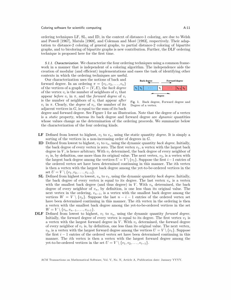
Our characterization uses the notions of back andforward degree. In an ordering π = {v1, v2, . . . , vn}of the vertices of a graph G = (V,E), the back degreeof the vertex vi is the number of neighbors of vi thatappear before vi in π, and the forward degree of viis the number of neighbors of vi that appear aftervi in π. Clearly, the degree of vi, the number of itsadjacent vertices in G, is equal to the sum of its backdegree and forward degree. See Figure 1 for an illustration. Note that the degree of a vertexis a static property, whereas its back degree and forward degree are dynamic quantitieswhose values change as the determination of the ordering proceeds. We summarize belowthe characterization of the four ordering kinds.

LF Defined from lowest to highest, v1 to vn, using the static quantity degree. It is simply asorting of the vertices in a non-increasing order of degrees in G.

ID Defined from lowest to highest, v1 to vn, using the dynamic quantity back degree. Initially,the back degree of every vertex is zero. The first vertex v1, a vertex with the largest backdegree in V , is hence arbitrary. With v1 determined, the back degree of every neighbor ofv1 is, by definition, one more than its original value. The next vertex, v2, is a vertex withthe largest back degree among the vertices U = V \{v1}. Suppose the first i−1 entries ofthe ordered vertex set have been determined continuing in this manner. The ith vertexis then a vertex with the largest back degree among the yet-to-be-ordered vertices in theset U = V \ {v1, v2, . . . , vi−1}.

SL Defined from highest to lowest, vn to v1, using the dynamic quantity back degree. Initially,the back degree of every vertex is equal to its degree. The last vertex vn is a vertexwith the smallest back degree (and thus degree) in V . With vn determined, the backdegree of every neighbor of vn, by definition, is one less than its original value. Thenext vertex in the ordering, vn−1, is a vertex with the smallest back degree among thevertices W = V \ {vn}. Suppose the last n − i − 1 entries of the ordered vertex sethave been determined continuing in this manner. The ith vertex in the ordering is thena vertex with the smallest back degree among the yet-to-be-ordered vertices in the setW = V \ {vn, vn−1, . . . , vi+1}.

DLF Defined from lowest to highest, v1 to vn, using the dynamic quantity forward degree.Initially, the forward degree of every vertex is equal to its degree. The first vertex v1 isa vertex with the largest forward degree in V . With v1 determined, the forward degreeof every neighbor of v1 is, by definition, one less than its original value. The next vertex,v2, is a vertex with the largest forward degree among the vertices U = V \{v1}. Supposethe first i − 1 entries of the ordered vertex set have been determined continuing in thismanner. The ith vertex is then a vertex with the largest forward degree among theyet-to-be-ordered vertices in the set U = V \ {v1, v2, . . . , vi−1}.



1

d fb e ih g jc d fb e ih

2

1 3

2

a

c

h

bd

ejg

ifa

431

3

j

4

i

2

h

2

g

3

fe

42

dc

2

b

42

a

2 3 41

c

d

f

e

2

a c d fb ge

2

jih

3 344

1 1 3 23 3 −1

Degrees

Positions

Buckets

1 1 23 2 5

Degrees

Positions

Buckets

31

4 2 2 1

−1

g

i

ba

j

Candidate

Candidate

g ja c

h

g

f

j

i e

c

d

b

a

Fig. 2. Data structure for efficient implementation of the ordering techniques SL, DLF and ID. The SLordering case is illustrated here, where the left subfigure shows the initial condition, and the right subfigureshows the condition after vertex h is ordered (last in a list not shown here).

5.1.2. Computation. Besides serving as a conceptual framework, the above characteriza-tion of the orderings also facilitates the design and implementation of fast algorithms forcomputing (obtaining) the orderings.

Consider an LF ordering for example. Since the degree of a vertex in a connected graphG = (V,E) is an integer in the interval [1,∆], where ∆ ≤ |V | is the maximum degree inthe graph, an LF ordering can be obtained in linear time by bucket-sorting the verticesaccording to their degrees in G using an auxiliary array of size ∆.

An ID, DLF or SL ordering can be computed in a similar fashion, except now the backor forward degrees of adjacent vertices need to be updated every time a vertex is selected tobe placed in the ordered list. The update involves relocating the neighbors of the selectedvertex into appropriate buckets, but the work can still be made proportional to the degree-1of the vertex by using suitable pointer techniques. Figure 2 illustrates the technique used inColPack to achieve this. The illustration is for SL ordering, but the same principle is usedfor DLF and ID orderings as well. The “Positions” pointer array there is used to locate theposition of a vertex in the “Buckets” array, which maintains the relevant degree information,in this case back degree, in constant time. At a given step of the ordering, the last vertex inthe first non-empty bucket in the array “Buckets” is the “Candidate” vertex, the vertex tobe ordered at that step. Once the candidate vertex is ordered (removed from the Buckets-data structure), each of its neighbors need to be moved to a new bucket to reflect thatthe back degree of each is decremented by one. In order to achieve this with minimal datamovement, the neighbor is first swapped with the last element in the current bucket, andthen it is simply moved to the new bucket. The left subfigure in Figure 2 depicts the initial



condition, where vertices are bucket sorted according to their back degrees (which initiallyis the same as degrees). The right subfigure shows the updated data structure after thevertex with the smallest degree, h, has been ordered. In this (and similar) manner, eachof the three ordering variants SL, DLF and ID is implemented in ColPack such that itsruntime is O(|E|). In all of the ordering routines in ColPack, ties are broken arbitrarily.

5.2. The coloring number of a graph

A general heuristic intuition behind the ordering techniques being discussed is that in thecourse of a greedy algorithm that colors the vertices in the order v1 to vn, vertices thatare more constrained in the choice of colors get colored early, making it more likely for thealgorithm to use fewer colors compared to, say, an arbitrary order. In contrast to LF, ID andDLF ordering, an SL ordering, however, goes a step further—it minimizes a mathematicallywell defined objective.

Given a graph G and a vertex ordering π, let Bπ(G) denote the maximum back degree inthe ordering π, and χ(G, π) denote the number of colors used by a greedy algorithm thatuses the ordering π to color G. Further, let ∆(G) denote the maximum degree in G andχ(G) denote the chromatic number of G, the optimal (least) number of colors required tocolor G. Then, it is fairly easy to see that the relationship

χ(G, π) ≤ Bπ(G) + 1, (1)

always holds, and can be extended at both ends as follows:

χ(G) ≤ χ(G, π) ≤ Bπ(G) + 1 ≤ ∆(G) + 1. (2)

Now, different vertex orderings could result in different maximum back degrees. An SL-ordering gives the minimum maximum back degree, not only among the four ordering vari-ants being discussed, but among all possible orderings. That is,

BSL(G) = minπBπ(G), (3)

where the minimum is taken over the n! possible vertex orderings of the graph G [Matulaet al. 1972; Finck and Sachs 1969]. The quantity BSL(G)+1 is a graph parameter (a uniquevalue for a given graph) known as the coloring number col(G) of G [Erdos and Hajnal 1966],so named due to its connection to coloring, although its definition, as presented here, isindependent of coloring.

Noting that the size of the largest clique in G, the clique number ω(G), is an obvious lowerbound on the chromatic number χ(G), the relationship in Equation (2) can be extended atthe lower end in the following manner:

ω(G) ≤ χ(G) ≤ χ(G, π) ≤ Bπ(G) + 1 ≤ ∆(G) + 1. (4)

And the relationship among the clique number, the chromatic number, the coloring number,the maximum back degree, and the maximum degree for any given graph G and vertexordering π can be summarized in the following manner:

ω(G) ≤ χ(G) ≤ col(G) = BSL(G) + 1 ≤ Bπ(G) + 1 ≤ ∆(G) + 1. (5)

Note that although BSL(G) ≤ Bπ(G) holds for any graph G and ordering π, no statementcan be made regarding the relationship between the actual number of colors output by agreedy algorithm that uses an SL ordering and the number output by an algorithm thatuses the ordering π. In other words, the expression χ(G,SL) could be less than, greaterthan, or equal to the expression χ(G, π) for an ordering π that is not SL. Moreover, sincemultiple vertices in a graph could have the same degree value, none of the ordering variantsLF, ID, DLF and SL is uniquely defined for a given graph. Instead each defines a classof orderings, and a tie-breaking strategy is needed to determine a specific member in each



class. For instance, two vertex orderings π1 and π2 could be distinct and yet each be an SLordering—and χ(G, π1) could differ from χ(G, π2). However, no matter how ties are brokenin an SL ordering, all such orderings give the same BSL(G), and hence the coloring numberis uniquely determined.

5.3. Relationship between coloring number and other graph parameters

The coloring number col(G) of a graph has interesting connection with several graph con-cepts beyond coloring, including degeneracy, core and arboricity [Matula et al. 1972; Szek-eres and Wilf 1968; Lick and White 1970; Diestel 2000; Gebremedhin et al. 2005]. At theheart of this connection lies a relationship between the parameter col(G) and yet anothergraph parameter, the maximum minimum degree in an induced subgraph of G, where themaximum is taken over all possible induced subgraphs of G. Specifically, let

κ = maxH⊆G

δ(H), (6)

where H ⊆ G denotes a nonempty induced subgraph of G and δ(H) denotes the minimumdegree in H. Matula [1972] and Szekeres and Wilf [1968], independently, showed that

col(G) = κ+ 1. (7)

In the social and biological network literature, this quantity is known as the k-core.

5.4. Saturation Degree-based coloring

Saturation Degree ordering, due to Brelaz [1979], is another known ordering technique forgreedy coloring. It can be best viewed in contrast to the ID ordering technique: in a coloringalgorithm that uses an ID ordering, the ith vertex is a vertex with the largest numberof already colored adjacent vertices, whereas in an algorithm that uses an SD orderingit is a vertex that has the largest number of distinctly colored adjacent vertices. Clearly,the characterization of an SD ordering cannot be separated from the rest of the coloringalgorithm, and the ordering is non-amenable for a linear-time implementation in the size ofthe graph. For these reasons we chose not to include it in ColPack. Turner [1988] has shownthat using careful choice of data structures, a coloring algorithm that in effect employsan SD ordering can be implemented such that its complexity is O(|E| log |V |). We haveimplemented such an algorithm and we will report results on it in the experiments discussedin Section 8.

5.5. Extension of degree-based orderings to other coloring problems

We have adapted the ordering techniques LF, ID, DLF and SL—the characterizations givenin section 5.1.1—to suit the various specialized coloring problems supported by ColPack.The adaptation involves extending the notion of degree, since the specialized algorithmsinvolve visits to the distance-2 neighborhood of a vertex in a graph and/or the coloringis performed on a bipartite graph. In ColPack, each ordering technique is implemented insuch a way that its time complexity is upper-bounded by the complexity of the coloringalgorithm for which it is designed.

5.6. Coloring-based ordering

Let φ : V → {1, 2, . . . , C} be a distance-1 coloring of a graph G = (V,E) on n vertices. Nowconsider an ordering π = {v1, v2, . . . , vn} in which vertices that belong to a color class—those vertices with the same color—are always listed consecutively, i.e., if φ(vi) = φ(vk) = c,then φ(vj) = c for i < j < k. A greedy algorithm that uses the ordering π obtains a newdistance-1 coloring of G using C or fewer colors. Culberson [1992] applied this propertyof the greedy coloring algorithm in his method called Iterative Greedy (IG) to attempt tosuccessively reduce the number of colors used. As long as vertices of a color class are listed



consecutively, there is a degree of freedom in the way in which the color classes themselvescan be ordered. One of the better strategies used in Culberson’s IG method is to orderthe classes in reverse order of their introduction, i.e., the ordering π is obtained by listingvertices of color C consecutively, followed by vertices of color C − 1, and so on, and finallyvertices of color 1.

We truncate this variant of Culberson’s IG method to just two iterations, where the firstiteration is used to merely determine an ordering for the second, where a fresh coloring isobtained. Specifically, a coloring-based ordering routine available in ColPack takes as inputa coloring φ of a graph and gives as output a vertex ordering π based on a reverse listingof the color classes in φ. ColPack has coloring-based ordering routines for distance-1 anddistance-2 coloring of general graphs and for partial distance-2 coloring and bicoloring ofbipartite graphs. We note that a back-tracking algorithm similar in spirit to IG methodbut with better performance in terms of number of colors has been proposed recently in[Bhowmick and Hovland 2008].

6. OTHER FUNCTIONALITIES IN COLPACK

Besides coloring and ordering capabilities, ColPack contains two classes of functionalities.

6.1. Recovery routines

Recall that the last step in the procedure for sparse derivative computation (Algorithm 1,Section 2) involves recovering the numerical values of the entries of a derivative from a com-pressed representation. The following recovery routines are currently available in ColPack:

— Recovery routines for Hessian computation, both for direct (via star coloring) andsubstitution-based (via acyclic coloring) methods. The recovery routine for a substitution-based method uses the two-colored trees the acyclic coloring algorithm maintains duringits execution. This routine—as well as the corresponding routine for a direct method—hasbeen described and analyzed in detail in a recent paper [Gebremedhin et al. 2009].

— Recovery routines for unidirectional, direct Jacobian computation, both for column-wiseand row-wise computation (via appropriate distance-2 coloring).

— Recovery routines for bidirectional, direct Jacobian computation via star bicoloring.

To facilitate the use of ColPack by other scientific computing software tools, each recov-ery routine in ColPack comes in three variations corresponding to three different formatsin which the values in a “de-compressed” derivative matrix are returned. These three for-mats are: Row Compressed Format (which is used among others by ADOL-C [Walther andGriewank 2012]), Coordinate Format and Sparse Solvers Format1.

6.2. Graph reading routines

In ColPack, we use the Compressed Sparse Row (CSR) data structure to store graphs.CSR is a widely used data structure in scientific computing. It consists essentially of twoone-dimensional integer arrays (vectors), one corresponding to vertices and the other toedges. Indices to these arrays correspond to vertex or edge identifiers. For each vertex, theadjacency list of the vertex is stored in consecutive locations in the edge array and thevertex array is used to point to the beginning and the end.

As a supporting functionality, ColPack provides routines for constructing bipartite graphdata structures (for Jacobians) and adjacency graph data structures (for Hessians) fromfiles specifying matrix sparsity structures. Various file formats, including formats used byMatrix Market [Boisvert et al. 1996], Harwell-Boeing [Duff 1992] and MeTis [Karypis andKumar 1998] are supported.

1www.intel.com/software/products/mkl/docs/webhelp/appendices/mkl appA SMSF.html



Fig. 3. Overview of the structure of the major classes in ColPack. A solid arrow indicates aninheritance-relationship, and a broken arrow indicates a uses-relationship.

7. COLPACK’S ORGANIZATION AND USAGE

ColPack is written in an object-oriented fashion in C++. It is designed to be modular andextensible. Figure 3 gives an overview of the structure of the major classes of ColPack.

The entire ColPack package is under the ColPack namespace. Two core classes,GraphCore and BipartiteGraphCore, are used to store the general graph and bipar-tite graph, respectively, data structures in CSR format. The classes GraphCore andBipartiteGraphCore are abstract (pure virtual) with no methods to manipulate data.The classes GraphInputOutput and BipartiteGraphInputOutput, which inherit the classesGraphCore and BipartiteGraphCore, respectively, contain routines for building adjacencygraphs and bipartite graphs from files specifying matrix sparsity structures.

The class GraphInputOutput starts up an inheritance chain collectively containing im-plementations of various coloring and ordering algorithms for general graphs. For a similarpurpose on bipartite graphs, the class BipartiteGraphInputOutput starts up two sepa-rate inheritance chains, one concerning partial distance-2 coloring and the other bicoloring.ColPack functions that a user typically needs to call directly are made available via theappropriate Interface classes:

— GraphColoringInterface,— BipartiteGraphPartialColoringInterface, and— BipartiteGraphBicoloringInterface



The classes HessianRecovery, JacobianRecovery1D and JacobianRecovery2D housethe appropriate routines for recovering a derivative matrix from its compressed represen-tation. The class RecoveryCore, which is inherited by each of the three classes, containsfunctions for allocating and deallocating memory associated with the recovery routines.

A description of the major functions in the interface classes of ColPack as well as otherrelated documentation is available at the package’s distribution website.

In the appendix, we have included two code samples that illustrate how ColPack’s capa-bilities are used.

8. EXPERIMENTAL ANALYSIS

It is useful to know how effective in practice the various ordering techniques discussed inSection 5 are and how they compare against each other when used in the context of thevarious greedy coloring algorithms discussed in Section 4. We present in this section a setof experimental results that illustrate different aspects of the ordering techniques as well asof the encompassing coloring algorithms. We begin in Sections 8.1 and 8.2 by discussing theexperimental setup. We then present results on distance-1 coloring in Section 8.3; results ondistance-2, star and acyclic coloring in Section 8.4; and results on coloring bipartite graphsin Section 8.5.

8.1. Data set

We sought to include in the testbed a wide variety of graph structures. The testbed weassembled consists of 30 graphs grouped in two categories.

The first category contains ten graphs obtained from the University of Florida MatrixCollection [Davis and Hu 2011]. These graphs originate from various areas in scientificcomputing, including structural engineering, civil engineering, and automotive and shipindustry.

The second category consists of twenty synthetically generated graphs representing fourdifferent graph “classes”. The first represented class is that of planar graphs. The graphs,more specifically, are maximally planar—the degree of every vertex is at least five—and aregenerated using the expansion method described in [Morgenstern and Shapiro 1991]. Theremaining three classes of graphs are generated using the R-MAT algorithm [Chakrabartiand Faloutsos 2006]. The R-MAT algorithm, using various parameter configurations, allowsfor generating graphs with varying properties in terms of degree distributions and localdensity. The three classes we generated are Erdos-Renyi random, and two kinds of small-world type graphs (we use the descriptor small-world in a loose sense).

The R-MAT algorithm works by recursively subdividing the adjacency matrix of thegraph to be generated (a |V | by |V | matrix) into four quadrants (1, 1), (1, 2), (2, 1) and(2, 2), and distributing the |E| edges within the quadrants with specified probabilities. Thedistribution is determined by four non-negative parameters (a, b, c, d) whose sum equals one.Initially, every entry of the adjacency matrix is zero (no edges added). The algorithm placesan edge in the matrix by choosing one of the four quadrants (1, 1), (1, 2), (2, 1), or (2, 2)with probabilities a, b, c, or d, respectively. The chosen quadrant is then subdivided intofour smaller partitions and the procedure is repeated until a 1×1 quadrant is reached, wherethe entry is incremented (the edge is placed). The algorithm repeats the edge generationprocess |E| times to create the desired graph G = (V,E).

The Erdos-Renyi random graphs in our testbed are generated by letting each of the fourR-MAT parameters be 0.25. The first type of small-world graphs is generated using theset of parameters (0.45, 0.15, 0.15, 0.25), whereas the second type is generated using theparameter set (0.55, 0.15, 0.15, 0.15). The parameter combination in the second type resultsin graphs with larger maximum degrees (and also denser local subgraphs) compared to the



Table III. Structural statistics and distance-1 coloring results on the scientific comput-ing (sc) graphs.

Name |V| |E| ∆ BSL ω SL ID LF DLF N SDsc1 (msdoor) 415,863 9,912,536 76 35 21 35 38 42 41 42 41sc2 (ldoor) 952,203 22,785,136 76 35 21 35 35 42 38 42 42sc3 (shipsec1) 140,874 3,836,265 101 48 24 38 37 54 47 48 45sc4 (shipsec5) 179,860 4,966,618 125 48 24 39 39 48 47 50 46sc5 (pkustk11) 87,804 2,565,054 131 48 36 42 42 54 50 66 48sc6 (ct20stif) 52,329 1,323,067 206 47 47 47 47 47 47 49 48sc7 (pwtk) 217,918 5,708,253 179 36 24 35 40 42 42 48 41sc8 (pkustk13) 94,893 3,260,967 299 42 36 42 42 45 44 57 49sc9 (nasasrb) 54,870 1,311,227 275 36 24 36 34 40 37 41 40sc10 (bmw3 2) 227,362 5,530,634 335 42 36 36 39 48 42 48 44

Table IV. Structural statistics and distance-1 coloring results on the synthetic (planar,Erdos-Renyi random, small-world) graphs.

Name |V| |E| ∆ BSL ω SL ID LF DLF N SDp1 102,093 306,273 35 5 4 5 6 6 6 8 7p2 204,049 612,141 29 5 3 6 6 6 6 8 7p3 407,521 1,222,557 29 5 4 6 6 6 6 8 7p4 819,502 2,458,500 32 5 4 6 6 6 6 9 7p5 1,625,972 4,877,910 37 5 4 6 6 7 6 8 7er1 200,000 2,468,251 100 26 3 16 16 16 15 17 17er2 200,000 4,443,541 173 48 3 23 23 22 21 24 24er3 200,000 6,910,713 253 77 3 30 31 30 29 32 32er4 200,000 8,882,591 322 100 3 36 37 36 34 37 38er5 200,000 11,347,805 410 128 4 43 43 43 41 44 45sw1 200,000 2,422,134 534 31 5 18 19 19 20 32 20sw2 200,000 4,350,665 954 57 8 27 27 28 29 46 29sw3 200,000 6,747,685 1,380 89 10 36 36 37 39 61 38sw4 200,000 8,656,160 1,783 115 12 43 43 45 46 72 46sw5 200,000 11,030,782 2,222 147 14 51 51 53 54 85 53sw6 200,000 2,347,871 3,754 156 30 55 56 58 59 78 56sw7 200,000 4,152,742 5,596 248 43 83 83 88 87 114 83sw8 200,000 6,343,766 7,505 334 67 112 111 117 118 154 110sw9 200,000 8,055,368 8,893 416 93 132 130 139 140 178 129sw10 200,000 10,148,629 10,329 512 114 154 150 159 162 209 156

first type. All of the R-MAT graphs were generated using the GTgraph Synthetic GraphGenerator Suite2. Duplicate edges and self loops were removed.

8.2. Properties of the test graphs

We provide in Tables III and IV basic structural properties as well as some computedquantities in the test graphs. The information in the two tables is catalogued in four parts:

— the first part shows abbreviated names of the graphs: scientific computing (sc), planar(p), Erdos-Renyi (er), and small-world (sw).

— |V | and |E| show the number of vertices and edges in the input graph G.— ∆ shows the maximum degree in G; BSL shows the minimum maximum back degree inG; and ω shows the clique number of G.

— the last six columns list the number of colors used by the greedy distance-1 coloringalgorithm while employing the ordering variants Smallest Last (SL), Incidence Degree(ID), Largest First (LF), Dynamic Largest First (DLF), Natural (N) and SaturationDegree (SD). (Natural corresponds to the order in which vertices appear in the inputgraph.)

2http://www-static.cc.gatech.edu/kamesh/GTgraph/



We will shortly discuss the numbers in these last six columns in some detail, but first wecomment on a few other aspects in the tables.

As discussed in Section 5.2, the minimum maximum back degree (BSL) is computed usingthe Smallest Last ordering. It is equal to the coloring number col(G) minus one, and is atighter upper bound on the chromatic number χ(G) than the bound ∆ + 1.

The clique number ω(G), which is a lower bound on the chromatic number χ(G), is NP-hard to compute. We computed it using an exact, exhaustive search algorithm that findsthe largest clique to which a vertex belongs. To compute the largest clique to which a givenvertex belongs, we implemented the per-vertex clique finding algorithm described in [Turner1988]. We pruned the exhaustive search (for the entire graph) by maintaining the size of thelargest clique found so far and invoking the clique-finding algorithm for a particular vertexonly if the degree of that vertex is larger than the current maximum clique. This prunedalgorithm, whose worst-case complexity is still exponential, is quite fast in practice. As anexample, on a typical er graph, the algorithm took a few seconds, and on a typical swIgraph, it took a few dozens of seconds.

Finally, the SD coloring algorithm (whose results are listed in the last column in Tables IIIand IV) is our implementation of the algorithm described by Turner [1988]. The algorithmwas briefly discussed in Section 5.4, and it is to be recalled that it is not included inColPack.

Compute platform. All of the experiments in this paper were run on an Intel Nehalemmicroarchitecture equipped with Intel(R) Core(TM) i7 CPU 860 processors running at2.80GHz. The system has 4 cores and 8 threads, but the experiments were run on singleprocessor and a single thread. The total memory size of the system is 16 GB, with 4 × 32KB Instruction and 4 × 32 KB Data Level-1 cache, 4 × 256 KB Level-2 cache, and 8 MBshared Level-3 cache. The operating system is GNU/Linux, and the compiler is g++.

8.3. Results on distance-1 coloring

8.3.1. Number of colors used. As mentioned earlier, the last six columns in Tables III andIV list the number of colors χ(G, π) used by the greedy algorithm for distance-1 coloringwhen various ordering techniques π are used. For each graph, the smallest χ(G, π), amongthe six ordering variants π considered, is shown in boldface. We highlight a few generalobservations on the results shown in the two tables.

— In nearly every one of the graphs from the scientific computing category, either SL or IDordering gave the fewest colors. The difference between the two is in turn quite small,usually one or two colors, whereas the reduction they offer compared to LF, DLF and Nis relatively large.

— As expected from theory, the greedy algorithm using SL ordering colored planar graphsusing at most six colors.

— For the Erdos-Renyi random graphs, although the various ordering techniques in generalgave similar number of colors, DLF gave the fewest.

— For the small-world graphs, SL, ID, LF, and DLF reduced the number of colors comparedto Natural ordering, but showed little difference among each other, with SL or ID onceagain giving the fewest colors.

— SD ordering almost invariably used more colors than ID and SL ordering in the graphsfrom both test sets. (This is rather surprising since SD ordering employs a vertex selectioncriteria that intuitively seems more accurate than ID ordering in capturing color choiceconstraints. In our implementation of the SD ordering, ties are broken in favor of thevertex with larger degree; in all other ordering techniques in ColPack ties are brokenarbitrarily.)



er1 er2 er3 er4 er5

1

1.5

2

2.5

3

3.5

4

Val

ues

norm

aliz

ed b

y B

SL

∆ BN

BSL

(a) Degrees, random

er1 er2 er3 er4 er5

0

5

10

15

20

25

30

35

Val

ues

norm

aliz

ed b

y ω

BSL N SL ω

(b) Colors, random

sw1 sw2 sw3 sw4 sw50

2

4

6

8

10

12

14

16

18

Val

ues

norm

aliz

ed b

y B

SL

∆ BN

BSL

(c) Degrees, small-world I


2

4

6

8

10

12

Val

ues

norm

aliz

ed b

y ω

BSL N SL ω

(d) Colors, small-world I


0

5

10

15

20

25

Val

ues

norm

aliz

ed b

y B

SL

∆ BN

BSL

(e) Degrees, small-world II


1

2

3

4

5

6

7

Val

ues

norm

aliz

ed b

y ω

BSL N SL ω

(f) Colors, small-world II

Fig. 4. Left: Maximum degree ∆, maximum back degree using Natural ordering BN , and maximum backdegree using Smallest Last ordering BSL, each normalized by BSL. Right: the number of colors by thegreedy algorithm using Natural ordering (N) and Smallest Last ordering (SL), the minimum maximumback degree BSL, and the clique number ω, each normalized by ω. Test graphs: synthetic (random andsmall-world)



8.3.2. Maximum back degrees, comparison with optimal values. Recall from Equations (4) and(5) in Section 5 that:

— the maximum back degree Bπ(G) plus one is a tighter upper bound on the number ofcolors χ(G, π) than the maximum degree ∆(G) plus one;

— the minimum maximum back degree is attained when Smallest Last ordering is used; and— the clique number ω(G) is a lower bound on the chromatic number χ(G).

The results reported in Tables III and IV readily reflect several aspects of these facts.To provide further insight into the relative proximity among the various quantities, we

present in Figure 4 plots that show how the various quantities relate to each other. The plotsare for the R-MAT generated synthetic graphs (random and small-world type). In all thosefigures, we use Smallest Last ordering as the representative effective ordering technique andcompare it against Natural ordering. The left subfigures show curves corresponding to threequantities: maximum degree ∆(G), maximum back degree using Natural ordering BN (G),and maximum back degree using Smallest Last ordering BSL(G) (the minimum maximumback degree in the graph). Each of the three quantities is normalized by BSL(G). The rightsubfigures show curves corresponding to four quantities: the number of colors χ(G,N) usedby the greedy algorithm when Natural ordering is employed (denoted by N in the figure),the number of colors χ(G,SL) used by the greedy algorithm when Smallest Last orderingis used (denoted by SL in the figure), the minimum maximum back degree BSL(G), andthe clique number ω(G). Each quantity is normalized by ω(G).

For a given graph G, let rχ(G) denote the ratio between the approximate solutionχ(G,SL) and the optimal solution χ(G) (that is, rχ(G) ≡ χ(G,SL)

χ(G) ). Similarly, let rω(G) ≡χ(G,SL)ω(G) . Clearly rχ(G) ≤ rω(G). The results in Figure 4 show that the ratio rω is relatively

small indicating that the approximation ratio rχ is even smaller. The table below summa-rizes the observed maximum value on the ratio rω in each of the five graph groups used inthe experiments:

sc p er sw I sw IIrω is at most 1.8 2 10 4 2

The ratio rω is the highest for the group er because these graphs (random) are the mostunstructured among all in the testbed.

Another observation to be made from Figure 4 is that the upper bound ∆(G) + 1 cus-tomarily given for χ(G) is often several factors larger than the bound BSL(G) + 1. Thefollowing table summarizes this observation, again for all test graph groups:

sc p er sw I sw II∆(G)BSL(G) could be as high as 8 6 4 18 25

8.3.3. Run time. The fact that the greedy coloring algorithm with an ordering such as SLquickly computes a solution so close to optimal cannot be overstated. As discussed earlier,the time complexity of the greedy distance-1 coloring algorithm in ColPack is linear in thesize of the graph (Section 4), and each of the ordering techniques LF, DLF, ID and SLis implemented in ColPack so that its time complexity is also linear (Section 5). Figure 5shows the observed total execution times (i.e. ordering plus coloring) in seconds for distance-1 coloring while using the ordering techniques N, LF, ID, SL, and DLF on the syntheticgraphs. Also shown in the same figure is the total execution time for the SD ordering-basedcoloring algorithm (Turner’s algorithm). It can be seen that the N and LF ordering basedcoloring algorithms take about the same time and are the fastest. These are closely followedby the algorithms using ID, SL and DLF ordering, which in turn take about the same time.And, finally, it can be seen that coloring based on SD ordering is significantly slower than



p1 p2 p3 p4 p50

0.5

1

1.5

2

2.5

Tim

e (s

ec)

SD DLF SL

ID LF N

(a) Planar

er1 er2 er3 er4 er50

0.5

1

1.5

2

2.5

Tim

e (s

ec)

SD DLF SL

ID LF N

(b) Erdos-Renyi


0.5

1

1.5

2

2.5

3

3.5

Tim

e (s

ec)

SD DLF SL

ID LF N

(c) Small-world I


0.5

1

1.5

2

2.5

3

3.5

4

4.5

Tim

e (s

ec)

SD DLF SL

ID LF N

(d) Small-world II

Fig. 5. Runtime of distance-1 coloring using Natural (N), Largest First (LF), Incidence Degree (ID), Small-est Last (SL), and Dynamic Largest First (DLF) ordering (all five in ColPack), and Saturation Degree (SD)ordering (not in ColPack).

the ColPack algorithms based on LF, ID, SL and DLF ordering. Note that with the ColPackalgorithms, even the largest graphs (having several millions of edges) are colored in just asecond or less.

8.3.4. Coloring-based ordering results. Experiments we did on coloring-based ordering (dis-cussed in Section 5.6) showed that if one starts with a Natural ordering, re-coloring reducesthe number of colors used. The magnitude of reduction is comparable to what one wouldsee in using SL ordering compared to Natural ordering. If one starts with an ordering suchas Smallest Last, however, re-coloring provides almost no further reduction in number ofcolors. We omit the results here for space considerations.

8.4. Results on distance-2, star and acyclic coloring

8.4.1. Impact of ordering techniques on number of colors. We have conducted experiments usingthe degree-1 and degree-2 versions of the various ordering techniques (LF, DLF, SL, ID)in the context of distance-2, star and acyclic coloring. We again omit the results for spaceconsiderations, but point out two major observations we made from the results:

— Compared to Natural ordering, the various degree-1-based ordering techniques reduce thenumber of colors in the distance-2, star and acyclic coloring algorithms. The reduction is



sc1 sc2 sc3 sc4 sc5 sc6 sc7 sc8 sc9 sc100

50

100

150

200

250

300

350

Num

ber

of colo

rs

D2 S A D1

Fig. 6. Number of colors used by the greedy algorithms for distance-1 (D1), acyclic (A), star (S) anddistance-2 (D2) coloring on the scientific computing graphs. In all cases, SL ordering was used.

Table V. Number of colors used by the distance-1 (D1), acyclic (A), star and distance-2 (D2) coloring algorithms on the synthetic graphs. In all cases, Smallest Last orderingwas used.

Name D1 A S D2 ∆ Name D1 A S D2 ∆p1 5 7 16 36 35 er1 16 32 104 233 100p2 6 7 18 30 29 er2 23 57 230 606 173p3 6 7 20 30 29 er3 30 90 423 1,280 253p4 6 7 22 33 32 er4 36 117 605 1,974 322p5 6 7 22 38 37 er5 43 151 854 3,022 410

sw1 18 54 211 569 534 sw6 55 298 885 3,755 3,754sw2 27 97 418 1,348 954 sw7 83 609 1,534 6,180 5,596sw3 36 153 733 2,669 1,380 sw8 112 996 2,179 9,096 7,505sw4 43 201 1,009 3,870 1,783 sw9 132 1,108 2,645 11,089 8,893sw5 51 262 1,373 5,501 2,222 sw10 154 1,888 3,430 14,101 10,329

analogous to the reduction we saw in the distance-1 coloring algorithm (in Section 8.3);in most cases, SL (or ID) ordering gave the fewest colors in each of the coloring variants.

— The degree-2 versions of the ordering techniques do not offer significant reduction innumber of colors compared to the degree-1 versions, whereas they incur considerableincrease in runtime.

8.4.2. Cross-comparison. An issue of separate interest is how the greedy algorithms inColPack for distance-1, acyclic, star, and distance-2 coloring compare against each other interms of number of colors used and runtime.

Number of colors. Figure 6 shows results on the scientific computing graphs comparingthe four coloring variants against each other in terms of number of colors used when theordering technique is fixed to be SL. A similar comparison for the synthetic graphs isprovided in a tabular format in Table V. We highlight a few observations gleaned from theresults contained in the figure and the table.

— In terms of number of colors used, acyclic coloring is closer to distance-1 coloring thanit is to distance-2 coloring, and star coloring is closer to distance-2 coloring than it is todistance-1 coloring.

— For planar graphs, the acyclic coloring algorithm in ColPack uses about the same numberof colors as the distance-1 coloring algorithm (to be exact, the acyclic coloring algorithmused seven colors whereas the distance-1 coloring algorithm used at most six colors). This



p1 p2 p3 p4 p5

0

1

2

3

4

5

6

7

8

Tim

e(se

c)

S A D2 D1

(a) Planar

er1 er2 er3 er4 er5

0

100

200

300

400

500

600

700

800

Tim

e(se

c)

S A D2 D1

(b) Erdos-Renyi

sw1 sw2 sw3 sw4 sw5

0

500

1000

1500

Tim

e(se

c)

S A D2 D1

(c) Small world I


0

500

1000

1500

2000

2500

3000

3500

4000

4500

Tim

e(se

c)

S A D2 D1

(d) Small world II

Fig. 7. Runtime of distance-1 (D1), acyclic (A), star (S) and distance-2 (D2) coloring on the syntheticgraphs. In all cases, Smallest Last ordering was used.

result is in close agreement with theory [Borodin 1979], and shows that the heuristic inColPack provides nearly optimal solutions.

— Again for planar graphs, the star coloring algorithm in ColPack uses a number of colorsin the range between sixteen and twenty-two. The optimal number of colors needed tostar color a planar graph is known to lie between ten and twenty [Albertson et al. 2004].This indicates that the ColPack-algorithm is close to optimal for such graphs.

— The maximum degree ∆(G) + 1 in a graph is a lower bound on the number of colorsneeded to distance-2 color a graph. As the data in Table V shows, the ColPack algorithmfor distance-2 coloring finds optimal solution for planar graphs. Further, for the otherthree types of test graphs, it can be seen that the ratio between the number of colors usedin distance-2 coloring and the quantity ∆(G) is relatively small (e.g., 1.37 for sw10, 2.48for sw5, and 7.37 for er5), indicating that the algorithm yields solutions reasonably closeto optimal. The corresponding ratios for the scientific computing graphs (Figure 6) rangefrom 1.00 to 1.03, indicating that the solutions for all practical purposes are optimal.

Run time. As mentioned in Section 4, the star, acyclic and distance-2 coloring algorithmsin ColPack have nearly the same time complexity, O(|V |·d2), with varying magnitudes of theconstants. Since star and acyclic coloring involve substantial work related to bookkeeping oftwo-colored subgraphs (more for star coloring than acyclic coloring), their practical runtime



Table VI. Structural statistics and partial distance 2 coloring (column-wise) results onvarious scientific computing graphs.

Name |V1| |V2| |E| ∆(V1) SL ID LF DLF Ncre a 3,516 7,248 18,168 360 360 360 360 360 360ken 11 14,694 21,349 49,058 122 125 124 128 122 130ken 13 28,632 42,659 97,246 170 171 171 174 170 176maros r7 3,136 9,408 144,848 48 83 90 70 114 74cre d 8,926 73,948 246,614 808 808 808 808 808 813ken 18 105,127 154,699 358,171 325 325 326 328 325 330af23560 23,560 23,560 460,598 21 42 42 43 59 44e40r0100 17,281 17,281 553,562 62 70 71 87 85 95cage11 39,082 39,082 559,722 31 64 67 67 70 81cage12 130,228 130,228 2,032,536 33 67 72 73 79 96

Table VII. Structural statistics and partial distance 2 coloring (row-wise) results onvarious scientific computing graphs.

Name |V1| |V2| |E| ∆(V2) SL ID LF DLF Ncre a 3,516 7,248 18,168 14 14 14 14 14 16ken 11 14,694 21,349 49,058 3 4 4 4 5 5ken 13 28,632 42,659 97,246 3 4 5 5 5 4maros r7 3,136 9,408 144,848 46 80 88 100 113 72cre d 8,926 73,948 246,614 13 15 15 13 14 15ken 18 105,127 154,699 358,171 3 4 5 5 5 5af23560 23,560 23,560 460,598 21 42 43 43 60 43e40r0100 17,281 17,281 553,562 62 70 71 85 86 87cage11 39,082 39,082 559,722 31 64 67 67 70 81cage12 130,228 130,228 2,032,536 33 67 72 73 79 96

is expected to be higher than that of distance-2 coloring. These expectations are confirmedby the observed execution times depicted in Figure 7, which shows a plot of the total(coloring plus ordering) execution times on the synthetic test graphs for the three coloringproblems and the distance-1 coloring problem (whose complexity is O(|V | · d1)) while usingthe SL ordering in each case.

8.5. Results on coloring bipartite graphs

8.5.1. Partial distance-2 coloring (unidirectional matrix partition). Versions of the ordering tech-niques LF, DLF, ID and SL tailored for the partial distance-2 coloring of bipartite graphs(on either of the two vertex sets of the bipartite graph) are available in ColPack. Tables VIand VII show results on these ordering techniques when applied to various scientific com-puting graphs obtained from the University of Florida Matrix Collection. The results showthat the ordering techniques reduce the number of colors compared to natural ordering.The benefit due to ordering here is similar to that seen in the distance-1 coloring contextpresented in Section 8.3. The maximum degree of a vertex—∆(V1) for a distance-2 coloringon V2 and ∆(V2) for a distance-2 coloring on V1—is a lower bound on the optimal numberof colors needed. One can then see that many of the graphs are colored optimally or nearlyoptimally. Note in particular that five of the ten graphs in Table VI are colored optimally—in Tables VI and VII names of matrices that are known to have been optimally colored areshown in boldface.

Remarkably, such results are obtained at low runtimes, as can be seen from Table VIII,which shows the runtimes in seconds for column-wise partial distance-2 coloring when thevarious ordering techniques are used. The coloring and ordering time are shown separatelyin the table. Note, for example, that the graph cage12, which has more than 2 million edges,is ordered and colored in less than a second using ColPack.

8.5.2. Star bicoloring (bidirectional matrix partition). Experiments we did in the context of starbicoloring (results not included here) showed that for a majority of the test graphs we



Table VIII. partial distance 2 coloring (column-wise) runtime results. Coloring time(ct) and ordering (ot) in seconds are shown separately in each case.

Name SL ID LF DLFct ot ct ot ct ot ct ot

cre a 0.0031 0.0112 0.0030 0.0148 0.0035 0.0026 0.0038 0.0128ken 11 0.0041 0.0186 0.0042 0.0216 0.0040 0.0044 0.0076 0.0242ken 13 0.0105 0.0466 0.0101 0.0548 0.0099 0.0107 0.0196 0.0612maros r7 0.0240 0.0553 0.0259 0.0593 0.0239 0.0180 0.0304 0.0671cre d 0.1860 0.8470 0.1886 0.9380 0.1871 0.1698 0.2243 0.9585ken 18 0.0684 0.3486 0.0672 0.3903 0.0667 0.0709 0.1377 0.4387af23560 0.0418 0.1101 0.0391 0.1052 0.0405 0.0373 0.0512 0.1308e40r0100 0.0954 0.1747 0.0953 0.1737 0.0972 0.0532 0.1022 0.1945cage11 0.0559 0.1656 0.0549 0.1718 0.0531 0.0446 0.0748 0.1951cage12 0.2250 0.6738 0.2215 0.6967 0.2126 0.1739 0.3602 0.8602

considered, the variant called ImplicitCoveringStarBicoloring when used together withDLF ordering gave the fewest colors compared to the other combinations of the three starbicoloring algorithms and orderings available ColPack. The possible number of combinationshere is quite large, and further study needs to be done to identify an algorithm that workswell across a wide spectrum of structures.

9. CONCLUSION

We introduced ColPack, a software package comprising primarily of algorithms for a varietyof graph coloring problems. The package supports a total of six different kinds of coloringproblems defined on general graphs and three kinds of coloring problems defined on bi-partite graphs. Many of the coloring problems model matrix partitioning needs arising incompression-based computation of sparse Jacobian and Hessian matrices using AutomaticDifferentiation—both direct and indirect methods are covered. The package also providesan additional functionality needed in such a context, a set of algorithms for recovering theentries of a derivative matrix from a compressed representation. The package has been inter-faced with the Automatic Differentiation tool ADOL-C, and the combined toolkit has beenused to solve optimization problems in liquid purification techniques used in the chemicalindustry and in management of electric power flow in networks [Gebremedhin et al. 2008;Gebremedhin et al. 2009].

Several of the coloring problems supported in ColPack also have applications in manyareas beside derivative computation. A few examples include: scheduling problems, facil-ity location problems, frequency assignment problems, concurrency discovery in parallelcomputing, and compiler design.

A common feature of the algorithms in ColPack for the various coloring problems, whichare all known to be NP-hard, is that the algorithms process vertices sequentially one at atime, making a color choice that is not reversed at a later stage. The algorithms for themore intricate coloring problems maintain a collection of two-colored induced subgraphs todetermine quickly an allowable color for a vertex.

A significant part of the work in this paper has been the investigation of vertex orderingtechniques that are effective for greedy algorithms for the various coloring problems. We pro-vided a fresh characterization for several known degree-based ordering techniques, adaptedthe techniques to specialized coloring problems, introduced new ordering techniques, anddiscussed how they are all efficiently implemented in ColPack. We used ColPack to con-duct an experimental study on the performance of the vertex ordering techniques in thecontext of the various greedy coloring algorithms using real-world as well as syntheticallygenerated graphs. We showed that the greedy algorithms in combination with good orderingtechniques yield solutions that are near-optimal fast—linear-time in the case of distance-1coloring.



In related efforts, parallel algorithms have been developed for some of the coloring prob-lems in ColPack. In particular, a family of scalable distributed-memory distance-1 col-oring algorithms have been developed in [Bozdag et al. 2008]. Under a similar framework,distributed-memory parallel algorithms for distance-2 and restricted star coloring of generalgraphs and partial distance-2 coloring of bipartite graphs have been developed in [Bozdaget al. 2010]. In an ongoing work, we are developing multithreaded versions for various coloringand ordering algorithms to take advantage of the computational power emerging multicorearchitectures offer even at the desktop level. Recent activities along this line include theworks [Patwary et al. 2011; Catalyurek et al. 2012]. A major direction we intend to pursuein future work is to enable sparse derivative computation on multicore architectures. Ourlong-term goal is to develop multithreaded versions of many of the capabilities of ColPack.

ACKNOWLEDGMENTS

Arijit Tarafdar contributed to the development of ColPack while he was a student at Old Dominion Univer-

sity. We thank Fredrik Manne for his comments on an earlier version of this paper. We are grateful for thecomments the anonymous referees provided, which greatly helped us improve the content and presentation

of the paper.

REFERENCES

Albertson, M., Chappell, G., Kierstead, H., Kundgen, A., and Ramamurthi, R. 2004. Coloring withno 2-colored P4’s. The Electronic Journal of Combinatorics 11, 1. (Article R26).

Bhowmick, S. and Hovland, P. 2008. Improving the performance of graph coloring algorithms throughbacktracking. In Computational Science ICCS 2008, M. Bubak, G. van Albada, J. Dongarra, andP. Sloot, Eds. Lecture Notes in Computer Science Series, vol. 5101. Springer Berlin / Heidelberg, 873–882.

Boisvert, R. F., Pozo, R., and Remington, K. A. 1996. The Matrix Market Formats: Initial Design.http://math.nist.gov/MatrixMarket/formats.html#MMformat

Borodin, O. 1979. On acyclic colorings of planar graphs. Discrete Math. 25, 211–236.

Bozdag, D., Catalyurek, U., Gebremedhin, A. H., Manne, F., Boman, E. G., and Ozgunner, F.2010. Distributed-memory parallel algorithms for distance-2 coloring and related problems in derivativecomputation. SIAM J. Sci.Comput. 32, 4, 2418–2446.

Bozdag, D., Gebremedhin, A. H., Manne, F., Boman, E. G., and Catalyurek, U. V. 2008. A frame-work for scalable greedy coloring on distributed-memory parallel computers. Journal of Parallel andDistributed Computing 68, 4, 515–535.

Brelaz, D. 1979. New methods to color the vertices of a graph. Communications of the ACM 22, 4,251–256.

Catalyurek, U., Feo, J., Gebremedhin, A., Halappanavar, M., and Pothen, A. 2012. Graph coloringalgorithms for multicore and massively multhithreaded architectures. Parallel Computing 38, 576–594.

Chaitin, G., Auslander, M., Chandra, A., J.Cocke, Hopkins, M., and P.Markstein. 1981. Registerallocation via coloring. Computer Languages 6, 47–57.

Chakrabarti, D. and Faloutsos, C. 2006. Graph mining: Laws, generators, and algorithms. ACM Com-put. Surv. 38, 1, 2.

Coleman, T. and Cai, J. 1986. The cyclic coloring problem and estimation of sparse Hessian matrices.SIAM J. Alg. Disc. Meth. 7, 2, 221–235.

Coleman, T., Garbow, B., and More, J. 1984. Software for estimating sparse Jacobian matrices. ACMTrans. Math. Softw. 10, 329–347.

Coleman, T., Garbow, B., and More, J. 1985. Software for estimating sparse Hessian matrices. ACMTrans. Math. Softw. 11, 363–377.

Coleman, T. and More, J. 1983. Estimation of sparse Jacobian matrices and graph coloring problems.SIAM J. Numer. Anal. 20, 1, 187–209.

Coleman, T. and More, J. 1984. Estimation of sparse Hessian matrices and graph coloring problems.Math. Program. 28, 243–270.

Coleman, T. and Verma, A. 1998. The efficient computation of sparse Jacobian matrices using automaticdifferentiation. SIAM J. Sci. Comput. 19, 4, 1210–1233.



Culberson, J. C. 1992. Iterated greedy graph coloring and the difficulty landscape. Tech. Rep. TR 92-07,Department of Computing Science, The University of Alberta, Edmonton, Alberta, Canada.

Curtis, A., Powell, M., and Reid, J. 1974. On the estimation of sparse Jacobian matrices. J. Inst. Math.Appl. 13, 117–119.

Davis, T. A. and Hu, Y. 2011. The university of florida sparse matrix collection. ACM Transactions onMathematical Software (TOMS) 38, 1, 1:1–1:25.

DeVito, Z., Joubert, N., Palacios, F., Oakley, S., Medina, M., Barrientos, M., Elsen, E., Ham, F.,Aiken, A., Duraisamy, K., Darve, E., Alonso, J., and Hanrahan, P. 2011. Liszt: A domain specificlanguage for building portable mesh-based PDE solvers. Supercomputing 2011.

Diestel, R. 2000. Graph Theory Second Ed. Springer, New York.

Duff, I. S. 1992. User’s Guide for the Harwell-Boeing Sparse Matrix Collection.http://math.nist.gov/MatrixMarket/formats.html#hb

Erdos, P. and Hajnal, A. 1966. On chromatic number of graphs and set systems. Acta. Math. Acad. Sci.Hungar 17, 61–99.

Finck, H. and Sachs, H. 1969. Uber eine von H.S. Wilf angegebene Schranke fur die chromatische Zahlendlicher Graphen. Math. Nachr. 39, 373–386.

Gebremedhin, A., Manne, F., and Pothen, A. 2005. What color is your Jacobian? Graph coloring forcomputing derivatives. SIAM Review 47, 4, 629–705.

Gebremedhin, A., Pothen, A., Tarafdar, A., and Walther, A. 2009. Efficient computation of sparseHessians using coloring and automatic differentiation. INFORMS Journal on Computing 21, 2, 209–223.

Gebremedhin, A., Pothen, A., and Walther, A. 2008. Exploiting sparsity in Jacobian computation viacoloring and automatic differentiation: A case study in a Simulated Moving Bed process. In Proceedingsof AD2008, C. Bischof et al, Ed. Lecture Notes in Computational Science and Engineering Series, vol. 64.Springer, 339–349.

Gebremedhin, A., Tarafdar, A., Manne, F., and Pothen, A. 2007. New acyclic and star coloring algo-rithms with applications to Hessian computation. SIAM J. Sci. Comput. 29, 1042–1072.

Griewank, A., Juedes, D., and Utke, J. 1996. ADOL-C: A package for the automatic differentiation ofalgorithms written in C/C++. ACM Trans. Math. Softw. 22, 131–167.

Griewank, A. and Walther, A. 2008. Evaluating Derivatives: Principles and Techniques of AlgorithmicDifferentiation Second Ed. SIAM, Philadelphia. Second Edition.

Hall, J., Hartline, J., Karlin, A., Saia, J., and Wilkes, J. 2001. On algorithms for efficient datamigration. In Proc. 12th Annual ACM-SIAM Symp. on Discrete Algorithms. 620–629.

Hasan, M., Hossain, S., and Steihaug, T. 2009. DSJM: A Software Toolkit for Direct Determination ofSparse Jacobian Matrices. Extended abstract at CSC09, SIAM Workshop on Combinatorial ScientificComputing.

Hossain, S. and Steihaug, T. 1998. Computing a sparse Jacobian matrix by rows and columns. Optimiza-tion Methods and Software 10, 33–48.

Hossain, S. and Steihaug, T. 2012. Optimal direct determination of sparse Jacobian matrices. Optimiza-tion Methods and Software. DOI:10.1080/10556788.2012.693927.

Jones, M. and Plassmann, P. 1994. Scalable iterative solution of sparse linear systems. Parallel Comput-ing 20, 5, 753–773.

Karypis, G. and Kumar, V. 1998. MeTiS: A Software Package for Partitioning UnstructuredGraphs, Partitioning Meshes, and Computing Fill-Reducing Orderings of Sparse Matrices.http://people.sc.fsu.edu/~burkardt/data/metis_graph/metis_graph.html

Krumke, S., Marathe, M., and Ravi, S. 2001. Models and approximation algorithms for channel assign-ment in radio networks. Wireless Networks 7, 6, 567 – 574.

Lick, D. and White, A. 1970. k-degenerate graphs. Canad. J. Math. 22, 1082–1096.

Matula, D. 1968. A max-min theorem for graphs with application to graph coloring. SIAM Rev. 10,481–482.

Matula, D., Marble, G., and Isaacson, J. 1972. Graph coloring algorithms. In Graph Theory and Com-puting, R. Read, Ed. Academic Press, New York, 109–122.

McCormick, S. 1983. Optimal approximation of sparse Hessians and its equivalence to a graph coloringproblem. Math. Program. 26, 153–171.

Morgenstern, C. A. and Shapiro, H. D. 1991. Heuristics for rapidly four-coloring large planar graphs.Algorithmica 6, 6, 869–891.



Narayanan, S. H. K., Norris, B., and Winnicka, B. 2010. ADIC2: Development of a component sourcetransformation system for differentiating C and C++. Procedia Computer Science 1, 1, 1845 – 1853.ICCS 2010.

Naumann, U. 2012. The Art of Differentiating Computer Programs: An Introduction to Algorithmic Dif-ferentiation. Software, Environments, and Tools. SIAM, Philadelphia, PA.

Patwary, M. M. A., Gebremedhin, A. H., and Pothen, A. 2011. New multithreaded ordering and coloringalgorithms for multicore architectures. In Proceedings of EuroPar 2011, E. Jeannot, R. Namyst, andJ. Roman, Eds. Lecture Notes in Computer Science Series, vol. 6853. Springer, 250–262.

Powell, M. and Toint, P. 1979. On the estimation of sparse Hessian matrices. SIAM J. Numer.Anal. 16, 6, 1060–1074.

Saad, Y. 1996. ILUM: A multi-elimination ILU preconditioner for general sparse matrices. SIAM J. Sci.Comput. 17, 830–847.

Siefert, C. and Sturler, E. 2006. Probing methods for generalized saddle-point problems. ElectronicTransactions in Numerical Analysis 22, 163–183.

Szekeres, G. and Wilf, H. 1968. An inequality for the chromatic number of a graph. J. Combin. Theory 4,1–3.

Turner, J. 1988. Almost all k-colorable graphs are easy to color. Journal of Algorithms 9, 63–82.

Walther, A. and Griewank, A. 2012. Getting started with ADOL-C. In Combinatorial Scientific Com-puting. Chapman-Hall CRC Computational Science. Chapter 7, 181–202.

Welsh, D. and Powell, M. 1967. An upper bound for the chromatic number of a graph and its applicationto timetabling problems. Computer Journal 10, 85–86.

Zuckerman, D. 2007. Linear degree extractors and the inapproximability of max clique and chromaticnumber. Theory of Computing 3, 103–128.



Appendix

Below are two examples illustrating how ColPack can be used. The first example showshow ColPack, along with an appropriate AD tool (in this case ADOL-C), could be usedin computing a sparse Jacobian following the four-step framework outlined in Algorithm 1.The second example illustrates a simple use of one of the coloring capabilities of ColPackfor any purpose.

#include "ColPackHeaders.h"using namespace ColPack;using namespace std;

// EXAMPLE 1int main(){// Step 1: Determine sparsity structure of the Jacobian (done by an AD tool)unsigned int *** uip3_SparsityPattern = new unsigned int **;int i_rowCount, i_columnCount;/* obtain uip3_SparsityPattern, i_rowCount and i_columnCount (from an AD tool) */// Step 2: Obtain the seed matrix via coloringdouble*** dp3_Seed = new double**;int *ip1_SeedRowCount = new int;int *ip1_SeedColumnCount = new int;BipartiteGraphPartialColoringInterface *g = new

BipartiteGraphPartialColoringInterface(SRC_MEM_ADOLC, uip3_SparsityPattern, i_rowCount, i_columnCount);

g->PartialDistanceTwoColoring("SMALLEST_LAST", "Column_Partial_Distance_Two");*dp3_Seed = g->GetSeedMatrix(ip1_SeedRowCount, ip1_SeedColumnCount);// Step 3: Obtain the Jacobian-seed matrix product (done by an AD tool)double*** dp3_CompressedMatrix = new double**;/* obtain dp3_CompressedMatrix using an AD tool */// Step 4: Recover the numerical values of the original matrix from// the compressed representationdouble*** dp3_JacobianValue = new double**;JacobianRecovery1D* jr = new JacobianRecovery1D;jr->RecoverD2Cln_RowCompressedFormat(

g, *dp3_CompressedMatrix, *uip3_SparsityPattern, dp3_JacobianValue);/* Deallocate memory using functions in Utilities/MatrixDeallocation.h */return 0;}

// EXAMPLE 2int main(){string s_inputFile = "example.mtx";GraphColoringInterface *g = new GraphColoringInterface(

SRC_FILE, s_inputFile, "MM");g->SmallestLastOrdering();printf("Max back degree:g::GraphColoring->DistanceOneColoring();printf("Nr colors:vector<int> vi_VertexColors;g->GetVertexColors(vi_VertexColors);delete g;return 0;}

Fig. 8. Examples illustrating the usage of ColPack.


colpack: software for graph coloring and related problems...

Documents