Colloquium: Statistical Mechanics of Money, Wealth, and Income

Victor M. Yakovenko

Department of Physics, University of Maryland, College Park, Maryland 20742-4111, USA

J. Barkley Rosser, Jr.

Department of Economics, James Madison University, Harrisonburg, Virginia 22807, USA

(Dated: v.3, 10 May 2009)

The paper reviews statistical models for money, wealth, and income distributions developedin the econophysics literature since the late 1990s. By analogy with the Boltzmann-Gibbsdistribution of energy in physics, it is shown that the probability distribution of money isexponential for certain classes of models with interacting economic agents. Alternative scenariosare also reviewed. Data analysis of the empirical distributions of wealth and income reveals atwo-class distribution. The majority of the population belongs to the lower class, characterizedby the exponential (“thermal”) distribution, whereas a small fraction of the population in theupper class is characterized by the power-law (“superthermal”) distribution. The lower part isvery stable, stationary in time, whereas the upper part is highly dynamical and out of equilibrium.

“Money, it’s a gas.” Pink Floyd, Dark Side of the Moon

PACS numbers: 89.65.Gh 89.75.Da 05.20.-y

Contents

I. Historical Introduction 1

II. Statistical Mechanics of Money Distribution 3A. The Boltzmann-Gibbs distribution of energy 4B. Conservation of money 4C. The Boltzmann-Gibbs distribution of money 5D. Models with debt 7E. Proportional money transfers and saving propensity 9F. Additive versus multiplicative models 10

III. Statistical Mechanics of Wealth Distribution 11A. Models with a conserved commodity 11B. Models with stochastic growth of wealth 12C. Empirical data on money and wealth distributions 13

IV. Data and Models for Income Distribution 14A. Empirical data on income distribution 14B. Theoretical models of income distribution 18

V. Conclusions 19

References 20

I. HISTORICAL INTRODUCTION

This Colloquium article is based on the lectures thatone of us (VMY) have frequently given during the lastnine years, when econophysics became a popular subject.Econophysics is a new interdisciplinary research field ap-plying methods of statistical physics to problems in eco-nomics and finance. The term “econophysics” was firstintroduced by the theoretical physicist Eugene Stanleyin 1995 at the conference Dynamics of Complex Systems,which was held in Kolkata (formerly known as Calcutta)as a satellite meeting to the STATPHYS–19 conferencein China (Carbone et al., 2007; Chakrabarti, 2005). The

term appeared in print for the first time in the paper byStanley et al. (1996) in the proceedings of the Kolkataconference. The paper presented a manifesto of the newfield, arguing that “behavior of large numbers of humans(as measured, e.g., by economic indices) might conformto analogs of the scaling laws that have proved useful indescribing systems composed of large numbers of inan-imate objects” (Stanley et al., 1996). Soon the firsteconophysics conferences were organized: InternationalWorkshop on Econophysics, Budapest, 1997 and Inter-

national Workshop on Econophysics and Statistical Fi-nance, Palermo, 1998 (Carbone et al., 2007), and thebook An Introduction to Econophysics by Mantegna andStanley (1999) was published.

The term “econophysics” was introduced by analogywith similar terms, such as astrophysics, geophysics, andbiophysics, which describe applications of physics to dif-ferent fields. Particularly important is the parallel withbiophysics, which studies living organisms, but they stillobey the laws of physics. It should be emphasized thateconophysics does not literally apply the laws of physics,such as Newton’s laws or quantum mechanics, to hu-mans. It rather uses mathematical methods developed instatistical physics to study statistical properties of com-plex economic systems consisting of a large number ofhumans. So, it may be considered as a branch of ap-plied theory of probabilities. However, statistical physicsis distinctly different from mathematical statistics in itsfocus, methods, and results.

Originating from physics as a quantitative science,econophysics emphasizes quantitative analysis of largeamounts of economic and financial data, which becameincreasingly available with the massive introduction ofcomputers and the Internet. Econophysics distances it-

2

self from the verbose, narrative, and ideological style ofpolitical economy and is closer to econometrics in its fo-cus. Studying mathematical models of a large numberof interacting economic agents, econophysics has muchcommon ground with the agent-based modeling and sim-ulation. Correspondingly, it distances itself from therepresentative-agent approach of traditional economics,which, by definition, ignores statistical and heteroge-neous aspects of the economy.

Another direction related to econophysics has been ad-vocated by the theoretical physicist Serge Galam sinceearly 1980 under the name of sociophysics (Galam, 2004),with the first appearance of the term in print in Galamet al. (1982). It echoes the term “physique sociale” pro-posed in the nineteenth century by Auguste Comte, thefounder of sociology. Unlike econophysics, the term “so-ciophysics” did not catch on when first introduced, butit is coming back with the popularity of econophysicsand active support from some physicists (Schweitzer,2003; Stauffer, 2004; Weidlich, 2000). While the prin-ciples of both fields have much in common, econophysicsfocuses on the narrower subject of economic behaviorof humans, where more quantitative data is available,whereas sociophysics studies a broader range of socialissues. The boundary between econophysics and socio-physics is not sharp, and the two fields enjoy a good rap-port (Chakrabarti, Chakraborti, and Chatterjee, 2006).

Historically, statistical mechanics was developed in thesecond half of the nineteenth century by James ClerkMaxwell, Ludwig Boltzmann, and Josiah Willard Gibbs.These physicists believed in the existence of atoms anddeveloped mathematical methods for describing their sta-tistical properties. There are interesting connections be-tween the development of statistical physics and statisticsof social phenomena, which were recently highlighted bythe science journalist Philip Ball (2002, 2004).

Collection and study of “social numbers”, such as therates of death, birth, and marriage, has been growingprogressively since the seventeenth century (Ball, 2004,Ch. 3). The term “statistics” was introduced in the eigh-teenth century to denote these studies dealing with thecivil “states”, and its practitioners were called “statists”.Popularization of social statistics in the nineteenth cen-tury is particularly accredited to the Belgian astronomerAdolphe Quetelet. Before the 1850s, statistics was con-sidered an empirical arm of political economy, but thenit started to transform into a general method of quanti-tative analysis suitable for all disciplines. It stimulatedphysicists to develop statistical mechanics in the secondhalf of the nineteenth century.

Rudolf Clausius started development of the kinetic the-ory of gases, but it was James Clerk Maxwell who madea decisive step of deriving the probability distribution ofvelocities of molecules in a gas. Historical studies show(Ball, 2004, Ch. 3) that, in developing statistical mechan-ics, Maxwell was strongly influenced and encouraged bythe widespread popularity of social statistics at the time

(Gillispie, 1963).1 This approach was further developedby Ludwig Boltzmann, who was very explicit about itsorigins (Ball, 2004, p. 69):

“The molecules are like individuals, . . . andthe properties of gases only remain unaltered,because the number of these molecules, whichon the average have a given state, is con-stant.”

In his book Populare Schrifen, Boltzmann (1905) praisesJosiah Willard Gibbs for systematic development of sta-tistical mechanics. Then, Boltzmann says:2

“This opens a broad perspective, if we do notonly think of mechanical objects. Let’s con-sider to apply this method to the statistics ofliving beings, society, sociology and so forth.”

It is worth noting that many now-famous economistswere originally educated in physics and engineering. Vil-fredo Pareto earned a degree in mathematical sciencesand a doctorate in engineering. Working as a civil engi-neer, he collected statistics demonstrating that distribu-tions of income and wealth in a society follow a power law(Pareto, 1897). He later became a professor of economicsat Lausanne, where he replaced Leon Walras, also an en-gineer by education. The influential American economistIrving Fisher was a student of Gibbs. However, mostof the mathematical apparatus transferred to economicsfrom physics was that of Newtonian mechanics and clas-sical thermodynamics (Mirowski, 1989; Smith and Fo-ley, 2008). It culminated in the neoclassical concept ofmechanistic equilibrium where the “forces” of supply anddemand balance each other. The more general conceptof statistical equilibrium largely eluded mainstream eco-nomics.

With time, both physics and economics became moreformal and rigid in their specializations, and the socialorigin of statistical physics was forgotten. The situationis well summarized by Philip Ball (Ball, 2004, p. 69):

“Today physicists regard the application ofstatistical mechanics to social phenomena asa new and risky venture. Few, it seems, re-call how the process originated the other wayaround, in the days when physical scienceand social science were the twin siblings of amechanistic philosophy and when it was notin the least disreputable to invoke the habitsof people to explain the habits of inanimateparticles.”

Some physicists and economists attempted to connectthe two disciplines during the twentieth century. Fred-

1 VMY is grateful to Stephen G. Brush for this reference.2 Cited from Boltzmann (2006). VMY is grateful to Michael

E. Fisher for this quote.

3

erick Soddy (1926), the Nobel Prize winner in chem-istry for his work on radioactivity, published the bookWealth, Virtual Wealth and Debt, where he argued thatthe real wealth is derived from the energy use in trans-forming raw materials into goods and services, and notfrom monetary transactions. He also warned about dan-gers of excessive debt and related “virtual wealth”, thusanticipating the Great Depression. His ideas were largelyignored at the time, but resonate today (Defilla, 2007).The theoretical physicist Ettore Majorana (1942) arguedin favor of applying the laws of statistical physics to so-cial phenomena in a paper published after his mysteriousdisappearance. The statistical physicist Elliott Montrollco-authored the book Introduction to Quantitative As-

pects of Social Phenomena (Montroll and Badger, 1974).Several economists (Blume, 1993; Durlauf, 1997; Foley,1994; Follmer, 1974) applied statistical physics to eco-nomic problems. The mathematicians Farjoun and Ma-chover (1983) argued that many paradoxes in classicalpolitical economy can be resolved if one adopts a prob-abilistic approach. An early attempt to bring togetherthe leading theoretical physicists and economists at theSanta Fe Institute was not entirely successful (Anderson,Arrow, and Pines, 1988). However, by the late 1990s,the attempts to apply statistical physics to social phe-nomena finally coalesced into the robust movements ofeconophysics and sociophysics.

Current standing of econophysics within the physicsand economics communities is mixed. Although an en-try on econophysics has appeared in the New PalgraveDictionary of Economics (Rosser, 2008a), it is fair tosay that econophysics has not been accepted yet bymainstream economics. Nevertheless, a number of open-minded, nontraditional economists have joined this move-ment, and the number is growing. Under these cir-cumstances, econophysicists have most of their paperspublished in physics journals. The journal Physica A:

Statistical Mechanics and its Applications has emergedas the leader in econophysics publications and has evenattracted submissions from some bona fide economists.Gradually, reputable economics journals are also start-ing to publish econophysics papers (Gabaix et al., 2006;Lux and Sornette, 2002; Wyart and Bouchaud, 2007).The mainstream physics community is generally sym-pathetic to econophysics, although it is not uncommonfor econophysics papers to be rejected by Physical Re-

view Letters on the grounds that “it is not physics”.There is a PACS number for econophysics, and Physi-

cal Review E has published many papers on this subject.There are regular conferences on econophysics, such asApplications of Physics in Financial Analysis (sponsoredby the European Physical Society), Nikkei Econophysics

Symposium, Econophysics Colloquium, and Econophys-Kolkata (Chakrabarti, 2005; Chatterjee, Yarlagadda, andChakrabarti, 2005). Econophysics sessions are includedin the annual meetings of physical societies and statis-tical physics conferences. The overlap with economistsis the strongest in the field of agent-based simulation.

Not surprisingly, the conference series WEHIA/ESHIA,which deals with heterogeneous interacting agents, reg-ularly includes sessions on econophysics. More infor-mation can be found in the reviews by Farmer, Shu-bik, and Smith (2005); Samanidou et al. (2007) andon the Web portal Econophysics Forum http://www.

unifr.ch/econophysics/.

II. STATISTICAL MECHANICS OF MONEY

DISTRIBUTION

When modern econophysics started in the middle of1990s, its attention was primarily focused on analysis offinancial markets. Soon after, another direction, closerto economics than finance, has emerged. It studies theprobability distributions of money, wealth, and incomein a society and overlaps with the long-standing line ofresearch in economics studying inequality in a society.3

Many papers in the economic literature (Champernowne,1953; Gibrat, 1931; Kalecki, 1945) use a stochastic pro-cess to describe dynamics of individual wealth or incomeand to derive their probability distributions. One mightcall this a one-body approach, because wealth and in-come fluctuations are considered independently for eacheconomic agent. Inspired by Boltzmann’s kinetic the-ory of collisions in gases, econophysicists introduced analternative, two-body approach, where agents performpairwise economic transactions and transfer money fromone agent to another. Actually, this approach was pio-neered by the sociologist John Angle (1986, 1992, 1993,1996, 2002) already in the 1980s. However, his work waslargely unknown until it was brought to the attentionof econophysicists by the economist Thomas Lux (2005).Now, Angle’s work is widely cited in econophysics liter-ature (Angle, 2006). Meanwhile, the physicists Ispola-tov, Krapivsky, and Redner (1998) independently intro-duced a statistical model of pairwise money transfer be-tween economic agents, which is equivalent to the modelof Angle. Soon, three influential papers by Bouchaudand Mezard (2000); Chakraborti and Chakrabarti (2000);Dragulescu and Yakovenko (2000) appeared and gener-ated an expanding wave of follow-up publications. Forpedagogical reasons, we start reviewing this subject withthe simplest version of the pairwise money transfer mod-els presented in Dragulescu and Yakovenko (2000). Thismodel is the most closely related to the traditional sta-tistical mechanics, which we briefly review first. Thenwe discuss the other models mentioned above, as well asnumerous follow-up papers.

Interestingly, the study of pairwise money transfer andthe resulting statistical distribution of money has virtu-

3 See, for example, Atkinson and Bourguignon (2000); Atkinsonand Piketty (2007); Champernowne (1953); Champernowne andCowell (1998); Gibrat (1931); Kakwani (1980); Kalecki (1945);Pareto (1897); Piketty and Saez (2003).

4

ally no counterpart in modern economics, so econophysi-cists initiated a new direction here. Only the searchtheory of money (Kiyotaki and Wright, 1993) is some-what related to it. This theory was an inspiration for theearly econophysics paper by Bak, Nørrelykke, and Shubik(1999) studying dynamics of money. However, a proba-bility distribution of money among the agents was onlyrecently obtained within the search-theoretical approachby the economist Miguel Molico (2006). His distributionis qualitatively similar to the distributions found by An-gle (1986, 1992, 1993, 1996, 2002, 2006) and by Ispolatov,Krapivsky, and Redner (1998), but its functional form isunknown, because it was obtained only numerically.

A. The Boltzmann-Gibbs distribution of energy

The fundamental law of equilibrium statistical me-chanics is the Boltzmann-Gibbs distribution. It statesthat the probability P (ε) of finding a physical system orsub-system in a state with the energy ε is given by theexponential function

P (ε) = c e−ε/T , (1)

where T is the temperature, and c is a normalizing con-stant (Wannier, 1987). Here we set the Boltzmann con-stant kB to unity by choosing the energy units for mea-suring the physical temperature T . Then, the expecta-tion value of any physical variable x can be obtained as

〈x〉 =

∑

k xke−εk/T

∑

k e−εk/T, (2)

where the sum is taken over all states of the system.Temperature is equal to the average energy per particle:T ∼ 〈ε〉, up to a numerical coefficient of the order of 1.

Eq. (1) can be derived in different ways (Wannier,1987). All derivations involve the two main ingredients:statistical character of the system and conservation ofenergy ε. One of the shortest derivations can be sum-marized as follows. Let us divide the system into two(generally unequal) parts. Then, the total energy is thesum of the parts: ε = ε1 + ε2, whereas the probabilityis the product of probabilities: P (ε) = P (ε1)P (ε2). Theonly solution of these two equations is the exponentialfunction (1).

A more sophisticated derivation, proposed by Boltz-mann himself, uses the concept of entropy. Let us con-sider N particles with the total energy E. Let us dividethe energy axis into small intervals (bins) of width ∆εand count the number of particles Nk having the ener-gies from εk to εk + ∆ε. The ratio Nk/N = Pk gives theprobability for a particle to have the energy εk. Let usnow calculate the multiplicity W , which is the numberof permutations of the particles between different energybins such that the occupation numbers of the bins donot change. This quantity is given by the combinatorial

formula in terms of the factorials

W =N !

N1! N2! N3! . . .. (3)

The logarithm of multiplicity is called the entropy S =lnW . In the limit of large numbers, the entropy perparticle can be written in the following form using theStirling approximation for the factorials

S

N= −

∑

k

Nk

Nln

(

Nk

N

)

= −∑

k

Pk lnPk. (4)

Now we would like to find what distribution of particlesamong different energy states has the highest entropy,i.e., the highest multiplicity, provided the total energy ofthe system, E =

∑

k Nkεk, has a fixed value. Solution ofthis problem can be easily obtained using the method ofLagrange multipliers (Wannier, 1987), and the answer isgiven by the exponential distribution (1).

The same result can be also derived from the ergodictheory, which says that the many-body system occupiesall possible states of a given total energy with equal prob-abilities. Then it is straightforward to show (Lopez-Ruizet al., 2008) that the probability distribution of the en-ergy of an individual particle is given by Eq. (1).

B. Conservation of money

The derivations outlined in Sec. II.A are very generaland only use the statistical character of the system andthe conservation of energy. So, one may expect that theexponential Boltzmann-Gibbs distribution (1) would ap-ply to other statistical systems with a conserved quantity.

The economy is a big statistical system with millionsof participating agents, so it is a promising target for ap-plications of statistical mechanics. Is there a conservedquantity in the economy? Dragulescu and Yakovenko(2000) argued that such a conserved quantity is moneym. Indeed, the ordinary economic agents can only re-ceive money from and give money to other agents. Theyare not permitted to “manufacture” money, e.g., to printdollar bills. Let us consider an economic transaction be-tween agents i and j. When the agent i pays money∆m to the agent j for some goods or services, the moneybalances of the agents change as follows

mi → m′i = mi − ∆m,

mj → m′j = mj + ∆m. (5)

The total amount of money of the two agents before andafter transaction remains the same

mi + mj = m′i + m′

j , (6)

i.e., there is a local conservation law for money. The rule(5) for the transfer of money is analogous to the trans-fer of energy from one molecule to another in molecular

5

collisions in a gas, and Eq. (6) is analogous to conser-vation of energy in such collisions. Conservative modelsof this kind are also studied in some economic literature(Kiyotaki and Wright, 1993; Molico, 2006).

We should emphasize that, in the model of Dragulescuand Yakovenko (2000) [as in the economic models of Kiy-otaki and Wright (1993); Molico (2006)], the transfer ofmoney from one agent to another represents payment forgoods and services in a market economy. However, themodel of Dragulescu and Yakovenko (2000) only keepstrack of money flow, but does not keep track of whatgoods and service are delivered. One reason for this isthat many goods, e.g., food and other supplies, and mostservices, e.g., getting a haircut or going to a movie, arenot tangible and disappear after consumption. Becausethey are not conserved, and also because they are mea-sured in different physical units, it is not very practicalto keep track of them. In contrast, money is measuredin the same unit (within a given country with a singlecurrency) and is conserved in local transactions (6), so itis straightforward to keep track of money flow. It is alsoimportant to realize that an increase in material produc-tion does not produce an automatic increase in moneysupply. The agents can grow apples on trees, but can-not grow money on trees. Only a central bank has themonopoly of changing the monetary base Mb (McConnelland Brue, 1996). (Debt and credit issues are discussedseparately in Sec. II.D.)

Unlike, ordinary economic agents, a central bank or acentral government can inject money into the economy,thus changing the total amount of money in the system.This process is analogous to an influx of energy into a sys-tem from external sources, e.g., the Earth receives energyfrom the Sun. Dealing with these situations, physicistsstart with an idealization of a closed system in thermalequilibrium and then generalize to an open system sub-ject to an energy flux. As long as the rate of moneyinflux from central sources is slow compared with relax-ation processes in the economy and does not cause hy-perinflation, the system is in quasi-stationary statisticalequilibrium with slowly changing parameters. This sit-uation is analogous to heating a kettle on a gas stoveslowly, where the kettle has a well-defined, but slowly in-creasing temperature at any moment of time. A flux ofmoney may be also produced by international transfersacross the boundaries of a country. This process involvescomplicated issues of multiple currencies in the worldand their exchange rates (McCauley, 2008). Here we usean idealization of a closed economy for a single countrywith a single currency. Such an idealization is commonin economic literature. For example, in the two-volumeHandbook of Monetary Economics (Friedman and Hahn,1990), only the last chapter out of 23 chapters deals withan open economy.

Another potential problem with conservation of moneyis debt. This issue will be discussed in more detail in Sec.II.D. As a starting point, Dragulescu and Yakovenko(2000) considered simple models, where debt is not per-

mitted, which is also a common idealization in someeconomic literature (Kiyotaki and Wright, 1993; Molico,2006). This means that money balances of the agentscannot go below zero: mi ≥ 0 for all i. Transaction (5)takes place only when an agent has enough money to paythe price: mi ≥ ∆m, otherwise the transaction does nottake place. If an agent spends all money, the balancedrops to zero mi = 0, so the agent cannot buy any goodsfrom other agents. However, this agent can still receivemoney from other agents for delivering goods or servicesto them. In real life, money balance dropping to zero isnot at all unusual for people who live from paycheck topaycheck.

Enforcement of the local conservation law (6) is thekey feature for successful functioning of money. If theagents were permitted to “manufacture” money, theywould be printing money and buying all goods for noth-ing, which would be a disaster. The physical medium ofmoney is not essential here, as long as the local conser-vation law is enforced. The days of gold standard arelong gone, so money today is truly the fiat money, de-clared to be money by the central bank. Money maybe in the form of paper currency, but today it is moreoften represented by digits on computerized bank ac-counts. The local conservation law (6) is consistent withthe fundamental principles of accounting, whether in thesingle-entry or the double-entry form. More discussion ofbanks, debt, and credit will be given in Sec. II.D. How-ever, the macroeconomic monetary policy issues, such asmoney supply and money demand (Friedman and Hahn,1990), are outside of the scope of this paper. Our goalis to investigate the probability distribution of moneyamong economic agents. For this purpose, it is appropri-ate to make the simplifying macroeconomic idealizations,as described above, in order to ensure overall stability ofthe system and existence of statistical equilibrium in themodel. The concept of “equilibrium” is a very commonidealization in economic literature, even though the realeconomies might never be in equilibrium. Here we ex-tend this concept to a statistical equilibrium, which ischaracterized by a stationary probability distribution ofmoney P (m), as opposed to a mechanical equilibrium,where the “forces” of demand and supply match.

C. The Boltzmann-Gibbs distribution of money

Having recognized the principle of local money conser-vation, Dragulescu and Yakovenko (2000) argued that thestationary distribution of money P (m) should be givenby the exponential Boltzmann-Gibbs function analogousto Eq. (1)

P (m) = c e−m/Tm . (7)

Here c is a normalizing constant, and Tm is the “moneytemperature”, which is equal to the average amount ofmoney per agent: T = 〈m〉 = M/N , where M is the total

6

money, and N is the number of agents.4

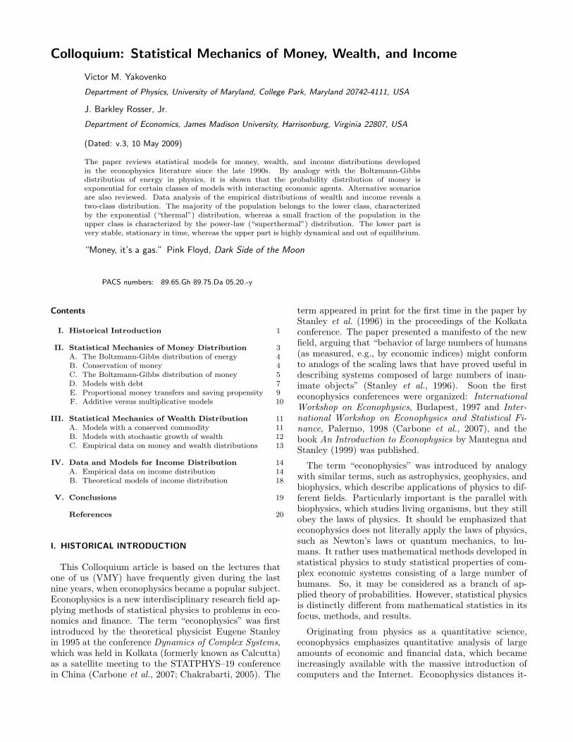
To verify this conjecture, Dragulescu and Yakovenko(2000) performed agent-based computer simulations ofmoney transfers between agents. Initially all agents weregiven the same amount of money, say, $1000. Then, apair of agents (i, j) was randomly selected, the amount∆m was transferred from one agent to another, and theprocess was repeated many times. Time evolution ofthe probability distribution of money P (m) can be seenin computer animation videos by Chen and Yakovenko(2007) and by Wright (2007). After a transitory pe-riod, money distribution converges to the stationary formshown in Fig. 1. As expected, the distribution is very wellfitted by the exponential function (7).

Several different rules for ∆m were considered byDragulescu and Yakovenko (2000). In one model, thetransferred amount was fixed to a constant ∆m = $1.Economically, it means that all agents were selling theirproducts for the same price ∆m = $1. Computer ani-mation (Chen and Yakovenko, 2007) shows that the ini-tial distribution of money first broadens to a symmet-ric Gaussian curve, characteristic for a diffusion pro-cess. Then, the distribution starts to pile up aroundthe m = 0 state, which acts as the impenetrable bound-ary, because of the imposed condition m ≥ 0. As a re-sult, P (m) becomes skewed (asymmetric) and eventu-ally reaches the stationary exponential shape, as shownin Fig. 1. The boundary at m = 0 is analogous tothe ground state energy in statistical physics. Withoutthis boundary condition, the probability distribution ofmoney would not reach a stationary state. Computeranimations (Chen and Yakovenko, 2007; Wright, 2007)also show how the entropy of money distribution, definedas S/N = −

∑

k P (mk) lnP (mk), grows from the initialvalue S = 0, where all agents have the same money, tothe maximal value at the statistical equilibrium.

While the model with ∆m = 1 is very simple and in-structive, it is not very realistic, because all prices aretaken to be the same. In another model considered byDragulescu and Yakovenko (2000), ∆m in each trans-action is taken to be a random fraction of the averageamount of money per agent, i.e., ∆m = ν(M/N), whereν is a uniformly distributed random number between 0and 1. The random distribution of ∆m is supposed torepresent the wide variety of prices for different productsin the real economy. It reflects the fact that agents buyand consume many different types of products, some ofthem simple and cheap, some sophisticated and expen-sive. Moreover, different agents like to consume theseproducts in different quantities, so there is a variation ofthe paid amounts ∆m, even when the unit price of thesame product is constant. Computer simulation of thismodel produces exactly the same stationary distribution

4 Because debt is not permitted in this model, we have M = Mb,where Mb is the monetary base (McConnell and Brue, 1996).

0 1000 2000 3000 4000 5000 60000

2

4

6

8

10

12

14

16

18

Money, m

Pro

babi

lity,

P(m

)

N=500, M=5*105, time=4*105.

⟨m⟩, T

0 1000 2000 30000

1

2

3

Money, m

log

P(m

)

FIG. 1 Histogram and points: Stationary probability distri-bution of money P (m) obtained in agent-based computer sim-ulations. Solid curves: Fits to the Boltzmann-Gibbs law (7).Vertical line: The initial distribution of money. [Reproducedfrom Dragulescu and Yakovenko (2000)]

(7), as in the first model. Computer animation for thismodel is also available on the Web page by Chen andYakovenko (2007).

The final distribution is universal despite different rulesfor ∆m. To amplify this point further, Dragulescu andYakovenko (2000) also considered a toy model, where ∆mwas taken to be a random fraction of the average amountof money of the two agents: ∆m = ν(mi + mj)/2. Thismodel produced the same stationary distribution (7) asthe two other models.

The models of pairwise money transfer are attractivein their simplicity, but they represent a rather prim-itive market. Modern economy is dominated by bigfirms, which consist of many agents, so Dragulescu andYakovenko (2000) also studied a model with firms. Oneagent at a time is appointed to become a “firm”. Thefirm borrows capital K from another agent and returnsit with interest hK, hires L agents and pays them wagesω, manufactures Q items of a product, sells them to Qagents at a price p, and receives profit F = pQ−ωL−hK.All of these agents are randomly selected. The param-eters of the model are optimized following a procedurefrom economics textbooks (McConnell and Brue, 1996).The aggregate demand-supply curve for the product istaken in the form p(Q) = v/Qη, where Q is the quantityconsumers would buy at the price p, and η and v are someparameters. The production function of the firm hasthe traditional Cobb-Douglas form: Q(L, K) = LχK1−χ,where χ is a parameter. Then the profit of the firm F ismaximized with respect to K and L. The net result ofthe firm activity is a many-body transfer of money, whichstill satisfies the conservation law. Computer simulationof this model generates the same exponential distribution(7), independently of the model parameters. The reasonsfor the universality of the Boltzmann-Gibbs distribution

7

and its limitations are discussed in Sec. II.F.Well after the paper by Dragulescu and Yakovenko

(2000) appeared, the Italian econophysicists Patriarca etal. (2005) found that similar ideas had been publishedearlier in obscure Italian journals by Eleonora Bennati(1988, 1993). It was proposed to call these models theBennati-Dragulescu-Yakovenko (BDY) game (Garibaldiet al., 2007; Scalas et al., 2006). The Boltzmann distri-bution was independently applied to social sciences bythe physicist Jurgen Mimkes (2000, 2005) using the La-grange principle of maximization with constraints. Theexponential distribution of money was also found by theeconomist Martin Shubik (1999) using a Markov chainapproach to strategic market games. A long time ago,Benoit Mandelbrot (1960, p 83) observed:

“There is a great temptation to consider theexchanges of money which occur in economicinteraction as analogous to the exchanges ofenergy which occur in physical shocks be-tween gas molecules.”

He realized that this process should result in the expo-nential distribution, by analogy with the barometric dis-tribution of density in the atmosphere. However, he dis-carded this idea, because it does not produce the Paretopower law, and proceeded to study the stable Levy distri-butions. Ironically, the actual economic data, discussedin Secs. III.C and IV.A, do show the exponential distri-bution for the majority of the population. Moreover, thedata have a finite variance, so the stable Levy distribu-tions are not applicable because of their infinite variance.

D. Models with debt

Now let us discuss how the results change when debt ispermitted.5 From the standpoint of individual economicagents, debt may be considered as negative money. Whenan agent borrows money from a bank (considered here asa big reservoir of money),6 the cash balance of the agent(positive money) increases, but the agent also acquiresa debt obligation (negative money), so the total balance(net worth) of the agent remains the same. Thus, the actof borrowing money still satisfies a generalized conserva-tion law of the total money (net worth), which is nowdefined as the algebraic sum of positive (cash M) andnegative (debt D) contributions: M − D = Mb. After

5 The ideas presented here are quite similar to those by Soddy(1926).

6 Here we treat the bank as being outside of the system consistingof ordinary agents, because we are interested in money distribu-tion among these agents. The debt of agents is an asset for thebank, and deposits of cash into the bank are liabilities of the bank(McConnell and Brue, 1996). We do not go into these details inorder to keep our presentation simple. For more discussion, seeKeen (2008).

spending some cash in binary transactions (5), the agentstill has the debt obligation (negative money), so the to-tal money balance mi of the agent (net worth) becomesnegative. We see that the boundary condition mi ≥ 0,discussed in Sec. II.B, does not apply when debt is per-mitted, so m = 0 is not the ground state any more. Theconsequence of permitting debt is not a violation of theconservation law (which is still preserved in the gener-alized form for net worth), but a modification of theboundary condition by permitting agents to have neg-ative balances mi < 0 of net worth. A more detaileddiscussion of positive and negative money and the book-keeping accounting from the econophysics point of viewwas presented by the physicist Dieter Braun (2001) andFischer and Braun (2003a,b).

Now we can repeat the simulation described in Sec.II.C without the boundary condition m ≥ 0 by allowingagents to go into debt. When an agent needs to buy aproduct at a price ∆m exceeding his money balance mi,the agent is now permitted to borrow the difference froma bank and, thus, to buy the product. As a result ofthis transaction, the new balance of the agent becomesnegative: m′

i = mi −∆m < 0. Notice that the local con-servation law (5) and (6) is still satisfied, but it involvesnegative values of m. If the simulation is continued fur-ther without any restrictions on the debt of the agents,the probability distribution of money P (m) never stabi-lizes, and the system never reaches a stationary state. Astime goes on, P (m) keeps spreading in a Gaussian man-ner unlimitedly toward m = +∞ and m = −∞. Becauseof the generalized conservation law discussed above, thefirst moment 〈m〉 = Mb/N of the algebraically definedmoney m remains constant. It means that some agentsbecome richer with positive balances m > 0 at the ex-pense of other agents going further into debt with nega-tive balances m < 0, so that M = Mb + D.

Common sense, as well as the experience with the cur-rent financial crisis, tells us that an economic system can-not be stable if unlimited debt is permitted.7 In this case,agents can buy any goods without producing anything inexchange by simply going into unlimited debt. Arguably,the current financial crisis was caused by the enormousdebt accumulation in the system, triggered by sub-primemortgages and financial derivatives based on them. Awidely expressed opinion is that the current crisis is notthe problem of liquidity, i.e., a temporary difficulty incash flow, but the problem of insolvency, i.e., the inher-ent inability of many participants pay back their debts.

Detailed discussion of the current economic situationis not a subject of this paper. Going back to the idealizedmodel of money transfers, one would need to impose somesort of modified boundary conditions in order to preventunlimited growth of debt and to ensure overall stability of

7 In qualitatively agreement with the conclusions by McCauley(2008).

8

0 2000 4000 6000 80000

2

4

6

8

10

12

14

16

18

Money, m

Pro

babi

lity,

P(m

)

N=500, M=5*105, time=4*105.

Model without debt, T=1000

Model with debt, T=1800

FIG. 2 Histograms: Stationary distributions of money withand without debt. The debt is limited to md = 800. Solidcurves: Fits to the Boltzmann-Gibbs laws with the “moneytemperatures” Tm = 1800 and Tm = 1000. [Reproduced fromDragulescu and Yakovenko (2000)]

the system. Dragulescu and Yakovenko (2000) considereda simple model where the maximal debt of each agent islimited to a certain amount md. This means that theboundary condition mi ≥ 0 is now replaced by the con-dition mi ≥ −md for all agents i. Setting interest rateson borrowed money to be zero for simplicity, Dragulescuand Yakovenko (2000) performed computer simulationsof the models described in Sec. II.C with the new bound-ary condition. The results are shown in Fig. 2. Notsurprisingly, the stationary money distribution again hasthe exponential shape, but now with the new boundarycondition at m = −md and the higher money tempera-ture Td = md+Mb/N . By allowing agents to go into debtup to md, we effectively increase the amount of moneyavailable to each agent by md. So, the money tempera-ture, which is equal to the average amount of effectivelyavailable money per agent, increases correspondingly.

Xi, Ding, and Wang (2005) considered another, morerealistic boundary condition, where a constraint is im-posed not on the individual debt of each agent, but onthe total debt of all agents in the system. This is accom-plished via the required reserve ratio R, which is brieflyexplained below (McConnell and Brue, 1996). Banksare required by law to set aside a fraction R of themoney deposited into bank accounts, whereas the re-maining fraction 1 − R can be loaned further. If theinitial amount of money in the system (the money base)is Mb, then, with repeated loans and borrowing, the to-tal amount of positive money available to the agents in-creases to M = Mb/R, where the factor 1/R is calledthe money multiplier (McConnell and Brue, 1996). Thisis how “banks create money”. Where does this extramoney come from? It comes from the increase of the to-tal debt in the system. The maximal total debt is equal

-50 0 50 100 150

0

10

20

30

40

-50 0 50 100 150

0.1

1

10

log

(P(m

)) (

1x

10

-3)

Monetary Wealth,m

Pro

babi

lity,

P(m

) (1x

10-3)

Monetary Wealth,m

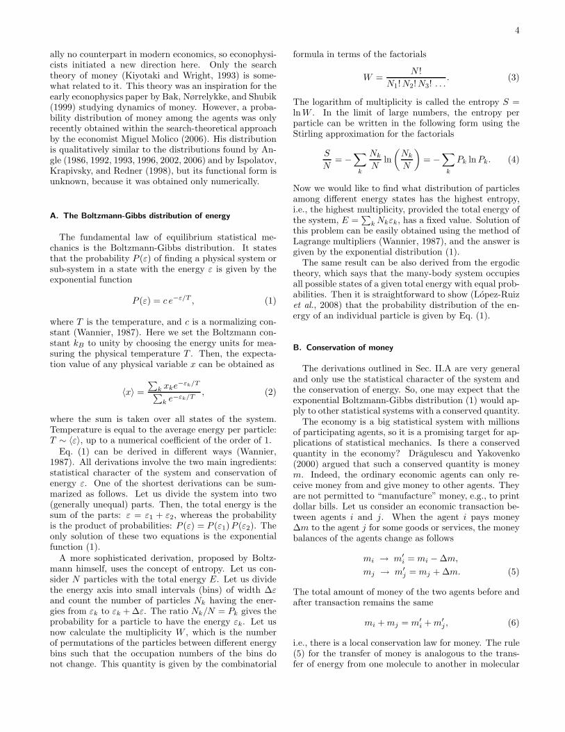
FIG. 3 The stationary distribution of money for the requiredreserve ratio R = 0.8. The distribution is exponential forpositive and negative money with different “temperatures”T+ and T−, as illustrated by the inset on log-linear scale.[Reproduced from Xi, Ding, and Wang (2005)]

to D = Mb/R−Mb and is limited by the factor R. Whenthe debt is maximal, the total amounts of positive, Mb/R,and negative, Mb(1 − R)/R, money circulate among theagents in the system, so there are two constraints in themodel considered by Xi, Ding, and Wang (2005). Thus,we expect to see the exponential distributions of posi-tive and negative money characterized by two differenttemperatures: T+ = Mb/RN and T− = Mb(1 − R)/RN .This is exactly what was found in computer simulationsby Xi, Ding, and Wang (2005), as shown in Fig. 3. Sim-ilar two-sided distributions were also found by Fischerand Braun (2003a).

However, in reality, the reserve requirement is not ef-fective in stabilizing total debt in the system, becauseit applies only to deposits from general public, but notfrom corporations (O′Brien, 2007).8 Moreover, there arealternative instruments of debt, including derivatives andvarious unregulated “financial innovations”. As a re-sult, the total debt is not limited in practice and some-times can reach catastrophic proportions. Here we brieflydiscuss several models with non-stationary debt. Thusfar, we did not consider the interest rates. Dragulescuand Yakovenko (2000) studied a simple model with dif-ferent interest rates for deposits into and loans from abank. Computer simulations found that money distribu-tion among the agents is still exponential, but the moneytemperature slowly changes in time. Depending on thechoice of parameters, the total amount of money in cir-culation either increases or decreases in time. A more

8 Australia does not have reserve requirements, but China activelyuses reserve requirements as a tool of monetary policy.

9

sophisticated macroeconomic model was studied by theeconomist Steve Keen (1995, 2000). He found that oneof the regimes is the debt-induced breakdown, where alleconomic activity stops under the burden of heavy debtand cannot be restarted without a “debt moratorium”.The interest rates were fixed in these models and notadjusted self-consistently. Cockshott and Cottrell (2008)proposed a mechanism, where the interest rates are set tocover probabilistic withdrawals of deposits from a bank.In an agent-based simulation of the model, Cockshott andCottrell (2008) found that money supply first increasesup to a certain limit, and then the economy experiences aspectacular crash under the weight of accumulated debt.Further studies along these lines would be very interest-ing. In the rest of the paper, we review various modelswithout debt proposed in literature.

E. Proportional money transfers and saving propensity

In the models of money transfer discussed in Sec. II.C,the transferred amount ∆m is typically independent ofthe money balances of the agents involved. A differentmodel was introduced in physics literature earlier by Is-polatov, Krapivsky, and Redner (1998) and called themultiplicative asset exchange model. This model also sat-isfies the conservation law, but the transferred amount ofmoney is a fixed fraction γ of the payer’s money in Eq.(5):

∆m = γmi. (8)

The stationary distribution of money in this model, com-pared in Fig. 4 with an exponential function, is similar,but not exactly equal, to the Gamma distribution:

P (m) = c mβ e−m/T . (9)

Eq. (9) differs from Eq. (7) by the power-law prefactormβ . From the Boltzmann kinetic equation (discussedin more detail in Sec. II.F), Ispolatov, Krapivsky, andRedner (1998) derived a formula relating the parametersγ and β in Eqs. (8) and (9):

β = −1 − ln 2/ ln(1 − γ). (10)

When payers spend a relatively small fraction of theirmoney γ < 1/2, Eq. (10) gives β > 0. In this case,the population with low money balances is reduced, andP (0) = 0, as shown in Fig. 4.

The economist Thomas Lux (2005) brought to the at-tention of physicists that essentially the same model,called the inequality process, had been introduced andstudied much earlier by the sociologist John Angle (1986,1992, 1993, 1996, 2002), see also the review by An-gle (2006) for additional references. While Ispolatov,Krapivsky, and Redner (1998) did not give much jus-tification for the proportionality law (8), Angle (1986)connected this rule with the surplus theory of social strat-ification (Engels, 1972), which argues that inequality in

0 1000 2000 3000 4000 50000

2

4

6

8

10

12

14

16

Money, m

Pro

babi

lity,

P(m

)

N=500, M=5*105, α=1/3.

FIG. 4 Histogram: Stationary probability distribution ofmoney in the multiplicative random exchange model (8) forγ = 1/3. Solid curve: The exponential Boltzmann-Gibbs law.[Reproduced from Dragulescu and Yakovenko (2000)]

human society develops when people can produce morethan necessary for minimal subsistence. This additionalwealth (surplus) can be transferred from original pro-ducers to other people, thus generating inequality. Inthe first paper by Angle (1986), the parameter γ wasrandomly distributed, and another parameter δ gave ahigher probability of winning to the agent with the highermoney balance in Eq. (5). However, in the following pa-pers, he simplified the model to a fixed γ (denoted as ω byAngle) and equal probabilities of winning for higher- andlower-balance agents, which makes it completely equiv-alent to the model of Ispolatov, Krapivsky, and Redner(1998). Angle (2002, 2006) also considered a model wheregroups of agents have different values of γ, simulatingthe effect of education and other “human capital”. Allof these models generate a Gamma-like distribution, wellapproximated by Eq. (9).

Another model with an element of proportionality wasproposed by Chakraborti and Chakrabarti (2000).9 Inthis model, the agents set aside (save) some fraction oftheir money λmi, whereas the rest of their money balance(1−λ)mi becomes available for random exchanges. Thus,the rule of exchange (5) becomes

m′i = λmi + ξ(1 − λ)(mi + mj),

m′j = λmj + (1 − ξ)(1 − λ)(mi + mj). (11)

Here the coefficient λ is called the saving propensity, andthe random variable ξ is uniformly distributed between0 and 1. It was pointed out by Angle (2006) that, by

9 This paper originally appeared as a follow-up preprint cond-mat/0004256 on the preprint cond-mat/0001432 by Dragulescuand Yakovenko (2000).

10

the change of notation λ → (1 − γ), Eq. (11) can betransformed to the same form as Eq. (8), if the randomvariable ξ takes only discrete values 0 and 1. Computersimulations by Chakraborti and Chakrabarti (2000) ofthe model (11) found a stationary distribution close tothe Gamma distribution (9). It was shown that the pa-rameter β is related to the saving propensity λ by theformula β = 3λ/(1 − λ) (Patriarca, Chakraborti, andKaski, 2004a,b; Patriarca et al., 2005; Repetowicz, Hut-zler, and Richmond, 2005). For λ 6= 0, agents alwayskeep some money, so their balances never drop to zero,and P (0) = 0, whereas for λ = 0 the distribution be-comes exponential.

In the subsequent papers by the Kolkata school(Chakrabarti, 2005) and related papers, the case of ran-dom saving propensity was studied. In these models,the agents are assigned random parameters λ drawnfrom a uniform distribution between 0 and 1 (Chatter-jee, Chakrabarti, and Manna, 2004). It was found thatthis model produces a power-law tail P (m) ∝ 1/m2 athigh m. The reasons for stability of this law were un-derstood using the Boltzmann kinetic equation (Chat-terjee, Chakrabarti, and Stinchcombe, 2005; Das andYarlagadda, 2005; Repetowicz, Hutzler, and Richmond,2005), but most elegantly in the mean-field theory (Bhat-tacharyya, Chatterjee, and Chakrabarti, 2007; Chatter-jee and Chakrabarti, 2007; Mohanty, 2006). The fat tailoriginates from the agents whose saving propensity isclose to 1, who hoard money and do not give it back(Patriarca, Chakraborti, and Germano, 2006; Patriarcaet al., 2005). A more rigorous mathematical treatmentof the problem was presented by During, Matthes, andToscani (2008); During and Toscani (2007); Matthes andToscani (2008). An interesting matrix formulation of theproblem was presented by Gupta (2006). Relaxation ratein the money transfer models was studied by During,Matthes, and Toscani (2008); Gupta (2008); Patriarca etal. (2007). Dragulescu and Yakovenko (2000) considereda model with taxation, which also has an element of pro-portionality. The Gamma distribution was also studiedfor conservative models within a simple Boltzmann ap-proach by Ferrero (2004) and, using more complicatedrules of exchange motivated by political economy, byScafetta, Picozzi, and West (2004a,b). Independently,the economist Miguel Molico (2006) studied conserva-tive exchange models where agents bargain over pricesin their transactions. He found stationary Gamma-likedistributions of money in numerical simulations of thesemodels.

F. Additive versus multiplicative models

The stationary distribution of money (9) for the mod-els of Sec. II.E is different from the simple exponentialformula (7) found for the models of Sec. II.C. The originof this difference can be understood from the Boltzmannkinetic equation (Lifshitz and Pitaevskii, 1981; Wannier,

1987). This equation describes time evolution of the dis-tribution function P (m) due to pairwise interactions:

dP (m)

dt=

∫∫

{−f[m,m′]→[m−∆,m′+∆]P (m)P (m′) (12)

+f[m−∆,m′+∆]→[m,m′]P (m − ∆)P (m′ + ∆)} dm′ d∆.

Here f[m,m′]→[m−∆,m′+∆] is the probability of transfer-ring money ∆ from an agent with money m to an agentwith money m′ per unit time. This probability, multi-plied by the occupation numbers P (m) and P (m′), givesthe rate of transitions from the state [m, m′] to the state[m−∆, m′ + ∆]. The first term in Eq. (12) gives the de-population rate of the state m. The second term in Eq.(12) describes the reversed process, where the occupationnumber P (m) increases. When the two terms are equal,the direct and reversed transitions cancel each other sta-tistically, and the probability distribution is stationary:dP (m)/dt = 0. This is the principle of detailed balance.

In physics, the fundamental microscopic equations ofmotion obey the time-reversal symmetry. This meansthat the probabilities of the direct and reversed processesare exactly equal:

f[m,m′]→[m−∆,m′+∆] = f[m−∆,m′+∆]→[m,m′]. (13)

When Eq. (13) is satisfied, the detailed balance condi-tion for Eq. (12) reduces to the equation P (m)P (m′) =P (m − ∆)P (m′ + ∆), because the factors f cancels out.The only solution of this equation is the exponential func-tion P (m) = c exp(−m/Tm), so the Boltzmann-Gibbsdistribution is the stationary solution of the Boltzmannkinetic equation (12). Notice that the transition prob-abilities (13) are determined by the dynamical rules ofthe model, but the equilibrium Boltzmann-Gibbs distri-bution does not depend on the dynamical rules at all.This is the origin of the universality of the Boltzmann-Gibbs distribution. We see that it is possible to find thestationary distribution without knowing details of the dy-namical rules (which are rarely known very well), as longas the symmetry condition (13) is satisfied.

The models considered in Sec. II.C have the time-reversal symmetry. The model with the fixed moneytransfer ∆ has equal probabilities (13) of transferringmoney from an agent with the balance m to an agentwith the balance m′ and vice versa. This is also truewhen ∆ is random, as long as the probability distributionof ∆ is independent of m and m′. Thus, the stationarydistribution P (m) is always exponential in these models.

However, there is no fundamental reason to expectthe time-reversal symmetry in economics, where Eq. (13)may be not valid. In this case, the system may have anon-exponential stationary distribution or no stationarydistribution at all. In the model (8), the time-reversalsymmetry is broken. Indeed, when an agent i gives afixed fraction γ of his money mi to an agent with bal-ance mj , their balances become (1−γ)mi and mj +γmi.If we try to reverse this process and appoint the agent jto be the payer and to give the fraction γ of her money,

11

γ(mj + γmi), to the agent i, the system does not returnto the original configuration [mi, mj]. As emphasized byAngle (2006), the payer pays a deterministic fraction ofhis money, but the receiver receives a random amountfrom a random agent, so their roles are not interchange-able. Because the proportional rule typically violatesthe time-reversal symmetry, the stationary distributionP (m) in multiplicative models is typically not exponen-tial.10 Making the transfer dependent on the money bal-ance of the payer effectively introduces Maxwell’s demoninto the model. Another view on the time-reversal sym-metry in economic dynamics was presented by Ao (2007).

These examples show that the Boltzmann-Gibbs dis-tribution does not necessarily hold for any conservativemodel. However, it is universal in a limited sense. Fora broad class of models that have time-reversal symme-try, the stationary distribution is exponential and doesnot depend on details of a model. Conversely, whenthe time-reversal symmetry is broken, the distributionmay depend on details of a model. The difference be-tween these two classes of models may be rather sub-tle. Deviations from the Boltzmann-Gibbs law may oc-cur only if the transition rates f in Eq. (13) explicitlydepend on the agents’ money m or m′ in an asymmetricmanner. Dragulescu and Yakovenko (2000) performeda computer simulation where the direction of paymentwas randomly fixed in advance for every pair of agents(i, j). In this case, money flows along directed links be-tween the agents: i→ j → k, and the time-reversal sym-metry is strongly violated. This model is closer to thereal economy, where one typically receives money froman employer and pays it to a grocery store. Neverthe-less, the Boltzmann-Gibbs distribution was still found inthis model, because the transition rates f do not explic-itly depend on m and m′ and do not violate Eq. (13).A more general study of money exchange models on di-rected networks was presented by Chatterjee (2009).

In the absence of detailed knowledge of real micro-scopic dynamics of economic exchanges, the semiuniver-sal Boltzmann-Gibbs distribution (7) is a natural start-ing point. Moreover, the assumption of Dragulescu andYakovenko (2000) that agents pay the same prices ∆mfor the same products, independent of their money bal-ances m, seems very appropriate for the modern anony-mous economy, especially for purchases over the Internet.There is no particular empirical evidence for the propor-tional rules (8) or (11). However, the difference betweenthe additive (7) and multiplicative (9) distributions maybe not so crucial after all. From the mathematical pointof view, the difference is in the implementation of theboundary condition at m = 0. In the additive modelsof Sec. II.C, there is a sharp cut-off for P (m) 6= 0 at

10 However, when ∆m is a fraction of the total money mi+mj of thetwo agents, the model is time-reversible and has the exponentialdistribution, as discussed in Sec. II.C.

m = 0. In the multiplicative models of Sec. II.E, the bal-ance of an agent never reaches m = 0, so P (m) vanishesat m → 0 in a power-law manner. But for large m, P (m)decreases exponentially in both models.

By further modifying the rules of money transfer andintroducing more parameters in the models, one can ob-tain even more complicated distributions (Saif and Gade,2007; Scafetta and West, 2007). However, one can ar-gue that parsimony is the virtue of a good mathematicalmodel, not the abundance of additional assumptions andparameters, whose correspondence to reality is hard toverify.

III. STATISTICAL MECHANICS OF WEALTH

DISTRIBUTION

In the econophysics literature on exchange models, theterms “money” and “wealth” are often used interchange-ably. However, economists emphasize the difference be-tween these two concepts. In this section, we review themodels of wealth distribution, as opposed to money dis-tribution.

A. Models with a conserved commodity

What is the difference between money and wealth?Dragulescu and Yakovenko (2000) argued that wealth wi

is equal to money mi plus the other property that anagent i has. The latter may include durable materialproperty, such as houses and cars, and financial instru-ments, such as stocks, bonds, and options. Money (papercash, bank accounts) is generally liquid and countable.However, the other property is not immediately liquidand has to be sold first (converted into money) to beused for other purchases. In order to estimate the mon-etary value of property, one needs to know its price p.In the simplest model, let us consider just one type ofproperty, say, stocks s. Then the wealth of an agent i isgiven by the formula

wi = mi + p si. (14)

It is assumed that the price p is common for all agentsand is established by some kind of market process, suchas an auction, and may change in time.

It is reasonable to start with a model where boththe total money M =

∑

i mi and the total stockS =

∑

i si are conserved (Ausloos and Pekalski, 2007;Chakraborti, Pradhan, and Chakrabarti, 2001; Chat-terjee and Chakrabarti, 2006). The agents pay moneyto buy stock and sell stock to get money, and so on.Although M and S are conserved, the total wealthW =

∑

i wi is generally not conserved (Chatterjee andChakrabarti, 2006), because of price fluctuation in Eq.(14). This is an important difference from the moneytransfers models of Sec. II. The wealth wi of an agent i,not participating in any transactions, may change when

12

transactions between other agents establish a new pricep. Moreover, the wealth wi of an agent i does notchange after a transaction with an agent j. Indeed, inexchange for paying money ∆m, the agent i receives thestock ∆s = ∆m/p, so her total wealth (14) remains thesame. Theoretically, the agent can instantaneously sellthe stock back at the same price and recover the moneypaid. If the price p never changes, then the wealth wi ofeach agent remains constant, despite transfers of moneyand stock between agents.

We see that redistribution of wealth in this model isdirectly related to price fluctuations. A mathematicalmodel of this process was studied by Silver, Slud, andTakamoto (2002). In this model, the agents randomlychange preferences for the fraction of their wealth in-vested in stocks. As a result, some agents offer stockfor sale and some want to buy it. The price p is deter-mined from the market-clearing auction matching supplyand demand. Silver, Slud, and Takamoto (2002) demon-strated in computer simulations and proved analyticallyusing the theory of Markov processes that the stationarydistribution P (w) of wealth w in this model is given bythe Gamma distribution, as in Eq. (9). Various modifica-tions of this model considered by Lux (2005), such as in-troducing monopolistic coalitions, do not change this re-sult significantly, which shows robustness of the Gammadistribution. For models with a conserved commodity,Chatterjee and Chakrabarti (2006) found the Gammadistribution for a fixed saving propensity and a powerlaw tail for a distributed saving propensity.

Another model with conserved money and stock wasstudied by Raberto et al. (2003) for an artificial stockmarket, where traders follow different investment strate-gies: random, momentum, contrarian, and fundamen-talist. Wealth distribution in the model with randomtraders was found have a power-law tail P (w) ∼ 1/w2

for large w. However, unlike in most other simulation,where all agents initially have equal balances, here theinitial money and stock balances of the agents were ran-domly populated according to a power law with the sameexponent. This raises the question whether the observedpower-law distribution of wealth is an artifact of the ini-tial conditions, because equilibration of the upper tailmay take a very long simulation time.

B. Models with stochastic growth of wealth

Although the total wealth W is not exactly conservedin the models considered in Sec. III.A, nevertheless W re-mains constant on average, because the total money Mand stock S are conserved. A different model for wealthdistribution was proposed by Bouchaud and Mezard(2000). In this model, time evolution of the wealth wi ofan agent i is given by the stochastic differential equation

dwi

dt= ηi(t)wi +

∑

j( 6=i)

Jijwj −∑

j( 6=i)

Jjiwi, (15)

where ηi(t) is a Gaussian random variable with the mean〈η〉 and the variance 2σ2. This variable represents growthor loss of wealth of an agent due to investment in stockmarket. The last two terms describe transfer of wealthbetween different agents, which is taken to be propor-tional to the wealth of the payers with the coefficients Jij .So, the model (15) is multiplicative and invariant underthe scale transformation wi → Zwi. For simplicity, theexchange fractions are taken to be the same for all agents:Jij = J/N for all i 6= j, where N is the total number ofagents. In this case, the last two terms in Eq. (15) canbe written as J(〈w〉 − wi), where 〈w〉 =

∑

i wi/N is theaverage wealth per agent. This case represents a “mean-field” model, where all agents feel the same environment.It can be easily shown that the average wealth increases

in time as 〈w〉t = 〈w〉0e(〈η〉+σ2)t. Then, it makes more

sense to consider the relative wealth wi = wi/〈w〉t. Eq.(15) for this variable becomes

dwi

dt= (ηi(t) − 〈η〉 − σ2) wi + J(1 − wi). (16)

The probability distribution P (w, t) for the stochasticdifferential equation (16) is governed by the Fokker-Planck equation

∂P

∂t=

∂[J(w − 1) + σ2w]P

∂w+ σ2 ∂

∂w

(

w∂(wP )

∂w

)

. (17)

The stationary solution (∂P/∂t = 0) of this equation isgiven by the following formula

P (w) = ce−J/σ2w

w2+J/σ2. (18)

The distribution (18) is quite different from theBoltzmann-Gibbs (7) and Gamma (9) distributions. Eq.(18) has a power-law tail at large w and a sharp cutoff atsmall w. Eq. (15) is a version of the generalized Lotka-Volterra model, and the stationary distribution (18) wasalso obtained by Solomon and Richmond (2001, 2002).The model was generalized to include negative wealth byHuang (2004).

Bouchaud and Mezard (2000) used the mean-field ap-proach. A similar result was found for a model withpairwise interaction between agents by Slanina (2004).In his model, wealth is transferred between the agentsfollowing the proportional rule (8), but, in addition, thewealth of the agents increases by the factor 1 + ζ in eachtransaction. This factor is supposed to reflect creationof wealth in economic interactions. Because the totalwealth in the system increases, it makes sense to considerthe distribution of relative wealth P (w). In the limit ofcontinuous trading, Slanina (2004) found the same sta-tionary distribution (18). This result was reproducedusing a mathematically more involved treatment of thismodel by Cordier, Pareschi, and Toscani (2005); Pareschiand Toscani (2006). Numerical simulations of the mod-els with stochastic noise η by Scafetta, Picozzi, and West

13

(2004a,b) also found a power law tail for large w. Equiv-alence between the models with pairwise exchange andexchange with a reservoir was discussed by Basu and Mo-hanty (2008).

Let us contrast the models discussed in Secs. III.A andIII.B. In the former case, where money and commodityare conserved, and wealth does not grow, the distribu-tion of wealth is given by the Gamma distribution withthe exponential tail for large w. In the latter models,wealth grows in time exponentially, and the distributionof relative wealth has a power law tail for large w. Theseresults suggest that the presence of a power-law tail isa nonequilibrium effect that requires constant growth orinflation of the economy, but disappears for a closed sys-tem with conservation laws.

The discussed models were reviewed by Chatterjeeand Chakrabarti (2007); Richmond, Hutzler, Coelho,and Repetowicz (2006); Richmond, Repetowicz, Hutzler,and Coelho (2006); Yakovenko (2009) and in the pop-ular article by Hayes (2002). Because of lack of space,we omit discussion of models with wealth condensation(Bouchaud and Mezard, 2000; Braun, 2006; Burda etal., 2002; Ispolatov, Krapivsky, and Redner, 1998; Pi-anegonda et al., 2003), where a few agents accumulate afinite fraction of the total wealth, and studies of wealthdistribution on complex networks (Coelho et al., 2005; DiMatteo, Aste, and Hyde, 2004; Hu et al., 2006, 2007; Igle-sias et al., 2003). So far, we discussed the models withlong-range interaction, where any agent can exchangemoney and wealth with any other agent. A local model,where agents trade only with the nearest neighbors, wasstudied by Bak, Nørrelykke, and Shubik (1999).

C. Empirical data on money and wealth distributions

It would be very interesting to compare theoretical re-sults for money and wealth distributions in various mod-els with empirical data. Unfortunately, such empiricaldata are difficult to find. Unlike income, which is dis-cussed in Sec. IV, wealth is not routinely reported bythe majority of individuals to the government. However,in some countries, when a person dies, all assets mustbe reported for the purpose of inheritance tax. So, inprinciple, there exist good statistics of wealth distribu-tion among dead people, which, of course, is differentfrom the wealth distribution among living people. Usingan adjustment procedure based on the age, gender, andother characteristics of the deceased, the UK tax agency,the Inland Revenue, reconstructed the wealth distribu-tion of the whole population of the UK (Her MajestyRevenue and Customs, 2003). Fig. 5 shows the UK datafor 1996 reproduced from Dragulescu and Yakovenko(2001b). The figure shows the cumulative probabilityC(w) =

∫ ∞

w P (w′) dw′ as a function of the personal netwealth w, which is composed of assets (cash, stocks, prop-erty, household goods, etc.) and liabilities (mortgagesand other debts). Because statistical data are usually

10 100 10000.01%

0.1%

1%

10%

100%

Total net capital (wealth), kpounds

Cum

ulat

ive

perc

ent o

f peo

ple

United Kingdom, IR data for 1996

Pareto

Boltzmann−Gibbs

0 20 40 60 80 10010%

100%

Total net capital, kpounds

FIG. 5 Cumulative probability distribution of net wealth inthe UK shown on log-log (main panel) and log-linear (inset)scales. Points represent the data from the Inland Revenue,and solid lines are fits to the exponential (Boltzmann-Gibbs)and power (Pareto) laws. [Reproduced from Dragulescu andYakovenko (2001b)]

reported at non-uniform intervals of w, it is more practi-cal to plot the cumulative probability distribution C(w)rather than its derivative, the probability density P (w).Fortunately, when P (w) is an exponential or a power-lawfunction, then C(w) is also an exponential or a power-lawfunction.

The main panel in Fig. 5 shows a plot of C(w) on thelog-log scale, where a straight line represents a power-law dependence. The figure shows that the distribu-tion follows a power law C(w) ∝ 1/wα with the expo-nent α = 1.9 for the wealth greater than about 100 k£.The inset in Fig. 5 shows the same data on the log-linear scale, where a straight line represents an expo-nential dependence. We observe that, below 100 k£,the data are well fitted by the exponential distributionC(w) ∝ exp(−w/Tw) with the effective “wealth temper-ature” Tw = 60 k£ (which corresponds to the medianwealth of 41 k£). So, the distribution of wealth is char-acterized by the Pareto power law in the upper tail of thedistribution and the exponential Boltzmann-Gibbs law inthe lower part of the distribution for the great majority(about 90%) of the population. Similar results are foundfor the distribution of income, as discussed in Sec. IV.One may speculate that wealth distribution in the lowerpart is dominated by distribution of money, because thecorresponding people do not have other significant assets(Levy and Levy, 2003), so the results of Sec. II give theBoltzmann-Gibbs law. On the other hand, the uppertail of wealth distribution is dominated by investmentassess (Levy and Levy, 2003), where the results of Sec.III.B give the Pareto law. The power law was studied bymany researchers (Klass et al., 2007; Levy, 2003; Levyand Levy, 2003; Sinha, 2006) for the upper-tail data,such as the Forbes list of 400 richest people. On the

14

other hand, statistical surveys of the population, such asthe Survey of Consumer Finance (Diaz-Gimenez et al.,1997) and the Panel Study of Income Dynamics (PSID),give more information about the lower part of the wealthdistribution. Curiously, Abul-Magd (2002) found thatthe wealth distribution in the ancient Egypt was consis-tent with Eq. (18). Hegyi et al. (2007) found a power-lawtail for the wealth distribution of aristocratic families inmedieval Hungary.

For direct comparison with the results of Sec. II, itwould be very interesting to find data on the distribu-tion of money, as opposed to the distribution of wealth.Making a reasonable assumption that most people keepmost of their money in banks, one can approximate thedistribution of money by the distribution of balances onbank accounts. (Balances on all types of bank accounts,such as checking, saving, and money manager, associatedwith the same person should be added up.) Despite im-perfections (people may have accounts in different banksor not keep all their money in banks), the distributionof balances on bank accounts would give valuable infor-mation about the distribution of money. The data fora big enough bank would be representative of the distri-bution in the whole economy. Unfortunately, it has notbeen possible to obtain such data thus far, even thoughit would be completely anonymous and not compromiseprivacy of bank clients.

The data on the distribution of bank accounts balanceswould be useful, e.g., to the Federal Deposits InsuranceCompany (FDIC) of the USA. This government agencyinsures bank deposits of customers up to a certain max-imal balance. In order to estimate its exposure and thechange in exposure due to a possible increase of the limit,FDIC would need to know the probability distribution ofbalances on bank accounts. It is quite possible FDICmay already have such data.

Measuring the probability distribution of money wouldbe also very useful for determining how much peoplecan, in principle, spend on purchases (without going intodebt). This is different from the distribution of wealth,where the property component, such as a house, a car,or retirement investment, is effectively locked up and, inmost cases, is not easily available for consumer spending.Thus, although wealth distribution may reflect the dis-tribution of economic power, the distribution of moneyis more relevant for immediate consumption.

IV. DATA AND MODELS FOR INCOME DISTRIBUTION

In contrast to money and wealth distributions, a lotmore empirical data are available for the distribution ofincome r from tax agencies and population surveys. Inthis section, we first present empirical data on incomedistribution and then discuss theoretical models.

1 10 100 10000.1%

1%

10%

100%

Adjusted Gross Income, k$

Cum

ulat

ive

perc

ent o

f ret

urns

United States, IRS data for 1997

Pareto

Boltzmann−Gibbs

0 20 40 60 80 100

10%

100%

AGI, k$

FIG. 6 Cumulative probability distribution of tax returns forUSA in 1997 shown on log-log (main panel) and log-linear(inset) scales. Points represent the Internal Revenue Servicedata, and solid lines are fits to the exponential and power-law functions. [Reproduced from Dragulescu and Yakovenko(2003)]

A. Empirical data on income distribution

Empirical studies of income distribution have a longhistory in the economic literature.11 Many articles onthis subject appear in the journal Review of Income andWealth, published on behalf of the International Asso-ciation for Research in Income and Wealth. Followingthe work by Pareto (1897), much attention was focusedon the power-law upper tail of income distribution andless on the lower part. In contrast to more complicatedfunctions discussed in the economic literature (Atkin-son and Bourguignon, 2000; Champernowne and Cow-ell, 1998; Kakwani, 1980), Dragulescu and Yakovenko(2001a) demonstrated that the lower part of income dis-tribution can be well fitted with the simple exponentialfunction P (r) = c exp(−r/Tr), which is characterized byjust one parameter, the “income temperature” Tr. ThenDragulescu and Yakovenko (2001b, 2003) showed thatthe whole income distribution can be fitted by an expo-nential function in the lower part and a power-law func-tion in the upper part, as shown in Fig. 6. The straightline on the log-linear scale in the inset of Fig. 6 demon-strates the exponential Boltzmann-Gibbs law, and thestraight line on the log-log scale in the main panel illus-trates the Pareto power law. The fact that income distri-bution consists of two distinct parts reveals the two-classstructure of the American society (Silva and Yakovenko,2005; Yakovenko and Silva, 2005). Coexistence of the ex-ponential and power-law distributions is also known in

11 See, for example, Atkinson and Bourguignon (2000); Atkinsonand Piketty (2007); Champernowne and Cowell (1998); Kakwani(1980); Piketty and Saez (2003).

15

0.1 1 10 1000.01%

0.1%

1%

10%

100%

1983, 19.35 k$1984, 20.27 k$1985, 21.15 k$1986, 22.28 k$1987, 24.13 k$1988, 25.35 k$1989, 26.38 k$

1990, 27.06 k$1991, 27.70 k$1992, 28.63 k$1993, 29.31 k$1994, 30.23 k$1995, 31.71 k$1996, 32.99 k$1997, 34.63 k$1998, 36.33 k$1999, 38.00 k$2000, 39.76 k$2001, 40.17 k$

Cum

ulat

ive

perc

ent o

f ret

urns

Rescaled adjusted gross income

4.017 40.17 401.70 4017

0.01%

0.1%

1%

10%

100%

Adjusted gross income in 2001 dollars, k$

100%

10% Boltzmann−Gibbs

Pareto

1980’s

1990’s

FIG. 7 Cumulative probability distribution of tax returnsplotted on log-log scale versus r/Tr (the annual income r nor-malized by the average income Tr in the exponential part ofthe distribution). The IRS data points are for 1983–2001,and the columns of numbers give the values of Tr for thecorresponding years. [Reproduced from Silva and Yakovenko(2005)]

plasma physics and astrophysics, where they are calledthe “thermal” and “superthermal” parts (Collier, 2004;Desai et al., 2003; Hasegawa et al., 1985). The boundarybetween the lower and upper classes can be defined asthe intersection point of the exponential and power-lawfits in Fig. 6. For 1997, the annual income separating thetwo classes was about 120 k$. About 3% of the popula-tion belonged to the upper class, and 97% belonged tothe lower class.

Silva and Yakovenko (2005) studied time evolution ofincome distribution in the USA during 1983–2001 usingthe data from the Internal Revenue Service (IRS), thegovernment tax agency. The structure of income dis-tribution was found to be qualitatively the same for allyears, as shown in Fig. 7. The average income in nom-inal dollars has approximately doubled during this timeinterval. So, the horizontal axis in Fig. 7 shows the nor-malized income r/Tr, where the “income temperature”Tr was obtained by fitting of the exponential part of thedistribution for each year. The values of Tr are shownin Fig. 7. The plots for the 1980s and 1990s are shiftedvertically for clarity. We observe that the data points inthe lower-income part of the distribution collapse on thesame exponential curve for all years. This demonstratesthat the shape of the income distribution for the lowerclass is extremely stable and does not change in time, de-spite gradual increase of the average income in nominaldollars. This observation suggests that the lower-classdistribution is in statistical, “thermal” equilibrium.

On the other hand, as Fig. 7 shows, income distribu-tion of the upper class does not rescale and significantlychanges in time. Silva and Yakovenko (2005) found thatthe exponent α of the power law C(r) ∝ 1/rα decreased

0 10 20 30 40 50 60 70 80 90 100%0

10

20

30

40

50

60

70

80

90

100%

Cumulative percent of tax returns

Cum

ulat

ive

perc

ent o

f inc

ome

US, IRS data for 1983 and 2000

1983→

←2000

4%

19%

1980 1985 1990 1995 2000 0

0.5

1

Year

Gini from IRS dataGini=(1+f)/2

FIG. 8 Main panel: Lorenz plots for income distribution in1983 and 2000. The data points are from the IRS (Strudler,Petska, and Petska, 2003), and the theoretical curves rep-resent Eq. (20) with the parameter f deduced from Fig. 7.Inset: The closed circles are the IRS data (Strudler, Petska,and Petska, 2003) for the Gini coefficient G, and the open cir-cles show the theoretical formula G = (1+f)/2. [Reproducedfrom Silva and Yakovenko (2005)]

from 1.8 in 1983 to 1.4 in 2000. This means that the up-per tail became “fatter”. Another useful parameter is thetotal income of the upper class as the fraction f of the to-tal income in the system. The fraction f increased from4% in 1983 to 20% in 2000 (Silva and Yakovenko, 2005).However, in year 2001, α increased and f decreases, in-dicating that the upper tail was reduced after the stockmarket crash at that time. These results indicate thatthe upper tail is highly dynamical and not stationary. Ittends to swell during the stock market boom and shrinkduring the bust. Similar results were found for Japan(Aoyama et al., 2003; Fujiwara et al., 2003; Souma, 2001,2002).

Although relative income inequality within the lowerclass remains stable, the overall income inequality in theUSA has increased significantly as a result of the tremen-dous growth of the income of the upper class. This isillustrated by the Lorenz curve and the Gini coefficientshown in Fig. 8. The Lorenz curve (Kakwani, 1980) is astandard way of representing income distribution in theeconomic literature. It is defined in terms of two coordi-nates x(r) and y(r) depending on a parameter r:

x(r) =

∫ r

0

P (r′) dr′, y(r) =

∫ r

0r′P (r′) dr′

∫ ∞

0 r′P (r′) dr′. (19)

The horizontal coordinate x(r) is the fraction of the pop-ulation with income below r, and the vertical coordinatey(r) is the fraction of the income this population accountsfor. As r changes from 0 to ∞, x and y change from 0 to1 and parametrically define a curve in the (x, y) plane.

Fig. 8 shows the data points for the Lorenz curvesin 1983 and 2000, as computed by the IRS (Strudler,

16

0%

5%

10%

15%

20%

25%

30%

Years

Per

cent

age

of to

tal i

ncom

e in

tail

1985 1990 1995 2000 20050

10

20

30

40

50

60

Ave

rage

inco

me

in k

$

Tr

⟨ r ⟩

f

FIG. 9 Historical evolution of the parameters 〈r〉, Tr, and thefraction of income f going to the upper tail, as defined in Eq.(21). [Reproduced from Banerjee (2008)]

Petska, and Petska, 2003). Dragulescu and Yakovenko(2001a) analytically derived the Lorenz curve formulay = x + (1 − x) ln(1 − x) for a purely exponential dis-tribution P (r) = c exp(−r/Tr). This formula is shownby the upper curve in Fig. 8 and describes the 1983 datareasonably well. However, for year 2000, it is essentialto take into account the fraction f of income in the up-per tail, which modifies for the Lorenz formula as follows(Dragulescu and Yakovenko, 2003; Silva and Yakovenko,2005; Yakovenko and Silva, 2005)

y = (1 − f)[x + (1 − x) ln(1 − x)] + f Θ(x − 1). (20)

The last term in Eq. (20) represent the vertical jump ofthe Lorenz curve at x = 1, where a very small percentageof population in the upper class accounts for a substantialfraction f of the total income. The lower curve in Fig. 8shows that Eq. (20) fits the 2000 data very well.

The deviation of the Lorenz curve from the straightdiagonal line in Fig. 8 is a certain measure of incomeinequality. Indeed, if everybody had the same income,the Lorenz curve would be the diagonal line, because thefraction of income would be proportional to the fractionof the population. The standard measure of income in-equality is the Gini coefficient 0 ≤ G ≤ 1, which is de-fined as the area between the Lorenz curve and the di-agonal line, divided by the area of the triangle beneaththe diagonal line (Kakwani, 1980). Time evolution of theGini coefficient, as computed by the IRS (Strudler, Pet-ska, and Petska, 2003), is shown in the inset of Fig. 8.Dragulescu and Yakovenko (2001a) derived analyticallythe result that G = 1/2 for a purely exponential distribu-tion. In the first approximation, the values of G shownin the inset of Fig. 8 are indeed close to the theoreticalvalue 1/2. If we take into account the upper tail usingEq. (20), the formula for the Gini coefficient becomesG = (1 + f)/2 (Silva and Yakovenko, 2005). The insetin Fig. 8 shows that this formula gives a very good fit tothe IRS data for the 1990s using the values of f deducedfrom Fig. 7. The values G < 1/2 in the 1980s cannot be

0 10 20 30 40 50 60 70 80 90 100 110 1200%

1%

2%

3%

4%

5%

6%

Annual family income, k$

Pro

babi

lity

United States, Bureau of Census data for 1996

FIG. 10 Histogram: Probability distribution of family in-come for families with two adults (US Census Bureau data).Solid line: Fit to Eq. (22). [Reproduced from Dragulescu andYakovenko (2001a).]

captured by this formula, because the Lorenz data pointsare slightly above the theoretical curve for 1983 in Fig.8. Overall, we observe that income inequality has beenincreasing for the last 20 years, because of swelling of thePareto tail, but decreased in 2001 after the stock marketcrash.

It is easy to show that the parameter f in Eq. (20) andin Fig. 8 is given by the following formula

f =〈r〉 − Tr

〈r〉, (21)

where 〈r〉 is the average income of the whole population,and the “temperature” Tr is the average income in theexponential part of the distribution. Eq. (21) gives awell-defined measure of the deviation of the actual in-come distribution from the exponential one and, thus, ofthe “fatness” of the upper tail. Fig. 9 shows historicalevolution of the parameters 〈r〉, Tr, and f given by Eq.(21).12 We observe that Tr has been increasing, essen-tially, monotonously (most of this increase is inflation).In contrast, 〈r〉 had sharp peaks in 2000 and 2006 coin-ciding with the speculative bubbles in financial markets.The fraction f , which characterizes income inequality,has been increasing for the last 20 years and reachedmaxima of 20% in the years 2000 and 2006 with a sharpdrop in between. We conclude that the speculative bub-bles greatly increase the fraction of income going to theupper tail, but do not change income distribution of thelower class. When the bubbles inevitably collapse, in-come inequality reduces.

12 A similar plot was constructed by Silva and Yakovenko (2005)for an earlier historical dataset.

17

0 20 40 60 80 1000

20

40

60

80

100

Labor income of one earner, k$

Labo

r in

com

e of

ano

ther

ear

ner,

k$

PSID data for families, 1999

FIG. 11 Scatter plot of the spouses’ incomes (r1, r2) and(r2, r1) based on the data from the Panel Study of Income Dy-namics (PSID). [Reproduced from Dragulescu and Yakovenko(2003)]

Thus far, we discussed the distribution of individualincome. An interesting related question is the distribu-tion P2(r) of family income r = r1 + r2, where r1 and r2

are the incomes of spouses. If the individual incomes aredistributed exponentially P (r) ∝ exp(−r/Tr), then

P2(r) =

∫ r

0

dr′P (r′)P (r − r′) = c r exp(−r/Tr), (22)

where c is a normalization constant. Fig. 10 shows thatEq. (22) is in good agreement with the family income dis-tribution data from the US Census Bureau (Dragulescuand Yakovenko, 2001a). In Eq. (22), we assumed thatincomes of spouses are uncorrelated. This simple ap-proximation is indeed supported by the scatter plot ofincomes of spouses shown in Fig. 11. Each family is rep-resented in this plot by two points (r1, r2) and (r2, r1) forsymmetry. We observe that the density of points is ap-proximately constant along the lines of constant familyincome r1 + r2 = const, which indicates that incomes ofspouses are approximately uncorrelated. There is no sig-nificant clustering of points along the diagonal r1 = r2,i.e., no strong positive correlation of spouses’ incomes.

The Gini coefficient for the family income distribu-tion (22) was analytically calculated by Dragulescu andYakovenko (2001a) as G = 3/8 = 37.5%. Fig. 12shows the Lorenz quintiles and the Gini coefficient for1947–1994 plotted from the US Census Bureau data(Dragulescu and Yakovenko, 2001a). The solid line, rep-resenting the Lorenz curve calculated from Eq. (22), isin good agreement with the data. The systematic de-viation for the top 5% of earners results from the up-per tail, which has a less pronounced effect on familyincome than on individual income, because of incomeaveraging in the family. The Gini coefficient, shown in

0 10 20 30 40 50 60 70 80 90 100%0

10

20

30

40

50

60

70

80

90

100%

Cum

ulat

ive

perc

ent o

f fam

ily in

com

e

United States, Bureau of Census data for 1947−1994

Cumulative percent of families

1950 1960 1970 1980 19900

0.2

0.375

0.6

0.8

1

Year

Gini coefficient ≈ 38

FIG. 12 Main panel: Lorenz plot for family income calculatedfrom Eq. (22), compared with the US Census data points.Inset: The US Census data points for the Gini coefficientfor families, compared with the theoretically calculated value3/8=37.5%. [Reproduced from Dragulescu and Yakovenko(2001a)]

the inset of Fig. 12, is close to the calculated value of37.5%. Notice that income distribution is very stablefor a long period of time, which was also recognized bythe economists (Levy, 1987). Moreover, the average Gfor the developed capitalist countries of North Americaand western Europe, as determined by the World Bank,is also close to the calculated value 37.5% (Dragulescuand Yakovenko, 2003). However, within this average, na-tions or groups of nations may have quite different Ginicoefficients that persist over time due to specific histori-cal, political, or social circumstances (Rosser and Rosser,2004). The Nordic economies, with their famously redis-tributive welfare states, tend to have G in the mid-20%,while many of the Latin American countries have G over50%, reflecting entrenched social patterns inherited fromthe colonial era.

Income distribution has been examined in econo-physics papers for different countries: Japan (Aoyamaet al., 2003; Ferrero, 2004, 2005; Fujiwara et al., 2003;Nirei and Souma, 2007; Souma, 2001, 2002; Souma andNirei, 2005), Germany (Clementi and Gallegati, 2005a;Clementi, Gallegati, and Kaniadakis, 2007), the UK(Clementi and Gallegati, 2005a; Clementi, Gallegati, andKaniadakis, 2007; Ferrero, 2004, 2005; Richmond, Hut-zler, Coelho, and Repetowicz, 2006), Italy (Clementi,Di Matteo, and Gallegati, 2006; Clementi and Galle-gati, 2005b; Clementi, Gallegati, and Kaniadakis, 2007),the USA (Clementi and Gallegati, 2005a; Rawlings etal., 2004), India (Sinha, 2006), Australia (Banerjee,Yakovenko, and Di Matteo, 2006; Clementi, Di Matteo,and Gallegati, 2006; Di Matteo, Aste, and Hyde, 2004),and New Zealand (Ferrero, 2004, 2005). The distribu-tions are qualitatively similar to the results presented in

18

this section. The upper tail follows a power law andcomprises a small fraction of population. To fit the lowerpart of the distribution, different papers used the expo-nential, Gamma, and log-normal distributions. Unfortu-nately, income distribution is often reported by statisti-cal agencies for households, so it is difficult to differen-tiate between one-earner and two-earner income distri-butions. Some papers used interpolating functions withdifferent asymptotic behavior for low and high incomes,such as the Tsallis function (Ferrero, 2005) and the Ka-niadakis function (Clementi, Gallegati, and Kaniadakis,2007). However, the transition between the lower and up-per classes is not smooth for the US data shown in Figs. 6and 7, so such functions would not be useful in this case.The special case is income distribution in Argentina dur-ing the economic crisis, which shows a time-dependentbimodal shape with two peaks (Ferrero, 2005).

B. Theoretical models of income distribution

Having examined the empirical data on income distri-bution, let us now discuss theoretical models. Incomeri is the influx of money per unit time to an agent i.If the money balance mi is analogous to energy, thenthe income ri would be analogous to power, which is theenergy flux per unit time. So, one should conceptuallydistinguish between the distributions of money and in-come. While money is regularly transferred from oneagent to another in pairwise transactions, it is not typi-cal for agents to trade portions of their income. Never-theless, indirect transfer of income may occur when oneemployee is promoted and another demoted while the to-tal annual budget is fixed, or when one company gets acontract whereas another one loses it, etc. A reasonableapproach, which has a long tradition in the economicliterature (Champernowne, 1953; Gibrat, 1931; Kalecki,1945), is to treat individual income r as a stochastic pro-cess and study its probability distribution. In general,one can study a Markov process generated by a matrix oftransitions from one income to another. In the case wherethe income r changes by a small amount ∆r over a timeperiod ∆t, the Markov process can be treated as incomediffusion. Then one can apply the general Fokker-Planckequation (Lifshitz and Pitaevskii, 1981) to describe evo-lution in time t of the income distribution function P (r, t)(Silva and Yakovenko, 2005)

∂P

∂t=

∂

∂r

[

AP +∂(BP )

∂r

]

, A = −〈∆r〉

∆t, B =

〈(∆r)2〉

2∆t.

(23)The coefficients A and B in Eq. (23) are determined bythe first and second moments of income changes per unittime. The stationary solution ∂tP = 0 of Eq. (23) obeysthe following equation with the general solution

∂(BP )

∂r= −AP, P (r) =

c

B(r)exp

(

−

∫ r A(r′)

B(r′)dr′

)

.

(24)

For the lower part of the distribution, it is reasonableto assume that ∆r is independent of r, i.e., the changes ofincome are independent of income itself. This process iscalled the additive diffusion (Silva and Yakovenko, 2005).In this case, the coefficients in Eq. (23) are the constantsA0 and B0. Then Eq. (24) gives the exponential dis-tribution P (r) ∝ exp(−r/Tr) with the effective incometemperature Tr = B0/A0.

13 The coincidence of this re-sult with the Boltzmann-Gibbs exponential law (1) and(7) is not accidental. Indeed, instead of considering pair-wise interaction between particles, one can derive Eq. (1)by considering energy transfers between a particle and abig reservoir, as long as the transfer process is “additive”and does not involve a Maxwell-demon-like discrimina-tion (Basu and Mohanty, 2008). So, although moneyand income are different concepts, they may have similardistributions, because they are governed by similar math-ematical principles. It was shown explicitly by Cordier,Pareschi, and Toscani (2005); Dragulescu and Yakovenko(2000); Slanina (2004) that the models of pairwise moneytransfer can be described in a certain limit by the Fokker-Planck equation.

On the other hand, for the upper tail of income dis-tribution, it is reasonable to expect that ∆r ∝ r, i.e.,income changes are proportional to income itself. This isknown as the proportionality principle of Gibrat (1931),and the process is called the multiplicative diffusion(Silva and Yakovenko, 2005). In this case, A = ar andB = br2, and Eq. (24) gives the power-law distributionP (r) ∝ 1/rα+1 with α = 1 + a/b.

Generally, the lower-class income comes from wagesand salaries, where the additive process is appropriate,whereas the upper-class income comes from bonuses,investments, and capital gains, calculated in percent-ages, where the multiplicative process applies (Milakovic,2005). However, the additive and multiplicative pro-cesses may coexist. An employee may receive a cost-of-living raise calculated in percentages (the multiplicativeprocess) and a merit raise calculated in dollars (the addi-tive process). Assuming that these processes are uncorre-lated, we have A = A0+ar and B = B0+br2 = b(r2

0+r2),where r2

0 = B0/b. Substituting these expressions into Eq.(24), we find

P (r) = ce−(r0/Tr) arctan(r/r0)

[1 + (r/r0)2]1+a/2b. (25)

The distribution (25) interpolates between the exponen-tial law for low r and the power law for high r, becauseeither the additive or the multiplicative process domi-nates in the corresponding limit. The crossover betweenthe two regimes takes place at r = r0, where the ad-ditive and multiplicative contributions to B are equal.

13 Notice that a meaningful stationary solution (24) requires thatA > 0, i.e., 〈∆r〉 < 0.

19

10−2

10−1

100

101

102

10−5

10−4

10−3

10−2

10−1

100

Annual Income/T

Cum

ulat

ive

Dis

trib

utio

n F

unct

ion

2005

1995

FIG. 13 Fits of the IRS data for income distribution usingEq. (25). Plots for different years are shifted vertically forclarity. [Reproduced from Banerjee (2008)]

The distribution (25) has three parameters: the “in-come temperature” Tr = A0/B0, the Pareto exponentα = 1 + a/b, and the crossover income r0. It is a mini-mal model that captures the salient features of the em-pirical income distribution. Eq. (25) was obtained byYakovenko (2009), and a more general formula for cor-related additive and multiplicative processes was derivedby Fiaschi and Marsili (2009) for a sophisticated eco-nomic model. Fits of the IRS data using Eq. (25) areshown in Fig. 13 reproduced from Banerjee (2008). Amathematically similar, but more economically orientedmodel was proposed by Nirei and Souma (2007); Soumaand Nirei (2005), where labor income and assets accumu-lation are described by the additive and multiplicativeprocesses correspondingly. A general stochastic processwith additive and multiplicative noise was studied nu-merically by Takayasu et al. (1997), but the stationarydistribution was not derived analytically. A similar pro-cess with discrete time increments was studied by Kesten(1973). Besides economic applications, Eq. (25) may bealso useful for general stochastic processes with additiveand multiplicative components.

To verify the multiplicative and additive hypothesesempirically, it is necessary to have data on income mo-bility, i.e., the income changes ∆r of the same peoplefrom one year to another. The distribution of incomechanges P (∆r|r) conditional on income r is generally notavailable publicly, although it can be reconstructed byresearchers at the tax agencies. Nevertheless, the mul-

tiplicative hypothesis for the upper class was quantita-tively verified by Aoyama et al. (2003); Fujiwara et al.

(2003) for Japan, where such data for the top taxpayersare publicly available.

The power-law distribution is meaningful only whenit is limited to high enough incomes r > r0. If allincomes r from 0 to ∞ follow a purely multiplicativeprocess (A0 = 0 and B0 = 0), then one can changeto a logarithmic variable x = ln(r/r∗) in Eq. (23) andshow that it gives a Gaussian time-dependent distribu-tion Pt(x) ∝ exp(−x2/2σ2t) for x, i.e., the log-normaldistribution for r, also known as the Gibrat distribution(Gibrat, 1931). However, the width of this distributionincreases linearly in time, so the distribution is not sta-tionary. This was pointed out by Kalecki (1945) a longtime ago, but the log-normal distribution is still widelyused for fitting income distribution, despite this funda-mental logical flaw in its justification. In the classic pa-per, Champernowne (1953) showed that a multiplicativeprocess gives a stationary power-law distribution whena boundary condition is imposed at r0 6= 0. Later, thisresult was rediscovered by econophysicists (Levy, 2003;Levy and Solomon, 1996; Sornette and Cont, 1997). Inour Eq. (25), the exponential distribution of the lowerclass effectively provides such a boundary condition forthe power law of the upper class. Notice also that Eq.(25) reduces to Eq. (18) in the limit r0 → 0 with B0 = 0,but A0 6= 0.

There are alternative approaches to income distribu-tion in economic literature. One of them, proposed byLydall (1959), involves social hierarchy. Groups of peo-ple have leaders, which have leaders of the higher order,and so on. The number of people decreases geometri-cally (exponentially) with the increase of the hierarchicallevel. If individual income increases by a certain factor(i.e., multiplicatively) when moving to the next hierar-chical level, then income distribution follows a power law(Lydall, 1959). However, this original argument of Ly-dall can be easily modified to produce the exponentialdistribution. If individual income increases by a certainamount, i.e., income increases linearly with the hierarchi-cal level, then income distribution is exponential. Thelatter process seems to be more realistic for moderateannual incomes below 100 k$. A similar scenario is theBernoulli trials (Feller, 1966), where individuals have aconstant probability of increasing their income by a fixedamount. We see that the deterministic hierarchical mod-els and the stochastic models of additive and multiplica-tive income mobility represent essentially the same ideas.

V. CONCLUSIONS

The “invasion” of physicists into economics and fi-nance at the turn of the millennium is a fascinatingphenomenon. It generated a lively public debate aboutthe role and future perspectives of econophysics, covering

20

both theoretical and empirical issues.14 The econophysi-cist Joseph McCauley proclaimed that “Econophysicswill displace economics in both the universities andboardrooms, simply because what is taught in economicsclasses doesn’t work” (Ball, 2006). Although there issome truth in his arguments (McCauley, 2006), one mayconsider a less radical scenario. Econophysics may be-come a branch of economics, in the same way as gametheory, psychological economics, and now agent-basedmodeling became branches of economics. These brancheshave their own interests, methods, philosophy, and jour-nals. When infusion of new ideas from a different fieldhappens, the main contribution often consists not inanswering old questions, but in raising new questions.Much of the misunderstanding between economists andphysicists happens not because they are getting differentanswers, but because they are answering different ques-tions.

The subject of income and wealth distributions andsocial inequality was very popular at the turn of an-other century and is associated with the names of Pareto,Lorenz, Gini, Gibrat, and Champernowne, among others.Following the work by Pareto, attention of researcherswas primarily focused on the power laws. However, whenphysicists took a fresh look at the empirical data, theyfound a different, exponential law for the lower part ofthe distribution. Demonstration of the ubiquitous na-ture of the exponential distribution for money, wealth,and income is one of the new contributions produced byeconophysics.15 The motivation, of course, came fromthe Boltzmann-Gibbs distribution in physics. Furtherstudies revealed a more detailed picture of the two-classdistribution in a society. Although social classes havebeen known in political economy since Karl Marx, real-ization that they are described by simple mathematicaldistributions is quite new. Very interesting work wasdone by the computer scientist Ian Wright (2005, 2008),who demonstrated emergence of two classes in an agent-based simulation of initially equal agents. This workis further developed in the upcoming book by Cottrell,Cockshott, Michaelson, Wright, and Yakovenko (2009),integrating economics, computer science, and physics.

Econophysics may be also useful for teaching of sta-tistical physics. If nothing else, it helps to clarify thefoundations of statistical physics by applying it to non-traditional objects. Practitioners of statistical physicsknow very well that the major fascinating attraction of

14 See, for example, Anglin (2005); Ball (2006); Carbone et al.

(2007); Gallegati, Keen, Lux, and Ormerod (2006); Keen (2008);Lux (2005, 2009); McCauley (2006); Richmond, Chakrabarti,Chatterjee, and Angle (2006); Rosser (2006, 2008b); Stauffer(2004); Yakovenko (2009).

15 The exponential distribution is also ubiquitous in the probabil-ity distributions of financial returns (Kleinert and Chen, 2007;McCauley and Gunaratne, 2003; Silva, Prange, and Yakovenko,2004) and the growth rates of firms.

this field is the enormous breadth of its applications.

References

Abul-Magd, A. Y., 2002, “Wealth distribution in an ancientEgyptian society,” Physical Review E 66, 057104.

Anderson, P. W., K. J. Arrow, and D. Pines, 1988, Eds.,The Economy as an Evolving Complex System (Addison-Wesley, Reading).

Angle, J., 1986, “The surplus theory of social stratificationand the size distribution of personal wealth,” Social Forces65, 293–326.

Angle, J., 1992, “The inequality process and the distributionof income to blacks and whites,” Journal of MathematicalSociology 17, 77–98.

Angle, J., 1993, “Deriving the size distribution of personalwealth from ‘the rich get richer, the poor get poorer’,”Journal of Mathematical Sociology 18, 27–46.

Angle, J., 1996, “How the Gamma Law of income distributionappears invariant under aggregation,” Journal of Mathe-matical Sociology 21, 325–358.

Angle, J., 2002, “The statistical signature of pervasive com-petition on wage and salary incomes,” Journal of Mathe-matical Sociology 26, 217–270.

Angle, J., 2006, “The Inequality Process as a wealth maxi-mizing process,” Physica A 367, 388–414.

Anglin, P., 2005, “Econophysics of wealth distributions: acomment,” in Chatterjee, Yarlagadda, and Chakrabarti(2005), pp. 229–238.

Ao, P., 2007, “Boltzmann-Gibbs distribution of fortune andbroken time reversible symmetry in econodynamics,” Com-munications in Nonlinear Science and Numerical Simula-tion 12, 619–626.

Aoyama, H., W. Souma, and Y. Fujiwara, 2003, “Growth andfluctuations of personal and company’s income,” Physica A324, 352–358.

Atkinson, A. B., and F. Bourguignon, 2000, Eds., Handbookof Income Distribution (Elsevier, Amsterdam).

Atkinson, A. B., and T. Piketty, 2007, Eds., Top Incomes overthe Twentieth Century (Oxford University Press, Oxford).

Ausloos, M., and A. Pekalski, 2007, “Model of wealth andgoods dynamics in a closed market,” Physica A 373, 560–568.

Bak P., S. F. Nørrelykke, and M. Shubik, 1999, “Dynamics ofmoney,” Physical Review E 60, 2528–2532.

Ball, P., 2002, “The physical modelling of society: a historicalperspective,” Physica A 314, 1–14.

Ball, P., 2004, Critical Mass: How One Thing Leads to An-other (Farrar, Straus and Giroux, New York).

Ball, P., 2006, “Econophysics: Culture Crash,” Nature 441,686–688.

Banerjee, A., 2008, Ph.D. thesis (Department of Physics, Uni-versity of Maryland).

Banerjee, A., V. M. Yakovenko, and T. Di Matteo, 2006, “Astudy of the personal income distribution in Australia,”Physica A 370, 54–59.

Basu, U., and P. K. Mohanty, 2008, “Modeling wealth distri-bution in growing markets,” The European Physical Jour-nal B 65, 585–589.

Bennati, E., 1988, “Un metodo di simulazione statisticaper l’analisi della distribuzione del reddito,” Rivista Inter-nazionale di Scienze Economiche e Commerciali 35, 735–

21

756.Bennati, E., 1993, “Il metodo di Montecarlo nell’analisi eco-

nomica,” Rassegna di Lavori dell’ISCO (Istituto Nazionaleper lo Studio della Congiuntura), Anno X, No. 4, pp. 31–79.

Bhattacharyya, P., A. Chatterjee, and B. K. Chakrabarti,2007, “A common mode of origin of power laws in modelsof market and earthquake,” Physica A 381, 377–382.

Blume, L. E., 1993, “The statistical mechanics of strategicinteraction,” Games and Economic Behavior 5, 387–424.

Boltzmann, L., 1905, Populare Schriften (Barth, Leipzig), p.S.360f.

Boltzmann, L., 2006, Ludwig Boltzmann 1844–1906 (Aus-trian Central Library for Physics, Vienna), ISBN 3-900490-11-2, p. 113.

Bouchaud, J.-P., and M. Mezard, 2000, “Wealth condensationin a simple model of economy,” Physica A 282, 536–545.

Braun, D., 2001, “Assets and liabilities are the momentum ofparticles and antiparticles displayed in Feynman-graphs,”Physica A 290, 491–500.

Braun, D., 2006, “Nonequilibrium thermodynamics of wealthcondensation,” Physica A 369, 714–722.

Burda, Z., D. Johnston, J. Jurkiewicz, M. Kaminski, M. A.Nowak, G. Papp, and I. Zahed, 2002, “Wealth condensationin Pareto macroeconomies,” Physical Review E 65, 026102.

Carbone, A., G. Kaniadakis, and A. M. Scarfone, 2007,“Where do we stand on econophysics?” Physica A 382,xi–xiv.

Chakrabarti, B. K., 2005, “Econophys-Kolkata: a shortstory,” in Chatterjee, Yarlagadda, and Chakrabarti (2005),pp. 225–228.

Chakrabarti, B. K., A. Chakraborti, and A. Chatterjee, 2006,Eds., Econophysics and Sociophysics: Trends and Perspec-tives (Wiley-VCH, Berlin).

Chakraborti A., and B. K. Chakrabarti, 2000, “Statisticalmechanics of money: how saving propensity affects its dis-tribution,” The European Physical Journal B 17, 167–170.

Chakraborti, A., S. Pradhan, and B. K. Chakrabarti, 2001,“A self-organising model of market with single commodity,”Physica A 297, 253–259.

Champernowne, D. G., 1953, “A model of income distribu-tion,” The Economic Journal 63, 318–351.

Champernowne, D. G., and F. A. Cowell, 1998, EconomicInequality and Income Distribution (Cambridge UniversityPress, Cambridge).

Chatterjee, A., 2009 “Kinetic models for wealth exchange ondirected networks,” The European Physical Journal B 67,593–598.

Chatterjee, A., and B. K. Chakrabarti, 2006, “Kinetic marketmodels with single commodity having price fluctuations,”The European Physical Journal B 54, 399–404.

Chatterjee, A., and B. K. Chakrabarti, 2007, “Kinetic ex-change models for income and wealth distributions,” TheEuropean Physical Journal B 60, 135–149.

Chatterjee, A., B. K. Chakrabarti, and S. S. Manna, 2004,“Pareto law in a kinetic model of market with random sav-ing propensity,” Physica A 335, 155-163.

Chatterjee, A., B. K. Chakrabarti, and R. B. Stinchcombe,2005, “Master equation for a kinetic model of a tradingmarket and its analytic solution,” Physical Review E 72,026126.

Chatterjee, A., S. Yarlagadda, and B. K. Chakrabarti, 2005,Eds., Econophysics of Wealth Distributions (Springer, Mi-lan).

Chen, J., and V. M. Yakovenko, 2007, Computer animation

videos of money-transfer models, http://www2.physics.

umd.edu/~yakovenk/econophysics/animation.html.Clementi, F., T. Di Matteo, and M. Gallegati, 2006, “The

power-law tail exponent of income distributions,” PhysicaA 370, 49–53.

Clementi, F., and M. Gallegati, 2005a, “Pareto’s law of in-come distribution: evidence for Germany, the United King-dom, the United States,” in Chatterjee, Yarlagadda, andChakrabarti (2005), pp. 3–14.

Clementi, F., and M. Gallegati, 2005b, “Power law tails inthe Italian personal income distribution,” Physica A 350,427–438.

Clementi, F., M. Gallegati, and G. Kaniadakis, 2007, “κ-generalized statistics in personal income distribution,” TheEuropean Physical Journal B 57, 187–193.

Cockshott, P., and A. Cottrell, 2008, “Probabilistic politicaleconomy and endogenous money,” talk presented at theconference Probabilistic Political Economy, Kingston Uni-versity (UK), July 2008, available at http://www.dcs.gla.ac.uk/publications/PAPERS/8935/probpolecon.pdf.

Coelho, R., Z. Neda, J. J. Ramasco, and M. A. Santos, 2005,“A family-network model for wealth distribution in soci-eties,” Physica A 353, 515–528.

Collier, M. R., 2004, “Are magnetospheric suprathermal par-ticle distributions (κ functions) inconsistent with maximumentropy considerations?” Advances in Space Research 33,2108–2112.

Cordier, S., L. Pareschi, and G. Toscani, 2005, “On a kineticmodel for a simple market economy,” Journal of StatisticalPhysics 120, 253–277.

Cottrell, A. F., P. Cockshott, G. J. Michaelson, I. P. Wright,and V. M. Yakovenko, 2009, Classical Econophysics (Rout-ledge, Oxford).

Das, A., and S. Yarlagadda, 2005, “An analytic treatment ofthe Gibbs-Pareto behavior in wealth distribution,” PhysicaA 353, 529–538.

Defilla, S., 2007, “A natural value unit — Econophysics asarbiter between finance and economics,” Physica A 382,42–51.

Desai, M. I., G. M. Mason, J. R. Dwyer, J. E. Mazur, R. E.Gold, S. M. Krimigis, C. W. Smith, and R. M. Skoug, 2003,“Evidence for a suprathermal seed population of heavy ionsaccelerated by interplanetary shocks near 1 AU,” The As-trophysical Journal 588, 1149–1162.

Diaz-Gimenez, J., V. Quadrini, and J. V. Rios-Rull, 1997,“Dimensions of inequality: Facts on the U.S. distributionsof earnings, income, and wealth,” Federal Reserve Bank ofMinneapolis Quarterly Review 21 (2), 3-21.

Di Matteo, T., T. Aste, and S. T. Hyde, 2004, “Exchangesin complex networks: income and wealth distributions,”in The Physics of Complex Systems (New Advances andPerspectives), edited by F. Mallamace and H. E. Stanley(IOS Press, Amsterdam), p. 435.

Dragulescu, A. A., and V. M. Yakovenko, 2000, “Statisticalmechanics of money,” The European Physical Journal B17, 723–729.

Dragulescu, A. A., and V. M. Yakovenko, 2001a, “Evidencefor the exponential distribution of income in the USA,” TheEuropean Physical Journal B 20, 585–589.

Dragulescu, A. A., and V. M. Yakovenko, 2001b, “Exponen-tial and power-law probability distributions of wealth andincome in the United Kingdom and the United States,”Physica A 299, 213–221.

Dragulescu, A. A., and V. M. Yakovenko, 2003, “Statistical

22

mechanics of money, income, and wealth: a short survey,”in Modeling of Complex Systems: Seventh Granada Lec-tures, edited by P. L. Garrido and J. Marro, American In-stitute of Physics (AIP) Conference Proceedings 661, pp.180–183.

During, B., D. Matthes, and G. Toscani, 2008, “Kinetic equa-tions modelling wealth redistribution: A comparison of ap-proaches,” Physical Review E 78, 056103.

During, B., and G. Toscani, 2007, “Hydrodynamics from ki-netic models of conservative economies,” Physica A 384,493–506.

Durlauf, S. N., 1997, “Statistical mechanics approaches tosocioeconomic behavior,” in The Economy as a ComplexEvolving System II, edited by W. B. Arthur, S. N. Durlauf,and D. A. Lane (Addison-Wesley, Redwood City), pp. 81–104.

Engels, F., 1972, The Origin of the Family, Private Propertyand the State, in the Light of the Researches of Lewis H.Morgan (International Publishers, New York).

Farjoun, E., and M. Machover, 1983, Laws of Chaos: A Prob-abilistic Approach to Political Economy (Verso, London).

Farmer, J. D., M. Shubik, and E. Smith, 2005, “Is economicsthe next physical science?” Physics Today 58 (9), 37–42.

Feller, W., 1966, An Introduction to Probability Theory andIts Applications (John Wiley, New York), Vol. 2, p. 10.

Ferrero, J. C., 2004, “The statistical distribution of moneyand the rate of money transference,” Physica A 341, 575–585.

Ferrero, J. C., 2005, “The monomodal, polymodal, equilib-rium and nonequilibrium distribution of money,” in Chat-terjee, Yarlagadda, and Chakrabarti (2005), pp. 159–167.

Fiaschi, D., and M. Marsili, 2009, “Distributionof Wealth and Incomplete Markets: Theoryand Empirical Evidence,” working paper, http:

//www.dse.ec.unipi.it/persone/docenti/fiaschi/

Lavori/distributionWealthIncompleteMarkets.pdf.Fischer, R., and D. Braun, 2003a, “Transfer potentials shape

and equilibrate monetary systems,” Physica A 321, 605–618.

Fischer, R., and D. Braun, 2003b, “Nontrivial bookkeeping:a mechanical perspective,” Physica A 324, 266–271.

Foley, D. K., 1994, “A statistical equilibrium theory of mar-kets,” Journal of Economic Theory 62, 321–345.

Follmer, H., 1974, “Random economies with many interactingagents,” Journal of Mathematical Economics 1, 51–62.

Friedman, B. M., and F. H. Hahn, 1990, Eds., Handbook ofMonetary Economics (North-Holland, Amsterdam), Vol. 1and Vol. 2.

Fujiwara, Y., W. Souma, H. Aoyama, T. Kaizoji, and M.Aoki, 2003, “Growth and fluctuations of personal income,”Physica A 321, 598–604.

Gabaix, X., P. Gopikrishnan, V. Plerou, and H. E. Stanley,2006, “Institutional investors and stock market volatility,”The Quarterly Journal of Economics 121, 461–504.

Galam, S., Y. Gefen, Y. Shapir, 1982, “Sociophysics: anew approach of sociological collective behaviour. I. Mean-behaviour description of a strike,” Journal of MathematicalSociology 9, 1–13.

Galam, S., 2004, “Sociophysics: a personal testimony,” Phys-ica A 336, 49–55.

Gallegati, M., S. Keen, T. Lux, and P. Ormerod, 2006, “Wor-rying trends in econophysics,” Physica A 370, 1–6.

Garibaldi, U., E. Scalas, and P. Viarengo, 2007, “Statisticalequilibrium in simple exchange games II: The redistribution

game,” The European Physical Journal B 60, 241–246.Gibrat, R., 1931, Les Inegalites Economiques (Sirely, Paris).Gillispie, C. C., 1963, “Intellectual factors in the background

of analysis by probabilities,” in Scientific Change, editedby A. C. Crombie (Heinemann, London), pp. 431–453.

Gupta, A. K., 2006, “Money exchange model and a generaloutlook,” Physica A 359, 634–640.

Gupta, A. K., 2008, “Relaxation in the wealth exchange mod-els,” Physica A 387, 6819–6824.

Hasegawa, A., K. Mima, and M. Duong-van, 1985, “Plasmadistribution function in a superthermal radiation field,”Physical Review Letters 54, 2608–2610.

Hayes, B., 2002, “Follow the money,” American Scientist 90,400–405.

Hegyi, G., Z. Neda, and M. A. Santos, 2007, “Wealth distribu-tion and Pareto’s law in the Hungarian medieval society,”Physica A 380, 271–277.

Her Majesty Revenue and Customs, 2003, “Distributionof Personal Wealth,” http://www.hmrc.gov.uk/stats/

personal_wealth/wealth_oct03.pdf.Hu, M. B., W. X. Wang, R. Jiang, Q. S. Wu, B. H. Wang, and

Y. H. Wu, 2006, “A unified framework for the Pareto lawand Matthew effect using scale-free networks,” The Euro-pean Physical Journal B 53, 273–277.

Hu, M. B., R. Jiang, Q. S. Wu, and Y. H. Wu, 2007, “Sim-ulating the wealth distribution with a Richest-Followingstrategy on scale-free network,” Physica A 381, 467–472.

Huang, D. W., 2004, “Wealth accumulation with random re-distribution,” Physical Review E 69, 057103.

Iglesias, J. R., S. Goncalves, S. Pianegonda, J. L. Vega, andG. Abramson, 2003, “Wealth redistribution in our smallworld,” Physica A 327, 12–17.

Ispolatov S., P. L. Krapivsky, and S. Redner, 1998, “Wealthdistributions in asset exchange models,” The EuropeanPhysical Journal B 2, 267–276.

Kakwani, N., 1980, Income Inequality and Poverty (OxfordUniversity Press, Oxford).

Kalecki, M., 1945, “On the Gibrat distribution,” Economet-rica 13, 161–170.

Keen, S., 1995, “Finance and economic breakdown: ModelingMinky’s ‘financial instability hypothesis’,” Journal of PostKeynesian Economics 17, 607–635.

Keen, S., 2000, “The nonlinear economics of debt deflation,”in Commerce, Complexity, and Evolution, edited by W. A.Barnett et al. (Cambridge University Press, Cambridge),pp. 87–117.

Keen, S., 2008, “Conservation ‘laws’ in econophysics,and the non-conservation of money,” talk presentedat the conference Probabilistic Political Economy,Kingston University (UK), July 2008, available athttp://www.debtdeflation.com/blogs/wp-content/

uploads/2007/09/KeenNonConservationMoney.pdf.Kesten, H., 1973, “Random difference equations and renewal

theory for products of random matrices,” Acta Mathemat-ica 131, 207–248.

Kiyotaki, N., and R. Wright, 1993, “A search-theoretic ap-proach to monetary economics,” The American EconomicReview 83, 63–77.

Klass, O. S., O. Biham, M. Levy, O. Malcai, and S. Solomon,2007, “The Forbes 400, the Pareto power-law and efficientmarkets,” The European Physical Journal B 55, 143–147.

Kleinert, H., and X. J. Chen, 2007, “Boltzmann distributionand market temperature,” Physica A 383, 513–518.

Levy, F., 1987, “Changes in the distribution of American fam-

23

ily incomes, 1947 to 1984,” Science 236, 923–927.Levy, M., 2003, “Are rich people smarter?” Journal of Eco-

nomic Theory 110, 42–64.Levy, M., and H. Levy, 2003, “Investment talent and the

Pareto wealth distribution,” Review of Economics andStatistics 85, 709–725.

Levy, M., and S. Solomon, 1996, “Power laws are logarithmicBoltzmann laws,” International Journal of Modern PhysicsC 7, 595–751.

Lifshitz, E. M., and L. P. Pitaevskii, 1981, Physical Kinetics(Pergamon, Oxford).

Lopez-Ruiz, R., J. Sanudo, and X. Calbet, 2008, “Geometricalderivation of the Boltzmann factor,” American Journal ofPhysics 76, 780–781.

Lux, T., 2005, “Emergent statistical wealth distributions insimple monetary exchange models: a critical review,” inChatterjee, Yarlagadda, and Chakrabarti (2005), pp. 51–60.

Lux, T., 2009, “Applications of statistical physics in financeand economics,” in Handbook of Research on Complexity,edited by J. B. Rosser (Edward Elgar, Cheltenham, UKand Northampton, MA).

Lux, T., and D. Sornette, 2002, “On rational bubbles and fattails,” Journal of Money, Credit, and Banking 34, 589–610.

Lydall, H. F., 1959, “The distribution of employment in-comes,” Econometrica 27, 110–115.

Majorana, E., 1942, “Il valore delle leggi statistiche nella fisicae nelle scienze sociali,” Scientia 36, 58–66 [English trans-lation by R. N. Mantegna, 2006, in Ettore Majorana Sci-entific Papers, edited by G. F. Bassani (Springer, Berlin),pp. 250–260].

Mandelbrot, B., 1960, “The Pareto-Levy law and the distribu-tion of income,” International Economic Review 1, 79–106.

Mantegna, R. N., and H. E. Stanley, 1999, An Introductionto Econophysics: Correlations and Complexity in Finance(Cambridge University Press, Cambridge).

Matthes, D., and G. Toscani, 2008, “On steady distributionsof kinetic models of conservative economies,” Journal ofStatistical Physics 130, 1087-1117.

McCauley, J. L., 2006, “Response to ‘Worrying Trends inEconophysics’,” Physica A 371, 601–609.

McCauley, J. L., 2008, “Nonstationarity of efficient financemarkets: FX market evolution from stability to instability,”International Review of Financial Analysis 17, 820–837.

McCauley, J. L., and G. H. Gunaratne, 2003, “An empiricalmodel of volatility of returns and option pricing,” PhysicaA 329, 178-198.

McConnell, C. R., and S. L. Brue, 1996, Economics: Princi-ples, Problems, and Policies (McGraw-Hill, New York).

Milakovic, M., 2005, “Do we all face the same constraints?” inChatterjee, Yarlagadda, and Chakrabarti (2005), pp. 184–191.

Mimkes, J., 2000, “Society as a many-particle system,” Jour-nal of Thermal Analysis and Calorimetry 60, 1055–1069.

Mimkes, J., 2005, “Lagrange principle of wealth distribution,”in Chatterjee, Yarlagadda, and Chakrabarti (2005), pp. 61–69.

Mirowski, P., 1989, More Heat than Light: Economics as So-cial Physics, Physics as Nature’s Economics (CambridgeUniversity Press, Cambridge).

Mohanty, P. K., 2006, “Generic features of the wealth distri-bution in ideal-gas-like markets,” Physical Review E 74,011117.

Molico, M., 2006, “The distribution of money and prices in

search equilibrium,” International Economic Review 47,701–722.

Montroll, E. W., and W. W. Badger, 1974, Introduction toQuantitative Aspects of Social Phenomena, (Gordon andBreach, New York).

Nirei, M., and W. Souma, 2007, “A two factor model ofincome distribution dynamics,” Review of Income andWealth 53, 440–459.

O′Brien, Y.-Y. C., 2007, “Reserve requirement systemsin OECD countries,” Finance and Economics Discus-sion Series, Divisions of Research & Statistics and Mon-etary Affairs of the Federal Reserve Board, Washington,D.C., 2007-54, http://www.federalreserve.gov/pubs/

feds/2007/200754/200754abs.html.Pareto, V., 1897, Cours d’Economie Politique (L’Universite

de Lausanne).Patriarca, M., A. Chakraborti, and G. Germano, 2006, “In-

fluence of saving propensity on the power-law tail of thewealth distribution,” Physica A 369, 723–736.

Patriarca, M., A. Chakraborti, E. Heinsalu, and G. Germano,2007, “Relaxation in statistical many-agent economy mod-els,” The European Physical Journal B 57, 219–224.

Patriarca, M., A. Chakraborti, and K. Kaski, 2004a, “Gibbsversus non-Gibbs distributions in money dynamics,” Phys-ica A 340, 334–339.

Patriarca, M., A. Chakraborti, and K. Kaski, 2004b, “Statis-tical model with a standard Gamma distribution,” PhysicalReview E 70, 016104.

Patriarca, M., A. Chakraborti, K. Kaski, and G. Germano,2005, “Kinetic theory models for the distribution of wealth:Power law from overlap of exponentials,” in Chatterjee,Yarlagadda, and Chakrabarti (2005), pp. 93–110.

Pareschi, L., and G. Toscani, 2006, “Self-similarity and power-like tails in nonconservative kinetic models,” Journal of Sta-tistical Physics 124, 747–779.

Pianegonda, S., J. R. Iglesias, G. Abramson, and J. L. Vega,2003, “Wealth redistribution with conservative exchanges,”Physica A 322, 667–675.

Piketty, T., and E. Saez, 2003, “Income inequality in theUnited States, 1913-1998,” The Quarterly Journal of Eco-nomics 118, 1–39.

Raberto, M., S. Cincotti, S. M. Focardi, and M. Marchesi,2003, “Traders’ long-run wealth in an artificial financialmarket,” Computational Economics 22, 255–272.

Rawlings, P. K., D. Reguera, and H. Reiss, 2004, “Entropicbasis of the Pareto law,” Physica A 343, 643–652.

Repetowicz, P., S. Hutzler, and P. Richmond, 2005, “Dynam-ics of money and income distributions,” Physica A 356,641–654.

Richmond, P., B. K. Chakrabarti, A. Chatterjee, and J.Angle, 2006, “Comments on ‘Worrying Trends in Econo-physics’: income distribution models,” in Econophysics ofStock and Other Markets, edited by A. Chatterjee and B.K. Chakrabarti (Springer, Milan), pp. 244–253.

Richmond, P., S. Hutzler, R. Coelho, and P. Repetowicz,2006, “A review of empirical studies and models of incomedistributions in society,” in Chakrabarti, Chakraborti, andChatterjee (2006).

Richmond, P., P. Repetowicz, S. Hutzler, and R. Coelho,2006, “Comments on recent studies of the dynamics anddistribution of money,” Physica A, 370, 43–48.

Rosser, J. B. Jr., 2006, “The nature and future of econo-physics,” in Econophysics of Stock and Other Markets,edited by A. Chatterjee, and B. K. Chakrabarti (Springer,

24

Milan), pp. 225–234.Rosser, J. B. Jr., 2008a, “Econophysics,” in New Palgrave

Dictionary of Economics, edited by L. E. Blume and S. N.Durlauf (Macmillan, London), 2nd edition.

Rosser, J. B. Jr., 2008b, “Debating the role of econophysics,”Nonlinear Dynamics, Psychology, and Life Sciences 12,311–323.

Rosser, J. B. Jr., and M. V. Rosser, 2004, Comparative Eco-nomics in a Transforming World Economy (MIT Press,Cambridge), 2nd edition.

Saif, M. A., and P. M. Gade, 2007, “Emergence of power-lawin a market with mixed models,” Physica A 384, 448–456.

Samanidou, E., E. Zschischang, D. Stauffer, and T. Lux,2007, “Agent-based models of financial markets,” Reportson Progress in Physics 70, 409–450.

Scafetta, N., S. Picozzi, and B. J. West, 2004a, “An out-of-equilibrium model of the distributions of wealth,” Quanti-tative Finance 4, 353–364.

Scafetta, N., S. Picozzi, and B. J. West, 2004b, “A trade-investment model for distribution of wealth,” Physica D193, 338–352.

Scafetta, N., and B. J. West, 2007, “Probability distributionsin conservative energy exchange models of multiple inter-acting agents,” Journal of Physics Condensed Matter 19,065138.

Scalas, E., U. Garibaldi, and S. Donadio, 2006, “Statisticalequilibrium in simple exchange games I: Methods of solu-tion and application to the Bennati-Dragulescu-Yakovenko(BDY) game,” The European Physical Journal B 53, 267–272.

Schweitzer, F., 2003, Brownian Agents and Active Particles:Collective Dynamics in the Natural and Social Sciences(Springer, Berlin).

Shubik, M., 1999, The Theory of Money and Financial Insti-tutions (The MIT Press, Cambridge), Vol. 2, p. 192.

Silva, A. C., R. E. Prange, and V. M. Yakovenko, 2004, “Ex-ponential distribution of financial returns at mesoscopictime lags: a new stylized fact,” Physica A 344, 227–235.

Silva, A. C., and V. M. Yakovenko, 2005, “Temporal evolutionof the ‘thermal’ and ‘superthermal’ income classes in theUSA during 1983-2001,” Europhysics Letters 69, 304–310.

Silver, J., E. Slud, and K. Takamoto, 2002, “Statistical equi-librium wealth distributions in an exchange economy withstochastic preferences,” Journal of Economic Theory 106,417–435.

Sinha, S., 2006, “Evidence for power-law tail of the wealthdistribution in India,” Physica A 359, 555–562.

Slanina, F., 2004 “Inelastically scattering particles and wealthdistribution in an open economy,” Physical Review E 69,046102.

Smith, E., and D. K. Foley, 2008, “Classical thermodynam-ics and economic general equilibrium theory,” Journal ofEconomic Dynamics and Control 32, 7–65.

Soddy, F., 1926, Wealth, Virtual Wealth and Debt (GeorgeAllen & Unwin).

Solomon, S., and P. Richmond, 2001, “Power laws of wealth,market order volumes and market returns,” Physica A 299,

188–197.Solomon. S., and P. Richmond, 2002, “Stable power laws

in variable economies; Lotka-Volterra implies Pareto-Zipf,”The European Physical Journal B 27, 257–261.

Sornette, D., and R. Cont, 1997, “Convergent multiplicativeprocesses repelled from zero: power laws and truncatedpower laws,” Journal de Physique I (France) 7, 431–444.

Souma, W., 2001, “Universal structure of the personal incomedistribution,” Fractals 9, 463–470.

Souma, W., 2002, “Physics of personal income,” in EmpiricalScience of Financial Fluctuations: the Advent of Econo-physics, edited by H. Takayasu (Springer, Tokyo), pp. 343–352.

Souma, W., and M. Nirei, 2005, “Empirical study andmodel of personal income,” in Chatterjee, Yarlagadda, andChakrabarti (2005), pp. 34–42.

Stanley, H. E., et al., 1996, “Anomalous fluctuations in thedynamics of complex systems: from DNA and physiologyto econophysics,” Physica A 224, 302–321.

Stauffer, D., 2004, “Introduction to statistical physics outsidephysics,” Physica A 336, 1–5.

Strudler, M., T. Petska, and R. Petska, 2003, “An analysisof the distribution of individual income and taxes, 1979–2001,” The Internal Revenue Service, Washington D.C.,http://www.irs.gov/pub/irs-soi/03strudl.pdf.

Takayasu, H., A. H. Sato, and M. Takayasu, 1997, “Stable in-finite variance fluctuations in randomly amplified Langevinsystems,” Physical Review Letters 79, 966–969.

Wannier, G. H., 1987, Statistical Physics (Dover, New York).Weidlich, W., 2000, Sociodynamics: A Systematic Approach

to Mathematical Modeling in the Social Sciences (HarwoodAcademic, Amsterdam).

Wright, I., 2005, “The social architecture of capitalism,”Physica A 346, 589–620.

Wright, I., 2007, Computer simulations of statistical mechan-ics of money in Mathematica, http://demonstrations.

wolfram.com/StatisticalMechanicsOfMoney/.Wright, I., 2008, “Implicit microfoundations for macroe-

conomics,” Economics (e-journal), Discussion PaperNo 2008-41, http://www.economics-ejournal.org/

economics/discussionpapers/2008-41.Wyart, M., and J.-P. Bouchaud, 2007, “Self-referential be-

haviour, overreaction and conventions in financial mar-kets,” Journal of Economic Behavior & Organization 63,1–24.

Xi, N., N. Ding, and Y. Wang, 2005, “How required reserveratio affects distribution and velocity of money,” PhysicaA 357, 543–555.

Yakovenko, V. M., 2009, “Econophysics, statistical mechanicsapproach to,” in Encyclopedia of Complexity and SystemScience, edited by R. A. Meyers (Springer, Berlin).

Yakovenko, V. M., and A. C. Silva, 2005, “Two-class struc-ture of income distribution in the USA: Exponentialbulk and power-law tail,” in Chatterjee, Yarlagadda, andChakrabarti (2005), pp. 15–23.