colloidal hydrodynamics and interfacial effectsmklis/publications/005.pdf · colloidal...
TRANSCRIPT
Colloidal Hydrodynamics and Interfacial Effects
Maciej Lisicki and Gerhard Nagele
Abstract Interfaces and boundaries play an important role in numerous soft mat-ter and biological systems. Apart from direct interactions, the boundaries interactwith suspended microparticles by altering the solvent flow field in their vicinity.Hydrodynamic interactions with walls and liquid interfaces may lead to a signifi-cant change in the particle dynamics in (partially) confined geometry. In these lec-ture notes, we review basic concepts related to colloidal hydrodynamics and discussin more detail the effects of geometric confinement and the hydrodynamic bound-ary condition which an interface imposes on a suspension of microparticles. Westart with considering the general characteristic features of low-Reynolds-numberflows, which are an inherent part of any colloidal system, and discuss the appropri-ate boundary conditions for various types of interfaces. We then proceed to developa proper theoretical description of the friction-dominated, inertia-free dynamics ofcolloidal particles. To this end, we introduce the concept of hydrodynamic mobility,and analyse the solutions of the Stokes equations for single spherical particle in bulkand in the presence of a planar solid-fluid, and fluid-fluid interfaces. Both forced andphoretic motions are considered, with particular emphasis on the principles of elec-trophoresis and the associated fluid flows. Moreover, we discuss the hydrodynamicinteractions of self-propelling microswimmers, and the peculiar motion of bacteriaattracted to slip and no-slip walls.
Warning: This is a preliminary version which may contain errors. The final ver-sion has been published in:Soft Matter at Aqueous Interfaces, P. R. Lang and Y. Liu (Eds), Lecture Notes inPhysics, Vol. 917, 313-386, Springer (2016), doi:10.1007/978-3-319-24502-7 10
Maciej LisickiInstitute of Theoretical Physics, Faculty of Physics, University of Warsaw, Warsaw, Poland. e-mail:[email protected]
Gerhard NageleInstitute for Complex Systems ICS-3, Forschungszentrum Julich, and Institut fur TheoretischePhysik, Heinrich-Heine-Universitat Dusseldorf, Germany. e-mail: [email protected]
1
2 Maciej Lisicki and Gerhard Nagele
1 Introduction
Mesoscale particles suspended in a viscous fluid are found in numerous technologi-cal processes and products, including paints, cosmetics, pharmaceuticals, and food-stuff. They are encountered also in biological processes involving complex fluids,and animalcules such as eukaryotic cells and bacteria. Understanding the dynam-ics of such systems, often referred to as passive or active soft matter systems, isof importance not only for industrial development, materials science, microbiologyand health care, but also from the point of view of fundamental scientific prob-lems such as in dynamic phase transitions. The importance of soft matter systemsderives also from their diversity, and the variety of tunable particle interactions giv-ing rise to a plethora of phenomena that are partially still unexplored. An inherentfeature of such systems is the presence of a viscous solvent which transmits me-chanical stresses through the fluid, affecting in this way the motion of suspendedparticles. These solvent-mediated particle interactions are known as hydrodynamicinteractions (HIs). The presence of HIs affects the dynamic properties of soft mattersystems: In colloidal suspensions, e.g., they change the diffusion and rheologicalsuspension properties [1], and play an important role in the dynamics of DNA he-lices and proteins in solution [2]. Moreover, HIs modify the characteristics of thecoiling-stretching transition in polymers [3], influence the pathways of phase sep-aration in binary mixtures [4], alter the kinetics of macromolecules adsorption onsurfaces [5] and cell adhesion [6], and are at the origin of the flow-induced polymermigration in microchannels [7].
There has been a growing interest in the physics of soft matter systems, particu-larly triggered by the development of experimental techniques allowing for probingsoft matter on smaller length and time scales. The widespread use of advanced op-tical microscopy and light scattering techniques in scientific and industrial labora-tories has fostered the insight in the structure and dynamics of soft matter systems,and has boosted the development of theoretical and numerical tools used in tacklingemerging problems. The complexity of the studied systems has considerably grownover the past years. Yet, the underlying physical principles remain rather simple, sothat if not fully quantitative then at least qualitative predictions of dynamic proper-ties can still be made.
Quite interestingly, many relevant hydrodynamic processes take place under (par-tial) confinement such as in a vessel or channel, close to a cell wall, inside droplets,in the presence of bubbles, or near macroscopic fluid interfaces. Since the confiningboundaries or interfaces can have a dominant effect on the system dynamics, it isimportant to analyse in detail their effect on the fluid flow in their relative vicinity,and on the motion of suspended particles.
The aim of these lecture notes is to give an elementary introduction into hydrody-namic effects occurring in colloidal systems, with particular emphasis on interfacialeffects. There are various mathematical subtleties showing up in the theoretical andcomputer simulation modelling of colloidal hydrodynamics. In this more elemen-tary introduction, however, we leave these subtleties aside, focusing instead on thephysical principles without attempting to be mathematically rigorous.
Colloidal Hydrodynamics and Interfacial Effects 3
There exists a large number of overview articles and textbooks on the hydrody-namics of soft matter systems, on different levels of complexity. As introductorytexts on colloid hydrodynamics, we recommend the textbooks by Dhont [1] andGuazzelli and Morris [8], the lecture notes by Nagele in [9, 10], and the overviewarticles by Hinch [11], Pusey [12], and Pusey and Jones [13]. More advanced top-ics related to slow viscous flows are addressed in the excellent textbooks of Kim& Karrila [14], Happel & Brenner [15], and Zapryanov & Tabakova [16]. Standardtextbooks on general hydrodynamics are the ones by Batchelor [17], and Landauand Lifshitz [18]. We further recommend the textbook by Guyon et al. [19]. A setof classical videos by G. I. Taylor [20] is recommended as an enjoyable illustrationof the general features of low-Reynolds-number hydrodynamics discussed in thepresent notes.
Outline We start by introducing in Sec. 2 the Stokes (creeping flow) equations gov-erning the low-Reynolds-number quasi-incompressible motion of a viscous fluid oncolloidal time and length scales. The linear Stokes equations are a special case ofthe non-linear Navier-Stokes equations of incompressible flow, under the conditionswhere inertia effects are negligible and the particle motion is viscosity dominated.We show that these equations apply to flows related to the motions of suspendedcolloids and unicellular animalcules. The Stokes equations are amended by bound-ary conditions (BCs) on particle surfaces, confining interfaces and container walls.In this context, we discuss as important examples the no-slip and Navier partial-slipBCs for the fluid at a rigid surface, and the fluid-fluid BCs at a clean fluid-fluidinterface. In Sec. 3, we explain salient generic features of Stokes flows, namelylinearity, instantaneity, and kinematic reversibility. These features are used subse-quently to infer some general knowledge on the motion of rigid microparticles ina viscous liquid. In Sec. 4, we analyse the bulk hydrodynamics of an unboundedcolloidal suspension and the associated microparticles motion. For this purpose,we introduce the important concept of hydrodynamic friction and mobility tensors.Moreover, we discuss a versatile set of elemental solutions of the Stokes equationsfrom which the flow profiles in simple situations are readily constructed. As exam-ples, we discuss the motion of a slender particle (a rod) where the shape anisotropyresults in anisotropic friction, and a spherical particle driven by body forces (i.e.gravitational settling), or by external fields such as temperature or electric potentialgradient (phoretic motion). We introduce the notion of many-body hydrodynamicinteractions (HIs) between microparticles, and outline how these interactions can beaccounted for theoretically. The section is concluded by the lubrication analysis ofthe motion of two nearly touching spheres, and of a sphere near a flat no-slip wall.
Sec. 5 is dedicated to single-particle dynamics in the presence of a flat interface.We show how the solutions of the Stokes equations in (partially) confined geome-try can be constructed using a superposition of the previously introduced elementalflow solutions, and discuss the implications of various interfacial boundary condi-tions on the dynamics of a suspended colloidal particle. In particular, we discussthe translational and rotational motion of a spherical particle near a no-slip wall,and comment on generalizations of this system to elastic particles and deformable
4 Maciej Lisicki and Gerhard Nagele
interfaces. In Sec. 6, we explore the self-propulsion of microswimmers such as bac-teria and spermatozoa, both in the bulk fluid and near to a confining surface. Ourconcluding remarks are contained in Sec. 7.
2 Fluid-particle dynamics on microscale
In this Section, we elucidate some of the basic features of microscale flows. Due tothe typical small sizes and velocities of microparticles, the flow on these scales canbe treated as inertia-free and dominated by viscous effects. The neglect of inertia inthe Navier-Stokes equations of hydrodynamics leads to the linear Stokes equations.These equations need to be supplied with appropriate boundary conditions at inter-faces confining the fluid. We introduce and discuss the BCs for a no-slip rigid wall,a clean fluid-fluid interface, and a partial slip surface.
2.1 Low-Reynolds-number flow
On length and time scales where continuum mechanics applies, the flow of an in-compressible Newtonian fluid of shear viscosity η and constant mass density ρ f isgoverned by the Navier-Stokes equations,
ρ f
(∂u(r, t)
∂ t+u(r, t) ·∇u(r, t)
)= −∇p(r, t)+η∇
2u(r, t)+ f(r, t), (1)
∇ ·u(r, t) = 0, (2)
where u(r, t) is the velocity field at a point r at time t, and p(r, t) is the pressurefield. The shear viscosity η and the fluid mass density ρ f are constant for a New-tonian fluid. The second equation follows from the continuity equation for a fluidof constant mass density, and is referred to as the incompressibility condition. Thepressure in an incompressible fluid is determined only up to an additive constant, forp appears in the Navier-Stokes equations in form of its gradient only. The externalbody force field per unit volume acting on the fluid is denoted by f(r, t). It can bedue, e.g., to an applied electric or magnetic field, and to particle surfaces or systemboundaries confining the fluid. For the latter two cases, the body forces are singu-larly concentrated on two-dimensional surfaces. For surface hydrodynamic bound-ary conditions (BCs) involving velocities only, the effect of a constant gravitationalfield on the fluid can be included conveniently by redefining the pressure accordingto p→ p+ρ f g · r where g is the gravitational acceleration. A particle of uniformmass density ρp and volume ∆Ωp experiences in the fluid the buoyancy-correctedgravitational force
(ρp−ρ f
)∆Ωpg acting at its center-of-mass (Archimedes prin-
ciple).
Colloidal Hydrodynamics and Interfacial Effects 5
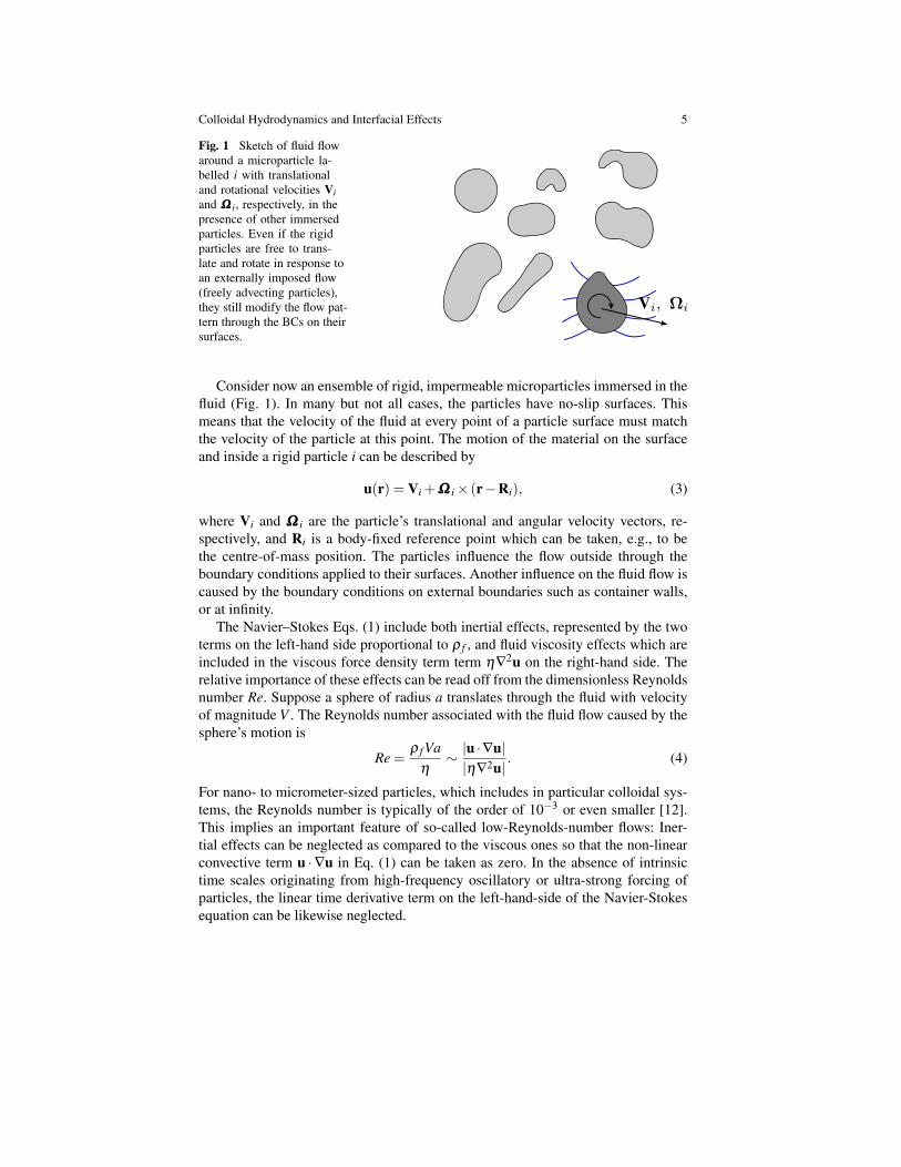
Fig. 1 Sketch of fluid flowaround a microparticle la-belled i with translationaland rotational velocities Viand ΩΩΩ i, respectively, in thepresence of other immersedparticles. Even if the rigidparticles are free to trans-late and rotate in response toan externally imposed flow(freely advecting particles),they still modify the flow pat-tern through the BCs on theirsurfaces.
Consider now an ensemble of rigid, impermeable microparticles immersed in thefluid (Fig. 1). In many but not all cases, the particles have no-slip surfaces. Thismeans that the velocity of the fluid at every point of a particle surface must matchthe velocity of the particle at this point. The motion of the material on the surfaceand inside a rigid particle i can be described by
u(r) = Vi +ΩΩΩ i× (r−Ri), (3)
where Vi and ΩΩΩ i are the particle’s translational and angular velocity vectors, re-spectively, and Ri is a body-fixed reference point which can be taken, e.g., to bethe centre-of-mass position. The particles influence the flow outside through theboundary conditions applied to their surfaces. Another influence on the fluid flow iscaused by the boundary conditions on external boundaries such as container walls,or at infinity.
The Navier–Stokes Eqs. (1) include both inertial effects, represented by the twoterms on the left-hand side proportional to ρ f , and fluid viscosity effects which areincluded in the viscous force density term term η∇2u on the right-hand side. Therelative importance of these effects can be read off from the dimensionless Reynoldsnumber Re. Suppose a sphere of radius a translates through the fluid with velocityof magnitude V . The Reynolds number associated with the fluid flow caused by thesphere’s motion is
Re =ρ fVa
η∼ |u ·∇u||η∇2u|
. (4)
For nano- to micrometer-sized particles, which includes in particular colloidal sys-tems, the Reynolds number is typically of the order of 10−3 or even smaller [12].This implies an important feature of so-called low-Reynolds-number flows: Iner-tial effects can be neglected as compared to the viscous ones so that the non-linearconvective term u ·∇u in Eq. (1) can be taken as zero. In the absence of intrinsictime scales originating from high-frequency oscillatory or ultra-strong forcing ofparticles, the linear time derivative term on the left-hand-side of the Navier-Stokesequation can be likewise neglected.
6 Maciej Lisicki and Gerhard Nagele
The description of microparticle-induced hydrodynamics in a Newtonian fluidreduces then to the Stokes equations,
−∇p(r)+η∇2u(r)+ f(r) = 0, (5)
∇ ·u(r) = 0, (6)
also referred to as creeping flow equations. These equations have no explicit timedependence and are linear in the velocity and pressure fields.
Eq. (5) expresses the balance, at any instant of time and for every fluid element,of pressure gradient, viscous and external force densities. In the absence of externalforce density, the instantaneous values of velocity and pressure, and consequentlythe fluid stress field, depend solely on the momentary configuration and shape ofparticles and system boundaries, and on the surface boundary conditions taken at theparticle surfaces and system boundaries. There is thus no dependence on the earlierflow history. Note that motion under Stokes flow conditions can be unsteady, withthe velocities of particles and surrounding fluid changing as a function of time. Animportant example illustrating this fact is the settling of a spherical particle towardsa stationary wall in its vicinity. This settling is discussed in Subsec. 4.7 in relationto the effect of lubrication. At any instant, however, the net force and torque on eachparticle and each fluid element are zero, with accordingly instantaneous linear force-velocity relations characteristic of non-inertial fluid and immersed microparticlesmotions. The flow and pressure fields pattern readjust quasi-instantaneously to themoving system boundaries and particle surfaces.
In consequence, the hydrodynamic drag force Fh and torque Th acting on a par-ticle due to its surface friction with the surrounding fluid are exactly balanced, ac-cording to
Fh +F = 0 ,Th +T = 0 , (7)
by a non-hydrodynamic ’external’ force F and torque T, respectively, caused by di-rect interactions with other particles and system boundaries, and by external forcefields. Only a force-free and torque-free particle will move quasi-inertia-free. Thereis an addition a so-called thermodynamic force contribution to F proportional to thesystem temperature T which accounts for the on average isotropic thermal bombard-ment of a microparticle by the surrounding fluid molecules. If viewed on the timeand length scales where creeping flow applies this bombardment leads to an erraticBrownian motion of the particles which persists even in the absence of additionalforce contributions to F.
The strength of the Brownian motion of a particle can be characterized by thediffusion time τD which is the time required by a particle to diffuse by Brownianmotion over a distance comparable to its size. For a spherical particle of radius a,this characteristic time is
τD =a2
D0 ∝ ηa3
T, (8)
Colloidal Hydrodynamics and Interfacial Effects 7
whereD0 =
kBTCηa
, (9)
is the single-sphere Stokes-Einstein translational diffusion coefficient. This coef-ficient decreases with increasing particle size and fluid viscosity, and it increaseswith increasing temperature T . The numerical coefficient C depends on the hydro-dynamic boundary condition for the flow at the sphere surface. According to [1]⟨
[R(t)−R(0)]2⟩= 6D0t , (10)
where D0 quantifies the magnitude of the mean-squared displacement, after the timespan t, of the position vector R of an isolated Brownian particle immersed in anunbounded fluid. The brackets denote here an average over an equilibrium ensembleof non-interacting Brownian particles.
The diffusion time grows strongly with increasing particle size. For water at roomtemperature as the suspending fluid, it increases from τD ∼ 5 ms for a = 0.1 µm toτD ∼ 0.3 h for a = 5 µm. Brownian motion is thus negligibly small for particles ofseveral micrometers in size or larger. These particles are therefore referred to as non-Brownian. A dispersion of non-Brownian particles requires external driving agentsto keep them in motion. This agent can be gravity, provided some of the particlesare lighter or heavier than the fluid, or an applied electric, magnetic or temperaturegradient field. Additionally, the particles are hydrodynamically moved by incidentflows created by moving system boundary parts (e.g., in cylindrical Couette cellflow) or applied pressure gradients (e.g., in pipe flow).
The distinguishing and to some extent surprising properties of fluid flows de-scribed by the Stokes equations, and of the associated microparticles motions, areand important theme of the present lecture notes, in addition to interfacial effectsrelated to the fluid dynamics. In our discussion we will make ample use of stream-lines pattern in order to visualize Stokes flow fields formed around particles in thebulk fluid and at interfaces. A streamline is tangential to the local velocity field atany fluid point, and for stationary flow it agrees with the pathway of a fluid element.For each streamline segment dr, we have thus
dr×u(r) = 0 . (11)
The three Cartesian components of this vectorial equation form a coupled set ofdifferential equations, for given u(r), from which the streamlines can be determined.
2.1.1 Hydrodynamic stresses
To every solution, u, p, of the Stokes equations, referred to as a Stokes flow so-lution, one can associate a fluid stress field described in terms of a stress tensor σσσ .This symmetric second-rank tensor consists of nine elements σi j with i, j ∈ 1,2,3which at a given fluid position r have values depending on the considered (rectan-
8 Maciej Lisicki and Gerhard Nagele
gular) coordinate system spanned by its three basis vectors e1,e2,e3. The stresstensor has the following physical meaning: Imagine a small planar surface elementdS in the fluid with unit normal vector n. The hydrodynamic drag force, dF, exertedby the fluid on this surface element, located on the side where n points to, is thengiven by dF = σσσ · ndS. The tensor (matrix) element σi j is therefore the hydrody-namic force component per unit area (referred to as stress) acting in the directionei on an areal element with normal vector equal to e j [17]. The stress field of anincompressible Newtonian fluid is given in terms of the flow fields u and p by
σσσ(r) =−p(r)I+ηE(r), (12)
where I is the unit tensor, and
E(r) = [∇u(r)]+ [∇u(r)]T (13)
is the symmetric fluid rate-of-strain tensor, with the superscript T denoting the trans-position operation.
While the polyadic tensor expression for σσσ(r) in Eqs. (12) and (13) applies toall coordinate systems, the explicit form of its elements depends on the selectedcoordinates [15]. In Cartesian coordinates where the orthonormal basis vectorse1,e2,e3 = ex,ey,ez are constant, the stress tensor elements are simply givenby
σi j =−pδi j +η
[∂ui
∂ r j+
∂u j
∂ ri
], (14)
where r1,r2,r3= x,y,z are the Cartesian components of the fluid element posi-tion vector r.
The hydrodynamic stress field depends on the properties of the fluid flow whichin turn is influenced by the characteristics of the particles and confining walls,namely their porosity and fluid permeability, and other non-hydrodynamic surfaceproperties such as surface charge density, van der Waals attraction etc. The knowl-edge of stresses in the fluid is of importance, since it allows for the calculation ofhydrodynamic drag forces and torques acting on bodies immersed in the fluid. It isalso of key importance for the calculation of rheological properties such as the ef-fective suspension viscosity of a fluid with immersed microparticles [21]. Once thehydrodynamic stresses are known, the hydrodynamic drag force and torque, Fh andTh, acting on a particle can be calculated as the sum (integral) of the local surfaceforce and torque contributions, respectively, according to
Fh =∫
SdSσσσ(r) ·n(r)
Th =∫
SdS (r−R)×σσσ(r) ·n(r) (15)
The surface S can be replaced by any fluid surface S∗ enclosing the consideredparticle without intersecting another one, provided there is no body force densityacting on the enclosed fluid part, since the hydrodynamic force and torque on a
Colloidal Hydrodynamics and Interfacial Effects 9
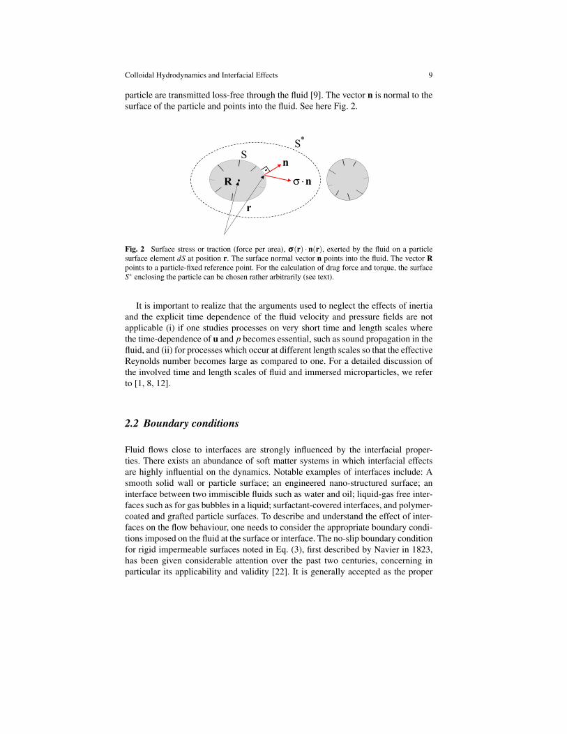
particle are transmitted loss-free through the fluid [9]. The vector n is normal to thesurface of the particle and points into the fluid. See here Fig. 2.
R
S S
*
n
r
σ ⋅n
Fig. 2 Surface stress or traction (force per area), σσσ(r) · n(r), exerted by the fluid on a particlesurface element dS at position r. The surface normal vector n points into the fluid. The vector Rpoints to a particle-fixed reference point. For the calculation of drag force and torque, the surfaceS∗ enclosing the particle can be chosen rather arbitrarily (see text).
It is important to realize that the arguments used to neglect the effects of inertiaand the explicit time dependence of the fluid velocity and pressure fields are notapplicable (i) if one studies processes on very short time and length scales wherethe time-dependence of u and p becomes essential, such as sound propagation in thefluid, and (ii) for processes which occur at different length scales so that the effectiveReynolds number becomes large as compared to one. For a detailed discussion ofthe involved time and length scales of fluid and immersed microparticles, we referto [1, 8, 12].
2.2 Boundary conditions
Fluid flows close to interfaces are strongly influenced by the interfacial proper-ties. There exists an abundance of soft matter systems in which interfacial effectsare highly influential on the dynamics. Notable examples of interfaces include: Asmooth solid wall or particle surface; an engineered nano-structured surface; aninterface between two immiscible fluids such as water and oil; liquid-gas free inter-faces such as for gas bubbles in a liquid; surfactant-covered interfaces, and polymer-coated and grafted particle surfaces. To describe and understand the effect of inter-faces on the flow behaviour, one needs to consider the appropriate boundary condi-tions imposed on the fluid at the surface or interface. The no-slip boundary conditionfor rigid impermeable surfaces noted in Eq. (3), first described by Navier in 1823,has been given considerable attention over the past two centuries, concerning inparticular its applicability and validity [22]. It is generally accepted as the proper
10 Maciej Lisicki and Gerhard Nagele
Effective (partial) slipLiquid interface
Fluid I
Fluid II
Perfect slip
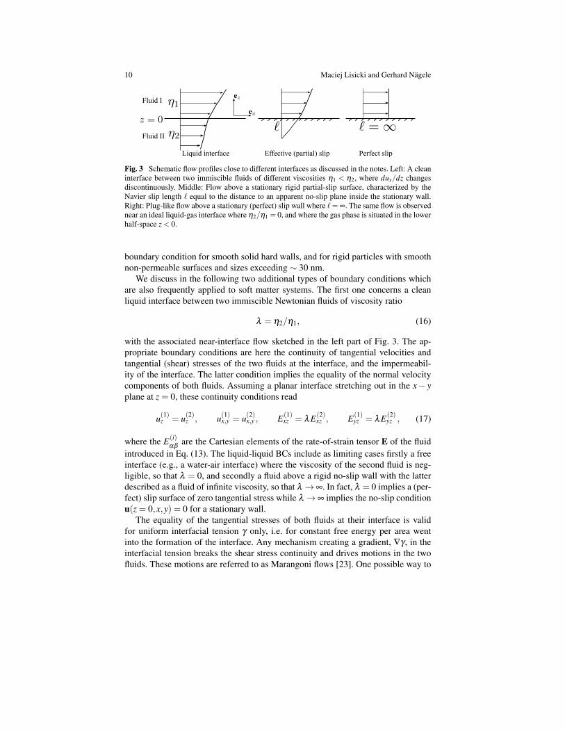
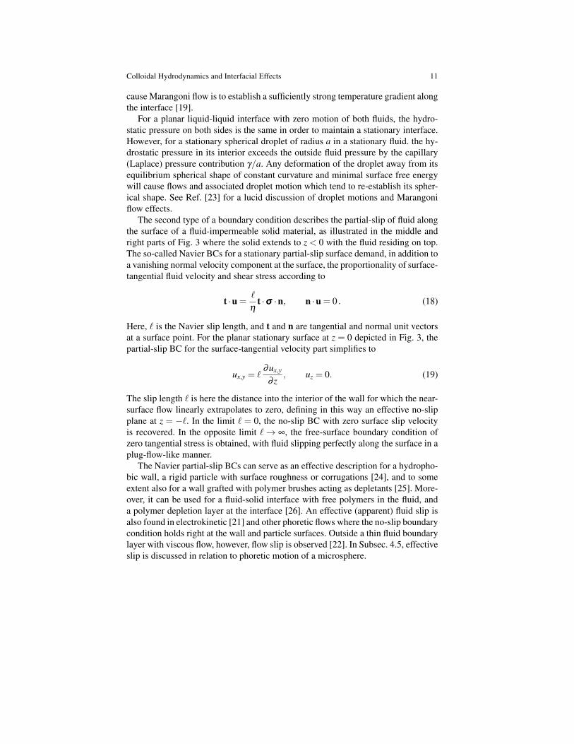
Fig. 3 Schematic flow profiles close to different interfaces as discussed in the notes. Left: A cleaninterface between two immiscible fluids of different viscosities η1 < η2, where dux/dz changesdiscontinuously. Middle: Flow above a stationary rigid partial-slip surface, characterized by theNavier slip length ` equal to the distance to an apparent no-slip plane inside the stationary wall.Right: Plug-like flow above a stationary (perfect) slip wall where `= ∞. The same flow is observednear an ideal liquid-gas interface where η2/η1 = 0, and where the gas phase is situated in the lowerhalf-space z < 0.
boundary condition for smooth solid hard walls, and for rigid particles with smoothnon-permeable surfaces and sizes exceeding ∼ 30 nm.
We discuss in the following two additional types of boundary conditions whichare also frequently applied to soft matter systems. The first one concerns a cleanliquid interface between two immiscible Newtonian fluids of viscosity ratio
λ = η2/η1, (16)
with the associated near-interface flow sketched in the left part of Fig. 3. The ap-propriate boundary conditions are here the continuity of tangential velocities andtangential (shear) stresses of the two fluids at the interface, and the impermeabil-ity of the interface. The latter condition implies the equality of the normal velocitycomponents of both fluids. Assuming a planar interface stretching out in the x− yplane at z = 0, these continuity conditions read
u(1)z = u(2)z , u(1)x,y = u(2)x,y , E(1)xz = λE(2)
xz , E(1)yz = λE(2)
yz , (17)
where the E(i)αβ
are the Cartesian elements of the rate-of-strain tensor E of the fluidintroduced in Eq. (13). The liquid-liquid BCs include as limiting cases firstly a freeinterface (e.g., a water-air interface) where the viscosity of the second fluid is neg-ligible, so that λ = 0, and secondly a fluid above a rigid no-slip wall with the latterdescribed as a fluid of infinite viscosity, so that λ →∞. In fact, λ = 0 implies a (per-fect) slip surface of zero tangential stress while λ →∞ implies the no-slip conditionu(z = 0,x,y) = 0 for a stationary wall.
The equality of the tangential stresses of both fluids at their interface is validfor uniform interfacial tension γ only, i.e. for constant free energy per area wentinto the formation of the interface. Any mechanism creating a gradient, ∇γ , in theinterfacial tension breaks the shear stress continuity and drives motions in the twofluids. These motions are referred to as Marangoni flows [23]. One possible way to
Colloidal Hydrodynamics and Interfacial Effects 11
cause Marangoni flow is to establish a sufficiently strong temperature gradient alongthe interface [19].
For a planar liquid-liquid interface with zero motion of both fluids, the hydro-static pressure on both sides is the same in order to maintain a stationary interface.However, for a stationary spherical droplet of radius a in a stationary fluid. the hy-drostatic pressure in its interior exceeds the outside fluid pressure by the capillary(Laplace) pressure contribution γ/a. Any deformation of the droplet away from itsequilibrium spherical shape of constant curvature and minimal surface free energywill cause flows and associated droplet motion which tend to re-establish its spher-ical shape. See Ref. [23] for a lucid discussion of droplet motions and Marangoniflow effects.
The second type of a boundary condition describes the partial-slip of fluid alongthe surface of a fluid-impermeable solid material, as illustrated in the middle andright parts of Fig. 3 where the solid extends to z < 0 with the fluid residing on top.The so-called Navier BCs for a stationary partial-slip surface demand, in addition toa vanishing normal velocity component at the surface, the proportionality of surface-tangential fluid velocity and shear stress according to
t ·u =`
ηt ·σσσ ·n, n ·u = 0 . (18)
Here, ` is the Navier slip length, and t and n are tangential and normal unit vectorsat a surface point. For the planar stationary surface at z = 0 depicted in Fig. 3, thepartial-slip BC for the surface-tangential velocity part simplifies to
ux,y = `∂ux,y
∂ z, uz = 0. (19)
The slip length ` is here the distance into the interior of the wall for which the near-surface flow linearly extrapolates to zero, defining in this way an effective no-slipplane at z = −`. In the limit ` = 0, the no-slip BC with zero surface slip velocityis recovered. In the opposite limit `→ ∞, the free-surface boundary condition ofzero tangential stress is obtained, with fluid slipping perfectly along the surface in aplug-flow-like manner.
The Navier partial-slip BCs can serve as an effective description for a hydropho-bic wall, a rigid particle with surface roughness or corrugations [24], and to someextent also for a wall grafted with polymer brushes acting as depletants [25]. More-over, it can be used for a fluid-solid interface with free polymers in the fluid, anda polymer depletion layer at the interface [26]. An effective (apparent) fluid slip isalso found in electrokinetic [21] and other phoretic flows where the no-slip boundarycondition holds right at the wall and particle surfaces. Outside a thin fluid boundarylayer with viscous flow, however, flow slip is observed [22]. In Subsec. 4.5, effectiveslip is discussed in relation to phoretic motion of a microsphere.
12 Maciej Lisicki and Gerhard Nagele
3 Generic features of Stokes flows
Creeping flows have interesting generic properties which appear counter-intuitivefrom the perspective of our macroscopic world experience where inertia and high-Reynolds-number effects prevail, with the flow governed by the non-linear Navier-Stokes equations. The three generic features of the Stokes equations are linearity,kinematic reversibility, and instantaneity. In this section, their implications for thecolloidal dynamics are described.
3.1 Linearity
The Stokes equations are linear in contrast to the underlying Navier-Stokes equa-tions. This means that the pressure, velocity and stress field are linearly related. Theconsequences of linearity are far-reaching. For instance, in a slow viscous channelflow, on doubling the applied pressure gradient a doubling of the flow rate is ob-tained. Moreover, a twofold increase in the rate of flow of viscous fluid through aporous medium will results in an unchanged pattern of streamlines of the flow, butwith the magnitude of the fluid elements velocities doubled. For a sphere settling ina viscous liquid, doubling the settling velocity gives rise to a correspondingly dou-bled hydrodynamic drag force. The fact that the hydrodynamic force on a particleand the associated velocity (increment) are linearly related is exploited further inSubsec. 4.1, where we discuss the hydrodynamic friction and mobility coefficientsin many-particle dispersions.
For linear evolution equations such as the Stokes equations, the superpositionprinciple is valid: If u1 and u2 are two velocity solutions of the Stokes equations,then
u = λ1u1 +λ2u2 (20)∇p = λ1∇p1 +λ2∇p2 (21)
are likewise solutions with coefficients λ1 and λ2. Here, ∇pi is the pressure gradientfield solution to the Stokes equations associated with ui. For a given flow problemboundary value problem, the unique velocity field u can be obtained from the lin-ear superposition of two (simpler) flows with unchanged geometry, provided thevelocity BCs of the two partial flows superimpose correspondingly, with the samecoefficients, to the BCs of the full flow solution.
The linearity of the Stokes flow solutions can lead to rather unexpected con-clusions; Consider a particle, moving through the fluid with the velocity V withCartesian components Vi, i = 1,2,3. The particle experiences then the drag force−F which we can decompose into forces acting along the axes of the coordinatesystem according to F = Fi. From linearity, we conclude that the force F1 actingon a particle moving with velocity (V1,0,0) must be of the form F1 = αV1, withα being a positive constant. Imagine now that the particle is a cube with its edges
Colloidal Hydrodynamics and Interfacial Effects 13
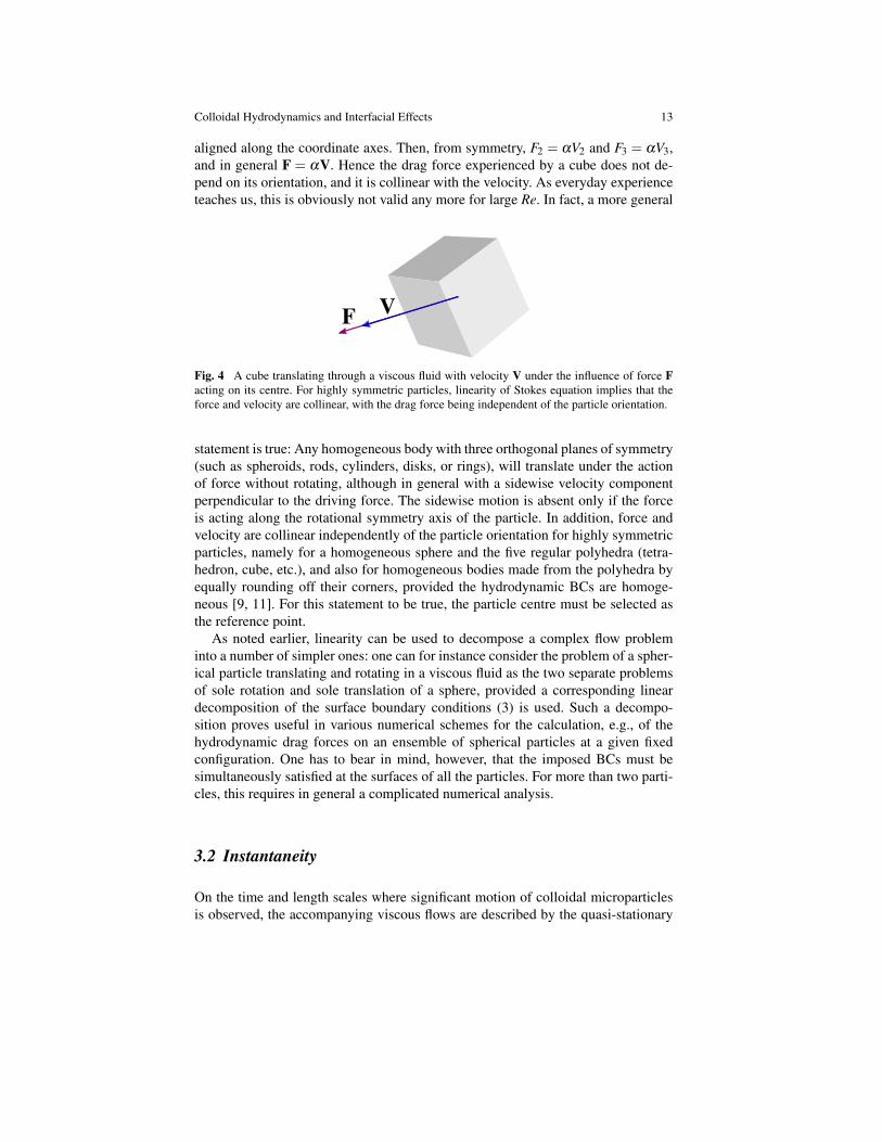
aligned along the coordinate axes. Then, from symmetry, F2 = αV2 and F3 = αV3,and in general F = αV. Hence the drag force experienced by a cube does not de-pend on its orientation, and it is collinear with the velocity. As everyday experienceteaches us, this is obviously not valid any more for large Re. In fact, a more general
Fig. 4 A cube translating through a viscous fluid with velocity V under the influence of force Facting on its centre. For highly symmetric particles, linearity of Stokes equation implies that theforce and velocity are collinear, with the drag force being independent of the particle orientation.
statement is true: Any homogeneous body with three orthogonal planes of symmetry(such as spheroids, rods, cylinders, disks, or rings), will translate under the actionof force without rotating, although in general with a sidewise velocity componentperpendicular to the driving force. The sidewise motion is absent only if the forceis acting along the rotational symmetry axis of the particle. In addition, force andvelocity are collinear independently of the particle orientation for highly symmetricparticles, namely for a homogeneous sphere and the five regular polyhedra (tetra-hedron, cube, etc.), and also for homogeneous bodies made from the polyhedra byequally rounding off their corners, provided the hydrodynamic BCs are homoge-neous [9, 11]. For this statement to be true, the particle centre must be selected asthe reference point.
As noted earlier, linearity can be used to decompose a complex flow probleminto a number of simpler ones: one can for instance consider the problem of a spher-ical particle translating and rotating in a viscous fluid as the two separate problemsof sole rotation and sole translation of a sphere, provided a corresponding lineardecomposition of the surface boundary conditions (3) is used. Such a decompo-sition proves useful in various numerical schemes for the calculation, e.g., of thehydrodynamic drag forces on an ensemble of spherical particles at a given fixedconfiguration. One has to bear in mind, however, that the imposed BCs must besimultaneously satisfied at the surfaces of all the particles. For more than two parti-cles, this requires in general a complicated numerical analysis.
3.2 Instantaneity
On the time and length scales where significant motion of colloidal microparticlesis observed, the accompanying viscous flows are described by the quasi-stationary
14 Maciej Lisicki and Gerhard Nagele
linear Stokes equations which have no explicit time dependence. As noted before,this means that the pressure and velocity fields adjust themselves instantaneously, onthe coarse-grained colloidal time and length scales, to changes in the driving forces.The flow disturbances propagate in the fluid with an (apparently) infinite speed. Aslight change in a particle’s position or velocity is instantaneously communicatedto the whole system. The fluid flow u, p at a given time is therefore fully de-termined by the instantaneous positions and velocities of the particle surfaces andwall boundaries, independently of how the momentary boundary values have beenreached (history independence). In particular, the instantaneous fluid flow patterndoes not depend on whether the boundary velocities will stay constant in the futureor change, such as in oscillatory motions.
This feature of Stokes flows appears counter-intuitive on the first sight. Yet, thereexist nice demonstrations highlighting its validity, provided the frequency of oscilla-tory boundary motions and the probed distances are not too large. Otherwise, hydro-dynamic retardation effects come into play reflecting the actually non-instantaneousspreading of flow perturbations by pressure (sound) waves, and by the diffusionalspreading of flow vorticity in the viscous fluid with an associated vorticity diffusioncoefficient, η/ρ f , equal to the kinematic viscosity [19, 27].
3.3 Kinematic reversibility
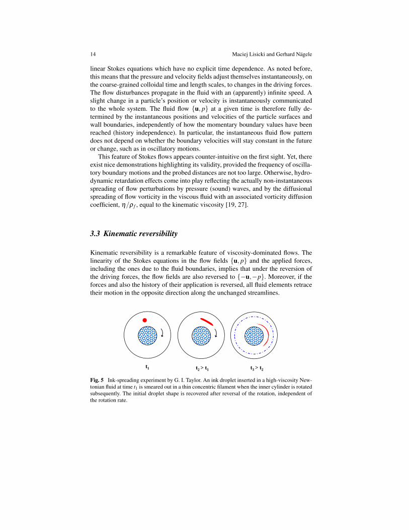
Kinematic reversibility is a remarkable feature of viscosity-dominated flows. Thelinearity of the Stokes equations in the flow fields u, p and the applied forces,including the ones due to the fluid boundaries, implies that under the reversion ofthe driving forces, the flow fields are also reversed to −u,−p. Moreover, if theforces and also the history of their application is reversed, all fluid elements retracetheir motion in the opposite direction along the unchanged streamlines.
t1 t2 > t1 t3 > t2
Fig. 5 Ink-spreading experiment by G. I. Taylor. An ink droplet inserted in a high-viscosity New-tonian fluid at time t1 is smeared out in a thin concentric filament when the inner cylinder is rotatedsubsequently. The initial droplet shape is recovered after reversal of the rotation, independent ofthe rotation rate.
Colloidal Hydrodynamics and Interfacial Effects 15
Kinematic reversibility was beautifully demonstrated in G. I. Taylor’s video [20]from 1966, where a drop of coloured ink is immersed in highly viscous glycerine, tomaintain low-Reynolds-number flow, filling the gap between two concentric cylin-ders (Couette cell geometry). See here Fig. 5. On rotating the inner cylinder, thedrop is smeared out along concentric streamlines into a thin filament. When the ro-tation is reversed subsequently by the same number of turns, the original dropletis reconstituted up to a small amount of blurring originating from the irreversibleresidual Brownian motion of the dye particles. The length of the filament dependson the number of turns only, independent of the rate at which the inner cylinder isrotated. This nicely illustrates the earlier discussed instantaneity of Stokes flows.
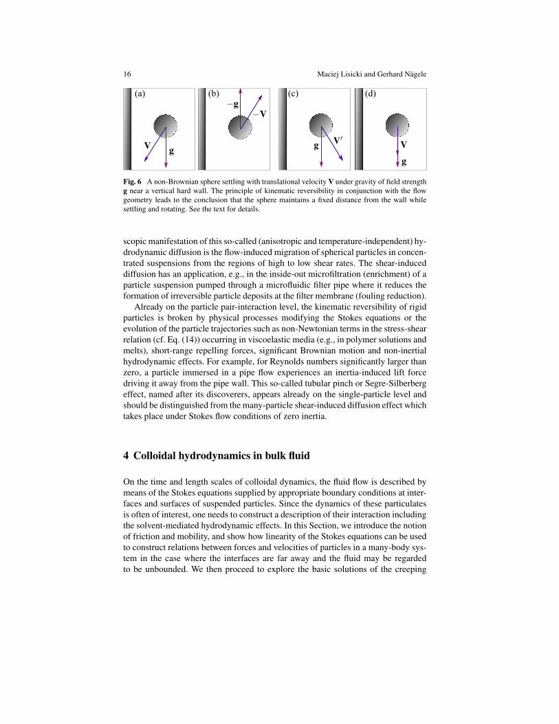
The kinematic reversibility in combination with specific symmetries puts generalconstraints on the motion of microparticle in a viscous fluid. A classical example isa spherical rigid microparticle settling under gravity near a stationary vertical hardwall (see Fig. 6). While the particle is rotating clockwise during settling, owing tothe larger wall-induced hydrodynamic friction on its semi-hemisphere facing thewall (see Subsec. 5.2 for details), a question arises whether it will approach the wallor recede from it. Given that gravity acts vertically downwards parallel to the wall,assume for the time being that the sphere approaches the wall while settling (see Fig.6(a)). Kinematic reversibility requires that once the direction of the motion-drivinggravitational force is reversed, the Stokes flow pattern remains unchanged except forthe directional reversal of the fluid elements motion, provided the translational andangular particle velocities are likewise reversed. According to Fig. 6(b), this impliesthat the sphere sediments upwards while receding from the wall. On rotating Fig.6(b) by 180 around the horizontal symmetry axis line going through the spherecentre, Fig. 6(c) is obtained in conflict with Fig. 6(a) wherein the sphere had beenassumed to approach the wall. A contradiction is avoided only if the sphere remainsat a constant distance from the wall while settling, as in Fig. 6(d). An analogousreasoning can be employed to show that in Poiseuille channel flow, a non-Brownianmicrosphere translates along the flow streamline, without any cross-flow velocitycomponent.
As discussed in Subsec. 5.3, a non-spherical rigid particle, such as a rod, canmove sidewise while settling and so approach the vertical wall. The wall-inducedrotation of the particle can lead to a subsequent motion away from the wall. A de-formable liquid droplet settling close to a vertical wall will deform into a shapewhich makes it glide away from the wall.
While non-spherical rigid particles and deformable particles can migrate acrossstreamlines under Stokes flow conditions, this is not the case for an isolated non-Brownian spherical particle. However, the non-linear hydrodynamic coupling of themotions of three or more nearby spheres in a driven system such as in the pipe flowof a suspension, can lead to irregularly looking trajectories which depend sensitivelyon the initial particle configuration. Any reversibility-breaking slight perturbationof the initial particle configuration caused, e.g., by direct particle interactions inthe form of surface roughness, flexibility or electric charge, or residual Brownianmotion and inertia effects, becomes exponentially amplified, giving rise to chaotictrajectories causing cross-stream migration and the mixing of the particles. A macro-
16 Maciej Lisicki and Gerhard Nagele
(a) (b) (c) (d)
Fig. 6 A non-Brownian sphere settling with translational velocity V under gravity of field strengthg near a vertical hard wall. The principle of kinematic reversibility in conjunction with the flowgeometry leads to the conclusion that the sphere maintains a fixed distance from the wall whilesettling and rotating. See the text for details.
scopic manifestation of this so-called (anisotropic and temperature-independent) hy-drodynamic diffusion is the flow-induced migration of spherical particles in concen-trated suspensions from the regions of high to low shear rates. The shear-induceddiffusion has an application, e.g., in the inside-out microfiltration (enrichment) of aparticle suspension pumped through a microfluidic filter pipe where it reduces theformation of irreversible particle deposits at the filter membrane (fouling reduction).
Already on the particle pair-interaction level, the kinematic reversibility of rigidparticles is broken by physical processes modifying the Stokes equations or theevolution of the particle trajectories such as non-Newtonian terms in the stress-shearrelation (cf. Eq. (14)) occurring in viscoelastic media (e.g., in polymer solutions andmelts), short-range repelling forces, significant Brownian motion and non-inertialhydrodynamic effects. For example, for Reynolds numbers significantly larger thanzero, a particle immersed in a pipe flow experiences an inertia-induced lift forcedriving it away from the pipe wall. This so-called tubular pinch or Segre-Silberbergeffect, named after its discoverers, appears already on the single-particle level andshould be distinguished from the many-particle shear-induced diffusion effect whichtakes place under Stokes flow conditions of zero inertia.
4 Colloidal hydrodynamics in bulk fluid
On the time and length scales of colloidal dynamics, the fluid flow is described bymeans of the Stokes equations supplied by appropriate boundary conditions at inter-faces and surfaces of suspended particles. Since the dynamics of these particulatesis often of interest, one needs to construct a description of their interaction includingthe solvent-mediated hydrodynamic effects. In this Section, we introduce the notionof friction and mobility, and show how linearity of the Stokes equations can be usedto construct relations between forces and velocities of particles in a many-body sys-tem in the case where the interfaces are far away and the fluid may be regardedto be unbounded. We then proceed to explore the basic solutions of the creeping
Colloidal Hydrodynamics and Interfacial Effects 17
flow equations for point forces which are the simplest approximation to the flowfield generated by the immersed particles. The set of solutions is then extended bymultipole expansion to include more subtle flow effects. We apply this formalism toinvestigate the motion of shape-anisotropic slender bodies, such as rod-like colloids,and later on construct a solution for a spherical particle moving through the fluid asa result of a force, or by a phoretic motion. We conclude this Section by a discussionof more advanced approaches to hydrodynamic interactions and of the lubricationeffects which are essential when the particles are very close together.
4.1 Friction and mobility of microparticles
We outline here the theoretical framework for the description of dynamics of a dis-persion consisting of N rigid microparticles of basically arbitrary shape evolvingunder Stokes flows conditions [14]. Consider the particles to be at the instantaneousconfiguration X = (R,ΘΘΘ) = (R1, . . . ,RN ,ΘΘΘ 1, . . . ,ΘΘΘ N), with body-fixed particle po-sition vectors Ri and orientations ΘΘΘ i. Here, ΘΘΘ i abbreviates the three Euler an-gles characterizing the orientation of the particle i.
Suppose now that the particles are subjected to external forces F = (F1, . . . ,FN)and torques T = (T1, . . . ,TN) where we have introduced 3N-dimensional super-vectors F and T for notational convenience. As a consequence of this forcing,motion of the particles and the fluid is induced, and the particles acquire quasi-instantaneously the translational velocities V = (V1, . . . ,VN) and the rotational ve-locities ΩΩΩ = (ΩΩΩ 1, . . . ,ΩΩΩ N). We have assumed a quiescent fluid for simplicity, mean-ing that the fluid would be at rest in the absence of particles. This implies, in par-ticular, that there is no ambient flow caused, e.g., by confining boundary parts inrelative motion. In the inertia-free Stokes flow system under consideration, each ex-ternal force and torque are balanced by hydrodynamic drag force and torque. Owingto the linearity of the Stokes equations and the hydrodynamic boundary conditions,the forces (torques) and translational (rotational) velocities are linearly related ac-cording to (
VΩΩΩ
)= µµµ(X) ·
(FT
), (22)
where the 6N×6N hydrodynamic mobility matrix µµµ has the four 3N×3N subma-trices
µµµ(X) =
(µµµ tt(X) µµµ tr(X)µµµrt(X) µµµrr(X)
). (23)
The superscripts tt and rr label the purely translational and rotational mobility ma-trix parts, respectively. The off-diagonal matrices with superscripts tr and rt de-scribe the hydrodynamic coupling between translational and rotational particle mo-tions. The tensor elements of these matrices have a straightforward physical mean-ing. To give an example, the tensor [µµµ tt(X)]i j relates the instant force F j on particlej with the translational velocity Vi of particle i, in a situation where particles differ-
18 Maciej Lisicki and Gerhard Nagele
ent from j are all force- and torque-free. The coupling tensor [µµµrt(X)]i j, on the otherhand, relates the force F j on particle j to the resulting angular velocity ΩΩΩ i of particlei. It is important to note here that the mobility matrix µµµ and its 4N2 mobility tensorelements depend on the configuration of the whole system, i.e. the instant positionsand orientations of all particles, as well as on the particle shapes and sizes, and thesurface boundary conditions. Finding the mobility tensor is therefore a very difficultproblem which for arbitrary particle shapes can be addressed only numerically for asmall number of particles.
It should be further noted that the form of the mobility matrix depends also on theselection of reference points R inside the particles. For these points, the so-calledcenter of mobility of each particle should be selected which in Stokes flow dynamicsplays a similar role as the center-of-mass position in Newtonian dynamics. For anaxisymmetric homogeneous rigid body, the center-of-mobility and the center-of-mass are both located on the symmetry axis but they coincide not necessarily. Theycoincide, however, for a homogeneous sphere. Different from the center-of-mass,the center-of-volume is depending on the shape of the particle surface only, foruniform surface BC, independent of the mass distribution inside the particle. For amore detailed discussion of this important issue, see [14, 28].
In the simplest case of hydrodynamically non-interacting spherical particles ofequal radius a, the tt and rr tensors reduce to the 3×3 unit matrices,
[µµµ tt(X)]i j = µt0δi j, [µµµrr(X)]i j = µ
r0δi j (24)
describing the free translation and rotation of isolated spheres. This limiting case isapproached for an ultra-dilute dispersion where the mean distance between two par-ticles is very large compared to their sizes. The single-particle mobility coefficientsof a no-slip sphere are explicitly (see Subsec. 5.2)
µt0 =
16πηa
, µr0 =
18πηa3 (25)
with Vi = µ t0Fi and ΩΩΩ i = µr
0 Ti. The tr and rt mobility tensors are here zero imply-ing that there is no coupling between the translational and rotational motion of theparticles.
Eq. (22) describes the so-called mobility problem where the forces and torquesacting on the particles are given, and the translational and rotational velocities aresearched for. The inverse problem where the velocities are given and the forces aresearched for, referred to as the friction problem, is straightforwardly formulated byintroducing the 6N×6N friction matrix
ζζζ = µµµ−1 . (26)
defined as the inverse of the mobility matrix. That this inverse exists is due to thefact that µµµ is symmetric and positive definite, for all physically allowed particle con-figurations. This follows from general principles of the Stokes flows, and it impliesphysically that the power supplied to the particles by external forces is completely
Colloidal Hydrodynamics and Interfacial Effects 19
and quasi-instantaneously dissipated by heating the fluid. We quantify this statementfor the motion of N torque-free microparticles in an infinite quiescent fluid wherethe rate of change of the particles kinetic energy, W (t), instantaneously dissipatedinto heat by friction is given by
0 <dW (t)
dt=
(FT
)·(
VΩΩΩ
)=
(FT
)·µµµ(X) ·
(FT
). (27)
Since the 6N-dimensional supervector with the particles forces and torques aselements is arbitrary, the second equality expresses the positive definiteness of the6N×6N symmetric mobility matrix µµµ tt . Any violation of the positive definiteness ofthis matrix would imply thus the violation of the second law of thermodynamics. Inspecializing Eq. (27) to torque-free and force-free particles, respectively, it followsreadily the positive definiteness likewise of the 3N×3N symmetric submatrices µµµ tt
and µµµrr for all physically allowed particle configurations X.The knowledge of the configuration-dependence of µµµ , or likewise that of ζζζ , al-
lows for exploration of the microparticles’ dynamics using numerical simulations,without having to address explicitly the accompanying fluid flow. For torque-freeparticles large enough for their Brownian motions to be negligible, the 3N coupledfirst-order equations of motion for the particles centre-of-mobility positions, in pres-ence of external and also non-hydrodynamic particle interaction forces all subsumedin F, are given by
dR(t)dt
= µµµtt (R(t)) ·F(t) . (28)
Integration of these evolution equations gives the positional trajectories of the parti-cles. This is referred to as Stokesian dynamics [29]. Due to the non-linearity of theStokesian dynamics evolution equations in Eq. (28), originating from the non-linearpositional dependence of the mobility matrix, the trajectories are highly sensitiveto the initial particle configuration: A slight change in the initial configuration canlead to large differences in the trajectorial evolution. Deterministic chaos in the tra-jectories of as little as three hydrodynamically interacting non-Brownian particlessettling under gravity has been observed first in the point-particle limit [30] and lateralso for extended spheres [31].
For smaller Brownian particles, on the other hand, the mobility matrix is neededas input not only for the generation of Stokesian particle displacements, but also forthe generation of additional stochastic displacements caused by the thermal fluc-tuations of the solvent. These displacements are the essential ingredients of theso-called Brownian dynamics numerical scheme for the generation of Brownianstochastic trajectories [32]. For a pedagogical introduction to Brownian dynamicssimulations, see [33]. From the generated trajectories, quantities such as the particlemean-squared displacement in Eq. (10) can be calculated, for the general case ofinteracting microparticles. The positive definiteness of the mobility matrix plays akey role for Brownian particles. It guarantees that a perturbed suspension evolvestowards thermodynamic equilibrium, in the absence of external forcing and ambientflow.
20 Maciej Lisicki and Gerhard Nagele
Complementary to the Stokesian dynamics and Brownian dynamics simulationschemes, the evolution of microparticle dispersions is studied theoretically also interms of the probability density distribution function P(X, t), where P(X, t)dX is theprobability of finding N particles at time t in a small 6N-dimensional neighbourhooddX of the configuration X. The evolution equations for P(X, t) for Brownian andnon-Brownian particles under Stokes-flow conditions are, respectively, the many-particle Smoluchowski diffusion equation and the Stokes-Liouville equation. Anintroductory discussion of these equations is given in Ref. [9].
4.2 Method of singularity flow solutions
Linearity of the Stokes equations allows for the representation of the fluid velocityand pressure in dispersions of microparticles in terms of a discrete or continuoussuperposition of elementary flow solutions. We discuss in the following a very usefulset of singularity incompressible flow solutions for an unbounded quiescent fluidwhich decay all to zero far away from a specified fluid point where they exhibit apole singularity [14, 34, 35]. For simple geometries, this set can be profitably usedto obtain, with little effort, exact Stokes flow solutions by linear superposition. Wewill exemplify this for the forced and phoretic motions of a microsphere, and forthe velocity field of a point force in front of a fluid-fluid interface (see Subsec. 5.1).To solve the latter problem, an image method is used similar to that in electrostatics[36]. For more complicated geometries such as for a complex-shaped particle, thesingularity method remains useful to gain information about the flow at far distancesfrom the particle, in the form of a multipolar series. We shall demonstrate this in ourdiscussion of the swimming trajectories of a self-propelling microswimmer near asurface.
The important observation is that for a given solution, u, p, of the homoge-neous Stokes equations, its derivatives are likewise flow solutions. We can thusconstruct a complete set of singularity solutions by taking derivatives of increas-ing order, of two fundamental flow solutions, namely those due to a point force anda point source.
We should add that for dispersions of spherical particles, specialized elementarysets of Stokes flow solutions can be constructed, which are different from the sin-gularity set discussed below, and which account for the high symmetry of spheres.These specific sets are used in numerically precise methods [37, 38] of calculatingthe many-sphere hydrodynamic mobility and friction coefficients required in Brow-nian and Stokesian dynamics simulations.
Point-force solution and Oseen tensor: The fundamental flow solutions, uSt, pSt,due to the body force density f(r) = δ (r− r0)F of a point force F = Fe, directedalong the unit vector e and acting on a quiescent, infinite fluid at a position r0, canbe obtained in several ways (see [39]). We only quote here the result
Colloidal Hydrodynamics and Interfacial Effects 21
uSt(r) = T(r− r0) ·F (29)
pSt(r) =1
4πUS(r− r0) ·F. (30)
The second-rank Oseen tensor, T(r), has the form
T(r) =1
8πη
1r(111+ rr) , (31)
where 111 is the unit tensor, r= rr, and rr is a dyadic tensor formed with the positionalunit vector r. In Cartesian coordinates, the Oseen tensor elements read
Ti j =1
8πη
(δi j
r+
rir j
r3
). (32)
The pressure field pSt(r) due to the point force at r0 is expressed here in terms ofthe elementary source vector field
US(r) =rr2 =−∇
1r. (33)
If multiplied by a constant c > 0 with the dimension of volume per time, c US(r)describes the radially directed outflow of fluid from the source point r0 = 0. Theflow rate through a surface S enclosing the source point is thus equal to
c∫
SdSUS ·n = 4πc . (34)
The elementary velocity field uSt(r) of a point-force is called a Stokeslet ofstrength F in the direction of e, and with the centre at r0 where it has a simple polesingularity. Note here that Ti j is the i-th component of the Stokeslet velocity fieldgenerated by a unit force acting in the j direction. The streamlines of the Stokesletare drawn as dashed lines in the left part of Fig. 9, together with those generatedby a spherical no-slip particle subjected to the same force. The hydrodynamics ofa translating sphere is discussed in detail further down. A significant difference be-tween the two streamlines pattern exterior to the impermeable sphere is visible onlynear its surface. The streamlines generated by the translating sphere are further outindistinguishable from those of the point-force Stokeslet.
The Stokeslet velocity field decays like 1/r at far distances from the point force.This slow decay can be ascribed to the conservation of momentum injected intothe fluid by the point force, which is spread out quasi-instantaneously. It createsmajor difficulties in dealing theoretically with the hydrodynamics of suspensions,since forced velocity disturbances influence even well-separated particles. An ad-ditional difficulty is that the hydrodynamic interactions between three and morenon-point-like particles is not pairwise additive, i.e. the hydrodynamic interactionsof two nearby particles is changed in a rather complicated way if a third one is intheir vicinity.
22 Maciej Lisicki and Gerhard Nagele
According to Eq. (33), the pressure field of a point force decays faster than thevelocity field by the factor of 1/r. Note that the pressure itself, and not just itsgradient, has been uniquely specified by demanding p→ 0 for r→ ∞. EmployingEq. (14), the stress on a fluid surface element at position r and normal n, due to apoint force at the coordinate system origin, is
σσσSt(r) ·n(r) =−3
4πF ·(
rrrr2
)·n =− 3
4π
(r ·F)(r ·n)r2 r . (35)
On integrating the stress over a surface enclosing the point force, the expected resultFh =−F is obtained.
That the pressure field decays by the factor 1/r faster than the associated velocityfield is a general rule. It follows from the homogeneous Stokes equation written inthe form ∇p = η∇2u, where the first-order derivatives of p are expressed by thesecond-order derivatives of u. It can be also noticed here that the pressure in Stokesflows is a subsidiary quantity, fully determined by the velocity field for BCs invokingvelocities only. The velocity field can be calculated without reference to the pressureas a solution of the bi-harmonic differential equation
∇2∇
2u(r) = 0 , (36)
which readily follows from the application of the divergence operation to the homo-geneous Stokes equation, using in addition the flow incompressibility constraint.
For completeness, consider also the vorticity field, ∇× u(r), associated with avelocity field u(r). The vorticity is twice the angular velocity of a fluid element atr. The vorticity due to a point force at position r0 is
∇×uSt(r) =−1
4πηUS(r− r0)×F , (37)
identifying the Stokeslet as an incompressible rotational flow solution.The Oseen tensor for an unbounded infinite fluid is of key importance not only in
generating higher-order elemental force singularity solutions (see below), but alsofor the so-called boundary integral method of calculating the flow around complex-shaped bodies. The disturbance flow, i.e. the flow taken relative to a given ambientflow field uamb(r), observed in the exterior of a rigid no-slip particle in infinite fluidis given by the integral
u(r)−uamb(r) =∫
Sp
dS′T(r− r′) ·σσσ(r′) ·n(r′) , (38)
over the particle surface Sp, i.e. by a continuous superposition of surface-locatedStokeslets of vectorial strength σσσ · n. We emphasize here that if the fluid at Sp istangentially mobile such as for a rigid particle with Navier partial-slip BC, and aliquid droplet or gas bubble, there is an additional surface integral contribution tothe exterior flow. The form of this additional contribution is discussed in detail intextbooks on low-Reynolds-number fluid dynamics [14, 35, 40].
Colloidal Hydrodynamics and Interfacial Effects 23
The ambient velocity field uamb(r) is a Stokes flow caused by sources exterior tothe considered particle. In a non-quiescent situation it can be, e.g., a linear shear orquadratic Poiseuille flow. The ambient flow can be also the flow due to the motionof other rigid or non-rigid particles. If the considered particle was not present, theambient flow would be measured in the system.
Integrating Eq. (38) with respect to r over the particle surface, and using the no-slip BC in Eq. (3) for its left-hand side, results in a linear surface integral equationfor the surface stress field σσσ · n in terms of the given translational and rotationalparticle velocities V and ΩΩΩ , and the ambient flow field (friction problem). The in-tegral equation can be solved numerically by an appropriate surface discretization(triangulation). For given particle force and torque (mobility problem), and givenambient flow, the velocities are determined from substituting the calculated stressfield into the likewise discretized Eq. (15) for Fh and Th. See here [8, 9, 35] fordetails on the boundary integral method which has the main advantage of requiringonly a two-dimensional surface mesh for a three-dimensional flow calculation.
Force multipoles solutions: Singularity solutions of increasing multipolar orderare obtained from derivatives of the fundamental flow solution uSt(r). They alsoshow up in the expansion of uSt in a Taylor series about the force placement (sin-gularity) point r0. Recall now that point force F = Fe oriented along the direction egenerates the velocity field
uSt(r− r0) =F
8πηG(r− r0;e) , (39)
withG(r;e) = 8πηT(r) · e = e
r+
e · rr3 r . (40)
We select G(r;e) as the starting element of the singularity set, quoting it as thefundamental e-directed Stokeslet. It is actually equal to a Stokeslet of unit force inthe direction e, made non-dimensional by multiplication with 8πη and division bythe force unit. The first two singularity solutions obtained from directional deriva-tives of the fundamental Stokeslet are the Stokeslet doublet GD, and the Stokesletquadrupole GQ [26, 41]
GD(r− r0;d,e) = (d ·∇0)G(r− r0;e)∼O(r−2) , (41)
GQ(r− r0;c,d,e) = (c ·∇0)GD(r− r0;d,e)∼ O(r−3) , (42)
where the gradient operator ∇0 acts on the singularity placement r0, and d and care arbitrary vectors. We have indicated here the decay of these velocity fields fardistant from the singularity point. Higher-order singularity flow solutions with anO(r−4) asymptotic decay are obtained accordingly by repeated differentiation. Forlater use, we explicitly quote the Stokeslet doublet,
24 Maciej Lisicki and Gerhard Nagele
GD(r;d,e) = d · 1r2
[r1−1r− T(r1)+3 rrr
]· e (43)
=1r2
[e(r ·d)−d(r · e)− (d · e)r+3(r · e)(r ·d)r
]. (44)
where the pre-transposition symbol implies the interchange of the first two Carte-sian indices. The Stokes doublet GD(r; d,e), with d denoting a unit vector, has thefollowing physical interpretation: It is the velocity field times 8πη , of two opposingStokelets of vector strengths ±Fe and singularity locations at r0±d (with d = dd),in the limits d→ 0 and F→∞ with the force dipole moment p = 2Fd kept constantequal to one. The unit vector d points from the Stokeslet of strength −Fe to the oneof strength Fe. This interpretation is obviated from the explicit calculation of theflow field,
uD(r) =[T(r− r0−d)−T(r− r0 +d)
]· eF = 2dF
(d ·∇0
)T(r− r0) · e+O(d2)
=p
8πηGD(r− r0; d,e)+O(d2) . (45)
The force doublet provides the far-field behaviour of flows caused by force-freemicroparticles. It is named asymmetric when d is not collinear with the force di-rection ±e, and referred to as symmetric otherwise. The symmetric force doubletGD(r− r0;e,e) is also called a linear force dipole. It plays a major role in the dis-cussion of the flow created by many autonomous microswimmers, including vari-ous types of prokaryotic bacteria and eukaryotic unicellular microorganisms. Mi-croswimmers in the bulk fluid and near interfaces are discussed in Sec. 6.
The force doublet can be split into an anti-symmetric part, named Rotlet R, and asymmetric part named Stresslet S, each of which has a direct physical meaning. Weexemplify this for the Rotlet and in the special situation where the force strengths ofthe two opposing Stokeslets are orthogonally displaced, and aligned with the z-axisand x-axis, respectively. Then, F ·d = 0 and the dipole moment T = 2dF has themeaning of an applied torque. The Rotlet at the singularity point r0 = 0 is in thiscase
R(r;−ey) =12[GD(r;ex,ez)−GD(r;ez,ex)] =−ey×
rr2 , (46)
and after division by the factor 8πη it describes the rotational flow field due to aunit point torque aligned with the negative y-axis.
The symmetric Stresslet part reads
S(r;e±) =12[GD(r;ex,ez)+GD(r;ez,ex)] =
3 rr2 (r · ex)(r · eZ)
= GD(r;e+,e+)−GD(r;e−,e−) . (47)
It describes a straining fluid motion [14] originating from the superposition two lin-ear force dipoles oriented along the diagonal stretching axis e+ and the anti-diagonalcompression axis e−, respectively, where e± = (ex± ez)/
√2. The streamlines of a
linear force dipole are discussed in Sec. 6, and are drawn in Fig. 27.
Colloidal Hydrodynamics and Interfacial Effects 25
- - -
-
-
-
(a) Stokeslet G(ez)∼O(r−1)
+
- - -
-
-
-
(b) Source US(r)∼ O(r−2)
- - -
-
-
-
(c) Stokeslet doublet GD(r;ex,ez)∼O(r−2)
- - -
-
-
-
(d) Stresslet S(r;e±)∼ O(r−2)
- - -
-
-
-
(e) Rotlet R(r;−ey)∼ O(r−2)
+-
- - -
-
-
-
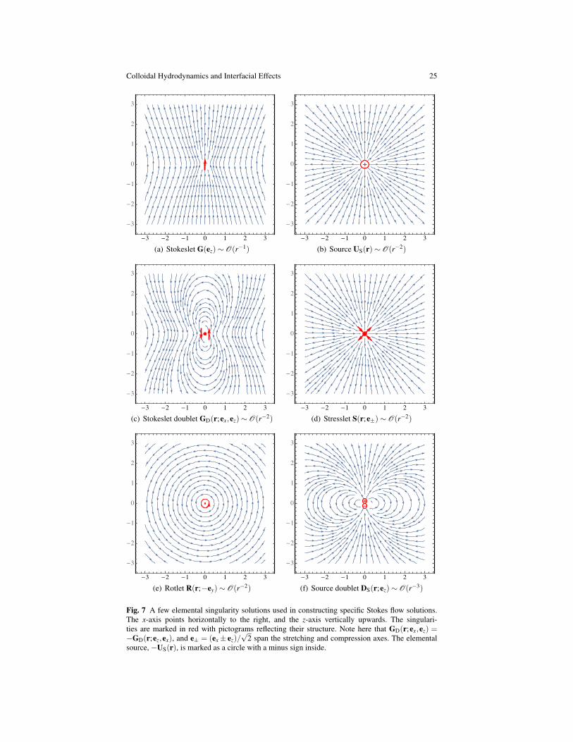
(f) Source doublet DS(r;ez)∼ O(r−3)
Fig. 7 A few elemental singularity solutions used in constructing specific Stokes flow solutions.The x-axis points horizontally to the right, and the z-axis vertically upwards. The singulari-ties are marked in red with pictograms reflecting their structure. Note here that GD(r;ex,ez) =−GD(r;ez,ex), and e± = (ex± ez)/
√2 span the stretching and compression axes. The elemental
source, −US(r), is marked as a circle with a minus sign inside.
26 Maciej Lisicki and Gerhard Nagele
The key point to notice here is that the stresses σσσS ·n and σσσR ·n, associated withthe Stresslet and Rotlet force doublet parts, respectively, are decaying as O(1/r3).When these stresses are integrated over a surface enclosing the singularity point,according to Eq. (15) they do not contribute a hydrodynamic drag force. Differ-ently from the Stresslet which is torque-free, the Rotlet contributes a hydrodynamictorque of magnitude equal to 8πη times the torque unit. The stress fields of all thehigher-order force singularity solutions including the one by the force quadrupoleGQ are all of O(1/r4), so that they contribute neither a drag force nor a torque [8, 9].
Source multipoles solutions: Elementary singularity solutions in addition to theforce singularities are obtained from derivatives of the source vector field US(r−r0)in Eq. (33) with respect to the singularity (source) point r0. The two leading-orderflows obtained in this way are the source doublet (dipole) and quadrupole,
DS(r− r0;e) = (e ·∇0)US(r− r0)∼O(r−3) (48)QS(r− r0;d,e) = (d ·∇0)DS(r− r0;e)∼ O(r−4) . (49)
The source doublet multiplied by a constant c of dimension volume per time de-scribes the flow due to a source flow with outflow rate 4πc, and a sink flow of thesame inflow rate. The source at r0 + de and the sink of the doublet at r0− de arean infinitesimal vector distance 2de separated from each other and have the moment2dc equal to one. Explicitly,
DS(r;e) =1r3
[3 rr−1
]· e = 1
r3
[3(r · e) r− e
]. (50)
The source singularity solutions are related to the force singularity solutions by
DS(r− r0) =−12
∇20G(r− r0) , (51)
and its derivatives. Eq. (51) identifies the source doublet as a degenerate forcequadrupole, which explains its faster decay than that of the force doublet. The stressfields of the source multipoles decay as O(1/r4) or faster, except for the source flowUS itself, implying that they make no force and torque contributions. As the deriva-tives of the Coulomb-type potential 1/r (see Eq. (33)), the source multipoles belongto the class of irrotational potential flows (where ∇×u = 0) with associated con-stant pressure fields. To understand the pressure constancy, note with u = ∇ψ forsome scalar (potential) function that incompressibility implies ∆ψ = 0. It followswith the Stokes equation that ∇p = η∆ (∇ψ) = η∇(∆ψ) = 0.
Superposition of singularity solutions: Linear superposition of fundamental sin-gularity solutions, appropriately selected and positioned to conform with the systemsymmetry and BCs under consideration, can be profitably used to construct (approx-imate) flow solutions. The coefficients in the superposition series can be determinedfrom the prescribed BCs.
Colloidal Hydrodynamics and Interfacial Effects 27
As an example of such a superposition, in Subsec. 4.3 we discuss the gravitationalsettling of a slender body whose flow field can be described in decent approximationby a continuous distribution of Stokeslets placed along the body’s center line.
For a particle axisymmetric along the direction e, and in a flow situation shar-ing this axial symmetry, the appropriate superposition describing the far-distancevelocity field is
u(r) = c1 (aG(r;e))+ c2(a2 GD(r;e;e)
)+ c3
(a3 SD(r;e)
)+O(r−4) , (52)
with scalar coefficients ci having the physical dimension of a velocity. The cen-troid r0 of the particle placed is placed here in the origin, and a can be taken as thelateral length of the particle. The Rotlet part of the symmetric force doublet GD iszero here, since a torque-free, non-rotating particle is required by the symmetry ofthe flow problem. If the particle moves force-free along its axial direction, as it is thecase for a self-propelling microswimmer, there is no Stokeslet contribution so thatc1 = 0. On the other hand, if the particle is sedimenting along its axis, the co-lineardriving force is given by
F = c1 (8πηa)e , (53)
with the coefficient c1 determining the strength of the Stokeslet depending on theparticle BCs. In Subsec. 4.4, we show that the flow created by a sphere translatingthrough a quiescent fluid, is exactly represented by the superposition of a Stokesletand a source dipole, owing to the high symmetry of this flow problem. If the sphereis placed in an ambient linear shear flow where the stress distribution on its surfacebecomes non-uniform, then a more general superposition of singularity solutionsmust be used including a source quadrupole, which in addition accounts for all rele-vant Cartesian directions, to obtain the exact flow solution [42]. Note also that for atranslating spheroid, a line distribution of Stokeslets and source doublets extendingbetween the focal points must be used [34]. As it is explained in Sec. 5.1, an appro-priate placement of elemental singularity solutions at a reflection point provides ananalytic solution for the velocity field of a point force in the presence of a fluid-fluidinterface.
4.3 Slender body motion
As a first application, we use the force singularity method to determine the hydrody-namic friction experienced by a settling rigid slender body, that is a particle withoutsharp corners whose contour length, L, is large compared to its thickness d. Exam-ples of such bodies include rod-like particles, and elongated or prolate spheroids.Owing to the shape anisotropy, the friction force depends on the orientation of thebody relative to the direction of motion. The slenderness of the body renders it pos-sible, in place of having to solve a complicated boundary integral problem for a no-slip particle on the basis of Eq. (38), to describe approximately the disturbance flow
28 Maciej Lisicki and Gerhard Nagele
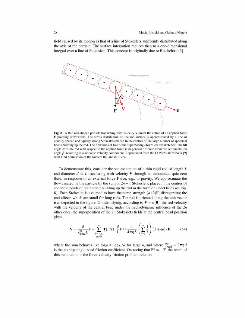
field caused by its motion as that of a line of Stokeslets, uniformly distributed alongthe axis of the particle. The surface integration reduces then to a one-dimensionalintegral over a line of Stokeslets. This concept is originally due to Batchelor [43].
1"
VF e
βα
Fig. 8 A thin rod-shaped particle translating with velocity V under the action of an applied forceF pointing downwards. The stress distribution on the rod surface is approximated by a line ofequally-spaced and equally strong Stokeslets placed in the centres of the large number of sphericalbeads building up the rod. The flow lines of two of the superposing Stokeslets are sketched. The tiltangle α of the rod with respect to the applied force is in general different from the sedimentationangle β , resulting in a sidewise velocity component. Reproduced from the COMPLOIDS book [9]with kind permission of the Societa Italiana di Fisica.
To demonstrate this, consider the sedimentation of a thin rigid rod of length Land diameter d L translating with velocity V through an unbounded quiescentfluid, in response to an external force F due, e.g., to gravity. We approximate theflow created by the particle by the sum of 2n+1 Stokeslets, placed in the centres ofspherical beads of diameter d building up the rod in the form of a necklace (see Fig.8). Each Stokeslet is assumed to have the same strength (d/L)F, disregarding theend effects which are small for long rods. The rod is oriented along the unit vectore as depicted in the figure. On identifying, according to V = u(0), the rod velocitywith the velocity of the central bead under the hydrodynamic influence of the 2nother ones, the superposition of the 2n Stokeslets fields at the central bead positiongives
V =d
ζ 0beadL
F+n
∑i=−n,n6=0
T(ide) · dL
F≈ 14πηL
(n
∑i=1
1i
)(111+ ee) ·F, (54)
where the sum behaves like logn ≈ logL/d for large n, and where ζ 0bead = 3πηd
is the no-slip single-bead friction coefficient. On noting that Fh =−F, the result ofthis summation is the force-velocity friction problem relation
Colloidal Hydrodynamics and Interfacial Effects 29
Fh =−[ζ
tt‖ ee+ζ
tt⊥(111− ee)
]·V, (55)
and likewise the inverse relation,
V =−[µ
tt‖ ee+µ
tt⊥(111− ee)
]·Fh , (56)
for the mobility problem of given force. The friction and mobility coefficients for thetranslation of a thin rod parallel and perpendicular to its axis e have been obtainedhere as
ζtt‖ =
1µ tt‖=
2πηLlog(L/d)
, ζtt⊥ =
1µ tt⊥= 2ζ
tt‖ . (57)
Corrections to this asymptotic result from a refined hydrodynamic calculation for acylinder with end effects included are provided in [44]. Note that the application,i.e. dot-multiplication, of the dyadic (111−ee) to a vector gives the component of thisvector perpendicular to e.
Remarkably, the friction coefficient for the broadside motion of a thin rod is onlytwice as large as that for the axial motion. Both coefficients scale essentially withthe length L of the rod, so that the drag force acting on a thin rod is not far less thanthat experienced by a sphere of diameter L enclosing it. It should be noted here thatfrom general properties of Stokes flows it follows that the magnitude of the dragforce on an arbitrarily-shaped body is always in between those for the inscribingand enclosing spheres [8, 14].
It is interesting to analyse the effect of the friction anisotropy on the directionof sedimentation. Denoting as α the angle between the rod axis e and the appliedforce F, and as β the angle between rod velocity and applied force, we can relatethe two angles by decomposing the external force into its components along andperpendicular to the rod axis, with the accompanying components of V determinedby the mobility coefficients. In this way, one obtains
β = α− arctan( 1
2 tanα). (58)
For a vertically or horizontally oriented rod and the applied force pointing down-wards (see again Fig. 8), there will be no sidewise rod motion due to symmetry.Except for these special configurations, however, the tilt angle α of the rod is differ-ent from its sedimentation angle β , although both will remain constant during themotion. The maximum settling angle βmax = arctan(
√2/4)≈ 19.5 corresponds to
α ≈ 54.7.Kinematic reversibility in conjunction with the system symmetry (no nearby
walls are present here) commands that the rod is settling without rotation. The fric-tion asymmetry of rod-shaped particles discussed here is a key ingredient in theswimming strategy of microswimmers with helical flagellar propulsion.
An elementary introduction to the concept of slender body motion is containedin the works [11, 14]. For a general discussion of slender bodies, which may also becurved, see [45, 46].
30 Maciej Lisicki and Gerhard Nagele
4.4 Forced translation of a microsphere
We consider here a microsphere of radius a with Navier partial slip BCs, whichtranslates with constant velocity V0 = V0e and without rotation through an un-bounded quiescent fluid. The origin of the coordinate system is placed at the mo-mentary sphere center. We attempt to describe the exterior fluid velocity (r ≥ a) bythe linear superposition of a Stokeslet and source doublet in accord with Eq. (52),and with the coefficients c1 and c3 determined by the BCs. It is convenient to expressu = ur r+uθ eθ and V0 =V0,r r+V0,θ eθ in polar coordinates with components
ur(r,θ) = 2cosθ
[c1
(ar
)+ c3
(ar
)3], V0,r =V0 cosθ
uθ (r,θ) =−sinθ
[c1
(ar
)− c3
(ar
)3], V0,θ =−V0 sinθ (59)
where e · r = cosθ and e · eθ = −sinθ have been used, with θ denoting the anglebetween polar axis e and fluid position vector r. The two coefficients can be deter-mined from enforcing the BC of zero normal velocity difference between the sphereand the fluid at the surface, ur(a,θ) = V0,r, in conjunction with the Navier partialslip condition in Eq. (18) for the tangential velocity part. The latter is formulated interms of the fluid velocity in the particle rest frame,
u′(r) = u(r)−V0 , (60)
labelled by the prime, where the fluid far away from the stationary sphere is movingwith uniform velocity −V0. The Navier BC reads
u′θ (r,θ) =`
η
(∂u′
θ
∂ r−
u′θ(r,θ)a
), (r = a) (61)
The two coefficients are determined from the BCs as
c1 =3V0
4
(1+2`∗
1+3`∗
), c3 =−
V0
4
(1
1+3`∗
), (62)
where `∗ = `/a.Using Eq. (53), the hydrodynamic drag force opposing the motion of the sphere
follows from the Stokeslet contribution as
Fh =−(8πηac1)e =−6πηa(
1+2`∗
1+3`∗
)V0 . (63)
Note that the single-sphere friction coefficient, ζ t0 = 1/µ t
0, relating the velocity ofan isolated sphere to its drag force according to
Fh =−ζt0 V0 , (64)
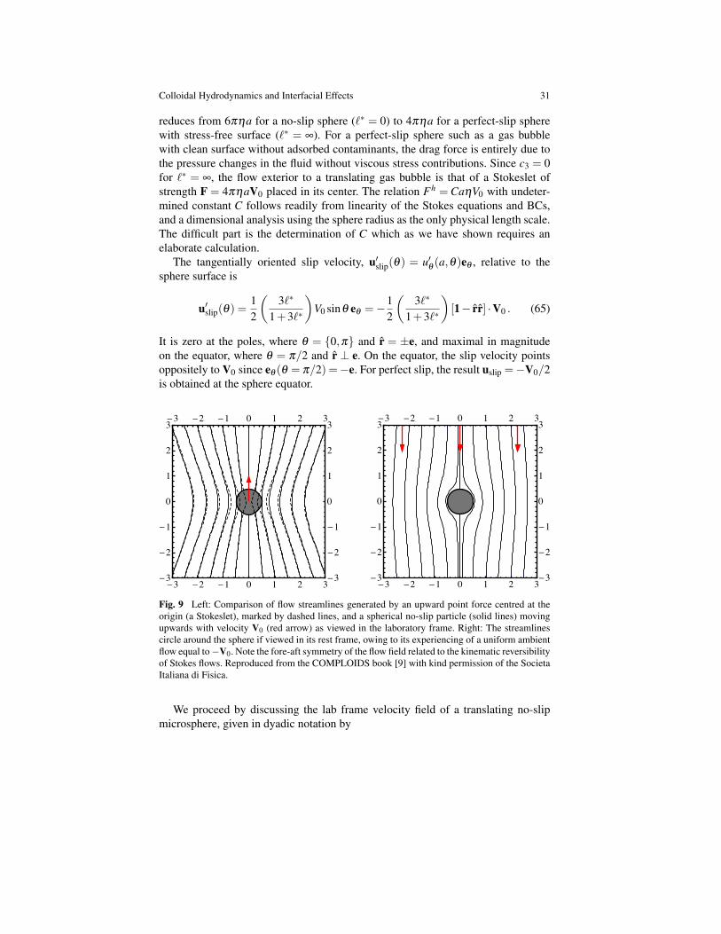
Colloidal Hydrodynamics and Interfacial Effects 31
reduces from 6πηa for a no-slip sphere (`∗ = 0) to 4πηa for a perfect-slip spherewith stress-free surface (`∗ = ∞). For a perfect-slip sphere such as a gas bubblewith clean surface without adsorbed contaminants, the drag force is entirely due tothe pressure changes in the fluid without viscous stress contributions. Since c3 = 0for `∗ = ∞, the flow exterior to a translating gas bubble is that of a Stokeslet ofstrength F = 4πηaV0 placed in its center. The relation Fh = CaηV0 with undeter-mined constant C follows readily from linearity of the Stokes equations and BCs,and a dimensional analysis using the sphere radius as the only physical length scale.The difficult part is the determination of C which as we have shown requires anelaborate calculation.
The tangentially oriented slip velocity, u′slip(θ) = u′θ(a,θ)eθ , relative to the
sphere surface is
u′slip(θ) =12
(3`∗
1+3`∗
)V0 sinθ eθ =−1
2
(3`∗
1+3`∗
)[1− rr] ·V0 . (65)
It is zero at the poles, where θ = 0,π and r = ±e, and maximal in magnitudeon the equator, where θ = π/2 and r ⊥ e. On the equator, the slip velocity pointsoppositely to V0 since eθ (θ = π/2) =−e. For perfect slip, the result uslip =−V0/2is obtained at the sphere equator.
-3 -2 -1 0 1 2 3-3
-2
-1
0
1
2
3-3 -2 -1 0 1 2 3
-3
-2
-1
0
1
2
3
-3 -2 -1 0 1 2 3-3
-2
-1
0
1
2
3-3 -2 -1 0 1 2 3
-3
-2
-1
0
1
2
3
Fig. 9 Left: Comparison of flow streamlines generated by an upward point force centred at theorigin (a Stokeslet), marked by dashed lines, and a spherical no-slip particle (solid lines) movingupwards with velocity V0 (red arrow) as viewed in the laboratory frame. Right: The streamlinescircle around the sphere if viewed in its rest frame, owing to its experiencing of a uniform ambientflow equal to−V0. Note the fore-aft symmetry of the flow field related to the kinematic reversibilityof Stokes flows. Reproduced from the COMPLOIDS book [9] with kind permission of the SocietaItaliana di Fisica.
We proceed by discussing the lab frame velocity field of a translating no-slipmicrosphere, given in dyadic notation by
32 Maciej Lisicki and Gerhard Nagele
u(r) =[(a
r
)(111+ rr)− 1
3
(ar
)3(3rr−111)
]· F
8πηa, (66)
with F = 6πηaV0, and with r measuring the distance from the center of the sphere.This result has been first calculated by Stokes more than 150 years ago [47], in away different from the one described above. The velocity field in Eq. (66) has twointeresting features: Firstly, far away from the particle it reduces to a Stokeslet flowfield. The far-distance form is also recovered from taking the limit a→ 0 with theapplied force kept constant. Secondly, the shorter-ranged source doublet potentialflow contribution accounting for non-zero sphere volume is of importance in thenear-distance region of the sphere only. The streamlines for a no-slip sphere andfor an equal-force Stokeslet are drawn in Fig. 9. They are shown both in the labframe where the sphere is moving and the fluid is quiescent, meaning that u→ 0for r→ ∞ (left part), and in the rest frame of the sphere where u→−V0 for r→ ∞
(right part). The vorticity field ∇× u around a translating sphere describing thelocal rotation of fluid elements is due to the Stokeslet part only, since the potentialpart has no vorticity. It is given by Eq. (37) restricted to the exterior of the sphere.Differently from u, the associated vorticity field is invariant under a Galilean changeof the reference frame.
4.5 Phoretic particle motion
So far we have dealt with the translational motion of an isolated microsphere anda rod settling subjected to an external body force such as the buoyancy-correctedgravitational force. The O(1/r) far-distance decay of the velocity field outside themoving particle is due to the momentum imparted to the fluid by the applied force.
Another mechanism for creating motion of a suspended microparticle is due to animposed field gradient, such as an electric field E∞ =−∇φ∞, a temperature gradient∇T , or a concentration gradient, ∇c, in the concentration field c of small solutessurrounding the colloidal particle. Depending on the physical field, one refers toelectrophoresis, thermophoresis or diffusiophoresis, respectively. The field gradientsdrive a so-called phoretic fluid flow relative to the particle surface in an interfacialregion surrounding the particle. The effective hydrodynamic slip associated withthe relative motion of the particle and the surface-phoretic flow results in a non-zerophoretic velocity, Vphor, of the particle in the lab frame where the fluid velocity iszero at infinity (quiescent fluid). The phoretic particle motion occurs even thoughthe total direct force and torque on the particle plus its interfacial layer are zero, i.e.
FT = 0 , TT = 0 , (67)
with the balancing hydrodynamic drag force and torque being likewise equal zero.There is no Stokeslet involved in the velocity field exterior to the particle and itsboundary layer, referred to as the outer flow region. The velocity field in the outerregion decays thus asymptotically like O(r−2) or faster, with r measuring the radial
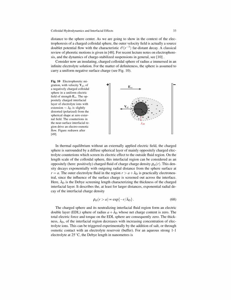
Colloidal Hydrodynamics and Interfacial Effects 33
distance to the sphere center. As we are going to show in the context of the elec-trophoresis of a charged colloidal sphere, the outer velocity field is actually a sourcedoublet potential flow with the characteristic O(r−3) far-distant decay. A classicalreview of phoretic motions is given in [48]. For recent lecture notes on electrophore-sis, and the dynamics of charge-stabilized suspensions in general, see [10] .
Consider now an insulating, charged colloidal sphere of radius a immersed in aninfinite electrolyte solution. For the matter of definiteness, the sphere is assumed tocarry a uniform negative surface charge (see Fig. 10).
Fig. 10 Electrophoretic mi-gration, with velocity Vel, ofa negatively charged colloidalsphere in a uniform electricfield of strength E∞. The op-positely charged interfaciallayer of electrolyte ions withextension ∼ λD is slightlydistorted (polarized) from thespherical shape at zero exter-nal field. The counterions inthe near-surface interfacial re-gion drive an electro-osmoticflow. Figure redrawn after[49].
-
- -- ----
------
--- -
----
- ++++
+
++++
++
+++++
+
+
+
+
+ _
In thermal equilibrium without an externally applied electric field, the chargedsphere is surrounded by a diffuse spherical layer of mainly oppositely charged elec-trolyte counterions which screen its electric effect to the outside fluid region. On thelength scale of the colloidal sphere, this interfacial region can be considered as anoppositely (here: positively) charged fluid of charge charge density ρel(r). This den-sity decays exponentially with outgoing radial distance from the sphere surface atr = a. The outer electrolyte fluid in the region r > a+λD is practically electroneu-tral, since the influence of the surface charge is screened out across the interface.Here, λD is the Debye screening length characterizing the thickness of the chargedinterfacial layer. It describes the, at least for larger distances, exponential radial de-cay of the interfacial charge density
ρel(r > a) ∝ exp−r/λD . (68)
The charged sphere and its neutralizing interfacial fluid region form an electricdouble layer (EDL) sphere of radius a+λD whose net charge content is zero. Thetotal electric force and torque on the EDL sphere are consequently zero. The thick-ness, λD, of the interfacial region decreases with increasing concentration of elec-trolyte ions. This can be triggered experimentally by the addition of salt, or throughosmotic contact with an electrolyte reservoir (buffer). For an aqueous strong 1-1electrolyte at 25 C, the Debye length in nanometres is
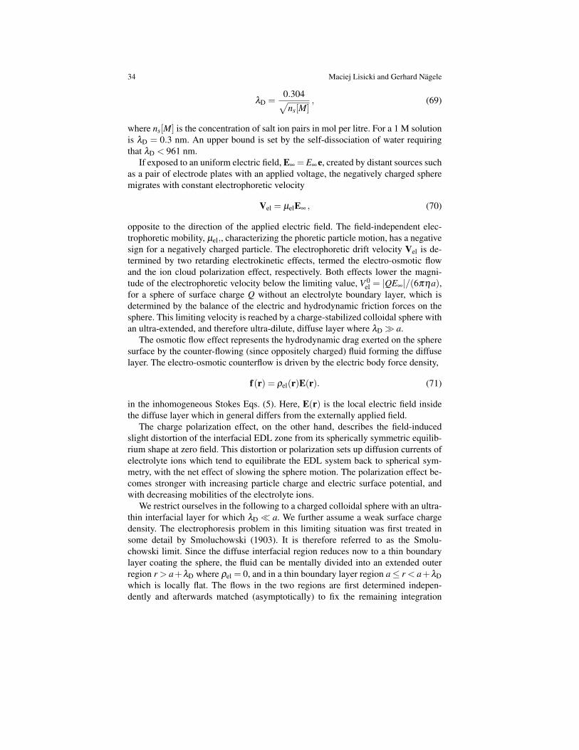
34 Maciej Lisicki and Gerhard Nagele
λD =0.304√
ns[M], (69)
where ns[M] is the concentration of salt ion pairs in mol per litre. For a 1 M solutionis λD = 0.3 nm. An upper bound is set by the self-dissociation of water requiringthat λD < 961 nm.
If exposed to an uniform electric field, E∞ = E∞ e, created by distant sources suchas a pair of electrode plates with an applied voltage, the negatively charged spheremigrates with constant electrophoretic velocity
Vel = µelE∞ , (70)
opposite to the direction of the applied electric field. The field-independent elec-trophoretic mobility, µel,, characterizing the phoretic particle motion, has a negativesign for a negatively charged particle. The electrophoretic drift velocity Vel is de-termined by two retarding electrokinetic effects, termed the electro-osmotic flowand the ion cloud polarization effect, respectively. Both effects lower the magni-tude of the electrophoretic velocity below the limiting value, V 0
el = |QE∞|/(6πηa),for a sphere of surface charge Q without an electrolyte boundary layer, which isdetermined by the balance of the electric and hydrodynamic friction forces on thesphere. This limiting velocity is reached by a charge-stabilized colloidal sphere withan ultra-extended, and therefore ultra-dilute, diffuse layer where λD a.
The osmotic flow effect represents the hydrodynamic drag exerted on the spheresurface by the counter-flowing (since oppositely charged) fluid forming the diffuselayer. The electro-osmotic counterflow is driven by the electric body force density,
f(r) = ρel(r)E(r). (71)
in the inhomogeneous Stokes Eqs. (5). Here, E(r) is the local electric field insidethe diffuse layer which in general differs from the externally applied field.
The charge polarization effect, on the other hand, describes the field-inducedslight distortion of the interfacial EDL zone from its spherically symmetric equilib-rium shape at zero field. This distortion or polarization sets up diffusion currents ofelectrolyte ions which tend to equilibrate the EDL system back to spherical sym-metry, with the net effect of slowing the sphere motion. The polarization effect be-comes stronger with increasing particle charge and electric surface potential, andwith decreasing mobilities of the electrolyte ions.
We restrict ourselves in the following to a charged colloidal sphere with an ultra-thin interfacial layer for which λD a. We further assume a weak surface chargedensity. The electrophoresis problem in this limiting situation was first treated insome detail by Smoluchowski (1903). It is therefore referred to as the Smolu-chowski limit. Since the diffuse interfacial region reduces now to a thin boundarylayer coating the sphere, the fluid can be mentally divided into an extended outerregion r > a+λD where ρel = 0, and in a thin boundary layer region a≤ r < a+λDwhich is locally flat. The flows in the two regions are first determined indepen-dently and afterwards matched (asymptotically) to fix the remaining integration
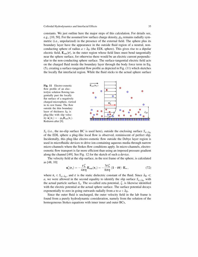
Colloidal Hydrodynamics and Interfacial Effects 35
constants. We just outline here the major steps of this calculation. For details see,e.g., [10, 50]. For the assumed low surface charge density, ρel remains radially sym-metric (i.e., unpolarized) in the presence of the external field. The sphere plus itsboundary layer have the appearance in the outside fluid region of a neutral, non-conducting sphere of radius a+λD (the EDL sphere). This gives rise to a dipolarelectric field, Eout(r), in the outer region whose field lines must bend tangentiallynear the sphere surface, for otherwise there would be an electric current perpendic-ular to the non-conducting sphere surface. The surface-tangential electric field actson the charged fluid inside the boundary layer through the body force term in Eq.(5), creating a surface-tangential flow profile as depicted in Fig. (11) which sketchesthe locally flat interfacial region. While the fluid sticks to the actual sphere surface
Fig. 11 Electro-osmoticflow profile of an elec-trolyte solution flowing tan-gentially past the locallyflat surface of a negativelycharged microsphere, viewedin its rest frame. The flowoutside the thin boundarylayer of thickness λD isplug-like with slip veloc-ity u′s(rs) = −µelEout(rs).Redrawn after [9].
++
++
+
+
+
++ +
+
+
++
+
+
-
-
-
-
-
-
-
-
++
+- -
-
-
+
+
++
+
Sa (i.e., the no-slip surface BC is used here), outside the enclosing surface Sa+λDof the EDL sphere a plug-like local flow is observed, reminiscent of perfect slip.Incidentally, this plug-like electro-osmotic flow outside the Debye layer region isused in microfluidic devices to drive ion-containing aqueous media through narrowmicro-channels where the Stokes flow conditions apply. In micro-channels, electro-osmotic flow transport is far more efficient than using an imposed pressure gradientalong the channel [49]. See Fig. 12 for the sketch of such a device.
The velocity field at the slip surface, in the rest frame of the sphere, is calculatedas [48, 10]
u′s(rs) =−εζ
4πηEout(rs) =−
3εζ
8πη(1− rr) ·E∞ , (72)
where rs ∈ Sa+λD , and ε is the static dielectric constant of the fluid. Since λD a, we were allowed in the second equality to identify the slip surface Sa+λD withthe actual particle surface Sa. The so-called zeta potential, ζ , is likewise identifiedwith the electric potential at the actual sphere surface. The surface potential decaysexponentially to zero in going outwards radially from a to a+λD.
Since the outer fluid is uncharged, the outer velocity field in the lab frame isfound from a purely hydrodynamic consideration, namely from the solution of thehomogeneous Stokes equations with inner inner and outer BCs,
36 Maciej Lisicki and Gerhard NageleElectro()(osmo,c(plug(flow(in(an(open(capillary(tube(
• Electroosmosis used in microfluid devices to drive aqueous media through narrow micro - channels where Low-Reynolds number fluid dynamics applies to
Anode& Cathode&
glass(wall&
U&
plug&flow&
+"""""""""+"""""""""&+"""""""""&+"""""""""&+"""""""""&+"""""""""&+&
+"""""""""+"""""""""&+"""""""""&+"""""""""&+""""""""""&+""""""""&+&
−"""""""""−""""""""&−"""""""""&−"""""""""&&−"""""""&−""""""""&−&
−"""""""""−""""""""&−"""""""""&−"""""""""&&−""""""""&−""""""""&−&
∞E
2h
3(
Fig. 12 Sketch of electro-osmotic plug flow in an open microcapillary tube with negativelycharged glass walls. The non-dissipative plug flow is driven by the field-induced migration ofcounterions accumulated in the thin Debye interfacial layer of thickness λD 2h at the glasswalls. In a tube closed at both ends, a pressure difference is created along the channel which drivesa Poiseuille-type backflow of fluid in the central region of the tube [49].
uout(rs) = Vel +u′s(rs) , uout(r→ ∞) = 0 . (73)
respectively, where rs ∈ Sa+λD ≈ Sa, and the sphere located momentarily at the co-ordinate frame origin. The electrophoretic velocity Vel is still unknown to this point.The boundary value problem has a unique flow solution if one demands in additionthe EDL sphere to be force- and torque free, in accord with its overall electroneu-trallity.
To determine uout using the singularity method, we notice first that the Stokesletand Rotlet are ruled out as flow contributions since they would result in a non-zerodrag force and torque. Therefore, we use the ansatz,
uout(r) = c3a3DS(r;e) . (74)
for the out flow in the lab frame, with a source doublet in direction e of the ap-plied electric field. With this ansatz, the inner and outer BCs are fulfilled with c3determined as c3 = εζ E∞/(8πη), and the electrophoretic velocity as
Vel = µel E∞ , µel =εζ
4πη, (75)
respectively. The so-called Smoluchowski electrophoretic mobility µel scales lin-early with the electric zeta potential, and it is independent of the particle radius. Theouter velocity field in the lab frame is thus
uout(r) =12
(ar
)3[3rr−1] ·Vel = µel Eout(r)+Vel . (76)
In the second equality, we have expressed the velocity field in terms of the outerelectric dipole field.
Being an incompressible potential flow field, uout fulfils ∆uout = 0 with ∇pout =0, so that the outer pressure field is uniform. The source doublet streamlines of the
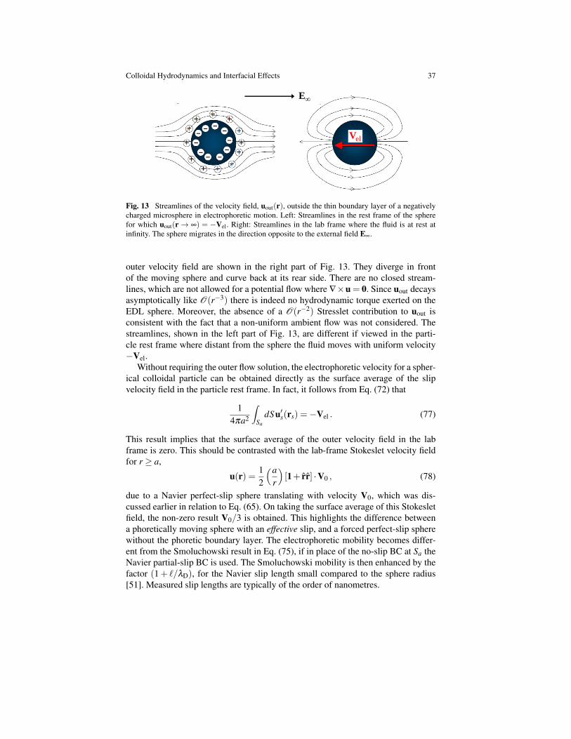
Colloidal Hydrodynamics and Interfacial Effects 37
elV
E
Fig. 13 Streamlines of the velocity field, uout(r), outside the thin boundary layer of a negativelycharged microsphere in electrophoretic motion. Left: Streamlines in the rest frame of the spherefor which uout(r→ ∞) = −Vel. Right: Streamlines in the lab frame where the fluid is at rest atinfinity. The sphere migrates in the direction opposite to the external field E∞.
outer velocity field are shown in the right part of Fig. 13. They diverge in frontof the moving sphere and curve back at its rear side. There are no closed stream-lines, which are not allowed for a potential flow where ∇×u = 0. Since uout decaysasymptotically like O(r−3) there is indeed no hydrodynamic torque exerted on theEDL sphere. Moreover, the absence of a O(r−2) Stresslet contribution to uout isconsistent with the fact that a non-uniform ambient flow was not considered. Thestreamlines, shown in the left part of Fig. 13, are different if viewed in the parti-cle rest frame where distant from the sphere the fluid moves with uniform velocity−Vel.
Without requiring the outer flow solution, the electrophoretic velocity for a spher-ical colloidal particle can be obtained directly as the surface average of the slipvelocity field in the particle rest frame. In fact, it follows from Eq. (72) that
14πa2
∫Sa
dSu′s(rs) =−Vel . (77)
This result implies that the surface average of the outer velocity field in the labframe is zero. This should be contrasted with the lab-frame Stokeslet velocity fieldfor r ≥ a,
u(r) =12
(ar
)[1+ rr] ·V0 , (78)
due to a Navier perfect-slip sphere translating with velocity V0, which was dis-cussed earlier in relation to Eq. (65). On taking the surface average of this Stokesletfield, the non-zero result V0/3 is obtained. This highlights the difference betweena phoretically moving sphere with an effective slip, and a forced perfect-slip spherewithout the phoretic boundary layer. The electrophoretic mobility becomes differ-ent from the Smoluchowski result in Eq. (75), if in place of the no-slip BC at Sa theNavier partial-slip BC is used. The Smoluchowski mobility is then enhanced by thefactor (1+ `/λD), for the Navier slip length small compared to the sphere radius[51]. Measured slip lengths are typically of the order of nanometres.
38 Maciej Lisicki and Gerhard Nagele
For the general case of a phoretically moving microsphere, it can be shown thatits drift velocity is given by the surface average [52, 53]
Vphor =−1
4πa2
∫Sa
dS µs(rs) [1− rr] ·∇φ(rs) , (79)
where φ stands likewise for the potential of the applied electric field, temperatureor solute concentration. Here, µs(rs) is a local surface mobility coefficient allowedto vary over the sphere surface. In our discussion of electrophoresis the potentialgradient and mobility are taken as constant, with the latter equal to (3/2)µel.
On recalling the steps which led to Eq. (75), one notices that owing to the localsurface flatness on the scale of λD, the inner boundary value problem for the in-terfacial region is independent of the global shape of the microparticle. Therefore,the second equality in Eq. (76) remains valid for arbitrarily shaped, non-conductingrigid particles, provided the local radius of curvature at all surface points is largecompared to λD. What varies with the particle shape is only the near-distance formof Eout(r). The latter is determined by the electrostatic boundary value problem of anon-conducting particle in an external field, with its field lines bending tangentiallyclose to the particle surface to satisfy the non-conductance condition. The crucialpoint here is that the explicit form of Eout(r) is not required for the determination ofthe electrophoretic mobility. In fact, on noting Eout→ E∞ and uout→ 0 for r→ ∞,the Smoluchowski mobility result in Eq. (75) is readily recovered from the secondequality in Eq. (76), but now for arbitrary particle shape and size, under the provisothat the particle has uniform surface zeta potential ζ . This remarkable result is sup-plemented by the likewise remarkable feature that the particle migrates phoreticallywithout rotating. This follows from the fact that the far-distant form of Eout(r) is adipolar electric field of O(r−3), independent of the particle shape. This in turn im-plies that uout(r) is a potential flow field with a likewise O(r−3) far-distance decay.Such a flow exerts no hydrodynamic torque on the particle which consequently isnon-rotating while translating.
However, the remarkable finding of shape-independent mobility has been ob-tained based on various restrictions. We quote here the most important ones: Firstly,the surface zeta potential is assumed to be weak enough for the polarization of thediffuse layer to be negligible, i.e. |ζ e| is small compared to kBT , with e denoting theelementary charge. Secondly, the diffuse boundary layer must be very thin. More-over, the applied electric field should be uniform on the scale of the particle size,and the small excluded volume of the electrolyte ions should not matter. The ionsmust be monovalent, and the dielectric constant and electrolyte viscosity should notchange across the boundary layer. See [54] for a quantitative theory for the concen-tration dependence of the electrolyte viscosity.
For an isolated charge-stabilized sphere, surface uniformity of zeta potential andsurface charge density go hand in hand. However, this is not the case for a non-spherical particle which has surface regions of varying curvature. A particle withuniform surface charge density has a larger zeta potential in the regions of highercurvature. This causes the particle to reorient while translating.
Colloidal Hydrodynamics and Interfacial Effects 39
We proceed with the interesting generalization that a force F = Fe co-linear withthe applied field is acting on the electrophoretically moving sphere. The sphere ve-locity V =V e and the flow for this situation can be constructed by the addition of aStokeslet field of strength F to the source doublet, i.e
u(r) =(a
r
)[1− rr]
(F
8πηa
)+
c3
2
(ar
)3[3 rr−1]
· e . (80)
The two conditions determining c3 and the sphere velocity are
u(±ae) = V
u(ar)−V = −32(1− rr) ·Vel . (81)
The first condition assures that the fluid velocity at the poles of the sphere agreeswith its velocity. The second condition demands the phoretic surface flow in therest frame of the sphere to be the same as in unforced electrophoresis. This is areasonable requirement since for negligible EDL polarization the local osmotic flowin the boundary layer does not depend on whether the sphere is forced or not. Toevaluate the second condition, one selects a unit vector r = e⊥ perpendicular to e.The results is
V = Vel +F
6πηa= µ
t0F +µelE∞
c3 = Vel−F
12πηa. (82)
The first equation expresses the expected linear superposition of the particle veloci-ties of the two problems of a phoretically moving sphere without body force, and aforced no-slip sphere without phoresis. It can be likewise formulated as a mobilityproblem for given forces F and eE∞. The second force contribution, however, is nota body force.
The sphere becomes stationary, with V = 0, when the body force is equal to
F =−(6πηa)Vel , (83)
i.e. equal to the hydrodynamic drag force on a no-slip and non-phoretic spheremoving with velocity Vel. Stationarity can be achieved experimentally, up to theinevitable undirected Brownian motion for smaller particles, using optical tweezers.The flow field of a stationary phoretic sphere is thus
u(r) =−34
(ar
)[1− rr]−
(ar
)3[3 rr−1]
·µelE∞ . (84)
The surface average of this velocity field yields µelE∞, which expresses again thebody-force independence of the surface osmotic flow.
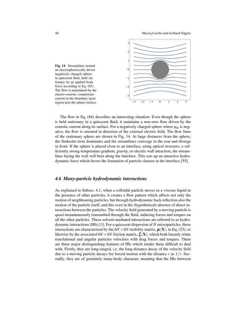
40 Maciej Lisicki and Gerhard Nagele
Fig. 14 Streamlines aroundan electrophoretically drivennegatively charged spherein quiescent fluid, held sta-tionary by an applied bodyforce according to Eq. (83).The flow is maintained by theelectro-osmotic counterionscurrent in the boundary layerregion near the sphere surface.
The flow in Eq. (84) describes an interesting situation: Even though the sphereis held stationary in a quiescent fluid, it maintains a non-zero flow driven by theosmotic current along its surface. For a negatively charged sphere where µel is neg-ative, the flow is oriented in direction of the external electric field. The flow linesof the stationary sphere are shown in Fig. 14. At large distances from the sphere,the Stokeslet term dominates and the streamlines converge in the rear and divergein front. If the sphere is placed close to an interface, using optical tweezers, a suf-ficiently strong temperature gradient, gravity, or electric wall attraction, the stream-lines facing the wall will bent along the interface. This sets up an attractive hydro-dynamic force which favors the formation of particle clusters at the interface [55].
4.6 Many-particle hydrodynamic interactions
As explained in Subsec. 4.1, when a colloidal particle moves in a viscous liquid inthe presence of other particles, it creates a flow pattern which affects not only themotion of neighbouring particles, but through hydrodynamic back reflection also themotion of the particle itself, and this even in the (hypothetical) absence of direct in-teractions between the particles. The velocity field generated by a moving particle isquasi-instantaneously transmitted through the fluid, inducing forces and torques onall the other particles. These solvent-mediated interactions are referred to as hydro-dynamic interactions (HIs) [1]. For a quiescent dispersion of N microparticles, theseinteractions are characterized by the 6N×6N mobility matrix, µµµ(X), in Eq. (23), orlikewise by the associated 6N×6N friction matrix, ζζζ (X), which both linearly relatetranslational and angular particles velocities with drag forces and torques. Thereare three major distinguishing features of HIs which render them difficult to dealwith. Firstly, they are long-ranged, i.e. the long-distance decay of the velocity fielddue to a moving particle decays for forced motion with the distance r as 1/r. Sec-ondly, they are of genuinely many-body character, meaning that the HIs between
Colloidal Hydrodynamics and Interfacial Effects 41
a pair of particles are changed through the presence of a third one in their vicin-ity. To account for the non-additivity requires the consideration of multiple flowreflections by neighbouring microparticles, with the reflections being responsiblefor the deviations of the exact HIs from the approximate form in terms of a su-perposition of pair contributions. The approximate pairwise additivity treatment ofthe HIs where flow reflections are disregarded altogether can be justified for dilutedispersions only, for conditions where all particles are mutually well separated onthe scale of their sizes. Non-pairwise additive higher-order HIs effects are importantin particular in the dynamics of concentrated dispersions. The third distinguishingfeature of the HIs is that, differently from direct interactions, they do not affect theequilibrium microstructure (i.e., the configurational distribution function Peq(X)), indispersions without external fields or imposed macroscopic flows. This is reflectedby the fact that owing to their interrelation with hydrodynamic friction forces, HIsare not derivable from a many-particle conservative potential energy function deter-mining the equilibrium distribution function.
Since diffusion transport properties of suspensions are expressible as configura-tional averages of certain tensor elements of µµµ(X), and since µµµ(X) is a key ingre-dient in the many-particle Smoluchowski and Stokes-Liouville equations governingthe evolution of the configurational distribution function P(X, t) of Brownian andnon-Brownian microparticles, respectively, it is essential to be able to calculate thismatrix for a many-particle system. Over the years, various numerical methods havebeen developed for this purpose, and a number of review articles [29, 37] and books[1, 14, 21] dealing with HIs are available.
If the microparticles are mutually well separated, with relative distances largecompared to their size, the flow induced by their motion can be regarded approxi-mately as originating from point forces concentrated at their centres. This liberatesone from the severe complications of having to invoke the prescribed hydrodynamicBCs simultaneously on the particle surfaces. The tensorial mobility coefficients de-scribing the linear relations between applied forces and resulting velocities are thenstraightforwardly approximated by the superposition of Stokeslets at the particlecentres according to (point-particles model)
µµµttii ≈ µ
t01 , (85)
µµµtti j ≈ T(Ri−R j) (86)
for i 6= j. Here, µ t0i is the single-particle translational mobility coefficient of particle
i, and 1 is the unit tensor. Only the leading-order long-distance behaviour of theflow field is included in the point-particles model, with the off-diagonal mobilitytensors decaying as r−1 in the inter-particle distance r. While the pairwise additivepoint-particles model is applicable to well-separated particles, it usually fails whenparticles are close to each other or to a confining wall, as indicated by the possibleviolation of the positive definiteness of the mobility matrix approximation in Eq.(85). At large concentrations and for smaller inter-particle distances, more refinedtheoretical methods and numerical schemes are required to account for the near-distance and non pairwise additive contributions to the HIs.
42 Maciej Lisicki and Gerhard Nagele
The next important step in going beyond the point-particles model is to accountfor the non-zero volumes of the particles while still maintaining the pairwise addi-tive single-particle flow superposition. For spherical no-slip particles this is referredto as the Rotne-Prager (RP) mobility matrix approximation [56], and with an appro-priate extension to overlapping no-slip spheres also as the Rotne-Prager-Yamakawa(RPY) approximation [57, 58]. The RP approximation is still pairwise additive, withthe RP mobility tensors exhibiting a long-distance decay of O(r−3). All the hydro-dynamic back reflections, which give rise to more steeply decaying flow field contri-butions of O(r−4), are hereby disregarded. The main merit of the RP approximation,in addition to its convenient simplicity, is that is leads to a translational mobility ma-trix approximation, µµµ tt,RP, which is positive definite for all physically allowed con-figurations of non-overlapping spheres. Moreover, µµµ tt,RP is an upper bound to theexact translational mobility matrix, µµµ tt , in the sense that b ·
(µµµ tt,RP−µµµ tt
)·b > 0 for
all non-zero 3N-dimensional vectors b and all allowed configurations. This prop-erty of the RP approximation can be used for constructing upper bounds to certaintransport properties of concentrated dispersion such as the (short-time) mean sedi-mentation velocity. The RP approximation can be profitably used for dilute to mod-erately concentrated dispersions of no-slip microspheres which strongly repel eachother over larger distances. Examples in case are like-charged colloidal particles,and lower-salinity aqueous solutions of globular proteins.
The derivation of the translational mobility matrix in RP approximation proceedsas follows: Consider first an isolated no-slip microsphere j of radius a in an infinitequiescent fluid, translating without rotation under the action of the force F j actingat its centre at R j. From Eq. (38), one notices that σσσ ·n = F j/(4πa2) is consistentwith the no-slip BC on the sphere surface, i.e. the surface shear stress in this specialsituation is constant. Consequently,
u(0)j (r) =
∫dS′T(r− r′) ·
F j
4πa2 =
(1+
a2
6∇
2)
T(r−R j) ·F j (87)
where for the second equality, the mean-value theorem for bi-harmonic functionshas been used [59], on recalling that ∇2∇2T(r) = 0 for all non-zero vectors r. Fromperforming the second-order differentiation, one verifies that u(0)
j (r) is equal to thevelocity field in Eq. (66) which we had obtained earlier using the singularity flowsolutions.
Consider next the incident flow, u(N−1)inc (r), created by the motion of (N − 1)
no-slip spheres at the position Ri of another sphere i. It should be noticed herethat u(N−1)
inc (r) is determined by the BCs on all N spheres, including the singled-out sphere i. In the RP treatment, the incident flow is crudely approximated by thesuperposition of the single-sphere flow fields,
u(N−1)inc (r)≈
N
∑j 6=i
u(0)j (r) . (88)
Colloidal Hydrodynamics and Interfacial Effects 43
In this incident flow field approximation, the (N−1) no-slip BCs are only approxi-mately fulfilled for configurations of mutually well separated spheres.
The velocity, Vi, of a no-slip microsphere i of radius a in an infinite fluid, sub-jected a force Fi and an incident flow field uinc(r), is given by the exact translationalFaxen law
Vi = µt0 Fi +
(1+
a2
6∇
2i
)uinc(Ri) , (89)
where µ t0 is the translational single-particle mobility of a no-slip sphere. The only
restriction on the form of the incident flow is that it has to be a Stokes flow solution,created by sources located outside the volume of sphere i. These sources could be,e.g., other microparticles or confining walls, whereby the wall influence can be de-scribed by an image system as discussed in the following section. A derivation ofthe present Faxen theorem is given, e.g., in [14, 35]. According to the Faxen theo-rem, freely advected, i.e. force- and torque-free, small particles can be used to traceout the streamlines caused by the motion of big ones. For an example, consider asmall tracer sphere i placed in the (incident) flow of, say, a phoretically moving bigsphere. Since on the small length scale a of the tracer the curvature contribution inEq. (89) described by the Laplacian can be neglected, one has
Vi ≈ uinc(r = Ri) (90)
for the velocity of the tracer dragged along in the flow field of the big particle.Small tracer tracer particles have been used experimentally, e.g., to visualize thethermophoretic quasi-slip flow around a big polystyrene or silica sphere near a sur-face, driven by a temperature gradient in the fluid oriented perpendicular to thesurface [60].
We use now the Faxen theorem to obtain the velocity of a no-slip sphere i ofradius a in the incident flow of (N− 1) other ones of equal radii, using the single-spheres flow superposition. The result is
Vi ≈ µt0 Fi +
N
∑j 6=i
(1+
a2
3∇
2i
)T(Ri−R j) ·F j , (91)
where ∇2i ∇2
j T(Ri−R j) = 0 for i 6= j has been used in the derivation. The transla-tional mobilities in the RP approximation follow readily from this result as
µµµtt,RPii = µ
t01 (92)
µµµtt,RPi j = µ
t0
[34
(ar
)(111+ rr)+
12
(ar
)3(111−3rr)
](93)
with r = Ri−R j. The positive definiteness of the RP translational mobility matrixcan be shown, e.g., using the double surface integral representation of its tensorelements,
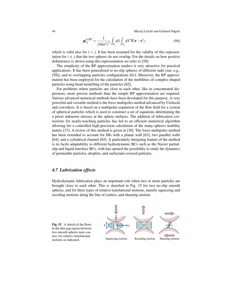
44 Maciej Lisicki and Gerhard Nagele
µµµtt,RPi j =
1
(4πa2)2
∫Si
dS∫
S j
dS′T(r− r′) , (94)
which is valid also for i = j. It has been assumed for the validity of this represen-tation for i 6= j that the two spheres do not overlap. For the details on how positivedefiniteness is shown using this representation we refer to [58].
The simplicity of the RP approximation renders it very attractive for practicalapplications. It has been generalized to no-slip spheres of different radii (see, e.g.,[58]), and to overlapping particles configurations [61]. Moreover, the RP approxi-mation has been employed for the calculation of the mobilities of complex-shapedparticles using bead-modelling of the particles [62].
For problems where particles are close to each other, like in concentrated dis-persions, more precise methods than the simple RP approximation are required.Various advanced numerical methods have been developed for this purpose. A verypowerful and versatile method is the force multipoles method advanced by Cichockiand coworkers. It is based on a multipolar expansion of the flow field for a systemof spherical particles which is used to construct a set of equations determining thea priori unknown stresses at the sphere surfaces. The addition of lubrication cor-rections for nearly-touching particles has led to an efficient numerical algorithmallowing for a controlled high-precision calculation of the many-spheres mobilitymatrix [37]. A review of this method is given in [38]. The force multipoles methodhas been extended to account for HIs with a planar wall [63], two parallel walls[64], and a cylindrical channel [65]. A particularly intriguing feature of the methodis its facile adaptability to different hydrodynamic BCs such as the Navier partial-slip and liquid interface BCs, with has opened the possibility to study the dynamicsof permeable particles, droplets, and surfactant-covered particles.
4.7 Lubrication effects
Hydrodynamic lubrication plays an important role when two or more particles arebrought close to each other. This is sketched in Fig. 15 for two no-slip smoothspheres, and for three types of relative translational motions, namely squeezing andreceding motions along the line of centres, and shearing motion.
Fig. 15 A sketch of the flowsin the thin gap region betweentwo smooth spheres near con-tact, for relative translationalmotions as indicated.
h
z
Squeezing motion Receding motion Shearing motion
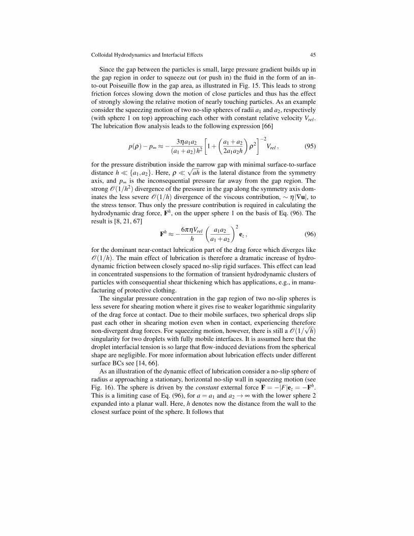
Colloidal Hydrodynamics and Interfacial Effects 45
Since the gap between the particles is small, large pressure gradient builds up inthe gap region in order to squeeze out (or push in) the fluid in the form of an in-to-out Poiseuille flow in the gap area, as illustrated in Fig. 15. This leads to strongfriction forces slowing down the motion of close particles and thus has the effectof strongly slowing the relative motion of nearly touching particles. As an exampleconsider the squeezing motion of two no-slip spheres of radii a1 and a2, respectively(with sphere 1 on top) approaching each other with constant relative velocity Vrel .The lubrication flow analysis leads to the following expression [66]
p(ρ)− p∞ ≈−3ηa1a2
(a1 +a2)h2
[1+(
a1 +a2
2a1a2h
)ρ
2]−2
Vrel , (95)
for the pressure distribution inside the narrow gap with minimal surface-to-surfacedistance h a1,a2. Here, ρ
√ah is the lateral distance from the symmetry
axis, and p∞ is the inconsequential pressure far away from the gap region. Thestrong O(1/h2) divergence of the pressure in the gap along the symmetry axis dom-inates the less severe O(1/h) divergence of the viscous contribution, ∼ η |∇u|, tothe stress tensor. Thus only the pressure contribution is required in calculating thehydrodynamic drag force, Fh, on the upper sphere 1 on the basis of Eq. (96). Theresult is [8, 21, 67]
Fh ≈−6πηVrel
h
(a1a2
a1 +a2
)2
ez , (96)
for the dominant near-contact lubrication part of the drag force which diverges likeO(1/h). The main effect of lubrication is therefore a dramatic increase of hydro-dynamic friction between closely spaced no-slip rigid surfaces. This effect can leadin concentrated suspensions to the formation of transient hydrodynamic clusters ofparticles with consequential shear thickening which has applications, e.g., in manu-facturing of protective clothing.
The singular pressure concentration in the gap region of two no-slip spheres isless severe for shearing motion where it gives rise to weaker logarithmic singularityof the drag force at contact. Due to their mobile surfaces, two spherical drops slippast each other in shearing motion even when in contact, experiencing thereforenon-divergent drag forces. For squeezing motion, however, there is still a O(1/
√h)
singularity for two droplets with fully mobile interfaces. It is assumed here that thedroplet interfacial tension is so large that flow-induced deviations from the sphericalshape are negligible. For more information about lubrication effects under differentsurface BCs see [14, 66].
As an illustration of the dynamic effect of lubrication consider a no-slip sphere ofradius a approaching a stationary, horizontal no-slip wall in squeezing motion (seeFig. 16). The sphere is driven by the constant external force F = −|F |ez = −Fh.This is a limiting case of Eq. (96), for a = a1 and a2→ ∞ with the lower sphere 2expanded into a planar wall. Here, h denotes now the distance from the wall to theclosest surface point of the sphere. It follows that
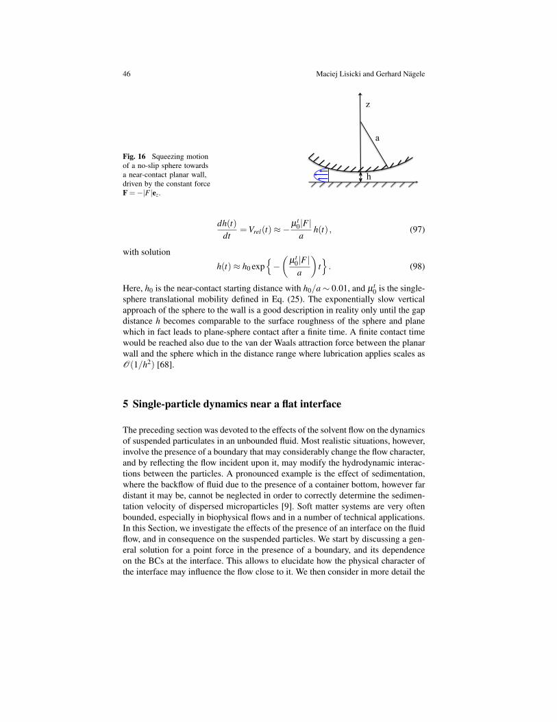
46 Maciej Lisicki and Gerhard Nagele
Fig. 16 Squeezing motionof a no-slip sphere towardsa near-contact planar wall,driven by the constant forceF =−|F |ez.
a
z
h
dh(t)dt
=Vrel(t)≈−µ t
0|F |a
h(t) , (97)
with solution
h(t)≈ h0 exp−(
µ t0|F |a
)t. (98)
Here, h0 is the near-contact starting distance with h0/a∼ 0.01, and µ t0 is the single-
sphere translational mobility defined in Eq. (25). The exponentially slow verticalapproach of the sphere to the wall is a good description in reality only until the gapdistance h becomes comparable to the surface roughness of the sphere and planewhich in fact leads to plane-sphere contact after a finite time. A finite contact timewould be reached also due to the van der Waals attraction force between the planarwall and the sphere which in the distance range where lubrication applies scales asO(1/h2) [68].
5 Single-particle dynamics near a flat interface
The preceding section was devoted to the effects of the solvent flow on the dynamicsof suspended particulates in an unbounded fluid. Most realistic situations, however,involve the presence of a boundary that may considerably change the flow character,and by reflecting the flow incident upon it, may modify the hydrodynamic interac-tions between the particles. A pronounced example is the effect of sedimentation,where the backflow of fluid due to the presence of a container bottom, however fardistant it may be, cannot be neglected in order to correctly determine the sedimen-tation velocity of dispersed microparticles [9]. Soft matter systems are very oftenbounded, especially in biophysical flows and in a number of technical applications.In this Section, we investigate the effects of the presence of an interface on the fluidflow, and in consequence on the suspended particles. We start by discussing a gen-eral solution for a point force in the presence of a boundary, and its dependenceon the BCs at the interface. This allows to elucidate how the physical character ofthe interface may influence the flow close to it. We then consider in more detail the
Colloidal Hydrodynamics and Interfacial Effects 47
motion of an isolated spherical particle close to a wall, with the BCs at the particlesurface and lubrication effects taken into account. We discuss the commonly usedapproximations for the mobility of a microsphere near a no-slip wall, and presentexamples of experimental techniques capable of grasping the dynamic behaviour.Finally, we explore the motion of flexible particles and the effect of deformableboundaries, in situations where the elasticity of the surface or particles may not beneglected.
5.1 Point force near an interface
To demonstrate the effects of partial confinement on the hydrodynamics of a sin-gle particle, we will show explicit solutions for the velocity fields for a point forceacting on a fluid bounded by a planar free surface, and a planar no-slip wall. Theseare limiting cases for a point-force near a planar liquid-liquid interface, in the limitthat the viscosity ratio, λ = η1/η2, is reaching infinity and zero, respectively. Thepoint force F is located at the point r0 = (x0,y0,h) in the upper half space at verticaldistance h > 0 above the (x− y) interface at z = 0. Searched for is the flow fieldu(r) in the upper half space z≥ 0. We take advantage of the linearity of the Stokesequations to construct the flow field using the method of images. Akin to electro-statics [36], a number of hydrodynamic problems of higher symmetry can be solvedby this elegant method. In this method, the fluid in the upper half-space of viscosityη = η1 is mentally extended into the lower half-space, with the BCs imposed by thetaken-out interface now accounted for in conjunction with the Stokeslet at r0 by animage system of elemental singularity solutions placed at appropriate positions inthe lower half-space. The flow field constructed in this way is in the upper half-spaceidentical to the original flow problem where the interface is present.
For a point force in front of a planar liquid-liquid interface, the image systemmultipoles are all located at the same image point
r∗0 = Pz · r0 = (x0,y0,−h) . (99)
HerePz = 1− ezez (100)
is the (x− y) plane reflection matrix. This matrix acting on an arbitrary vector turnsthe z-component of this vector into its negative.
Free surface: We explain the image method first for the simplest case of a Stokesletabove a free surface, e.g., a non-contaminated air-water interface or a Navier perfect-slip wall. The BCs for such an interface is that the surface flow has only an in-planetangential component, and that there is no tangential stress across the interface. Thisis expressed by Eq. (17) in the limit that the viscosity, η2, of the fluid in the lowerhalf space vanishes, that is for λ→ 0. We shall assume the free surface not to deform
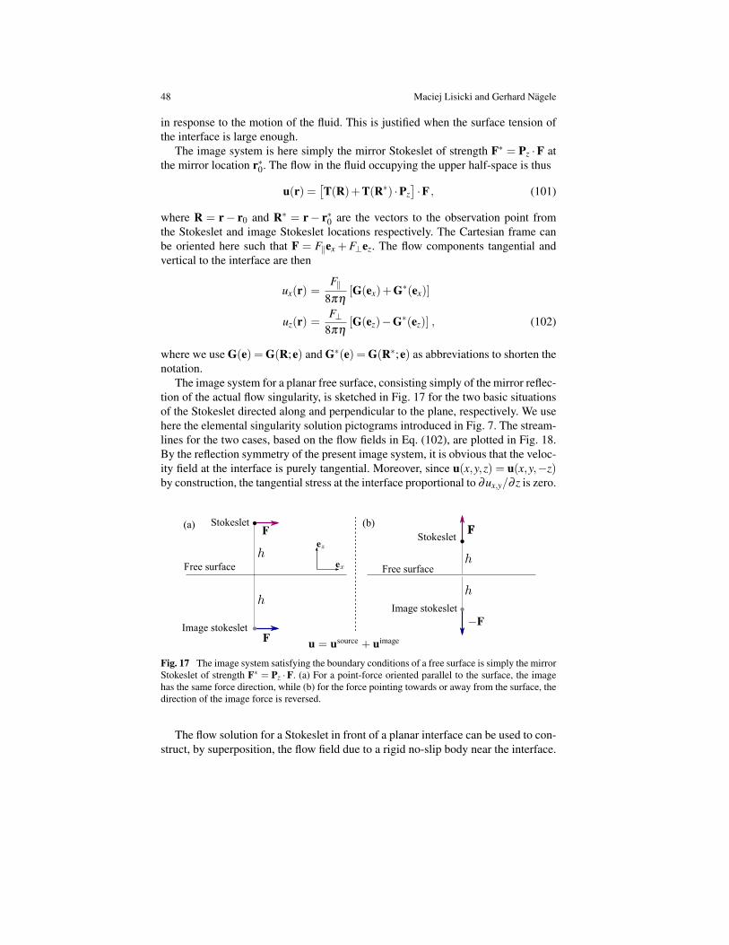
48 Maciej Lisicki and Gerhard Nagele
in response to the motion of the fluid. This is justified when the surface tension ofthe interface is large enough.
The image system is here simply the mirror Stokeslet of strength F∗ = Pz ·F atthe mirror location r∗0. The flow in the fluid occupying the upper half-space is thus
u(r) =[T(R)+T(R∗) ·Pz
]·F , (101)
where R = r− r0 and R∗ = r− r∗0 are the vectors to the observation point fromthe Stokeslet and image Stokeslet locations respectively. The Cartesian frame canbe oriented here such that F = F‖ex +F⊥ez. The flow components tangential andvertical to the interface are then
ux(r) =F‖
8πη[G(ex)+G∗(ex)]
uz(r) =F⊥
8πη[G(ez)−G∗(ez)] , (102)
where we use G(e) = G(R;e) and G∗(e) = G(R∗;e) as abbreviations to shorten thenotation.
The image system for a planar free surface, consisting simply of the mirror reflec-tion of the actual flow singularity, is sketched in Fig. 17 for the two basic situationsof the Stokeslet directed along and perpendicular to the plane, respectively. We usehere the elemental singularity solution pictograms introduced in Fig. 7. The stream-lines for the two cases, based on the flow fields in Eq. (102), are plotted in Fig. 18.By the reflection symmetry of the present image system, it is obvious that the veloc-ity field at the interface is purely tangential. Moreover, since u(x,y,z) = u(x,y,−z)by construction, the tangential stress at the interface proportional to ∂ux,y/∂ z is zero.
Free surface
Stokeslet
Image stokeslet
(b)
Free surface
Stokeslet
Image stokeslet
(a)
Fig. 17 The image system satisfying the boundary conditions of a free surface is simply the mirrorStokeslet of strength F∗ = Pz ·F. (a) For a point-force oriented parallel to the surface, the imagehas the same force direction, while (b) for the force pointing towards or away from the surface, thedirection of the image force is reversed.
The flow solution for a Stokeslet in front of a planar interface can be used to con-struct, by superposition, the flow field due to a rigid no-slip body near the interface.
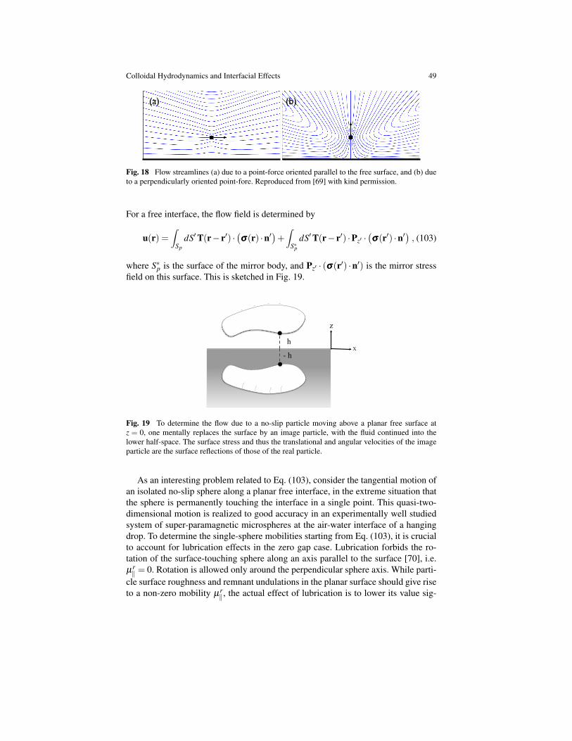
Colloidal Hydrodynamics and Interfacial Effects 49
(a) (b)
Fig. 18 Flow streamlines (a) due to a point-force oriented parallel to the free surface, and (b) dueto a perpendicularly oriented point-fore. Reproduced from [69] with kind permission.
For a free interface, the flow field is determined by
u(r) =∫
Sp
dS′T(r− r′) ·(σσσ(r) ·n′
)+∫
S∗pdS′T(r− r′) ·Pz′ ·
(σσσ(r′) ·n′
), (103)
where S∗p is the surface of the mirror body, and Pz′ · (σσσ(r′) ·n′) is the mirror stressfield on this surface. This is sketched in Fig. 19.
h
- h
z
X
Fig. 19 To determine the flow due to a no-slip particle moving above a planar free surface atz = 0, one mentally replaces the surface by an image particle, with the fluid continued into thelower half-space. The surface stress and thus the translational and angular velocities of the imageparticle are the surface reflections of those of the real particle.
As an interesting problem related to Eq. (103), consider the tangential motion ofan isolated no-slip sphere along a planar free interface, in the extreme situation thatthe sphere is permanently touching the interface in a single point. This quasi-two-dimensional motion is realized to good accuracy in an experimentally well studiedsystem of super-paramagnetic microspheres at the air-water interface of a hangingdrop. To determine the single-sphere mobilities starting from Eq. (103), it is crucialto account for lubrication effects in the zero gap case. Lubrication forbids the ro-tation of the surface-touching sphere along an axis parallel to the surface [70], i.e.µr‖ = 0. Rotation is allowed only around the perpendicular sphere axis. While parti-
cle surface roughness and remnant undulations in the planar surface should give riseto a non-zero mobility µr
‖, the actual effect of lubrication is to lower its value sig-
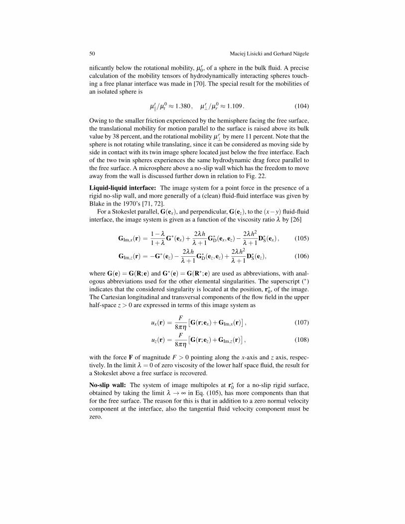
50 Maciej Lisicki and Gerhard Nagele
nificantly below the rotational mobility, µr0, of a sphere in the bulk fluid. A precise
calculation of the mobility tensors of hydrodynamically interacting spheres touch-ing a free planar interface was made in [70]. The special result for the mobilities ofan isolated sphere is
µt‖/µ
0t ≈ 1.380 , µ
r⊥/µ
0r ≈ 1.109 . (104)
Owing to the smaller friction experienced by the hemisphere facing the free surface,the translational mobility for motion parallel to the surface is raised above its bulkvalue by 38 percent, and the rotational mobility µr
⊥ by mere 11 percent. Note that thesphere is not rotating while translating, since it can be considered as moving side byside in contact with its twin image sphere located just below the free interface. Eachof the two twin spheres experiences the same hydrodynamic drag force parallel tothe free surface. A microsphere above a no-slip wall which has the freedom to moveaway from the wall is discussed further down in relation to Fig. 22.
Liquid-liquid interface: The image system for a point force in the presence of arigid no-slip wall, and more generally of a (clean) fluid-fluid interface was given byBlake in the 1970’s [71, 72].
For a Stokeslet parallel, G(ex), and perpendicular, G(ez), to the (x−y) fluid-fluidinterface, the image system is given as a function of the viscosity ratio λ by [26]
GIm,x(r) =1−λ
1+λG∗(ex)+
2λhλ +1
G∗D(ex,ez)−2λh2
λ +1D∗S(ex) , (105)
GIm,z(r) = −G∗(ez)−2λh
λ +1G∗D(ez,ez)+
2λh2
λ +1D∗S(ez), (106)
where G(e) = G(R;e) and G∗(e) = G(R∗;e) are used as abbreviations, with anal-ogous abbreviations used for the other elemental singularities. The superscript (∗)indicates that the considered singularity is located at the position, r∗0, of the image.The Cartesian longitudinal and transversal components of the flow field in the upperhalf-space z > 0 are expressed in terms of this image system as
ux(r) =F
8πη
[G(r;ex)+GIm,x(r)
], (107)
uz(r) =F
8πη
[G(r;ez)+GIm,z(r)
], (108)
with the force F of magnitude F > 0 pointing along the x-axis and z axis, respec-tively. In the limit λ = 0 of zero viscosity of the lower half space fluid, the result fora Stokeslet above a free surface is recovered.
No-slip wall: The system of image multipoles at r∗0 for a no-slip rigid surface,obtained by taking the limit λ → ∞ in Eq. (105), has more components than thatfor the free surface. The reason for this is that in addition to a zero normal velocitycomponent at the interface, also the tangential fluid velocity component must bezero.
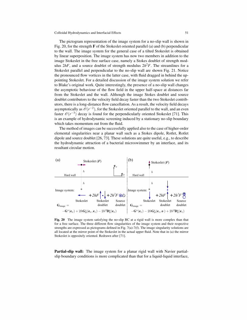
Colloidal Hydrodynamics and Interfacial Effects 51
The pictogram representation of the image system for a no-slip wall is shown inFig. 20, for the strength F of the Stokeslet oriented parallel (a) and (b) perpendicularto the wall. The image system for the general case of a tilted Stokeslet is obtainedby linear superposition. The image system has now two members in addition to theimage Stokeslet in the free surface case, namely a Stokes doublet of strength mod-ulus 2hF , and a source doublet of strength modulus 2h2F . The streamlines for aStokeslet parallel and perpendicular to the no-slip wall are shown Fig. 21. Noticethe pronounced flow vortices in the latter case, with fluid dragged in behind the up-pointing Stokeslet. For a detailed discussion of the image system solution we referto Blake’s original work. Quite interestingly, the presence of a no-slip wall changesthe asymptotic behaviour of the flow field in the upper half-space at distances farfrom the Stokeslet and the wall. Although the image Stokes doublet and sourcedoublet contributors to the velocity field decay faster than the two Stokeslet contrib-utors, there is a long-distance flow cancellation. As a result, the velocity field decaysasymptotically as O(r−2), for the Stokeslet oriented parallel to the wall, and an evenfaster O(r−3) decay is found for the perpendicularly oriented Stokeslet [71]. Thisis an example of hydrodynamic screening induced by a stationary no-slip boundarywhich takes momentum out from the fluid.
The method of images can be successfully applied also to the case of higher-orderelemental singularities near a planar wall such as a Stokes dipole, Rotlet, Rotletdipole and source doublet [26, 73]. These solutions are quite useful, e.g., to describethe hydrodynamic attraction of a bacterial microswimmer by an interface, and itsresultant circular motion.
Stokeslet (F)
+2hF
Stokeslet (F)
Stokeslet
Image system:
Stokeslet
doublet
Source
doublet
Hard wall Hard wall
(a) (b)
Image system:
+2h2F
Source
doublet
+2hF
Stokeslet
doublet
Stokeslet
+2h2F
Fig. 20 The image system satisfying the no-slip BC at a rigid wall is more complex than thatfor a free surface. The three different flow singularities of the image system and their respectivestrengths are expressed as pictograms defined in Fig. 7(a)-7(f). The image singularity solutions areall located at the mirror point of the Stokeslet in the actual upper fluid. Note that in (a) the mirrorStokeslet is oppositely oriented. Redrawn after [71].
Partial-slip wall: The image system for a planar rigid wall with Navier partial-slip boundary conditions is more complicated than that for a liquid-liquid interface,
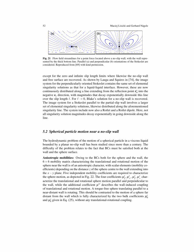
52 Maciej Lisicki and Gerhard Nagele
(a) (b)
Fig. 21 Flow field streamlines for a point force located above a no-slip wall, with the wall repre-sented by the thick bottom line. Parallel (a) and perpendicular (b) orientations of the Stokeslet areconsidered. Reproduced from [69] with kind permission.
except for the zero and infinite slip length limits where likewise the no-slip walland free surface are recovered. As shown by Lauga and Squires in [74], the imagesystem for the perpendicularly oriented Stokeslet contains the same set of elementalsingularity solutions as that for a liquid-liquid interface. However, these are nowcontinuously distributed along a line extending from the reflection point r∗0 into thenegative ez direction, with magnitudes that decay exponentially downside this lineover the slip length `. For `→ 0, Blake’s solution for a no-slip wall is recovered.The image system for a Stokeslet parallel to the partial-slip wall involves a largerset of elemental singularity solutions, likewise distributed along the aforementionedsingularity line. The system include now also a Rotlet and a Rotlet dipole. Here, notall singularity solution magnitudes decay exponentially in going downside along theline.
5.2 Spherical particle motion near a no-slip wall
The hydrodynamic problem of the motion of a spherical particle in a viscous liquidbounded by a planar no-slip wall has been studied since more than a century. Thedifficulty of the problem relates to the fact that BCs must be satisfied both at thewall and the sphere surface.
Anisotropic mobilities: Owing to the BCs both for the sphere and the wall, the6× 6 mobility matrix characterizing the translational and rotational motion of thesphere near the wall is of an anisotropic character, with scalar elements (mobility co-efficients) depending on the distance z of the sphere centre to the wall extending intothe x− y plane. Five independent mobility coefficients are required to characterizethe sphere motion, as depicted in Fig. 22. The four coefficients µ t
‖, µ t⊥, µr
‖, µr⊥ char-
acterize the translational and rotational sphere motion parallel and perpendicular tothe wall, while the additional coefficient µ tr describes the wall-induced couplingof translational and rotational motion. A torque-free sphere translating parallel to anear-distant wall is rotating. This should be contrasted to the motion of a sphere fardistant from the wall which is fully characterized by the two bulk coefficients µ t
0and µr
0 given in Eq. (25), without any translational-rotational coupling.
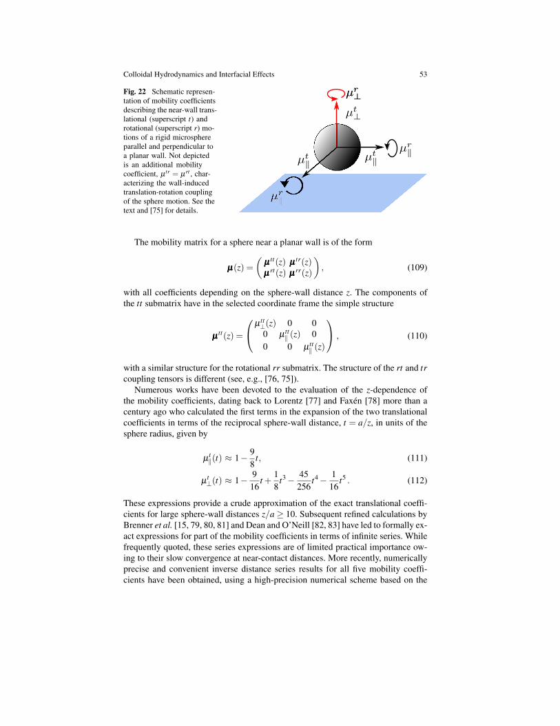
Colloidal Hydrodynamics and Interfacial Effects 53
Fig. 22 Schematic represen-tation of mobility coefficientsdescribing the near-wall trans-lational (superscript t) androtational (superscript r) mo-tions of a rigid microsphereparallel and perpendicular toa planar wall. Not depictedis an additional mobilitycoefficient, µ tr = µrt , char-acterizing the wall-inducedtranslation-rotation couplingof the sphere motion. See thetext and [75] for details.
The mobility matrix for a sphere near a planar wall is of the form
µµµ(z) =(
µµµ tt(z) µµµ tr(z)µµµrt(z) µµµrr(z)
), (109)
with all coefficients depending on the sphere-wall distance z. The components ofthe tt submatrix have in the selected coordinate frame the simple structure
µµµtt(z) =
µ tt⊥(z) 0 00 µ tt
‖ (z) 00 0 µ tt
‖ (z)
, (110)
with a similar structure for the rotational rr submatrix. The structure of the rt and trcoupling tensors is different (see, e.g., [76, 75]).
Numerous works have been devoted to the evaluation of the z-dependence ofthe mobility coefficients, dating back to Lorentz [77] and Faxen [78] more than acentury ago who calculated the first terms in the expansion of the two translationalcoefficients in terms of the reciprocal sphere-wall distance, t = a/z, in units of thesphere radius, given by
µt‖(t) ≈ 1− 9
8t, (111)
µt⊥(t) ≈ 1− 9
16t +
18
t3− 45256
t4− 116
t5 . (112)
These expressions provide a crude approximation of the exact translational coeffi-cients for large sphere-wall distances z/a ≥ 10. Subsequent refined calculations byBrenner et al. [15, 79, 80, 81] and Dean and O’Neill [82, 83] have led to formally ex-act expressions for part of the mobility coefficients in terms of infinite series. Whilefrequently quoted, these series expressions are of limited practical importance ow-ing to their slow convergence at near-contact distances. More recently, numericallyprecise and convenient inverse distance series results for all five mobility coeffi-cients have been obtained, using a high-precision numerical scheme based on the
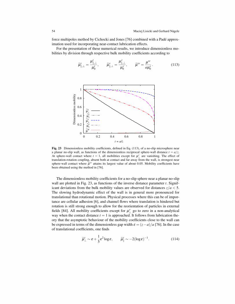
54 Maciej Lisicki and Gerhard Nagele
force multipoles method by Cichocki and Jones [76] combined with a Pade approx-imation used for incorporating near-contact lubrication effects.
For the presentation of these numerical results, we introduce dimensionless mo-bilities by division through respective bulk mobility coefficients according to
µt‖,⊥ =
µ t‖,⊥µ t
0, µ
r‖,⊥ =
µr‖,⊥µr
0, µ
tr =µ tr
aµr0. (113)
0
0.2
0.4
0.6
0.8
1
0 0.2 0.4 0.6 0.8 1
Dim
ensi
onle
ss m
obil
ity
t = a/z
µ~t
⊥
µ~t
||
µ~r
⊥
µ~r
||
µ~tr
Fig. 23 Dimensionless mobility coefficients, defined in Eq. (113), of a no-slip microsphere neara planar no-slip wall, as functions of the dimensionless reciprocal sphere-wall distance t = a/z.At sphere-wall contact where t = 1, all mobilities except for µr
⊥ are vanishing. The effect oftranslation-rotation coupling, absent both at contact and far away from the wall, is strongest nearsphere-wall contact where µ tr attains its largest value of about 0.05. Mobility coefficients havebeen obtained using the method in [76].
The dimensionless mobility coefficients for a no-slip sphere near a planar no-slipwall are plotted in Fig. 23, as functions of the inverse distance parameter t. Signif-icant deviations from the bulk mobility values are observed for distances z/a < 5.The slowing hydrodynamic effect of the wall is in general more pronounced fortranslational than rotational motion. Physical processes where this can be of impor-tance are cellular adhesion [6], and channel flows where translation is hindered butrotation is still strong enough to allow for the reorientation of particles in externalfields [84]. All mobility coefficients except for µr
⊥ go to zero in a non-analyticalway when the contact distance t = 1 is approached. It follows from lubrication the-ory that the asymptotic behaviour of the mobility coefficients close to the wall canbe expressed in terms of the dimensionless gap width ε = (z−a)/a [76]. In the caseof translational coefficients, one finds
µt⊥ ∼ ε +
15
ε2 logε, µ
t‖ ∼−2(logε)−1. (114)
Colloidal Hydrodynamics and Interfacial Effects 55
Wall lubrication effects imply also that µr‖(t → 1) = 0, whereas the sphere rotation
with the angular velocity oriented perpendicular to the wall is possible even at con-tact where the related mobility coefficient µr
⊥ is reduced by about 18 percent belowthe isotropic bulk value. The coefficient µ tr relating translational motion to appliedtorque is zero at sphere-wall contact since lubrication implies zero translational ve-locity of the sphere at wall contact.
Mobility measurement by light scattering: The theoretical predictions for thedistance dependence of the mobility coefficients of an isolated microsphere near awall have been scrutinized in experimental studies, for sphere sizes ranging fromabout 100 nm up to several microns, using various optical techniques. These tech-niques include optical trap microscopy [85], nano-PIV [86, 87], dynamic lightscattering (DLS) in presence of two parallel walls [88], low-coherence DLS [89],resonance-enhanced DLS [90, 91], and evanescent wave dynamic light scattering(EWDLS) in a system bounded by one or two walls [27, 92, 93, 94, 95]. How-ever, only recently has it been possible to determine both the translational and rota-tional diffusion of a colloidal sphere in the vicinity of a planar wall [75, 96], usingEWDLS from optically anisotropic spherical particles. In many experiments suchas in EWDLS, the relation
D = kBT µµµ , (115)
between the hydrodynamic mobility matrix and the diffusion matrix, D, of a dis-persed Brownian particle at system temperature T is used, on measuring the dif-fusion matrix coefficients instead of the associated hydrodynamic mobility coeffi-cients.
Light scattering is a powerful tool to investigate the properties of sub-micron softmatter systems [97]. In evanescent wave scattering experiments, a colloidal suspen-sion is typically illuminated by a monochromatic laser beam that is totally reflectedfrom a planar glass surface bounding the sample, so that no refracted light entersinto the suspension (which is placed above the glass surface in Fig. 24) except foran evanescent wave whose intensity decays exponentially in going away from theglass surface into the suspension. Thus, only a colloidal particle close to the glasssurface scatters enough of the incident evanescent light to be detected. The pene-tration depth, 2/κ , of the evanescent can be changed to probe the particle diffusionat different glass surface-particle distances. For a review of the EWDLS methodincluding experimental details, see [98].
The key quantity determined in (EW)DLS experiments is the scattered light in-tensity time-autocorrelation function. Of particular significance is the short-time(initial) decay rate, Γ , of the intensity autocorrelation function referred to as the firstcumulant. This quantity can be theoretically predicted on basis of the generalizedSmoluchowski equation determining the evolution of the configurational probabilitydensity function of Brownian particles under Stokes flow conditions [1, 99]. Insidethe bulk region of a very dilute suspension of colloidal hard spheres far away fromconfining walls, the first cumulant is proportional to Γ = q2D0, where q is the mod-ulus of the scattering vector q, and D0 = kBT µ t
0 is the translational (Stokes-Einstein)diffusion coefficient of an isolated Brownian sphere.
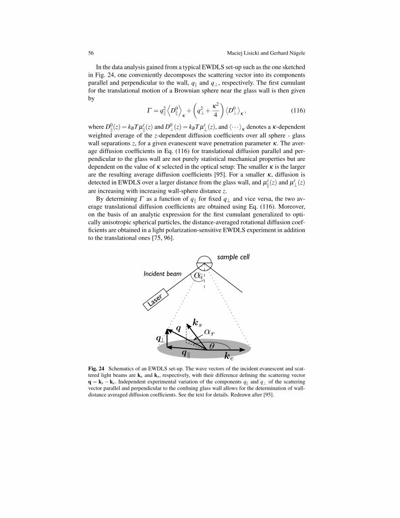
56 Maciej Lisicki and Gerhard Nagele
In the data analysis gained from a typical EWDLS set-up such as the one sketchedin Fig. 24, one conveniently decomposes the scattering vector into its componentsparallel and perpendicular to the wall, q‖ and q⊥, respectively. The first cumulantfor the translational motion of a Brownian sphere near the glass wall is then givenby
Γ = q2‖
⟨D0‖
⟩κ
+
(q2⊥+
κ2
4
)⟨D0⊥⟩
κ, (116)
where D0‖(z) = kBT µ t
‖(z) and D0⊥(z) = kBT µ t
⊥(z), and 〈· · · 〉κ
denotes a κ-dependentweighted average of the z-dependent diffusion coefficients over all sphere - glasswall separations z, for a given evanescent wave penetration parameter κ . The aver-age diffusion coefficients in Eq. (116) for translational diffusion parallel and per-pendicular to the glass wall are not purely statistical mechanical properties but aredependent on the value of κ selected in the optical setup: The smaller κ is the largerare the resulting average diffusion coefficients [95]. For a smaller κ , diffusion isdetected in EWDLS over a larger distance from the glass wall, and µ t
‖(z) and µ t⊥(z)
are increasing with increasing wall-sphere distance z.By determining Γ as a function of q‖ for fixed q⊥ and vice versa, the two av-
erage translational diffusion coefficients are obtained using Eq. (116). Moreover,on the basis of an analytic expression for the first cumulant generalized to opti-cally anisotropic spherical particles, the distance-averaged rotational diffusion coef-ficients are obtained in a light polarization-sensitive EWDLS experiment in additionto the translational ones [75, 96].
Laser
Incident beam
sample cell
Fig. 24 Schematics of an EWDLS set-up. The wave vectors of the incident evanescent and scat-tered light beams are ke and ks, respectively, with their difference defining the scattering vectorq = ks− ke. Independent experimental variation of the components q‖ and q⊥ of the scatteringvector parallel and perpendicular to the confining glass wall allows for the determination of wall-distance averaged diffusion coefficients. See the text for details. Redrawn after [95].
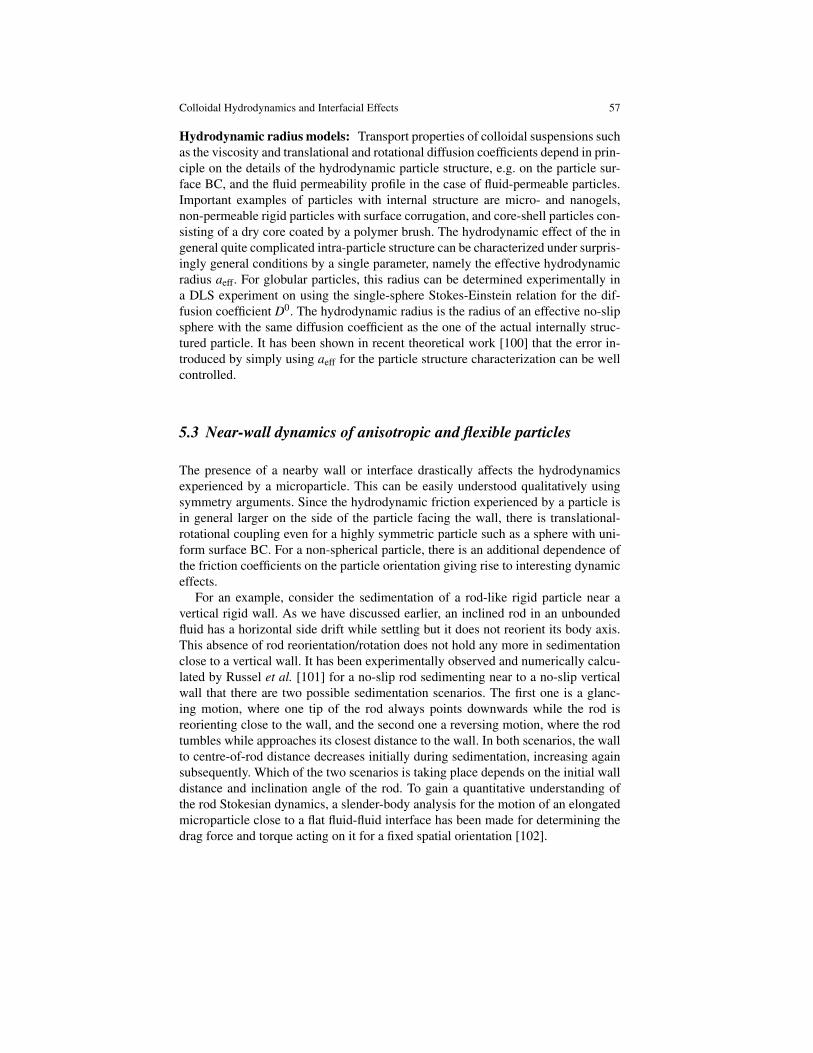
Colloidal Hydrodynamics and Interfacial Effects 57
Hydrodynamic radius models: Transport properties of colloidal suspensions suchas the viscosity and translational and rotational diffusion coefficients depend in prin-ciple on the details of the hydrodynamic particle structure, e.g. on the particle sur-face BC, and the fluid permeability profile in the case of fluid-permeable particles.Important examples of particles with internal structure are micro- and nanogels,non-permeable rigid particles with surface corrugation, and core-shell particles con-sisting of a dry core coated by a polymer brush. The hydrodynamic effect of the ingeneral quite complicated intra-particle structure can be characterized under surpris-ingly general conditions by a single parameter, namely the effective hydrodynamicradius aeff. For globular particles, this radius can be determined experimentally ina DLS experiment on using the single-sphere Stokes-Einstein relation for the dif-fusion coefficient D0. The hydrodynamic radius is the radius of an effective no-slipsphere with the same diffusion coefficient as the one of the actual internally struc-tured particle. It has been shown in recent theoretical work [100] that the error in-troduced by simply using aeff for the particle structure characterization can be wellcontrolled.
5.3 Near-wall dynamics of anisotropic and flexible particles
The presence of a nearby wall or interface drastically affects the hydrodynamicsexperienced by a microparticle. This can be easily understood qualitatively usingsymmetry arguments. Since the hydrodynamic friction experienced by a particle isin general larger on the side of the particle facing the wall, there is translational-rotational coupling even for a highly symmetric particle such as a sphere with uni-form surface BC. For a non-spherical particle, there is an additional dependence ofthe friction coefficients on the particle orientation giving rise to interesting dynamiceffects.
For an example, consider the sedimentation of a rod-like rigid particle near avertical rigid wall. As we have discussed earlier, an inclined rod in an unboundedfluid has a horizontal side drift while settling but it does not reorient its body axis.This absence of rod reorientation/rotation does not hold any more in sedimentationclose to a vertical wall. It has been experimentally observed and numerically calcu-lated by Russel et al. [101] for a no-slip rod sedimenting near to a no-slip verticalwall that there are two possible sedimentation scenarios. The first one is a glanc-ing motion, where one tip of the rod always points downwards while the rod isreorienting close to the wall, and the second one a reversing motion, where the rodtumbles while approaches its closest distance to the wall. In both scenarios, the wallto centre-of-rod distance decreases initially during sedimentation, increasing againsubsequently. Which of the two scenarios is taking place depends on the initial walldistance and inclination angle of the rod. To gain a quantitative understanding ofthe rod Stokesian dynamics, a slender-body analysis for the motion of an elongatedmicroparticle close to a flat fluid-fluid interface has been made for determining thedrag force and torque acting on it for a fixed spatial orientation [102].
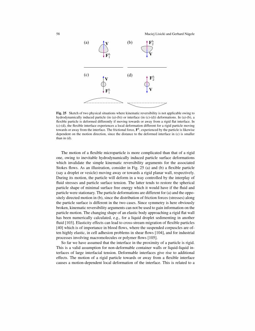
58 Maciej Lisicki and Gerhard Nagele
(a) (b)
(c) (d)
Fig. 25 Sketch of two physical situations where kinematic reversibility is not applicable owing tohydrodynamically induced particle (in (a)-(b)) or interface (in (c)-(d)) deformations. In (a)-(b), aflexible particle is deformed differently if moving towards or away from a rigid flat interface. In(c)-(d), the flexible interface experiences a local deformation different for a rigid particle movingtowards or away from the interface. The frictional force, Fh, experienced by the particle is likewisedependent on the motion direction, since the distance to the deformed interface in (c) is smallerthan in (d).
The motion of a flexible microparticle is more complicated than that of a rigidone, owing to inevitable hydrodynamically induced particle surface deformationswhich invalidate the simple kinematic reversibility arguments for the associatedStokes flows. As an illustration, consider in Fig. 25 (a) and (b) a flexible particle(say a droplet or vesicle) moving away or towards a rigid planar wall, respectively.During its motion, the particle will deform in a way controlled by the interplay offluid stresses and particle surface tension. The latter tends to restore the sphericalparticle shape of minimal surface free energy which it would have if the fluid andparticle were stationary. The particle deformations are different for (a) and the oppo-sitely directed motion in (b), since the distribution of friction forces (stresses) alongthe particle surface is different in the two cases. Since symmetry is here obviouslybroken, kinematic reversibility arguments can not be used to gain information on theparticle motion. The changing shape of an elastic body approaching a rigid flat wallhas been numerically calculated, e.g., for a liquid droplet sedimenting in anotherfluid [103]. Elasticity effects can lead to cross-stream migration of flexible particles[40] which is of importance in blood flows, where the suspended corpuscles are of-ten highly elastic, in cell adhesion problems in shear flows [104], and for industrialprocesses involving macromolecules or polymer flows [105].
So far we have assumed that the interface in the proximity of a particle is rigid.This is a valid assumption for non-deformable container walls or liquid-liquid in-terfaces of large interfacial tension. Deformable interfaces give rise to additionaleffects. The motion of a rigid particle towards or away from a flexible interfacecauses a motion-dependent local deformation of the interface. This is related to a
Colloidal Hydrodynamics and Interfacial Effects 59
special type of particle-interface interaction through the geometric coupling of lo-cal interface shape and flow [106]. A rigid particle moving away from the interfacesketched in Fig. 25(c) pulls the fluid along with it which in turn causes a local de-formation in the flexible interface extending in the direction of the particle motion.This results in an enlarged hydrodynamic friction force on the particle as comparedto the flat-surface situation, i.e. Fh
1 >Fhflat. The geometric coupling for the oppositely
oriented particle motion in figure part (d) leads to a frictional force on the particlesmaller than in the flat interface case so that Fh
2 < Fhflat. This is reminiscent of the lift
force acting on deformable particles in flow, and is of interest for biological systemflows under elastic confinement. Quite interestingly, the vicinity of a soft interfaceor object can be used by microorganisms in their propulsion even if performing re-ciprocal motions [107], since the micro-scallop theorem discussed in Sec. 6 doesnot apply near a flexible surface [108].
6 Self-propelling microswimmers
The locomotion and transport of autonomous (self-propelling) biological and arti-ficial microswimmers under low-Reynolds-number flow conditions has generateda lot of interest over the past years. See here [108, 109] for two very informativeoverview articles, and a classical book by Lighthill [110]. The motility of microor-ganisms such as bacteria, sperm cells, and algae affects many biological processesincluding reproduction and infection. Appropriate swimming strategies are essen-tial for microorganisms in their search for food or the avoidance of toxic environ-ments (chemotaxis), the reaction to light (phototaxis), and the orientation undergravity (gravitaxis). The theoretical design and fabrication of synthetic (robotic)microswimmers who can transport cargo or remove toxins bears the perspective ofhighly useful applications in medicine, biology and environmental science.
Autonomous swimmers are characterized by the absence of an external forcingagent driving their translational and rotational motion. For microswimmers underStokes-flow conditions, this means
Fh(t) = 0 , Th(t) = 0 , (117)
expressing that the total hydrodynamic drag force and torque exerted on the swim-mers are zero at any instant of time. The long-distance decay of the disturbance fluidvelocity field caused by the swimmer’s motion is thus of O(r−2) or faster.
There are a variety of autonomous propulsion mechanisms. For instance, a mi-croobject could swim by self-diffusiophoresis, by creating through a surface-activesite a small gradient, ∇φ , in the concentration φ of a dissolved species (solute). Thisself-created gradient, in turn, propels the microobject through the phoretic osmoticsolute flow in its interfacial region [48, 52], with the self-phoretic velocity, Vphor,of the object determined by Eq. (79). The potential flow outside the self-phoreticobject has thus the characteristic O(r−3) far-distance decay.
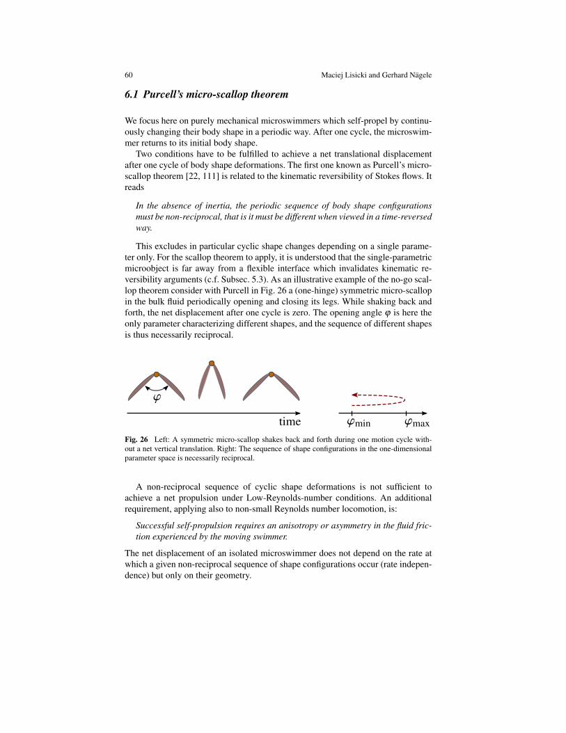
60 Maciej Lisicki and Gerhard Nagele
6.1 Purcell’s micro-scallop theorem
We focus here on purely mechanical microswimmers which self-propel by continu-ously changing their body shape in a periodic way. After one cycle, the microswim-mer returns to its initial body shape.
Two conditions have to be fulfilled to achieve a net translational displacementafter one cycle of body shape deformations. The first one known as Purcell’s micro-scallop theorem [22, 111] is related to the kinematic reversibility of Stokes flows. Itreads
In the absence of inertia, the periodic sequence of body shape configurationsmust be non-reciprocal, that is it must be different when viewed in a time-reversedway.
This excludes in particular cyclic shape changes depending on a single parame-ter only. For the scallop theorem to apply, it is understood that the single-parametricmicroobject is far away from a flexible interface which invalidates kinematic re-versibility arguments (c.f. Subsec. 5.3). As an illustrative example of the no-go scal-lop theorem consider with Purcell in Fig. 26 a (one-hinge) symmetric micro-scallopin the bulk fluid periodically opening and closing its legs. While shaking back andforth, the net displacement after one cycle is zero. The opening angle ϕ is here theonly parameter characterizing different shapes, and the sequence of different shapesis thus necessarily reciprocal.
Fig. 26 Left: A symmetric micro-scallop shakes back and forth during one motion cycle with-out a net vertical translation. Right: The sequence of shape configurations in the one-dimensionalparameter space is necessarily reciprocal.
A non-reciprocal sequence of cyclic shape deformations is not sufficient toachieve a net propulsion under Low-Reynolds-number conditions. An additionalrequirement, applying also to non-small Reynolds number locomotion, is:
Successful self-propulsion requires an anisotropy or asymmetry in the fluid fric-tion experienced by the moving swimmer.
The net displacement of an isolated microswimmer does not depend on the rate atwhich a given non-reciprocal sequence of shape configurations occur (rate indepen-dence) but only on their geometry.
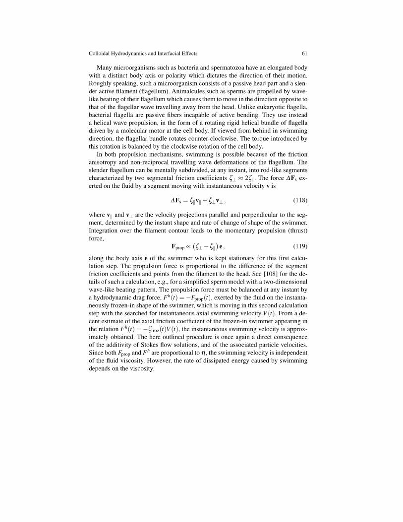
Colloidal Hydrodynamics and Interfacial Effects 61
Many microorganisms such as bacteria and spermatozoa have an elongated bodywith a distinct body axis or polarity which dictates the direction of their motion.Roughly speaking, such a microorganism consists of a passive head part and a slen-der active filament (flagellum). Animalcules such as sperms are propelled by wave-like beating of their flagellum which causes them to move in the direction opposite tothat of the flagellar wave travelling away from the head. Unlike eukaryotic flagella,bacterial flagella are passive fibers incapable of active bending. They use insteada helical wave propulsion, in the form of a rotating rigid helical bundle of flagelladriven by a molecular motor at the cell body. If viewed from behind in swimmingdirection, the flagellar bundle rotates counter-clockwise. The torque introduced bythis rotation is balanced by the clockwise rotation of the cell body.
In both propulsion mechanisms, swimming is possible because of the frictionanisotropy and non-reciprocal travelling wave deformations of the flagellum. Theslender flagellum can be mentally subdivided, at any instant, into rod-like segmentscharacterized by two segmental friction coefficients ζ⊥ ≈ 2ζ‖. The force ∆Fs ex-erted on the fluid by a segment moving with instantaneous velocity v is
∆Fs = ζ‖v‖+ζ⊥v⊥ , (118)
where v‖ and v⊥ are the velocity projections parallel and perpendicular to the seg-ment, determined by the instant shape and rate of change of shape of the swimmer.Integration over the filament contour leads to the momentary propulsion (thrust)force,
Fprop ∝(ζ⊥−ζ‖
)e , (119)
along the body axis e of the swimmer who is kept stationary for this first calcu-lation step. The propulsion force is proportional to the difference of the segmentfriction coefficients and points from the filament to the head. See [108] for the de-tails of such a calculation, e.g., for a simplified sperm model with a two-dimensionalwave-like beating pattern. The propulsion force must be balanced at any instant bya hydrodynamic drag force, Fh(t) =−Fprop(t), exerted by the fluid on the instanta-neously frozen-in shape of the swimmer, which is moving in this second calculationstep with the searched for instantaneous axial swimming velocity V (t). From a de-cent estimate of the axial friction coefficient of the frozen-in swimmer appearing inthe relation Fh(t) =−ζfroz(t)V (t), the instantaneous swimming velocity is approx-imately obtained. The here outlined procedure is once again a direct consequenceof the additivity of Stokes flow solutions, and of the associated particle velocities.Since both Fprop and Fh are proportional to η , the swimming velocity is independentof the fluid viscosity. However, the rate of dissipated energy caused by swimmingdepends on the viscosity.
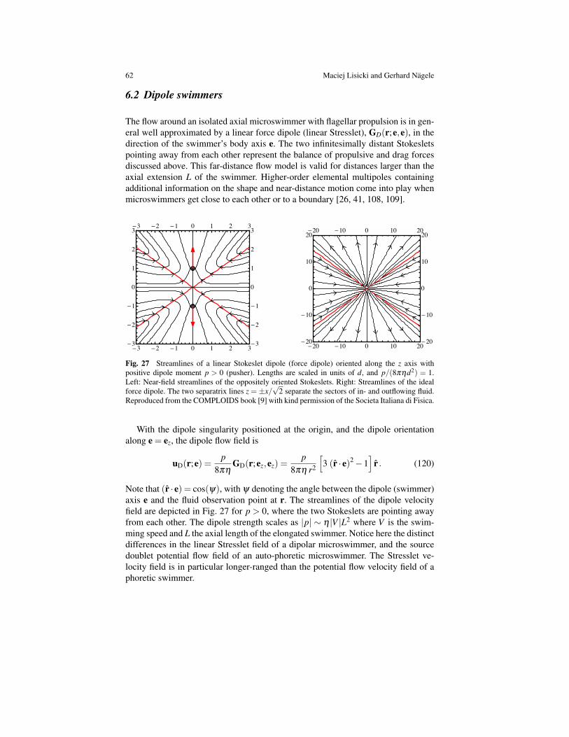
62 Maciej Lisicki and Gerhard Nagele
6.2 Dipole swimmers
The flow around an isolated axial microswimmer with flagellar propulsion is in gen-eral well approximated by a linear force dipole (linear Stresslet), GD(r;e,e), in thedirection of the swimmer’s body axis e. The two infinitesimally distant Stokesletspointing away from each other represent the balance of propulsive and drag forcesdiscussed above. This far-distance flow model is valid for distances larger than theaxial extension L of the swimmer. Higher-order elemental multipoles containingadditional information on the shape and near-distance motion come into play whenmicroswimmers get close to each other or to a boundary [26, 41, 108, 109].
-3 -2 -1 0 1 2 3-3
-2
-1
0
1
2
3-3 -2 -1 0 1 2 3
-3
-2
-1
0
1
2
3
-20 -10 0 10 20-20
-10
0
10
20-20 -10 0 10 20
-20
-10
0
10
20
Fig. 27 Streamlines of a linear Stokeslet dipole (force dipole) oriented along the z axis withpositive dipole moment p > 0 (pusher). Lengths are scaled in units of d, and p/(8πηd2) = 1.Left: Near-field streamlines of the oppositely oriented Stokeslets. Right: Streamlines of the idealforce dipole. The two separatrix lines z =±x/
√2 separate the sectors of in- and outflowing fluid.
Reproduced from the COMPLOIDS book [9] with kind permission of the Societa Italiana di Fisica.
With the dipole singularity positioned at the origin, and the dipole orientationalong e = ez, the dipole flow field is
uD(r;e) =p
8πηGD(r;ez,ez) =
p8πη r2
[3 (r · e)2−1
]r . (120)
Note that (r · e) = cos(ψ), with ψ denoting the angle between the dipole (swimmer)axis e and the fluid observation point at r. The streamlines of the dipole velocityfield are depicted in Fig. 27 for p > 0, where the two Stokeslets are pointing awayfrom each other. The dipole strength scales as |p| ∼ η |V |L2 where V is the swim-ming speed and L the axial length of the elongated swimmer. Notice here the distinctdifferences in the linear Stresslet field of a dipolar microswimmer, and the sourcedoublet potential flow field of an auto-phoretic microswimmer. The Stresslet ve-locity field is in particular longer-ranged than the potential flow velocity field of aphoretic swimmer.
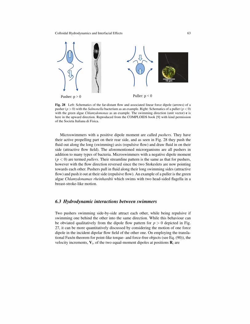
Colloidal Hydrodynamics and Interfacial Effects 63
Pusher: p > 0 Puller: p < 0
Fig. 28 Left: Schematics of the far-distant flow and associated linear force dipole (arrows) of apusher (p > 0) with the Salmonella bacterium as an example. Right: Schematics of a puller (p < 0)with the green algae Chlamydomonas as an example. The swimming direction (unit vector) e ishere in the upward direction. Reproduced from the COMPLOIDS book [9] with kind permissionof the Societa Italiana di Fisica.
Microswimmers with a positive dipole moment are called pushers. They havetheir active propelling part on their rear side, and as seen in Fig. 28 they push thefluid out along the long (swimming) axis (repulsive flow) and draw fluid in on theirside (attractive flow field). The aforementioned microrganisms are all pushers inaddition to many types of bacteria. Microswimmers with a negative dipole moment(p < 0) are termed pullers. Their streamline pattern is the same as that for pushers,however with the flow direction reversed since the two Stokeslets are now pointingtowards each other. Pushers pull in fluid along their long swimming sides (attractiveflow) and push it out at their side (repulsive flow). An example of a puller is the greenalgae Chlamydonamas rheinhardtii which swims with two head-sided flagella in abreast-stroke-like motion.
6.3 Hydrodynamic interactions between swimmers
Two pushers swimming side-by-side attract each other, while being repulsive ifswimming one behind the other into the same direction. While this behaviour canbe obviated qualitatively from the dipole flow pattern for p > 0 depicted in Fig.27, it can be more quantitatively discussed by considering the motion of one forcedipole in the incident dipolar flow field of the other one. On employing the transla-tional Faxen theorem for point-like torque- and force-free objects (see Eq. (90)), thevelocity increments, Vi, of the two equal-moment dipoles at positions Ri are
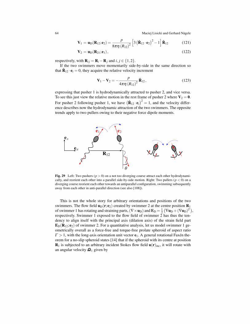
64 Maciej Lisicki and Gerhard Nagele
V1 = uD(R12;e2) =p
8πη (R12)2
[3(R12 · e2
)2−1]
R12 (121)
V2 = uD(R21;e1) , (122)
respectively, with Ri j = Ri−R j and i, j ∈ 1,2.If the two swimmers move momentarily side-by-side in the same direction so
that R12 · ei = 0, they acquire the relative velocity increment
V1−V2 =−p
4πη (R12)2 R12 , (123)
expressing that pusher 1 is hydrodynamically attracted to pusher 2, and vice versa.To see this just view the relative motion in the rest frame of pusher 2 where V2 = 0.For pusher 2 following pusher 1, we have
(R12 · ei
)2= 1, and the velocity differ-
ence describes now the hydrodynamic attraction of the two swimmers. The oppositetrends apply to two pullers owing to their negative force dipole moments.
Fig. 29 Left: Two pushers (p > 0) on a not too diverging course attract each other hydrodynami-cally, and reorient each other into a parallel side-by-side motion. Right: Two pullers (p < 0) on adiverging course reorient each other towards an antiparallel configuration, swimming subsequentlyaway from each other in anti-parallel direction (see also [108]).
This is not the whole story for arbitrary orientations and positions of the twoswimmers. The flow field uD(r;e2) created by swimmer 2 at the centre position R1of swimmer 1 has rotating and straining parts, (∇×uD) and ED = 1
2
(∇uD +(∇uD)
T),
respectively. Swimmer 1 exposed to the flow field of swimmer 2 has thus the ten-dency to align itself with the principal axis (dilation axis) of the strain field partED(R12;e2) of swimmer 2. For a quantitative analysis, let us model swimmer 1 ge-ometrically overall as a force-free and torque-free prolate spheroid of aspect ratioΓ > 1, with the long-axis orientation unit vector e1. A general rotational Faxen the-orem for a no-slip spheroid states [14] that if the spheroid with its centre at positionR1 is subjected to an arbitrary incident Stokes flow field u(r)inc, it will rotate withan angular velocity ΩΩΩ 1 given by
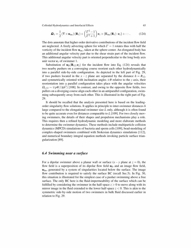
Colloidal Hydrodynamics and Interfacial Effects 65
ΩΩΩ 1 =12(∇×uinc)(R1)+
(Γ 2−1Γ 2 +1
)e1×
(Einc(R1) · e1
)+ · · · . (124)
The dots annotate that higher order derivative contributions of the incident flow fieldare neglected. A freely advecting sphere for which Γ = 1 rotates thus with half thevorticity of the incident flow uinc, taken at the sphere center. An elongated body hasan additional angular velocity part due to the shear strain part of the incident flow.This additional angular velocity part is oriented perpendicular to the long body axisunit vector e1 of swimmer 1.
Substitution of uD(R12;e2) for the incident flow into Eq. (124) reveals thattwo nearby pushers on a converging course reorient each other hydrodynamicallyinto a parallel side-by-side configuration. As depicted in the left part of Fig. 29,if two pushers located in the x− z plane are separated by the distance h = R12,and symmetrically oriented with inclination angles ±θ relative to the z axis, theirreorientation into a parallel configuration takes place with the angular velocitiesΩy,12 ∼ ∓pθ/(ηh3) [108]. In contrast, and owing to the opposite flow fields, twopullers on a diverging course align each other in an antiparallel configuration, swim-ming subsequently away from each other. This is illustrated in the right part of Fig.29.
It should be recalled that the analysis presented here is based on the leading-order singularity flow solutions. It applies in principle to inter-swimmer distances hlarge compared to the elongational swimmer size L only, although it is often foundto be quite accurate even for distances comparable to L [109]. For two closely mov-ing swimmers, the details of their shapes and propulsion mechanisms play a role.This requires then a refined hydrodynamic modeling and more elaborate methodsto determine the swimmer dynamics. These methods include multiparticle collisiondynamics (MPCD) simulations of bacteria and sperm cells [109], bead-modeling ofcomplex-shaped swimmers combined with Stokesian dynamics simulations [112],and numerical boundary integral equation methods invoking particle surface trian-gularization [89].
6.4 Swimming near a surface
For a dipolar swimmer above a planar wall or surface (x− y plane at z = 0), theflow field is a superposition of its dipolar flow field uD and an image flow field,uIm, generated by a system of singularities located below the surface. The imageflow contribution is required to satisfy the surface BC (recall Sec.5). In Fig. 30,this situation is illustrated for the simplest case of a pusher swimming above a freesurface. The only BC here is the fluid-impermeability of the surface which can befulfilled by considering the swimmer in the half-space z > 0 to move along with itsmirror image in the fluid extended to the lower half-space z < 0. This is akin to thesymmetric side-by-side motion of two swimmers in bulk fluid discussed earlier inrelation to Fig. 29.
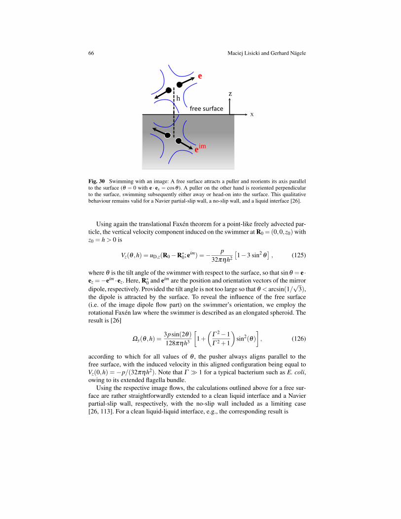
66 Maciej Lisicki and Gerhard Nagele
52
free surface h
Dipole swimmer near a surface
X
z
im imD 0 D 0( ; ) ( ; )= − + −u
( )r
u r R e u r R e
adv im imz 0 D
2
,z 0 0
2
hp
32
u ( ) u ( ; )
1 3cosπη
= −
= − − θ
R R R e
e
ime( )
3adv 2y 0
3p sin
128 h
2( ) 2 cosπη
θ Ω = − − θ R
xcosθ = ⋅e e
Interface always attracts pusher and orients it parallel to surface
Interface always repels puller, orienting it perpendicular to interface
Fig. 30 Swimming with an image: A free surface attracts a puller and reorients its axis parallelto the surface (θ = 0 with e · ex = cosθ ). A puller on the other hand is reoriented perpendicularto the surface, swimming subsequently either away or head-on into the surface. This qualitativebehaviour remains valid for a Navier partial-slip wall, a no-slip wall, and a liquid interface [26].
Using again the translational Faxen theorem for a point-like freely advected par-ticle, the vertical velocity component induced on the swimmer at R0 = (0,0,z0) withz0 = h > 0 is
Vz(θ ,h) = uD,z(R0−R∗0;eim) =− p32πηh2
[1−3 sin2
θ], (125)
where θ is the tilt angle of the swimmer with respect to the surface, so that sinθ = e ·ez =−eim ·ez. Here, R∗0 and eim are the position and orientation vectors of the mirrordipole, respectively. Provided the tilt angle is not too large so that θ < arcsin(1/
√3),
the dipole is attracted by the surface. To reveal the influence of the free surface(i.e. of the image dipole flow part) on the swimmer’s orientation, we employ therotational Faxen law where the swimmer is described as an elongated spheroid. Theresult is [26]
Ωy(θ ,h) =3psin(2θ)
128πηh3
[1+(
Γ 2−1Γ 2 +1
)sin2(θ)
], (126)
according to which for all values of θ , the pusher always aligns parallel to thefree surface, with the induced velocity in this aligned configuration being equal toVz(0,h) = −p/(32πηh2). Note that Γ 1 for a typical bacterium such as E. coli,owing to its extended flagella bundle.
Using the respective image flows, the calculations outlined above for a free sur-face are rather straightforwardly extended to a clean liquid interface and a Navierpartial-slip wall, respectively, with the no-slip wall included as a limiting case[26, 113]. For a clean liquid-liquid interface, e.g., the corresponding result is
Colloidal Hydrodynamics and Interfacial Effects 67
Ωy(θ ,h) =3psin(2θ)
128πη1h3
[1+
12
(Γ 2−1Γ 2 +1
)(λ +(2+λ )sin2(θ)
1+λ
)](127)
Vz(0,h) = −p(2+3λ )
32πη1 (1+λ )h2 , (128)
with the free and no-slip surface results recovered as the limiting cases for λ =η2/η1 = 0 and λ → ∞, respectively. A pusher is always attracted by and aligned toa nearby liquid interface, for any value of the viscosity ratio. The pusher is likewiseattracted and aligned parallel by a partial-slip wall, for any value of the Navier sliplength [26].
The attraction by and the accumulation of biological microswimmers near sur-faces is indeed observed in many biological experiments. According to the aboveanalysis, pullers are oriented hydrodynamically in the direction perpendicular to thesurface (θ =±π/2), swimming either head-on away or right into the surface.
The simple modeling of pushers as linear force dipoles gives the prediction thatthey should move in straight trajectories along a surface, owing to the rotationalsymmetry of the aligned dipole with respect to the surface normal. However, it isknown experimentally that bacteria such as E. coli do swim in clockwise (CW)traversed circles along a glass surface [114], as viewed from inside the fluid, whereasnear a clean free surface the spherical trajectories are traversed counter-clockwise(CCW). The CW circular motion near the glass plate can be changed to a CCWmotion if a sufficient amount of free polymers is added to the fluid. Likewise, theCW circular motion at a clean free surface can change to a CCW motion uponthe addition of detergents accumulating at the surface. The circular motion of abacterium is interrupted when a tumbling event occurs.
This surface-specificity of the trajectories can be attributed to the chiral bacterialpropulsion mechanism not resolved in the simple force dipole model. It becomesessential when the swimmer gets close to a surface. To understand qualitatively theCCW circular motion of a pusher near a free surface, recall that this is equivalent toa pusher swimming in the flow field of its image. The image moves with the samespeed as the actual pusher, but the helical flagellar bundle (cell body) of the imagerotates opposite to that of the pusher. Recall that the bundle of a bacterium rotatescounterclockwise if viewed from behind, and suppose that the bacterium is orientedmomentarily along the y-axis. The counter-rotating flagellar helices (cell bodies) ofthe swimmer and its image create then a disturbance flow directed in the positive(negative) x-direction. Since the swimmer is freely advecting in this flow, it willperform a CCW circular motion [115]. Qualitative arguments similar to the presentones can be given to explain the CW circular motion of a bacterium at a no-slipsurface where an advection flow oppositely directed to that near a free surface iscreated [108].
As Lopez and Lauga have recently shown [26], the surface-specific circular mo-tion of a bacterium is quantitatively explainable on the singularity method level byadding a so-called rotlet dipole singularity solution, uRD(r)∼ O(r−3), to the linearforce dipole solution of O(r−2). The rotlet dipole part accounts on the long-distancelevel for the counter-rotating flagellum and cell body parts of the torque-free pusher.
68 Maciej Lisicki and Gerhard Nagele
Using this flow singularity model in conjunction with surface-specific image sys-tems, interesting quantitative predictions regarding critical parameter values for theCW to CCW motion transition for partial-slip walls and surfactant-covered inter-faces have been made [26].
7 Concluding Remarks
The present notes give an introduction into the world of low-Reynolds-number flowsand associated passive and active (i.e. self-propelling) microparticle motions, withthe focus on surface and interfacial effects. As the topics treated in the notes shouldhave amply illustrated, studying low-Reynolds-number phenomena is important,and often leads to surprising findings. Our aim has been to provide the reader withbasic background knowledge which facilitates further reading of more advancedresearch texts on processes involving microparticles and animalcules suspended inviscous fluids. We have presented the governing equations of Stokes flows and theiressential properties in a rather descriptive way, avoiding detailed calculations whichcan be found in more specialized textbooks and overview papers. While the ma-terial is presented in a rather systematic way, many important phenomena such asMarangoni surface flows [23], hydrodynamic screening near boundaries [116], wall-induced apparent like-charge attraction of colloidal macroions [117, 118], and hy-drodynamically induced surface accumulation of microparticles [119, 55, 120] havebeen only shortly addressed, with an occasional reference to related literature, oreven not mentioned at all. The present notes can serve as a good preparation for animproved understanding of research papers on these additional phenomena.
Acknowledgments: These notes include and complement material which was pre-sented in August 2014 at the SOMATAI summer school in Berlin, and in March2014 at the SOMATAI workshop in Julich. It is our pleasure to thank the organizerof these events, Peter Lang, for having invited us to present a lecture on the colloidalhydrodynamics of microparticles and associated interfacial effects. We thank MariaEkiel-Jezewska (Polish Academy of Sciences, Warsaw) for having provided us withthe streamlines figures of a point force near a planar interface, and Jonas Riest andRafael Roa (ICS-3, FZ Julich) and Roland Winkler (IAS-2, FZ Julich) for helpfuldiscussions. Moreover, we are grateful to Ulrike Nagele (FZ Julich, ICS-3) for herhelp with travel and accommodation.
References
1. J. K. G. Dhont, An Introduction to Dynamics of Colloids, Elsevier, 1996.2. P. Szymczak and M. Cieplak, J. Physics. Condens. Matter. 23, 033102 (2011).3. R. G. Larson and J. J. Magda, Macromolecules 22, 3004 (1989).4. H. Tanaka, J. Phys. Condens. Matter 13, 4637 (2001).5. P. Wojtaszczyk and J. B. Avalos, Phys. Rev. Lett. 80, 754 (1998).
Colloidal Hydrodynamics and Interfacial Effects 69
6. C. Korn and U. S. Schwarz, Phys. Rev. Lett. 97, 138103 (2006).7. O. B. Usta, J. E. Butler, and A. J. C. Ladd, Phys. Fluids 18, 031703 (2006).8. E. Guazzelli and J. F. Morris, A Physical Introduction to Suspension Dynamics, Cambridge
Univ. Press, 2012.9. G. Nagele, Colloidal Hydrodynamics, in Physics of Complex Colloids, edited by
C. Bechinger, F. Sciortino, and P. Ziherl, volume 184, Proceedings of the International Schoolof Physics ”Enrico Fermi”, page 451, IOS Press, Amsterdam; SIF, Bologna, 2012.
10. G. Nagele, Dynamics of Charged-Particles Dispersions, in Proceedings of the 5th WarsawSchool of Statistical Physics, page 83, Warsaw Univ. Press, 2014.
11. E. J. Hinch, Hydrodynamics at Low Reynolds Numbers: A Brief and Elementary Introduc-tion, in Disorder and Mixing, edited by E. Guyon, J.-P. Nadal, and Y. Pomeau, volume 2,pages 43–55, Springer Netherlands, 1988.
12. P. N. Pusey, Colloidal Suspensions, in Liquids, Freezing and Glass Transition, edited by J. P.Hansen, D. Levesque, and J. Zinn-Justin, page 763, Elsevier, Amsterdam, 1991.
13. R. B. Jones and P. N. Pusey, Annu. Rev. Phys. Chem. 42, 137 (1991).14. S. Kim and S. J. Karrila, Microhydrodynamics: Principles and Selected Applications,
Butterworth- Heinemann, Boston, 1991.15. J. Happel and H. Brenner, Low Reynolds Numbers Hydrodynamics, Kluwer, Dordrecht,
1991.16. Z. Zapryanov and S. Tabakova, Dynamics of Bubbles, Drops and Rigid Particles, Fluid
Mechanics and Its Applications, Springer Netherlands, 2011.17. G. K. Batchelor, An Introduction to Fluid Dynamics, Cambridge Mathematical Library,
Cambridge Univ. Press, 2000.18. L. D. Landau and E. M. Lifshitz, Fluid Mechanics, Course of Theoretical Physics, Pergamon
Press, 1987.19. E. Guyon, J. P. Hulin, and L. Petit, Physical Hydrodynamics, Oxford Univ. Press, 2001.20. G. I. Taylor, Low Reynolds Number Flows, National Committe For Fluid Mechanics Films,
website: http://web.mit.edu/hml/ncfmf.html, 1966.21. W. B. Russel, D. A. Saville, and W. R. Schowalter, Colloidal Dispersions, Cambridge
Monographs on Mechanics, Cambridge University Press, 1989.22. E. Lauga, M. P. Brenner, and H. A. Stone, The No-Slip Boundary Condition, in Springer
Handbook of Experimental Fluid Mechanics, edited by C. Tropea, A. Yarin, and J. F. Foss,Springer, 2007.
23. L. G. Leal, Laminar Flow and Convective Transport Processes, Butterworth-Heinemann,1992.
24. N. Lecoq, R. Anthore, B. Cichocki, P. Szymczak, and F. Feuillebois, J. Fluid Mech. 513, 247(2004).
25. R. Tuinier and T. Taniguchi, J. Phys. Condens. Matter 17, L9 (2005).26. D. Lopez and E. Lauga, Phys. Fluids 26, 071902 (2014).27. K. H. Lan, N. Ostrowsky, and D. Sornette, Phys. Rev. Lett. 57, 17 (1986).28. B. Cichocki, M. L. Ekiel-Jezewska, and E. Wajnryb, J. Chem. Phys. 136, 071102 (2012).29. J. F. Brady and G. Bossis, Annu. Rev. Fluid Mech. 20, 111 (1988).30. I. M. Janosi, T. Tel, D. E. Wolf, and J. A. C. Gallas, Phys. Rev. E 56, 2858 (1997).31. M. L. Ekiel-Jezewska and E. Wajnryb, Phys. Rev. E 83, 067301 (2011).32. D. L. Ermak and J. A. McCammon, J. Chem. Phys. 69, 1352 (1978).33. G. Nagele, Brownian Dynamics simulations, in Computational Condensed Matter Physics,
volume 32, Forschungszentrum Julich Publishing, 37th IFF Spring School edition, 2006.34. A. T. Chwang and T. Wu, J. Fluid Mech. 67, 787 (1975).35. C. Pozrikidis, Boundary Integral and Singularity Methods for Linearized Viscous Flow,
Cambridge Univ. Press, 1992.36. J. D. Jackson, Classical Electrodynamics, John Wiley & Sons, 3rd edition, 1998.37. B. Cichocki, B. U. Felderhof, and K. Hinsen, J. Chem. Phys. 100, 3780 (1994).38. M. L. Ekiel-Jezewska and E. Wajnryb, Precise Multipole Method for Calculating Hydrody-
namic Interactions Between Spherical Particles in the Stokes Flow, in Theoretical Methodsfor Micro Scale Viscous Flows, edited by F. Feuillebois and A. Sellier, pages 127–172, 2009.
70 Maciej Lisicki and Gerhard Nagele
39. M. Lisicki, arXiv:1312.6231 [physics.flu-dyn] (2013).40. L. G. Leal, Annu. Rev. Fluid Mech. 12, 435 (1980).41. S. E. Spagnolie and E. Lauga, J. Fluid Mech. 700, 105 (2012).42. H. Luo and C. Pozrikidis, J. Eng. Math. 62, 1 (2007).43. G. K. Batchelor, Journal of Fluid Mechanics 44, 419 (1970).44. M. M. Tirado, C. L. Martinez, and J. G. de la Torre, J. Chem. Phys. 81, 2047 (1984).45. R. G. Cox, J. Fluid Mech. 44, 791 (1970).46. J. B. Keller and S. I. Rubinow, J. Fluid Mech. 75, 705 (1976).47. G. G. Stokes, Trans. Cambridge Philos. Soc. 9, 8 (1851).48. J. L. Anderson, Annu. Rev. Fluid Mech. 21, 61 (1989).49. J. H. Masliyah and S. Bhattacharjee, Electrokinetic and Colloid Transport Phenomena, John
Wiley & Sons, 2006.50. H. J. Keh and J. L. Anderson, J. Fluid Mech. 153, 417 (1985).51. A. S. Khair and T. M. Squires, Phys. Fluids 21, 042001 (2009).52. R. Golestanian, T. B. Liverpool, and A. Ajdari, New J. Phys. 9, 126 (2007).53. H. A. Stone and A. D. Samuel, Phys. Rev. Lett. 77, 4102 (1996).54. C. Contreras-Aburto and G. Nagele, J. Chem. Phys. 139, 134110 (2013).55. F. Weinert and D. Braun, Phys. Rev. Lett. 101, 168301 (2008).56. J. Rotne and S. Prager, J. Chem. Phys. 50, 4831 (1969).57. H. Yamakawa, J. Chem. Phys. 53, 436 (1970).58. E. Wajnryb, K. A. Mizerski, P. J. Zuk, and P. Szymczak, J. Fluid Mech. 731, R3 (2013).59. R. Courant and D. Hilbert, Methods of Mathematical Physics II, Interscience, New York,
1962.60. F. M. Weinert and D. Braun, Phys. Rev. Lett. 101, 168301 (2008).61. P. J. Zuk, E. Wajnryb, K. A. Mizerski, and P. Szymczak, J. Fluid Mech. 741, R5 (2014).62. B. Carrasco and J. Garcia de la Torre, Biophys J. 76, 3044 (1999).63. B. Cichocki, R. B. Jones, R. Kutteh, and E. Wajnryb, J. Chem. Phys. 112, 2548 (2000).64. S. Bhattacharya, J. Bawzdziewicz, and E. Wajnryb, Physica A 356, 294 (2005).65. M. Kedzierski and E. Wajnryb, J. Chem. Phys. 133, 154105 (2010).66. D. J. Acheson, Elementary Fluid Dynamics, Oxford Univ. Press, 1990.67. D. J. Jeffrey and Y. Onishi, J. Fluid Mech. 139, 261 (1984).68. R. Tadmor, J. Phys. Condens. Matter 13, L195 (2001).69. M. L. Ekiel-Jezewska and R. Boniecki, Stokes Flow Generated by a Point Force in Various
Geometries II. Velocity Field, Technical report, IFTR, Polish Acad. Sci., 2010.70. B. Cichocki, M. L. Ekiel-Jezewska, G. Nagele, and E. Wajnryb, J. Chem. Phys. 121, 2305
(2004).71. J. Blake, Proc. Camb. Phil. Soc. 70, 303 (1971).72. K. Aderogba and J. R. Blake, Bull. Aust. Math. Soc. 18, 345 (1978).73. J. Blake and A. Chwang, J. Eng. Math. 8, 23 (1974).74. E. Lauga and T. M. Squires, Phys. Fluids 17, 103102 (2005).75. M. Lisicki, B. Cichocki, S. A. Rogers, J. K. G. Dhont, and P. R. Lang, Soft Matter 10, 4312
(2014).76. B. Cichocki and R. B. Jones, Physica A 258, 273 (1998).77. H. A. Lorentz, Abhandlung uber Theoretische Physik, B. G. Teubner, Leipzig und Berlin,
1907.78. H. Faxen, Ark. Mat. Astron. Fys. 17, 1 (1923).79. H. Brenner, Chem. Eng. Sci. 16, 242 (1961).80. A. J. Goldman, R. G. Cox, and H. Brenner, Chem. Eng. Sci. 22, 637 (1967).81. A. J. Goldman, R. G. Cox, and H. Brenner, Chem. Eng. Sci. 22, 653 (1967).82. W. Dean and M. O’Neill, Mathematika 10, 13 (1963).83. W. Dean and M. O’Neill, Mathematika 11, 67 (1964).84. R. B. Jones, J. Chem. Phys. 123, 164705 (2005).85. B. Lin, J. Yu, and S. Rice, Phys. Rev. E 62, 3909 (2000).86. R. Sadr, C. Hohenegger, H. Li, P. J. Mucha, and M. Yoda, J. Fluid Mech. 577, 443 (2007).87. P. Huang and K. Breuer, Phys. Rev. E 76, 046307 (2007).
Colloidal Hydrodynamics and Interfacial Effects 71
88. L. Lobry and N. Ostrowsky, Phys. Rev. B 53, 12050 (1996).89. K. Ishii, T. Iwai, and H. Xia, Opt. Express 18, 7390 (2010).90. M. A. Plum, W. Steffen, G. Fytas, W. Knoll, and B. Menges, Opt. Express 17, 10364 (2009).91. M. A. Plum, J. Ricka, H.-J. Butt, and W. Steffen, New J. Phys. 12, 103022 (2010).92. P. Holmqvist, J. K. G. Dhont, and P. R. Lang, Phys. Rev. E 74, 021402 (2006).93. P. Holmqvist, J. K. G. Dhont, and P. R. Lang, J. Chem. Phys. 126, 044707 (2007).94. M. Hosoda, K. Sakai, and K. Takagi, Phys. Rev. E 58, 6275 (1998).95. M. Lisicki, B. Cichocki, J. K. G. Dhont, and P. R. Lang, J. Chem. Phys. 136, 204704 (2012).96. S. A. Rogers, M. Lisicki, B. Cichocki, J. K. G. Dhont, and P. R. Lang, Phys. Rev. Lett. 109,
098305 (2012).97. B. J. Berne and R. Pecora, Dynamic Light Scattering: With Applications to Chemistry, Biol-
ogy, and Physics, Dover Books on Physics Series, Dover Publications, 2000.98. R. Sigel, Curr. Opin. Colloid Interface Sci. 14, 426 (2009).99. G. Nagele, Phys. Rep. 272, 215 (1996).
100. B. Cichocki, M. L. Ekiel-Jezewska, and E. Wajnryb, J. Chem. Phys. 140, 164902 (2014).101. W. B. Russel, E. J. Hinch, L. G. Leal, and G. Tieffenbruck, J. Fluid Mech 83, 273 (1977).102. S.-M. Yang and L. G. Leal, J. Fluid Mech. 136, 393 (1983).103. E. P. Ascoli, D. S. Dandy, and L. G. Leal, J. Fluid Mech. 213, 287 (1990).104. I. Cantat and C. Misbah, Phys. Rev. Lett. 83, 880 (1999).105. U. S. Agarwal, A. Dutta, and R. A. Mashelkar, Chem. Eng. Sci. 49, 1693 (1994).106. C. Berdan and L. G. Leal, J. Colloid Interface Sci. 87, 62 (1982).107. R. Trouilloud, T. Yu, A. Hosoi, and E. Lauga, Phys. Rev. Lett. 101, 048102 (2008).108. E. Lauga and T. R. Powers, Rep. Prog. Phys. 72, 096601 (2009).109. J. Elgeti, R. G. Winkler, and G. Gompper, Rep. Prog. Phys. , accepted (2014).110. J. Lighthill, Mathematical Biofluiddynamics, SIAM, Philadelphia, 1975.111. E. M. Purcell, Am. J. Phys. 45, 3 (1977).112. J. W. Swan, J. F. Brady, and R. S. Moore, Phys. Fluids 23, 071901 (2011).113. A. P. Berke, L. Turner, H. C. Berg, and E. Lauga, Phys. Rev. Lett. 101, 038102 (2008).114. E. Lauga, W. R. DiLuzio, G. M. Whitesides, and H. A. Stone, Biophys. J. 90, 400 (2006).115. R. Di Leonardo, D. Dell’Arciprete, L. Angelani, and V. Iebba, Phys. Rev. Lett. , 038101
(2011).116. P. P. Lele, J. W. Swan, J. F. Brady, N. J. Wagner, and E. M. Furst, Soft Matter 7, 6844 (2011).117. T. Squires and M. Brenner, Phys. Rev. Lett. 85, 4976 (2000).118. T. M. Squires, J. Fluid Mech. 443, 403 (2001).119. R. Di Leonardo, F. Ianni, and G. Ruocco, Langmuir 25, 4247 (2009).120. J. Morthomas and A. Wurger, Phys. Rev. E 81, 051405 (2010).