collision prediction for a low power wide area network

Creative Commons Attribution-NonCommercial (CC BY-NC).This is an Open Access article distributed under the terms of Creative Commons Attribution Non-Commercial License (http://creativecommons.org/licenses/by-nc/3.0)

which permits unrestricted non-commercial use, distribution, and reproduction in any medium, provided that the original work is properly cited.

JOURNAL OF COMMUNICATIONS AND NETWORKS, VOL. 22, NO. 3, JUNE 2020 205

Collision Prediction for a Low Power Wide AreaNetwork using Deep Learning Methods

Shengmin Cui and Inwhee Joe

Abstract: A low power wide area network (LPWAN) is becominga popular technology since more and more industrial Internet ofthings (IoT) applications rely on it. It is able to provide long dis-tance wireless communication with great power saving. Given thefact that an LPWAN covers a wide area where all end nodes com-municate directly to a few gateways, a large number of devices haveto share the gateway. In this situation, chances are many collisionscould occur, leading to waste of limited wireless resources. How-ever, many factors affecting the number of collisions that cannotbe solved by traditional time series analysis algorithms. Therefore,deep learning methods can be applied here to predict collisions byanalyzing these factors in an LPWAN system. In this paper, wepropose long short-term memory extended Kalman filter (LSTM-EKF) model for collision prediction in the LPWAN in terms of thetemporal correlation which can improve the LSTM performance.The efficacies of our models are demonstrated on the data set sim-ulated by LoRaSim.

Index Terms: Deep Learning, extended Kalman filter, Internet ofthings, LoRa, LSTM.

I. INTRODUCTION

THE Internet of things (IoT) technology is changing ourlives since it has been incorporated in various fields. Exam-

ples of these areas include industrial automation, medical, smarthome, health management, transportation, and emergency re-sponse to man-made and natural disasters when it is difficult forhumans to make decisions [1]–[4]. IoT and machine-to-machine(M2M) industry will increase significantly over the next decadebased on multiple independent studies. Recent development ofsensors and new communication technologies support the pre-dicted trends. Low power wide area network (LPWAN) rep-resents a novel type of wireless communication that appearsto complement cellular networks and short-range wireless net-works to meet the diverse needs of IoT applications [5]. LP-WAN technology offers wide-area connectivity for low-powerand low-data-rate devices that traditional wireless technologiescannot. Traditional non-cellular wireless technologies such asZigBee, Bluetooth, Z-wave, and Wi-Fi are not suitable for con-necting to large geographical areas since they can only cover afew hundred meters. Therefore, these technologies cannot meet

Manuscript received October 22, 2019; revised May 29, 2020; approved forpublication by Yansha Deng, Guest Editor, May 31, 2020.

This work was supported by the National Research Foundation of Ko-rea (NRF) grant funded by the Korea government (MSIT) (No.NRF-2019R1A2C1009894)

S. Cui and I. Joe are with the Department of Computer Science, HanyangUniversity, email: {shengmincui, iwjoe}@hanyang.ac.kr.

I. Joe is the corresponding author.Digital Object Identifier: 10.1109/JCN.2020.000017

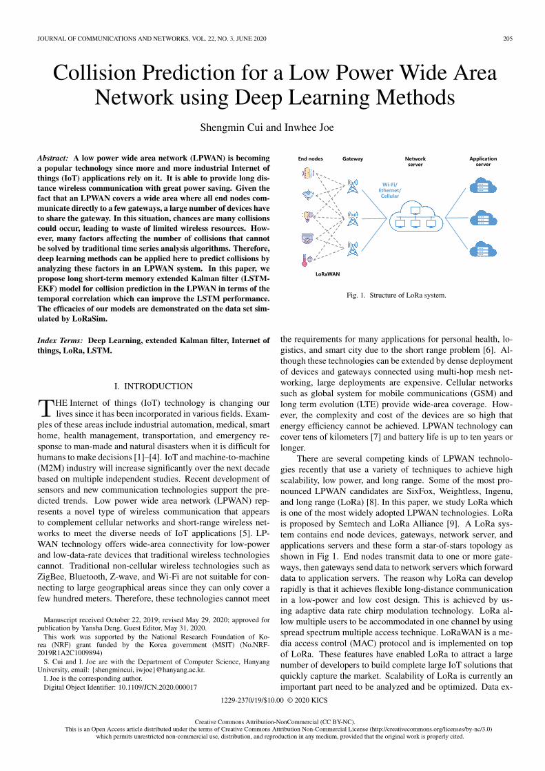
End nodes Gateway Network server

Application server

LoRaWAN

Wi-Fi/Ethernet/Cellular

Fig. 1. Structure of LoRa system.

the requirements for many applications for personal health, lo-gistics, and smart city due to the short range problem [6]. Al-though these technologies can be extended by dense deploymentof devices and gateways connected using multi-hop mesh net-working, large deployments are expensive. Cellular networkssuch as global system for mobile communications (GSM) andlong term evolution (LTE) provide wide-area coverage. How-ever, the complexity and cost of the devices are so high thatenergy efficiency cannot be achieved. LPWAN technology cancover tens of kilometers [7] and battery life is up to ten years orlonger.

There are several competing kinds of LPWAN technolo-gies recently that use a variety of techniques to achieve highscalability, low power, and long range. Some of the most pro-nounced LPWAN candidates are SixFox, Weightless, Ingenu,and long range (LoRa) [8]. In this paper, we study LoRa whichis one of the most widely adopted LPWAN technologies. LoRais proposed by Semtech and LoRa Alliance [9]. A LoRa sys-tem contains end node devices, gateways, network server, andapplications servers and these form a star-of-stars topology asshown in Fig 1. End nodes transmit data to one or more gate-ways, then gateways send data to network servers which forwarddata to application servers. The reason why LoRa can developrapidly is that it achieves flexible long-distance communicationin a low-power and low cost design. This is achieved by us-ing adaptive data rate chirp modulation technology. LoRa al-low multiple users to be accommodated in one channel by usingspread spectrum multiple access technique. LoRaWAN is a me-dia access control (MAC) protocol and is implemented on topof LoRa. These features have enabled LoRa to attract a largenumber of developers to build complete large IoT solutions thatquickly capture the market. Scalability of LoRa is currently animportant part need to be analyzed and be optimized. Data ex-

1229-2370/19/$10.00 © 2020 KICS

206 JOURNAL OF COMMUNICATIONS AND NETWORKS, VOL. 22, NO. 3, JUNE 2020

Fig. 2. Structure of SSM.

traction rate (DER) and network energy consumption (NEC) canbe used to evaluate the scalability of a LoRa system. Collisionsin the LoRa system have a great impact on DER and NEC [10]since LoRaWAN MAC protocol is essentially an ALOHA vari-ant with no collision avoidance provisions. Therefore, collisionprediction can help us to improve and analyze the parametersettings of LoRa and lay the foundation for intelligent resourceallocation.

Time series prediction has become one of popular researchtopics in recent years. Traditional time series prediction meth-ods predict future trend based on previously sampled values.Autoregressive moving average (ARMA) [11] algorithm is acombination of the autoregressive (AR) and moving average(MA) that predict the next values by constructing a linear func-tion of values observed and residual errors of prior time steps.Autoregressive integrated moving average (ARIMA) [11] is anextension of ARMA which makes prediction using linear func-tion of differenced observations and residual errors of priorsteps. State space model (SSM) is a ubiquitous tool for mod-eling time series data [12], [13] that only deals with one stepdependency. This is because an SSM is based on two assump-tions as shown in Fig 2: The output yt of SSM at time step tdepends on hidden state ht and external input ut with transferfunction g; the hidden state ht only depends on previous onestate ht−1 with transfer function f . However, these methodsonly make predictions based on observations and do not takeinto account internal influence factors. In this work, we shouldconsider not only the observations of the number of collisions,but also the factors affecting collisions should be considered inorder to improve the accuracy of the prediction. Therefore, weconsider machine learning (ML) and deep learning (DL) meth-ods which can learn the dynamic relationship between factorsand observations effectively.

ML technologies have made breakthroughs in various appli-cation fields, such as computer vision [14], [15], speech recog-nition [16], [17], and medicals [18], [19]. Algorithms and mod-els of ML can learn to make decisions directly from data with-out having to follow predefined rules. Existing ML algorithmsare generally divided into three categories: Supervised learn-ing (SL) that learns classification or regression tasks from la-beled data; unsupervised learning (USL) that focuses on clas-sifying sample data into different groups with unlabeled data;and reinforcement learning (RL) [20] that agents interact withthe environment and find the best actions to maximize reward.

Networking applications have also widely used machine learn-ing algorithms, such as traffic prediction, traffic classification,resource management, and network adaption [21], [22]. More-over, DL technologies also have made amazing achievements inmany fields. For instance, convolutional neural network (CNN)is typically employed for image recognition while recurrent neu-ral network (RNN) is frequently utilized for processing sequen-tial data [23]. An RNN model with its non-linear function canlearn more complicated pattern and has flexibility in modelingand can produce an output at each time step or read an entire se-quence and then produce a single output. Long short-term mem-ory (LSTM) [24] and gated recurrent unit (GRU) [25] are spe-cial RNN that solve the long term dependency by adding severalgates in the cell. These methods can model relationship betweeninfluence factors and number of collisions with non-linear func-tions. Among these methods LSTM achieves best performancein several time series data sets [26]–[28]. For the collision pre-diction issue in this paper, we combine the LSTM and SSM forprediction task that can improve the performance of LSTM. Ourmodel takes previous information of traffics in the LoRa sys-tem and make prediction of number of collisions in the future.The prediction results with different parameter settings are ex-amined to find the optimal settings and structure for collisionsprediction.

The organization of this paper is as follows. Related workfor LoRa scalability and collision problem are described in sec-tion II. Section III briefly explains collisions in LoRa system.Then our proposed models based on LSTM for collision predic-tion is presented in section IV. Next, comparisons of conven-tional models and proposal models are provided in section V.We then finalize our paper with conclusions in section VI.

II. RELATED WORK

There have been several works that focused on scalability andcollision of LoRa system. In [29], the authors studied how thenumber of end nodes and the throughput requirements affect thescalability of the LoRa system. They built a simulator for evalu-ating the scalability of a single gateway and their results shownthat when the number of end nodes increases to 1000, the pack-ets losses rate will be up to 32%. In [30], the authors proposeda model and present the effect of transmission using the samespreading factor (SF) and different SF on scalability of LoRasystem. They derived several signal-to-interference ratio (SIR)distributions in different conditions. The authors of [8] built amodel with a stochastic geometry framework for evaluating theLoRa system. Their results shown that the coverage probabil-ity decreases exponentially with the increase of number of endnodes when transmit using the same SF. The authors of [31] pro-posed single gateway and multiple gateway simulators for evalu-ating the scalability of the LoRa system with different parametercombinations.

On the other hand, there have been several works that com-mitted to improve the performance of the LoRa system. In [32],the authors modelled LoRa system with a new topology that lo-cations of end nodes follow a Poisson cluster process (PCP).Their work shown that the spectral efficiency and energy ef-ficiency can be obtained through adjusting the density of end

CUI et al.: COLLISION PREDICTION FOR A LOW POWER WIDE AREA ... 207

nodes around each gateways. In [33], a novel resource allocationmethod that using multi-layer virtual cell-based spatial time di-vision multiple access (STDMA) was proposed to improve per-formance of LoRa system. Their method that calculate schedulewith information of end nodes and fit the cell radius to fit thecommunication patterns could simplify the calculation of inter-ference and improve the data rate of LoRa system. The authorsof [34] exploit a new MAC layer to improve the scalability andreliability of LoRa system. A gateway dynamically allowed spe-cific transmission power (TP) and SF in each channel then anend node determined its own transmit time, channel, TP, andSF. Their results have shown that these methods could reducethe number of collisions and improve the performance of LoRasystem. However, if we consider improving the scalability ofthe LoRa system through dynamically setting the parameters oftransmission, we need to establish a mapping between informa-tion of current setting of LoRa system and the number of col-lisions. Also, we need to predict the number of collisions offuture based on current state to better cope with the upcomingcommunication situation.

III. COLLISIONS IN LORA SYSTEM

There are several conditions that determine whether the re-ceiver can decode or not when more than one transmissionsoverlap at the receiver [31]. These conditions are carrier fre-quency (CF), spreading factor (SF), power and timing. When welook at this issue from a holistic perspective, number of nodes,number of gateways, bandwidth (BW), coding rate (CR), datasize and period can affect collisions in LoRa transmissions.

A collision behavior is defined as a situation that receptionoverlap, CF collision, SF collision, and power collision all arisesimultaneously. It means that if any of the above events did nothappen, packets will not collide at the receiver. For two packets,the situation that reception start time of the signal arriving lateris earlier than the reception end time of the signal arriving earlieris defined as reception overlap. However, experiments of [31]indicate that the critical section of a packet starts at the last 5preamble symbols. Therefore, the reception overlap can be re-defined as two packets overlap at one’s critical section. CF col-lision is defined as that the absolute value of difference betweenCFs of two transmissions is smaller than the minimum tolera-ble frequency offset. For example, Semtech SX1272’s minimumtolerable frequency offset is 60 kHz when the BW is 125 kHz,120 kHz when the BW is 250 kHz, or 240 kHz when the BWis 500 kHz. In a LoRa system, transmissions using different SFcan be decoded successfully. Therefore, SF collision is the sit-uation that two packets have the same SF. The capture effect isdefined as the situation that two signals arrive at the receiver theweaker signal would be suppressed by the stronger one. How-ever, when two signals are nearly equal in power, the receivermay switch between two signals and not able to decode eitherof them. This situation is defined as power collision.

IV. PROPOSED COLLISION PREDICTION MODELSBASED ON LSTM

Our goal is to predict the number of collisions in LoRasystem based on previous information of traffics. From theperspective of time series problems, our model receives{xt−k, xt−k+1, · · ·, xt−1} and then makes a prediction of ytwhere xt is the information and yt is the number of collisions oftime step t.

Unlike traditional DL models, RNN is able to handle timeseries data by storing information of past in hidden states. Theforward process is defined as:

ht = tanh(W [xt, ht−1] + b), (1)

where W is weight matrix and b is bias vector. The hidden stateht can provide output value through linear connection. Nonethe-less, it is hard for an RNN to handle long-term dependency dueto the gradient vanishing or explosion problems [35]. LSTM isdesigned to avoid this problem by adding several gates in cells.

There are two ways for training deep learning models that areoffline training and online training. Offline training means theweights of the model are updated after a batch of data comesin while online training means the weights are updated after asingle data has been presented to the network. Online trainingmay lead to destroying the improvement of preceding learningstep. Therefore, the residual error is often bigger than offlinetraining. However, offline trained models no longer update theirweights in practical applications even though patterns of dataare changed after a while. This situation often occurs in the eraof data explosion. In order to solve this problem, we proposedlong short-term memory extended Kalman filter (LSTM-EKF)model which use offline trained LSTM as backbone and con-tinue learning when reasoning.

This section first introduces the traditional LSTM and thenpresents the proposed LSTM-EKF for collision prediction inLoRa system.

A. Long Short-Term Memory

Instead of repeating cells that only have a tanh function,LSTM has more complicated cell structures as shown in Fig 3.Each cell has the same inputs and hidden states as standardRNN, but also has several gates and cell state to control theflow of information. In a LSTM cell, there are one cell state andthree gates termed input gate, forget gate and output gate. Thecell state runs through the entire chain without any non-linearoperations. The input gate decides what will be add to the cellstate while the forget gate can decides what will be forgot. Fi-nally, the output gate and the cell state make up the output. Theforward process using the following equations:

ft = σ(Wf [xt, ht−1] + bf ) (2)it = σ(Wi[xt, ht−1] + bi) (3)ct = tanh(Wc[xt, ht−1] + bc]) (4)ct = ft · ct−1 + it · ct (5)ot = σ(Wo[xt, ht−1] + bo) (6)ht = ot · tanh(ct), (7)


concatenate

sigmoid sigmoid tanh sigmoid

tanh

additionmultiplication

multiplication multiplication

Fig. 3. The LSTM cell consists of three gates (forget gate ft, input gate it,and output gate ot). Cell state ct can be maintained by forget gate and inputgate. The hidden state ht is decided by output gate ot and cell state ct.

Table 1. The input information of prediction model.

Index Information Units

1 Number of end nodes -2 Number of gateways -3 Spreading factor (SF) -4 Bandwidth (BW) kHz5 Coding rate (CR) -6 Data size byte7 Period ms

where σ() is the sigmoid function and Wf , Wi, Wc, Wo areweight matrices and bf , bi, bc, bo are bias vectors in the cell.Furthermore, xt is the input vector, ct is the cell state vector, ctis the intermediate state vector, ht is the hidden state vector, andft, it, ot are forget, input, output gates. LSTM cleverly providesgate control by using sigmoid function. This method retainsinformation that requires long-term memory and discards unim-portant information. This architecture also can be extended tomulti-layer by treating the hidden state of last layer as input ofthe next layer.

B. Long Short-Term Memory Extended Kalman Filter

In this section, we introduce our novel models for collisionprediction. As mentioned in section II, different parameter set-tings will affect the number of collisions in the LoRa system,therefore, SF, BW, and CR are included in the input informa-tion. In addition, the system information such as the number ofend nodes, the number of gateways, data size, and period hasan impact on the amount of network transmission, then theseare also added to the input information. Finally, these numericalvalues at time step t are formed an input vector xt as shown inTable 1.

B.1 LSTM Regression Architectures

LSTM models could be constructed in a variety of ways de-pending on the input and output, such as one-to-one, one-to-many, many-to-one, and many-to-many. In this work, our pur-pose is to make use of information from several past time stepsrather than information from one time step to make prediction,thus we consider many-to-one and many-to-many structures tobuild our prediction models as shown in Fig. 4. First, let con-sider many-to-one structure that is the prediction yt of the model

is linear combination of the hidden state ht−1 with weight vectorwt and bias bt. Then, we make the final prediction as

ht−1 = LSTM(xt−k, xt−k+1, · · ·, xt−1) (8)

y(1)t = w

(1)Tt ht−1 + b

(1)t , (9)

where k is the length of time steps received at one time. In thisarchitecture, the final prediction only depends on ht−1. How-ever, using more implicit information from the past may im-prove the performance of the forecast. For this purpose, wemake prediction depend on all hidden states of LSTM. Hence,the second architecture is defined as

[ht−k, ht−k+1, · · ·, ht−1] = LSTM(xt−k, xt−k+1, · · ·, xt−1)(10)

y(2)t = w

(2)Tt [ht−k, ht−k+1, · · ·, ht−1] + b

(2)t .(11)

This architecture makes prediction value with more past in-formation than architecture 1. These models are trained by back-propagation through time (BPTT) [36] and stored the wholestructure and trained weights with best validation performance.Then the LSTM structure can be used as backbones to extracthidden states for our models.

B.2 LSTM-EKF Architectures

The main idea of LSTM-EKF model is sending the featuresextracted from pre-trained LSTM to the SSM models and solvethe SSM by using EKF algorithms as shown in Fig 5. The EKFis an extension of Kalman filter (KF) which is a well-known lin-ear system. It linearizes the non-linear systems by using Taylor’stheorem [37]. There are certain decoupled EKF-based methodto train LSTM [38], [39] in an online manner. However, theperformance of online training methods are far from the level ofoffline training. Therefore, in our case, we combine the statisti-cal validity of offline methods and the adaptable characteristicsof online methods. When making predictions on the test set, theEKF algorithm estimates weights vector and bias which directlymaps the hidden state to the predicted output, while keeping theremaining weights within the LSTM unchanged. This methodcan make the offline trained model adapt to the test data to fur-ther improve the accuracy of the offline model. The EKF as-sumes that the posterior pdf of the states given the observationis Gaussian [40]. Therefore, our hybrid system based on LSTMarchitecture 1 in a perspective of SSM can be defined as

[w

(1)t

b(1)t

]=

[w

(1)t−1

b(1)t−1

]+

[ε(1)t

ν(1)t

](12)

y(1)t = w

(1)Tt ht−1 + b

(1)t + η

(1)t , (13)

where ε(1)t , ν

(1)t , and η

(1)t are Gaussian noises and

[ε(1)Tt , ν

(1)Tt ]T and η(1)t are with variancesQt andRt. Similarly

our hybrid prediction model based on architecture 2 is definedas


LSTM cell

LSTM cell

LSTM cellLSTM cell

LSTM cellLSTM cell

…

… … … …

…

Hidden state

Hidden layer

Input

(a)

LSTM cell

LSTM cell

LSTM cellLSTM cell

LSTM cellLSTM cell

…

… … … …

…

Hidden state

Hidden layer

Input

(b)

Fig. 4. Many-to-one and many-to-many structures: (a) Many-to-one and (b) many-to-many.

Input::

Initial vector and bias , (initial , by pre-trained LSTM)

Forward LSTM and make predictionCalculate error = − Observed

value:Update weight vector and bias = +

Error covariance

Kalman gain = [ + ]

Jacobian =

Update error covariance = − + Fig. 5. Process of LSTM-EKF.

[w

(2)t

b(2)t

]=

[w

(2)t−1

b(2)t−1

]+

[ε(2)t

ν(2)t

](14)

y(2)t = w

(2)Tt [ht−k, ht−k+1, · · ·, ht−1] + b

(2)t + η

(2)t .

(15)

B.3 LSTM-EKF Process

First, we initialize the hybrid model with pre-trained LSTMand then receive the input and forward through the model to cal-culate the output yt. This step is defined as prediction stage andthe prediction result is made based on the previous informationand system weighting factor. Then, we can update the wt and btbased on the observation. This step is defined as correction stagethat calculate the posterior weighting factor conditioned on cur-

rent observation. Thus, the EKF update wt and bt as follows:

Gt = PtJTt [JtPtJ

Tt +Rt]

−1 (16)[wt+1

bt+1

]=

[wt

bt

]+Gt(yt − yt) (17)

Pt+1 = Pt −GtJtPt +Qt, (18)

where Gt denotes the Kalman gain and Pt denotes the errorcovariance matrix. The matrix Qt is the covariance of processnoise and theRt is the measurement noise. Finally, the JacobianJt containing the partial derivatives is calculated as

Jt =[∂yt∂wt

∂yt∂bt

]. (19)

For the Jacobian computation, the two architectures calculatebased on (9) and (11). The computational complexity of theEKF updating the weight vector and bias based on the size mand the length k of the time steps of input. Thus, the compu-tational complexity of updating weight vector and bias of the


architecture 1 using EKF is O(m3) due to the matrix computa-tion while the architecture 2 results in O(k3m3).

V. PERFORMANCE EVALUATION

In this section, we evaluate performance of our proposed pre-diction models for the data sets generated by LoRaSim. Our goalis to predict the future collisions in a LoRa system by examin-ing the past information. We first evaluate the performances ofLSTM-EKF model and compare it to the offline trained LSTMmodel. Then we compare the performance of two differentstructures of LSTM-EKF. We then examine the parameters suchas size of hidden states, length of time steps, and number of lay-ers. To illustrate the EKF updating method is better than fine-tuning, we compare the performance of EKF and stochastic gra-dient descent (SGD) in online training method. Finally, we com-pare our model to conventional deep learning methods.

Mean squared error (MSE) and coefficient of determinationdenoted R2 are used to assess the quality of these predictionmodels:

MSE =1

T

T∑t=1

(yt − yt)2 (20)

R2 = 1−∑T

t=1(yt − yt)2∑Tt=1(yt − y)2

, (21)

where yt and yt are ground truth value and predict value at timestep t respectively. Moreover, y denotes mean value of groundtruth. MSE measures the average squared error loss betweenthe predicted values and ground truth. It is always positive or0 and value smaller means better. On the other hand, R2 is astatistical measure of how well the regression model fit to thedata. It is used for evaluating performance of proposed models.R2 is normally ranges from 0 to 1. R2 = 0 indicates that theregression model cannot explain the data while R2 = 1 meansthat the regression model explains data completely.

A. DATA SET

A.1 LoRa Simulation

In this work, we use LoRaSim [31] to simulate LoRa link be-haviors and generate data sets. LoRaSim is a discrete-event sim-ulator based on SimPy [41] for simulating collisions in LoRanetworks and to analyze scalability. It simulates LoRa nodesand base stations in a 2-dimensional space. Parameters such asnumbers of nodes, numbers of gateways, BW, SF, CR, data size,period and total simulation time can be set up and the numberof collisions can be output as a result. Gateway in LoRaSimsimulates the Semtech SX1301 chip which can receive 8 con-temporaneous signals since these signals are orthogonal.

A.2 Data Generation

LoRaSim mentioned above is used to generate data set andsplit to training data and test data. We set parameters manuallyand collect generated number of collisions. The time step in ourwork is set as 20 minutes.

We split our data set into a training set and test set by a ratioof 70% and 30% and scaled the data to [0, 1] since doing so

could speed up the convergence of models. The performancescompared in the experiments in this paper, such as MSE and R2,are calculated using scaled data. We choose Keras library withtensorflow as backend written in Python. Models are trained onsingle Nvidia GTX 1080 Ti GPU.

B. Performance of LSTM and LSTM-EKF

We first consider whether the LSTM-EKF model can improvethe performance of LSTM. For this purpose, we choose thesame parameters settings and test on both architectures. For theLSTM, we set parameters length of time steps as k = 5, numberof LSTM layers as n = 2, learning rate as µ = 0.01, and the hid-den state size varying among [5, 25, 45, 50]. All LSTM modelsare trained by Adam and RMSprop and the MSE is used as lossfunction. The model with best validation performance is storedand test on test data. For the LSTM-EKF model, we initializethe model with pre-trained LSTM and we choose P0 = 10−3I ,Qt = 10−4I , and Rt = 0.25. Fig. 6 shows the performanceof LSTM and LSTM-EKF prediction on test data. The MSEand R2 of architecture 1 with different hidden state size are pre-sented in Figs. 6(a) and 6(b) and the results of architecture 2 arepresented in Figs. 6(c) and 6(d). As shown in Fig. 6, whetherchoose architecture 1 or architecture 2, the prediction results ofLSTM-EKF are always better than LSTM in the case of differ-ent hidden state sizes. In addition, it can be clearly seen fromFig. 6 the improvement of LSTM-EKF with architecture 2 ismore significant than the improvement of LSTM-EKF with ar-chitecture 1. For architecture 1, LSTM-EKF reduced MSE byan average of 0.95% and R2 increased by an average of 0.02%compared to LSTM. Take the architecture 1 model with hid-den state size m = 45 as an example, the LSTM-EKF modelimproved the LSTM model with 1.50% reduction of MSE and0.03% increase of R2 on test data. However, for architecture 2,MSE decreased by an average of 7.57% and R2 increased by anaverage of 0.17%. Wherein the architecture 2 with hidden statesize m = 45, MSE is reduced by 14.79% and R2 increased by0.32%. We believe that the reason of the improvement effect ofarchitecture 2 can be better than architecture 1 is that LSTM-EKF with architecture 2 handles more hidden states and the sizeof weight matrix which mapping hidden states to final predictionneeds to be updated during the reasoning process is much largerthan the weight matrix of LSTM-EKF with architecture 1. Theground truth of collisions of test data and the prediction resultgenerated by LSTM and LSTM-EKF with architecture 1, k = 5,n = 2, m = 45 are presented in Fig. 7. As can be seen in Fig. 7,the accuracy of LSTM-EKF is better than LSTM especially onthe peak of the number of collisions. In summary, by adding anEKF on the top of LSTM, weights and bias for mapping featuresto the predict values are updated in an online manner that canimprove the performance of LSTM and the improvement witharchitecture 2 is more obvious than that with architecture 1.

C. Different Architectures

Next, the performance of LSTM-EKF with different archi-tectures and different settings are compared. In this experiment,we set length of time steps as k = 5, number of layers among[1, 2, 3], and hidden state size among [5, 25, 45, 50]. Generally,more layers and larger hidden state size imply more parameters


0.0014

0.0013

0.0012

0.0011

0.001

0.0009

0.0008

0.0007

0.0006

5

■ LSTM ■ LSTM- EKF

45 25

Hidden state size

50

(a)

0.983

0.982

0.981

0.98

업 0.979

0.978

0.977

0.976

0.975

5


45 25

Hidden state size

50

(b)

0.0014

0.0013

0.0012

0.0011

0.001

0.0009

0.0008

0.0007

0.0006

5


45 25

Hidden state size

50

(c)

0.983

0.982

0.981

0.98

업 0.979

0.978

0.977

0.976

0.975

5


45 25

Hidden state size

50

(d)

Fig. 6. Performance of LSTM and LSTM-EKF on test data with different architectures: (a) Architecture 1 MSE, (b) architecture 1 R2, (c) architecture 2 MSE, and(d) architecture 2 R2.

Table 2. Best performance of LSTM-EKF on test data with different LSTM as backbone.

Parameters(layers n, hidden state size m) Architecture 1 Architecture 2

MSE(10−3) R2 MSE(10−3) R2

n = 1,m = 5 1.3549 0.97653 1.2299 0.97869n = 1,m = 25 1.1144 0.98018 1.1173 0.98064n = 1,m = 45 1.2042 0.97914 0.9863 0.98291n = 1,m = 50 1.2014 0.97918 1.0430 0.98193n = 2,m = 5 1.2336 0.97863 1.1677 0.97977n = 2,m = 25 1.0503 0.98180 1.1318 0.98039n = 2,m = 45 0.9943 0.98277 1.0367 0.98204n = 2,m = 50 1.1566 0.97996 1.1647 0.97982n = 3,m = 5 1.1359 0.98032 1.1655 0.97981n = 3,m = 25 1.2180 0.97890 1.2536 0.97828n = 3,m = 45 1.3187 0.97715 1.1660 0.97980n = 3,m = 50 1.2031 0.97916 1.3563 0.97650

that can learn data better. However, too many parameters willlead to overfitting problem. On the other hand, too few param-eters can not learn data very well. Finally, the architecture 2handling more hidden states means that it has more parametersthan architecture 1 with the same settings.

Test results are tabulated in Table 2. First, we consider theeffect of the number of layers on the results. For the architec-ture 1, the results of two hidden layers models are generally bet-ter than one hidden layer models, however, three hidden layersmodels are even worse. These results indicate that when usingarchitecture 1 to predict number of collisions one hidden layermodels do not learn pattern of the data well while three hiddenlayers models’ accuracy decrease due to the overfitting problem

caused by too many parameters. For the architecture 2, it obtainsthe best result with one hidden layer. Such results indicate thatusing architecture 2 to make predictions in this work, one hid-den layer is enough. The reason why the accuracy of two hiddenlayers and three hidden layers decrease is also due to overfittingproblem. Then, we focus on the effect of hidden state size ontesting results. According to Table 2, both architectures performbetter on test data as the hidden state size increases until theyachieve the best results. After reaching the best result, the re-sults of the two architectures are not better with the increase ofthe number of parameters since overfitting problem. Finally, letconsider the performances of different architectures. Architec-ture 2 is always better than architecture 1 with the same layers


150 155 160 165 170 175 180 185 190 195 200

Time step

0

2000

4000

6000

8000

10000

12000

14000

16000

18000

Num

ber

of c

ollis

ions

Ground truthLSTMLSTM-EKF

180 1851.5

1.6

1.7

1.8

104

Fig. 7. Comparision of actual data with predicted results of pre-trained LSTMand LSTM-EKF (architecture 1, number of hidden layers=2, length of timestep=5, hidden state size=45).

and hidden state size before reaching the best performance. Thebest MSE and R2 result of architecture 2 with one hidden layeris even better than architecture 1 with two hidden layers thanksto it handling more hidden states.

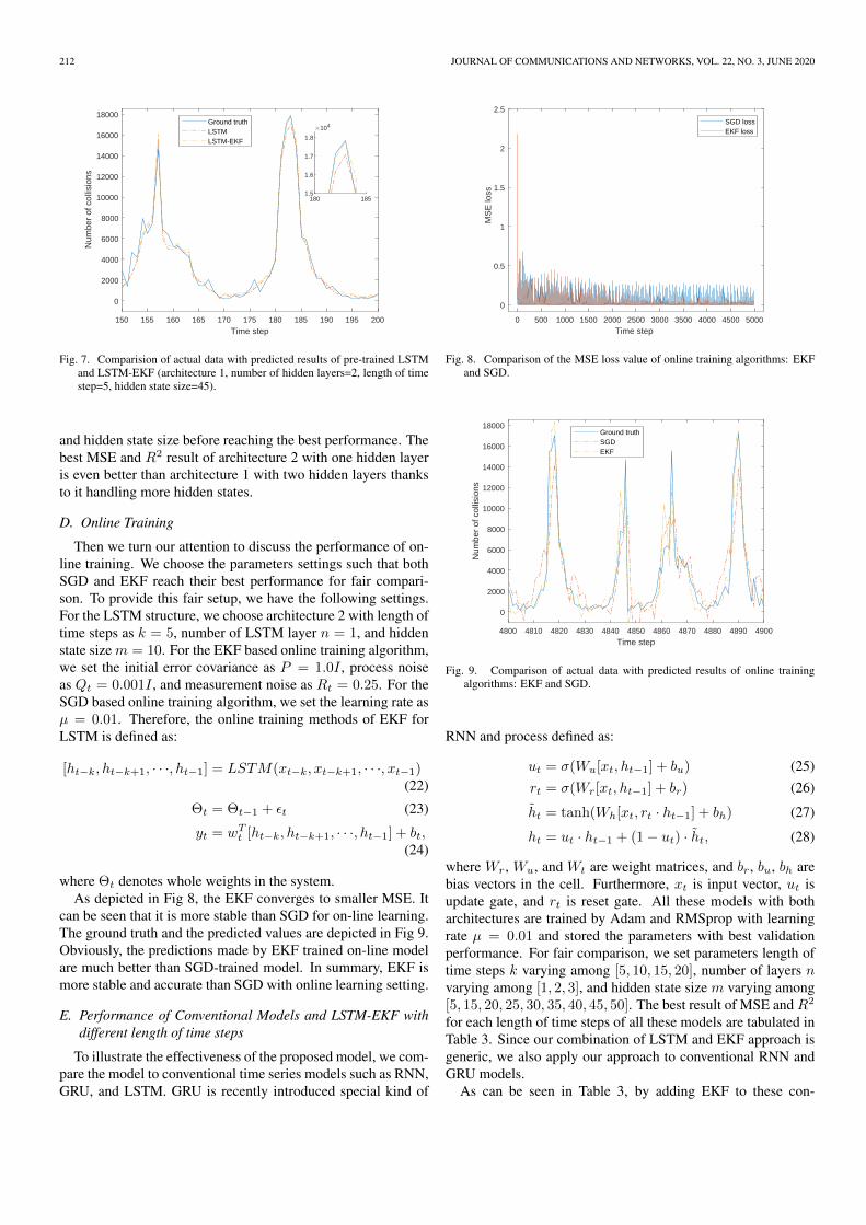
D. Online Training

Then we turn our attention to discuss the performance of on-line training. We choose the parameters settings such that bothSGD and EKF reach their best performance for fair compari-son. To provide this fair setup, we have the following settings.For the LSTM structure, we choose architecture 2 with length oftime steps as k = 5, number of LSTM layer n = 1, and hiddenstate sizem = 10. For the EKF based online training algorithm,we set the initial error covariance as P = 1.0I , process noiseas Qt = 0.001I , and measurement noise as Rt = 0.25. For theSGD based online training algorithm, we set the learning rate asµ = 0.01. Therefore, the online training methods of EKF forLSTM is defined as:

[ht−k, ht−k+1, · · ·, ht−1] = LSTM(xt−k, xt−k+1, · · ·, xt−1)(22)

Θt = Θt−1 + εt (23)

yt = wTt [ht−k, ht−k+1, · · ·, ht−1] + bt,

(24)

where Θt denotes whole weights in the system.As depicted in Fig 8, the EKF converges to smaller MSE. It

can be seen that it is more stable than SGD for on-line learning.The ground truth and the predicted values are depicted in Fig 9.Obviously, the predictions made by EKF trained on-line modelare much better than SGD-trained model. In summary, EKF ismore stable and accurate than SGD with online learning setting.

E. Performance of Conventional Models and LSTM-EKF withdifferent length of time steps

To illustrate the effectiveness of the proposed model, we com-pare the model to conventional time series models such as RNN,GRU, and LSTM. GRU is recently introduced special kind of

0 500 1000 1500 2000 2500 3000 3500 4000 4500 5000Time step

0

0.5

1

1.5

2

2.5

MS

E lo

ss

SGD lossEKF loss

Fig. 8. Comparison of the MSE loss value of online training algorithms: EKFand SGD.

4800 4810 4820 4830 4840 4850 4860 4870 4880 4890 4900

Time step

0

2000

4000

6000

8000

10000

12000

14000

16000

18000

Num

ber

of c

ollis

ions

Ground truthSGDEKF

Fig. 9. Comparison of actual data with predicted results of online trainingalgorithms: EKF and SGD.

RNN and process defined as:

ut = σ(Wu[xt, ht−1] + bu) (25)rt = σ(Wr[xt, ht−1] + br) (26)

ht = tanh(Wh[xt, rt · ht−1] + bh) (27)

ht = ut · ht−1 + (1− ut) · ht, (28)

where Wr, Wu, and Wt are weight matrices, and br, bu, bh arebias vectors in the cell. Furthermore, xt is input vector, ut isupdate gate, and rt is reset gate. All these models with botharchitectures are trained by Adam and RMSprop with learningrate µ = 0.01 and stored the parameters with best validationperformance. For fair comparison, we set parameters length oftime steps k varying among [5, 10, 15, 20], number of layers nvarying among [1, 2, 3], and hidden state size m varying among[5, 15, 20, 25, 30, 35, 40, 45, 50]. The best result of MSE andR2

for each length of time steps of all these models are tabulated inTable 3. Since our combination of LSTM and EKF approach isgeneric, we also apply our approach to conventional RNN andGRU models.

As can be seen in Table 3, by adding EKF to these con-


Table 3. Best performance of proposed model and conventional models.

Models k = 5 k = 10 k = 15 k = 20

MSE(10−3) R2 MSE(10−3) R2 MSE(10−3) R2 MSE(10−3) R2

RNN 1.0820 0.98125 1.0275 0.98248 0.9924 0.98341 1.1918 0.97956RNN-EKF 1.0760 0.98136 1.0182 0.98264 0.9890 0.98346 1.1912 0.97957GRU 1.0122 0.98246 1.0335 0.98238 0.9983 0.98331 1.1346 0.98054GRU-EKF 0.9957 0.98275 1.0318 0.98240 0.9972 0.98333 1.1269 0.98067LSTM 1.0014 0.98265 0.9586 0.98365 0.9542 0.98405 0.9596 0.98354LSTM-EKF 0.9863 0.98291 0.9475 0.98384 0.9363 0.98435 0.9437 0.98381

ventional models the results are improved. When k among[5, 10, 15], the MSE of RNN and LSTM decrease as k increases.However, when k = 20, the accuracy of RNN and LSTM bothdecrease. GRU and GRU-EKF also achieve their best perfor-mance at k = 15. For each k, the performance of LSTM modelis the best in the conventional time series models and the resultsof RNN and GRU are close. Our proposed LSTM-EKF modelachieves the best results in every different k thanks to the per-formance of LSTM backbones. Finally, since the LSTM-EKFachieves its best performance at k = 15, it is a reasonable set-tings for this prediction task.

VI. CONCLUSION

Deep learning is widely used in various industries with itspowerful learning ability. However, in the field of IoT, espe-cially the LPWAN that particularly sensitive to resource alloca-tion, how to apply deep learning is worthy of further study. Inthis paper, we studied the collision problem in LPWAN system.We then propose LSTM-EKF model for this task. We also testwith offline trained model and online trained model. Althoughoffline trained model is much more accurate than online model,it learns the pattern or the distribution of current data. On theother hand, online trained model is more adaptable for changesof patterns but not stable as offline. However, we can see thatEKF is much better than first-order gradient-based methods fortraining an online model. This model is much more stable thanonline model and can adapt to new subtle changes due to theEKF updating the parameters mapping hidden states to predictresults and freeze weights of hidden layers. Based on our pro-posed prediction models, developers or network administratorscan make pre-judgments and deal with allocation managementproblems. In the future, we would consider to construct a deeplearning based resource allocation algorithms for LPWAN sys-tem.

REFERENCES[1] A. Al-Fuqaha et al., “Internet of things: A survey on enabling technolo-

gies, protocols, and applications,” IEEE Commun. Surveys Tuts., vol. 17,no. 4, pp. 2347–2376, June 2015.

[2] L. Da Xu, W. He, and S. Li, “Internet of things in industries: A survey,”IEEE Trans. Ind. Informat., vol. 10, no. 4, pp. 2233–2243, Jan. 2014.

[3] A. Zanella et al., “Internet of things for smart cities,” IEEE Internet ThingsJ., vol. 1, no. 1, pp. 22–32, Feb. 2014.

[4] F. Tong et al., “A Tractable Analysis of Positioning Fundamentals in Low-Power Wide Area Internet of Things,” IEEE Trans. Veh. Technol., vol. 68,no. 7, pp. 7024–7034, July 2019.

[5] U. Raza, P. Kulkarni, and M. Sooriyabandara, “Low power wide areanetworks: An overview,” IEEE Commun. Surveys Tuts., vol. 19, no. 2,pp. 855–873, Jan. 2017.

[6] X. Xiong et al., “Low power wide area machine-to-machine networks:Key techniques and prototype,” IEEE Commun. Mag. vol. 53, no. 9,pp. 64–71, Sept. 2015.

[7] J. Petajajarvi et al., “On the coverage of LPWANs: Range evaluationand channel attenuation model for LoRa technology,” in Proc. ITST, Dec.2015.

[8] O. Georgiou and U. Raza, “Low power wide area network analysis: CanLoRa scale?,” IEEE Wireless Commun. Lett., vol. 6, no. 2, pp. 162–165,Apr. 2017.

[9] LoRaWAN Specification., LoRa Alliance., CA, 2017.[10] T. Voigt et al., “Mitigating inter-network interference in LoRa networks,”

J. arXiv preprint arXiv:1611.00688, 2016.[11] G. E. P. Box et al., Time series analysis: Forecasting and ontrol, John

Wiley & Sons, 2015.[12] A. Stathopoulos and M. G. Karlaftis, “A multivariate state space approach

for urban traffic flow modeling and prediction,” Transportation ResearchPart C: Emerging Technol., vol. 11, no. 1, pp. 121–135, Apr. 2003.

[13] C. Dong et al., “A spatial–temporal-based state space approach for free-way network traffic flow modelling and prediction,” Transportmetrica A:Transport Science, vol.9935, pp. 547–560, Apr. 2015.

[14] N. Sebe et al., Machine Learning in Computer Vision, Springer, 2005.[15] C. J. Schuler et al., “A machine learning approach for non-blind image

deconvolution,” in Proc. IEEE CVPR, 2013, pp. 1067–1074.[16] A. Ganapathiraju, J. Hamaker, and J. Picone, “Hybrid SVM/HMM archi-

tectures for speech recognition,” in Proc. ICSLP, 2000, pp. 504–507.[17] L. Deng and X. Li, “Machine learning paradigms for speech recognition:

An overview,” IEEE Trans. Audio, Speech, Language Process., vol. 21,no. 5, May 2013.

[18] M. N. Wernick et al., “Machine learning in medical imaging,” IEEE SignalProcess. Mag., vol. 27, no. 4, pp. 25–38, July 2010.

[19] K. Kourou et al., “Machine learning applications in cancer prognosis andprediction,” Computational Structural Biotechnology J., vol. 13, pp. 8–17,2015.

[20] L. P. Kaelbling, L. M. Littman, and A. W. Moore, “Reinforcement learn-ing: A survey,” J. Artificial Intell. Research, vol. 4, pp. 237–285, May1996.

[21] M. Wang et al., “Machine learning for networking: Workflow, advancesand opportunities,” IEEE Network, vol. 32, no. 2, pp. 92–99, Nov. 2017.

[22] B. Mao et al., “An intelligent route computation approach based on real-time deep learning strategy for software defined communication systems,”IEEE Trans. Emerg. Topics Comput., p. 1, Feb. 2019.

[23] T. Zhou et al., “A deep-learning-based radio resource assignment tech-nique for 5G ultra dense networks,” IEEE Network, vol. 32, no. 6,pp. 28–34, Nov. 2018.

[24] S. Hochreiter and J. Schmidhuber, “Long short-term memory,” J. NeuralComput., vol. 9, no. 8, pp. 1735–1780, Nov. 1997.

[25] J. Chung et al., “Empirical evaluation of gated recurrent neural networkson sequence modeling,” arXiv preprint arXiv:1412.3555, 2014.

[26] T. Kostas M et al., “A long short-term memory deep learning network forthe prediction of epileptic seizures using EEG signals,” J. Comput. BiologyMedicine, vol. 99, pp. 24–37, Aug. 2018.

[27] X. Ma, et al., “Long short-term memory neural network for traffic speedprediction using remote microwave sensor data,” Transportation ResearchPart C: Emerging Technologies, vol. 54, pp. 187–197, May. 2015.

[28] E. Chemali et al., “Long short-term memory networks for accurate state-of-charge estimation of li-ion batteries,” IEEE Trans. Ind. Electron.,vol. 65, no. 8, pp. 6730-6739, Aug. 2018

[29] J. Haxhibeqiri et al., “LoRa Scalability: A Simulation Model Based onInterference Measurements,” J. Sensors, vol. 17, no. 6, p. 1193, May. 2017.

[30] A. Mahmood et al., “Scalability analysis of a LoRa network underimperfect orthogonality,” IEEE Trans. Ind. Informat., vol. 15, no. 3,pp. 1425–1436, Mar. 2019.

[31] M. Bor et al., “Do LoRa low-power wide-area networks scale?,” in Proc.ACM MSWiM, 2016, pp. 59–67.


[32] Z. Qin et al., “Performance analysis of clustered LoRa networks,” IEEETrans. Veh. Technol., vol. 68, no. 8, pp. 7616–7629, Aug. 2019.

[33] Y. Kawamoto et al., “Multilayer Virtual Cell-Based Resource Allocationin Low-Power Wide-Area Networks,” vol. 6, no. 6, pp. 10665–10674,Dec. 2019.

[34] B. Reynders et al., “Improving Reliability and Scalability of LoRaWANsThrough Lightweight Scheduling,” IEEE Internet Things J., vol. 5, no. 3,pp. 1830–1842, June 2018.

[35] Y. Bengio et al., “Learning long-term dependencies with gradient descentis difficult,” IEEE Trans. Neural Netw., vol. 5, no. 2, pp. 157–166, Mar.1994.

[36] P. J. Werbos, “Backpropagation through time: What it is and how to do it,”Proc. IEEE, vol. 78, no. 10, pp. 1550–1560, Oct. 1990.

[37] H. Jaeger, Tutorial on training recurrent neural networks, covering BPPT,RTRL, EKF and the" echo state network" approach, Bonn: GMD-Forschungszentrum Informationstechnik, 2002.

[38] J. A. Pérez-Ortiz et al., “Kalman filters improve LSTM network perfor-mance in problems unsolvable by traditional recurrent nets,” J. NeuralNetw., vol. 16, no. 2, pp. 241–250, Mar. 2013.

[39] F. A. Gers et al., “DEKF-LSTM,” in Proc. ESANN, pp. 369–376, 2002.[40] B. D. Anderson and J. B. Moore, Optimal filtering, Courier Corporation,

2012.[41] A. Meurer et al., “SymPy: Symbolic computing in Python,” J. PeerJ Com-

puter Science 3, vol. 3, p. e103, 2017.

Shengmin Cui received B.S. degree in Computer Sci-ence and Technology from Dalian Nationalities Uni-versity in 2010, China. He acquired his Master’s de-gree in Computer Software and Theory from YunnanUniversity in 2013, China. At present, he is pursu-ing the Ph.D. degree in Computer and Software withHanyang University, South Korea. His research focusincludes Internet of things, wireless network resourcemanagement, machine learning, deep learning and re-inforcement learning.

Inwhee Joe received the B.S. degrees in ElectronicsEngineering from Hanyang University, Seoul, SouthKorea, and the Ph.D. degree in Electrical and Com-puter Engineering from the Georgia Institute of Tech-nology, Atlanta, GA, USA, in 1998. Since 2002,he has been a Falculty Member with the Division ofComputer Science and Engineering, Hanyang Univer-sity, Seoul. His current research interests include In-ternet of things, cellular systems, wireless power com-munication networks, embedded systems, network se-curity, machine learning, and performance evalua-

tion.

collision prediction for a low power wide area network

Documents