collision avoidance systems for aerospace applicationsa decision making system for collision...
TRANSCRIPT

CRANFIELD UNIVERSITY
Hamid ALTURBEH
COLLISION AVOIDANCE SYSTEMSFOR UAS OPERATING IN CIVIL
AIRSPACE
SCHOOL OF ENGINEERING
PhD THESIS

CRANFIELD UNIVERSITY
SCHOOL OF ENGINEERING
PhD THESIS
Academic Year 2013-2014
Hamid ALTURBEH
COLLISION AVOIDANCE SYSTEMS FOR UASOPERATING IN CIVIL AIRSPACE
Supervisor: Dr. James F. Whidborne
November 2014
©Cranfield University 2014. All rights reserved. No part of this publication may bereproduced without the written permission of the copyright owner.


Õ�æk���QË @ á
�
�Ôg
��QË @ é�
��<Ë @ Õ
��.�
I would like to dedicate this thesis to my family


Acknowledgements
Firstly, I would like to express my sincere gratitude to my supervisor, Dr James Whidborne,for professional supervision and his scientific assistance, constant help, advice, guidanceand good mood during the past three years. I also wish to thank all members of the Dynam-ics, Simulation and Control group.I would like to acknowledge Andrew Berry at QinetiQ for his kind help, it is worth mention-ing that part of this thesis is a development of part of Berry’s PhD thesis at the Universityof Leicester.I would also like to acknowledge and thank the pilots at the National Flying LaboratoryCentre, Cranfield University, who were helpful in giving their experience and advice thatwere useful in achieving this thesis. In particular to Susan Szasz for the interviewing anddiscussions that were essential to achieve this thesis.Finally, my biggest thanks must go to my wonderful mother, my wife Nada, and my littledaughter Sarah.

Abstract
Operation of Unmanned Aerial Vehicles (UAVs) in civil airspace is restricted by the aviationauthorities which require full compliance with regulations that apply for manned aircraft.This thesis proposes control algorithms for a collision avoidance system that can be usedas an advisory system or a guidance system for UAVs that are flying in civil airspace undervisual flight rules. An effective collision avoidance system for the UAV should be able toperform the different functionalities of the pilot in manned aircraft. Thus, it should be ableto determine, generate, and perform safe avoidance manoeuvres. However, the capability togenerate resolution advisories is crucial for the advisory systems. A decision making systemfor collision avoidance is developed based on the rules of the air. The proposed architectureof the decision making system is engineered to be implementable in both manned aircraftand UAVs to perform different tasks ranging from collision detection to a safe avoidancemanoeuvre initiation. Avoidance manoeuvres that are compliant with the rules of the air areproposed based on pilot suggestions for a subset of possible collision scenarios. The avoid-ance manoeuvre generation algorithm is augmented with pilot experience by using fuzzylogic technique to model pilot actions in generating the avoidance manoeuvres. Hence, thegenerated avoidance manoeuvres mimic the avoidance manoeuvres of manned aircraft. Theproposed avoidance manoeuvres are parameterized using a geometric approach. An optimalcollision avoidance algorithm is developed for real-time local trajectory planning. Essen-tially, a finite-horizon optimal control problem is periodically solved in real-time henceupdating the aircraft trajectory to avoid obstacles and track a predefined trajectory. The op-timal control problem is formulated in output space, and parameterised by using B-splines.Then the optimal designed outputs are mapped into control inputs of the system by usingthe inverse dynamics of a fixed wing aircraft.


Contents
Contents ix
List of Figures xiii
List of Tables xix
1 Introduction 11.1 Motivation . . . . . . . . . . . . . . . . . . . . . . . . . . . . . . . . . . . 1
1.2 Aims and Objectives . . . . . . . . . . . . . . . . . . . . . . . . . . . . . 3
1.3 Thesis Outline . . . . . . . . . . . . . . . . . . . . . . . . . . . . . . . . . 5
1.4 Contributions to Knowledge . . . . . . . . . . . . . . . . . . . . . . . . . 5
2 Collision Avoidance Systems (CAS): Literature Review 72.1 Introduction . . . . . . . . . . . . . . . . . . . . . . . . . . . . . . . . . . 7
2.2 Collision Detection and Avoidance Process . . . . . . . . . . . . . . . . . 7
2.3 Categorization Collision Avoidance Approaches . . . . . . . . . . . . . . . 10
2.3.1 Sensing Tools . . . . . . . . . . . . . . . . . . . . . . . . . . . . . 11
2.3.2 Encounter Sensing Dimension . . . . . . . . . . . . . . . . . . . . 12
2.3.3 Encounter Current State projection . . . . . . . . . . . . . . . . . . 12
2.3.4 Collision Threat Assessment . . . . . . . . . . . . . . . . . . . . 13
2.3.5 Avoidance Trajectories Calculation . . . . . . . . . . . . . . . . . 13
2.3.6 Manoeuvre Realization . . . . . . . . . . . . . . . . . . . . . . . . 14
2.3.7 Other Design Factors . . . . . . . . . . . . . . . . . . . . . . . . . 14
2.4 Collision Avoidance Approaches . . . . . . . . . . . . . . . . . . . . . . . 15
2.4.1 Predefined Collision Avoidance . . . . . . . . . . . . . . . . . . . 15
2.4.2 Protocol Based Decentralized Collision Avoidance . . . . . . . . . 15
2.4.3 Optimized Escape Trajectory Approaches . . . . . . . . . . . . . . 15
2.4.4 Potential Field Methods . . . . . . . . . . . . . . . . . . . . . . . 16
x Contents
2.4.5 Geometric Methods . . . . . . . . . . . . . . . . . . . . . . . . . . 17
2.4.6 Other CAS Approaches . . . . . . . . . . . . . . . . . . . . . . . . 17
2.5 UAS Integration in the Civil Airspace . . . . . . . . . . . . . . . . . . . . 18
2.5.1 See-and-Avoid Requirements . . . . . . . . . . . . . . . . . . . . 18
2.5.2 Related Previous and Current Research Programs . . . . . . . . . . 21
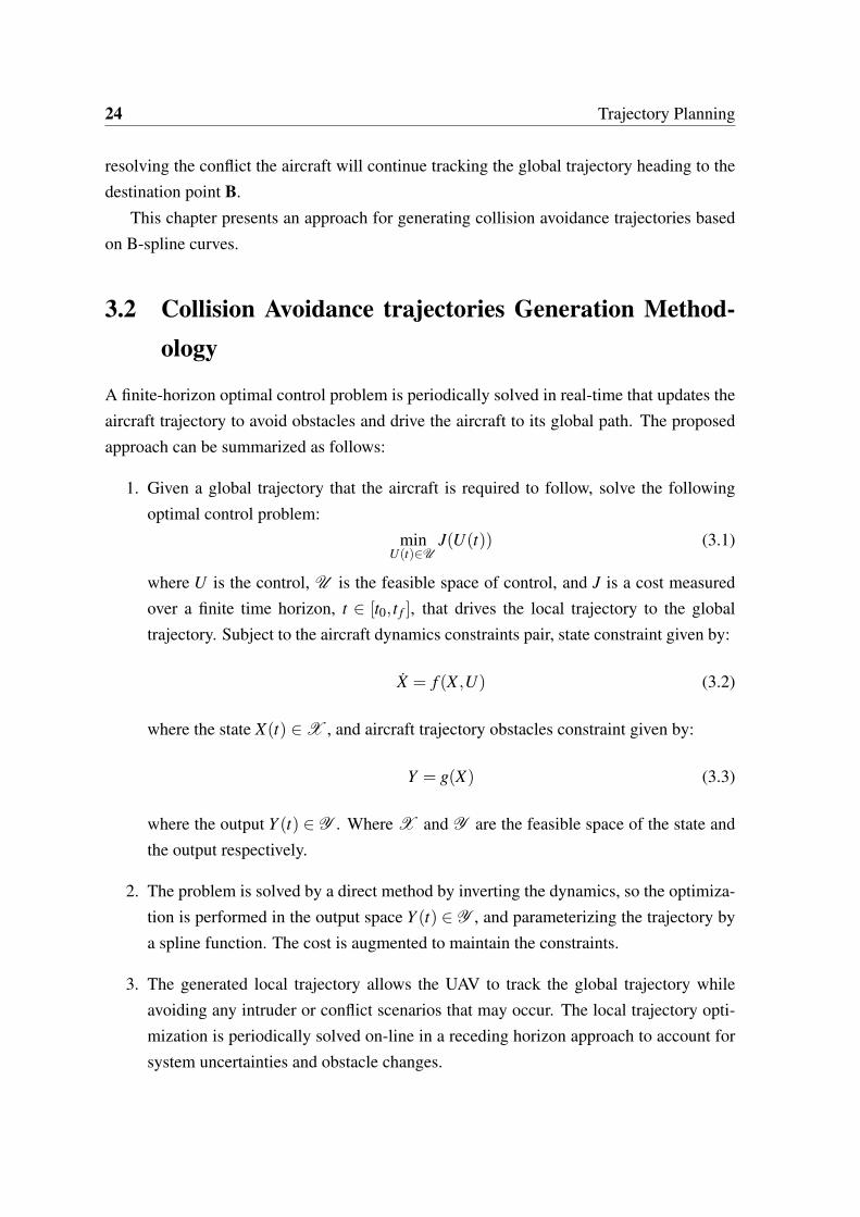
3 Trajectory Planning 233.1 Introduction . . . . . . . . . . . . . . . . . . . . . . . . . . . . . . . . . . 23
3.2 Collision Avoidance trajectories Generation Methodology . . . . . . . . . . 24
3.3 Guidance and Control Systems Architecture . . . . . . . . . . . . . . . . . 25
3.4 Local Trajectory Description . . . . . . . . . . . . . . . . . . . . . . . . . 27
3.5 B-Spline Curves . . . . . . . . . . . . . . . . . . . . . . . . . . . . . . . . 28
3.5.1 Knot Vector . . . . . . . . . . . . . . . . . . . . . . . . . . . . . . 30
3.5.2 B-spline Curves Properties . . . . . . . . . . . . . . . . . . . . . . 31
3.5.3 Derivatives of B-Spline Curves . . . . . . . . . . . . . . . . . . . . 34
3.6 Bezier Curve . . . . . . . . . . . . . . . . . . . . . . . . . . . . . . . . . 35
3.6.1 Trajectory Profiles Description Using Polynomial Functions . . . . 37
3.6.2 Boundary Conditions . . . . . . . . . . . . . . . . . . . . . . . . 39
3.7 Local Trajectory Optimisation . . . . . . . . . . . . . . . . . . . . . . . . 40
3.7.1 Differential Flatness of the Fixed-Wing Aircraft . . . . . . . . . . . 40
3.7.2 Aircraft Constraints . . . . . . . . . . . . . . . . . . . . . . . . . . 43
3.7.3 Obstacle Constraints . . . . . . . . . . . . . . . . . . . . . . . . . 44
3.7.4 Total Cost Function . . . . . . . . . . . . . . . . . . . . . . . . . . 45
3.7.5 Avoiding Local Minima . . . . . . . . . . . . . . . . . . . . . . . 46
3.8 Simulation Results . . . . . . . . . . . . . . . . . . . . . . . . . . . . . . 47
3.8.1 Global Trajectory Tracking with Static Obstacle Avoidance . . . . . 47
3.8.2 Global Trajectory Tracking with Two Moving Intruders . . . . . . . 51
3.9 Summary . . . . . . . . . . . . . . . . . . . . . . . . . . . . . . . . . . . 54
4 Decision Making System Based on The Rules of the Air 554.1 Introduction . . . . . . . . . . . . . . . . . . . . . . . . . . . . . . . . . . 55
4.2 Airspace Classification . . . . . . . . . . . . . . . . . . . . . . . . . . . . 56
4.3 Collision Avoidance in the Air . . . . . . . . . . . . . . . . . . . . . . . . 58
4.4 Right of Way Rules . . . . . . . . . . . . . . . . . . . . . . . . . . . . . . 59
4.5 The Rules of the Air for Collision Avoidance in Different Collision Scenarios 59
4.5.1 Head-on Conflict Sub-scenarios . . . . . . . . . . . . . . . . . . . 61
Contents xi
4.5.2 Converging Conflict Sub-scenarios . . . . . . . . . . . . . . . . . . 64
4.5.3 Overtaking Conflict Sub-scenarios . . . . . . . . . . . . . . . . . . 64
4.6 CAA Policy on Detect and Avoid . . . . . . . . . . . . . . . . . . . . . . . 67
4.6.1 Separation Assurance and Collision Avoidance Elements . . . . . . 67
4.6.2 Factors for Consideration when Developing a Detect and Avoid Sys-tem for UAS . . . . . . . . . . . . . . . . . . . . . . . . . . . . . 68
4.7 UAS Flight Control Mode . . . . . . . . . . . . . . . . . . . . . . . . . . 70
4.8 Decision Making System (DMS) for CAS . . . . . . . . . . . . . . . . . . 70
4.8.1 Collision Detection Layer . . . . . . . . . . . . . . . . . . . . . . 72
4.8.2 Prioritizing . . . . . . . . . . . . . . . . . . . . . . . . . . . . . . 73
4.8.3 Displaying Conflicts Data . . . . . . . . . . . . . . . . . . . . . . 76
4.8.4 Collision Assessment Layer . . . . . . . . . . . . . . . . . . . . . 78
4.8.5 Advisory System . . . . . . . . . . . . . . . . . . . . . . . . . . . 84
4.8.6 Avoidance Manoeuvre Generation . . . . . . . . . . . . . . . . . . 88
4.9 Summary . . . . . . . . . . . . . . . . . . . . . . . . . . . . . . . . . . . 88
5 Avoidance Manoeuvre Generation 895.1 Introduction . . . . . . . . . . . . . . . . . . . . . . . . . . . . . . . . . . 89
5.2 Avoidance Manoeuvre Trajectory Generation . . . . . . . . . . . . . . . . 90
5.2.1 Coordinated Turn with Constant Speed and Altitude . . . . . . . . 90
5.2.2 Avoidance Manoeuvre for Head-on/Overtaking Conflict Scenarios . 93
5.2.3 Avoidance Manoeuvre for Approaching Scenarios . . . . . . . . . 98
5.3 Avoidance Manoeuvre Parameterisation . . . . . . . . . . . . . . . . . . . 101
5.3.1 RSL Avoidance Manoeuvre Parameterisation . . . . . . . . . . . . 101
5.3.2 RS-LS Avoidance Manoeuvre Parameterisation . . . . . . . . . . . 104
5.3.3 Circle Avoidance Manoeuvre Parameterisation . . . . . . . . . . . 105
5.4 Avoidance Manoeuvre Trajectory Profiles Generation and Parameterisation 108
5.4.1 Avoidance Manoeuvre Trajectory Profiles Curve Fitting . . . . . . 110
5.5 Simulation Results . . . . . . . . . . . . . . . . . . . . . . . . . . . . . . 114
5.5.1 Head-on Scenario Simulation Results . . . . . . . . . . . . . . . . 114
5.5.2 Right Approaching Conflict Scenario Simulation Results (RSL ma-noeuvre) . . . . . . . . . . . . . . . . . . . . . . . . . . . . . . . 120
5.5.3 Right Approaching conflict Scenario Simulation Results (Circle Ma-noeuvre) . . . . . . . . . . . . . . . . . . . . . . . . . . . . . . . 126
5.6 Summary . . . . . . . . . . . . . . . . . . . . . . . . . . . . . . . . . . . 131

xii Contents
6 Pilot Behaviour-Based Collision Avoidance Manoeuvre Generation 1336.1 Introduction . . . . . . . . . . . . . . . . . . . . . . . . . . . . . . . . . . 1336.2 Fuzzy Logic Controller Structure . . . . . . . . . . . . . . . . . . . . . . 1346.3 Pilot Behaviour During the Collision Avoidance . . . . . . . . . . . . . . . 136
6.3.1 Performing the Coordinated Level Turns . . . . . . . . . . . . . . . 1376.3.2 Avoidance Manoeuvre Bank Angle Selection . . . . . . . . . . . . 1386.3.3 Avoidance Manoeuvre Roll Rate Calculation . . . . . . . . . . . . 138
6.4 Avoidance Manoeuvre Parameterisation . . . . . . . . . . . . . . . . . . . 1416.5 Simulation Results . . . . . . . . . . . . . . . . . . . . . . . . . . . . . . 148
6.5.1 Constant V with Different Values of Tc . . . . . . . . . . . . . . . 1496.5.2 Constant Tc with Different Values of V . . . . . . . . . . . . . . . 155
6.6 Summary . . . . . . . . . . . . . . . . . . . . . . . . . . . . . . . . . . . 161
7 Conclusions and Recommendations for Future Work 1637.1 Local Trajectory Planning Algorithm . . . . . . . . . . . . . . . . . . . . . 1637.2 Decision Making System . . . . . . . . . . . . . . . . . . . . . . . . . . . 1657.3 Collision Avoidance Manoeuvre Generation . . . . . . . . . . . . . . . . . 1677.4 Pilot Behaviour-Based Collision Avoidance Manoeuvre Generation . . . . . 168
Bibliography 171
Appendix A Least Squares Bezier Curve-fit 179
Appendix B Summery of Extended Interviews and Discussions with a Pilot 181
List of Figures
2.1 Collision avoidance process . . . . . . . . . . . . . . . . . . . . . . . . . 9
2.2 Current state projection methods . . . . . . . . . . . . . . . . . . . . . . . 13
3.1 Simple flight scenario: Global and local trajectories . . . . . . . . . . . . . 23
3.2 Architecture of vehicle guidance and control functionality . . . . . . . . . 26
3.3 Five segments of quadratic polynomials that join at breakpoints . . . . . . 29
3.4 B-spline basis function p=2 with open uniform knot vector . . . . . . . . . 31
3.5 Convex hull property of B-spline curve . . . . . . . . . . . . . . . . . . . 33
3.6 A quadratic curve p = 2 with cusp . . . . . . . . . . . . . . . . . . . . . . 33
3.7 Cusp removing by reallocating the control point . . . . . . . . . . . . . . 34
3.8 Bezier curve(upper), and its basis functions (lower) . . . . . . . . . . . . . 36
3.9 Aircraft point-mass model . . . . . . . . . . . . . . . . . . . . . . . . . . 40
3.10 Yukawa potential function . . . . . . . . . . . . . . . . . . . . . . . . . . 44
3.11 Block diagram of the proposed CAS . . . . . . . . . . . . . . . . . . . . . 47
3.12 Converging to the global trajectory and avoiding a static obstacle . . . . . . 48
3.13 Position, speed, ψ , and γ state during the avoidance manoeuvre (static ob-stacle) . . . . . . . . . . . . . . . . . . . . . . . . . . . . . . . . . . . . . 48
3.14 Load factor during the avoidance manoeuvre . . . . . . . . . . . . . . . . . 49
3.15 Scaling factors effects on the generated trajectory (view 1) . . . . . . . . . 50
3.16 Scaling factors effects on the generated trajectory (view 2) . . . . . . . . . 50
3.17 Collision avoidance of two scenarios, head-on (intruder1), overtaking (in-truder2) . . . . . . . . . . . . . . . . . . . . . . . . . . . . . . . . . . . . 52
3.18 Position, speed, ψ , and γ state variables during the avoidance manoeuvre . 52
3.19 Load factor during the avoidance manoeuvre . . . . . . . . . . . . . . . . . 53
3.20 UAV-intruder1 distance (upper), UAV-intruder2 distance (lower) . . . . . . 53
4.1 UK airspace classification . . . . . . . . . . . . . . . . . . . . . . . . . . . 57
xiv List of Figures
4.2 Fixed position of another aircraft in the windscreen indicates a constant rel-ative bearing and therefore a collision risk . . . . . . . . . . . . . . . . . . 59
4.3 Rules of right of way around the aircraft . . . . . . . . . . . . . . . . . . . 60
4.4 Head-on case: Both aircraft should turn right . . . . . . . . . . . . . . . . 60
4.5 Overtaking scenario: The overtaken aircraft (B) will continue straight whilethe overtaking aircraft (A) must turn right . . . . . . . . . . . . . . . . . . 61
4.6 Converging case: Aircraft B has the right of way . . . . . . . . . . . . . . 61
4.7 Head-on collision scenario (a) no offset; (b) offset exists . . . . . . . . . . 62
4.8 Head-on scenario in which both aircraft are descending . . . . . . . . . . . 62
4.9 Head-on scenario where the both aircraft are climbing . . . . . . . . . . . 63
4.10 Head-on scenario: One vehicle is in level flight and the other is climbing . 63
4.11 Head-on scenario: One aircraft is in level flight and the other is descending 63
4.12 Converging conflict with resolution manoeuvres . . . . . . . . . . . . . . . 64
4.13 Overtaking conflict scenario: Both aircraft are in level flight, no offset (a);offset exists (b) . . . . . . . . . . . . . . . . . . . . . . . . . . . . . . . . 65
4.14 Overtaking conflict scenario: Both aircraft are descending . . . . . . . . . 65
4.15 Overtaking conflict scenario: Both aircraft are climbing . . . . . . . . . . . 66
4.16 Overtaking conflict scenario:The overtaking aircraft is in level flight, andthe overtaken aircraft is climbing . . . . . . . . . . . . . . . . . . . . . . . 66
4.17 Overtaking conflict scenario: The overtaking aircraft is climbing, and theovertaken aircraft is in level flight . . . . . . . . . . . . . . . . . . . . . . 66
4.18 Overtaking conflict scenario: The overtaking aircraft is in level flight, andthe overtaken aircraft is descending . . . . . . . . . . . . . . . . . . . . . . 67
4.19 Overtaking conflict scenario:The overtaking aircraft is descending, and theovertaken aircraft is in level flight . . . . . . . . . . . . . . . . . . . . . . 67
4.20 DMS architicture . . . . . . . . . . . . . . . . . . . . . . . . . . . . . . . 71
4.21 Range, and relative altitude: Horizontal plane (upper); Vertical plane (lower) 73
4.22 Flowchart of the collision detection system . . . . . . . . . . . . . . . . . 74
4.23 Three intruders scenario with different priorities (Horizintal plane (upper)shows the ranges; Vertical plane (lower) shows the relative altitudes . . . . 75
4.24 Conflict scenario clarifying the importance of the Tc in the prioritizing pro-cess . . . . . . . . . . . . . . . . . . . . . . . . . . . . . . . . . . . . . . 77
4.25 PCAS XRX . . . . . . . . . . . . . . . . . . . . . . . . . . . . . . . . . . 78
4.26 PCAS XRX display . . . . . . . . . . . . . . . . . . . . . . . . . . . . . . 78
4.27 Displaying Layer-1 output on GUI/ Avionics . . . . . . . . . . . . . . . . 79

List of Figures xv
4.28 Conflict scenario (left), and its displayed information on GUI/Avoinics (right) 80
4.29 Range and bearing of the aircraft and the intruder in NEU and body refer-ence frames . . . . . . . . . . . . . . . . . . . . . . . . . . . . . . . . . . 81
4.30 Collision assessment algorithm flowchart . . . . . . . . . . . . . . . . . . 81
4.31 Conflict scenario (left), GUI with Layer-1, and Layer-2 information (right) 82
4.32 Aircraft closure rate chart . . . . . . . . . . . . . . . . . . . . . . . . . . 83
4.33 Flowchart for advisory generating during head-on collision . . . . . . . . . 85
4.34 Flowchart for RA generation for overtaking/overtaken conflict scenarios . . 86
4.35 GUI/Avionics layout including the conflict resolution advisories . . . . . . 87
5.1 Forces balance in equilibrium state of turning aircraft . . . . . . . . . . . . 91
5.2 The avoidance manoeuvre for the head-on conflict scenario . . . . . . . . 94
5.3 The heading rate of the proposed head-on collision avoidance manoeuvre . 94
5.4 The heading angle of the proposed head-on collision avoidance manoeuvre 95
5.5 The geometric representation of the proposed head-on collision avoidancemanoeuvre . . . . . . . . . . . . . . . . . . . . . . . . . . . . . . . . . . 96
5.6 Avoidance manoeuvre initialization and interruption by CF, and RF . . . . 97
5.7 Avoidance manoeuvres for different right approaching conflict scenarios . 100
5.8 The RSL avoidance manoeuvre for right approaching conflict scenario . . . 101
5.9 The heading rate signal that generates the proposed RSL avoidance manoeu-vre . . . . . . . . . . . . . . . . . . . . . . . . . . . . . . . . . . . . . . 102
5.10 The heading angle of the RSL avoidance manoeuvre . . . . . . . . . . . . 102
5.11 The RS-LS avoidance manoeuvre parts sequence . . . . . . . . . . . . . . 104
5.12 The geometric representation of the proposed circle avoidance manoeuvre . 105
5.13 Heading rate for the circle avoidance manoeuvre . . . . . . . . . . . . . . 107
5.14 Heading angle for the circle avoidance manoeuvre . . . . . . . . . . . . . 107
5.15 Flowchart of discrete trajectory profiles calculation . . . . . . . . . . . . . 109
5.16 CAS Flowchart . . . . . . . . . . . . . . . . . . . . . . . . . . . . . . . . 113
5.17 Block diagram for CAS simulation . . . . . . . . . . . . . . . . . . . . . . 114
5.18 Head-on conflict scenario . . . . . . . . . . . . . . . . . . . . . . . . . . . 115
5.19 Simulation results of attitude (heading rate, heading angle, roll angle, andflight path angle) for the head-on conflict avoidance manoeuvre . . . . . . . 117
5.20 Simulation results of speeds (V , u, v , and w) for the head-on conflict avoid-ance manoeuvre . . . . . . . . . . . . . . . . . . . . . . . . . . . . . . . . 118
5.21 Load factor during the avoidance manoeuvre . . . . . . . . . . . . . . . . . 119

xvi List of Figures
5.22 3D view of the UAV trajectory for the head-on conflict avoidance manoeuvre 119
5.23 Right approaching scenario . . . . . . . . . . . . . . . . . . . . . . . . . . 121
5.24 Simulation results of attitude (heading rate, heading angle, roll angle, andflight path angle) for the RSL avoidance manoeuvre . . . . . . . . . . . . 122
5.25 Simulation results of speeds (V , u, v , and w) for the RSL avoidance manoeuvre124
5.26 Load factor during the avoidance manoeuvre . . . . . . . . . . . . . . . . . 125
5.27 3D view of the UAV trajectory for the RSL avoidance manoeuvre . . . . . 125
5.28 The circle avoidance manoeuvre for a right approaching conflict scenario . 127
5.29 Simulation results of attitude (heading rate, heading angle, roll angle, andflight path angle) for the circle avoidance manoeuvre . . . . . . . . . . . . 128
5.30 Simulation results of speeds (V , u, v , and w) for the circle avoidance ma-noeuvre . . . . . . . . . . . . . . . . . . . . . . . . . . . . . . . . . . . . 129
5.31 Load factor during the avoidance manoeuvre . . . . . . . . . . . . . . . . . 130
5.32 3D view of the UAV trajectory for the circle avoidance manoeuvre . . . . . 130
6.1 Mamdani fuzzy logic system . . . . . . . . . . . . . . . . . . . . . . . . . 136
6.2 Time to collide membership functions . . . . . . . . . . . . . . . . . . . . 139
6.3 Speed membership functions . . . . . . . . . . . . . . . . . . . . . . . . . 139
6.4 Bank Angle (output) membership functions . . . . . . . . . . . . . . . . . 140
6.5 Roll rate φ . . . . . . . . . . . . . . . . . . . . . . . . . . . . . . . . . . . 142
6.6 Bank angle φ . . . . . . . . . . . . . . . . . . . . . . . . . . . . . . . . . 142
6.7 The heading rate . . . . . . . . . . . . . . . . . . . . . . . . . . . . . . . 143
6.8 The heading angle . . . . . . . . . . . . . . . . . . . . . . . . . . . . . . 144
6.9 Calculation of the UAV position at the end of the time period Tr . . . . . . 146
6.10 Avoidance manoeuvre generation algorithm flowchart . . . . . . . . . . . 147
6.11 System block diagram . . . . . . . . . . . . . . . . . . . . . . . . . . . . 148
6.12 Head-on conflict scenarios (1,2, and 3) . . . . . . . . . . . . . . . . . . . . 149
6.13 The simulation results of (φ , ψ , V , and altitude) for scenarios (1, 2, and 3) . 151
6.14 Scenario1 simulation results (Left): u, v, and w; (Right): ψ , φ , and γ . . . . 152
6.15 Scenario 1: 3D view of the UAV, and the intruder trajectories . . . . . . . . 152
6.16 Scenario2 simulation results (Left): u, v, and w; (Right): ψ , φ , and γ . . . . 153
6.17 Scenario 2: 3D view of the UAV, and the intruder trajectories . . . . . . . . 153
6.18 Scenario3 simulation results (left): u, v, and w; (Right): ψ , φ , and γ . . . . 154
6.19 Scenario 3: 3D view of the UAV, and the intruder trajectories . . . . . . . . 154

List of Figures xvii
6.20 The UAV trajectories in horizontal plane for the conflict scenarios (1, 2, and3) . . . . . . . . . . . . . . . . . . . . . . . . . . . . . . . . . . . . . . . 155
6.21 Head-on conflict scenarios (4,5, and 6) . . . . . . . . . . . . . . . . . . . . 1556.22 The simulation results of (φ , ψ , V , and altitude) for scenarios (4, 5, and 6) . 1576.23 Scenario4 simulation results (left): u, v, and w; (Right): ψ , φ , and γ . . . . 1586.24 Scenario 4: 3D view of the UAV, and the intruder trajectories . . . . . . . . 1586.25 Scenario5 simulation results (left): u, v, and w; (Right): ψ , φ , and γ . . . . 1596.26 Scenario 5: 3D view of the UAV, and the intruder trajectories . . . . . . . . 1596.27 Scenario6 simulation results (left): u, v, and w; (Right): ψ , φ , and γ . . . . 1606.28 Scenario 6: 3D view of the UAV, and the intruder trajectories . . . . . . . . 1606.29 The UAV trajectories in the horizontal plane for the conflict scenarios (4, 5,
and 6) . . . . . . . . . . . . . . . . . . . . . . . . . . . . . . . . . . . . . 161


List of Tables
3.1 Scaling factors values . . . . . . . . . . . . . . . . . . . . . . . . . . . . . 49
4.1 Flight Control Mode for UAS Class Ratings . . . . . . . . . . . . . . . . . 70
5.1 Average and exaggerated manoeuvre quantities . . . . . . . . . . . . . . . 98
6.1 Fuzzy inference engine (the aircraft starts manoeuvreing first) . . . . . . . 1406.2 Fuzzy inference engine (the intruder starts manoeuvreing first) . . . . . . . 1416.3 Conflict scenarios (1,2, and 3): V =Vi = 50m.s−1, ∆ψ = 60o, φ = 45o . . . 1496.4 Simulation scenarios: Ra = 2500m, ∆ψ = 60o, φ = 45o . . . . . . . . . . . 156

Nomenclature
List of Symbols
α Decay rate of the Yukawa potential function
B Discretised basis functions matrix
Bls Curve fit matrix
C Curve coefficient matrix matrix
φ Roll rate
ψ Heading rate
γ Flight path angle
λ Scaling factor
φ Bank angle
ψ Heading angle
ρ Air density
τ Curve parameter
Bi ith order basis function
CD Drag coefficient
Ci Coefficient for each of the ith order basis functions
CL Lift coefficient
CD0 Minimum drag coefficient
xxii Nomenclature
D Drag
dc Clearance distance
g Gravity acceleration
J Cost function
L Aircraft lift
m Aircraft total mass
n Load factor
Ni,p The pth degree B-spline basis functions
P(τ) Polynomial curve description as a function of τ
R Turn radius
Ri,p The ith order rational basis function of degree p
S Wing area
T Thrust
t Time
Tc Time to collision
th Time horizon
Tm Manoeuvre time
Ts Sampling time
U Knot vector: Control vector
u UAV speed on x-axis in earth reference frame
V Aircraft speed
v UAV speed on y-axis in earth reference frame
Vstallturn Stall speed in the turn
Nomenclature xxiii
Vstall Stall speed
w UAV speed on z-axis in earth reference frame
wi Weights
x,y,z Aircraft center of gravity coordinates in earth axis
xxiv Nomenclature
List of Acronyms
ADR Advisory Routes
ADS Advisory System
ADS-B Automatic Dependent Surveillance-Broadcast
AF Alert Flag
AFRL Air Force Research Laboratory
AMG Avoidance Manoeuvre Generator
AOUAV Autonomously Operating Unmanned Aerial Vehicle
ASAS Airborne Separation Assistance System
ASTRAEA Autonomous System Technology Related Airborne Evaluation andAssessment
ATC Air Traffic Controller
ATZ Aerodrome Traffic Zones
CA Collision Assessment
CAA Civil Aviation Authority
CDP Collision Detection and Prioritizing
CDR Conflict Detection and Resolution
CF Collision Flag
CTR Aerodrome Control Zone
DCM Directional Cosine Matrix
ELOS Equivalent Level of Safety
FAA Federal Aviation Administration
FCM Flight Control Modes
Nomenclature xxv
FLC Fuzzy Logic Control
GPS Global Positioning System
GPWS Ground Proximity Warning System
GUI Graphic User Interface
HMI Human Machine Interface
IFR Instrument Flight Rules
LTP Local Trajectory Planner
MIDCAS Mid Air Collision Avoidance System
MPC Model Predictive Control
MPC Model Predictive Control
NAS National Airspace System
NEU North, East, Up
NF Nine O’clock Flag
NURBS Non-uniform Rational B-Spline
OODA Observe, Orient, Decide, and Act
PCAS Portable Collision Avoidance System
PZ Protected Zone
RA Resolution Advisories
RF Collision Resolved Flag
RHC Receding Horizon Control
RS-LS Right-Straight then Left-Straight
RSL Right-Straight-Left
SAA Sense and Avoid

xxvi Nomenclature
SAAFT Sense and Avoid Flight Tests
TCAS Traffic Alert and Collision Avoidance System
TMA Terminal Control Area
UAS Unmanned Aircraft Systems
UAV Unmanned Aerial Vehicle
VFR Visual Flight Rules
VMC Visual Meteorological Conditions

Chapter 1
Introduction
1.1 Motivation
Unmanned Aircraft Systems (UAS) are of increasing importance in the aerospace indus-try for both civilian and military applications due to their ability to complete dull, dirtyand dangerous missions [1]. However, operation of Unmanned Aerial Vehicles (UAV’s) incivil/non-segregated airspace is restricted by the policies of aviation authorities (e.g. CivilAviation Authority (CAA) in the UK, Federal Aviation Administration (FAA) in the USA),which require full compliance with rules and obligations that apply for manned aircraft [2–4].
The development of a good Sense and Avoid (SAA) system is one of the most importantissues that a UAV designer must deal with to give the UAV the ability to avoid conflict situ-ations as required for manned aircraft. SAA capability must provide for collision avoidanceprotection between a UAS and other aircraft analogous to the see and avoid operation ofmanned aircraft that meets an acceptable level of safety [2]. Much research is being un-dertaken to achieve the civil aviation authorities requirements for SAA system, and henceenable the routine use of UAV’s in all classes of airspace without the need for restrictiveor specialized conditions of operation [3, 51? ]. However, significant progress is only ex-pected in the mid-term (between 2015-2020), and a standardised SAA system is expected tobe achieved after 2020. These expectations have been made by the FAA (Integration of CivilUnmanned Aircraft Systems (UAS) in the National Airspace System (NAS) Roadmap) dueto the complexity of SAA concepts, and the immature development of SAA technology [2].
The lack of a SAA system to avoid collisions with other aircraft is a major barrier to

2 Introduction
UAS operations in non-segregated and civil airspace [5]. The operation of a SAA systemcan be considered in three levels [3]:
1. Strategic SAA: Conflict to be detected at long range, so the system can maintain sep-aration distance by adjusting the UAS trajectory. Hence, collisions will not happen.
2. Conflict Resolution Advisories (RA): These advisories are issued to the UAV pilot(UAVp) to avoid collisions based on the rules of the air. The RA must be accepted bythe UAVp before a manoeuvre is executed.
3. Autonomous collision avoidance: UAV avoids the collision autonomously.
In a manned aircraft the pilot in command has the ultimate responsibility for achievingthe collision avoidance manoeuvre using the see and avoid principle. The pilot’s decisionprocess during the conflict can be broken down using the Observe, Orient, Decide, and Act(OODA) loop [3, 6]:
• Observe: A pilot visually scans for collision threats. Information that is offered byAir Traffic Controller (ATC), or the aircraft avionics helps the pilot to detect potentialcollision threats.
• Orient: Pilot uses his/her knowledge and experience to evaluate what is seen. Thus,the range, speed, and bearing of the threats can be estimated based on apparent sizegrowth, and the assumptions about the threat type.
• Decide: The pilot should determine a safe avoidance manoeuvre that will be per-formed in order to avoid the collision safely. The avoidance manoeuvre should becompliant with the rules of the air.
• Act: Finally, the determined safe manoeuvre is performed by the pilot.
The required time for a pilot to recognise an approaching aircraft and initiate an avoidancemanoeuvre is 12.5 seconds in total [7]. Most of this time is spent on collision recognitionand decision making (See Section 4.8.4). However, this time may be greater because pi-lots differ in their response time [8]. Hence, a Decision Making System (DMS) that couldbe used as an advisory system will effectively save time and help both the on-board pilotin manned aircraft, and the UAV ground-based pilot to avoid the conflicts safely. In anAutonomously Operating UAV (AOUAV) the DMS could be used to initiate avoidance ma-noeuvres.

1.2 Aims and Objectives 3
The motivation of this thesis is to develop a collision avoidance system that is able toissue the resolution advisories, and generate and track safe avoidance manoeuvres. Thesemanoeuvres should be similar to those performed by a pilot in manned aircraft which arecompliant with the rules of the air.
1.2 Aims and Objectives
This thesis aims to develop a control algorithm for collision avoidance system for aircraftthat fly under Visual Flight Rules (VFR) conditions. This algorithm could be used as anadvisory system for manned aircraft, or a guidance system for UAV in order to enable flightin civil airspace. According to the policies of civil aviation authorities around the world theUAV operating in civil airspace must satisfy the safety and operational conditions at least asmanned aircraft [9]. So a UAV that behaves the same as manned aircraft in all conditionsmeans an aircraft that is in full compliance with air traffic rules.
The manoeuvre during conflict resolution is a very important issue in Collision Avoid-ance Systems (CAS). Hence, this thesis investigates trajectory optimisation during the ma-neuvers, as well as the air traffic rules satisfaction for a subset of the possible conflict sce-narios.
The capability of RA generation, and a safe avoidance manoeuvre determination neces-sitates a type of decision making algorithm that is able to perform the different functionali-ties of the pilot in manned aircraft. The aim here is to develop an architecture of the DMSthat can be implementable in manned and unmanned aircraft, taking into consideration thecivil aviation authorities requirements.
Furthermore, it is sometimes difficult to model pilot behaviour using deterministic mod-els. However, the Fuzzy Logic Control (FLC) technique provides a tool for modellinghuman behaviour. The aim is to use the fuzzy logic technique to design fuzzy logic pilotmodels that express human centered rules in order to generate avoidance manoeuvres basedon the pilot experience.
These aims are achieved by the following proposed objectives:
1. Review the work carried out on CAS for the airspace application.

4 Introduction
2. Review the aviation authorities requirements and obligation for UAV integration incivil airspace.
3. Develop control algorithms for local trajectory planning. The local trajectory musttrack a predefined global trajectory and avoid any pop-up obstacles. This will include:
(a) Orthogonal basis function local trajectory generation methods (B-spline curvemethods).
(b) Avoidance manoeuvre optimisation.
4. Develop a generic Decision Making System (DMS) for collision avoidance systembased on the rules of the air in visual flight rules (VFR) conditions, and the civilaviation authorities requirements. The developed DMS should be able to perform thefollowing tasks:
(a) Conflicts detection and prioritizing.
(b) Conflicts evaluation and assessment.
(c) Issue warning alerts and conflict resolution advisories.
(d) Initiate corespondent safe avoidance manoeuvres.
5. Propose and generate collision avoidance manoeuvres that should be similar to theavoidance manoeuvres of manned aircraft (this could be carried out for a subset of theall possible conflict scenarios). This includes:
(a) Specify the type of the avoidance manoeuvres.
(b) Find the characteristics of the avoidance manoeuvres.
(c) Parameterize the avoidance manoeuvres.
6. Augment the avoidance manoeuvre generation process, so that the algorithm mimicspilot behaviour by using fuzzy logic techniques. This can be achieved by determiningthe inputs and outputs of the fuzzy logic system, and generating the fuzzy logic rulesbased on pilot behaviour during the conflict.
7. Test algorithms in simulation using MATLAB/Simulink.
1.3 Thesis Outline 5
1.3 Thesis Outline
This thesis consists of seven chapters including the introduction chapter. The remainder ofthis thesis is structured as follows:
• Chapter 2 provides a literature review of collision avoidance systems for aircraft.
• Chapter 3 presents a local trajectory planning algorithm that is used for the collisionavoidance system for a fixed-wing aircraft.
• Chapter 4 proposes a decision making system (DMS) algorithm for the collisionavoidance systems (CAS).
• Chapter 5 discusses the avoidance manoeuvres generating process for different con-flict scenarios in which the UAV should change direction (right/left turn) in horizontalplane.
• Chapter 6 discusses how pilot experience can be used in the collision avoidance ma-noeuvre generation process for the UAV.
• The conclusions, limitations of the proposed algorithms, and recommendations forfuture work are given in Chapter 7.
1.4 Contributions to Knowledge
The contributions to knowledge which have been made as part of this work are summarizedbelow:
• Develop a real-time local trajectory planning algorithm for a fixed-wing UAV using B-spline and MPC. The developed method is an extension of a previous method that wasproposed for a quad-rotor UAV [10]. The developed method uses the differential flat-ness property of the fixed-wing aircraft to develop an inverse dynamic model. Hence,mapping the generated trajectory into the UAV’s control commands is achieved. Amethod that helps the optimisation solver to avoid a local minimum is proposed.
• Develop a decision making system (DMS) architecture for collision avoidance systemin VFR conditions. The proposed DMS architecture mimics the pilot decision makingprocess during a conflict scenario. Thus, it could be used at different levels of aircraftautonomy (e.g. manned aircraft, remotely piloted UAV, or autonomously operatingUAV).
6 Introduction
• A graphical user interface (GUI) is proposed for algorithm test and simulation pur-poses with short comparison with currently used commercial Portable Collision Avoid-ance System (PCAS). The proposed GUI layout is designed based on the intruderpriority.
• Propose, construct, and parameterise collision avoidance manoeuvres for a set of con-flict scenarios:
1. Head-on/overtaking conflict scenarios.
2. Approaching conflict scenarios.
The collision avoidance manoeuvres are proposed based on pilot suggestions1. Hence,the shapes of the manoeuvres are similar to the manoeuvres that are performed bymanned aircraft.
• A pilot behavioural model is augmented in collision avoidance manoeuvres by usingfuzzy logic technique to model the pilot reaction.
• A geometric approach is proposed to parameterise the generated collision avoidancemanoeuvres. Thus the construction and generation the avoidance manoeuvres aresimplified, hence the computational time for avoidance manoeuvre generation is re-duced.
1Extended interviews and discussions about the problem have been carried out with a pilot at NationalFlying Lab, Cranfield University (See Appendix B)

Chapter 2
Collision Avoidance Systems (CAS):Literature Review
2.1 Introduction
Many studies have been carried out to solve the collision avoidance problem in airspaceto improve the performance of both Conflict Detection and Resolution (CDR) for mannedand unmanned vehicles. For manned aircraft, the human element is key in the collisionavoidance process in many methods due to the pilots ability to make decisions accordingto the collected information [11]. However, humans are prone to errors and hence auto-mated systems seem to be an alternative solution. Automated Collision Avoidance Systems(CAS) are being used as advisory systems (e.g. Traffic Alert and Collision Avoidance Sys-tem (TCAS)) in piloted aircraft but they can also be embedded with guidance systems inUAV’s [12]. More than sixty different conflict detection and resolution methods have beenaddressed in the literature, not only in aerospace applications, but also for ground vehicles,and robotics [11]. In the recent years, the development in sensors technology and powerfulprocessing units has led to a significant enhancement in both detection and resolving conflictscenarios [12].
2.2 Collision Detection and Avoidance Process
A collision or conflict can be defined as an event when there is loss in separation distancebetween two or more vehicles [13]. The distance of separation has different values depen-dening on the air traffic rules. The minimum separation distance according to traffic rules

8 Collision Avoidance Systems (CAS): Literature Review
in civil aerospace is 5 nmi and 1000 ft for horizontal and vertical distances respectively(Instrument Flight Rules (IFR)) [11]. These separation distances can be represented as avolume that surrounds each aircraft, called the Protected Zone (PZ). Hence, a conflict oc-curs, if there is any interference between these protected zones [14]. For example, in tacticalcollision alerting systems the PZ is taken as a sphere of 500 ft in diameter, or it can be rep-resented in terms of time instead of distance [11]. However, the functions of CDR systemsare the same in all cases, which are conflict prediction, provide the information to the pilot(in case of manned aircraft), or to the guidance system (in the case of autonomous UAVs),and, in some cases, evaluate the avoidance action.
Figure 2.1 shows a block diagram that simply illustrates the collision avoidance process:
1. The first step in the collision avoidance process is to monitor the traffic environmentand identify the current traffic situation. The state estimator estimates the currenttraffic situation by collecting appropriate current states that are measured by sensorsand communication equipment. However, uncertainty in measured states may occurdue to sensor errors and/or limitation of the update rate [12].
2. In order to predict a conflict in the future, a dynamic trajectory model is required asshown in Figure 2.1; this block projects the current states into the future. This pro-jection may be based solely on current state information. For example, a straight-lineextrapolation of the current velocity vector, or may be based on additional, proceduralinformation such as a flight plan [11]. Furthermore, due to model uncertainty, there isalso a mismatch between the estimated trajectory and actual one.
3. The current and estimated states are combined to calculate some metrics to maketraffic management decisions. Some examples of metrics include predicted mini-mum separation, and the estimated time to closest point of approach. In the trafficenvironment, the current and projected states can be calculated separately for eachaircraft. However, the metric aggregates information from the aircraft that share thesame airspace in order to manage the traffic situation.
4. The Conflict detection block then uses the conflict metrics to decide whether alarmshould be issued and whether action is needed to avoid the conflict. However, inmany cases of piloted aircraft, the pilot determines the appropriate actions in orderto avoid collision. So in this case the function of the CDR system is just to issue thenotifications of conflict [11].

2.2 Collision Detection and Avoidance Process 9
Environment contains static
and moving objects
State Estimation
Dynamic Model
Metric Defintion
Conflict ResolutionConflict Detection
Human Operator
(Manned Aircraft)
Guidance System (UAV)
Cu
rre
nt
Sta
tes
Pro
jecte
d
Sta
tes
Metrics
Figure 2.1 Collision avoidance process
The CDR systems in a UAV has different functions. In addition to conflict predictionit also resolves the conflict by using collision avoidance algorithms. It is worth mentioningthat the notification or action will not be issued for all predicted conflicts because there aresome predicted conflicts that are far into the future or too uncertain [11]. The resolutionstage operates when the action to avoid the collision becomes necessary. The function ofthe conflict resolution stage can be expressed either as an advisory system such as TCAS,which gives the pilot appropriate commands that are needed to avoid the conflict, or as afeedback system that gives the ability to the operator to monitor if their action will resolvethe conflict or not. This kind of system can be categorised as a passive system [15].

10 Collision Avoidance Systems (CAS): Literature Review
The conflict resolution block in Figure 2.1 has an independent state estimator, model ofmanoeuvre trajectory, and decision criteria. Either or both collision detection and collisionavoidance may be automated or may be handled manually through procedures. For instance,the pilot is responsible for conflict detection and resolution in Visual Flight Rules (VFR),so the pilot must scan traffic visually (conflict detection) and take suitable action (basedon the rules of the air) if there is a threat of collision (conflict avoidance) [16]. However,Instrument Flight Rules (IFR) place responsibility for monitoring the traffic separation onthe Air Traffic Controller (ATC) who is using radar to detect the traffic separation, and issuesresolutions to aircraft if a conflict threat is detected. In case of the aircraft that is equippedwith an airborne CAS (e.g. TCAS), if operators fail to resolve the collision, additionalguidance information is issued by TCAS [15]. One reason that makes the CDR systemchallenging and interesting is that there is interdependence between conflict detection andconflict resolution. As it is not easy to isolate conflict detection from conflict resolution andvice versa, there are many feasible design solutions. For example, deciding when actionis required to resolve the conflict may depend on the action type, and similarly the type ofrequired action may depend on how early that action begins [11].
2.3 Categorization Collision Avoidance Approaches
To provide insight into different CDR approaches, all different proposed methods must becategorized. The categorization should be built on fundamental factors that can express andidentify the differences between each method. A good illustration of the design factors isgiven in [13] and [11] that are:
• Sensing tools,
• Encounter sensing dimension,
• Encounter current states projection,
• Collision threat assessment,
• Avoidance trajectories calculation and,
• Manoeuvre realization, and other design factors.
The next subsections give further detail of each design factor.
2.3 Categorization Collision Avoidance Approaches 11
2.3.1 Sensing Tools
The traffic environment information around aircraft is collected by using sensors. The col-lected information by the sensors is used by automated systems to predict the conflict sce-nario which may use this prediction in the guidance algorithms to avoid conflict. The sensorsthat are used in CDR system can be divided into two main categories: cooperative and non-cooperative traffic sensors.
Cooperative traffic sensors enable aircraft to share information such as speed, heading,and position with other aircraft and airspace traffic control (ATC). Examples of cooperativetraffic sensors are: Airborne Separation Assistance System (ASAS), and Automatic Depen-dant Surveillance Broadcast (ADS-B). These transfer aircraft information to ATC and otheragents.
Aircraft that are not equipped with cooperative traffic sensors get information aboutsurrounding airspace by using non-cooperative traffic sensors. There are different typesof sensors that can sense the surrounding environment and collect information about otheraircraft in shared airspace. Laser range finder, Electro-Optical/Infra-Red (EO/IR), radar sys-tem, stereo camera pairs, and moving single camera are some examples of sensors that areused in non-cooperative traffic systems[17–19]. However, non-cooperative sensor systemshave their limitations. For example, the laser range finders, which are effective in detectingscanned obstacles, have limited capabilities to detect the environment and they are relativelyexpensive. Although radar systems can detect moving and stationary obstacles effectively,their weight and size mean their use in a small UAV is limited. The recent advances of dig-ital signal processors have enabled the use of cameras as passive sensors that can provideinformation about the surrounding environment. Much research has already been conductedto use cameras in CAS systems [20, 21]. However experimental research carried out by [22],has shown a poor result for camera systems compared with humans in terms of detectingthe intruder aircraft. The data accuracy that is provided by sensors is limited and dependson sensor type. The density of received data and data update rate add further limitations ofdata processing and uncertainty. One way to avoid failures associated with these limitationsis increasing the safety distance between aircraft [12].

12 Collision Avoidance Systems (CAS): Literature Review
2.3.2 Encounter Sensing Dimension
The surrounding environment can be described either in a two dimensional plane (2D), or athree dimensional space (3D). The two dimensional approach can be either two dimensionalhorizontal plane (2D-H), or two dimensional vertical plane (2D-V). Most CAS can be cat-egorized under 3D, or 2D-H approaches. However, the Ground Proximity Warning System(GPWS) uses a 2D-V approach [23].
2.3.3 Encounter Current State projection
Future prediction is one of the main componants of CAS by specifying how to projectthe current states of UAV and encounter into the near future, so the conflict threat can beassessed. Figure 2.2 shows four different methods for prediction which are [13]:
1. Straight projection (2.2 A): In this method the states are projected into the future alonga single straight line trajectory without direct consideration of the uncertainties. Thismethod is simple, but it can be only used in aircraft that have very predictable tra-jectories, and it assumes that the encounter will not do any manoeuvring in predictedtime.
2. Worst case projection (2.2 B): An aircraft is assumed to perform any range of manoeu-vres, so there is a range of trajectories. If any one of these trajectories is in conflictrisk, then a conflict is predicted. Due to the extensive computational effort that isneeded to evaluate the conflict the period projection time should be shortened.
3. Probabilistic method (2.2 C): Possible future trajectories could be developed by mod-eling the trajectory uncertainties. So the risk variation in aircraft future trajectorycan be described in order to get a complete set of future trajectories, each trajectoryof this set is weighted by a probability of occurring, producing a probability densityfunction. This method gives the ability to make decisions according to the fundamen-tal likelihood of conflict, and it also gives a direct assessment of a safety and falsealarm rate. However, it is not easy to get an appropriate model for the probability offuture trajectories.
4. Path plane sharing (2.2D): This method is based on sharing information of aircraft(flight plan segment, position, heading, and velocity) with all other aircraft in sharedairspace and to ground stations for monitoring. By this way all aircraft will have a 3Dillustration of neighboring aircraft movements, so accurate projection of encounter

2.3 Categorization Collision Avoidance Approaches 13
could be extracted and consequently conflict parameters can be identified precisely.The Automatic Dependent Surveillance-Broadcast (ADS-B) is a good example ofthis method, ADS-B is proposed to be fully deployed in aircraft by the year 2020 tosupport free flight capability [24]. However, the complexity of this type of systemincreases as the amount of data that needs to be exchanged increases.
A B C D
Figure 2.2 Current state projection methods: Straight projection (A); Worst case projection(B); Probabilistic method (C); Path plane sharing (D)
2.3.4 Collision Threat Assessment
Assessment of collision threat is a very important issue in CAS design process and it hasreceived considerable attention [25–27]. Some approaches use a very simple criterion todetermine when a collision exists. For example, concept of range information or concept ofthreat detection zones which surround each aircraft and determine a manoeuvre that ensuresadequate separation between aircraft even if one aircraft does not make any manoeuvre. Soa safe separation could be provided even if there is a failure in link to one aircraft. Otherapproaches may use complex thresholds or sets of logic [13].
2.3.5 Avoidance Trajectories Calculation
Many methods for generating trajectories that guarantee collision avoidance have been pro-posed in literature. For example: Predefined, Protocol Based [28], E-filed [29], Geomet-ric [30],automotive [31], and hybrid systems [32] .

14 Collision Avoidance Systems (CAS): Literature Review
2.3.6 Manoeuvre Realization
A manoeuvre is the result of combination of actions by all aircraft in the vicinity [13]. Toavoid a predicted conflict one aircraft, at least, must change its flight plan. In other words,one manoeuvre must be performed by at least one aircraft of those that involved in theconflict. The performed manoeuvre could take different type and different dimensions suchas:
• Manoeuvres in horizontal plane (i.e. turn left, turn right).
• Manoeuvres in vertical plane (i.e. climb, dive).
• And/or speed-up, slowdown manoeuvres.
Depending on CAS approach, the manoeuvres can be a single dimension manoeuvre (i.e.change of only one dimension) or a combined manoeuvre. For example, a combinationbetween change in speed with a change in vertical or horizontal plane, this combinationcan be performed simultaneously or in sequence. Also manoeuvres can be expressed ascoordinated or uncoordinated. In a coordinated manoeuvre, the CAS can select one of twoversions of manoeuvres. For example, in TCAS in which the preferred manoeuvre might befor aircraft A to climb while aircraft B descends [33]. Uncoordinated manoeuvre refers tothe worst case scenario, in this case just one aircraft performs all manoeuvre actions, whilethe other aircraft does not respond [15].
2.3.7 Other Design Factors
There are many factors other should be taken in consideration during CAS design process.One factor is the computational time that is required for resolving the conflict. A good CASapproach should find a solution of the conflict in real time, so an effective and robust CASshould be reasonably simple to satisfy the time criterion. Another design factor is the abilityof the CAS system to deal with multiple conflict scenarios. There are two approaches forthis case:
• Single conflict management methods in which the aircraft handles the multiple in-truders sequentially in pairs.
• Multiple conflict management methods in which the aircraft handles the situation atthe same time.

2.4 Collision Avoidance Approaches 15
However, some factors should be taken into consideration in the multiple CAS systems suchas type of aircraft, separation criteria, and maximum packing density where manoeuvres nolonger work [13].
2.4 Collision Avoidance Approaches
Many approaches have been proposed to find an adequate solution for the collision avoid-ance problem. This section gives some examples of CAS methods and discusses someadvantages and disadvantages of each method.
2.4.1 Predefined Collision Avoidance
In this method an escape trajectory generated for collision avoidance is determined accord-ing to predefined rules without any additional on-line computation. This means that theresponse time required to avoid a conflict will be minimized, but the performed manoeuvresmay lose effectiveness and optimality. That is because the commanded maneuvers cannotbe modified even if there are unexpected events. For instance, a standard climb warning isissued by GPWS if there is a conflict threat with terrain [23].
2.4.2 Protocol Based Decentralized Collision Avoidance
This approach gives a suitable collision avoidance method for swarm navigation systems.For this each aircraft shares its information (e.g. position, velocity, way-points, and head-ing) with other teams’ members. The decisions that are made by swarms’ members aredecentralized and based on a set of rules which are predefined. Although this method ishighly scalable and guarantees safety the long trajectories that could be produced is one ofits limitations. References [28, 34–36] are examples that use this kind of collision avoidanceapproach.
2.4.3 Optimized Escape Trajectory Approaches
A kinematic model of aircraft can be produced with a set of constraints and an optimalcontrol problem can be formulated, so the collision avoidance problem could be handled.According to this methodology, an optimal escape trajectory for conflict resolution can becomputed based on most desirable optimization constraint. For example, the TCAS uses aset of climb or dive manoeuvres and selects the least aggressive manoeuvre which provides
16 Collision Avoidance Systems (CAS): Literature Review
adequate protection [33].
Some approaches for generating optimized escape Trajectories have been proposed, butthey do not appear to be in practical use at present. For example, a game theory approachhas been proposed by Tomilin [32]. In this work avoiding simple moving obstacles was suc-cessfully achieved by using a controller that was designed depend on game theory approach.Fox [37] has used the dynamic window approach to determine the optimal and safe controlaction. This approach uses the dynamic model and kinematic constraints of the aircraft. Infact, the dynamic window approach has been used firstly as a safe navigation technique inrobotics.
Shim and Sastry [38], have proposed a Model Predictive Control (MPC) approach togenerate a conflict free trajectory while considering the aircraft limitations and its maneu-verability. The MPC module is also used as a safeguard interface between path generator andthe vehicle control system. Other examples of using MPC approach can be found in [39, 40].
Many other optimized collision avoidance approaches have been proposed in the liter-ature such as expert system, genetic algorithms, and fuzzy logic technique [41]. However,complexity and the need to cover all scenarios lead to a very complex optimal control prob-lem that increases the computational time.
Pre-mission path planning is often formulated as an optimization problem and manydifferent optimization problems can be applied [13]. There are many reasons that makepath planning design for UAV very difficult such as the UAV constraints (e.g. turning radius,speed, and climb/dive rate) and flying environment which may have non-flying zones or/andstatic/moving obstacles. Generally speaking, CAS optimal algorithms try to select the bestsolution from the set of all possible solutions [13].
2.4.4 Potential Field Methods
This method was first presented by Khatib [29] for robotics. It expresses the way-points asattractive forces and the obstacles as repulsive forces. By using simple electrostatic equa-tions, a safe trajectory can be generated and then the trajectory with a low flux density isselected as the preferred path. This approach is appropriate for distributed and local colli-sion avoidance where state information is available from all aircraft and when the number of
2.4 Collision Avoidance Approaches 17
vehicles are small [42]. However, many difficulties arise in practical systems such as saddlepoints and local minima that may occur when generating a dynamic potential field and thismay lead to aircraft loss of control or collision threat.
Another problem that may be faced in a practical implementation of this method is thatthe dynamic limitations of the aircraft are not considered. Hence, the aircraft may not beable to fly the generated trajectory. Finally, it is worth mentioning that the availability ofstate information is an essential factor for potential field method. So any deficiency in thestate information may produce an improper field formation and then generate an aggressivecontrol command that may be beyond the aircraft performance [43].
2.4.5 Geometric Methods
Geometric methods use the geometric properties of aircraft trajectories and utilize posi-tion and velocity vectors of all or some of the aircraft involved in the encounter. In orderto predict a conflict geometric methods compare velocity vectors of aircraft with those ofobstacles. Geometric methods provide information about the geometry of conflict to theguidance algorithm, so it can be used in conflict resolution strategies [44].
The collision cone approach is one example of a geometric method, it has been proposedoriginally for mobile robots and tested for static and dynamic environments with no con-straints on vehicle shape or size [30]. This method uses the concept of a collision region,and if the vehicle velocity vector lies in this region the conflict prediction will be issued tothe guidance system. The experimental results that were presented in [45] show that thecollision cone approach can successfully be used for indoor mobile robot navigation in adynamic environment. Although this approach was proposed in 1998 there have been manyattempts to develop it further, but most of them focus on pair-wise scenarios [46]. Smith etal [43] used this method for a multiple conflict scenario, and also implemented it to generatea three dimensional command simultaneously. One disadvantage of geometric methods isthat there is deviation from the original trajectory. However, optimal algorithms can be usedto minimize this deviation [44].
2.4.6 Other CAS Approaches
Other CAS approaches include trajectory estimators [] and hybrid CAS systems [28, 32].Trajectory estimation filters depend on the path history of the intruder to estimate the future

18 Collision Avoidance Systems (CAS): Literature Review
path and then try to avoid any possible conflict. However, these methods assume that theintruder will not make any sudden or extreme manoeuvres. Automotive collision avoidancemethod which attempts to predict vehicle trajectory using forward looking sensors or histor-ical information, is another approach of CAS systems [31]. Tomlin [28, 32] has proposed ahybrid CAS method. This method uses a combined model of the vehicle and its manoeuvre.The model is a combination of continuous and discrete states hence the observed states canbe filtered based on safety specification to get a safe subset of reach set. The control com-mands are then calculated by using the Hamilton-Jacobi equation, thus guaranteeing thatthe UAV will remain in its safe set. However, this method has a poor performance for largeUAVs [13].
2.5 UAS Integration in the Civil Airspace
Before UAVs are allowed to fly normally in civil airspace some requirements must be sat-isfied to meet an Equivalent Level of Safety (ELOS); comparable to an aircraft with a piloton board. ELOS refers to a combination of systems and a concept of operations that reducethe chance of midair collision to an acceptable level [47]. Two groups are leading the devel-opment of standards for safe and transparent UAS integration into non-segregated airspace:EUROCAE WG-73 in Europe and RTCA SC-203 in the US [48]. Reference [48] makesa comparative study for these groups’ activities. This research focuses on UAV operationunder VFR, so the (see-and-avoid) requirements discussed below.
2.5.1 See-and-Avoid Requirements
CAA has published document CAP-722 (Unmanned Aircraft System Operations in UKAirspace-Guidance) [49] which gives general requirements for UAV operation in UK civilairspace. FAA also has published a road map for the integration of civil UAS in the Na-tional Airspace System (NAS) [2]. Reference [47] establishes the requirements for a sense-and-avoid system for a Remotely Piloted Aircraft (ROA) that fulfills the intent of collisionavoidance contained in the United States Federal Aviation Regulations (FAR) and the con-vention on international aviation rules of the air. The see and avoid systems requirementscan be summarized as follows:
1. Take into consideration onboard sensor, beacons, transponder, air traffic control, con-cept of operation, and reliability.

2.5 UAS Integration in the Civil Airspace 19
2. Capability to give the operator warning and alerts in the form of visual and/or audiblewhen there is a possible conflict.
3. Ability to execute an avoidance manoeuvre allowing the aircraft to manoeuvre au-tonomously to avoid the conflicting traffic if the UAV does not receive a pilot/operatorcommand input to resolve the collision.
4. Field of Regard (FOR): The onboard sensor system shall cover the field of regardof (±110◦) horizontal with respect to the longitudinal axis of the UAV, and (±15◦)vertical with respect to the flight path at normal cruise speed, and provide sufficientcoverage to enable detection of conflicting air traffic during expected maneuvers.
5. Minimum separation distance: A conflict is defined as another aircraft that will passless than 500 feet, horizontally or vertically, from the UAV. When the SAA system de-tects a conflict, an operator initiated or autonomous deconfliction manoeuvre will beperformed in sufficient time so the UAV and other aircraft miss each other, preferablyby at least 500 feet.
6. Participating and Non-participating Traffic: The system must detect conflict that iscreated by participating (squawk a discrete transponder code and maintain two wayradio communication with ATC), and non-participating aircraft (not required to com-municate with ATC and may not even be equipped with a transponder)
7. Search Volume: One critically important factor for any SAA system is the searchvolume defined by azimuth and elevation. The critical factor for a SAA system isthat it provide surveillance of all of the airspace that lies within the converging angle:(±110◦) with respect to the longitudinal axis of the UAV, and a search elevation of(±15◦) with respect to the flight path provides adequate coverage to detect convergingaircraft.
8. Detection Range:The sense-and-avoid system must detect the traffic in time to pro-cess the sensor information, determine if a conflict exists, and execute a manoeuvreaccording to the right-of-way rules. If pilot interaction with the system is required,transmission and decision time must also be included in the total time between initialdetection and the point of minimum separation
9. Lost Link Procedures: If there is any loss in command and control (C2) link(s), thesystem should have the capability to execute an autonomous manoeuvre so the aircraft

20 Collision Avoidance Systems (CAS): Literature Review
can avoid other traffic and then return to its previous altitude and course once theavoidance manoeuvre is complete. If the aircraft manoeuvres to avoid traffic whilethe link is lost, it shall notify the air-crew of this fact upon re-establishment of thelink.
10. Emergency Situations: As the right of way rules for the aircraft in distress are changed,the system should be able to provide a residual capability to avoid other traffic. How-ever, the system capability will be dependent upon the emergency situation.
11. Integrity Management: The SAA system should have a means of indicating to thepilot/operator that the sensor, computer system, display, or autonomous avoidancecapability is not fully operational.
Although most research programmes focus on the technical requirements for UAV inte-gration in the civil airspace, recently legal and ethical questions for using UAVs in non-segregated airspace have raised. Thomas Dubot has proposed the first set of laws that shouldbe applicable to Unmanned Aircraft Operating Autonomously (UAOA) [50]:
1. A UAOA must not operate in such a way it could injure a human being or let a humanbeing injured without activating controls or functions identified as means to avoid orattenuate this type of incident.
2. A UAOA should always maintain a continuous communication with predefined inter-faces to obey orders of authorized personnel (UAS operator, ATS, Network Manager)except if such actions conflict with first rule.
3. A UAOA must operate in such a way it could protect its own existence and any otherhuman property, on ground or in the air, including other UAS, except if such opera-tions conflict with first or second rule.
4. A UAOA must always have a predictable behaviour, based on its route but also al-ternative pre-programmed scenarios, except if all forecast options conflict with first,second or third rule.
5. A UAOA interacts with surrounding traffic (separation, communication) accordingto requirements of the operating airspace, general priority rules and emergency andinterception procedures except if such actions conflict the first, the second or the thirdrule.

2.5 UAS Integration in the Civil Airspace 21
6. As any airspace user, a UAOA should not operate in a way that could decrease sig-nificantly the global performance of ATM system in terms of safety, security, envi-ronment, cost-effectiveness, capacity and quality of service (efficiency, flexibility andpredictability), except if such operation is required by first, second or third law.
7. A UAOA must ensure a complete traceability of all its actions.
2.5.2 Related Previous and Current Research Programs
Much research and many projects have been/being conducted to achieve the civil aviationauthorities’ requirements for UAS integration in all classes of the civil airspace, some ofthese projects are:
1. Mid Air Collision Avoidance System (MIDCAS) (2009-2014)1: MIDCAS is a 4 yearlong European project funded by five European countries. MIDCAS goal is to demon-strate the baseline of acceptable solutions for the critical UAS self separation andmidair collision avoidance functions to contribute to the UAS integration in civilianairspace [4].
2. Autonomous System Technology Related Airborne Evaluation and Assessment (AS-TRAEA)2: Is a UK industry-led consortium focusing on the technologies, systems,facilities, procedures and regulations that will allow autonomous vehicles to operatesafely and routinely in civil airspace over the United Kingdom [3].
3. Sense and Avoid Flight Tests (SAAFT): By Air Force Research Laboratory (AFRL)and Defense Research Associates, Inc. (DRA) in USA. AFRL established the SAAFTprogram to demonstrate autonomous collision avoidance capabilities in both coopera-tive and noncooperative air traffic. The intent of the Sense-and-Avoid (SAA) programis to equip UAVs with collision avoidance capabilities and thus allow them the sameaccess to national and international airspace that manned aircraft have [51].
1http://www.midcas.org/2http://astraea.aero/


Chapter 3
Trajectory Planning
3.1 Introduction
A path planner can be categorized as one of two types [52]: a global planner which requiresa good knowledge about the environment that the aircraft is going to fly in, and a localtrajectory planner which is an algorithm that is running continuously in order to allow theaircraft to deal with events that may happen during the flight. Figure 3.1 shows a simpleflight scenario where the aircraft mission is to fly from point A to B with the existence ofboth a pre-known obstacle and an intruder which is unknown till the sensing devices detectit during the journey.
Kn
ow
n o
bsta
cle
A
B
Local trajectory
Global trajectoryIntruder
Figure 3.1 Simple flight scenario: Global and local trajectories
In order to complete this mission successfully, the global planner will calculate the opti-mal trajectory for whole journey from A to B taking into consideration all known obstacles.The local trajectory planner will be responsible for avoiding the detected obstacle. After
24 Trajectory Planning
resolving the conflict the aircraft will continue tracking the global trajectory heading to thedestination point B.
This chapter presents an approach for generating collision avoidance trajectories basedon B-spline curves.
3.2 Collision Avoidance trajectories Generation Method-ology
A finite-horizon optimal control problem is periodically solved in real-time that updates theaircraft trajectory to avoid obstacles and drive the aircraft to its global path. The proposedapproach can be summarized as follows:
1. Given a global trajectory that the aircraft is required to follow, solve the followingoptimal control problem:
minU(t)∈U
J(U(t)) (3.1)
where U is the control, U is the feasible space of control, and J is a cost measuredover a finite time horizon, t ∈ [t0, t f ], that drives the local trajectory to the globaltrajectory. Subject to the aircraft dynamics constraints pair, state constraint given by:
X = f (X ,U) (3.2)
where the state X(t) ∈ X , and aircraft trajectory obstacles constraint given by:
Y = g(X) (3.3)
where the output Y (t) ∈ Y . Where X and Y are the feasible space of the state andthe output respectively.
2. The problem is solved by a direct method by inverting the dynamics, so the optimiza-tion is performed in the output space Y (t) ∈ Y , and parameterizing the trajectory bya spline function. The cost is augmented to maintain the constraints.
3. The generated local trajectory allows the UAV to track the global trajectory whileavoiding any intruder or conflict scenarios that may occur. The local trajectory opti-mization is periodically solved on-line in a receding horizon approach to account forsystem uncertainties and obstacle changes.

3.3 Guidance and Control Systems Architecture 25
This approach has been proposed by [10] for local trajectory planning for a quad-rotorUAVs. In this thesis this approach is applied for a fixed-wing UAV which has very differentdynamics from a quad-rotor. The inverse dynamic approach is introduced for mappingtrajectory profiles into UAV controls. Similar approaches has been proposed for trajectoryplanning for fixed-wing UAV [53], [54], and [55].
3.3 Guidance and Control Systems Architecture
The architecture of the vehicle guidance and control functionality is illustrated in Fig-ure 3.2 [56]. This architecture was proposed for a small UAV operation within complexobstacle rich environments. The main components of this architecture can be briefly dis-cussed:
Mission/global based reasoning This specifies the global goal of the aircraft mission anddetermine its mission requirements. The tasks of this unit depends on the level ofautonomy of the aircraft. For example, in a low autonomy system this unit could bejust an operator interface.
Sensing unit This is an onboard sensing unit that is responsible for real-time sensing tasks,such as; vehicle location detection by using, for example, Global Positioning System(GPS), en route obstacle detection by using suitable sensors, measurements of vehiclestates, and wind vector detection which is very important for small UAVs, particularlyoperating in urban environment. More details about sensing tools can be found insection 2.3.1.
Obstacle/ environment modelling Generate a real-time 4D model for the environment thatcan be used by global reasoning and motion planning units. The environment modelwill contain the static obstacles and the moving one (the current and the future pre-dicted positions of the moving obstacles).
Motion planning and control This unit consists of four levels:
1. Level-1: Global planning: Many techniques for global planning are presentedin the literature such as, A* [57], Dubin’s path [58], differential geometry [59],probabilistic roadmaps [60]. This level is not discussed this thesis.
2. Level-2: Local planning: Receding Horizon Control (RHC) is used for localtrajectory planning. The proposed RHC approach in this thesis is performed in
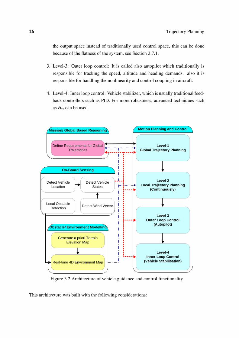
26 Trajectory Planning
the output space instead of traditionally used control space, this can be donebecause of the flatness of the system, see Section 3.7.1.
3. Level-3: Outer loop control: It is called also autopilot which traditionally isresponsible for tracking the speed, altitude and heading demands. also it isresponsible for handling the nonlinearity and control coupling in aircraft.
4. Level-4: Inner loop control: Vehicle stabilizer, which is usually traditional feed-back controllers such as PID. For more robustness, advanced techniques suchas H∞ can be used.
Define Requirements for Global
Trajectories
Mission/ Global Based Reasoning
On-Board Sensing
Obstacle/ Environment Modelling
Generate a priori Terrain
Elevation Map
Real-time 4D Environment Map
Motion Planning and Control
Level-1
Global Trajectory Planning
Detect Vehicle
Location
Detect Vehicle
States
Local Obstacle
DetectionDetect Wind Vector
Level-2
Local Trajectory Planning
(Continuously)
Level-3
Outer Loop Control
(Autopilot)
Level-4
Inner-Loop Control
(Vehicle Stabilisation)
Figure 3.2 Architecture of vehicle guidance and control functionality
This architecture was built with the following considerations:

3.4 Local Trajectory Description 27
• Motion planning has been divided into global and local layers. Therefore, en routeobstacles can be avoided without re-designing the global trajectory. This will reducethe computational time for the whole algorithm.
• Vehicle performance interface between outer-loop control (level-3) and local motionplanning (level-2), so the lower level layer provides vehicle performance specifica-tions to upper level layer (level-2). This will allow local motion planning to be de-signed in the output space rather than the control space, thus the complexity of theproblem will be reduced significantly [56].
• Obstacle sensing and environment modelling were separated from motion planningand control. This also reduces the complexity of design.
• A priori obstacle map is assumed to be available, therefore, the real-time mappingwill just consider the unknown obstacles.
3.4 Local Trajectory Description
There are two most common methods to represent a curve [61]:
1. Implicit equation:f (x,y) = 0 (3.4)
where f is a function of the variables x and y. This equation describes an implicitrelationship between the x and y coordinates of the point lying on the curve.
2. Parametric form: each of the coordinates of a point on the curve is represented sepa-rately as an explicit function of an independent parameter:
P(τ) = (x(τ),y(τ));a <= τ <= b (3.5)
Thus, P(τ): is a vector-valued function of the independent variable τ . Although theinterval [a,b] is arbitrary, it is usually normalized to [0,1]. For example, the firstquadrant of the circle is defined by the parametric functions:
x(τ) = cos(τ)
y(τ) = sin(τ)

28 Trajectory Planning
where 0 ≤ τ ≤ π
2 .Setting u = tan( τ
2)
x(u) =(1−u2)
(1+u2)
y(u) =2u
(1+u2)
where 0 ≤ u ≤ 1. Thus, the parametric representation of a curve is not unique.
3.5 B-Spline Curves
Implementing a geometric modelling system need functions which [61]:
• Precisely representing of all the curves that users of the system need;
• Are easily, efficiently, and accurately processed in a computer, in particular:
1. The computation of point and derivatives on the curves is efficient;
2. Numerically insensitive to the rounding error of floating point;
3. Little memory for storage requirements.
• Are simple and mathematically well understood.
However, single polynomial curves are often inadequate because [62]:
1. A large number of constraints need a polynomial with high degree;
2. Complex shapes require a high degree polynomial to be accurately represented;
The solution is to use curves which are piecewise polynomial, or piecewise rational. Forexample Figure 3.3 shows a curve P(τ) consisting of (m = 5) segments of quadratic poly-nomial. P(τ) is defined on τ ∈ [0,1]. the polynomial segments are joined at τ0 = 0 < τ1 <
τ2 < τ3 < τ4 < τ5 = 1 which called breakpoints,or knots which map into the end point ofeach segments as shown in Figure 3.3. The segments are denoted by Pi(τ),1 ≤ i ≤ m. Thecurve is constructed by joining the segments with some level of continuity. Assume P( j)
i isthe jth derivative of Pi, P(τ) is said to be Pk continuous at breakpoint τi if P( j)
i (τi) = P( j)i+1(τi)
for all 0 ≤ j ≤ k.

3.5 B-Spline Curves 29
1 2 3 4 5 6 70
0.5
1
1.5
2
2.5
x
y
Control polygon
Curve
Control points
Curve Value at the Knots
Figure 3.3 Five segments of quadratic polynomials that join at breakpoints
This thesis uses NURBS curves to describe the trajectory profiles. A NURBS curve isa vector-valued piecewise rational polynomial function. The pth degree NURBS curve isgiven by:
P(τ) =
n
∑i=0
wiNi,p(τ)Ci
n
∑i=0
wiNi,p(τ)
; a ≤ τ ≤ b (3.6)
where wi are the weights, Ci are the control points, and Ni,p(τ) are the pth degree B-splinebasis functions. There are many ways to represent B-spline basis functions. For computerimplementation the recursive representation of B-spline basis functions is the most usefulform [62]. Let U = [u0,u1, ...,um−1,um] be a nondecreasing sequence of real numbers i.e,ui ≤ ui+1, i = 0,1, ...,m− 1, ui called knots or breakpoints, and U is the knot vector thatcontain m+ 1 knots. So the ith B-spline basis function of p-degree (order p+ 1), denotedby Np,i(τ) is defined as:
Ni,0(τ) =
1 if ui ≤ τ < ui+1
0 otherwise
Ni,p(τ) =τ −ui
ui+p −uiNi,p−1(τ)+
ui+p+1 − τ
ui+p+1 −ui+1Ni+1,p−1(τ) (3.7)

30 Trajectory Planning
And Ni,p(τ) = 0 if τ is outside [ui,ui+p+1[ The degree of the basis function p, number ofcontrol point (n+1), and number of the knots (m+1) are related by: m = n+ p+1.
3.5.1 Knot Vector
The knot vector can be realized in different forms, but it must be a nondecreasing sequenceof real numbers (i.e, ui ≤ ui+1, i = 0,1, ...,m−1). Equation (3.7) shows that the knot vectorhas a significant effect on the B-spline basis functions and hence on the resulting B-splinecurve. There are two types of knot vector, periodic and open, in two flavours, uniform andnonuniform [61]. In a uniform knot vector, individual knot values are evenly spaced. Forexample:
U = [ 0 1 2 3 4 5 ]
U = [ −0.3 −0.2 0.1 0 0.1 0.2 0.3 ]
In practice, uniform knot vectors generally begin at zero and are incremented by 1 to somemaximum value, or it can be normalized in range between 0 and 1. A periodic uniform knotvectors will give periodic uniform basis functions for which:
Ni,p(τ) = Ni−1,p(τ −1) = Ni+1,p(τ +1)
Thus, each basis function is a translation of the other.In open uniform knot vector the end knot values has multiplicity equal to the order of theB-spline basis function p+1. For example,
p = 1; U = [ 0 0 1 2 3 4 4 ]
p = 2; U = [ 0 0 0 0 1 2 2 2 2 ]
p = p; U = [ 0 . . 0 up+1 .. um−p−1 1 .. 1 ]( normalized form)
Figure 3.4 shows B-spline basis functions that result by using open uniform knot vector:
U = [ 0 0 0 0.2 0.4 0.6 0.8 1 1 1 ]
The resulting open uniform basis functions yield curves that behave most nearly like Beziercurves. Section 3.6 gives more details about Bezier curve.

3.5 B-Spline Curves 31
0 0.2 0.4 0.6 0.8 10
0.2
0.4
0.6
0.8
1
N(
) i,p
U=[0 0 0 0.2 0.4 0.6 0.8 1 1 1]
Figure 3.4 B-spline basis function p=2 with open uniform knot vector
Nonuniform knot vectors may have either unequally spaced and/or multiple internal knotvalues. They may be periodic or open. This research focus on the open/nonperiodic, andnonuniform knot vector which has the general form:
U = [a, . . . ,a,up+1, . . . ,um−p−1,b, . . . ,b] (3.8)
where the first and end knot has a p+1 multiplicity. Hence for the normalized knot vectora = 0, b = 1.
3.5.2 B-spline Curves Properties
The curve that is given by (3.6) can be written in equivalent form:
P(τ) =n
∑i=0
Ri,p(τ)Ci (3.9)
Ri,p(τ) =wiNi,p(τ)Cin
∑i=0
wiNi,p(τ)
; a ≤ τ ≤ b(3.10)
where Ri,p(τ) are rational basis functions. The analytical properties of Ri,p(τ) determinethe geometric behaviour of the curves [62].

32 Trajectory Planning
• Generalization: If wi = 1 then
Ri,p(τ) =
Bi,p(τ) if U = [0,0, . . . ,0,1,1, . . . ,1]
Ni,p(τ) otherwise(3.11)
where the zeros and ones in U are repeated with multiplicity p+ 1, and Bi,p is theBernstein polynomial of degree p, which are the basis of Bezeir curve.
• If n = p and U = [0, . . . ,0,1, . . . ,1] then P(τ) is a Bezier curve.
• End point interpolation: P(0) =C0 and P(1) =Cn.
• Strong convex hull property: the curve is contained in the convex hull of its controlpolygon. If τ ∈ [ui,ui+1[, p≤ i<m− p−1, then P(τ) is in the convex hull of controlpoints Ci−p, . . . ,Ci. Figure 3.5 shows quadratic (p= 2) B-spline curve and its B-splinebasis functions. The control points are:
C = {(1,1),(0.5,2),(4,2),(3,1),(2,0),(4.5,0.2)} (3.12)
and the knot vector is
U = [0,0,0,0.25,0.5,0.75,1,1,1] (3.13)
It can be seen that the part of the curve that results from τ ∈ [τ3,τ4[= [0.25,0.5[ iscontained in the convex hull which is created by control points C2,C3,C4. Due to thestrong convex hull property it can be seen in Figure 3.5 the straight line that exists inthe duration τ ∈ [τ4,τ5[= [0.5,0.75[ is due to the co-linear control points C3,C4,C5.
• Portion of unity: ∑i Ri,p(τ) = 1
• Differentiability: The rational basis functions are infinity continuously differentiablein the interior of a knot span [61]. But at a knot they are p− k times continuouslydifferentiable where k is the multiplicity of the knot. Due to this property cusps canoccur. Figure 3.6 shows a quadratic curve p = 2 that is generated by using knot vectorU = [0,0,0, 1
5 ,25 ,
35 ,
45 ,
45 ,1,1,1] it can be seen that the cusp occurs because the knot at
45 has multiplicity k = 2 so the curve is p− k = 0 continuously differentiable at thisknot.

3.5 B-Spline Curves 33
0 0.5 1 1.5 2 2.5 3 3.5 4 4.5 5
0
0.5
1
1.5
2
x
y
0 0.1 0.2 0.3 0.4 0.5 0.6 0.7 0.8 0.9 10
0.2
0.4
0.6
0.8
1
Ni,p
()
B-spline Basis Functions
U=[0 0 0 0.25 0.5 0.75 1 1 1]
Control polygon
Curve
Control point
Curve at the Knots
Figure 3.5 Convex hull property of B-spline curve
1 1.5 2 2.5 3 3.5 4 4.5 5 5.51
1.5
2
2.5
3
3.5
4
x
y
0 0.1 0.2 0.3 0.4 0.5 0.6 0.7 0.8 0.9 10
0.2
0.4
0.6
0.8
1
N(
) i,p
B-spline Basis FunctionsU=[0 0 0 0.2 0.4 0.6 0.8 0.8 1 1 1]
Control polygon
Curve
Control point
Curve value at the Knots
Figure 3.6 A quadratic curve p = 2 with cusp

34 Trajectory Planning
It worth mentioning that the continuity can be recovered by control point modification.For example, by reallocating the control point C6 to be co-linear with C4 and C5 asshown in Figure 3.7.
• Figure 3.7 shows that the moving of C6 only modifies the curve in the interval [τ6,τ9[
this property is called local modification scheme. Generally speaking, moving Ci willchange the B-spline curve P(τ) only in the interval [τi,τi+p+1[.
• The control polygon which formed by the control point is a linear approximation tothe curve.
1 1.5 2 2.5 3 3.5 4 4.5 5 5.51
1.5
2
2.5
3
3.5
4
x
y
0 0.1 0.2 0.3 0.4 0.5 0.6 0.7 0.8 0.9 10
0.2
0.4
0.6
0.8
1
N(
) i,p
B-spline Basis FunctionsU=[0 0 0 0.2 0.4 0.6 0.8 0.8 1 1 1]
Control polygon
Curve
Control point
Curve value at the Knots
Figure 3.7 Cusp removing by reallocating the control point
3.5.3 Derivatives of B-Spline Curves
The derivatives of B-spline curves can be calculated simply by computing the derivatives oftheir B-spline basis functions. P(k)(τ) which is the kth derivative of P(τ) is given by:
P(k)(τ) =n
∑i=0
N(k)i,p (τ)Ci (3.14)
3.6 Bezier Curve 35
where N(k)i,p (τ) is the kth derivative of B-spline basis functions which can be calculated re-
cursively:
N(k)i,p (τ) =
N(k−1)i,p−1 (τ)
ui+p −ui−
N(k−1)i+1,p−1(τ)
ui+p+1 −ui+1
p (3.15)
The first derivative of B-spline basis function is:
N(1)i,p (τ) =
pui+p −ui
Ni,p−1(τ)−p
ui+p+1 −ui+1Ni+1,p−1(τ) (3.16)
3.6 Bezier Curve
Bezier curves are special case of NURBS when the all wights equal to unity wi = 1 and theknot vector takes the following form: U = [0,0, . . . ,0,1,1, . . . ,1]
P(τ) =n
∑i=0
Bi(τ)Ci (3.17)
where P(τ) is the Bezier curve, n is the order of the polynomial, τ is the curve parameter,Bi(τ) is the ith order basis function that can be calculated by (3.11), and Ci are the coeffi-cients (control points) of ith basis function.A 6th order Bezier curves are used to describe the local trajectory profiles in this thesis.Using Bezeir curves to describe local trajectories will reduce the overall dimension of theproblem [10] (the optimisation problem will be to find the control points (Ci), which alsocalled the polynomial coefficients). Sixth order curves were used in [10] for local motionplanning for a small quad-rotor UAV as they are considered to provide a good compromisebetween dynamic flexibility over the design horizon and number of design variables. Thesmall quad-rotor UAV has more maneuverability than the fixed wing UAV ( a fixed wingUAV dose not have the ability to fly backward and hovering like a quad-rotor UAV). How-ever, one can consider a lower order of Bezeir curve but the order must not be lower than 4as these curves are differentiated to calculate speed, acceleration, and the rate of accelera-tion. Study the effect of using different order of the polynomial on the trajectory planningalgorithm is out of the scope of this thesis and it can be curried out as a future work.The basis functions that generate the Bezier curves are known as Bernstein polynomials andthey are calculated by using (3.7-3.11), thus, for example, the 6th order Bezier curve basis

36 Trajectory Planning
functions are:
B0 = (1− τ)6
B1 = 6τ(1− τ)5
B2 = 15τ2(1− τ)4
B3 = 20τ3(1− τ)3 (3.18)
B4 = 15τ4(1− τ)2
B5 = 6τ5(1− τ)
B6 = τ6
Figure 3.8 shows Bezier curve (p = 6), and its basis functions (Bernstein basis function), itcan be noticed that the first basis function which is B0 has significant effect on the start pointof the curve, while B6 controls the end point of the curve and the rest of the basis functionshave no effect on the start and the end points. This is one of advantages of the Bezier curve,this property will reduce the computational time during trajectory optimisation. Substitut-ing (3.18) in (3.17) gives a 6th order polynomial (Bezier curve), after deciding the orderof the polynomial that is going to be used in generating the local trajectory, the trajectoryshape will vary with coefficients Ci (control points). The Bezier curve shaping in Figure 3.8is generated by using C = {(1,2),(2,3),(3,2),(4,4),(5,4),(6,0),(7,3)} as control points.
1 2 3 4 5 6 70
1
2
3
4
x
y
0 0.1 0.2 0.3 0.4 0.5 0.6 0.7 0.8 0.9 10
0.2
0.4
0.6
0.8
1
N(
) i,p
Bernstein basis functionsU=[0 0 0 0 0 0 0 1 1 1 1 1 1 1]
Control polygon
Curve
Control point
Curve value at the Knots
B0
B1
B2
B3
B4
B5
B6
Figure 3.8 Bezier curve(upper), and its basis functions (lower)

3.6 Bezier Curve 37
3.6.1 Trajectory Profiles Description Using Polynomial Functions
As mentioned earlier using the polynomial functions to describe the trajectory profiles (i.e.positions, velocities, accelerations, and jerks) reduces the computational time for trajectoryoptimisation. The speed profiles in forward (u), lateral (v), and vertical (w) axes can bewritten by using polynomial functions (6th order Bezier function):
u(τ) = cu0B0(τ)+ cu
1B1(τ)+ cu2B2(τ)+ · · ·+ cu
6B6(τ)
v(τ) = cv0B0(τ)+ cv
1B1(τ)+ cv2B2(τ)+ · · ·+ cv
6B6(τ) (3.19)
w(τ) = cw0 B0(τ)+ cw
1 B1(τ)+ cw2 B2(τ)+ · · ·+ cw
6 B6(τ)
Using sixth order polynomial functions to describe the speed profiles gives a good flexibil-ity over the design horizon with an acceptable number of design variables (the polynomialcoefficients) [56]. Calculation of acceleration, jerk, and position profiles can be done by tak-ing the first derivative of (3.19) for the acceleration profiles, the second derivative of (3.19)for the jerk profiles, and integration of (3.19) for the position profiles. In order to do so, arelationship between the curve parameter τ and the time t must be defined. A fixed timehorizon (th) was used so t can be represented by:
t = th.τ (3.20)
hence the acceleration profiles can be calculated:
dudt
=dudτ
· dτ
dt=
1th· du
dτ⇒ (3.21)
u(τ) =1th
(cu
0dB0(τ)
dτ+ cu
1dB1(τ)
dτ+ cu
2dB2(τ)
dτ+ · · ·+ cu
6dB6(τ)
dτ
)(3.22)
andd2udt2 =
1t2h· d2u
dτ2 (3.23)
hence
u(τ) =1t2h
(cu
0d2B0(τ)
dτ2 + cu1
d2B1(τ)
dτ2 + cu2
d2B2(τ)
dτ2 + · · ·+ cu6
d2B6(τ)
dτ2
)(3.24)
The acceleration and jerk profiles for the lateral and vertical axis can be calculated in asimilar way. The position profiles are calculated by integrating the basis functions with
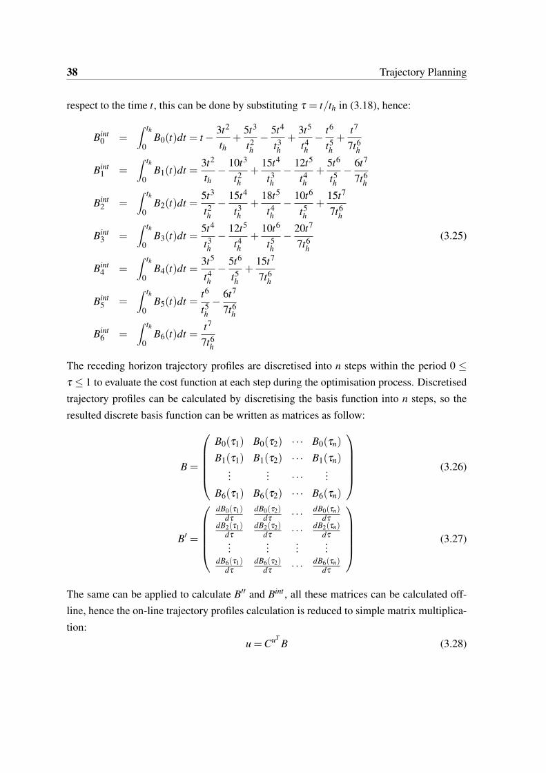
38 Trajectory Planning
respect to the time t, this can be done by substituting τ = t/th in (3.18), hence:
Bint0 =
∫ th
0B0(t)dt = t − 3t2
th+
5t3
t2h− 5t4
t3h+
3t5
t4h− t6
t5h+
t7
7t6h
Bint1 =
∫ th
0B1(t)dt =
3t2
th− 10t3
t2h
+15t4
t3h
− 12t5
t4h
+5t6
t5h− 6t7
7t6h
Bint2 =
∫ th
0B2(t)dt =
5t3
t2h− 15t4
t3h
+18t5
t4h
− 10t6
t5h
+15t7
7t6h
Bint3 =
∫ th
0B3(t)dt =
5t4
t3h− 12t5
t4h
+10t6
t5h
− 20t7
7t6h
(3.25)
Bint4 =
∫ th
0B4(t)dt =
3t5
t4h− 5t6
t5h+
15t7
7t6h
Bint5 =
∫ th
0B5(t)dt =
t6
t5h− 6t7
7t6h
Bint6 =
∫ th
0B6(t)dt =
t7
7t6h
The receding horizon trajectory profiles are discretised into n steps within the period 0 ≤τ ≤ 1 to evaluate the cost function at each step during the optimisation process. Discretisedtrajectory profiles can be calculated by discretising the basis function into n steps, so theresulted discrete basis function can be written as matrices as follow:
B =
B0(τ1) B0(τ2) · · · B0(τn)
B1(τ1) B1(τ2) · · · B1(τn)...
... · · · ...B6(τ1) B6(τ2) · · · B6(τn)
(3.26)
B′ =
dB0(τ1)
dτ
dB0(τ2)dτ
· · · dB0(τn)dτ
dB2(τ1)dτ
dB2(τ2)dτ
· · · dB2(τn)dτ
......
......
dB6(τ1)dτ
dB6(τ2)dτ
· · · dB6(τn)dτ
(3.27)
The same can be applied to calculate B′′ and Bint , all these matrices can be calculated off-line, hence the on-line trajectory profiles calculation is reduced to simple matrix multiplica-tion:
u =CuTB (3.28)

3.6 Bezier Curve 39
u =1th
CuTB′ (3.29)
u =1t2h
CuTB′′ (3.30)
x = x0 +CuTBint (3.31)
where CuTis the vector of coefficients for forward axis:
CuT=[
cu0 cu
1 · · · cu6
](3.32)
The trajectory profiles for lateral and vertical axis can be calculated in a similar way. Theoptimisation problem is to find the polynomial coefficients, till now there are twenty-onecoefficients that have to be calculated (seven coefficients for each axes).
3.6.2 Boundary Conditions
Aircraft states can be measured by the sensing unit, the current states can be used as bound-ary conditions that guarantee a smooth transition from current states to target states. Substi-tuting τ = 0 in trajectory profiles (3.19), (3.21), and (3.23) gives:
cu0 = u0
cu1 =
th6
u0 + cu0 (3.33)
cu2 =
t2h
30u0 − cu
0 +2cu1
where:u0: is the initial forward speed,u0: is the initial forward acceleration,u0: is the initial forward jerk.Similarly for the lateral and vertical trajectory profiles, the first three coefficients can befound, so the number of design variables has been reduced from twenty-one into twelvevariables.
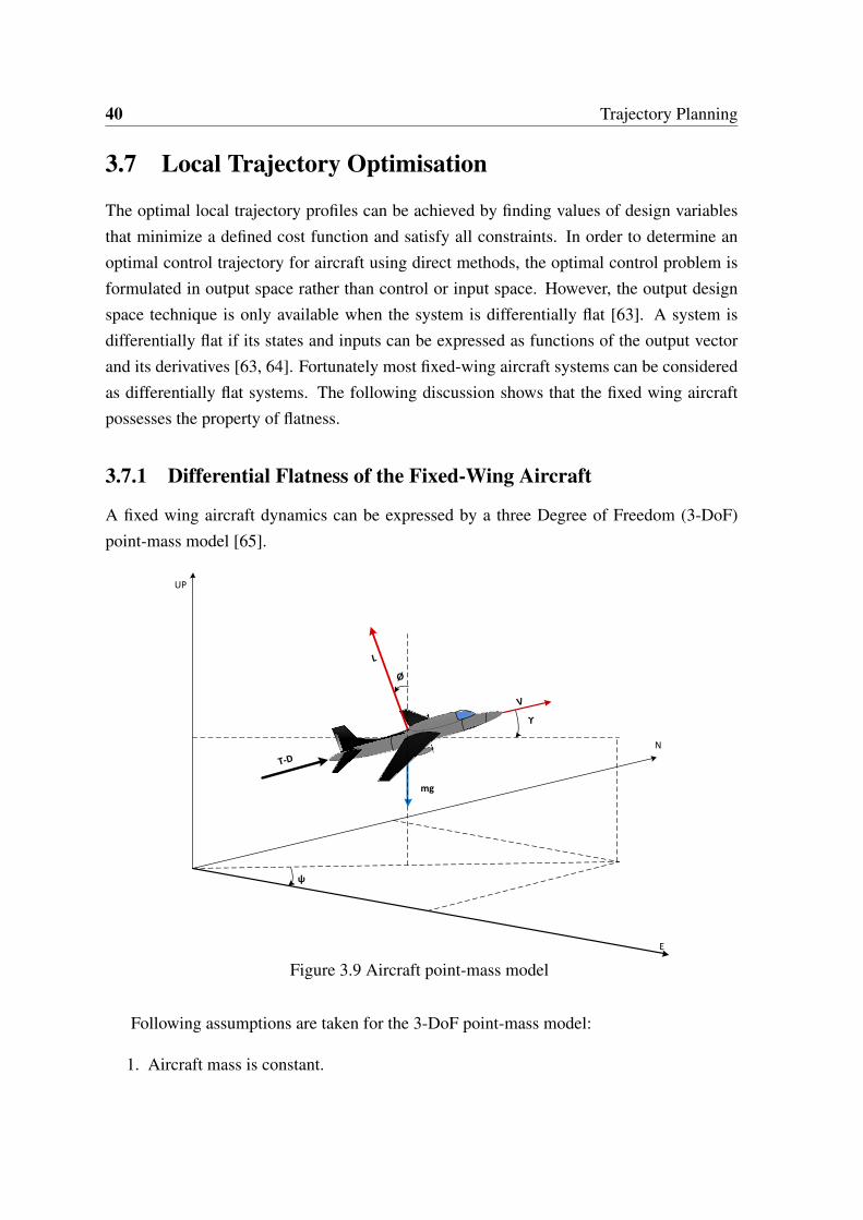
40 Trajectory Planning
3.7 Local Trajectory Optimisation
The optimal local trajectory profiles can be achieved by finding values of design variablesthat minimize a defined cost function and satisfy all constraints. In order to determine anoptimal control trajectory for aircraft using direct methods, the optimal control problem isformulated in output space rather than control or input space. However, the output designspace technique is only available when the system is differentially flat [63]. A system isdifferentially flat if its states and inputs can be expressed as functions of the output vectorand its derivatives [63, 64]. Fortunately most fixed-wing aircraft systems can be consideredas differentially flat systems. The following discussion shows that the fixed wing aircraftpossesses the property of flatness.
3.7.1 Differential Flatness of the Fixed-Wing Aircraft
A fixed wing aircraft dynamics can be expressed by a three Degree of Freedom (3-DoF)point-mass model [65].
N
E
UP
ψ
V
T-D
L
mg
ϒ
Ø
Figure 3.9 Aircraft point-mass model
Following assumptions are taken for the 3-DoF point-mass model:
1. Aircraft mass is constant.
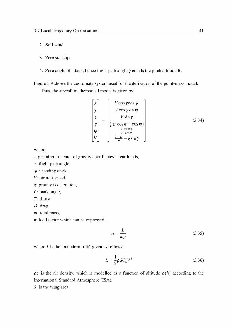
3.7 Local Trajectory Optimisation 41
2. Still wind.
3. Zero sideslip
4. Zero angle of attack, hence flight path angle γ equals the pitch attitude θ .
Figure 3.9 shows the coordinate system used for the derivation of the point-mass model.
Thus, the aircraft mathematical model is given by:
x
y
z
γ
ψ
V
=
V cosγ cosψ
V cosγ sinψ
V sinγ
gV (ncosφ − cosψ)
gV
nsinφ
cosγ
T−Dm −gsinγ
(3.34)
where:x,y,z: aircraft center of gravity coordinates in earth axis,γ: flight path angle,ψ : heading angle,V : aircraft speed,g: gravity acceleration,φ : bank angle,T : thrust,D: drag,m: total mass,n: load factor which can be expressed :
n =L
mg(3.35)
where L is the total aircraft lift given as follows:
L =12
ρSCLV 2 (3.36)
ρ: is the air density, which is modelled as a function of altitude ρ(h) according to theInternational Standard Atmosphere (ISA).S: is the wing area.
42 Trajectory Planning
CL: is the lift coefficient given by:
CL =CL0 +αCLα(3.37)
where CL0 , CLαare the zero-angle-of-attack lift coefficient, lift curve slope.
The total aerodynamic drag D is given by [66]:
D =12
ρSCDV 2 (3.38)
where CD is the drag coefficient given by:
CD =CD0 + kC2L (3.39)
where CD0 and k are the minimum drag coefficient and induced drag factor respectively.The output vector can be expressed by:
Y =
x
y
z
(3.40)
The input vector can be taken as:
U =
φ
T
n
(3.41)
By modifying (3.34) one can find:
V =√
x2 + y2 + z2 (3.42)
γ = arcsin(zV) (3.43)
ψ = arcsin(y
V cosγ) (3.44)
φ = arctan(ψV cosγ
gcosγ +V ˙γ) (3.45)

3.7 Local Trajectory Optimisation 43
n =gcosγ +V γ
gcosφ(3.46)
T = D+mV +mgsinγ (3.47)
It can be noticed from (3.42-3.38) that the controls and the states of the system canbe expressed as functions of the output vector and its derivatives. Hence the system isdifferentially flat. So the optimal control problem can be formulated in the output spacerather than the control space.The aircraft and the obstacles constraints are augmented in the cost function by using apenalty function method.
3.7.2 Aircraft Constraints
Penalty functions are used to ensure that the resulting optimal trajectory will be achievedwithout exceeding the aircraft performance limits. Hence, the cost function is augmentedwith additional terms that prevent the solution approaching the limits. The Yukawa potentialfunction is used in this thesis:
Cp = Ape−αpdp
dp(3.48)
where:Cp: aircraft performance constraint term to be added to the total cost function,Ap: scaling factor,αp: decay rate,dp: performance margin given by:
dp = 1−1(
current state valuestate maximum \ minimum value
)(3.49)
To avoid zero value of dp a minimum performance margin value dmin must be defined so:if dp ≤ dmin then dp = dmin. The role of the penalty function can be understood from Fig-ure 3.10 which shows the value of the potential function with respect to the value of theperformance margin at different values of scaling factor Ap. It can be clearly seen that whenthe performance margin decreases (which means that when the current state value is close toits limit) the potential function takes a huge value. Thus the total cost function will increasesignificantly, so the optimisation algorithm will try to find another solution that keeps theaircraft state away from its limits.
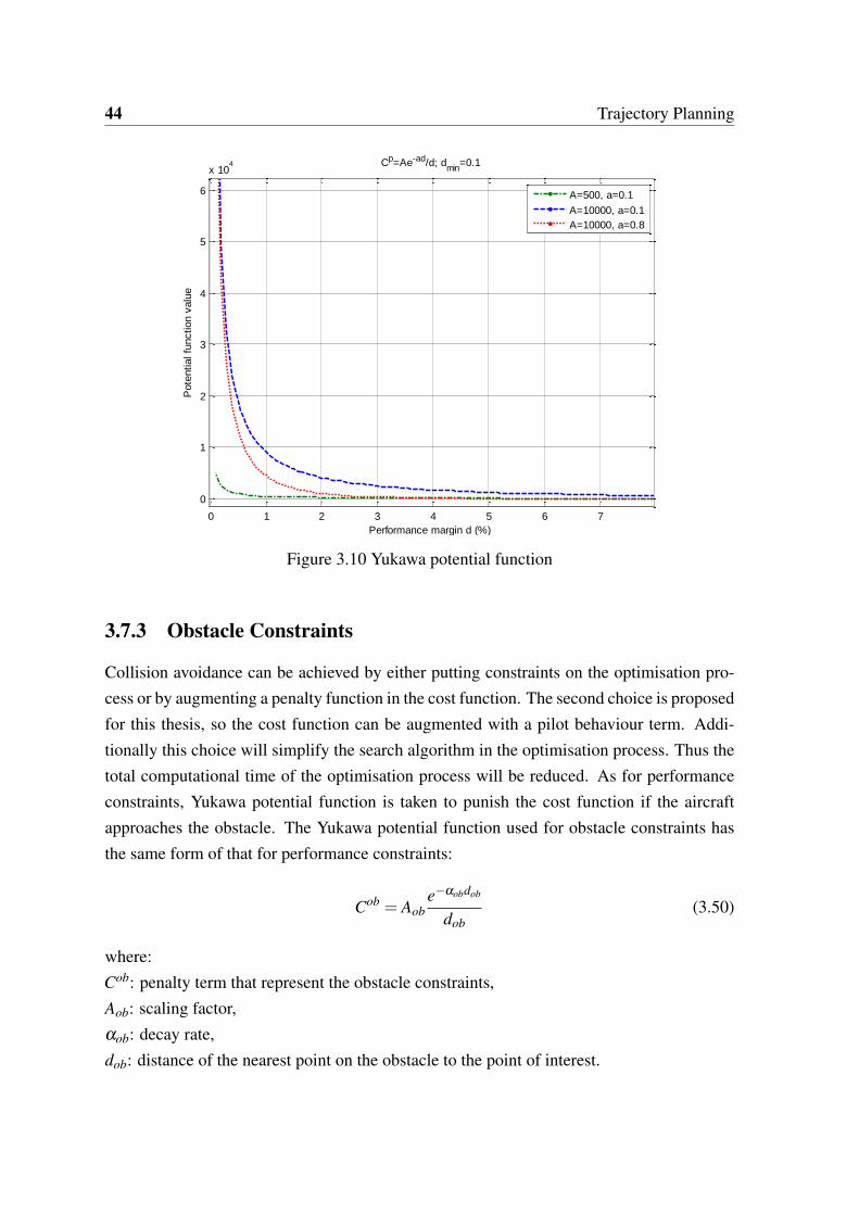
44 Trajectory Planning
0 1 2 3 4 5 6 7
0
1
2
3
4
5
6
x 104
Performance margin d (%)
Pote
ntial fu
nction v
alu
e
Cp=Ae-ad/d; dmin
=0.1
A=500, a=0.1
A=10000, a=0.1
A=10000, a=0.8
Figure 3.10 Yukawa potential function
3.7.3 Obstacle Constraints
Collision avoidance can be achieved by either putting constraints on the optimisation pro-cess or by augmenting a penalty function in the cost function. The second choice is proposedfor this thesis, so the cost function can be augmented with a pilot behaviour term. Addi-tionally this choice will simplify the search algorithm in the optimisation process. Thus thetotal computational time of the optimisation process will be reduced. As for performanceconstraints, Yukawa potential function is taken to punish the cost function if the aircraftapproaches the obstacle. The Yukawa potential function used for obstacle constraints hasthe same form of that for performance constraints:
Cob = Aobe−αobdob
dob(3.50)
where:Cob: penalty term that represent the obstacle constraints,Aob: scaling factor,αob: decay rate,dob: distance of the nearest point on the obstacle to the point of interest.

3.7 Local Trajectory Optimisation 45
Although using a potential function to describe the obstacle constraints complicates the costfunction, it simplifies the search algorithm. Another advantage of using potential functionis that it handles the collision event in a manner which is close to human behaviour. Forexample, an avoidance manoeuvre can vary according to many factors such as aircraft speed,obstacle speed, aircraft manoeuvrability, and obstacle manoeuvrability. Additionally, due tothe difficulty in generating a full 3D illustration for the obstacles that can be detected by anon-board sensor unit (this description is very important to add constraints to the optimisationprocess) the potential function approach does not need a 3D description of the obstacle.It just needs the distance between the aircraft and the nearest point in the obstacle [56].However, Becerra [67] has shown that ill conditioning and difficulty in choosing a suitablevalue for the penalty factor are the main disadvantages of the penalty function approach.
3.7.4 Total Cost Function
The following cost function is used in the optimisation process:
J =n
∑i=1
[λpositionJpositioni +λspeedJspeed
i +λper f ormanceJper f ormancei +λobJob
i ]+λtJt (3.51)
where:
Jpositioni = (xdemand
i − xactuali )2 +(ydemand
i − yactuali )2 +(zdemand
i − zactuali )2 (3.52)
Jspeedi = (udemand
i −uactuali )2 +(vdemand
i − vactuali )2 +(wdemand
i −wactuali )2 (3.53)
Jper f ormance =q
∑j=1
Ape−αpdp
dp(3.54)
Jobi =
m
∑j=1
Aobe−αobdob
dob(3.55)
Jt = λh(ψdemandn −ψ
actualn )2 +(λ f (γ
demandn − γ
actualn )2 (3.56)
λ : scaling factor,n: number of points that will be evaluated across the design horizon,q: number of performance constraints,

46 Trajectory Planning
m: number of detected obstacles,ψ: heading angle,γ: flight path angle,It can be seen that the cost function given by (3.51) makes a balance between the differentterms: trajectory tracking terms (Jposition,Jspeed,Jt); and constraints terms (obstacle avoid-ance term Job, performance constraint term Jper f ormance). This balance can be controlledby changing the scaling factors λ . The scaling factors can be constants or they may varyaccording to the situation. In other words, the priority of the cost function terms can bevaried in order to allow the aircraft to fly safely in different flight scenarios.
3.7.5 Avoiding Local Minima
The performance constraints tend to act as an enclosing boundary around the entire searchspace, hence are less likely to result in local minimum. Thus, the obstacle constraints arethe primary source of the local minima. When obstacles are detected this can have the im-pact of dividing the feasible design space into unconnected regions, therefore, reducing theeffectiveness of the solver of the optimisation problem. The possibility of getting trapped inlocal minimum is reduced by providing a mechanism for the search to jump to the differentregions of the design space. This is achieved by generating a set of candidate trajectoriesthen comparing the cost for each candidate then selecting the one that gives the minimumcost to initiate the optimisation problem solver. The candidate trajectories are generated byapplying maximum/minimum inputs to the vehicle model with the current vehicle states asinitial states to ensure that the maximum performance manoeuvres in each axis are alwaysavailable if required. This method does not guarantee that the chosen initial solution lieswithin the region of the design space that provides the best solution. In this case the inputcommands are:
φ =[
φmin φc φmax
]T =
[Tmin Tc Tmax
](3.57)
n =[
nmin nc nmax
]where φc, Tc, and nc are the current values of the inputs, and φmin/max, Tmin/max, and nmin/max
are the minimum and maximum values of the inputs which can be calculated from thevehicle specifications (the Aerosonde UAV [68] model and specifications are used here).This combination will produce 27 candidate trajectories.

3.8 Simulation Results 47
3.8 Simulation Results
This section demonstrates simulation results of different scenarios. The global trajectorythat was used in all scenarios is level flight with constant speed v = 30m.s−1 at 1000m
altitude, with heading ψ = 0 rad. Still air is assumed. The receding horizon time is th =
20 sec and sampling time ts = 0.2 sec. The optimisation process is updated every 2 sec.The system is built in MATLAB/Simulink and the fminunc function is used as a solverfor the optimisation problem. Scaling factors values are: λposition = 100, λspeed = 500,λper f ormance = 1, λob = 1, λt = 1, λh = 10, λ f = 1.
Inverse
DynamicsAircraft Model
Local Trajectory
Planner
(On-line)
Trajectory
profiles Predefined
Global Trajectory
Vehicle state
Local Obstacles
Detection( states
estimation)
Controllers
Figure 3.11 Block diagram of the proposed CAS
3.8.1 Global Trajectory Tracking with Static Obstacle Avoidance
In this scenario the initial position of the UAV is higher than the global trajectory by 200m,but the UAV is flying at the same speed and direction as the global trajectory. There isalso a static obstacle that the UAV must avoid during the global trajectory tracking process.Figure 3.12 shows the simulation result of this scenario, it can be seen that the UAV isconverging to the global trajectory then when the static obstacle appears in its way, theUAV performs the necessary manoeuvre in order to avoid the obstacle. Then the UAVconverges again to the global trajectory after passing the static obstacle. Figure 3.13 showstime histories of some state variables of the UAV ( position, speed, heading angle ψ , andflight path angle γ) during this scenario.

48 Trajectory Planning
01000
20003000 4000
50006000
-500
0
500
200
400
600
800
1000
1200
1400
X: 3326
Y: 26.46
Z: 1314
X [m]
X: 0
Y: 10
Z: 1200
Y [m]
X: 0
Y: 10
Z: 1000
Z [
m]
Global Trajectory
Static Obsticale
UAV
Local Trajectory
Figure 3.12 Converging to the global trajectory and avoiding a static obstacle
0 50 100 150 2000
5000
10000
x [m
]
0 50 100 150 200-50
0
50
y [m
]
0 50 100 150 200500
1000
1500
z [m
]
Time [sec]
0 50 100 150 20025
30
35
V [m
/se
c]
0 50 100 150 200-0.2
0
0.2
[ra
d]
0 50 100 150 200-0.5
0
0.5
[r
ad
]
Time [sec]
Figure 3.13 Position, speed, ψ , and γ state during the avoidance manoeuvre (static obstacle)
Figure 3.14 gives the normal load factor which is slightly deviating around one andmeets the load criteria (n ∈ [−1,2.5]) given by CS-23 document [69].

3.8 Simulation Results 49
0 20 40 60 80 100 120 140 160 180 2000.85
0.9
0.95
1
1.05
1.1
Time [sec]
Load f
acto
r
Figure 3.14 Load factor during the avoidance manoeuvre
Note that the resulting optimal trajectory is dependent on the chosen scaling factors (orweightings) of the terms in the objective cost of the optimal control problem. Hence the re-sulting solution may be sensitive to the choice of the scaling factors. The issue of selectingthe best weightings for optimal control problems has been explored for fixed gain feedbackcontrollers (for example see [70, 71]). For trajectory optimization problems, it appears lesswell-studied [72], but has been considered for model predictive control [73]. In addition,ill conditioning problems can arise when using penalty functions in the cost function anddifficulties in choosing a suitable value for the penalty factor makes it difficult to tune thescaling factors [67]. In this thesis, trial and error is used for selecting the scaling factors.Figure 3.15 and Figure 3.16 show the same simulation results ,but from different view an-gles, that show the sensitivity of the generated trajectory to the scaling factors values. Theseresults show the effects of scaling factors λ on the UAV avoidance manoeuver that gener-ated to avoid a static obstacle and track a global trajectory. It can be seen that there areobvious differences between the generated avoidance trajectories, not only in the shape ofthe trajectories, but also in the direction of the avoidance manoeuvrers. As it can be seen inFigure 3.15 and Figure 3.16 there are four trajectories each one is generated with differentscaling factors that are given in Table 3.1:
Table 3.1 Scaling factors values
Scaling factor λposition λspeed λper f ormance λob λt
1st avoidance manoeuvre 1 1 1 1 1
2nd avoidance manoeuvre 1 1 1 10 1
3rd avoidance manoeuvre 100 1 10 1 1
4th avoidance manoeuvre 10 1 1 1 1

50 Trajectory Planning
0 500 1000 1500 2000 2500 3000-500
0
500
500
600
700
800
900
1000
1100
1200
1300
1400
1500
UAV initial position
Global trajectory
Obstacle
1st Manoeuvre
2nd Manoeuvre
3rd Manoeuvre
4th Manoeuvre
Z [m
]
Y [m]
X [m]
Figure 3.15 Scaling factors effects on the generated trajectory (view 1)
-500-400-300-200-1000100200300400500
500
600
700
800
900
1000
1100
1200
1300
1400
1500
UAV initial position
Global trajectory
Obstacle
1st Manoeuvre
2nd Manoeuvre
3rd Manoeuvre
4th Manoeuvre
Z [m
]
Y [m]
Figure 3.16 Scaling factors effects on the generated trajectory (view 2)
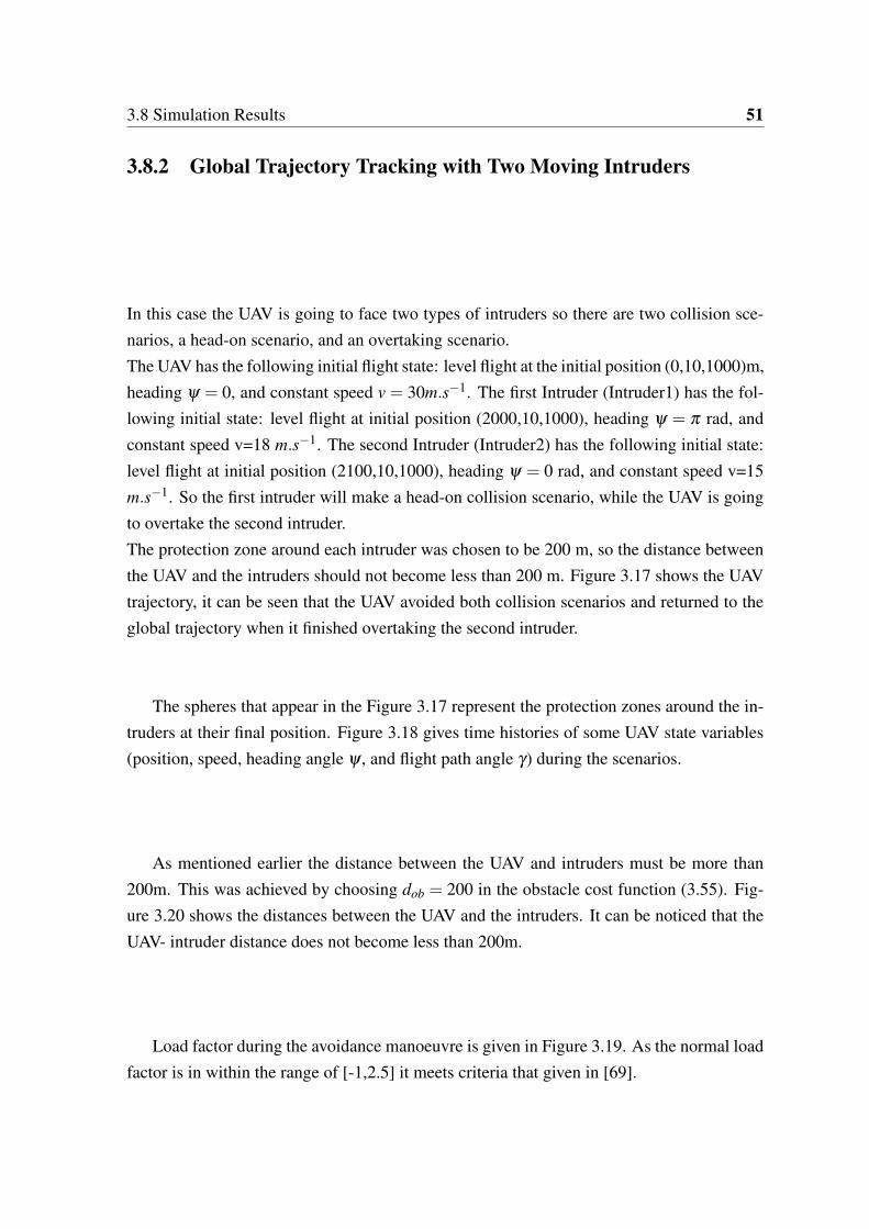
3.8 Simulation Results 51
3.8.2 Global Trajectory Tracking with Two Moving Intruders
In this case the UAV is going to face two types of intruders so there are two collision sce-narios, a head-on scenario, and an overtaking scenario.The UAV has the following initial flight state: level flight at the initial position (0,10,1000)m,heading ψ = 0, and constant speed v = 30m.s−1. The first Intruder (Intruder1) has the fol-lowing initial state: level flight at initial position (2000,10,1000), heading ψ = π rad, andconstant speed v=18 m.s−1. The second Intruder (Intruder2) has the following initial state:level flight at initial position (2100,10,1000), heading ψ = 0 rad, and constant speed v=15m.s−1. So the first intruder will make a head-on collision scenario, while the UAV is goingto overtake the second intruder.The protection zone around each intruder was chosen to be 200 m, so the distance betweenthe UAV and the intruders should not become less than 200 m. Figure 3.17 shows the UAVtrajectory, it can be seen that the UAV avoided both collision scenarios and returned to theglobal trajectory when it finished overtaking the second intruder.
The spheres that appear in the Figure 3.17 represent the protection zones around the in-truders at their final position. Figure 3.18 gives time histories of some UAV state variables(position, speed, heading angle ψ , and flight path angle γ) during the scenarios.
As mentioned earlier the distance between the UAV and intruders must be more than200m. This was achieved by choosing dob = 200 in the obstacle cost function (3.55). Fig-ure 3.20 shows the distances between the UAV and the intruders. It can be noticed that theUAV- intruder distance does not become less than 200m.
Load factor during the avoidance manoeuvre is given in Figure 3.19. As the normal loadfactor is in within the range of [-1,2.5] it meets criteria that given in [69].
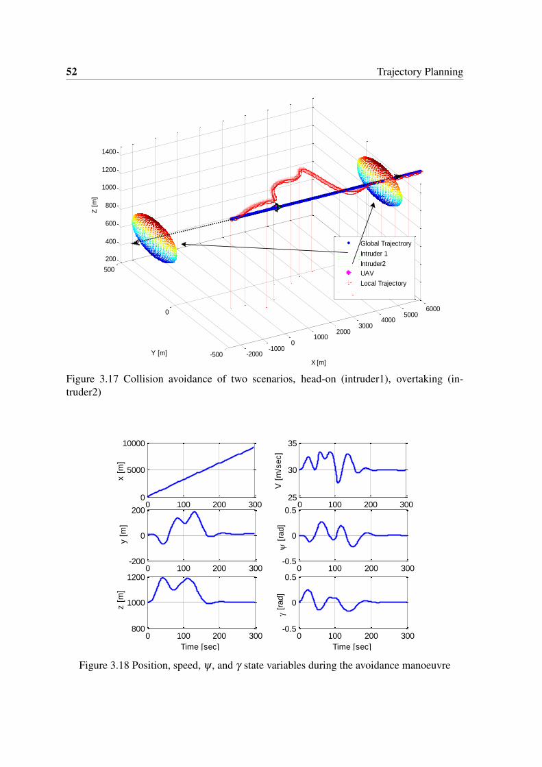
52 Trajectory Planning
-2000-1000
01000
20003000
40005000
6000
-500
0
500
200
400
600
800
1000
1200
1400
X [m]
Y [m]
Z [
m]
Global Trajectrory
Intruder 1
Intruder2
UAV
Local Trajectory
Figure 3.17 Collision avoidance of two scenarios, head-on (intruder1), overtaking (in-truder2)
0 100 200 3000
5000
10000
x [
m]
0 100 200 300-200
0
200
y [
m]
0 100 200 300800
1000
1200
z [
m]
Time [sec]
0 100 200 30025
30
35
V [
m/s
ec]
0 100 200 300-0.5
0
0.5
[
rad]
0 100 200 300-0.5
0
0.5
[r
ad]
Time [sec]
Figure 3.18 Position, speed, ψ , and γ state variables during the avoidance manoeuvre
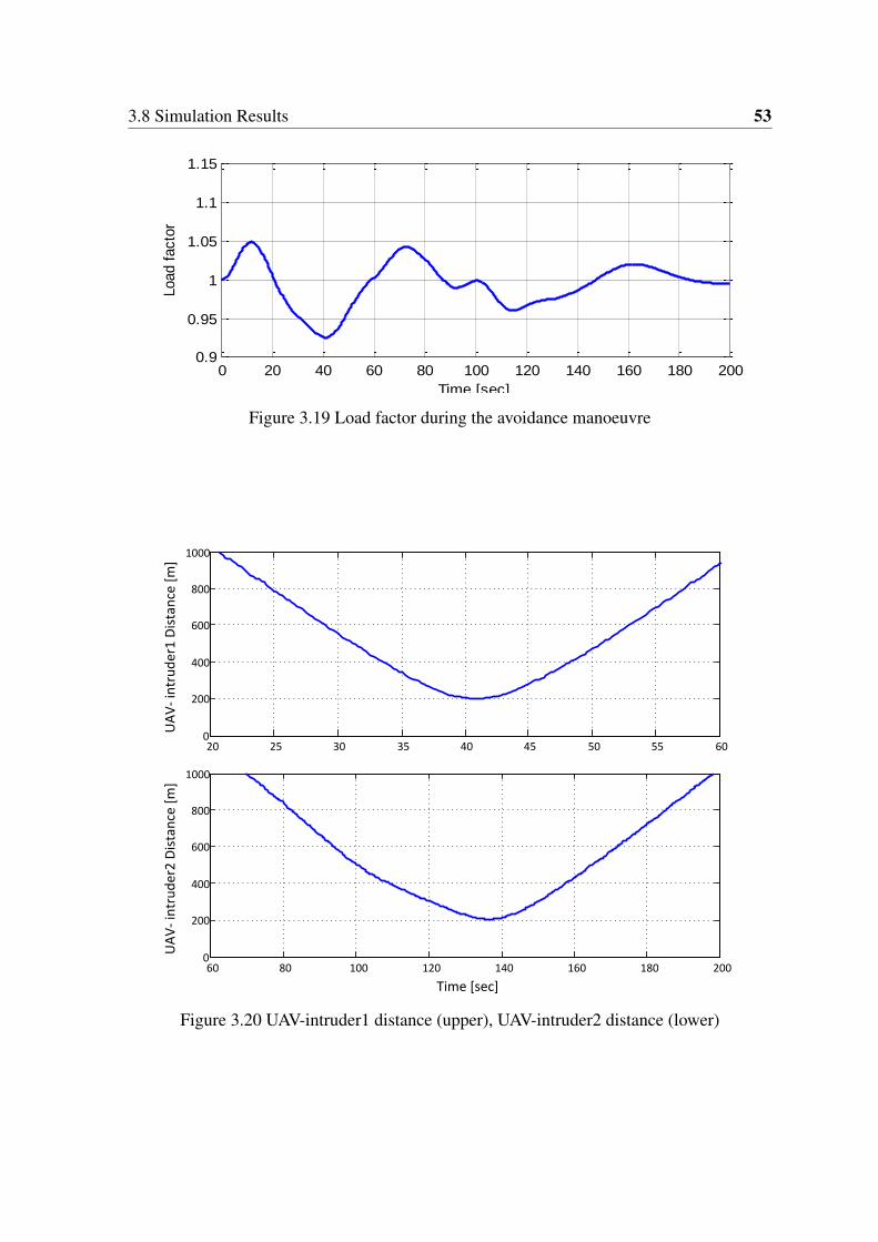
3.8 Simulation Results 53
0 20 40 60 80 100 120 140 160 180 2000.9
0.95
1
1.05
1.1
1.15
Time [sec]
Load f
acto
r
Figure 3.19 Load factor during the avoidance manoeuvre
20 25 30 35 40 45 50 55 600
200
400
600
800
1000
UA
V-
intr
ud
er1
Dis
tan
ce [
m]
60 80 100 120 140 160 180 2000
200
400
600
800
1000
Time [sec]
UA
V-
intr
ud
er2
Dis
tan
ce [
m]
Figure 3.20 UAV-intruder1 distance (upper), UAV-intruder2 distance (lower)

54 Trajectory Planning
3.9 Summary
This chapter presents a local trajectory planning algorithm that is used for the collisionavoidance system for a fixed-wing aircraft. A real-time collision avoidance algorithm isdeveloped based on parameterizing an optimal control problem with B-spline curves. Theoptimal control problem is formulated in output space rather than control or input space,which is feasible because of the differential flatness of the system for a fixed wing aircraft.The flat output trajectory is parameterized using a B-spline curve representation. In orderto reduce the computational time of the optimisation problem, the aircraft and obstacle con-straints are augmented in the cost function using a penalty function method. The simulationresults show that the proposed approach allows the UAV to track a predefined global trajec-tory as well as avoiding collisions with different types of conflict scenarios in real-time.

Chapter 4
Decision Making System Based on TheRules of the Air
4.1 Introduction
Operation of Unmanned Aerial Vehicles (UAV’s) in civil/non-segregated airspace is re-stricted by the policies of aviation authorities which require full compliance with rules andobligations that apply for manned aircraft [3]. Trajectory tracking and collision avoidanceare issues that a UAV must deal with in a way that gives the UAV the ability to avoid con-flict situations. Thus, any UAV that will be operated in civil/non-segregated airspace mustbe equipped with a collision avoidance system that has the ability to avoid conflict scenariosin full compliance with the rules of the air. UAV operations in UK airspace requirements aregiven in the document CAP-722 (Unmanned Aircraft System Operations in UK Airspace-Guidance) [49] which issued by Civil Aviation Authority in the UK (CAA) and emphasizesthat:
UAV operating in the UK airspace must satisfy the safety and operational con-
ditions exactly as manned aircraft. So the UAV must behave as same as manned
aircraft in all conditions, that means the collision avoidance system must avoid
a conflict according the rules of the air .
Much research is being undertaken to enable the routine use of UAV’s in all classes ofairspace without the need for restrictive or specialized conditions of operation. The AS-TRAEA program [3] is one example.Firstly, this chapter gives brief descriptions of airspace classes, and the rules of the air(mainly the Visual Flight Rules (VFR)), and how aircraft should behave during collision

56 Decision Making System Based on The Rules of the Air
avoidance in different scenarios. Then a Decision Making System (DMS) for collisionavoidance is developed based on the rules of the air in VFR conditions. The proposed ar-chitecture of the DMS is engineered to be implementable in manned aircraft to performdifferent tasks ranging from collision detection to generating avoidance Resolution Advi-sories (RA), and unmanned aircraft (remotely piloted, and autonomous UAV). The DMS isdivided into multiple-layers, where each layer is built to perform a specific function (e.g.collision detection and thread prioritizing, collision assessment, advisory system, and ma-noeuvre generation). The algorithm of each layer is discussed and its flowchart included.However, the proposed DMS architecture gives flexibility for any further development layerby layer, or the whole system for research or certification purposes. A graphical user inter-face (GUI) is proposed for algorithm test and simulation purposes with short comparisonwith currently used commercial Portable Collision Avoidance System (PCAS). The pro-posed GUI can be used as a starting point for a future work for further development to befully certified as a human machine interface (HMI).
4.2 Airspace Classification
The non-segregated airspace in the UK consists of two main categories, controlled, and un-controlled airspace with different classes of airspace [21]. Controlled airspace is an airspacewhere all flights are conducted with Air Traffic Control (ATC). It consists of aerodromecontrol zone (CTR), Terminal Control Area (TMA), and airway in classes from A to D. Un-controlled airspace contains Advisory Routes (ADR) which are in class F and Open FlightInformation Regions (Open-FIR)in class G. Controlled airspace consists of five classes:
1. Class A: The busiest one. It includes all airways except where they pass throughTMA, CTA, or CTR. This class is not available to flights based on VFR.
2. Class B: Upper airspace above flight level FL245 (24500 ft) so it is not usually ofconcern to VFR pilots. There is no class B in the UK airspace.
3. Class C: Above FL195 and also not of concern to VFR pilots.
4. Class D: Less busy airspace above 6000 ft. It includes Aerodrome Traffic Zones(ATZ). Classes from B to D require ATC clearance and flight notification.
5. Class E: Is similar to class D, but it does not require flight notification or ATC clear-ance. Usually, it has a reduced traffic information service from ATC.

4.2 Airspace Classification 57
1000
FT
1500
M
OR
5KM
FL10
0
5KM
8KM
1500
M
1000
FT
in s
ightcl
ear o
f clo
ud†
3000
FTA
MS
L
140K
Tor
less
1000
FT
1500
M
OR
5KM
FL10
0
5KM
8KM
1500
M
1000
FT
in s
ightcl
ear o
f clo
ud†
3000
FTA
MS
L
140K
Tor
less
1000
FT
1500
M
OR
5KM
FL10
0
5KM
8KM
1500
M
1000
FT
in s
ightcl
ear o
f clo
ud†
3000
FTA
MS
L
140K
Tor
less
1000
FT
1500
M
OR
5KM
FL10
0
5KM
*
8KM
1500
M
1000
FT
in s
ightcl
ear o
f clo
ud
3000
FTA
MS
L
1000
FT
1500
M
OR
5KM
FL10
0
5KM
*
8KM
1500
M
1000
FT
in s
ightcl
ear o
f clo
ud
3000
FTA
MS
L
ATC
SEPA
RAT
ION
PRO
VID
ED
TRA
FFIC
INFO
RM
ATIO
NPR
OVI
DED
ATC
SEPA
RAT
ION
PRO
VID
ED
TRA
FFIC
INFO
RM
ATIO
NPR
OVI
DED
SPEE
DLI
MIT
ATIO
N
RA
DIO
ATC
CLE
AR
AN
CE
REQ
UIR
ED?
Not
app
licab
le(u
nles
s no
tifie
d fo
rAT
C p
urpo
ses)
Not
app
licab
le(u
nles
s no
tifie
d fo
rAT
C p
urpo
ses)
Not
requ
ired
Not
requ
ired
(whe
n pr
actic
able
)A
ir tra
ffic
avoi
danc
e ad
vice
O/R
.
250
KIA
Sbe
low
FL1
0025
0K
IAS
belo
wF
L100
250
KIA
Sbe
low
FL1
0025
0K
IAS
YES
YES
YES
YES
NO
NO
belo
wF
L100
VMC
MIN
IMA
SPEE
DLI
MIT
ATIO
N
RA
DIO
ATC
CLE
AR
AN
CE
REQ
UIR
ED?
Not
requ
ired
Not
requ
ired
Not
requ
ired
250
KIA
Sbe
low
FL1
0025
0K
IAS
belo
wF
L100
250
KIA
Sbe
low
FL1
0025
0K
IAS
250
KIA
S
250
KIA
S
YES
YES
NO
NO
NO
belo
wF
L100
belo
wF
L100
Not
app
licab
le to
mili
tary
airc
raft
© C
opyr
ight
Civ
il A
viat
ion
Aut
horit
y 20
08 a
nd r
epro
duce
d w
ith th
eir
perm
issi
onA
C&
D 5
0/20
08 1
8 D
EC
08
AC
CO
NTR
OLL
ED A
IRSP
AC
ED
EF
GO
UTS
IDE
CO
NTR
OLL
ED A
IRSP
AC
E
UK
ATS
AIR
SPA
CE
CLA
SSIF
ICAT
ION
S
I F R V F R
* Airc
raft
(exc
ept h
elic
opte
rs) a
t 140
KIA
S o
r les
s: c
lear
of c
loud
with
the
surfa
ce in
sig
ht in
a
fligh
t vis
ibili
ty o
f at l
east
150
0 m
etre
s. H
elic
opte
rs a
t a s
peed
whi
ch, h
avin
g re
gard
to th
e vi
sibi
lty is
rea
sona
ble:
cle
ar o
f clo
ud w
ith th
e su
rface
in s
ight
in a
flig
ht v
isib
ilty
of a
t lea
st
1500
met
res
IFR
AT
CA
TC
IFR
IFR
VFR
SVFR
IFR
IFR
IFR
IFR
VFR
AT
CA
TC
VFR
VFR
VFR
Not
pro
vide
d
IFR
SVFR
IFR
SVFR
SVFR
IFR
SVFR
‡‡‡ ‡
‡‡
IFR
SVFR
VFR
IFR
VFR
IFR
(whe
n pr
actic
able
)
AT
CIF
RVF
RIF
RVF
RIF
R
PAR
TIC
IPAT
ING
TR
AFF
IC:
Pro
cedu
ral,
Dec
onfli
ctio
n
NO
N-P
AR
TIC
IPAT
ING
TR
AFF
IC:
Traf
fic, B
asic
ATSO
CA
S Se
rvic
esP
roce
dura
l, D
econ
flict
ion
Traf
fic, B
asic
ATSO
CA
S Se
rvic
es
PAR
TIC
IPAT
ING
TR
AFF
IC:
Pro
cedu
ral,
Dec
onfli
ctio
n,Tr
affic
, Bas
ic
ATSO
CA
S Se
rvic
esP
roce
dura
l, D
econ
flict
ion
Traf
fic, B
asic
ATSO
CA
S Se
rvic
es
† H
elic
opte
rs m
ay fl
y at
or b
elow
300
0FT
AM
SL
clea
r of c
loud
with
the
surfa
ce in
sig
ht a
nd a
flig
ht v
isib
ility
of a
t lea
st 1
500
met
res.
‡ S
VFR
in C
TR o
nly.
NO
TE: A
ir N
avig
atio
n O
rder
200
5 Sc
hedu
le 8
UK
PPL
and
NPP
L lic
ense
priv
ilege
s ap
ply.
VFR
VFR
FLI
GH
TN
OT
PER
MIT
TED
SV
FR A
VAIL
AB
LEIN
CTR
s
Figure 4.1 UK airspace classification

58 Decision Making System Based on The Rules of the Air
Uncontrolled airspace includes two classes:
1. Class F: Consists of advisory routes and requires flight plan lodging. Aircraft receiveAir Traffic Advisory Service from ATS.
2. Class G: Open-FIR all other airspace. In this airspace flight information services andradar services are available.
Figure 4.1 shows the UK airspace classification with the aircraft requirements to fly in dif-ferent classes [9]. The second row in the figure gives weather or Visual MeteorologicalConditions (VMC), speed limitation, and cloud clearance for VFR in different flight level atdifferent airspace classes.
4.3 Collision Avoidance in the Air
With many aircraft sharing the same airspace, it is often necessary to take collision avoid-ance action.A collision risk exists when one aircraft is at the same level or approaching another, its
range is decreasing and its relative bearing remains constant [16].See Figure 4.2.
• Regardless of any ATC clearance, it is the duty of the commander (pilot-in-command)of an aircraft to take all possible measures to see that he does not collide with any otheraircraft.
• An aircraft must not fly so close to other aircraft as to create a danger of collision.
• Aircraft must not fly in formation unless the commanders have agreed to do so.
• An aircraft which is obliged to give way to another aircraft must avoid passing over,under, or crossing ahead of, the other aircraft (unless passing well clear of it).
• An aircraft with right of way should maintain its heading and speed.
• For purposes of this rule, a glider and a machine towing it are considered to be a singleaircraft under the command of the commander of the towing machine. Aeroplanes andhelicopters must give way to aircraft towing gliders.

4.4 Right of Way Rules 59
B
A
Same
angle
Figure 4.2 Fixed position of another aircraft in the windscreen indicates a constant relativebearing and therefore a collision risk
4.4 Right of Way Rules
The right of way for UAV and manned aircraft are the same. Figure 4.3 shows the rulesof right of way around the aircraft, it can be seen that aircraft must give way to all trafficapproaching from the opposite direction within 45◦ of aircraft’s centreline and for all airtraffic that are approaching from starboard (right) side of the aircraft. Balloons, gliders,airships, and aircraft towing objects always have the right of way except for cases whenaircraft are being overtaking by them. An aircraft has right of way when it is overtaken byan aircraft within 70◦ of the aircraft’s centreline [16].
4.5 The Rules of the Air for Collision Avoidance in Differ-ent Collision Scenarios
There are three main cases for collision and each one has different scenarios. The maincases are approaching head-on, converging, and overtaking. Figures 4.4, 4.5, and 4.6 showa simple illustration of these situations with the collision avoidance rule for each case. Forexample, while in head-on case, both aircraft should turn right to avoid collision. In the

60 Decision Making System Based on The Rules of the Air
+110o
-110o
0o
+45o
-45o
All Traffic
All Traffic
Balloons
Gliders
Airships
Overtaking Traffic Gives
Way
Figure 4.3 Rules of right of way around the aircraft
converging situation case, the right of way is for aircraft (B) that has the other (A) on its left,so (A) must turn right to give way to (B) then tracks behind it. However, for an overtakingsituation, the overtaken aircraft will keep going on its way while the overtaking one mustturn right to keep out of the way [74]. Although the above cases are the general cases thereare many scenarios under each case. Thus there are different rules for each scenario. Forexample, head-on case contains many scenarios such as, both aircraft in level flight, bothaircraft descending/climbing, and one aircraft climbing/descending while the other in levelflight.
AB
45
-45
Figure 4.4 Head-on case: Both aircraft should turn right

4.5 The Rules of the Air for Collision Avoidance in Different Collision Scenarios 61
BA
70
70
Figure 4.5 Overtaking scenario: The overtaken aircraft (B) will continue straight while theovertaking aircraft (A) must turn right
B
A
Figure 4.6 Converging case: Aircraft B has the right of way
4.5.1 Head-on Conflict Sub-scenarios
Case-1) Both aircraft are in level flight: Figure 4.7 shows two cases for head-on levelflight; the first case is the general case where there is no offset between vehicles’path (or the offset is on left of each one), the second case is where the offset exists,so turning right may increase the risk of a conflict. It is clear in Figure 4.7 that if thevehicle turns right that will cause a crossing of the vehicle’s path. So a left turn byboth aircraft is more appropriate.

62 Decision Making System Based on The Rules of the Air
A
B
1
1
A
B2
2
Offset
(a)
(b)
Figure 4.7 Head-on collision scenario (a) no offset; (b) offset exists
Case-2) Both aircraft are descending: In this scenario the vehicles should act in the samemanner as the Case-1 (level flight). However, other resolution options may be consid-ered as seen in Figure 4.8:
• (a) Increase the descent rate of one aircraft and level off the other.
• (b) Level off only one aircraft.
A Ba
a
b
Figure 4.8 Head-on scenario in which both aircraft are descending
Case-3) Both aircraft are climbing: This scenario has more risk because of possible lackof visual sighting by pilots. In this case there are two avoidance options (Figure 4.9):
• (a) Increase the climb rate of one aircraft with reducing the climb rate or levelingoff the other one.
• (b) Reducing the climbing rate for one aircraft (or levelling off).

4.5 The Rules of the Air for Collision Avoidance in Different Collision Scenarios 63
Option (a) is restricted by the maximum climbing rate, so it is not always availablebecause the climbing rate can not be increased if it is already at its maximum value.
A B
a
a
b
Figure 4.9 Head-on scenario where the both aircraft are climbing
Case-4) One vehicle is in level flight and the other is climbing: Conflict resolution is per-formed by leveling of (not at the same level as the other vehicle) or climbing ratereduction of the climbing vehicle (Figure 4.10)
A
B
Figure 4.10 Head-on scenario: One vehicle is in level flight and the other is climbing
Case-5) One aircraft is in level flight and the other is descending: There are two resolu-tion options both should be done by the descending aircraft (Figure 4.11):
• (a) Levelling off (not at the same altitude of the other aircraft)
• (b) Increasing the descent rate.
However, the high inertia for levelling off may make option (a) a risky choice, henceoption (b) is the better solution.
A
B
a
b
Figure 4.11 Head-on scenario: One aircraft is in level flight and the other is descending

64 Decision Making System Based on The Rules of the Air
4.5.2 Converging Conflict Sub-scenarios
Case-1) Both aircraft in level flight: The aircraft that has no right of way should turn be-hind the other. More efficient collision avoidance can be achieved by turning bothaircraft in the same direction. Figure 4.12 shows the possible resolution, it is impor-tant to notice that any avoidance manoeuvre is not going to pass ahead of the otheraircraft so options (c, and d) should not performed. In this research the turning rightmanoeuvre for the aircraft which has no right of way is considered.
B
A
a
a
b
b
cd XX
Figure 4.12 Converging conflict with resolution manoeuvres
Case-2) One or both vehicles are not in level flight: The conflict resolutions for these sce-narios are as same as the resolutions for level flight Case-1.
4.5.3 Overtaking Conflict Sub-scenarios
Case-1) Both vehicles are in level flight: The overtaking aircraft should turn right if thereis no offset or turn left if an offset exists. If this manoeuvre was not enough to resolvethe conflict then the overtaken aircraft should also perform a manoeuvre as shown inFigure 4.13.
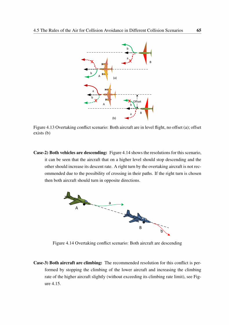
4.5 The Rules of the Air for Collision Avoidance in Different Collision Scenarios 65
A
B
A
B
b
Offset
(a)
(b)
b
b
a
a
xx
xx
b
a
Figure 4.13 Overtaking conflict scenario: Both aircraft are in level flight, no offset (a); offsetexists (b)
Case-2) Both vehicles are descending: Figure 4.14 shows the resolutions for this scenario,it can be seen that the aircraft that on a higher level should stop descending and theother should increase its descent rate. A right turn by the overtaking aircraft is not rec-ommended due to the possibility of crossing in their paths. If the right turn is chosenthen both aircraft should turn in opposite directions.
A
B
a
b
Figure 4.14 Overtaking conflict scenario: Both aircraft are descending
Case-3) Both aircraft are climbing: The recommended resolution for this conflict is per-formed by stopping the climbing of the lower aircraft and increasing the climbingrate of the higher aircraft slightly (without exceeding its climbing rate limit), see Fig-ure 4.15.

66 Decision Making System Based on The Rules of the Air
A
B
a
b
Figure 4.15 Overtaking conflict scenario: Both aircraft are climbing
Case-4) The overtaking aircraft is in level flight, and the overtaken aircraft is climbing:Resolution as in Case-2 (both aircraft are descending) should be performed with theovertaken considering leveling off, and bearing in mind the inertia. This resolutioncan be done when aircraft’s levels are not close or have not already been crossed, seeFigure 4.16.
A
B
a
Figure 4.16 Overtaking conflict scenario:The overtaking aircraft is in level flight, and theovertaken aircraft is climbing
Case-5) The overtaking aircraft is climbing, and the overtaken aircraft is in level flight:Resolution is done by increasing the climb rate of the overtaking aircraft. This reso-lution is possible when the aircrafts’ levels are not close or have not already crossed,see Figure 4.17.
A
B
a
Figure 4.17 Overtaking conflict scenario: The overtaking aircraft is climbing, and the over-taken aircraft is in level flight
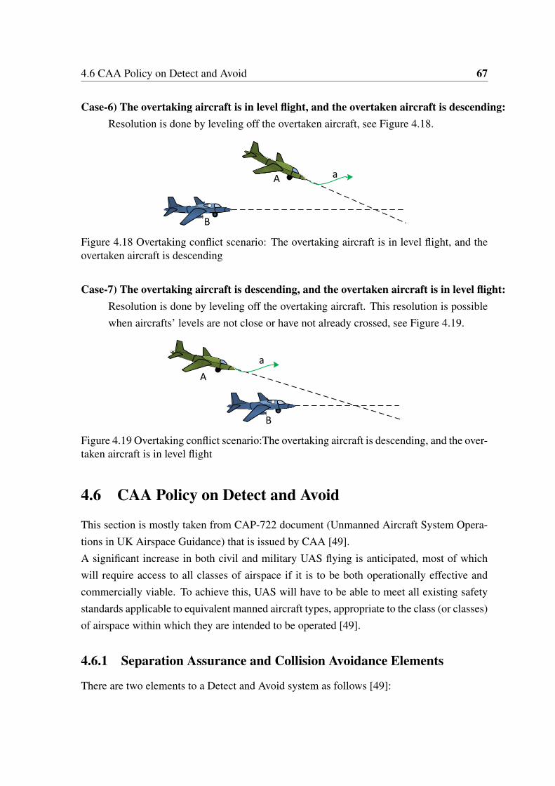
4.6 CAA Policy on Detect and Avoid 67
Case-6) The overtaking aircraft is in level flight, and the overtaken aircraft is descending:Resolution is done by leveling off the overtaken aircraft, see Figure 4.18.
A
B
a
Figure 4.18 Overtaking conflict scenario: The overtaking aircraft is in level flight, and theovertaken aircraft is descending
Case-7) The overtaking aircraft is descending, and the overtaken aircraft is in level flight:Resolution is done by leveling off the overtaking aircraft. This resolution is possiblewhen aircrafts’ levels are not close or have not already crossed, see Figure 4.19.
A
B
a
Figure 4.19 Overtaking conflict scenario:The overtaking aircraft is descending, and the over-taken aircraft is in level flight
4.6 CAA Policy on Detect and Avoid
This section is mostly taken from CAP-722 document (Unmanned Aircraft System Opera-tions in UK Airspace Guidance) that is issued by CAA [49].A significant increase in both civil and military UAS flying is anticipated, most of whichwill require access to all classes of airspace if it is to be both operationally effective andcommercially viable. To achieve this, UAS will have to be able to meet all existing safetystandards applicable to equivalent manned aircraft types, appropriate to the class (or classes)of airspace within which they are intended to be operated [49].
4.6.1 Separation Assurance and Collision Avoidance Elements
There are two elements to a Detect and Avoid system as follows [49]:

68 Decision Making System Based on The Rules of the Air
Separation Assurance This term is used to describe the routine procedures and actionsthat are applied to prevent aircraft getting into close proximity with each other. Anyresolution manoeuvring conducted at this stage must be conducted in accordance withthe rules of the air. When flying in airspace where the provision of separation is theresponsibility of ATC, however, the Remote Pilot should only manoeuvre the aircraftafter receiving ATC approval to do so, in the same fashion as is done for a mannedaircraft.
Collision Avoidance. This is the final layer of conflict management and is the term used todescribe any emergency manoeuvre considered necessary to avoid a collision; such amanoeuvre may contradict the rules of the air or ATC instructions. While the remotepilot would normally be responsible for initiating a collision avoidance manoeuvre,an automatic function may also be required in order to cater for collision avoidancescenarios where the Remote Pilot is unable to initiate the manoeuvre in sufficient time(due to C2 latency issues or lost link scenarios).
The separation and collision avoidance capabilities must be able to [49]:
1. Detect and avoid traffic (air and ground operations) in accordance with the rules ofthe air;
2. Detect and avoid all airborne objects, including gliders, hang-gliders, paragliders,microlights, balloons, parachutists etc;
3. Enable the remote pilot to determine the in-flight meteorological conditions;
4. Avoid hazardous weather;
5. Detect and avoid terrain and other obstacles; and
6. Perform equivalent functions, such as maintaining separation, spacing and sequencingthat would be done visually in a manned aircraft.
4.6.2 Factors for Consideration when Developing a Detect and AvoidSystem for UAS
The CAA Safety Regulation Group does not define the matters to be taken into account forthe design of aircraft or their systems. However, for the guidance of those engaged in thedevelopment of detect and avoid systems, some of the factors that the CAA believes mayneed to be considered are listed below [49].

4.6 CAA Policy on Detect and Avoid 69
1. Ability to comply with the rules of the air.
2. Airworthiness.
3. Control method, controllability and manoeuvrability.
4. Flight performance.
5. Communications procedures and associated links.
6. Security.
7. Emergency actions, reversionary or failure modes in the event of degradation of anypart of the UAS and its associated control and/or relay stations.
8. Actions in the event of lost communications and/or failure of on-board detect andavoid equipment.
9. Ability to determine real-time meteorological conditions and type of terrain beingoverflown.
10. Nature of task and/or payload.
11. Autonomy of operation and control.
12. Method of sensing other airborne objects.
13. Remote pilot level of competence.
14. Communications with ATS providers, procedures and links with control station.
15. Means of launch/take-off and recovery/landing.
16. Reaction logic to other airspace objects.
17. Flight termination.
18. Description of the operation and classification of the airspace in which it is plannedto be flown.
19. Transaction times (e.g. including delays introduced by satellite links).
20. Address both cooperative and non-cooperative air traffic.
This list is not exhaustive [49].
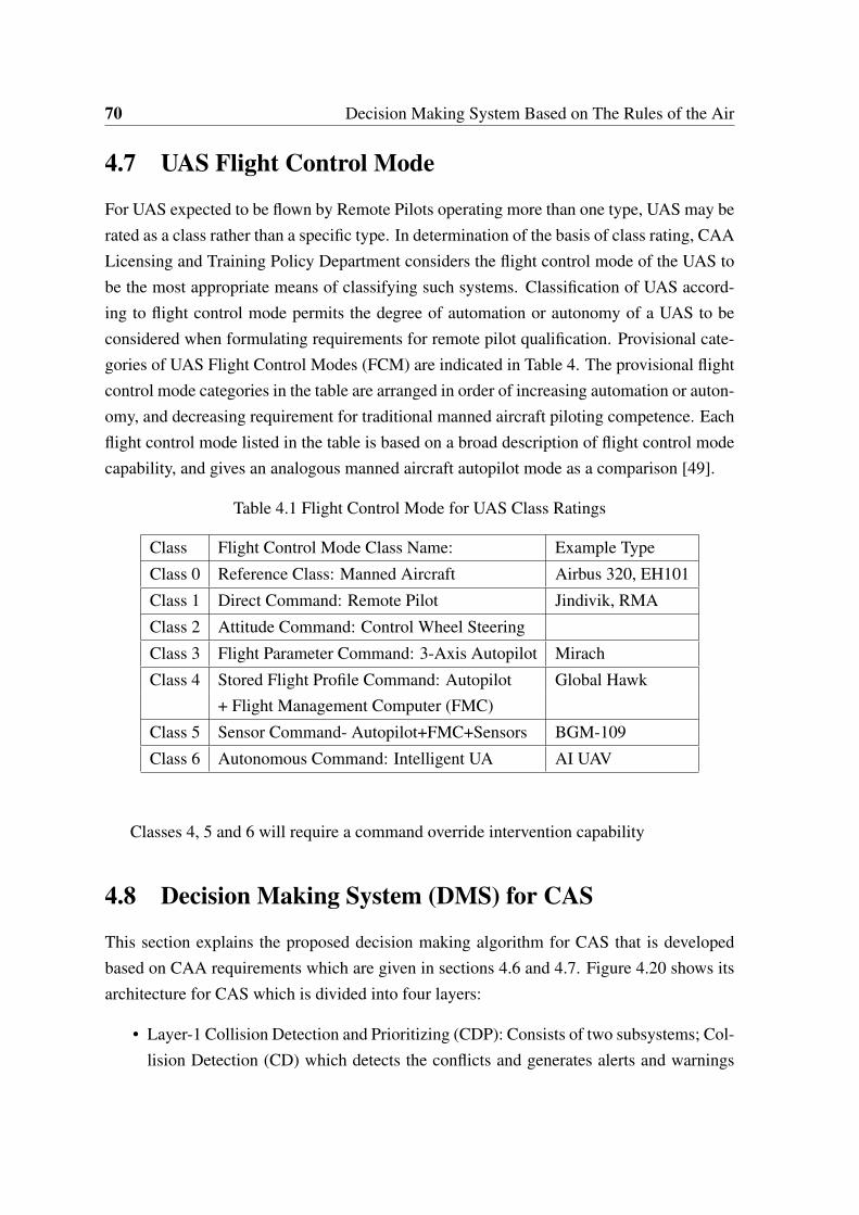
70 Decision Making System Based on The Rules of the Air
4.7 UAS Flight Control Mode
For UAS expected to be flown by Remote Pilots operating more than one type, UAS may berated as a class rather than a specific type. In determination of the basis of class rating, CAALicensing and Training Policy Department considers the flight control mode of the UAS tobe the most appropriate means of classifying such systems. Classification of UAS accord-ing to flight control mode permits the degree of automation or autonomy of a UAS to beconsidered when formulating requirements for remote pilot qualification. Provisional cate-gories of UAS Flight Control Modes (FCM) are indicated in Table 4. The provisional flightcontrol mode categories in the table are arranged in order of increasing automation or auton-omy, and decreasing requirement for traditional manned aircraft piloting competence. Eachflight control mode listed in the table is based on a broad description of flight control modecapability, and gives an analogous manned aircraft autopilot mode as a comparison [49].
Table 4.1 Flight Control Mode for UAS Class Ratings
Class Flight Control Mode Class Name: Example Type
Class 0 Reference Class: Manned Aircraft Airbus 320, EH101
Class 1 Direct Command: Remote Pilot Jindivik, RMA
Class 2 Attitude Command: Control Wheel Steering
Class 3 Flight Parameter Command: 3-Axis Autopilot Mirach
Class 4 Stored Flight Profile Command: Autopilot Global Hawk+ Flight Management Computer (FMC)
Class 5 Sensor Command- Autopilot+FMC+Sensors BGM-109
Class 6 Autonomous Command: Intelligent UA AI UAV
Classes 4, 5 and 6 will require a command override intervention capability
4.8 Decision Making System (DMS) for CAS
This section explains the proposed decision making algorithm for CAS that is developedbased on CAA requirements which are given in sections 4.6 and 4.7. Figure 4.20 shows itsarchitecture for CAS which is divided into four layers:
• Layer-1 Collision Detection and Prioritizing (CDP): Consists of two subsystems; Col-lision Detection (CD) which detects the conflicts and generates alerts and warnings

4.8 Decision Making System (DMS) for CAS 71
flags; and Risks Prioritizing (RP) which defines which of the detected intruders has agreater threats than the others.
• Layer-2 Collision Assessment (CA): Detriments the collision scenario type (i.e. head-on, left/right approaching, and overtaking/overtaken).
• Layer-3 Advisory System (ADS): Gives general conflict resolution advisories (e.g.turn right, turn left, climb, descend, level, and hold speed and altitude)
• Layer-4 Avoidance Manoeuvre Generator (AMG): This layer generates avoidancemanoeuvre that allows the aircraft to avoid the collision.
Layer-2Collision Assessment
Layer-3Advisory System
Layer-4Manoeuvre Generator
HMI(Avionics)
Guidance & Control System
UAV & IntrudersStates
DMS
Risk Prioritizing
Collision Detection
Layer-1
Figure 4.20 DMS architicture
The proposed DMS architecture is engineered to be implemented for different functionali-ties for manned aircraft, and at different level of autonomy of UAS, or at different classes of

72 Decision Making System Based on The Rules of the Air
the flight control mode that given in table 4.1. For example, in Class-0 or manned aircraftthe DMS can be used to reduce the overall pilot workload by performing the flowing tasks:
• Collisions detection and risk prioritizing (Layer-1), so the pilot will know where thetraffics is.
• Determines the collision scenario type (i.e. head-on, left/right approaching, and over-taking/overtaken) by using (Layer-1, and Layer-2) this will help the pilot to decidewhat actions are needed to avoid the conflict.
• Evaluates the collision type, and generates conflict resolution advisories (Layer-3) tohelp the pilot to initiate a suitable avoidance manoeuvre.
For the remotely piloted UAV (Class-1) this architecture helps the remote pilot to build apicture for the surrounding conflicts so the remote pilot could act in the same manner as anon-board pilot. Moreover, the remote pilot can switch to the highly autonomous mode byengaging Layer-4 which generates the avoidance manoeuvre. Layer-4 can be used also inflight mode classes (2-6). The next subsections give a description of the DMS layers.
4.8.1 Collision Detection Layer
This system generates Alert Flags (AF1, AF2), Collision Flag (CF), and gives general infor-mation about the collision risks, such as the intruder direction. According to the rules of theair that were discussed in Section 4.3
A collision risk exists when one aircraft is at the same level or approaching another, its
range is decreasing and its relative bearing remains constant.
So the collision detection unit uses the range, the range rate, the relative altitude, andthe bearing rate as inputs. The outputs are separation alert flags (AF1, AF2) that will beactivated for the aircraft which their range and relative altitude are lees than specific values(loss of separation), collision flag (CF) (active when the bearing angle is constant whichmeans a collision risk exists). Figure 4.21 shows the ranges and the relative altitudes aroundthe aircraft. For safety reasons different ranges and relative altitude can be used to generatetwo types of alerts (R1, and L1 are used to activate AF1); (R2, and L2 are used to activateAF2). Having two levels of alert may help increasing the safety and it may help the pilotto prioritize the intruders in case of multi-intruder scenarios. However, this feature can beswitched off simply by selecting R1 =R2, and L1 = L2. Some commercial Portable Collision

4.8 Decision Making System (DMS) for CAS 73
Avoidance Systems (PCAS) like XRX [75] gives the user the ability to control the valuesof the range and the relative altitude. For example, the range can be selected to be 6 NM, 3NM, or 1.5 NM ( 1 NM = 1850 m), and the relative altitude can be ±2500 feet, ±1500 feet,or ±500 feet. Figure 4.22 shows the flowchart of the algorithm that is used in the collisiondetection system.
L2
L2
L1
L1
R1
R2R2
R1
R2
R1
R2
Figure 4.21 Range, and relative altitude: Horizontal plane (upper); Vertical plane (lower)
4.8.2 Prioritizing
In multi-intruder scenarios it is important to define which intruder should be given a higherpriority than the others so it can be avoided first. The proposed algorithm that is used forprioritizing intruders is similar to that is used in XRX PCAS [75]. However, a commercialPCAS is designed for manned aircraft (class 0 in FCM table 4.1) so for remotely pilotedUAV (class 1) a greater safety margin should be taken due to the Communication and Con-

74 Decision Making System Based on The Rules of the Air
start
AF1=1
End
End
End
Bearing Rate=0
CF=1
Yes
End
Yes
AF2=1
No Yes
No
EndNo
Range<R2&
Relative altitude<L2
No
d(Range)/dt<0
Range<R1&
Relative altitude<L1
Yes
Bearing rate; Range Relative altitude
d(Range)/dt
Figure 4.22 Flowchart of the collision detection system
trol (C2), and data link problems and delay [2]. In this thesis three levels of alerts andwarning (AF1, AF2, CF) are proposed in order to give the remote pilot (class 1 in FCM)more time and greater safety margin so that could overcome the problems that may be asso-ciated with C2 link. The remote pilot can modify the values of ranges and relative altitudesdepend on the UAV manoeuvrability and the flight environment. The prioritizing processcan simply be determined by the following factors:
• Intruder range and relative altitude
• Intruder vertical speed (climbing or descending)
• Aircraft vertical speed (climbing or descending)
While the intruder with (CF) flag has the highest priority above all the intruders, the intruderwith (AF1) flag has the lowest priority. If the intruders have the same flag the intruder withthe least vertical separation (relative altitude) has higher priority. However, if the aircraftis descending/climbing the the relative altitude sign will be taken in consideration. Forexample, if there are two intruders in level flight and both are within ±L2 and both have(AF2) flag, the intruder at higher level will be given higher priority if the aircraft is climbing,but it will given lower priority if the aircraft is descending. The intruders will be given anumber based on their priority, the higher the priority the smaller the number that will begiven. For instance Figure 4.23 shows a conflict scenario in which the three intruders (A, B,
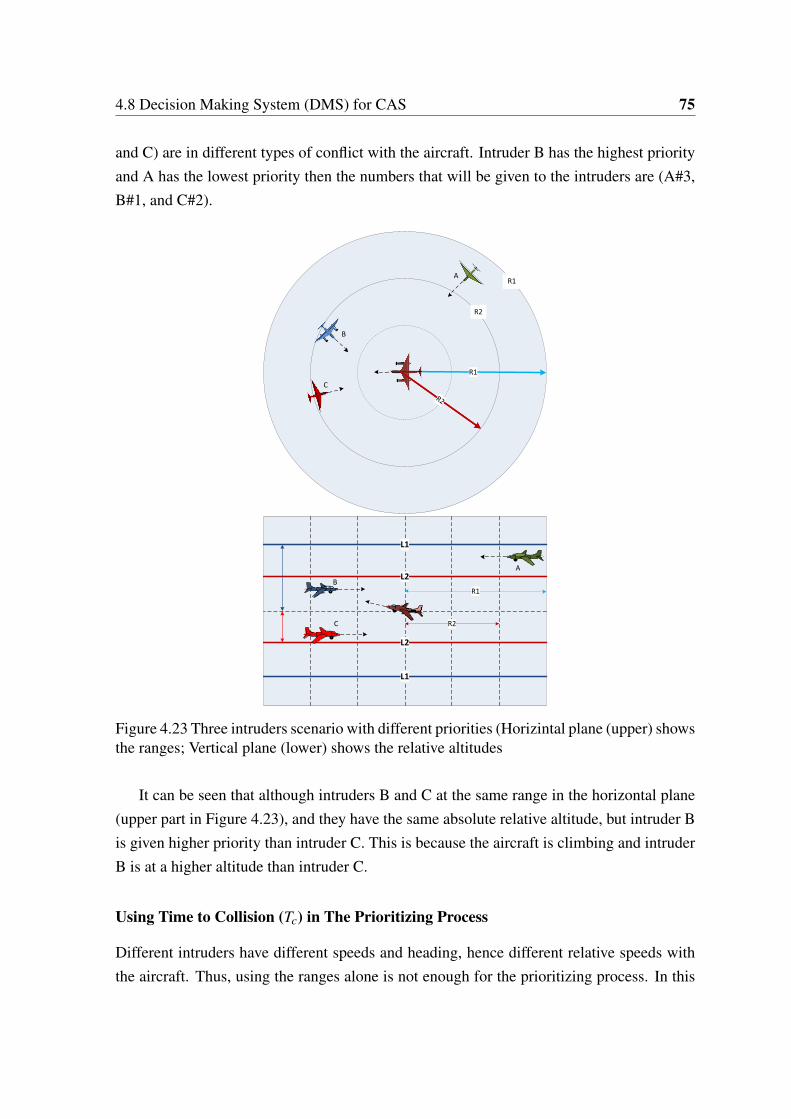
4.8 Decision Making System (DMS) for CAS 75
and C) are in different types of conflict with the aircraft. Intruder B has the highest priorityand A has the lowest priority then the numbers that will be given to the intruders are (A#3,B#1, and C#2).
L2
L2
L1
L1
R1
R2R2
R1
R2
R1
R2
A
B
A
B
C
C
Figure 4.23 Three intruders scenario with different priorities (Horizintal plane (upper) showsthe ranges; Vertical plane (lower) shows the relative altitudes
It can be seen that although intruders B and C at the same range in the horizontal plane(upper part in Figure 4.23), and they have the same absolute relative altitude, but intruder Bis given higher priority than intruder C. This is because the aircraft is climbing and intruderB is at a higher altitude than intruder C.
Using Time to Collision (Tc) in The Prioritizing Process
Different intruders have different speeds and heading, hence different relative speeds withthe aircraft. Thus, using the ranges alone is not enough for the prioritizing process. In this

76 Decision Making System Based on The Rules of the Air
thesis time to collision (Tc) is used in prioritizing process, the smaller the Tc, the higher thepriority will be given. However, the range is implicit in the time to collision, as time tocollision is given by:
Tc =RaVr
(4.1)
where Ra is the range, and Vr is the relative speed or closure rate Vr =d(Ra)
dt . A conflictscenario shown in Figure 4.24 clarifies the importance of using (Tc) in the prioritizing pro-cess. In this scenario the aircraft and the intruders (A, and B) are in level flight at the samealtitude. Initially the intruders’ ranges and speeds are equal, with constant bearing angle forboth, so both have collision flag (CF=1). It is clear that the closure rate of the intruder (B)is greater than the closure rate of the intruder (B) so (TcB < TcA). Hence, using range andrelative altitudes for prioritizing is not enough or even it will give the wrong priority for theintruders (if the range of (A) is less than (B) range). In this example, the intruder with thesmaller Tc which is the intruder (B) is given higher priority than the intruder (A).
4.8.3 Displaying Conflicts Data
Designing a display (Human machine interface (HMI), or avionics) that satisfies the CAArequirements is not in the scope of this thesis. However, a basic Graphic User Interface(GUI) is developed for the purpose of algorithm testing and simulation. Current commer-cial systems display the data in different ways. For example, Figure 4.25 shows the XRXversion of a portable collision avoidance system [75] (PCAS, which is a trademark of ZaonFlight Systems Inc). Figure 4.26 shows the display of the XRX which can show three intrud-ers at the same time, putting the intruder with the highest priority (Primary intruder#1) onthe left side of the screen, and the intruder with the lowest priority (Secondary intruder#2)on the right side of the screen. It gives some information about the intruders such as, the di-rection, range, the relative altitude, and the vertical trend indicator (Climbing/Descending).Figure 4.27 shows the proposed (GUI), the layout of the GUI is designed based on theintruder priority:
• A vertical layout is chosen to represent the intruder priority (The intruder with thehighest priority is at the top of the screen and the intruder with the lowest priority atthe bottom of the screen).
• The size of the intruder display reflects the intruder priority, the higher the priority thebigger the size of the intruder display.

4.8 Decision Making System (DMS) for CAS 77
L2
L2
L1
L1
R1
R2R2
R1
R2
R1
R2
A
AB
B
Figure 4.24 Conflict scenario clarifying the importance of the Tc in the prioritizing process
• The higher the intruder priority the more information is displayed.
• The accuracy of the bearing angle of the intruder (intruder direction) is increased asthe intruder priority is increased.
• The relative altitude is represented numerically and graphically.
The proposed GUI can be a ground for a future research for further development to be afully certified HMI.
Figure 4.28 shows how the GUI looks like (right) in case of a conflict scenario whichis given on the left. Intruder C has the highest priority so its information are displayed onthe to display, while intruder B has the lowest priority then it is appear on the display at thebottom. Intruder C bearing is more than 0◦, but lees than 30◦ so two direction indicatorsare highlighted.

78 Decision Making System Based on The Rules of the Air
Figure 4.25 PCAS XRX
Primary intruder
Secondary intruder #1
Secondary intruder #2
Aircraft heading Aircraft altitudeClimbing/
Descending
Relative altitude Intruder
direction
Intruder range
1.9-06
3.0 5.0-09 +12
HDG 360 FL 037
Figure 4.26 PCAS XRX display
4.8.4 Collision Assessment Layer
The collision information of the intruder with the highest priority is passed to collisionassessment layer (Layer-2) and the assessment algorithm is applied in order to determinethe conflict type. Heading angles of the aircraft and the intruder, and bearing angle is usedin the assessment process. Sections 4.4 and 4.5 described different conflict scenarios andshowed how to differentiate between them by using the bearing angle (see figure 4.3). Forexample, if the intruder is approaching within (±45◦) it will be considered as a head-oncollision. However, an offset scenario is considered just when the difference between the

4.8 Decision Making System (DMS) for CAS 79
The in
trud
er with
the
high
est prio
rity
The intruder with the lowest priority
Climb/Descend rate [m/s] or [f/min]
The intruder direction indicator
Relative altitude [m or feet]x100
Climb/Descend indicator
Relative altitude indicator The in
trud
er with
the
secon
d to
p p
riority
45
Figure 4.27 Displaying Layer-1 output on GUI/ Avionics
heading angle of the aircraft and the intruder is (180◦) and the intruder is on the right of thecenterline of the aircraft (see Figure 4.7). If the aircraft and the intruder position in the earthaxis reference frame (North, East, Up (NEU) reference frame) are known then the intruderrange and bearing can be calculated. Figure 4.29 shows the aircraft and the intruder in theNEU reference frame. The body reference frame [o,xb,yb,zb]
T is attached to the aircraftand is used to convert the intruder position values from the NEU reference frame into theaircraft body reference frame using the Directional Cosine Matrix (DCM) then:
Ra =√
Hrange2 +Vrange
2 (4.2)
Bearing is calculated in the horizontal plane as the vertical bearing can be ignored (rel-ative altitude is small enough to be ignored comparing to the range). So if [xe,ye]
T are theintruder position in the horizontal plane in NEU reference frame, and the aircraft heading is

80 Decision Making System Based on The Rules of the Air
L2
L2
L1
L1
R1
R2R2
R1
R2
R1
R2
A#2
B#3
B#3
C#1
A#2
C#1
32
Figure 4.28 Conflict scenario (left), and its displayed information on GUI/Avoinics (right)
ψ , the intruder position in the horizontal plane in the aircraft reference frame [x1b,y1b]T is
given as: [x1b
y1b
]= DCM
[xe
ye
](4.3)
where DCM is the directional cosine matrix:
DCM =
(cos(ψ) sin(ψ)
−sin(ψ) cos(ψ)
)(4.4)
So bearing is given by:Br = atan2(y1b,x1b) (4.5)
Figure 4.30 shows the flowchart for the proposed collision assessment algorithm. This al-gorithm is developed based on Figure 4.3, the bearing is used to assess the approaching
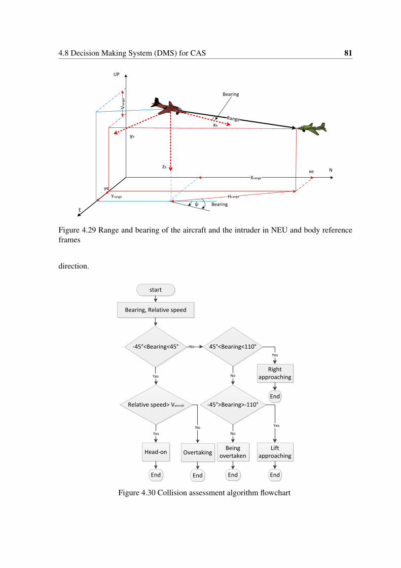
4.8 Decision Making System (DMS) for CAS 81
Range
N
E
UP
ψ
xb
xe
ye
yb
zb
Bearing
Hrange
Bearing
Vra
nge
Xrange
Yrange
Figure 4.29 Range and bearing of the aircraft and the intruder in NEU and body referenceframes
direction.
start
Bearing, Relative speed
-45°<Bearing<45°
Relative speed> Vaircraft
Head-on
Yes
End
End
EndEnd
Yes
No
No
Overtaking
45°<Bearing<110°
Right approaching
Yes
No
-45°>Bearing>-110°
Lift approaching
Yes
No
Being overtaken
End
Figure 4.30 Collision assessment algorithm flowchart

82 Decision Making System Based on The Rules of the Air
However, when the bearing is (±45◦), relative speed between the aircraft and the intruderis used to differentiate between head-on and overtaking conflict scenarios:
• Head-on conflict scenario, if relative speed is greater than the aircraft speed.
• Aircraft is overtaking the intruder conflict scenario, if the relative speed is smallerthan the aircraft speed.
The information that will be passed to the pilot (in manned aircraft), or the remote pilot incase of UAV are collision type (i.e. Head-on, right/left approaching, overtaking, and beingovertaken), the relative speed or closure rate Vr, and the time to collide Tc. Figure 4.31 showsthe proposed GUI/avionics layout for showing information that is generated by Layer-2.
L2
L2
L1
L1
R1
R2R2
R1
R2
R1
R2
A#2
B#3
B#3
C#1
A#2
C#1
32
Head-on
25 s
85 m/s
C-TypeC-Type
TC
Vr
Figure 4.31 Conflict scenario (left), GUI with Layer-1, and Layer-2 information (right)
It is important for the pilot to know Tc in order to initiate the avoidance manoeuvre.The required time for a pilot to recognise an approaching aircraft and initiate an avoidancemanoeuvre is divided as follows [7]:

4.8 Decision Making System (DMS) for CAS 83
• See object (0.1 second)
• Recognise aircraft (1 second)
• Recognise collision (5 second)
• Decision to turn right or left action (4 second)
• Muscular reaction lag time (0.4 second)
• Aircraft lag time (2 second)
Thus the total time is (12.5 second) which is the minimum time for the pilot to detect theintruder prior to the time of impact to have a chance of avoiding a collision. However, thistime may increased as pilots differ in their response time, the reaction time for less experi-enced or older pilots is likely to be greater than (12.5 second) [8]. Pilots use their experienceand the size of the intruder to determine the time to collision. Figure 4.32 represents an air-craft as it would appear to the pilot from the distances indicated in the table on the left [7].The required time to cover these distances is given in seconds for relative speed of 600 mphand 210 mph.
Distance TC [s] TC [s]
600 mph 210 mph
10 miles 60 170
5 miles 30 85
3 miles 18 56
2 miles 12 38
1 mile 6 13
0.5 3 9
Figure 4.32 Aircraft closure rate chart
84 Decision Making System Based on The Rules of the Air
Two flags are generated by the collision assessment system:
1. The intruder at Nine O’clock Flag (NF): This flag is activated when the intruder be-come at at 9 o’clock position relative to the UAV. NF will be used by the avoid-ance manoeuvre generation system. This will be discussed in more detail in the nextchapter (see Section 5.2.3). In some conflict avoidance scenarios (e.g. Approachingconflict scenarios) in manned aircraft the pilot observes the intruder position whileperforming the avoidance manoeuvre, and when the intruder reaches the 9 o’clockposition the pilot tries to restore the initial heading angle of the aircraft. Hence, theaircraft flies parallel to its previous path.
2. Collision Resolved Flag (RF): This flag is activated when the collision is resolved.The collision is resolved if the intruder range is greater than a predefined value, andthe relative speed or closure Vr is positive. RF flag is used for algorithm resettingpurposes (see Sections 5.2.2, and 5.2.3).
4.8.5 Advisory System
Layer-1 and Layer-2 functions (shown in Figure 4.20) are data collection and assessmentwithout any decision making functionality. Layer-3 is the first layer that has the decisionmaking functionality in the DMS architecture. It uses the information that is generated byLayer-1 and Layer-2 with the rules of the air to generate the suitable Resolution Advisories(RA) which can be used by pilot or the remote pilot to avoid the conflict. In this thesis thelevel flight scenario is discussed so the horizontal advisories for avoidance manoeuvres aregenerated which are:
• Turn right manoeuvre: If AF1=1 and AF2=0 then the the RA is single (Right), but if(AF2=1 or CF=1) then the RA command is double (Right, Right) indicating that thepilot should make a greater right turn than the single (Right) command.
• Turn left manoeuvre: Same as turn right case so if AF1=1 then (Left); if AF2=1 orCF=1 then (Left,Left).
• Holding the current speed and altitude: The RA in this case is (Hold)
• Level off
• Descend or increase/decraese descending rate: (Descend) means the pilot should initi-ate descending manoeuvre, (Decrease/Increase Descend) for decreasing or increasingdescending rate.

4.8 Decision Making System (DMS) for CAS 85
• Climb or increase/decrease climbing rate:(Climb) means the pilot should initiate climb-ing manoeuvre, (Decrease/Increase Climb) for decreasing or increasing climbing rate.
Figure 4.33 shows the flowchart for the advisory algorithm that is used in head-on collisionscenarios. It can be seen that when (AF2) is not activated (which means that the intruder isfar enough away to make vertical manoeuvre) if the aircraft is climbing or descending theRA command is to level off the aircraft. But if the aircraft is in level flight then the RAis (Right) in case there is no offset, and (Left) in the offset case. However, if (AF2 or CF)are activated then the vertical resolution advisories will not be taken into consideration forsafety reasons due to the aircraft inertia in vertical manoeuvre. So the advisory system willjust generate the horizontal resolution advisories which are (Right, Right) when no offsetexists and (Left, Left) in the case of offset.
Start
AF2=1Turn rightAircraft descending
Or climbingNoOffset=1 YesNo
Turn left
Yes
Level offYes
End
End
End
Head-on
Turn right Offset=1No
Turn left
Yes
End
End
NO
Issued advisories are:1-(Right, Right): for right manoeuver 2- (Left, left) for left manoeuver
Issued advisories are:1-(Right): for right manoeuver 2- (Left) for left manoeuver
Figure 4.33 Flowchart for advisory generating during head-on collision
The purpose of using a single or double word when generating the resolution advisoriesis to give the pilot an indication of the level of the risk, hence the pilot takes this intoaccount when initial an avoidance manoeuvre. For example, the turn rate (in case of a hor-izontal avoidance manoeuvre), when double word is issued by the advisory system, shouldbe greater than the turn rate in case of single word command. Figure 4.34 gives the flowchartfor the advisory algorithm that generates the resolution advisories in (overtaking, and being

86 Decision Making System Based on The Rules of the Air
overtaken) scenarios. In this flowchart (Ralt) refers to the relative altitude, where the altitudeof the overtaking aircraft is the reference. For the same reason that has been discussed inhead-on scenarios the vertical resolution advisories are taken into consideration just in case(AF1=1, and AF2=0).
Start
AF2=1
Overtaking: descending
Offset=1 No
YesEnd
Overtaking/Overtaken
Issued advisories are:1-(Right, Right): for right manoeuver 2- (Left, left) for left manoeuver3- (Hold): for holding current speed and level
Issued advisories are:1-(Level Off) 2- (Increase Descend) for increasing descending rate3- (Increase Climb) for increasing climbing rate4- Hold Off: for holding current level and speed
Overtaken: Descending or
level flight
Yes
Ralt<0
Yes
Overtaking: Level offOvertaken: Increase Descend rate
Yes
Overtaking: Increase Descend rateOvertaken: Level off
No
Overtaking: Climbing
Overtaken: Climbing
Yes
Ralt>0
Yes
Overtaking: Level offOvertaken: Increase climb rate
NoOvertaking: Increase climb rateOvertaken: Level off
Yes
Overtaken: Climbing or descending
No
Overtaken: Level flight
No
Yes
End No
End
So the Overtaking aircraft in level
flight
Overtaking: Keep Level flightOvertaken: Level off
Yes
No
No
No
Overtaking: RightOvertaken: Hold current speed and level
Overtaking: LeftOvertaken: Hold current speed and level
1No
Yes
Offset=1
Issued advisories are:1-(Right): for right manoeuver 2- (Left): for left manoeuver3- (Hold): for holding current speed and level
Overtaking: RightOvertaken: Hold current speed and level
Overtaking: LeftOvertaken: Hold current speed and level
1
Yes
No
Figure 4.34 Flowchart for RA generation for overtaking/overtaken conflict scenarios

4.8 Decision Making System (DMS) for CAS 87
The conflict resolution advisories can be passed to the GUI unit in case of the remotelypiloted UAV, or can be shown on the avionics for manned aircraft. Figure 4.35 shows theproposed layout for the GUI which displays the advisories as a text (e.g. Right; Left; Right,Right; Descend/Climb; Hold; Level Off), the resolution advisories are shown graphicallyusing arrows to indicate the avoidance manoeuvre direction (Right/Left arrows), and thevertical advisories (Up arrow for climbing, and down arrow for descending) the length ofarrows represents the value of turning, climbing, and descending that should be initiated bythe pilot. The Auto/Manual command bottom gives the remote pilot two options:
• Manual: The pilot is responsible for performing the avoidance manoeuvre.
• Auto: The UAV is operating in highly autonomous mode where the avoidance ma-noeuvre is generated by CAS.
The manoeuvre generation layer (Layer-4) gives the proposed DMS the (Auto) functionalitywhich will be discussed in more detail in the chapters 5 and 6.
L2
L2
L1
L1
R1
R2R2
R1
R2
R1
R2
A#2
B#3
B#3
C#1
A#2
C#1
32
Head-on
25 s
85 m/s
C-TypeC-Type
TC
Vr
Right
Resolution
Auto/Manual
Figure 4.35 GUI/Avionics layout including the conflict resolution advisories
88 Decision Making System Based on The Rules of the Air
4.8.6 Avoidance Manoeuvre Generation
Avoidance manoeuvre generation is the final step in the proposed DMS. In order to makethe UAV behave the same as a manned aircraft during the conflict scenarios, the generatedavoidance manoeuvre must be compliant with the rules of the air. The avoidance manoeuvregeneration layer uses the information from the upper layers in the DMS, and the rules ofthe air to generate the avoidance manoeuvre trajectory profiles. A predefined manoeuvreshape is used for generating the avoidance manoeuvre trajectory profiles. The predefinedmanoeuvre parameters are calculated based on the UAV and the intruder initial states, andthe UAV dynamics constraints. The next chapter discusses in more detail the avoidancemanoeuvres generation process for different conflict scenarios.
4.9 Summary
This chapter proposes a decision making system (DMS) algorithm for the collision avoid-ance systems (CAS). Firstly, a brief description of airspace classes, the rules of the air, andhow aircraft should behave during collision avoidance in different conflict scenarios is pro-vided. Then a decision making system (DMS) for collision avoidance is developed basedon the rules of the air in VFR conditions and CAA requirements. The DMS is divided intomultiple-layers, each layer is built to perform a specific function. The different functionsthat should be performed by the DMS layers are presented (e.g. conflict detections, priori-tizing, and assessment). A graphical user interface (GUI) is proposed for algorithm testingand simulation purposes with a short comparison with currently used commercial PortableCollision Avoidance System (PCAS).
Chapter 5
Avoidance Manoeuvre Generation
5.1 Introduction
Avoidance manoeuvre generation is the final step in the proposed Decision Making System(DMS) that discussed in chapter 4. In order to make the UAV behave the same as a mannedaircraft during the conflict scenarios the generated avoidance manoeuvre must be compli-ant with the rules of the air. This chapter discusses the avoidance manoeuvres generationprocess for different conflict scenarios in which the UAV changes direction (right/left turn)in a horizontal manoeuvre. Two conflict scenarios are discussed head-on/overtaking, andright approaching. Although the rules of the air give general instructions for avoiding thedifferent conflict scenarios, there are no specific procedures for performing the avoidancemanoeuvres. However, pilots use their experience to comply with the rules of the air.
The proposed avoidance manoeuvre generation process uses the information from theupper layers in the DMS and the rules of the air to generate the avoidance manoeuvre tra-jectory profiles. A predefined manoeuvre shape is used for generating the avoidance ma-noeuvre trajectory profiles. The predefined manoeuvre parameters are calculated based onthe UAV and the intruder initial states together with the UAV dynamics constraints. For ex-ample, a combination of level flight and a coordinated turn manoeuvre with constant speedand altitude is selected for the horizontal avoidance manoeuvres. The coordinated turn ma-noeuvre is defined by the heading rate values during a period of time. Thus, the avoidancemanoeuvre time is divided into periods of time each one associated with a specific value ofheading rate (while the heading rate of coordinated turn has a non-zero constant value, it iszero in level flight). As the time periods are specified with their associated heading rate val-ues the overall heading rate signal can be constructed. The avoidance manoeuvre trajectory

90 Avoidance Manoeuvre Generation
profiles are generated by applying the calculated heading rate signal to the UAV dynamicmodel. The generated avoidance manoeuvre trajectory profiles are, then, either passed to theinverse dynamics to generate the UAV control inputs, or used as global trajectory profilesfor the Local Trajectory Planning (LTP) algorithm that was discussed in Chapter 3. Thesecond option is considered in this thesis (see Section 5.4.1).
5.2 Avoidance Manoeuvre Trajectory Generation
The avoidance manoeuvre trajectory profile generation process can be divided into the fol-lowing steps:
1. Specify the avoidance manoeuvre type and find its characteristics. The coordinatedturn with a constant speed and altitude is selected to be the manoeuvre for the turnpart of the avoidance manoeuvre and the level flight manoeuvre is selected for thestraight flight part of the avoidance manoeuvre.
2. Define the heading rate of the coordinated turn according to the UAV current statesand dynamic constraints (the heading rate for the level flight is zero). Then dependingon the conflict scenario the manoeuvre time periods with the associated heading ratecan be calculated.
3. Construct the heading rate signal and apply it to the UAV dynamic model to generatethe avoidance manoeuvre trajectory profiles (position, and speed profiles).
4. The generated avoidance manoeuvre trajectory profiles can be used as global trajec-tory profiles for the Local Trajectory Planner (LTP) algorithm, or they can be passeddirectly to the inverse dynamic algorithm to generate the UAV command inputs.
5.2.1 Coordinated Turn with Constant Speed and Altitude
The coordinated turn with a constant speed and altitude is proposed for the turning part ofthe avoidance manoeuvre (selected based on pilot suggestions). Pilots prefer this type ofmanoeuvre for several reasons [65]:
• The constant speed means the coordinated turn is desirable for passenger comfort.
• It allows the pilot to function more effectively.

5.2 Avoidance Manoeuvre Trajectory Generation 91
• It maintains maximum aerodynamic efficiency by minimizing sideslip and also mini-mizing undesirable aerodynamic loading of the structure.
• In the case of a remotely piloted UAV the turn coordination is useful for performingvideo surveillance or targeting.
• In a coordinated turn, level or otherwise, the aircraft maintains the same pitch angleand roll attitude with respect to the reference coordinate, but its heading angle changescontinuously at constant rate. Therefore, the Euler-angle rates φ and θ are identicallyzero, and the turn rate ψ is a non-zero constant value.
Figure 5.1 shows the forces acting on the aircraft when it is flying in a steady level coordi-nated turn at a constant speed V .
Radius of turn R
Bank angle Ø
Lift L
mV2/R
mg
Figure 5.1 Forces balance in equilibrium state of turning aircraft
At an equilibrium state the acting forces on the aircraft are balanced. So the projectionof the lift force on the horizontal axis balances the centrifugal force:
Lsin(φ) =mV 2
R(5.1)
and the projection of the lift force on the vertical axis balances aircraft wight force:
Lcos(φ) = mg (5.2)

92 Avoidance Manoeuvre Generation
hence, the turn radius can be calculated from 5.1 and 5.2:
R =V 2
g tan(φ)(5.3)
The time to complete one turn is:
t =2πRV
=2πV
g tan(φ)(5.4)
Heading rate or rate of turn is given by:
ψ =2π
t= g
tan(φ)V
(5.5)
at a specific speed value the maximum heading rate is:
ψmax = gtan(φmax)
V(5.6)
where φmax is the maximum roll angle. In order to maintain constant altitude and speedduring turning, lift and thrust must be increased to compensate the vertical lift reductionand the increase in the drag. The normal load factor is:
n =L
mg(5.7)
The normal load factor during the turn can be derived from (5.2), and (5.7):
n =1
cos(φ)(5.8)
So the bank angle is limited by the maximum normal load factor:
nmax =12ρV 2SCLmax
mg=
1cos(φmax)
(5.9)
In addition, the stall speed must be taken into consideration in the generation of avoidancemanoeuvre, because it increases during the turn:
Vstallturn =Vstall√
n =Vstall√cos(φ)
(5.10)

5.2 Avoidance Manoeuvre Trajectory Generation 93
where Vstallturn is the stall speed in the turn, Vstall is the stall speed in the level flight. Equa-tion 5.10 shows that as the bank angle is increased the stall speed is increased. Also the loadfactor must be increased to maintain the aircraft altitude.
5.2.2 Avoidance Manoeuvre for Head-on/Overtaking Conflict Scenar-ios
The rules of the air for head-on and overtaking conflict scenarios are discussed in Chapter 4.Depending on the conflict scenario the UAV should avoid the conflict by turning (right/left).The direction of turn is determined by the upper layers of the DMS. The same manoeuvretype is proposed for the head-on and the overtaking conflict scenarios. Figure 5.2 shows theavoidance manoeuvre for a head-on conflict scenario (where the UAV should turn right).The proposed manoeuvre for the head-on/overtaking conflict scenarios are performed asfollows:
1. Turn right: Use a coordinated turn with constant speed V and constant altitude tochange heading angle by a predefined value ∆ψT 1. The constant heading rate duringthis time period (T1) is ψ1.
2. Fly straight: Level flight with constant speed V , then when the achieved lateral dis-tance is greater than a predefined clearance distance dc.
3. Turn left: Using again the coordinated turn with the same turn rate ψ3 =−ψ1 and thesame total change of heading angle ∆ψT 3 =−∆ψT1 .
4. Fly straight: Keep flying parallel to the global trajectory till the collision resolutionflag RF is issued by the collision assessment layer.
The avoidance manoeuvre that is shown in Figure 5.2, can be generated by using the headingrate that is shown in Figure 5.3 as command signal and holding the speed and altitude atconstant values.

94 Avoidance Manoeuvre Generation
CP
ΔΨT1
Clearance distance (dc)
T1 T2 T3 T4
Figure 5.2 The avoidance manoeuvre for the head-on conflict scenario
Heading rate integration gives the heading angle for the selected manoeuvre as shownin Figure 5.4.
ψ
ψmax
ψmax
Tm
T1 T2 T3
Time
ψ1
ψ3
T4
Figure 5.3 The heading rate of the proposed head-on collision avoidance manoeuvre

5.2 Avoidance Manoeuvre Trajectory Generation 95
ψ
Tm
T1 T2 T3
Time
ψ0
ψ1 ψ2
ψ3
ΔψT1=ψ1-ψ0 ΔψT3=ψ3 – ψ2
T4
Ψ
Ψ.
Figure 5.4 The heading angle of the proposed head-on collision avoidance manoeuvre
The proposed avoidance manoeuvre is governed by the selected heading rates (ψ1, ψ3),and the predefined total heading angle changes (∆ψ1, ∆ψ3). The time periods (Tm, T1, T2,T3, T4) can be calculated depending on the heading rates and the total heading angle changeswhich have to satisfy the following conditions:
1. The heading difference ∆ψT1 <π
2 : To prevent the UAV from heading backward duringand after resolving the conflict. This also will guarantee that the intruder will be in theField of Regard (FOR) while the avoidance manoeuvre is performed (the requirementfor the onboard sensor system for UAV is to cover the field of regard of (±110◦)horizontal with respect to the longitudinal axis of the UAV, see Section 2.5.1)
2. The UAV heading should be the same at the start and end of the manoeuvre (ψ0 =ψ3):It can be noted that the change in heading angle occurs during (T1) and (T3), so thiscondition can be achieved by:
∆ψT 3 =−∆ψT1 (5.11)
where ∆ψT1 = T1ψ1, and ∆ψT3 = T3ψ3 are the total heading changes during the timeperiods T1, and T3 respectively so:
T3ψ3 =−T1ψ1 ⇒ψ1
ψ3=−T3
T1(5.12)
in this research ψ3 =−ψ1 , so time periods T1, and T3 are identical.
3. The second time period T2 is selected to allow the UAV to achieve enough clearancedistance from the expected Collision Point (CP), so the clearance distance should begreater or equal to a predefined value dc.
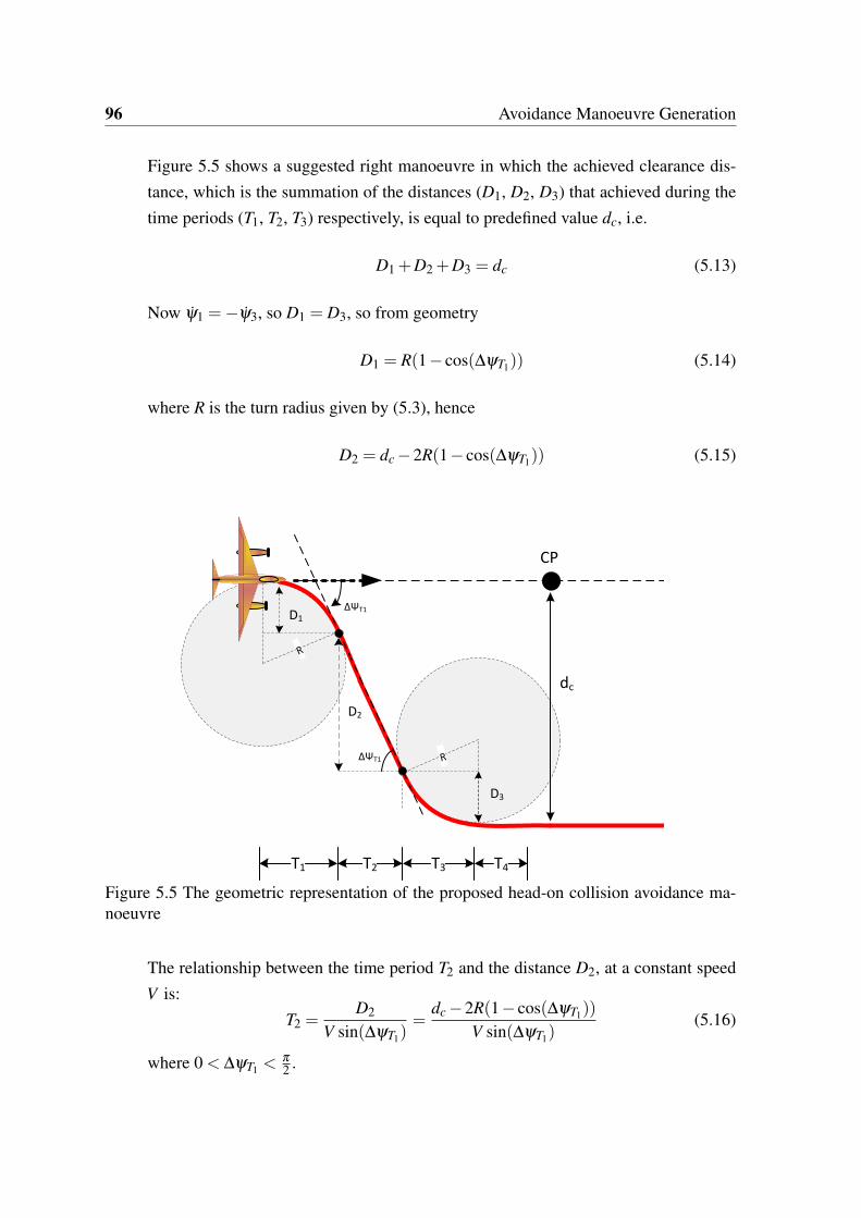
96 Avoidance Manoeuvre Generation
Figure 5.5 shows a suggested right manoeuvre in which the achieved clearance dis-tance, which is the summation of the distances (D1, D2, D3) that achieved during thetime periods (T1, T2, T3) respectively, is equal to predefined value dc, i.e.
D1 +D2 +D3 = dc (5.13)
Now ψ1 =−ψ3, so D1 = D3, so from geometry
D1 = R(1− cos(∆ψT1)) (5.14)
where R is the turn radius given by (5.3), hence
D2 = dc −2R(1− cos(∆ψT1)) (5.15)
R
CP
ΔΨT1
T1 T2 T3
ΔΨT1
D2
D1
D3
R
dc
T4
Figure 5.5 The geometric representation of the proposed head-on collision avoidance ma-noeuvre
The relationship between the time period T2 and the distance D2, at a constant speedV is:
T2 =D2
V sin(∆ψT1)=
dc −2R(1− cos(∆ψT1))
V sin(∆ψT1)(5.16)
where 0 < ∆ψT1 <π
2 .

5.2 Avoidance Manoeuvre Trajectory Generation 97
4. Calculating T4, and Tm: The manoeuvre time Tm is going to be used in the next steps,for instance, in the trajectory profiles discretisation, and in the speed profiles integra-tion for position profile generation. Hence, it must be predefined as a constant value.The constant value of Tm must be enough to perform the avoidance manoeuvre andresolve the collision. The time period T4 can be calculated:
T4 = Tm − (T1 +T2 +T3) (5.17)
It worth mentioning that it is not necessary for the avoidance manoeuvre to take thewhole manoeuvre time Tm, because it may be interrupted when the collision reso-lution flag RF is generated by collision assessment unit as seen in Figure 5.6. Thecollision resolution flag RF is generated when the conflict is resolved as discussed inSection 4.8.4.
0
CF
Tm
T1 T2 T3 T4
RF
Start the avoidance manoeuvreStop the avoidance manoeuvre;Return to the global trajectory
0
Time
ψ1
. .ψ3
Figure 5.6 Avoidance manoeuvre initialization and interruption by CF, and RF
Two variations of the avoidance manoeuvre are proposed: average manoeuvre and exagger-ated manoeuvre. The average manoeuvre is used when the time to collision Tc is within apredefined range value (e.g. greater than 20 sec). The exaggerated manoeuvre is used inthe critical situation when the time to collision is small. In manned aircraft, the pilot usesan exaggerated turn manoeuvre to make the other pilot aware of the collision risk and toperforme the avoidance manoeuvre. Table 5.1 gives the quantities that are used for eachmanoeuvre. Although the avoidance manoeuvres are proposed based on pilot suggestions,the proposed algorithm is not sufficient to allow the UAV to behave the same as a mannedaircraft by generating different manoeuvres for different conflict situations. In a manned

98 Avoidance Manoeuvre Generation
Table 5.1 Average and exaggerated manoeuvre quantities
Quantity Average manoeuvre Exaggerated manoeuvreTc > 20s ≤ 20s
∆ψπ
4π
3ψo [50%−75%]ψmax [75%−100%]ψmax
aircraft the pilot uses his/her experience to initiate a safe avoidance manoeuvre. Thus, afurther development is proposed to use the pilot experience in avoidance manoeuvre gener-ating process. A fuzzy logic technique is proposed to define the roll rate of the avoidancemanoeuvre based on the pilot behaviour during different conflict scenarios. The proposal isdiscussed in more details in the Chapter 6.
5.2.3 Avoidance Manoeuvre for Approaching Scenarios
According to the rules of the air the UAV gives the way to the traffic that is approachingfrom the right side by turning right and tracking behind the approached intruder.
An aircraft which is obliged to give way to another aircraft must avoid passing over
or under, or crossing ahead of, the other aircraft unless passing well clear of it [16] (seeChapter 4).
The proposal in this research is to use the coordinated turn manoeuvre at constant speedand altitude to generate the avoidance manoeuvre for the right approaching conflict scenar-ios. Three types of avoidance manoeuvre are proposed:
1. Right-Straight-Left (RSL) manoeuvre: The UAV turns right by π
2 rad, then travelsstraight until the intruder is at 9 o’clock relative to the UAV (usually pilots use aclock position to give the relative direction of an object), at this point the UAV turnsleft by π
2 rad, so the heading angle will be as same as the UAV when the avoidancemanoeuvre is initiated. Thus, the UAV will be parallel with the global trajectorythat was being tracked before the avoidance manoeuvre was initiated. If the advisorysystem command are issued to turn left first then this manoeuvre is simply becomes aLeft-Strait-Right manoeuvre (LSR)
2. Right-Straight then Left-Straight (RS-LS) manoeuvre: The RSL avoidance manoeu-vre is highly dependent on the intruder states, hence, a developed version of RSLavoidance manoeuvre is proposed to overcome this drawback. The RS-LS avoidance
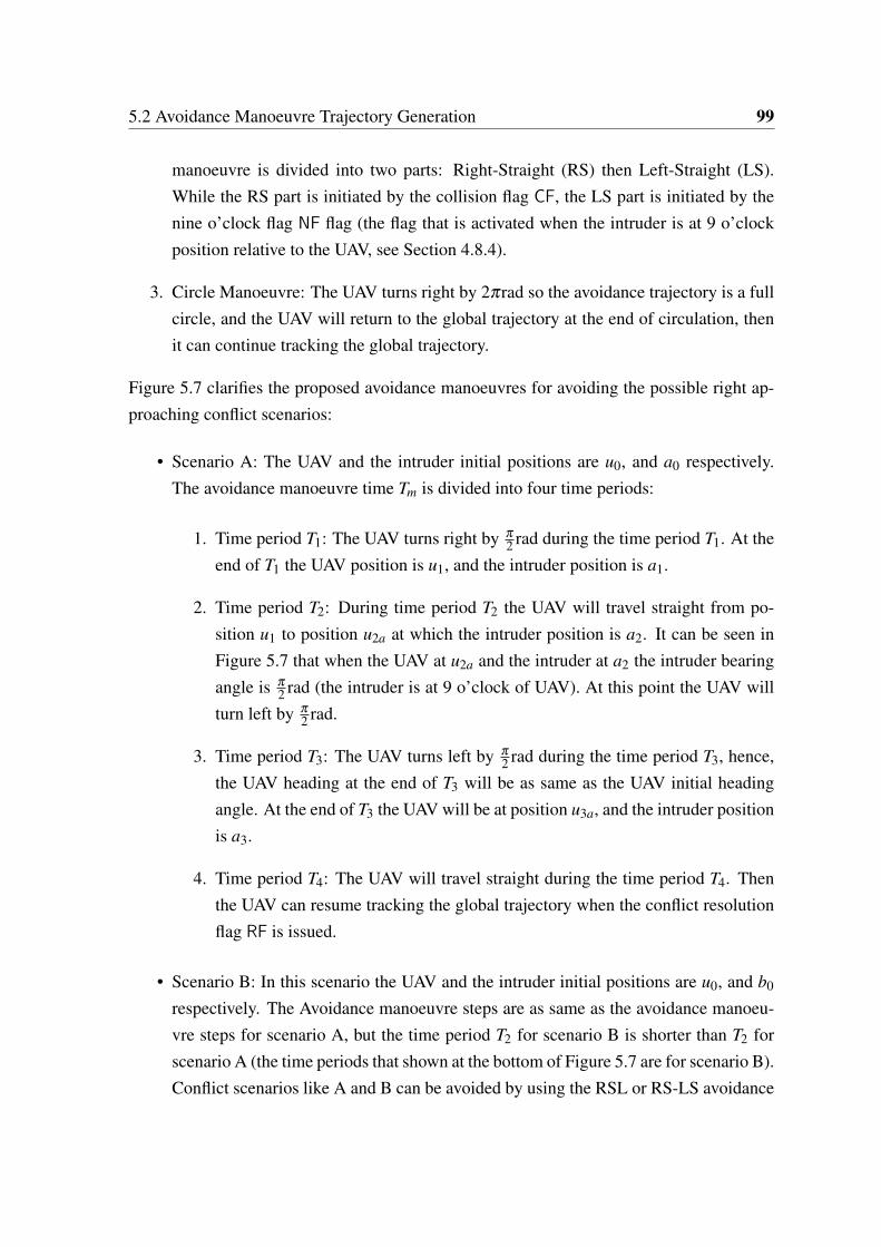
5.2 Avoidance Manoeuvre Trajectory Generation 99
manoeuvre is divided into two parts: Right-Straight (RS) then Left-Straight (LS).While the RS part is initiated by the collision flag CF, the LS part is initiated by thenine o’clock flag NF flag (the flag that is activated when the intruder is at 9 o’clockposition relative to the UAV, see Section 4.8.4).
3. Circle Manoeuvre: The UAV turns right by 2πrad so the avoidance trajectory is a fullcircle, and the UAV will return to the global trajectory at the end of circulation, thenit can continue tracking the global trajectory.
Figure 5.7 clarifies the proposed avoidance manoeuvres for avoiding the possible right ap-proaching conflict scenarios:
• Scenario A: The UAV and the intruder initial positions are u0, and a0 respectively.The avoidance manoeuvre time Tm is divided into four time periods:
1. Time period T1: The UAV turns right by π
2 rad during the time period T1. At theend of T1 the UAV position is u1, and the intruder position is a1.
2. Time period T2: During time period T2 the UAV will travel straight from po-sition u1 to position u2a at which the intruder position is a2. It can be seen inFigure 5.7 that when the UAV at u2a and the intruder at a2 the intruder bearingangle is π
2 rad (the intruder is at 9 o’clock of UAV). At this point the UAV willturn left by π
2 rad.
3. Time period T3: The UAV turns left by π
2 rad during the time period T3, hence,the UAV heading at the end of T3 will be as same as the UAV initial headingangle. At the end of T3 the UAV will be at position u3a, and the intruder positionis a3.
4. Time period T4: The UAV will travel straight during the time period T4. Thenthe UAV can resume tracking the global trajectory when the conflict resolutionflag RF is issued.
• Scenario B: In this scenario the UAV and the intruder initial positions are u0, and b0
respectively. The Avoidance manoeuvre steps are as same as the avoidance manoeu-vre steps for scenario A, but the time period T2 for scenario B is shorter than T2 forscenario A (the time periods that shown at the bottom of Figure 5.7 are for scenario B).Conflict scenarios like A and B can be avoided by using the RSL or RS-LS avoidance

100 Avoidance Manoeuvre Generation
manoeuvres. However, these avoidance manoeuvres are not sufficient for avoiding allpossible right approaching conflicts, for example, when the intruder position at theend of the time period T1 is on the right of the UAV, or if it is at a head-on positionsuch as the intruder in conflict scenario C. Therefore, the circle avoidance manoeuvreis proposed for this kind of conflict scenario.
CP
T1 T2 T3 T4
R
C
b0
a0
Tm
a1
b1
A
B
U
u0 u2b u2a
R R
dc(min)
Xb(min)
db1
da1
u1
a2
b2
c0
c1
u3bu3a
c2
u2c
Glo
bal
tra
ject
ory
a3
c3
u3c
b3 Intruder
Intruder
IntruderAwnship
Figure 5.7 Avoidance manoeuvres for different right approaching conflict scenarios
• Scenario C: The initial position of intruder is c0, and the UAV initial position is u0.As can be seen in Figure 5.7, the position of the intruder at the end of time period T1
is c1 which is nearly at a head-on position with the UAV which at this moment is at u1
position. So instead of going straight, the proposed manoeuvre, is to make a full circlemanoeuvre. A minimum distance dc(min) is proposed to differentiate between theintruders that need to be avoided by using the RSL/RS-LS avoidance manoeuvres, orby using the circle type avoidance manoeuvre. The RSL/RS-LS avoidance manoeuvreare used for intruders which will be out of the shaded area, that shown in Figure 5.7,at the end of T1 time period. The circle type avoidance manoeuvre is used for theintruders that will be inside the shaded area at the end of time period T1. The shaded
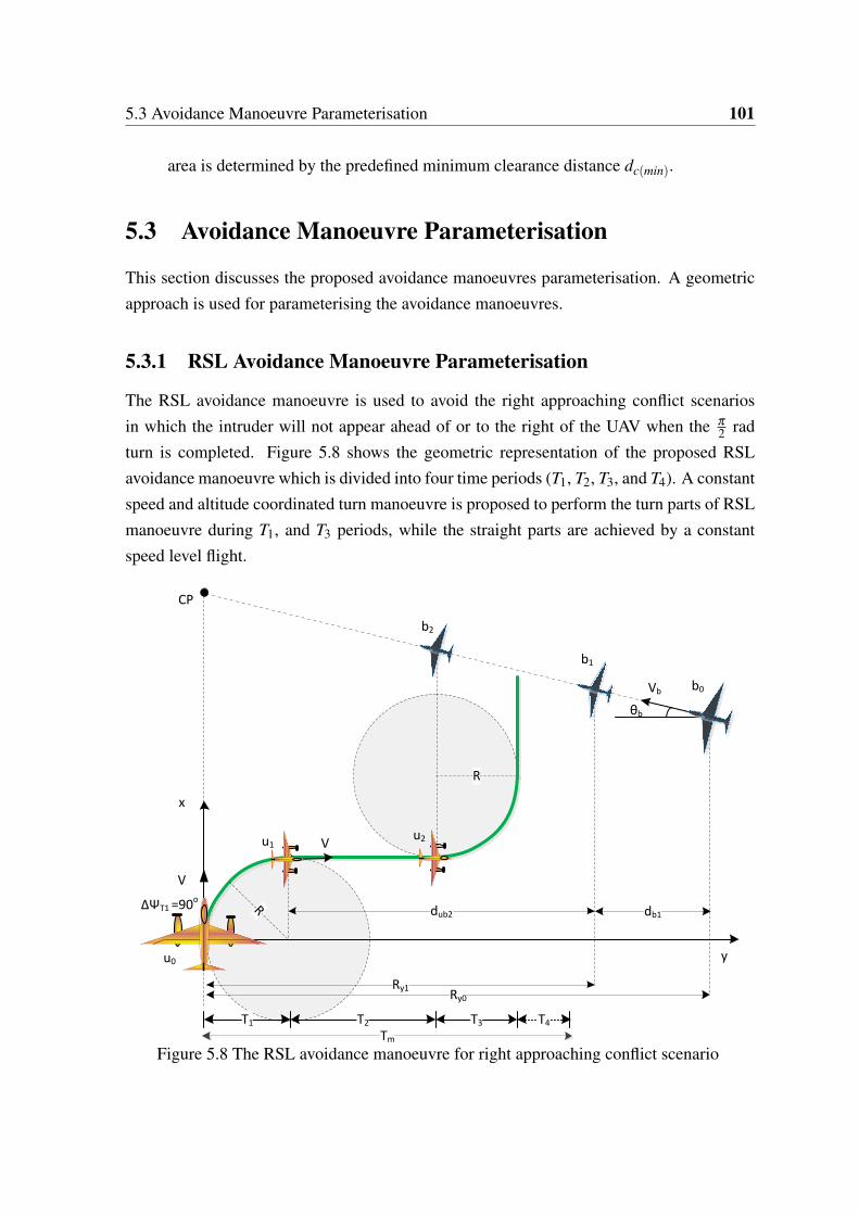
5.3 Avoidance Manoeuvre Parameterisation 101
area is determined by the predefined minimum clearance distance dc(min).
5.3 Avoidance Manoeuvre Parameterisation
This section discusses the proposed avoidance manoeuvres parameterisation. A geometricapproach is used for parameterising the avoidance manoeuvres.
5.3.1 RSL Avoidance Manoeuvre Parameterisation
The RSL avoidance manoeuvre is used to avoid the right approaching conflict scenariosin which the intruder will not appear ahead of or to the right of the UAV when the π
2 radturn is completed. Figure 5.8 shows the geometric representation of the proposed RSLavoidance manoeuvre which is divided into four time periods (T1, T2, T3, and T4). A constantspeed and altitude coordinated turn manoeuvre is proposed to perform the turn parts of RSLmanoeuvre during T1, and T3 periods, while the straight parts are achieved by a constantspeed level flight.
R
CP
ΔΨT1 =90o
T1 T2 T3
R
T4
θb
Vb
V
b1
b2
u1
Ry1
Tm
u0
db1
b0
u2V
Ry0
y
x
dub2
Figure 5.8 The RSL avoidance manoeuvre for right approaching conflict scenario
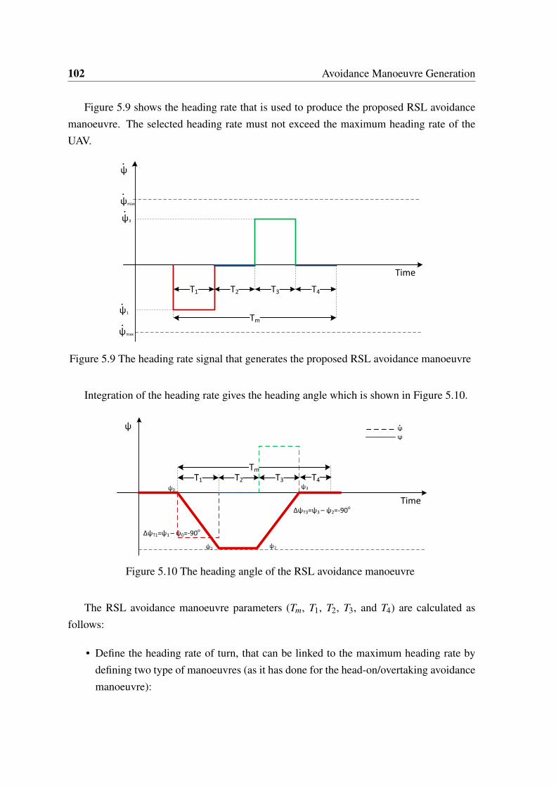
102 Avoidance Manoeuvre Generation
Figure 5.9 shows the heading rate that is used to produce the proposed RSL avoidancemanoeuvre. The selected heading rate must not exceed the maximum heading rate of theUAV.
ψ
ψmax
ψmax
Tm
T1 T2 T3
Time
ψ1
ψ3
T4
Figure 5.9 The heading rate signal that generates the proposed RSL avoidance manoeuvre
Integration of the heading rate gives the heading angle which is shown in Figure 5.10.
ψ
Tm
T1 T2 T3
Time
ψ0
ψ1 ψ2
ψ3
ΔψT1=ψ1 – ψ0=-90o
ΔψT3=ψ3 – ψ2=-90o
T4
Ψ
Ψ.
Figure 5.10 The heading angle of the RSL avoidance manoeuvre
The RSL avoidance manoeuvre parameters (Tm, T1, T2, T3, and T4) are calculated asfollows:
• Define the heading rate of turn, that can be linked to the maximum heading rate bydefining two type of manoeuvres (as it has done for the head-on/overtaking avoidancemanoeuvre):

5.3 Avoidance Manoeuvre Parameterisation 103
1. Average manoeuvre: ψ1 = [50%−75%]ψmax
2. Exaggerated manoeuvre: ψ1 = [75%−100%]ψmax
• Calculate the time period T1:
T1 =∆ψT1
ψ1=
π
2ψ1(5.18)
• Calculate the time period T2: At the beginning of time period T2 the UAV, and theintruder are at u1, and b1 positions respectively. They move to positions u2, and b2 atthe end of T2. Hence, the time period T2 is given by:
T2 =dub2
V +Vb cos(θb)(5.19)
where Vb is the intruder speed, θb is the angle between the intruder speed vector andthe y-axis, and dub2 is the projection of the distance between the UAV and the intruderat the end of the time period T1 on the y-axis:
dub2 = Ry0 − (R+db1) (5.20)
where Ry0 is the initial intruder range projection on the y-axis, R is the turn radiusgiven by (5.3), and db1 is the projection on the y-axis of the traveled distance by theintruder during the time period T1:
db1 =Vb cos(θb)T1 (5.21)
Unlike the avoidance manoeuvre for the head-on/overtaking conflict scenarios, theRSL avoidance manoeuvre calculation depends on the intruder speed and heading(during the time period T2).
• Calculate the time period T3: In order to make sure that the UAV heading angle at theend of time period T3 is the same as the UAV initial heading angle, the time period T3
is chosen to be equal to the time period T1, and ψ3 =−ψ1.
• Calculate the time period T4: T4 = Tm − (T1 +T2 +T3).

104 Avoidance Manoeuvre Generation
5.3.2 RS-LS Avoidance Manoeuvre Parameterisation
The time period T2 in the RSL avoidance manoeuvre calculation depends on the intruder’sinitial state (heading angle, and speed). The intruder’s speed and heading angle are sup-posed to be held during the conflict when the UAV is performing the avoidance manoeuvre(according to the rules of the air). However, mismatch between the actual intruder state andthe available one (measured by the on-board sensing unit, or provided by the ground station)should be taken into consideration. Also, using the available intruder’s initial state values tocalculate the whole avoidance manoeuvre is not sufficient if these values are changed duringthe avoidance manoeuvre performing. Therefore, updated values of the intruder’s state canbe useful to reduce the mismatch effects and to overcome the intruder’s state values changesproblem. Hence, the RS-LS avoidance manoeuvre, which is a modified version of RSLavoidance manoeuvre, is proposed to overcome the RSL drawbacks. The RS-LS avoidancemanoeuvre is divided into two parts: Right-Straight RS, then Left-Straight LS. While theRS part is initiated by the collision flag CF, the LS part is initiated by NF flag. The NF flagis proposed to be activated when the UAV is performing the avoidance manoeuvre, and theintruder is at the 9 o’clock position relative to the UAV. Figure 5.11 illustrates the sequenceof the RS-LS avoidance manoeuvre parts with the collision assessment flags (CF, NF, andRF), and shows the heading rate values during the time periods.
0
CF
T3
Tm1
T1 T2
T4
RF
Start the RS-LS avoidance manoeuvreStop the avoidance manoeuvre;Return to the global trajectory
0
Time
ψ1
. .ψ3
NF
Tm2
Start RS part
Start LS part
Figure 5.11 The RS-LS avoidance manoeuvre parts sequence
• Predefined time values Tm1, and Tm2 are given for manoeuvre parts RS, LS parts re-spectively. They should be selected to be large enough to perform the avoidancemanoeuvre.

5.3 Avoidance Manoeuvre Parameterisation 105
• The time periods T1, and T3 are calculated in the same manner as in the RSL avoidancemanoeuvre.
• While the time period T2 = Tm1 − T1 is interrupted by the NF flag, the time periodT4 = Tm2 −T3 is interrupted by the RF flag.
5.3.3 Circle Avoidance Manoeuvre Parameterisation
The RSL/RS-LS avoidance manoeuvres are not suitable for some right approaching conflictscenarios. For example, conflict scenario C that is discussed in Section 5.2.3 in which theposition of the intruder at the end of time period T1 is nearly at a head-on position withthe UAV. So instead of going straight, the proposed manoeuvre, is to make a full circlemanoeuvre. The circle avoidance manoeuvre is proposed for the right approaching conflictscenarios if the intruder will be at the head-on position, or at the right of the UAV whenit completes π
2 rad right turn. This will guarantee that the UAV is not going to cross theintruder flight path (this is one of the rules of the air requirements). Figure 5.12 gives ageometric representation of the circle avoidance manoeuvre.
CP
Tt
R c0
u1c1
c2
u2
u3
dc(min)
xmin
Vc
θc
x
yu0
Rx1
Rx0
dc1
Figure 5.12 The geometric representation of the proposed circle avoidance manoeuvre

106 Avoidance Manoeuvre Generation
The condition to perform the circle manoeuvre instead of the RSL/RS-LS avoidancemanoeuvre is:
Rx1 ≤ Xmin ⇒ Rx1 ≤ R+dc(min) (5.22)
where Rx1 is the intruder range projection on the x-axis, when it at the position c1 (theintruder ranges are measured from the reference frame origin at u0), R is the turn radius,and dc(min) is a predefined minimum clearance distance, measured from the UAV positionu1 (when it complete π
2 rad right turn). The intruder range projections Rx1 is given by:
Rx1 = Rx0 +dc1 (5.23)
where Rx0 is the intruder range projection on the x-axis when it is at the position c0, and dc1
is the projection of the intruder traveled distance from c0 to c1 given by:
dc1 =Tt
4Vc sin(θc) (5.24)
where Vc is the intruder speed, θc is the angle between the y-axis and the intruder speedvector as shown in Figure 5.12, and Tt is a full circle turn time given by (5.26). Then thecircle avoidance manoeuvre condition can be written:
Rx0 ≤ R+dc(min)−Tt
4Vc sin(θc) (5.25)
It can be noted that this avoidance manoeuvre is simply a circle path with a constant speedand altitude (coordinated turn). The circle radius is controlled by the selected heading rateψ shown in Figure 5.13, and the UAV speed V . The relationship of circle radius is giveby (5.3). The UAV heading angle is shown in Figure 5.14. As can be seen in Figures 5.13and 5.14 the manoeuvre is divided into two periods:
• The circle turn time period Tt :
Tt =∆ψTt
ψ1=
2π
ψ1(5.26)
where ψ1 is the selected avoidance heading rate
• The time period T4: As the manoeuvre time Tm is predefined, so T4 = Tm −Tt

5.3 Avoidance Manoeuvre Parameterisation 107
ψ
ψmax
ψmaxTm
Time
ψ1
Tt T4
Figure 5.13 Heading rate for the circle avoidance manoeuvre
ψ
Tm
Tt
Time
ψ0
ψ1
ΔψT1=ψ1 – ψ0=-360o
T4
Figure 5.14 Heading angle for the circle avoidance manoeuvre
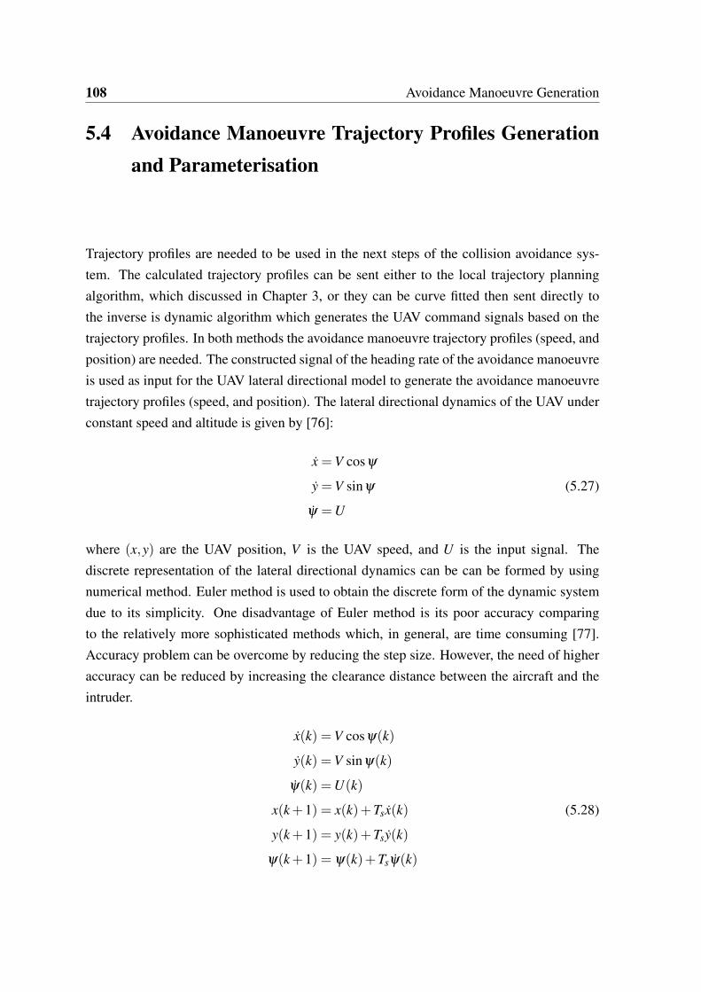
108 Avoidance Manoeuvre Generation
5.4 Avoidance Manoeuvre Trajectory Profiles Generationand Parameterisation
Trajectory profiles are needed to be used in the next steps of the collision avoidance sys-tem. The calculated trajectory profiles can be sent either to the local trajectory planningalgorithm, which discussed in Chapter 3, or they can be curve fitted then sent directly tothe inverse is dynamic algorithm which generates the UAV command signals based on thetrajectory profiles. In both methods the avoidance manoeuvre trajectory profiles (speed, andposition) are needed. The constructed signal of the heading rate of the avoidance manoeuvreis used as input for the UAV lateral directional model to generate the avoidance manoeuvretrajectory profiles (speed, and position). The lateral directional dynamics of the UAV underconstant speed and altitude is given by [76]:
x =V cosψ
y =V sinψ (5.27)
ψ =U
where (x,y) are the UAV position, V is the UAV speed, and U is the input signal. Thediscrete representation of the lateral directional dynamics can be can be formed by usingnumerical method. Euler method is used to obtain the discrete form of the dynamic systemdue to its simplicity. One disadvantage of Euler method is its poor accuracy comparingto the relatively more sophisticated methods which, in general, are time consuming [77].Accuracy problem can be overcome by reducing the step size. However, the need of higheraccuracy can be reduced by increasing the clearance distance between the aircraft and theintruder.
x(k) =V cosψ(k)
y(k) =V sinψ(k)
ψ(k) =U(k)
x(k+1) = x(k)+Tsx(k) (5.28)
y(k+1) = y(k)+Tsy(k)
ψ(k+1) = ψ(k)+Tsψ(k)

5.4 Avoidance Manoeuvre Trajectory Profiles Generation and Parameterisation 109
where Ts is the sampling time, and k = 0,1, . . . ,n is the discrete steps. The relationshipbetween the time manoeuvre and sampling time is n = Tm
Ts. Hence, the constructed heading
rate signal is discretised then used to generate the discrete speed and position profiles of theproposed avoidance manoeuvre.
ψ = [ψ(0), ψ(1), . . . , ψ(n−1), ψ(n)] (5.29)
Figure 5.15 shows the flowchart of the avoidance manoeuvre trajectory profiles calculation.
No
Start
End
Yes
Figure 5.15 Flowchart of discrete trajectory profiles calculation
The generated trajectory profiles (position, and speed) can then be curve fitted to cal-
110 Avoidance Manoeuvre Generation
culate all the trajectory profiles (position, and speed, acceleration, and jerk) which can beused by the inverse dynamic algorithm to generate the command signals for the UAV controlsystem. Alternatively it can be used as a global trajectory for the LTP algorithm.
5.4.1 Avoidance Manoeuvre Trajectory Profiles Curve Fitting
The inverse dynamic algorithm that generates the command signal for the UAV dependson the trajectory profiles (position, speed, acceleration, and rate of acceleration) in the 3Dreference frame. However, the discretized lateral directional model of the UAV 5.28 with theconstructed heading rate signal as input generates only the speed and position profiles in the2D reference frame. Thus, a 6th order Bezier curve is used to curve fit the generated speedprofiles. Then the Bezier curve coefficients are used to generate the avoidance manoeuvretrajectory profiles in the 3D reference frame. The curve fitting algorithm uses the leastsquares curve fitting technique which is discussed in Appendix A. The coefficients of theBezier curve that fits the speed profiles are calculated as:
Cx = Blsx
Cy = Blsy (5.30)
Cz = Blsz = 0
where C = [c0,c1, . . . ,c6] are the Bezier curve coefficients, Bls is the curve-fit matrix whichis calculated off-line using the Bezier basis function matrices B (see Appendix A):
Bls = (BT B)−1BT (5.31)
The coefficients of the Beizer curve are used to calculate the trajectory profiles (position,speed, acceleration, and rate of acceleration) in the 3D reference frame. The curve fittedspeed profiles in forward (u), lateral (v), and vertical (w) axes are written:
u(τ) = cx0B0(τ)+ cx
1B1(τ)+ cx2B2(τ)+ · · ·+ cx
6B6(τ)
v(τ) = cy0B0(τ)+ cy
1B1(τ)+ cy2B2(τ)+ · · ·+ cy
6B6(τ) (5.32)
w(τ) = cz0B0(τ)+ cz
1B1(τ)+ cz2B2(τ)+ · · ·+ cz
6B6(τ)
However, in horizontal manoeuvres the vertical speed (w(τ) = 0), hence:
czi = 0; i = 0,1, · · · ,6 (5.33)
5.4 Avoidance Manoeuvre Trajectory Profiles Generation and Parameterisation 111
The relationship between the parameter τ and the avoidance manoeuvre time (Tm) can beused to represent the time t = Tm.τ . Therefore, the acceleration and the jerk profiles aregiven by:
dudt
=1
Tm
(cx
0dB0(τ)
dτ+ · · ·+ cx
6dB6(τ)
dτ
)(5.34)
andd2udt2 =
1T 2
m
(cx
0d2B0(τ)
dτ2 + · · ·+ cx6
d2B6(τ)
dτ2
)(5.35)
The acceleration and the jerk profiles for the lateral axis can be calculated in a similar way.The acceleration and jerk profiles for the vertical axis are zeros. The position profile isdriven by integration of the basis functions with respect to time t.
Binti =
∫ Tm
0Bi(t)dt; i = 0,1, . . . ,6 (5.36)
Hence, the trajectory profiles calculation is reduced to simple matrix multiplication:
u =CxTB, u =
1Tm
CxTB′,
u =1
T 2m
CxTB′′, x = x0 +CxT
Bint(5.37)
v =CyTB, v =
1Tm
CyTB′,
v =1
T 2m
CyTB′′, y = y0 +CyT
Bint(5.38)
w =CzTB, w =
1Tm
CzTB′,
w =1
T 2m
CzTB′′, z = z0 +CzT
Bint(5.39)
where:B: Is the discretised basis function matrix given by:
B =
B0(τ1) B0(τ2) · · · B0(τn)
B1(τ1) B1(τ2) · · · B1(τn)...
... · · · ...B6(τ1) B6(τ2) · · · B6(τn)
(5.40)
112 Avoidance Manoeuvre Generation
B′, B′′: Are the discretised basis function derivatives matrices. More about these matricescan be found in Chapter 3.CuT
, CvT, CwT
: Are the vectors of coefficients for forward, lateral, and vertical axis:
CxT=[cx
0 cx1 · · · cx
6
]CyT
=[cy
0 cy1 · · · cy
6
]CzT
=[cz
0 cz1 · · · cz
6
] (5.41)
The generated trajectory profiles are then passed directly to the inverse dynamics to gen-erate the control commands for the UAV control system. Although this method has someadvantages, such as, simplicity, and reduction the CAS algorithm computational time, it hassome drawbacks:
• The curve fitting process accuracy depends on the selected manoeuvre time Tm, andthe number of discretising steps n. So using long manoeuvre time reduces the fittingaccuracy.
• The trajectory profiles are generated without considering the UAV dynamic con-straints, which may lead to controller saturation in the UAV control layer.
• Passing the generated trajectory profiles directly to the inverse dynamics, means thatthe UAV will not be able to avoid any sudden collision with any pop-up obstaclesthat may happen during the avoidance manoeuvre execution. However, if the UAV isflying in a well known environment and the possibility of having a pop-up obstacle iscanceled this method can be used, but it needs more development to include the UAVdynamics constraints in the curve fitting process.
The other proposed method uses the generated trajectory profiles (position, and speed thatgenerated by the UAV lateral directional model Figure 5.15) as a global trajectory for thelocal trajectory planning (LTP) which uses the receding horizon technique to generate thetrajectory profiles (the LTP method is discussed in Chapter 2). Although the LTP algorithmavoids the curve-fitting method drawbacks because it curve fits a specific portion of theavoidance manoeuvre trajectory profiles at each step of time horizon and also takes theUAV and obstacle constraints into consideration, its computational time is higher. In thisthesis this method is used. The two methods are shown in the flowchart in Figure 5.16 whichgives the head-on/overtaking avoidance manoeuvre as an example.

5.4 Avoidance Manoeuvre Trajectory Profiles Generation and Parameterisation 113
Start
Exaggerated/average (Right/Left) manoeuvre;
Tm; dc; Ømax; V; ΔΨT1
Generate speed and position profiles by applying the calculated heading rate on UAV lateral directional model
Method selection
curve fit the generated speed profiles to calculate the Bezier curve coefficients
Calculate all profiles (position, speed, acceleration, and rate of acceleration)
Send the generated speed and position profiles to (LTP) algorithm
Send the trajectory profiles to the inverse dynamics algorithm which generates the command signals
End
Generate the heading rate signal ψ.
Calculate time periodsT1; T2; T3;T4; and heading rateψ1
Figure 5.16 CAS Flowchart

114 Avoidance Manoeuvre Generation
5.5 Simulation Results
This section discusses the simulation results for some avoidance manoeuvre scenarios.MATLAB/Simulink are used to test the proposed avoidance manoeuvres for different colli-sion scenarios. Figure 5.17 shows the block diagram that is used to generate the simulationresults. The UAV with the controllers are modeled by the point-mass model, and it is as-sumed that the UAV is tracking the generated command signals exactly. The switch andthe dashed link that are shown in the block diagram represent the method for generating thecommand signals by passing the trajectory profiles, that are generated by the curve fittingalgorithm, directly to the inverse dynamic.
Inverse
DynamicsAircraft Model
Local Trajectory
Planner
Trajectory
profiles
Conflict
Scenario
Avoidance
Manoeuvre
Generator
Control
System
Actual values
Demanded
values
Generated
values
Vehicle state
Figure 5.17 Block diagram for CAS simulation
5.5.1 Head-on Scenario Simulation Results
Figure 5.18 shows a head-on conflict scenario where the initial state of the UAV and theintruder are:
1. UAV initial state:
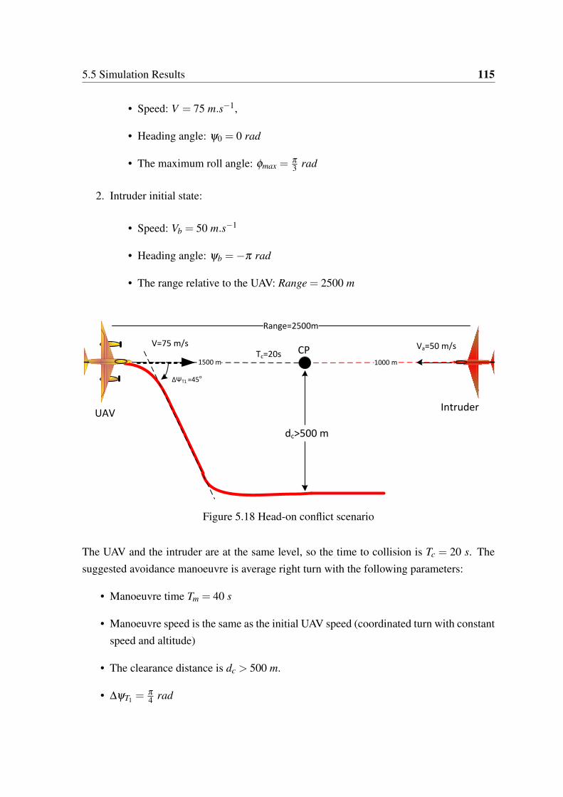
5.5 Simulation Results 115
• Speed: V = 75 m.s−1,
• Heading angle: ψ0 = 0 rad
• The maximum roll angle: φmax =π
3 rad
2. Intruder initial state:
• Speed: Vb = 50 m.s−1
• Heading angle: ψb =−π rad
• The range relative to the UAV: Range = 2500 m
1500 m 1000 m
CP
ΔΨT1 =45o
dc>500 m
V=75 m/s Va=50 m/s
Range=2500m
Tc=20s
UAVIntruder
Figure 5.18 Head-on conflict scenario
The UAV and the intruder are at the same level, so the time to collision is Tc = 20 s. Thesuggested avoidance manoeuvre is average right turn with the following parameters:
• Manoeuvre time Tm = 40 s
• Manoeuvre speed is the same as the initial UAV speed (coordinated turn with constantspeed and altitude)
• The clearance distance is dc > 500 m.
• ∆ψT1 =π
4 rad
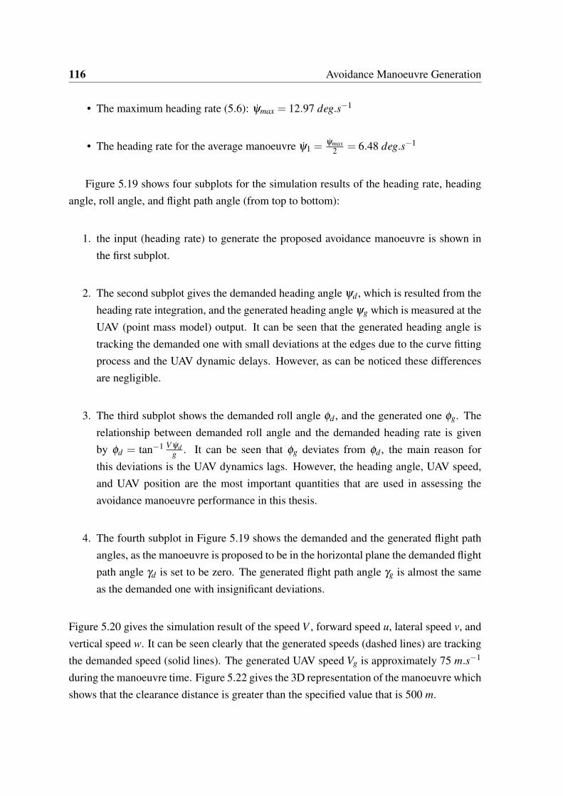
116 Avoidance Manoeuvre Generation
• The maximum heading rate (5.6): ψmax = 12.97 deg.s−1
• The heading rate for the average manoeuvre ψ1 =ψmax
2 = 6.48 deg.s−1
Figure 5.19 shows four subplots for the simulation results of the heading rate, headingangle, roll angle, and flight path angle (from top to bottom):
1. the input (heading rate) to generate the proposed avoidance manoeuvre is shown inthe first subplot.
2. The second subplot gives the demanded heading angle ψd , which is resulted from theheading rate integration, and the generated heading angle ψg which is measured at theUAV (point mass model) output. It can be seen that the generated heading angle istracking the demanded one with small deviations at the edges due to the curve fittingprocess and the UAV dynamic delays. However, as can be noticed these differencesare negligible.
3. The third subplot shows the demanded roll angle φd , and the generated one φg. Therelationship between demanded roll angle and the demanded heading rate is givenby φd = tan−1 V ψd
g . It can be seen that φg deviates from φd , the main reason forthis deviations is the UAV dynamics lags. However, the heading angle, UAV speed,and UAV position are the most important quantities that are used in assessing theavoidance manoeuvre performance in this thesis.
4. The fourth subplot in Figure 5.19 shows the demanded and the generated flight pathangles, as the manoeuvre is proposed to be in the horizontal plane the demanded flightpath angle γd is set to be zero. The generated flight path angle γg is almost the sameas the demanded one with insignificant deviations.
Figure 5.20 gives the simulation result of the speed V , forward speed u, lateral speed v, andvertical speed w. It can be seen clearly that the generated speeds (dashed lines) are trackingthe demanded speed (solid lines). The generated UAV speed Vg is approximately 75 m.s−1
during the manoeuvre time. Figure 5.22 gives the 3D representation of the manoeuvre whichshows that the clearance distance is greater than the specified value that is 500 m.
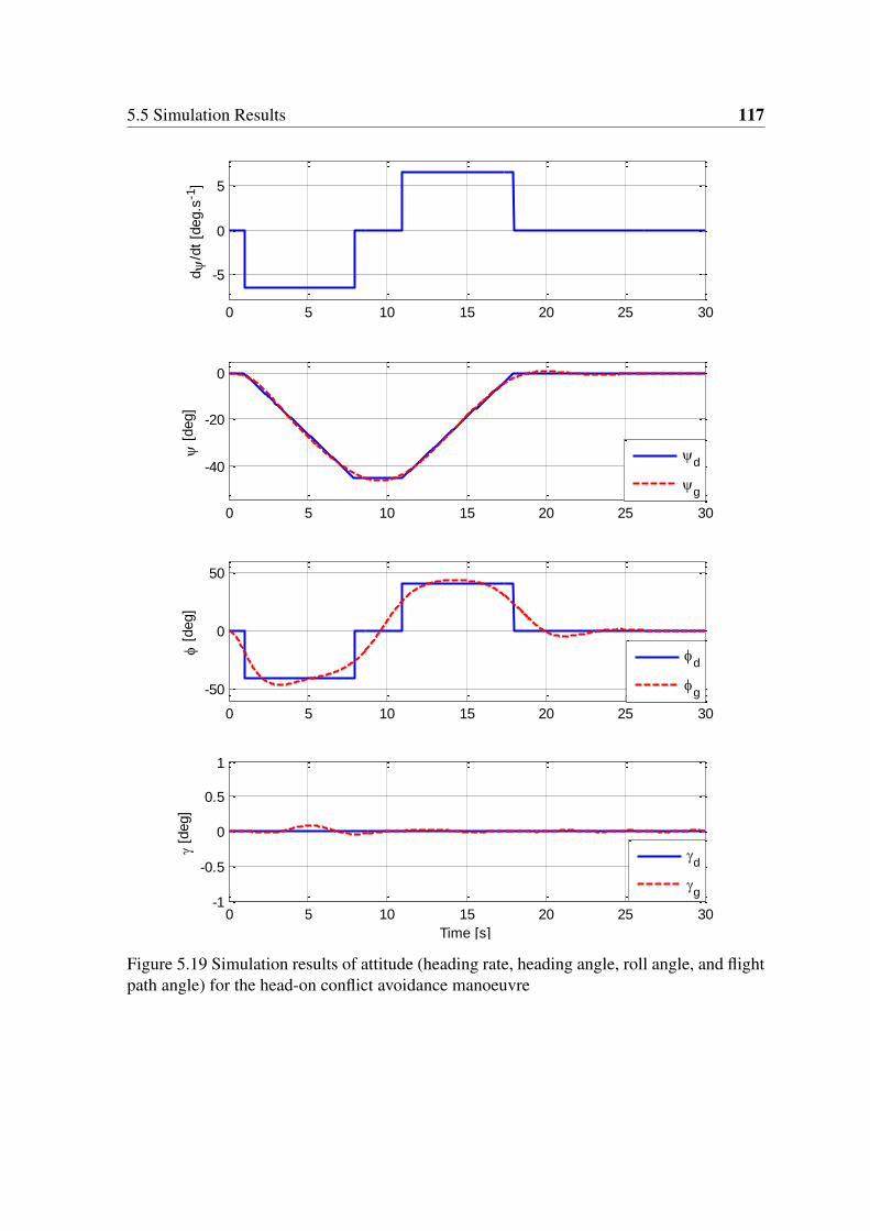
5.5 Simulation Results 117
0 5 10 15 20 25 30
-5
0
5d
/dt
[deg.s
-1]
0 5 10 15 20 25 30
-40
-20
0
[
deg]
d
g
0 5 10 15 20 25 30
-50
0
50
[
deg]
d
g
0 5 10 15 20 25 30-1
-0.5
0
0.5
1
[d
eg]
Time [s]
d
g
Figure 5.19 Simulation results of attitude (heading rate, heading angle, roll angle, and flightpath angle) for the head-on conflict avoidance manoeuvre
118 Avoidance Manoeuvre Generation
0 5 10 15 20 25 3072
74
76
78U
AV
speed [
m.s
-1]
Vd
Vg
0 5 10 15 20 25 30
50
60
70
80
Forw
ard
speed [
m.s
-1]
ud
ug
0 5 10 15 20 25 30
-40
-20
0
Late
ral speed [
m.s
-1]
vd
vg
0 5 10 15 20 25 30-1
-0.5
0
0.5
1
Time [sec]
Vert
ical speed [
m.s
-1]
wd
wg
Figure 5.20 Simulation results of speeds (V , u, v , and w) for the head-on conflict avoidancemanoeuvre
Figure 5.21 shows the normal load factor and 1cos(φ) during the avoidance manoeuvre. It
can be seen that the load factor meets the requirements given in CS-23 document [69] and

5.5 Simulation Results 119
equals to 1cos(φ) hence it satisfies 5.8. This is another factor, in addition to the speed and
altitude results, shows that coordinated turn is performed smoothly.
0 5 10 15 20 25 300.8
1
1.2
1.4
Time [sec]
Load factor
1/cos()
Figure 5.21 Load factor during the avoidance manoeuvre
-500
0
500
1000
1500
2000
2500
3000
-1500
-1000
-500
0
500
800
900
1000
1100
1200
X [m]
X: 2077
Y: -553.7
Z: 1000X: 1402
Y: -553.1
Z: 1000
X: 2500
Y: 0
Z: 1000
Y [m]
X: 0
Y: 0
Z: 1000
X: 1450
Y: 1.286e-013
Z: 1000X: 1000
Y: 1.837e-013
Z: 1000
Z [
m]
Demanded trajectory
Generated trajectory
Intruder trajectory
UAV initial position
Intruder initial position
UAV psosition at t=Tc
Intruder position at t=Tc
UAV psosition at t=30 sec
Intruder position at t=30 sec
Figure 5.22 3D view of the UAV trajectory for the head-on conflict avoidance manoeuvre

120 Avoidance Manoeuvre Generation
5.5.2 Right Approaching Conflict Scenario Simulation Results (RSLmanoeuvre)
Figure 5.23 shows a right approaching scenario used to test the RSL avoidance manoeuvre.The initial state for the UAV and the intruder are:
1. UAV initial state:
• Speed: V = 75 m.s−1,
• Heading angle: ψ0 = 0 rad
• Maximum roll angle: φmax =π
3 rad
2. Intruder initial state:
• Speed: Vb = 75 m.s−1
• Heading angle: ψb =π
3 rad, that means θb =π
6 rad
• Range relative to the UAV: Ry0 = 1500 m
• Time to collision: Tc = 20 s
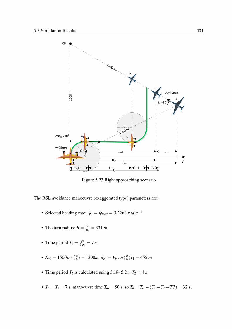
5.5 Simulation Results 121
R
1500 m
15
00
m
CP
ΔΨT1 =90o
T1 T2 T3
R
T4
1500 m
θb =30o
Vb=75m/s
V=75m/sxb2
b1
b2
u1
dub1
Tm
Ry0y
db1
b0
u2
Ry1
Figure 5.23 Right approaching scenario
The RSL avoidance manoeuvre (exaggerated type) parameters are:
• Selected heading rate: ψ1 = ψmax = 0.2263 rad.s−1
• The turn radius: R = Vψ1
= 331 m
• Time period T1 =pi
2ψ1= 7 s
• Ry0 = 1500cos(π
6 ) = 1300m, db1 =Vb cos(π
6 )T1 = 455 m
• Time period T2 is calculated using 5.19- 5.21: T2 = 4 s
• T3 = T1 = 7 s, manoeuvre time Tm = 50 s, so T4 = Tm − (T1 +T2 +T 3) = 32 s,

122 Avoidance Manoeuvre Generation
0 5 10 15 20 25 30
-10
0
10
d
/dt
[deg.s
-1]
0 5 10 15 20 25 30
-100
-50
0
[
deg]
d
g
0 5 10 15 20 25 30
-50
0
50
[
deg]
d
g
0 5 10 15 20 25 30-5
0
5
[d
eg]
Time [s]
d
g
Figure 5.24 Simulation results of attitude (heading rate, heading angle, roll angle, and flightpath angle) for the RSL avoidance manoeuvre
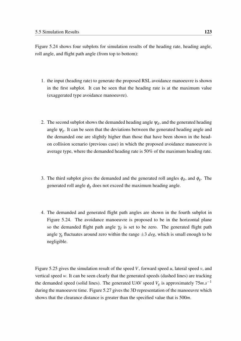
5.5 Simulation Results 123
Figure 5.24 shows four subplots for simulation results of the heading rate, heading angle,roll angle, and flight path angle (from top to bottom):
1. the input (heading rate) to generate the proposed RSL avoidance manoeuvre is shownin the first subplot. It can be seen that the heading rate is at the maximum value(exaggerated type avoidance manoeuvre).
2. The second subplot shows the demanded heading angle ψd , and the generated headingangle ψg. It can be seen that the deviations between the generated heading angle andthe demanded one are slightly higher than those that have been shown in the head-on collision scenario (previous case) in which the proposed avoidance manoeuvre isaverage type, where the demanded heading rate is 50% of the maximum heading rate.
3. The third subplot gives the demanded and the generated roll angles φd , and φg. Thegenerated roll angle φg does not exceed the maximum heading angle.
4. The demanded and generated flight path angles are shown in the fourth subplot inFigure 5.24. The avoidance manoeuvre is proposed to be in the horizontal planeso the demanded flight path angle γd is set to be zero. The generated flight pathangle γg fluctuates around zero within the range ±3 deg, which is small enough to benegligible.
Figure 5.25 gives the simulation result of the speed V , forward speed u, lateral speed v, andvertical speed w. It can be seen clearly that the generated speeds (dashed lines) are trackingthe demanded speed (solid lines). The generated UAV speed Vg is approximately 75m.s−1
during the manoeuvre time. Figure 5.27 gives the 3D representation of the manoeuvre whichshows that the clearance distance is greater than the specified value that is 500m.

124 Avoidance Manoeuvre Generation
0 5 10 15 20 25 3050
60
70
80
90
100U
AV
speed [
m.s
-1]
Vd
Vg
0 5 10 15 20 25 30
0
20
40
60
80
Forw
ard
speed [
m.s
-1]
ud
ug
0 5 10 15 20 25 30-80
-60
-40
-20
0
Late
ral speed [
m.s
-1]
vd
vg
0 5 10 15 20 25 30-5
0
5
Time [sec]
Vert
ical speed [
m.s
-1]
wd
wg
Figure 5.25 Simulation results of speeds (V , u, v , and w) for the RSL avoidance manoeuvre
Figure 5.26 shows the normal load factor and 1cos(φ) simulation results. Unlike the head-
on conflict scenario, that is discussed previously, there is mismatch between n and 1cos(φ)
due to the higher value of the heading rate (command) of the exaggerated type avoidancemanoeuvre. However, the normal load factor still meet the criteria that given in CS-23 [69].

5.5 Simulation Results 125
0 5 10 15 20 25 300
0.5
1
1.5
2
2.5
3
Time [sec]
Load factor
1/cos()
Figure 5.26 Load factor during the avoidance manoeuvre
-500
0
500
1000
1500
2000
2500
3000
-1500
-1000
-500
0
500
800
900
1000
1100
1200
X [m]
X: 750
Y: -1299
Z: 1000
X: 1200
Y: -519.6
Z: 1000
X: 403.1
Y: -616.7
Z: 1002
Y [m]
X: 0
Y: 0
Z: 1000
Z [
m]
Demanded trajectory
Generated trajectory
Intruder trajectory
UAV initial position
Intruder initial position
UAV psosition at t=Tc
Intruder position at t=Tc
UAV psosition at the end of T2 period
Intruder position at the end of T2 period
UAV psosition at t=30 sec
Intruder position at t=30 sec
Figure 5.27 3D view of the UAV trajectory for the RSL avoidance manoeuvre

126 Avoidance Manoeuvre Generation
5.5.3 Right Approaching conflict Scenario Simulation Results (CircleManoeuvre)
Figure 5.28 shows a right approaching scenario used to test the circle avoidance manoeuvre.The initial state for the UAV and the intruder are:
1. UAV initial state:
• Speed: V = 60 m.s−1,
• Heading angle: ψ0 = 0 rad
• Maximum roll angle: φmax =π
3 rad
2. Intruder initial state:
• Speed: Vb = 75 m.s−1
• Heading angle: ψc = 0.89 rad, that means θc = 0.68 rad
• Range relative to the UAV: Range = 1500 m
• Time to collision: Tc = 25 s
The circle avoidance manoeuvre (exaggerated type) parameters are:
• Selected heading rate: ψ1 = 0.8ψmax = 0.2263 rad.s−1
• Turn radius: R = Vψ1
= 265 m
• Time period Tt =2π
ψ1= 27.76 s
• Rx0 =−312 m, dc1 =Vc cos(θc)Tt4 = 455 m
• T4 = Tm − (Tt) = 11.24 s,
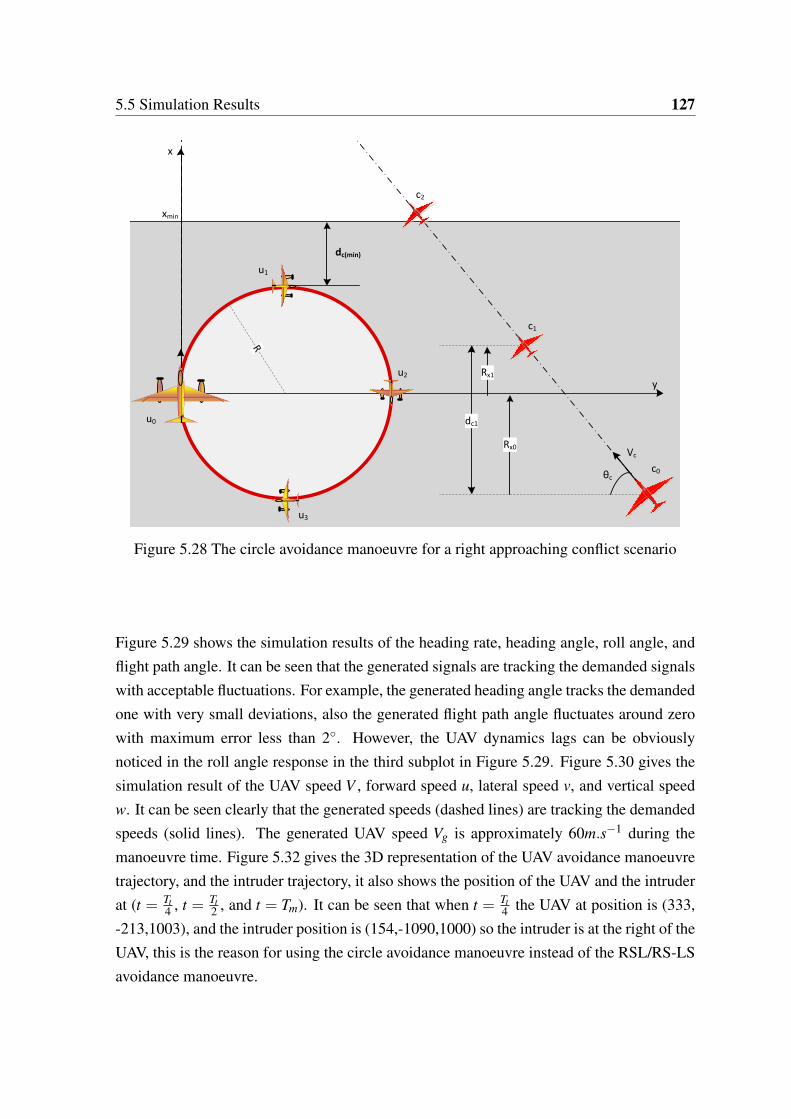
5.5 Simulation Results 127
R
Rx1
c0
u1
c1
c2
u2
u3
dc(min)
xmin
Vc
θc
x
y
u0
Rx0
dc1
Figure 5.28 The circle avoidance manoeuvre for a right approaching conflict scenario
Figure 5.29 shows the simulation results of the heading rate, heading angle, roll angle, andflight path angle. It can be seen that the generated signals are tracking the demanded signalswith acceptable fluctuations. For example, the generated heading angle tracks the demandedone with very small deviations, also the generated flight path angle fluctuates around zerowith maximum error less than 2◦. However, the UAV dynamics lags can be obviouslynoticed in the roll angle response in the third subplot in Figure 5.29. Figure 5.30 gives thesimulation result of the UAV speed V , forward speed u, lateral speed v, and vertical speedw. It can be seen clearly that the generated speeds (dashed lines) are tracking the demandedspeeds (solid lines). The generated UAV speed Vg is approximately 60m.s−1 during themanoeuvre time. Figure 5.32 gives the 3D representation of the UAV avoidance manoeuvretrajectory, and the intruder trajectory, it also shows the position of the UAV and the intruderat (t = Tt
4 , t = Tt2 , and t = Tm). It can be seen that when t = Tt
4 the UAV at position is (333,-213,1003), and the intruder position is (154,-1090,1000) so the intruder is at the right of theUAV, this is the reason for using the circle avoidance manoeuvre instead of the RSL/RS-LSavoidance manoeuvre.

128 Avoidance Manoeuvre Generation
0 5 10 15 20 25 30 35 40
-15
-10
-5
0
5d
/dt
[deg.s
-1]
0 5 10 15 20 25 30 35 40
-400
-300
-200
-100
0
[
deg]
d
g
0 5 10 15 20 25 30 35 40
-50
0
50
[
deg]
d
g
0 5 10 15 20 25 30 35 40-5
0
5
[d
eg]
Time [s]
d
g
Figure 5.29 Simulation results of attitude (heading rate, heading angle, roll angle, and flightpath angle) for the circle avoidance manoeuvre
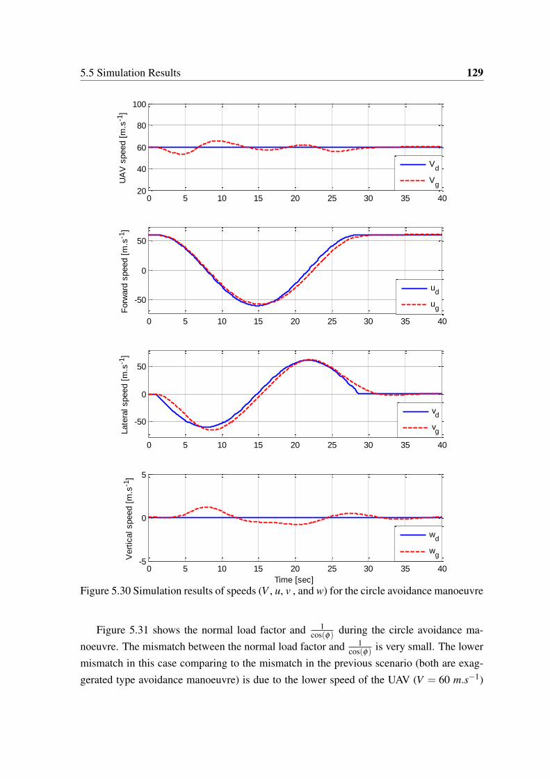
5.5 Simulation Results 129
0 5 10 15 20 25 30 35 4020
40
60
80
100
UA
V s
peed [
m.s
-1]
Vd
Vg
0 5 10 15 20 25 30 35 40
-50
0
50
Forw
ard
speed [
m.s
-1]
ud
ug
0 5 10 15 20 25 30 35 40
-50
0
50
Late
ral speed [
m.s
-1]
vd
vg
0 5 10 15 20 25 30 35 40-5
0
5
Time [sec]
Vert
ical speed [
m.s
-1]
wd
wg
Figure 5.30 Simulation results of speeds (V , u, v , and w) for the circle avoidance manoeuvre
Figure 5.31 shows the normal load factor and 1cos(φ) during the circle avoidance ma-
noeuvre. The mismatch between the normal load factor and 1cos(φ) is very small. The lower
mismatch in this case comparing to the mismatch in the previous scenario (both are exag-gerated type avoidance manoeuvre) is due to the lower speed of the UAV (V = 60 m.s−1)

130 Avoidance Manoeuvre Generation
than the speed in the previous case (V = 75 m.s−1).
0 5 10 15 20 25 30 35 400
0.5
1
1.5
2
2.5
3
Time [sec]
Load factor
1/cos()
Figure 5.31 Load factor during the avoidance manoeuvre
-500
0
500
1000
1500
2000
-1400-1200
-1000-800
-600-400
-2000
200400
600
800
900
1000
1100
1200
X [m]
X: -311.9
Y: -1467
Z: 1000
X: 154.1
Y: -1090
Z: 1000
Y [m]
X: 333
Y: -213.9
Z: 1003
X: 0
Y: 0
Z: 1000
Z [
m]
Demanded trajectory
Generated trajectory
Intruder trajectory
UAV initial position
Intruder initial position
UAV psosition at t=Tt/4
Intruder position at t=Tt/4
UAV psosition at t=Tt/2
Intruder position at t=Tt/2
UAV psosition at t=Tm
Intruder position at t=Tm
Figure 5.32 3D view of the UAV trajectory for the circle avoidance manoeuvre

5.6 Summary 131
5.6 Summary
This chapter discusses the avoidance manoeuvres generating process for different conflictscenarios in which the UAV should change direction (right/left turn) in horizontal plane.Two conflict scenarios are discussed, namely head-on, and right approaching. The rules ofthe air give general instructions for avoiding different conflict scenarios, but there are no spe-cific procedures for performing the avoidance manoeuvres. Hence, the proposed avoidancemanoeuvres that are presented in this chapter are selected based on a pilot’s suggestions. Ageometric approach is used to parameterize the proposed avoidance manoeuvres.


Chapter 6
Pilot Behaviour-Based CollisionAvoidance Manoeuvre Generation
6.1 Introduction
This chapter shows how pilot experience can be used to develop a collision avoidance ma-noeuvre generation process for a UAV. Although the avoidance manoeuvres proposed inChapter 5 are intended to be similar to the manoeuvres that are generated by pilots inmanned aircraft, they are predetermined manoeuvres. For example, at a specific value ofthe UAV speed and bank angle the avoidance manoeuvres will be the same for differentvalues of the time to collision. This is not the case in the manned aircraft, where the reac-tion of the pilot differs from one scenario to another. Consequently the produced avoidancemanoeuvres are not predetermined. Hence, a further development is proposed to link theavoidance manoeuvre’s parameters with the conflict scenario’s parameters. Thus, the gener-ated avoidance manoeuvre changes dynamically based on the conflict scenario in a similarmanner that the manned aircraft does. As a result, the UAV behaviour during the conflictbecomes more similar to the manned aircraft behaviour.
The proposal in this chapter is to augment the pilot’s experiences to the avoidance ma-noeuvre generating process. In a manned aircraft the pilot uses his/her experience to initiatethe suitable manoeuvre to avoid the conflict. Fuzzy logic technique is proposed to modelthe pilot actions in generating the avoidance manoeuvre for different conflict scenarios.
In this thesis the protocol for achieving the turn for the avoidance manoeuvre is obtainedfrom experience of a single pilot (See Appendix B) . The pilot in collision avoidance case

134 Pilot Behaviour-Based Collision Avoidance Manoeuvre Generation
initiates the turn by considering the time to collision Tc and the aircraft speed (V ) to inferthe amount of roll rate φ to bank the aircraft at a predetermined bank angle φ , and changethe aircraft heading angle by a predetermined value ∆ψ . The pilot experience is used togenerate the roll rate by using the fuzzy logic technique. Different head-on conflict scenar-ios are used to test the proposed algorithm by using MATLAB/Simulink. Simulation resultsare included and discussed.
It is important to mention that the pilot behaviour information during the collision avoid-ance, which is presented in this chapter, is based on a single pilot experience. Extractingthe pilot experience is achieved by extended interviews and a problem discussion with apilot at the National Flying Laboratory Centre, Cranfield University. Pilot behaviour differsfrom pilot to another according their experience, type of the aircraft, and the environmentthat they are flying in. A further development for this method can be achieved by involvingmore pilots with different experiences.
6.2 Fuzzy Logic Controller Structure
Since it was introduced by Zadeh in 1965, Fuzzy Logic (FL) has become a successful tech-nique for developing complex control systems [78]. Fuzzy logic techniques have been usedin a practical control systems successfully since the early 1970s, when the British engineerEbrahim Mamdani developed an automated control system for a steam engine using theexpertise of a human operator [79]. Commenting on his work, Mamdani wrote [80]:
The essence of this work is simply that if an experienced operator can provide
the protocol for achieving such a control in qualitative linguistic terms, then
fuzzy logic can be used to successfully implement this strategy.
It is appropriate to use fuzzy logic when [81]:
• The system has one or more continuous control variables,
• The mathematical model of the process does not exist, or it is very difficult to encode,or is very complex to be evaluated fast enough for real time operation, or involves toomuch memory on the designated chip architecture.
• High ambient noise levels must be dealt with or it is important to use inexpensivesensors and/or a low precision microcontroller.
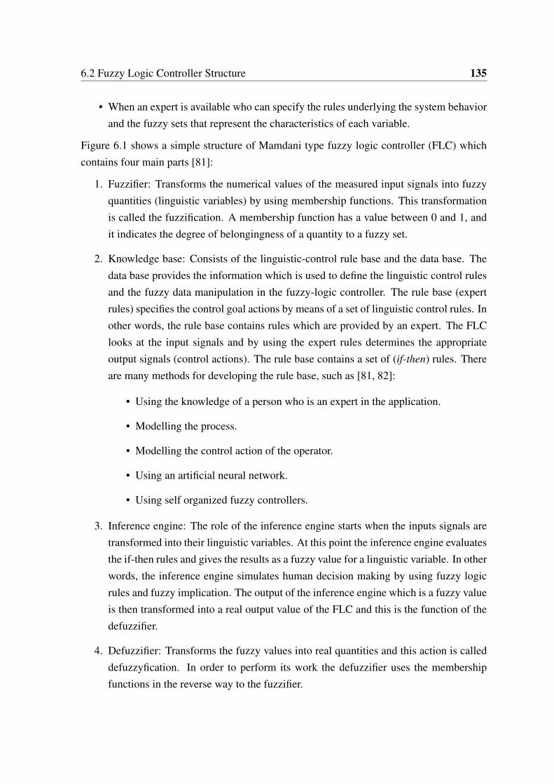
6.2 Fuzzy Logic Controller Structure 135
• When an expert is available who can specify the rules underlying the system behaviorand the fuzzy sets that represent the characteristics of each variable.
Figure 6.1 shows a simple structure of Mamdani type fuzzy logic controller (FLC) whichcontains four main parts [81]:
1. Fuzzifier: Transforms the numerical values of the measured input signals into fuzzyquantities (linguistic variables) by using membership functions. This transformationis called the fuzzification. A membership function has a value between 0 and 1, andit indicates the degree of belongingness of a quantity to a fuzzy set.
2. Knowledge base: Consists of the linguistic-control rule base and the data base. Thedata base provides the information which is used to define the linguistic control rulesand the fuzzy data manipulation in the fuzzy-logic controller. The rule base (expertrules) specifies the control goal actions by means of a set of linguistic control rules. Inother words, the rule base contains rules which are provided by an expert. The FLClooks at the input signals and by using the expert rules determines the appropriateoutput signals (control actions). The rule base contains a set of (if-then) rules. Thereare many methods for developing the rule base, such as [81, 82]:
• Using the knowledge of a person who is an expert in the application.
• Modelling the process.
• Modelling the control action of the operator.
• Using an artificial neural network.
• Using self organized fuzzy controllers.
3. Inference engine: The role of the inference engine starts when the inputs signals aretransformed into their linguistic variables. At this point the inference engine evaluatesthe if-then rules and gives the results as a fuzzy value for a linguistic variable. In otherwords, the inference engine simulates human decision making by using fuzzy logicrules and fuzzy implication. The output of the inference engine which is a fuzzy valueis then transformed into a real output value of the FLC and this is the function of thedefuzzifier.
4. Defuzzifier: Transforms the fuzzy values into real quantities and this action is calleddefuzzyfication. In order to perform its work the defuzzifier uses the membershipfunctions in the reverse way to the fuzzifier.
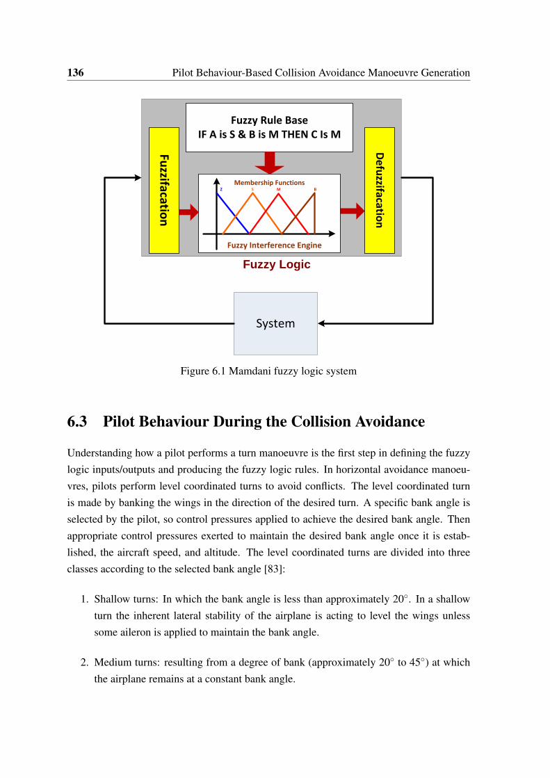
136 Pilot Behaviour-Based Collision Avoidance Manoeuvre Generation
Fuzzy Rule BaseIF A is S & B is M THEN C Is M
De
fuzzifacatio
n
Fuzzy Interference Engine
Membership Functions
Fuzzifacatio
n
Z S M B
Fuzzy Logic
System
Figure 6.1 Mamdani fuzzy logic system
6.3 Pilot Behaviour During the Collision Avoidance
Understanding how a pilot performs a turn manoeuvre is the first step in defining the fuzzylogic inputs/outputs and producing the fuzzy logic rules. In horizontal avoidance manoeu-vres, pilots perform level coordinated turns to avoid conflicts. The level coordinated turnis made by banking the wings in the direction of the desired turn. A specific bank angle isselected by the pilot, so control pressures applied to achieve the desired bank angle. Thenappropriate control pressures exerted to maintain the desired bank angle once it is estab-lished, the aircraft speed, and altitude. The level coordinated turns are divided into threeclasses according to the selected bank angle [83]:
1. Shallow turns: In which the bank angle is less than approximately 20◦. In a shallowturn the inherent lateral stability of the airplane is acting to level the wings unlesssome aileron is applied to maintain the bank angle.
2. Medium turns: resulting from a degree of bank (approximately 20◦ to 45◦) at whichthe airplane remains at a constant bank angle.
6.3 Pilot Behaviour During the Collision Avoidance 137
3. Steep turns: The turns that result from a degree of bank (45◦ or more).
The Airplane Flying Handbook [83] (published by FAA) gives more details about thelevel turns characteristics.
6.3.1 Performing the Coordinated Level Turns
Steep turns are generally flown at 45◦ bank angles, in both directions, and to a specificheading, and the altitude must be maintained within 100 feet. The following steps give ageneral summary of the procedure that is used by the pilot to achieve a level steep turn [83]:
1. Roll into the turn: The bank angle is changed from zero towards 45◦.
2. When the bank angle passes through 30◦ of bank, the back elevator pressure shouldbe smoothly increased to maintain the altitude.
3. As the turn continues, increased elevator back pressure will be needed in order tomaintain the altitude. Additional back-elevator pressure increases the angle of at-tack, which results in an increase in drag. Consequently, power must be increased tomaintain the entry altitude and airspeed.
4. The roll out from the turn should be timed so that the wings reach level flight whenthe airplane is exactly on the predetermined heading. While the recovery is beingmade, back-elevator pressure is gradually released and power reduced, as necessary,to maintain the altitude and airspeed. When beginning to roll out of the turn to thepredetermined heading, lead the roll out by one-half the number of degrees of thebank angle. For example, in a 30◦ bank turn, begin to level the wings 15◦ degreesbefore reaching the desired heading.
5. Lower the nose, as the back pressure required to maintain level flight during the turnwill cause the airplane to climb once the turn has been completed.
It can be noticed that at a specific speed and altitude values, there are three parameters thatcontrol the turn: the bank angle, the roll rate, and the heading angle. 1. The next sectionsshow how the bank angle and the roll rate are calculated based on the pilot experience,and used in collision avoidance manoeuvre generation process. Hence, the UAV avoidancemanoeuvre can mimic a manned aircraft during the conflict.
1In this thesis the selected heading angles for the conflict scenarios are discussed in Chapter 5

138 Pilot Behaviour-Based Collision Avoidance Manoeuvre Generation
6.3.2 Avoidance Manoeuvre Bank Angle Selection
In the collision avoidance manoeuvres pilots usually avoid the collision by using medium,or steep coordinated level turns. For example, one of the bank angles 30◦, 45◦, or 60◦ isselected to perform the turn part of the collision avoidance manoeuvre. The selected bankangle depends on the conflict scenario:
• 30◦ bank angle is used for conflict scenarios where:
– The speed of the aircraft V is very low, near the minimum speed, so a higherbank angle at the low speed may cause stall (see Section 5.2.1), and
– the time to collision is very large (Tc > 35s).
• Banking by 60◦, or the maximum bank angle, which is limited by the maximumnormal load factor as given by (5.9), is used in critical conflict scenarios where:
– The speed of the aircraft V is very high, and
– the time to collision is very short (Tc < 12s).
• Generally speaking a bank angle of 45◦ is the pilot’s preferred bank angle in most ofconflict scenarios.
The pilot selects a specific value of the bank angle and often uses that value for most ofconflict scenarios. It is easier for the pilot if they can achieve the coordinated level turn ata bank angle they are familiar with rather than banking at different angles. However, thisdiffers from pilot to pilot based on their training and experience. In this chapter a bank angleof 45◦ is considered for all scenarios.
6.3.3 Avoidance Manoeuvre Roll Rate Calculation
To achieve the roll angle, range of a roll rates may be applied. For example, the pilot willtry to change the bank angle from zero to 45◦ rapidly (big roll rate) if the time to collisionis within the short range (Tc < 20s) and the aircraft speed is in medium/high ranges. Bankangle is changed slowly (small roll rate) if the time to collision belongs to a large range(Tc > 20s) and the aircraft speed belongs to slow/medium ranges. The fuzzy logic techniqueis used to represent the pilot behaviour in generating the roll rate for the turn part of theavoidance manoeuvre. The fuzzy inputs are the time to collision Tc, and the UAV speed

6.3 Pilot Behaviour During the Collision Avoidance 139
V . The output is the roll rate which is sent to the avoidance manoeuvre generation processto generate the avoidance manoeuvre trajectory profiles. Figures 6.2, and 6.3 show themembership functions of the time to collision Tc and the UAV speed V respectively. Thetime and the speed ranges are selected based on pilot experience (which may differ fromone pilot to another):
• S denotes time to collision membership function Small.
• M denotes time to collision membership function Medium.
• B denotes time to collision membership function Big.
The same notations are used to represent the UAV speed membership functions.
Time (sec)
µ(TC)
S M B
15 20 30
Figure 6.2 Time to collide membership functions
SpeedVmin Vmax
µ(v)
S M B
Figure 6.3 Speed membership functions

140 Pilot Behaviour-Based Collision Avoidance Manoeuvre Generation
Figure 6.4 shows the membership functions of the roll rate (the output of the fuzzysystem), where:
• S denotes roll rate membership function Small
• M denotes roll rate membership function Medium
• B denotes roll rate membership function Big
• VB denotes roll rate membership function Very Big
µ(Φ)
S BM VB
Φmax Φ(rad/s)Φmin
Figure 6.4 Bank Angle (output) membership functions
The maximum allowable value for the roll rate depends on the minimum allowable timeto achieve a certain bank angle. The minimum allowable time to achieve a specific roll angledepends on the aircraft type and the speed. However, for small aircraft this time is as shortas one second for 90◦ degree roll [65]. Table 6.1 shows the possible rules for the decisionmaking that are established by using if-then statements based on the pilot’s experience. Therules map Tc and V to roll rate φ . For example, the first rule in the table is(IF Tc is SmallAND V is Small THEN φ is Very Big).
Table 6.1 Fuzzy inference engine (the aircraft starts manoeuvreing first)
V
Tc Small Medium Big
Small VB M S
Medium VB B M
Big VB VB B

6.4 Avoidance Manoeuvre Parameterisation 141
It is worth mentioning here that in some conflict scenarios, where both the aircraft andthe intruder are supposed to perform avoidance manoeuvres, the pilot’s reaction dependsalso on the intruder’s behaviour. For example, in head-on conflict scenarios, where boththe aircraft and the intruder should change their directions (right/left) to avoid the collision,the pilot’s reaction, when the intruder starts the avoidance manoeuvre before the pilot does,is different from the pilot reaction when he/she starts the manoeuvre before the intruder.Table 6.2 shows the possible rules for the decision making when the intruder performs theavoidance manoeuvre before the UAV, where ‘X’ denotes to hold the current states (i.e.without changing the speed, direction, and altitude). However, the behaviour of the intruderis not considered in this thesis.
Table 6.2 Fuzzy inference engine (the intruder starts manoeuvreing first)
V
Tc Small Medium Big
Small VB S X
Medium VB M X
Big VB B X
6.4 Avoidance Manoeuvre Parameterisation
The pilot’s reaction to avoid a collision is to change the aircraft direction according to therules of the air, by changing the aircraft heading to a specific heading through a level coor-dinated turn. However, as discussed in the previous section, although the heading and bankangles are predetermined the amount of roll rate that is demanded to achieve the bank angledepends on the time to collision and the UAV speed. The fuzzy logic algorithm generatesthe roll rate based on the pilot reaction to the conflict scenario. Hence, avoidance manoeu-vre trajectory profiles can be produced by using the generated roll rate, and the predefinedvalues of bank angle and heading angle. This section shows how the roll rate is used inthe avoidance manoeuvre trajectory profiles calculation. Figure 6.5 shows roll rate that isused to change the UAV bank angle from the level wing state (φo = 0) to a predeterminedbank angle φ1 at a specific roll rate φ1 during the time period Tr1. Then keep banking at theconstant bank angle φ1 for a duration of time Tr2, finally leveling the wing over the intervalTr3.
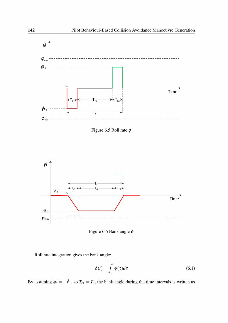
142 Pilot Behaviour-Based Collision Avoidance Manoeuvre Generation
Ø
Ømax
Ømax
Tr
Tr1 Tr2 Tr3
Time
Ø 1
Ø 3
to
Figure 6.5 Roll rate φ
Ø
Tr
Tr1 Tr2 Tr3
Time
Ø 0
Ømax
Ø 1
to
Figure 6.6 Bank angle φ
Roll rate integration gives the bank angle:
φ(t) =∫ t
0φ(τ)dτ (6.1)
By assuming φ3 = −φ1, so Tr1 = Tr3 the bank angle during the time intervals is written as

6.4 Avoidance Manoeuvre Parameterisation 143
follows:
φ(t) =
φ1t ; 0 ≤ t ≤ Tr1
φ1 ; Tr1 ≤ t ≤ Tr1 +Tr2
φ1 − φ1t ; Tr1 +Tr2 ≤ t ≤+Tr
(6.2)
where the initial time is assumed to be zero t0 = 0, and φ1 =φ1Tr1
. The bank angle is shownin Figure 6.6.
The task now is to find the values of the time intervals (Tr1, Tr2, Tr3) as functions of thegenerated roll rate φ1, the predefined heading angle ∆ψ , and the predefined bank angle φ1:
1. Time period Tr1, and Tr3 are given by:
Tr1 = Tr3 =φ1
φ1(6.3)
2. Time duration Tr2: During this period the UAV bank angle has a constant value equalto φ1. The total heading change during the total rolling time Tr must be equal to apredetermined value ∆ψ = ψ(Tr) (assuming ψ0 = 0). The relationship between theheading rate and bank angle is given:
ψ(t) =gV
tan(φ(t)) (6.4)
Figure 6.7 shows the heading rate during the total rolling time interval Tr that pro-duced by using (6.4).
Tr
Tr1 Tr2 Tr3
Timeto
.
Ψ
.
Ψ
1
Ψ.Ø .
Figure 6.7 The heading rate
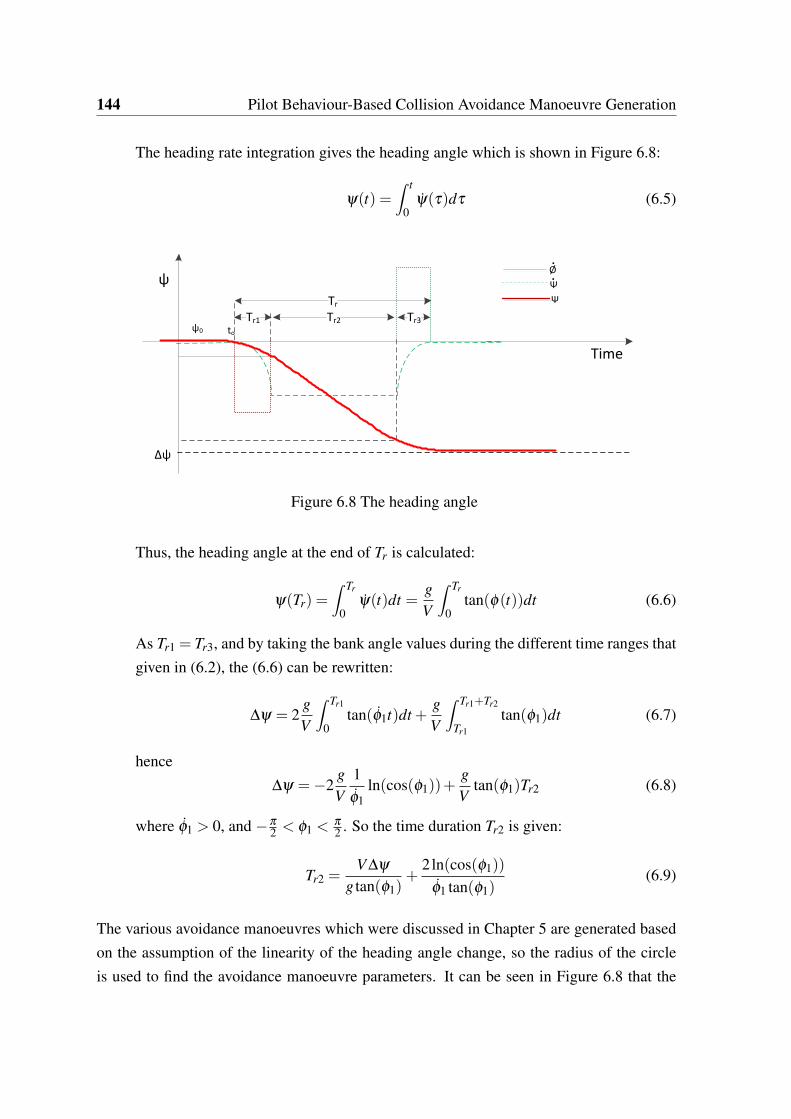
144 Pilot Behaviour-Based Collision Avoidance Manoeuvre Generation
The heading rate integration gives the heading angle which is shown in Figure 6.8:
ψ(t) =∫ t
0ψ(τ)dτ (6.5)
ψ
Tr
Tr1 Tr2 Tr3
Time
ψ0
Δψ
to
Ψ.Ø .
Ψ
Figure 6.8 The heading angle
Thus, the heading angle at the end of Tr is calculated:
ψ(Tr) =∫ Tr
0ψ(t)dt =
gV
∫ Tr
0tan(φ(t))dt (6.6)
As Tr1 = Tr3, and by taking the bank angle values during the different time ranges thatgiven in (6.2), the (6.6) can be rewritten:
∆ψ = 2gV
∫ Tr1
0tan(φ1t)dt +
gV
∫ Tr1+Tr2
Tr1
tan(φ1)dt (6.7)
hence∆ψ =−2
gV
1φ1
ln(cos(φ1))+gV
tan(φ1)Tr2 (6.8)
where φ1 > 0, and −π
2 < φ1 <π
2 . So the time duration Tr2 is given:
Tr2 =V ∆ψ
g tan(φ1)+
2ln(cos(φ1))
φ1 tan(φ1)(6.9)
The various avoidance manoeuvres which were discussed in Chapter 5 are generated basedon the assumption of the linearity of the heading angle change, so the radius of the circleis used to find the avoidance manoeuvre parameters. It can be seen in Figure 6.8 that the

6.4 Avoidance Manoeuvre Parameterisation 145
heading angle is nonlinear, hence the turn of the avoidance manoeuvre is not a circle. Thus,the parameters of the proposed manoeuvres must be modified:
1. Head-on/Overtaking avoidance manoeuvre (see Section 5.2.2):
• The time periods T1 and T3 are modified to be equal to the total rolling time Tr.
• The distance D1, which is used to calculate D2, hence the time period T2 ismodified to:
D1 = y(Tr) (6.10)
where y(Tr) is the projection of the UAV position on the y-axis at the end oftime period Tr. However, if the summation of traveled distances during timeperiods T1, and T3 is greater or equal to the minimum clearance distance dc thenthe time period T2 = 0 (i.e. if 2y(Tr)≥ dc then T2 = 0).
2. The RSL avoidance manoeuvre (see Section 5.3.1):
• The time periods T1 and T3 are modified to be equal to the total rolling time Tr.
• The projection of the distance between the UAV and the intruder on the y-axis,which is given by (5.20), is modified to:
dub2 = Ry0 − (y(Tr)+db1) (6.11)
3. The RS-LS avoidance manoeuvre (see Section 5.3.2): The time periods T1 in the RSpart, and T3 in the LS part are modified to be equal to the total rolling time Tr.
4. The circle avoidance manoeuvre (see Section 5.3.3):
• The time period Tt is modified to be equal to the total rolling time period Tr.
• The condition to perform the circle manoeuvre is given by:
Rx0 ≤ x(Tr
4)+dc(min)−
Tr
4Vc sin(θc) (6.12)
The UAV positions y(Tr), and x(Tr4 ) are calculated by using a numerical method as the ana-
lytic solution is hard to be achieved due to the nonlinearity of the heading rates and heading
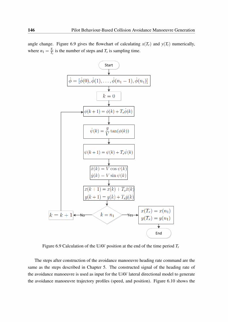
146 Pilot Behaviour-Based Collision Avoidance Manoeuvre Generation
angle change. Figure 6.9 gives the flowchart of calculating x(Tr) and y(Tt) numerically,where n1 =
TrTs
is the number of steps and Ts is sampling time.
No
Start
End
Yes
Figure 6.9 Calculation of the UAV position at the end of the time period Tr
The steps after construction of the avoidance manoeuvre heading rate command are thesame as the steps described in Chapter 5. The constructed signal of the heading rate ofthe avoidance manoeuvre is used as input for the UAV lateral directional model to generatethe avoidance manoeuvre trajectory profiles (speed, and position). Figure 6.10 shows the

6.4 Avoidance Manoeuvre Parameterisation 147
flowchart of the avoidance manoeuvre generation algorithm using fuzzy logic techniques
Start
(Right/Left) manoeuvre; Tm; Tc; Ø1; V; ΔΨT1
Generate speed and position profiles by applying the calculated heading rate on UAV lateral directional model
Method selection
Curve fit the generated speed profiles to calculate the Bezier curve coefficients
Calculate all profiles (position, speed, acceleration, and rate of acceleration)
Send the generated speed and position profiles to (LTP) algorithm
Send the trajectory profiles to the inverse dynamics algorithm which generates the command signals
End
Calculate time intervalsTr1; Tr2;Tr3;T1;T2;T3;T4
Generate by using fuzzy Logic technique Ø1Ø1
Generate the roll rate signal Ø .
Generate the heading rate signal ψ.
Figure 6.10 Avoidance manoeuvre generation algorithm flowchart
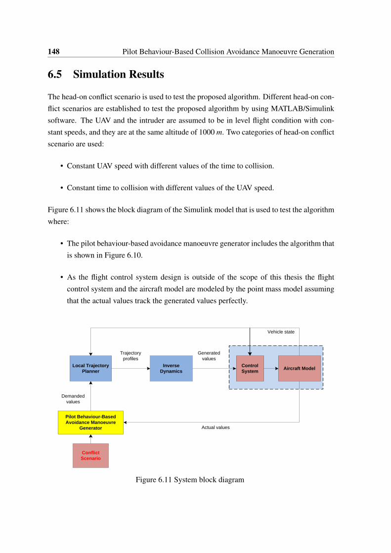
148 Pilot Behaviour-Based Collision Avoidance Manoeuvre Generation
6.5 Simulation Results
The head-on conflict scenario is used to test the proposed algorithm. Different head-on con-flict scenarios are established to test the proposed algorithm by using MATLAB/Simulinksoftware. The UAV and the intruder are assumed to be in level flight condition with con-stant speeds, and they are at the same altitude of 1000 m. Two categories of head-on conflictscenario are used:
• Constant UAV speed with different values of the time to collision.
• Constant time to collision with different values of the UAV speed.
Figure 6.11 shows the block diagram of the Simulink model that is used to test the algorithmwhere:
• The pilot behaviour-based avoidance manoeuvre generator includes the algorithm thatis shown in Figure 6.10.
• As the flight control system design is outside of the scope of this thesis the flightcontrol system and the aircraft model are modeled by the point mass model assumingthat the actual values track the generated values perfectly.
Inverse
DynamicsAircraft Model
Local Trajectory
Planner
Trajectory
profiles
Vehicle state
Conflict
Scenario
Pilot Behaviour-Based
Avoidance Manoeuvre
Generator
Control
System
Actual values
Demanded
values
Generated
values
Figure 6.11 System block diagram

6.5 Simulation Results 149
6.5.1 Constant V with Different Values of Tc
These scenarios are designed to show the effect of the time to collision Tc on the avoidancemanoeuvre while the UAV speed V is constant for all scenarios. Figure 6.12 shows threehead-on conflict scenarios where the UAV speed V and the intruder speed Vi are constantin all scenarios, but the intruder initial position is different for each scenario so the time tocollision is different for each scenario.
ΔΨT1 =60o
dc>500 m
V=50 m/s Vi=50 m/s
Range1=3200m
Tc=32sUAV
Range2=2000m
Range3=1400m
Vi=50 m/s Vi=50 m/s
Scenario1Scenario2Scenario3Tc=20sTc=14s
Figure 6.12 Head-on conflict scenarios (1,2, and 3)
Table 6.3 shows the avoidance manoeuvre parameters for each scenario. It can be seenthat the heading rate is increased as the time to collision decreased. Hence, the turning partof the avoidance manoeuvre is performed faster.
Table 6.3 Conflict scenarios (1,2, and 3): V =Vi = 50m.s−1, ∆ψ = 60o, φ = 45o
Parameter Scenario1 Scenario2 Scenario3
Range [m] 3200 2000 1400
Tc [s] 32 20 14
φ [deg/s] 14.89 35 95
Tr1 [s] 3.02 1.29 0.47
Tr2 [s] 2.67 4.2 4.92
T1 [s] 8.71 6.77 5.87
T2 [s] 2.27 4.28 5.18
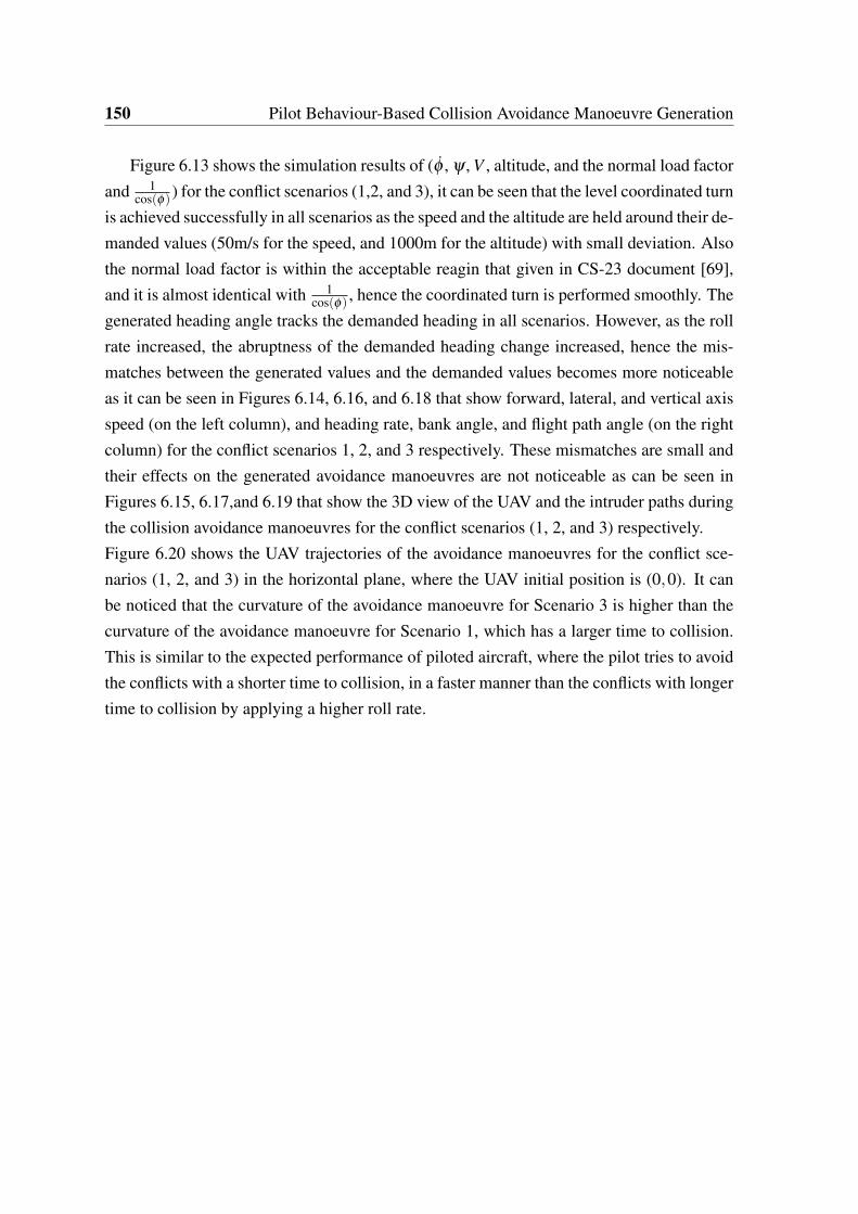
150 Pilot Behaviour-Based Collision Avoidance Manoeuvre Generation
Figure 6.13 shows the simulation results of (φ , ψ , V , altitude, and the normal load factorand 1
cos(φ)) for the conflict scenarios (1,2, and 3), it can be seen that the level coordinated turnis achieved successfully in all scenarios as the speed and the altitude are held around their de-manded values (50m/s for the speed, and 1000m for the altitude) with small deviation. Alsothe normal load factor is within the acceptable reagin that given in CS-23 document [69],and it is almost identical with 1
cos(φ) , hence the coordinated turn is performed smoothly. Thegenerated heading angle tracks the demanded heading in all scenarios. However, as the rollrate increased, the abruptness of the demanded heading change increased, hence the mis-matches between the generated values and the demanded values becomes more noticeableas it can be seen in Figures 6.14, 6.16, and 6.18 that show forward, lateral, and vertical axisspeed (on the left column), and heading rate, bank angle, and flight path angle (on the rightcolumn) for the conflict scenarios 1, 2, and 3 respectively. These mismatches are small andtheir effects on the generated avoidance manoeuvres are not noticeable as can be seen inFigures 6.15, 6.17,and 6.19 that show the 3D view of the UAV and the intruder paths duringthe collision avoidance manoeuvres for the conflict scenarios (1, 2, and 3) respectively.Figure 6.20 shows the UAV trajectories of the avoidance manoeuvres for the conflict sce-narios (1, 2, and 3) in the horizontal plane, where the UAV initial position is (0,0). It canbe noticed that the curvature of the avoidance manoeuvre for Scenario 3 is higher than thecurvature of the avoidance manoeuvre for Scenario 1, which has a larger time to collision.This is similar to the expected performance of piloted aircraft, where the pilot tries to avoidthe conflicts with a shorter time to collision, in a faster manner than the conflicts with longertime to collision by applying a higher roll rate.

6.5 Simulation Results 151
0 5 10 15 20-100
0
100
d
/dt
[deg/s
]
Scenario1: Tc=32s, V=50m/s
0 5 10 15 20
-50
0
50
[
deg]
d
g
0 5 10 15 20
40
50
60
V [
m/s
]
Vd
Vg
0 5 10 15 20995
1000
1005
Altitude [
m]
Time [s]
0 5 10 15 200
1
2
Load factor
1/cos()
0 5 10 15 20-100
0
100
Scenario2: Tc=20s, V=50m/s
0 5 10 15 20
-50
0
50
0 5 10 15 20
40
50
60
0 5 10 15 20995
1000
1005
Time [s]
0 5 10 15 200
1
2
0 5 10 15 20-100
0
100
Scenario3: Tc=14s, V=50m/s
0 5 10 15 20
-50
0
50
0 5 10 15 20
40
50
60
0 5 10 15 20995
1000
1005
Time [s]
0 5 10 15 200
1
2
Figure 6.13 The simulation results of (φ , ψ , V , and altitude) for scenarios (1, 2, and 3)

152 Pilot Behaviour-Based Collision Avoidance Manoeuvre Generation
0 10 20 30
-10
0
10
d
/dt
[deg.s
-1]
0 10 20 30
-50
0
50
[
deg]
0 10 20 30-5
0
5
[deg]
Time [s]
0 10 20 30
20
30
40
50
60
Forw
ard
speed [
m.s
-1]
0 10 20 30
-40
-20
0
Late
ral speed [
m.s
-1]
0 10 20 30
-2
0
2
Time [sec]
Vert
ical speed [
m.s
-1]
dd/dt
dg/dt
d
g
d
g
ud
ug
vd
vg
wd
wg
Figure 6.14 Scenario1 simulation results (Left): u, v, and w; (Right): ψ , φ , and γ
0
1000
2000
3000
4000
-1000-800
-600-400
-2000
200400
600
800
900
1000
1100
1200
X [m]
X: 1373
Y: -502.7
Z: 1001
X: 3200
Y: 0
Z: 1000
Y [m]
X: 0
Y: 0
Z: 1000
X: 1600
Y: -1.959e-013
Z: 1000
Z [
m]
Demanded trajectory
Generated trajectory
Intruder trajectory
UAV initial position
Intruder initial position
UAV psosition at t=Tc
CP (Intruder position at t=Tc)
Figure 6.15 Scenario 1: 3D view of the UAV, and the intruder trajectories

6.5 Simulation Results 153
0 10 20 30
-10
0
10
d
/dt
[deg.s
-1]
dd/dt
dg/dt
0 10 20 30
-50
0
50
[
deg]
d
g
0 10 20 30-5
0
5
[d
eg]
Time [s]
d
g
0 10 20 30
20
30
40
50
60
Forw
ard
speed [
m.s
-1]
ud
ug
0 10 20 30
-40
-20
0
Late
ral speed [
m.s
-1]
vd
vg
0 10 20 30
-2
0
2
Time [sec]
Vert
ical speed [
m.s
-1]
wd
wg
Figure 6.16 Scenario2 simulation results (Left): u, v, and w; (Right): ψ , φ , and γ
-500
0
500
1000
1500
2000
-800
-600
-400
-200
0
200
800
900
1000
1100
1200
X [m]
X: 753.7
Y: -503
Z: 1000
X: 2000
Y: 0
Z: 1000
Y [m]
X: 0
Y: 0
Z: 1000
X: 1000
Y: -1.225e-13
Z: 1000
Z [
m]
Demanded trajectory
Generated trajectory
Intruder trajectory
UAV initial position
Intruder initial position
UAV psosition at t=Tc
CP (Intruder position at t=Tc)
Figure 6.17 Scenario 2: 3D view of the UAV, and the intruder trajectories
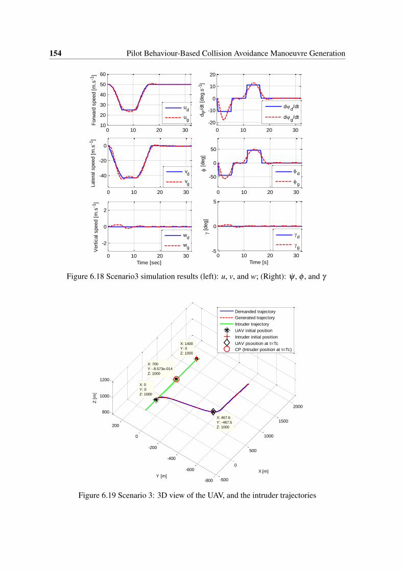
154 Pilot Behaviour-Based Collision Avoidance Manoeuvre Generation
0 10 20 30
-20
-10
0
10
20
d
/dt
[deg.s
-1]
dd/dt
dg/dt
0 10 20 30
-50
0
50
[
deg]
d
g
0 10 20 30-5
0
5
[deg]
Time [s]
d
g
0 10 20 3010
20
30
40
50
60
Forw
ard
speed [
m.s
-1]
ud
ug
0 10 20 30
-40
-20
0
Late
ral speed [
m.s
-1]
vd
vg
0 10 20 30
-2
0
2
Time [sec]
Vert
ical speed [
m.s
-1]
wd
wg
Figure 6.18 Scenario3 simulation results (left): u, v, and w; (Right): ψ , φ , and γ
-500
0
500
1000
1500
2000
-800
-600
-400
-200
0
200
800
1000
1200
X [m]
X: 467.6
Y: -467.5
Z: 1000
X: 1400
Y: 0
Z: 1000
Y [m]
X: 700
Y: -8.573e-014
Z: 1000
X: 0
Y: 0
Z: 1000
Z [
m]
Demanded trajectory
Generated trajectory
Intruder trajectory
UAV initial position
Intruder initial position
UAV psosition at t=Tc
CP (Intruder position at t=Tc)
Figure 6.19 Scenario 3: 3D view of the UAV, and the intruder trajectories
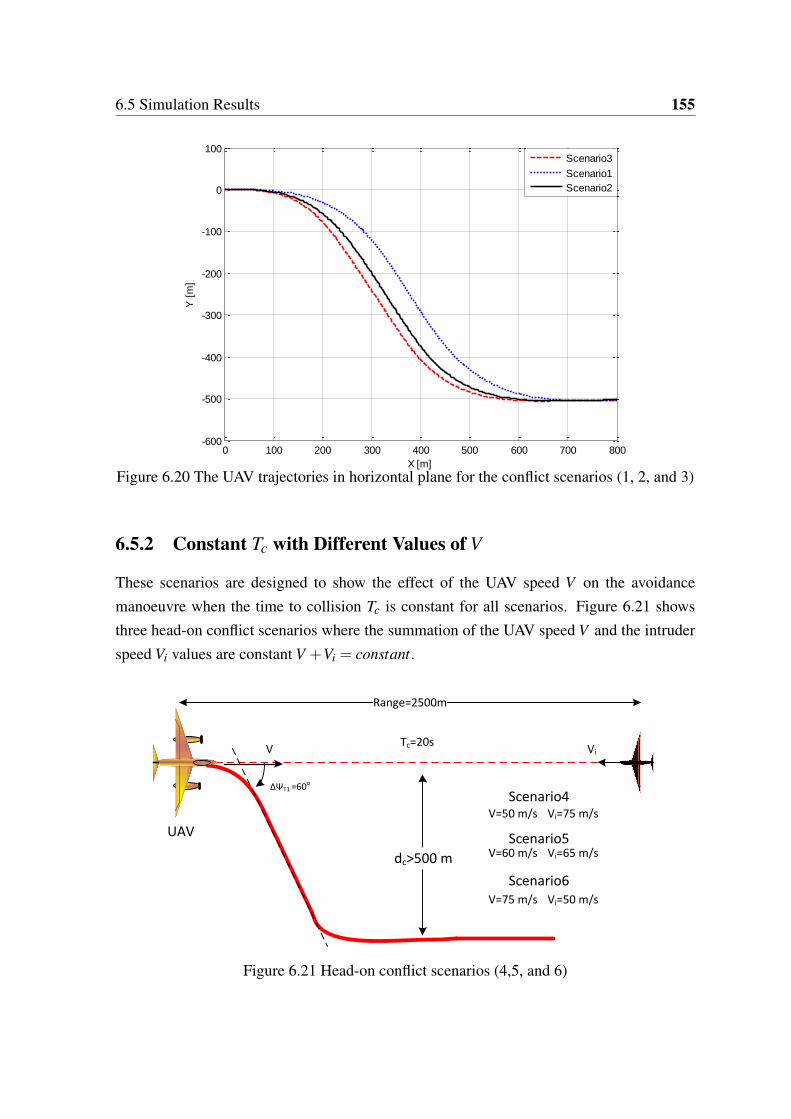
6.5 Simulation Results 155
0 100 200 300 400 500 600 700 800-600
-500
-400
-300
-200
-100
0
100
Y [
m]
X [m]
Scenario3
Scenario1
Scenario2
Figure 6.20 The UAV trajectories in horizontal plane for the conflict scenarios (1, 2, and 3)
6.5.2 Constant Tc with Different Values of V
These scenarios are designed to show the effect of the UAV speed V on the avoidancemanoeuvre when the time to collision Tc is constant for all scenarios. Figure 6.21 showsthree head-on conflict scenarios where the summation of the UAV speed V and the intruderspeed Vi values are constant V +Vi = constant.
ΔΨT1 =60o
dc>500 m V=60 m/s
Range=2500m
UAVVi=75 m/s
Scenario4
Scenario5
Scenario6
Tc=20s
V=50 m/s
Vi=65 m/s
V=75 m/s Vi=50 m/s
V Vi
Figure 6.21 Head-on conflict scenarios (4,5, and 6)
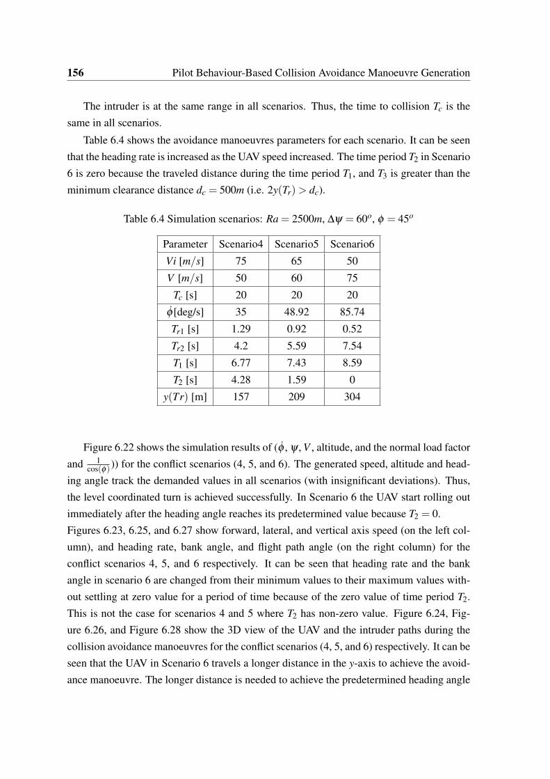
156 Pilot Behaviour-Based Collision Avoidance Manoeuvre Generation
The intruder is at the same range in all scenarios. Thus, the time to collision Tc is thesame in all scenarios.
Table 6.4 shows the avoidance manoeuvres parameters for each scenario. It can be seenthat the heading rate is increased as the UAV speed increased. The time period T2 in Scenario6 is zero because the traveled distance during the time period T1, and T3 is greater than theminimum clearance distance dc = 500m (i.e. 2y(Tr)> dc).
Table 6.4 Simulation scenarios: Ra = 2500m, ∆ψ = 60o, φ = 45o
Parameter Scenario4 Scenario5 Scenario6
Vi [m/s] 75 65 50
V [m/s] 50 60 75
Tc [s] 20 20 20
φ [deg/s] 35 48.92 85.74
Tr1 [s] 1.29 0.92 0.52
Tr2 [s] 4.2 5.59 7.54
T1 [s] 6.77 7.43 8.59
T2 [s] 4.28 1.59 0
y(Tr) [m] 157 209 304
Figure 6.22 shows the simulation results of (φ , ψ , V , altitude, and the normal load factorand 1
cos(φ))) for the conflict scenarios (4, 5, and 6). The generated speed, altitude and head-ing angle track the demanded values in all scenarios (with insignificant deviations). Thus,the level coordinated turn is achieved successfully. In Scenario 6 the UAV start rolling outimmediately after the heading angle reaches its predetermined value because T2 = 0.Figures 6.23, 6.25, and 6.27 show forward, lateral, and vertical axis speed (on the left col-umn), and heading rate, bank angle, and flight path angle (on the right column) for theconflict scenarios 4, 5, and 6 respectively. It can be seen that heading rate and the bankangle in scenario 6 are changed from their minimum values to their maximum values with-out settling at zero value for a period of time because of the zero value of time period T2.This is not the case for scenarios 4 and 5 where T2 has non-zero value. Figure 6.24, Fig-ure 6.26, and Figure 6.28 show the 3D view of the UAV and the intruder paths during thecollision avoidance manoeuvres for the conflict scenarios (4, 5, and 6) respectively. It can beseen that the UAV in Scenario 6 travels a longer distance in the y-axis to achieve the avoid-ance manoeuvre. The longer distance is needed to achieve the predetermined heading angle

6.5 Simulation Results 157
(ψ = 60◦), because the higher speed turn has a larger radius of turn. Figure 6.29 shows theposition profiles of the avoidance manoeuvres for the conflict scenarios (4, 5, and 6) in thehorizontal plane, where the UAV initial position is (0,0).
0 5 10 15 20-100
0
100
d
/dt
[deg/s
]
Scenario4: Tc=20s, V=50m/s
0 10 20
-50
0
50
[
deg]
d
g
0 10 20
40
60
80
V [
m/s
]
Vd
Vg
0 10 20995
1000
1005
Altitude [
m]
0 10 200
1
2
3
Time [s]
Load factor
1/cos()
0 10 20-100
0
100
Scenario5: Tc=20s, V=60m/s
0 10 20
-50
0
50
0 10 20
40
60
80
0 10 20995
1000
1005
0 10 200
1
2
3
Time [s]
0 10 20-100
0
100
Scenario6: Tc=20s, V=75m/s
0 10 20
-50
0
50
0 10 20
40
60
80
0 10 20995
1000
1005
0 10 200
1
2
3
Time [s]
Figure 6.22 The simulation results of (φ , ψ , V , and altitude) for scenarios (4, 5, and 6)

158 Pilot Behaviour-Based Collision Avoidance Manoeuvre Generation
0 10 20 30
-10
0
10
d
/dt
[deg.s
-1]
dd/dt
dg/dt
0 10 20 30
-50
0
50
[
deg]
d
g
0 10 20 30-5
0
5
[d
eg]
Time [s]
d
g
0 10 20 30
20
30
40
50
60
Forw
ard
speed [
m.s
-1]
ud
ug
0 10 20 30
-40
-20
0
Late
ral speed [
m.s
-1]
vd
vg
0 10 20 30
-2
0
2
Time [sec]
Vert
ical speed [
m.s
-1]
wd
wg
Figure 6.23 Scenario4 simulation results (left): u, v, and w; (Right): ψ , φ , and γ
-500
0
500
1000
1500
2000
2500
-800
-600
-400
-200
0
200
800
900
1000
1100
1200
X [m]
X: 764.7
Y: -502.8
Z: 1000
Y [m]
X: 2500
Y: 0
Z: 1000
X: 0
Y: 0
Z: 1000
X: 1000
Y: -1.837e-013
Z: 1000
Z [
m]
Demanded trajectory
Generated trajectory
Intruder trajectory
UAV initial position
Intruder initial position
UAV psosition at t=Tc
CP (Intruder position at t=Tc)
Figure 6.24 Scenario 4: 3D view of the UAV, and the intruder trajectories

6.5 Simulation Results 159
0 10 20 30
-10
0
10
d
/dt
[deg.s
-1]
dd/dt
dg/dt
0 10 20 30
-50
0
50
[
deg]
d
g
0 10 20 30-5
0
5
[d
eg]
Time [s]
d
g
0 10 20 30
20
40
60
Forw
ard
speed [
m.s
-1]
ud
ug
0 10 20 30
-60
-40
-20
0
Late
ral speed [
m.s
-1]
vd
vg
0 10 20 30
-2
0
2
Time [sec]
Vert
ical speed [
m.s
-1]
wd
wg
Figure 6.25 Scenario5 simulation results (left): u, v, and w; (Right): ψ , φ , and γ
-500
0
500
1000
1500
2000
2500
-800-600
-400-200
0200
800
900
1000
1100
1200
X [m]
X: 987
Y: -503.1
Z: 1000
Y [m]
X: 2500
Y: 0
Z: 1000
X: 0
Y: 0
Z: 1000
X: 1200
Y: -1.592e-013
Z: 1000
Z [
m]
Demanded trajectory
Generated trajectory
Intruder trajectory
UAV initial position
Intruder initial position
UAV position at t=Tc
CP (Intruder position at t=Tc)
Figure 6.26 Scenario 5: 3D view of the UAV, and the intruder trajectories

160 Pilot Behaviour-Based Collision Avoidance Manoeuvre Generation
0 10 20 30
-10
0
10
d
/dt
[deg.s
-1]
dd/dt
dg/dt
0 10 20 30
-50
0
50
[
deg]
d
g
0 10 20 30-5
0
5
[deg]
Time [s]
d
g
0 10 20 30
40
60
80
Forw
ard
speed [
m.s
-1]
ud
ug
0 10 20 30
-80
-60
-40
-20
0
Late
ral speed [
m.s
-1]
vd
vg
0 10 20 30
-2
0
2
Time [sec]
Vert
ical speed [
m.s
-1]
wd
wg
Figure 6.27 Scenario6 simulation results (left): u, v, and w; (Right): ψ , φ , and γ
-500
0
500
1000
1500
2000
2500
-800-600
-400-200
0200
800
900
1000
1100
1200
X [m]
X: 1269
Y: -609.6
Z: 1000
Y [m]
X: 2500
Y: 0
Z: 1000
X: 1500
Y: -1.225e-013
Z: 1000
X: 0
Y: 0
Z: 1000
Z [
m]
Demanded trajectory
Generated trajectory
Intruder trajectory
UAV initial position
Intruder initial position
UAV position at t=Tc
CP (Intruder position at t=Tc)
Figure 6.28 Scenario 6: 3D view of the UAV, and the intruder trajectories

6.6 Summary 161
0 200 400 600 800 1000 1200-700
-600
-500
-400
-300
-200
-100
0
100
Y [
m]
X [m]
Scenario4 (V=50m/s)
Scenario5 (V=60m/s)
Scenario6 (V=75m/s)
Figure 6.29 The UAV trajectories in the horizontal plane for the conflict scenarios (4, 5, and6)
6.6 Summary
This chapter discusses how pilot experience can be used in the collision avoidance ma-noeuvre generation process for the UAV. This chapter presents a proposal for linking theavoidance manoeuvre’s parameters with the conflict scenario’s parameters using the pilotbehaviour during the conflict. This is to augment the pilot experiences in the avoidancemanoeuvre generation process. In manned aircraft, pilots use their experience to initiate thesuitable manoeuvre to avoid the conflict. The fuzzy logic technique is proposed to modelthe pilot actions in generating the avoidance manoeuvre for different conflict scenarios.

Chapter 7
Conclusions and Recommendations forFuture Work
Operation of UAV’s in civil airspace is restricted by the policies of aviation authorities whichrequire full compliance with rules and obligations that apply for manned aircraft. Trajectorytracking and collision avoidance are issues that a UAV must deal with in a way that givesthe UAV the ability to avoid conflict situations. Thus, any UAV that will be operated incivil/non-segregated airspace must be equipped with a collision avoidance system that hasthe ability to avoid conflict scenarios in full compliance with the rules of the air. The mainaim of this thesis is to develop a control algorithm for collision avoidance system for aircraftthat are flying under VFR conditions. The developed algorithm could be used at differentlevels of the aircraft autonomy. For example, the developed algorithm can be used as an ad-visory system for manned aircraft to help the pilot for see and avoid, or it can be a guidancesystem for a UAV in order to enable it to fly in civil airspace. The following sections giveconclusions for the proposed algorithms and techniques that have been developed in thisthesis and discusses their limitations, as well as giving some recommendations for futurework.
7.1 Local Trajectory Planning Algorithm
An optimal local trajectory generation that uses B-splines is proposed for a real-time col-lision avoidance algorithm. Online avoidance manoeuvre generation, optimisation, andglobal trajectory tracking for different conflict scenarios are tested successfully in a sim-ulation environment. The predicted trajectory is generated by using MPC techniques. Es-sentially, a finite-horizon optimal control problem is periodically solved in real-time hence
164 Conclusions and Recommendations for Future Work
updating the aircraft trajectory to avoid obstacles and track a predefined global trajectory.The aircraft and obstacle constraints are augmented in the cost function using a penaltyfunction method. The computational time for the real-time collision avoidance algorithm isreduced significantly by using output space to formulate the optimal control problem, andaugmenting the vehicle/obstacle constraints in the cost function. A coarse grid approachis proposed to help the optimal control problem solver to escape the local minima and en-sure sufficient coverage of the overall design space. Differential flatness of the system fora fixed wing aircraft is used to produce an inverse dynamic model for the UAV. Hence, thegenerated local trajectory profiles passed to the inverse dynamic model to generate the core-sponding control signals. The simulation results show that the proposed approach allowsthe UAV to track a predefined global trajectory, as well as avoiding collisions with differenttypes of conflict scenarios in real-time. In the simulation and for the tested scenarios theproposed algorithm successfully allows the UAV to achieve the following tasks:
1. Satisfy the UAV constraints.
2. Track a predefined global trajectory.
3. Avoid static obstacles.
4. Avoid moving obstacles.
However, the developed algorithm suffers from limitations. Some of these limitations canbe summarized:
• The intruder trajectory has been estimated using a straight projection method in whichthe intruder states are projected into the future along a single trajectory. Although thismethod is simple, there is no direct consideration of the uncertainties.
• The proposed method for avoiding local minima reduces the possibility of gettingtrapped in local minima but does not overcome it totally.
• The UAV has been modelled by a three Degree of Freedom (3-DoF) point-mass modelbased on some assumptions (e.g. still wind, zero sideslip, flight path angle γ equalspitch angle θ ).
• No effort has been directed towards investigating the effect of length of the horizontime (th), and the sampling resolution of the global trajectory on the algorithm effi-ciency.
7.2 Decision Making System 165
Some recommendations for future work are:
• A method for intruder future trajectory estimation should be developed taking intoconsideration the intruder manoeuvrability. One proposal is to develop a model thatpredicts the intruder manoeuvre based on limitations of the intruder, and uncertaintiesof measured data.
• Monte Carlo simulation should be performed for a more through evaluation of theproposed proposed algorithm.
• Test the algorithm with external disturbances (i.e. wind), and internal failures (e.g.UAV actuator failures)
• Test the algorithm with a six Degrees of Freedom (6-DoF) model of a UAV.
• As the inverse dynamics generates the command inputs for the receding horizon time,a MPC can be proposed to design the UAV controllers (in the control layer).
• The algorithm should be experimentally tested using a flight simulator, and flight test.
• Develop a more effective algorithm for the optimal control problem solver to avoidlocal minima.
7.2 Decision Making System
A multi-layer DMS is developed for a sense and avoid system based on the rules of the airin VFR conditions. The proposed DMS architecture is engineered to be implemented fordifferent functionalities for manned aircraft, and at different level of autonomy of UAS, orat different classes of the flight control modes that are specified by CAA (see Section 4.7for more details about flight control modes). For example, in manned aircraft (Class-0flight control mode) the proposed DMS can be used to reduce the overall pilot workload byperforming the flowing tasks:
1. Collisions detection and risk prioritizing (Layer-1), so the pilot will know where thetraffics are (Section 4.8.1, and Section 4.8.2).
2. Determine the collision scenario type (i.e. head-on, left/right approaching, and over-taking/overtaken) by using Layer-1, and Layer-2. This will help the pilot to decidewhat actions are needed to avoid the conflict (Section 4.8.4).

166 Conclusions and Recommendations for Future Work
3. Evaluate the collision type, and generates conflict resolution advisories (Layer-3) tohelp the pilot to initiate a safe avoidance manoeuvre (Section 4.8.5).
Currently available commercial collision avoidance systems that are used for see and avoid(e.g. the Potable Collision Avoidance System PCAS) can just perform the first task (seeSection 4.8.1). Earlier discussion shows that most of the required time for a pilot to recog-nize an approaching aircraft and initiate an avoidance manoeuvre is spent on the decisionmaking process. Hence, a decision making system that could be used as an advisory systemwill effectively save time and help the pilot to avoid the conflicts safely.For a remotely piloted UAV (Class-1 flight control mode) the proposed DMS architecturecould enhance the remote pilot awareness of the conflict, as it is can perform a decisionmaking process similar to a pilot in manned aircraft. So the remote pilot could act in thesame manner as the pilot on board in case of manned aircraft. Moreover, the remote pilotcan switch to the autonomous mode by engaging Layer-4 of the DMS which initiate a safeavoidance manoeuvre (Section 4.8.6). A GUI for the DMS is proposed for test and simula-tion purposes with a brief comparison with currently used commercial PCAS.
Some limitations of the developed DMS are:
• The type of intruder has not been considered in the decision making process. Therules of the air suggest different actions for different intruders. For example, whentwo aircraft are converging at approximately the same level, the aircraft that has theother on its right shall give way, except as follows [16]:
1. Power-driven heavier-than-air aircraft shall give way to airships, gliders andballoons
2. Airships shall give way to gliders and balloons
3. Gliders shall give way to balloons
4. Power-driven aircraft shall give way to aircraft which are seen to be towingother aircraft or objects
• The case when the intruder performs aggressive/unpridectable manoeuvres (e.g. turnleft where it supposed to turn right according to the rules of the air) are not consideredin the decision making process.

7.3 Collision Avoidance Manoeuvre Generation 167
However, the proposed DMS architecture gives flexibility for any further development layerby layer, or the whole system for research or certification purposes. Some recommendationsfor future work are:
• Develop an intruder recognition system to be added to the DMS, so the decision mak-ing process can take into consideration the type of the intruder.
• Decisions in response to aggressive/unpridectable manoeuvres by the intruder shouldbe developed.
• The system can be developed to include a cooperative operating mode. In case theUAV and the intruder are equipped with DMS, the system should work in a coordi-nated manner. For example, when an RA, or avoidance manoeuvre is initiated for con-flicting aircraft, the other aircraft will be initiated with a coordinated RA/avoidancemanoeuvre. Hence, the overall system safety is enhanced.
7.3 Collision Avoidance Manoeuvre Generation
Collision avoidance manoeuvres are proposed for a subset of the possible conflict scenarios.The proposed manoeuvres are generated to be similar to the manoeuvres that are performedby manned aircraft. A level coordinated turn is proposed for the turning part of the avoidancemanoeuvres (Section 5.2.1). This type of turn is selected according to pilot suggestions asit is the preferred manoeuvre by pilots to perform a horizontal avoidance manoeuvre insee and avoid conditions. The avoidance manoeuvres generation process takes the rulesof the air and the safety requirements into consideration. A geometric approach is used toparameterize the proposed avoidance manoeuvre. Then the parameterized manoeuvres arediscretised and used as a global trajectory to be tracked using the developed local trajectoryplanning algorithm. The collision avoidance manoeuvres are proposed for conflict scenarioswhere the UAV and the intruder are in a cruising state (constant speed level flight). Thefollowing conflict scenarios have been considered:
1. Head-on/Overtaking conflict scenarios: One type of the avoidance manoeuvre is usedfor all head-on conflict scenarios (Section 5.2.2).
2. Right approached conflict scenarios: Different cases are discussed, then, three maintypes of the avoidance manoeuvres for these cases are proposed (Section 5.2.3).
168 Conclusions and Recommendations for Future Work
The weakness with this method is ensuring that a manoeuvre has been defined for everypossible situation. Another drawback is that a limited set of scenarios has been defined,which is a subset of all possible scenarios. Hence, the effectiveness of this method cannotbe proven by just simulation and testing it for these limited number of conflict scenarios. Tostart ensuring every scenario is covered one would have to define the set of all scenarios andmake sure the set was covered. Proving that the methods work for every scenario is hardto be achieved. However, Monte Carlo simulation can be established in order to show themethod’s effectiveness. Other recommendations for future work are:
• Propose and generate avoidance manoeuvres for conflict scenarios that need a changein aircraft vertical trends (i.e. increase/decrease the decent/climb rate, or level off).Constant climb/decent rate avoidance manoeuvres can be used to avoid these type ofconflict scenarios.
• Optimal control problem can be formulated in order to optimise the generated avoid-ance manoeuvres. This can be achieved by calculating the optimal heading angle andbank angle that minimise a defined cost function. The cost function could be the dis-tance of the avoidance manoeuvre, the time of the avoidance manoeuvre, or the fuelconsumption. The resulting avoidance manoeuvre may no longer resemble a pilotgenerated avoidance manoeuvre.
7.4 Pilot Behaviour-Based Collision Avoidance ManoeuvreGeneration
A further development in avoidance manoeuvre generation algorithm is proposed by aug-menting pilot experience in the avoidance manoeuvre generation process. Hence, the UAVmimics manned aircraft behaviour in avoiding the conflict scenarios. A fuzzy logic tech-nique is proposed to represent the pilot model during the avoidance manoeuvre based on thepilot behaviour during different conflict scenarios (Section 6.3). This includes:
1. Define the fuzzy logic system inputs/outputs: The fuzzy logic system inputs/outputsare defined by determining the main factors the affect the pilot reaction and use themas inputs for the fuzzy system. This research shows that the demanded roll rate that isgenerated by the pilot depends mainly on the time to collision and the aircraft speed.Thus, the time to collision, and the UAV speed are used as inputs for the fuzzy logicsystem, while the roll rate is chosen to be the output (Section 6.3.3).

7.4 Pilot Behaviour-Based Collision Avoidance Manoeuvre Generation 169
2. The knowledge-based rules for the fuzzy logic system are established using pilot ex-perience.
3. The outcome of the fuzzy logic algorithm is linked to the avoidance manoeuvre gen-eration algorithm. Then the generated avoidance manoeuvre is parameterized anddiscretised (Section 6.4).
Some limitations of this algorithm are:
• The pilot behaviour information during the collision avoidance is extracted from asingle pilot experience. Pilot behaviour differs from one pilot to another accordingtheir experience and the type of the aircraft.
• Two factors are considered in pilot reaction modelling, these are time to collision Tc,and aircraft speed V . However, there are other factors which have effects on the pilotdecision that have not been considered such as the intruder type, and multiple conflictscenarios.
• It is difficult to validate the generated manoeuvres. CAA gives general instruction toavoid collisions based on the rules of the air, but there are no specific procedure ordetailed requirements to perform the avoidance manoeuvres.
Recommendations to develop this method in future work are:
• Propose and develop a method for validating the avoidance manoeuvre: A Turing-typetest [84] can be proposed to develop a framework that can be used to validate the gen-erated avoidance manoeuvres. The literature includes a small amount of research thatexplores the feasibility of a Turing-type test for UAVs. For example, Young [85, 86]has proposed a Turing-style test to define and evaluate key metrics of autonomousvehicle performance. Duke et al. [87, 88] have proposed Turing-type test for theperformance of airborne systems within the National Airspace System (NAS) underInstrument Flight Rules (IFR). However, the developed Turing-type test that is pre-sented in [87] has proposed some modifications in the Federal Aviation Regulations(FARs) to be carried out. Also a Turing-type test has been proposed by Kalik andProkhorov [89] for intelligent automotive vehicles. However, using Turing-type testsfor UAVs has not yet been explored in depth.
• Develop a method for involving a number of pilots to extract the pilot behaviourduring the conflict. The proposal is to extract a number of pilots experiences and

170 Conclusions and Recommendations for Future Work
combine them to design a single fuzzy logic algorithm that models the pilot behaviourduring the conflict. Some suggestions to achieve this proposal are:
1. Extended interviews with the pilots: This method has been used in this thesisas the experience has been extracted from a single pilot. This technique canbe used if the number of pilots is small, but would be inefficient for a largernumber of pilots.
2. Questionnaire: This method is effective for a large number of pilots. One chal-lenge to this method is that each pilot will try to describe their experience indifferent ways, not all of which will fit neatly into a fuzzy rule. Hence, amethod for designing a questionnaire form should be developed for extractingthe experience from responses to questionnaires and putting these into fuzzyrules. One suggestion for designing the questionnaire form is to design it aftermaking some interviews with few pilots or with an expert pilot then design thequestionnaire.
3. Experimental approach: Putting a number of pilots into a simulator and runningthem through a number of scenarios and recording their responses. The exper-imental approach may be easier, because the responses can be quantified, andweighted according to the success of the avoidance. An independent observersof the experiment can be involved to judge the success of the pilot’s avoidancemanoeuvre. However, the cost of this method is high comparing to the ques-tionnaire, or the extended interviews method, as it needs more facilities to beestablished (e.g. simulator, recording devices, and an independent observer)
4. Combination of the previous methods can be considered.

Bibliography
[1] C. K. Lai, M. Lone, P. Thomas, J. F. Whidborne, and A. K. Cooke, “On-board tra-jectory generation for collision avoidance in unmanned aerial vehicles,” in 2011 IEEEAerospace Conference, pp. 1–14, March 2011.
[2] U.S. Department of Transportation, “Integration of Civil Unmanned Aircraft Systems(UAS) in The National Airspace System (NAS) Roadmap,” tech. rep., U.S. Departmentof Transportation, FAA, Washington, DC, 2013.
[3] T. Hutchings, S. Jeffryes, and S. Farmer, “Architecting UAV sense and avoid systems,”in 2007 IET Conference on Autonomous Systems, (London, UK), pp. 1–8, November2007.
[4] J. Pellebergs, “The MIDCAS project,” in 27th International Congress of the Aeronau-tical Sciences, (Nice, France), 2010.
[5] L. Wong, W. Chen, J. Kay, and V. Raska, “Autonomous Sense and Avoid (SAA) forUnmanned Air System (UAS),” in RTO-MP-SCI-202 Symposium on Intelligent Unin-habited Vehicle Guidance Systems, (Munich, Germany), 2009.
[6] F. P. Osinga, Science, Strategy and War: The Strategic Theory of John Boyd. London:Routledge, 2006.
[7] U.S. Department of Transportation , “Advisory Circular: Pilots’ Role in CollisionAvoidance,” Tech. Rep. 90-48C, Federal Aviation Administration, 1983.
[8] Australian Transport Safty Bureau, Australian Transport Safety Bureau (ATSB), Ade-laide, Limitations of the See-and-Avoid Principle, November 2004.
[9] Safety Regulation Group, “ Manual of Air Traffic Services Part 1,” Tech. Rep. CAP-493, Civil Aviation Authority, West Sussex, UK, March 2014. Edition 5.
[10] A. Berry, J. Howitt, D. Gu, and I. Postlethwaite, “Continuous local motion planning &control for micro-air-vehicles in complex environments,” in AIAA Guidance, Naviga-tion, and Control Conference, (Toronto, Ontario), 2010.
[11] J. Kuchar and L. Yang, “A review of conflict detection and resolution modeling meth-ods,” IEEE Transactions on Intelligent Transportation Systems, vol. 1, pp. 179–189,December 2000.
[12] A. Zeitlin, “Sense and avoid capability development challenges,” Aerospace and Elec-tronic Systems Magazine, vol. 25, pp. 27–32, October 2010.
172 Bibliography
[13] B. Albaker and N. Rahim, “A survey of collision avoidance approaches for unmannedaerial vehicles,” in International Conference for Technical Postgraduates (TECHPOS),(Kuala Lumpur, Malaysia), pp. 1–7, December 2009.
[14] R. L. Ennis. and Y. J. Zhao, “Characterization of aircraft protected zones,” in AIAA’s3rd Annual Aviation Technology, Integration, & Operations (ATIO) Forum, (Denver,CO), November 2003.
[15] T. Williamson and N. Spencer, “Development and operation of the traffic alert andcollision avoidance system (TCAS),” Proceedings of the IEEE, vol. 77, pp. 1735–1744, November 1989.
[16] T. Thom, Air Pilot’s Manual - Aviation Law & Meteorology’, vol. 2. Shrewsbury:Airlife Publishing, 2004.
[17] RTCA Special Committee 186, “Minimum aviation system performance standards forautomatic dependent surveillance broadcast (ADS-B),” in RTCA, RTCA Special Com-mittee, 1997.
[18] R. Y. Gazit, Aircraft Surveillance and Collision Avoidance using GPS. PhD thesis,Stanford University, August 1996.
[19] R. Holdsworth, Autonomous In-Flight Path Planning to Replace Pure Collision Avoid-ance for Free Flight Aircraft Using Automatic Dependent Surveillance Broadcast. PhDthesis, Swinburne University of Technology, 2003.
[20] P. Y. Oh, “Flying insect inspired vision for micro-air-vehicle navigation,” in Proceed-ings AUVSI’s Unmanned Systems, North America 2004, pp. 2201–2208, 2004.
[21] L. Muratet, S. Doncieux, Y. Briere, and J. Meyer, “A contribution to vision-based au-tonomous helicopter flight in urban environments,” Robotics and Autonomous Systems,vol. 50, no. 4, pp. 195–209, 2005.
[22] R. Kephart and M. Braasch, “See-and-avoid comparison of performance in mannedand remotely piloted aircraft,” IEEE Aerospace and Electronic Systems Magazine,vol. 25, pp. 36–42, May 2010.
[23] B. Breen, “Controlled flight into terrain and the enhanced ground proximity warningsystem,” Aerospace and Electronic Systems Magazine, IEEE, vol. 14, pp. 19–24, Jan1999.
[24] R. Asep, A. K. Achaibou, and F. Mora-Camino, “Automatic collision avoidance basedon supervised predictive controllers,” Control Engineering Practice, vol. 4, no. 8,pp. 1169–1175, 1996.
[25] R. Carlson and J. Lee, “Detecting near collisions for satellites,” IEEE Transactions onAerospace and Electronic Systems, vol. 33, no. 3, pp. 921–929, 1997.
[26] A. W. Merz, “Maximum-miss aircraft collision avoidance,” Dynamics and Control,vol. 1, no. 1, pp. 25–34, 1991.

Bibliography 173
[27] K. L. Bowers, “Determining the feasibility of a flight profile in a free flight environ-ment,” in Proceedings AIAA/IEEE Digital Avionics Systems Conference, pp. 81–86,1996.
[28] C. Tomlin, G. Pappas, and S. Sastry, “Conflict resolution for air traffic management: astudy in multiagent hybrid systems,” IEEE Transactions on Automatic Control, vol. 43,pp. 509 –521, April 1998.
[29] O. Khatib, “Real-time obstacle avoidance for manipulators and mobile robots,” inIEEE International Conference on Robotics and Automation, vol. 2, pp. 500–505,March 1985.
[30] A. Chakravarthy and D. Ghose, “Obstacle avoidance in a dynamic environment: acollision cone approach,” IEEE Transactions on Systems, Man and Cybernetics, PartA: Systems and Humans, vol. 28, pp. 562–574, September 1998.
[31] M. Y. Cho, A. J. Lichtenberg, and M. A. Lieberman, “Minimum stopping distance forlinear control of an automatic car-following system,” IEEE Transactions on VehicularTechnology, vol. 45, no. 2, pp. 383–390, 1996.
[32] C. Tomlin, J. Lygeros, and S. Sastry, “A game theoretic approach to controller designfor hybrid systems,” Proceedings of the IEEE, vol. 88, pp. 949–970, July 2000.
[33] U.S. Department of Transportation, Intrduction to TECAS II Version 7.1. FAA, 2011.
[34] S. Wollkind, J. Valasek, and T. R. Ioerger, “Automated conflict resolution for air trafficmanagement using cooperative multiagent negotiation,” in Proceedings AIAA Guid-ance, Navigation, and Control Conference, vol. 2, (Providence, RI), pp. 1078–1088,August 2004.
[35] D. Sislak, M. Rehak, M. Pechoucek, D. Pavlicek, and M. Uller, “Negotiation-basedapproach to unmanned aerial vehicles,” in IEEE Workshop on Distributed IntelligentSystems: Collective Intelligence and Its Applications (DIS 2006), pp. 279–284, June2006.
[36] J. C. Hill, F. R. Johnson, J. K. Archibald, R. L. Frost, and W. C. Stirling, “A cooperativemulti-agent approach to free flight,” in Proceedings of the International Conference onAutonomous Agents, (NY, USA), pp. 1205–1212, 2005.
[37] D. Fox, W. Burgard, and S. Thrun, “The dynamic window approach to collision avoid-ance,” Robotics & Automation Magazine, vol. 4, pp. 23–33, March 1997.
[38] D. Shim and S. Sastry, “A situation-aware flight control system design using real-timemodel predictive control for unmanned autonomous helicopters,” in AIAA Guidance,Navigation, and Control Conference 2006, vol. 2, (Keystone, Colorado), pp. 855–862,2006.
[39] D. Shim, H. Chung, and S. Sastry, “Conflict-free navigation in unknown urban envi-ronments,” Robotics & Automation Magazine, vol. 13, pp. 27–33, September 2006.
174 Bibliography
[40] D. Shim, H. Kim, and S. Sastry, “Decentralized nonlinear model predictive controlof multiple flying robots,” in Proceedings. 42nd IEEE Conference on Decision andControl, vol. 4, pp. 3621–3626, December 2003.
[41] T. Dong, X. H. Liao, R. Zhang, Z. Sun, and Y. Song, “Path tracking and obstaclesavoidance of UAVs - fuzzy logic approach,” in The 14th IEEE International Confer-ence on Fuzzy Systems, 2005. FUZZ ’05., pp. 43–48, May 2005.
[42] K. Sigurd and J. How, “UAV trajectory design using total field collision avoidance,”in AIAA Guidance, Navigation, and Control Conference and Exhibit, (Austin, TX),August 2003.
[43] A. L. Smith and F. G. Harmon, “UAS collision avoidance algorithm minimizing impacton route surveillance,” in AIAA Guidance, Navigation, and Control Conference andExhibit, (Chicago, Illinois), 2009.
[44] J. Goss, R. Rajvanshi, and K. Subbarao, “Aircraft conflict detection and resolution us-ing mixed geometric and collision cone approaches,” in Collection of Technical Papers- AIAA Guidance, Navigation, and Control Conference, vol. 1, (Providence, Rhode Is-land), pp. 670–689, 2004.
[45] A. Alsaab and R. Bicker, “Behavioral strategy for indoor mobile robot navigation indynamic environments navigation in dynamic environments,” International Journal ofEngineering Science and Innovative Technology (IJESIT), vol. 3, pp. 533–542, January2014.
[46] V. Dobrokhodov, I. Kaminer, K. Jones, and R. Ghabcheloo, “Vision-based trackingand motion estimation for moving targets using small UAVs,” in American ControlConference, 2006, June 2006.
[47] J. R. Derek Ebdon, White Paper: Sense-and-Avoid Requirement for Remotely Oper-ated Aircraft (ROA). HQ ACC/DR-UAV SOM, June 2005.
[48] E. A. Euteneuer and G. Papageorgiou, “UAS insertion into commercial airspace: Eu-rope and US standards perspective,” in IEEE/AIAA 30th Digital Avionics Systems Con-ference (DASC), pp. 5C5–1–5C5–12, October 2011.
[49] Safety Regulation Group, “Unmanned Aircraft System Operations in UK Airspace -Guidance,” Tech. Rep. CAP-722, Civil Aviation Authority, West Sussex, UK, August2012.
[50] T. Dubot, “Integrating civil unmanned aircraft operating autonomously in non-segregated airspace: towards a dronoethics?,” in Rights and Duties of AutonomousAgents, vol. 885, (Montpellier, France), 2012.
[51] O. Shakernia, W.-Z. Chen, S. Graham, J. Zvanya, A. White, N. Weingarten, andV. M. Raska, “Sense and avoid (SAA) flight test and lessons learned,” in AIAAInfotech@Aerospace 2007 Conference and Exhibit, (Rohnert Park, CA), pp. 1–15,AIAA, May 2007.
[52] I. Cowling, Towards Autonomy of a Quadrotor UAV. PhD thesis, Cranfield University,School of Engineering, 2008.

Bibliography 175
[53] O. A. Yakimenko, “Direct method for rapid prototyping of near-optimal aircraft tra-jectories,” Journal of Guidance, Control, and Dynamics, vol. 23, pp. 865–875, Sept.2000.
[54] G. Basset, Y. Xu, and O. Yakimenko, “Computing short-time aircraft maneuvers usingdirect methods,” Journal of Computer and Systems Sciences International, vol. 49,no. 3, pp. 481–513, 2010.
[55] C. K. Lai and J. Whidborne, “Real-time trajectory generation for collision avoidancewith obstacle uncertainty,” in Guidance, Navigation, and Control and Co-located Con-ferences, American Institute of Aeronautics and Astronautics, Aug. 2011.
[56] A. Berry, Continuous Local Motion Planning and Control for Unmanned Vehicle Op-eration within Complex Obstacle-Rich Environments. PhD thesis, University of Le-icester, 2010.
[57] P. Hart, N. Nilsson, and B. Raphael, “A formal basis for the heuristic determination ofminimum cost paths,” Systems Science and Cybernetics, IEEE Transactions on, vol. 4,pp. 100–107, July 1968.
[58] L. E. Dubins, “On curves of minimal length with a constraint on average curvature,and with prescribed initial and terminal positions and tangents,” American Journal ofMathematics, vol. 79, pp. 497–516, July 1957.
[59] G. Lafferriere and H. J. Sussmann, “A differential geometric approach to motion plan-ning,” in Nonholonomic Motion Planning (Z. Li and J. Canny, eds.), vol. 192 of TheSpringer International Series in Engineering and Computer Science, pp. 235–270,Springer US, 1993.
[60] O. Pettersson and P. Doherty, “Probabilistic roadmap based path planning for an au-tonomous unmanned helicopter,” Journal of Intelligent and Fuzzy Systems, vol. 17,no. 4/2006, pp. 395–405, 2006.
[61] L. Piegl and W. Tiller, The NURBS Book. Springer Verlag, 1997.
[62] L. Piegl, “On NURBS: a survey,” Computer Graphics and Applications, vol. 11,pp. 55–71, January 1991.
[63] I. D. Cowling, O. A. Yakimenko, J. F. Whidborne, and A. K. Cooke, “Direct methodbased control system for an autonomous quadrotor,” Journal of Intelligent & RoboticSystems, vol. 60, pp. 285–316, 2010.
[64] H. Sira-Ramírez and S. K. Agrawal, Differentially Flat Systems. Marcel Dekker, 2004.
[65] B. L. Stevens and F. L. Lewis, Aircraft Control and Simulation. John Wiley, secondedition ed., 2003.
[66] M. V. Cook, Flight Dynamics Principles. Elsevier, 2nd ed., 2007.
[67] V. Becerra, “Solving optimal control problems with state constraints using nonlin-ear programming and simulation tools,” Education, IEEE Transactions on, vol. 47,pp. 377–384, Aug 2004.
176 Bibliography
[68] G. J. Holland, T. McGeer, and H. Youngren, “Autonomous Aerosondes for economicalatmospheric soundings anywhere on the globe,” Bull. Amer. Meteor. Soc., vol. 73,pp. 1987–1998, 1992.
[69] EASA, “Certification specifications for normal, utility, aerobatic, and commuter cate-gory aeroplanes CS-23,” tech. rep., EASA, 2012.
[70] I. Postlethwaite, J. F. Whidborne, G. Murad, and D.-W. Gu, “Robust control of thebenchmark problem using H∞ methods and numerical optimization techniques,” Auto-matica, vol. 30, no. 4, pp. 615 – 619, 1994.
[71] N. V. Dakev, J. F. Whidborne, A. J. Chipperfield, and P. J. Fleming, “Evolutionary H∞
design of an electromagnetic suspension control system for a maglev vehicle,” Proc.IMechE J. Syst. Contr. Eng., vol. 311, no. 4, pp. 345–355, 1997.
[72] L. Huo and L. Baron, “The self-adaptation of weights for joint-limits and singularityavoidances of functionally redundant robotic-task,” Robotics and Computer-IntegratedManufacturing, vol. 27, no. 2, pp. 367 – 376, 2011.
[73] R. Toro, C. Ocampo-Martinez, F. Logist, J. F. Van Impe, and V. Puig, “Tuning ofpredictive controllers for drinking water networked systems,” in the 18th IFAC WorldCongress, vol. 18, (Universita Cattolica del Sacro Cuore, Milano, Italy), pp. 14507–14512, 2011.
[74] C. F.Spence, AIM/FAR 2008: Aeronautical Information Manual/Federal Aviation Reg-ulations. McGraw-Hill Professional, 2007.
[75] J. Clemens, Portable Collision Avoidance System (PCAS) Model XRX Owners Manual.Zaon Flight Systems, Inc., Frisco, Texas, USA.
[76] K. Yang, Y. Kang, and S. Sukkarieh, “Adaptive nonlinear model predictive path-following control for a fixed-wing unmanned aerial vehicle,” International Journalof Control, Automation and Systems, vol. 11, no. 1, pp. 65–74, 2013.
[77] H. R. Martens, “A comparative study of digital integration methods,” SIMULATION,vol. 12, no. 2, pp. 87–94, 1969.
[78] L. A. Zadeh, “Fuzzy sets,” Information and Control, vol. 8, pp. 338–353, 1965.
[79] F. M. McNeill and E. Thro, Fuzzy Logic: A Practical Approach. AP Professinal, 1994.
[80] E. H. Mamdani, “Application of fuzzy logic to approximate reasoning using linguisticsynthesis,” IEEE Transactions on Computers, vol. C-26, pp. 1182–1191, December1977.
[81] E. Cox, “Fuzzy fundamentals,” Spectrum, IEEE, vol. 29, pp. 58–61, October 1992.
[82] J. Mendel, “Fuzzy logic systems for engineering: a tutorial,” Proceedings of the IEEE,vol. 83, pp. 345–377, March 1995.
[83] U.S. Department of Transportation, Airplane Flying Handbook. FAA, 2004. FAA-H-8083-3A.

Bibliography 177
[84] A. M. Turing, “Computing machinery and intelligence,” Mind, vol. LIX, no. 236,pp. 433–460, 1950.
[85] L. A. Young, J. A. Yetter, and M. D. Guynn, “System analysis applied to autonomy:Application to high-altitude long-endurance remotely operated aircraft,” in In AIAAInfotech@Aerospace Conference, (Arlington, VA), 2005.
[86] L. A. Young, “Feasibility of Turing-style tests for autonomous aerial vehicle intel-ligence,” in AHS International Specialists Meeting Unmanned Rotorcraft: Design,Control and Testing, (Chandler, AZ), 2007.
[87] E. L. Duke, C. C. Vanderpool, and W. C. Duke, “A Turing test for UA operations:Defining operational requirements,” in U.S. Air Force T&E Days, (Destin, Florida),2007.
[88] E. L. Duke, C. C. Vanderpool, and W. C. Duke, “Turning PINOCCHIO into a realboy: Satisfying a turing test for ua operating in the nas,” in Collection of TechnicalPapers-2007 AIAA InfoTech at Aerospace Conference, vol. 2, pp. 1675–1690, 2007.
[89] S. F. Kalik and D. V. Prokhorov, “Automotive Turing test,” in Workshop on Perfor-mance Metrics for Intelligent Systems (PerMIS 07), 2007.

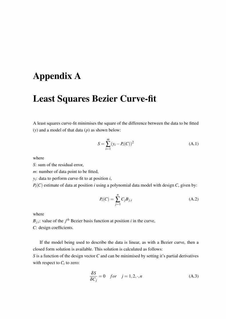
Appendix A
Least Squares Bezier Curve-fit
A least squares curve-fit minimises the square of the difference between the data to be fitted(y) and a model of that data (p) as shown below:
S =m
∑i=1
(yi −Pi(C))2 (A.1)
whereS: sum of the residual error,m: number of data point to be fitted,yi: data to perform curve-fit to at position i,Pi(C) estimate of data at position i using a polynomial data model with design C, given by:
Pi(C) =n
∑j=1
C jB j,i (A.2)
whereB j,i: value of the jth Bezier basis function at position i in the curve,C: design coefficients.
If the model being used to describe the data is linear, as with a Bezier curve, then aclosed form solution is available. This solution is calculated as follows:S is a function of the design vector C and can be minimised by setting it’s partial derivativeswith respect to Ci to zero:
δSδC j
= 0 f or j = 1,2, ·,n (A.3)

180 Least Squares Bezier Curve-fit
now,
δSδC j
=δ
δC j(
m
∑i=1
(yactuali −
n
∑j=1
C jB j,i)2) = 2
m
∑i=1
(yactuali −
n
∑j=1
C jB j,i)(−Bi, j) (A.4)
Therefore the conditions for S being minimised can be written as:
δSδC j
=−2Bi, j
m
∑i=1
(yactuali −
n
∑j=1
C jB j,i) = 0 (A.5)
This can be re-arranged to give:(BT B)C = BTY (A.6)
Therefore the design vector that minimises the least squares difference between a Beziercurve and a given data set (y) can be calculated from:
C = (BT B)−1BTY (A.7)
Note that the term least squared(BT B)BT = Bls (A.8)
is fixed by the Bezier basis functions and the chosen resolution of the curve, therefore thisterm only needs to be calculated once, at the start of a simulation. The Bezier curve thatbest fits a given data set Y in a least squares sense can therefore be calculated on-line by asingle matrix-vector multiplication:
C = BlsY (A.9)

Appendix B
Summery of Extended Interviews andDiscussions with a Pilot
Extended interviews and discussions about the problem have been carried out with MrsSusan Szasz who is a pilot at National Flying Lab, Cranfield University. She was helpfulin giving her experience and advice that were useful in achieving this thesis. The followingtable summarises the topics that discussed in the sessions of the interviews.
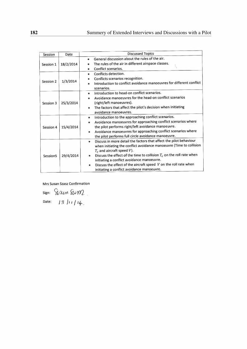
182 Summery of Extended Interviews and Discussions with a Pilot