collinearity and separated data in the … · 411 la colinealidad y la separaciÓn en los datos en...

411

LA COLINEALIDAD Y LA SEPARACIÓN EN LOS DATOS EN EL MODELO DE REGRESIÓN LOGÍSTICA

COLLINEARITY AND SEPARATED DATA IN THE LOGISTIC REGRESSION MODEL

Flaviano Godínez-Jaimes1*, Gustavo Ramírez-Valverde2, Ramón Reyes-Carreto1, F. Julian Ariza-Hernandez1, Elia Barrera-Rodriguez1

1Unidad Académica de Matemáticas, Universidad Autónoma de Guerrero. 39090. Chilpan-cingo, Guerrero. ([email protected]), ([email protected]), ([email protected]), ([email protected]). 2Estadística. Campus Montecillo. Colegio de Postgraduados. 56230. Montecillo, Estado de México. ([email protected]).

Resumen

La colinealidad y la falta de traslape en los datos son pro-blemas que afectan la inferencia basada en el modelo de re-gresión logística. Mediante simulación se investigó como son afectados los estimadores que tratan la colinealidad (Ridge iterativo), la separación en los datos (de Firth, y de Rous-seeuw y Christmann) o ambos problemas (de Shen y Gao). Estos estimadores se compararon considerando el número de condición escalado de la matriz de información estima-da, el sesgo y el error cuadrático medio. En cada uno de los cuatro escenarios estudiados, formados al usar dos niveles de colinealidad y dos tamaños de muestra, se consideraron tres grados de traslape en los datos. Se encontró que los estimado-res Ridge iterativo y de Shen y Gao tienen condicionamiento nulo, además el sesgo y el error cuadrático medio más peque-ños. El grado de traslape y el nivel de colinealidad afectan fuertemente el sesgo y el error cuadrático medio de los esti-madores de máxima verosimilitud, de Firth y de Rousseeuw y Christmann.

Palabras clave: estimador de Firth, estimador de máxima verosi-militud estimada, estimador doble penalizado, estimador Ridge iterativo, datos traslapados.

IntRoduccIón

Sean Yi, i=1,…n, variables aleatorias indepen-dientes con distribución Bernoulli con proba-bilidad de éxito pi = P(Yi = 1|xT

i ). Además, sea X la matriz diseño de orden n x (p+1) cuyos renglones son xT

i = (1, xi1, ..., xip), que corresponden a la i-ésima

* Autor responsable v Author for correspondence.Recibido: diciembre, 2011. Aprobado: abril, 2012.Publicado como ARTÍCULO en Agrociencia 46: 411-425. 2012.

AbstRAct

Collinearity and the lack of overlap in the data are problems that affect inference based on the logistic regression model. Simulation was used to investigate how the estimators that deal with collinearity (iterative Ridge) are affected, along with separation in the data (Firth’s, and Rousseeuw and Christmann’s) or both problems (Shen and Gao’s). These estimators were compared considering the scaled condition number of the estimated information matrix, the bias and the mean squared error. In each one of the four scenarios studied, formed by using two levels of collinearity and two sample sizes, three degrees of overlap were considered in the data. It was found that iterative Ridge and Shen and Gao’s estimators have null conditioning, as well as smaller bias and mean square error. The degree of overlap and the level of collinearity strongly affect the bias and mean square error of the maximum likelihood, Firth’s and Rousseeuw and Christmann’s estimators.

Key words: Firth’s estimator, estimated maximum likelihood estimator, penalized double estimator, iterative Ridge estimator, overlapped data.

IntRoductIon

Let Yi, i=1…n, be independent random variables with Bernoulli distribution with probability of success pi = P(Yi = 1|xT

i ). Furthermore, let X be the n x (p+1) design matrix whith rows xT

i = (1, xi1, ..., xip), which correspond to the i-th observation of the independent variables X1, ..., Xp. The logistic regression model assumes that the independent variables and the response variable are related by:

π β βi i i

T x xP Y x e eiT

iT

= = = +FH IK1 1e j

AGROCIENCIA, 16 de mayo - 30 de junio, 2012

VOLUMEN 46, NÚMERO 4412

observación de las variables independientes X1, ..., Xp. El modelo de regresión logística supone que las variables independientes y la variable respuesta están relacionadas por:

π β βi i i

T x xP Y x e eiT

iT

= = = +FH IK1 1e j

donde b=(b0, b1, ..., bp)T es el vector de parámetros

desconocido.

El estimador de máxima verosimilitud (MV), β se obtiene al maximizar la función de logverosimilitud:

l Y Yi i i ii

n( ) log logβ π π= + − −

=∑ b g b g b go t1 1

1

Bajo los supuestos de que X es de rango completo y b pertenece al interior del espacio de parámetros, β es la solución del sistema de p+1 ecuaciones for-

madas al igualar a cero las derivadas de l(b) respecto a b. El sistema de ecuaciones se resuelve usando méto-dos iterativos, como el método de Newton-Raphson, que está dado por:

b(s) = b(s) + I-1 (b(s)) U (b(s))

donde U(b) = XT (y-p(b)) es el vector de prime-ras derivadas parciales de l(b)

e I X VXTβb g =

es la matriz de información estimada con ,..., V diag n n= − −π π π π1 11 1b g b gm r .

Si la matriz I(b(s)) no tiene inversa entonces no existe el estimador de MV. Lesaffre y Marx (1993) demuestran que la matriz de información estimada del modelo de regresión logística es singular si: 1) X es de rango incompleto o 2) β se acerca a la frontera del espacio de parámetros.

Aun cuando X sea de rango completo pueden existir dependencias lineales cercanas entre sus co-lumnas, esto es, c0X0 +...+cpXp » 0 con c0,...,cp no to-das cero. Entre más cerca a cero esté la combinación lineal, más cerca está X a la singularidad, fenómeno conocido como colinealidad entre las variables inde-pendientes.

La colinealidad en regresión logística causa los siguientes problemas: 1) β es sensible a cambios

where b=(b0, b1, ..., bp)T is the unknown parameters

vector.

The maximum likelihood estimator (ML), β , is obtained by maximizing the loglikelihood function:

l Y Yi i i ii

n( ) log logβ π π= + − −

=∑ b g b g b go t1 1

1

Under the assumption that X is full rank and b belongs to the interior of the parameters space, β is the solution of the p+1 equations system formed by equaling to zero the derivates of l(b) with respect to b. The equations system is solved using iterative methods, such as the Newton-Raphson method, which is given by:

b(s) = b(s) + I-1 (b(s)) U (b(s))

where U(b) = XT (y-p(b)) is the first partial derivates vector of l(b) and I X VXT( ) β = is the information matrix estimated with ,..., V diag n n= − −π π π π1 11 1b g b gm r .

If the matrix I(b(s)) has no inverse then the ML estimator does not exist. Lesaffre and Marx (1993) prove that the estimated information matrix from the logistic regression model is singular if: 1) X is non full rank or 2) β approaches to the boundary of the parameters space.

Even when X is full rank there may exist near linear dependencies among its columns, that is, c0X0+...+cpXp » 0

with c0,...,cp

not all zero. The closer to zero the linear combination is, the closer X is to singularity, a phenomenon known as collinearity among the independent variables.

Collinearity in logistic regression causes the following problems: 1) β is sensitive to small changes in the independent variables, 2) some components of β are large and 3) the estimated variances of some

components of β are very large. As a consequence of these problems, the confidence intervals are very wide and the hypothesis tests related to the significance of the parameters have low power (Schaefer et al., 1984; Lee and Silvapulle, 1988; Marx and Smith, 1990).

If π i approaches one or zero, then the element i in the diagonal of V is zero and there is no inverse of the matrix I(b). For ˆiπ to approximate one or zero,

413GODÍNEZ-JAIMES et al.


pequeños en las variables independientes, 2) algunas componentes de β son grandes y 3) las varianzas estimadas de algunas componentes de β son muy grandes. Como consecuencia de estos problemas re-sultan intervalos de confianza muy amplios y baja potencia de las pruebas de hipótesis relacionadas con la significancia de los parámetros (Schaeffer et al., 1984; Lee y Silvapulle, 1988; Marx y Smith, 1990).

Si π i se aproxima a uno o a cero, entonces el elemento i en la diagonal de V es cero y no existe inversa de la matriz I(b). Para que ˆiπ se aproxime a uno o a cero, con xT

i fijo, debe ocurrir que al me-nos una β j → ±∞ , lo cual significa que β j está en la frontera del espacio de parámetros. Esto puede ocurrir cuando los datos tienen una configuración especial conocida como separación o casi separación. Albert y Anderson (1984) y Santner y Duffy (1986) demuestran que el estimador de MV del modelo de regresión logística no existe cuando hay separación o casi separación en los datos, y existe y es único cuan-do hay traslape en los datos.

Hay separación en los datos si existe un qÎRp-1 tal que, xT

i q>0 cuando Yi=1 y xTi q<0 cuando Yi=0,

para i=1,…,n. La casi separación en los datos ocu-rre si existe un qÎRp-1 \ {0} tal que xT

i q³0 cuando Yi=1 y xT

i q£0 cuando Yi=0, para todo i, y existe j Î{1,...,n} tal que xT

j q=0. Por último, existe traslape en los datos si no hay separación o casi separación en los datos. Si solamente hay una variable indepen-diente continua X y existe separación en los datos, entonces X es una variable predictiva perfecta, pues para alguna constante k, cuando X<k todos son éxi-tos y cuando X>k todos son fracasos o viceversa. Lo contradictorio es que en esta situación no existe esti-mador de MV del modelo de regresión logística.

En resumen, la matriz de información estimada, X VXT , se puede acercar a la singularidad por el efecto combinado de la colinealidad en las variables independientes, la cercanía a la separación en los da-tos o a que se presenten ambas condiciones.

Los estimadores Ridge en regresión logística son propuestos para reducir el tamaño de β ocasiona-do por la presencia de colinealidad. Schaefer et al. (1984) proponen un estimador Ridge logístico de un paso (RL) dado por:

( ) β βRT Tk X VX kI X VX= +

LNMM

OQPP

−1

with fixed xTi, must occur at least one β j → ±∞

which means that β j is at the boundary of the parameters space. This can occur when the data have a special configuration known as separation or quasi-separation. Albert and Anderson (1984) and Santner and Duffy (1986) prove that the ML estimator of the logistic regression model does not exist when there is separation or quasi-separation in the data, and it exists and is unique when there is overlap in the data.

There is separation in the data if there exists qÎRp-1 so that xT

i q>0 when Yi=1 and xTi q<0 when

Yi=0, for i= 1,…n. The quasi-separation in the data occurs if there is a qÎRp-1 \ {0} so that xT

i q³0 when Yi=1 and xT

i q£0 when Yi=0, for every i, and there exists j Î{1,...,n} so that xT

j q=0. Finally, there is overlap in the data if there is no separation or quasi-separation in the data. If there is only one continuous independent variable X and there is separation in the data, then X is a perfect predictive variable, because for a constant k, when X<k all are successes and when X>k, all are failures ore vice-versa. What is contradictory is that in this situation there is no ML estimator of the logistic regression model.

In summary, the estimated information matrix, X VXT , can approach to singularity from the combined effect of collinearity in the independent variables, the proximity to separation in the data or both situations are present.

The Ridge estimators in logistic regression are proposed to reduce the size of β caused by the presence of collinearity. Schaefer et al. (1984) propose a one step logistic Ridge estimator (RL) given by:

( ) β βRT Tk X VX kI X VX= +

LNMM

OQPP

−1

le Cessie and van Houwenlingen (1992) propose a logistic iterative Ridge estimator which is obtained by maximizing the loglikelihood that is penalized with the square of the norm of b and where k is determined as a function of the estimator’s performance.

Schaefer et al. (1984) show for the one step Ridge estimator that it is always possible to find a value of k that produces an estimator with lower mean square error than that of the ML estimator. One problem with the Ridge estimator is that there is not exist a unique expression to determine k; some proposals



le Cessie y van Houwenlingen (1992) proponen un estimador Ridge iterativo logístico que se ob-tiene al maximizar la logverosimilitud que es pena-lizada con el cuadrado de la norma de b y donde k se determina en función del desempeño del es-timador.

Schaefer et al. (1984) muestran para el estimador Ridge de un paso que siempre es posible encontrar un valor de k que produce un estimador con me-nor error cuadrático medio que el del estimador de MV. Un problema con el estimador Ridge es que no existe una expresión única para determinar k; algu-nas propuestas son: 1/bTb, (p+1)/bTb

2, traza (XTVX)

/ bTXTVXb, 12

max vjTβe j donde vT

j es un vector propio de X VXT (Schaefer et al., 1984; Lee y Sil-vapulle, 1988; le Cessie y van Houwelingen, 1992). Para calcular k es necesario conocer b por lo que β se usa en su lugar; como consecuencia, el estimador RL herede los problemas del estimador de MV. Una forma de determinar el parámetro de Ridge, inde-pendiente de β , es k=(l1-100lp)/99, donde l1 y lp son los valores propios mayor y menor de XTX (Liu, 2003).

Firth (1993) propone un estimador para redu-cir el sesgo al usar muestras pequeñas en el mode-lo lineal generalizado. Heinze y Schemper (2002) muestran que ese estimador también existe cuando hay separación en los datos. Rousseeuw y Christ-mann (2003) proponen otro estimador cuando hay separación en los datos. Shen y Gao (2008) presentan un estimador para resolver los proble-mas de colinealidad y separación en los datos si-multáneamente.

Aunque Shen y Gao (2008) proponen su estima-dor para tratar con la colinealidad en las variables independientes y separación en los datos, la simu-lación que realizan induce separación en los datos pero no induce colinealidad. Además, los estimado-res Ridge se han propuesto para atenuar los efectos de la colinealidad, pero no han sido evaluados en presencia de separación de los datos, además de que en todos los casos tampoco se ha evaluado el condi-cionamiento del estimador. En esta investigación se utiliza simulación para estudiar el efecto del nivel de colinealidad y el grado de traslape en los estimado-res propuestos para 1) tratar la colinealidad (Ridge iterativo), 2) la separación en los datos (de Firth, y de Rousseeuw y Christmann) o 3) ambos problemas (de Shen y Gao).

are: 1/bTb, (p+1)/bTb2, traza (XTVX) / bTXTVXb,

12

max vjTβe j where vT

j is an eigenvector of X VXT (Schaefer et al., 1984; Lee and Silvapulle, 1988; le Cessie and van Houwelingen, 1992). To calculate k it is necessary to know b, thus β is used instead; as a consequence is that the RL estimator inherits the problems of the ML estimator. One form of determining the Ridge parameter, independently of β , is k=(l1-100lp)/99, where l1 and lp are the largest and smallest eigenvalues of XTX (Liu, 2003).

Firth (1993) proposes an estimator to reduce the bias by using small samples in the generalized linear model. Heinze and Schemper (2002) show that this estimator also exists when there is separation in the data. Rousseeuw and Christmann (2003) propose another estimator when there is separation in the data. Shen and Gao (2008) propose an estimator to solve the problems of collinearity and separation in the data simultaneously.

Although Shen and Gao (2008) propose their estimator to deal with collinearity in the independent variables and separation in the data, the simulation that they carry out induces separation in the data but does not induce collinearity. Furthermore, the Ridge estimators have been proposed to attenuate the effects of collinearity, but they have not been evaluated in the presence of separated data, in addition to the fact that in all of the cases the estimator conditioning has not been evaluated. In this research simulation is used to study the effect of the level of collinearity and the degree of overlap in the estimators proposed for 1) treating collinearity (iterative Ridge), 2) separated data ( Firth’s, and Rousseeuw and Christmann’s) or 3) both problems (Shen and Gao’s).

mAteRIAls And methods

Studied estimators

Iterative Ridge estimator

This estimator was proposed by le Cessie and van Houwenlingen (1992) penalizing the loglikelihood with the square of the norm of b. The loglikelihood function is:

l l kRI ( ) ( )β β β= − 2

where l(b) is the loglikelihood of the logistic regression model and k is the Ridge parameter. The logistic iterative Ridge estimator,



mAteRIAles y métodos

Estimadores estudiados

Estimador Ridge iterativo

Este estimador fue propuesto por le Cessie y van Houwenlin-gen (1992) penalizando la logverosimilitud con el cuadrado de la norma de b. La función de logverosimilitud es:

l l kRI ( ) ( )β β β= − 2

donde l(b) es la logverosimilitud del modelo de regresión logísti-ca y k

es el parámetro de Ridge. El estimador Ridge iterativo lo-

gístico, β RI , se obtiene usando el método de Newton-Raphson:

β β β β βRIs

RIs T

RIs

RIs

RIsX V X kI U k( ) ( ) ( ) ( ) ( )+

−= + + −1

12 2e j{ } e j{ }

donde k se obtiene minimizando la media de una medida del error de predicción como el error de clasificación, el cuadrado del error o menos la logverosimilitud. En el presente estudio el pa-rámetro Ridge se determina usando la propuesta de Liu (2003), k=(l1-100lp)/99.

Estimador de Firth

Este estimador puede considerarse como un estimador pena-lizado donde la función de penalización es la a priori invariante de Jeffreys. La función de logverosimilitud es:

l l IF β β βb g b g b g= +1

2log

donde I(b) es la matriz de información estimada del modelo de regresión logística. Las primeras derivadas parciales de lF(b) res-pecto a br igualadas a cero son:

U y h xFr i i i i ir

i

nβ π πb g b gn s= − + − =

=∑ 1 2 0

1/ (r=0,...,p)

hi es el i-ésimo elemento en la diagonal de

H V X X V X X VFT

FT

F=−

/ /1 2 1 1 2e j , donde V VF F= βe j . El esti-

mador de Firth, βF , se obtiene de manera iterativa usando el método de Newton-Raphson

β β βFs

Fs T

FF

FsX V X U

+ −= +1 1b g e j e j( ) ( )

β RI , is obtained using the Newton-Raphson method:

β β β β βRIs

RIs T

RIs

RIs

RIsX V X kI U k( ) ( ) ( ) ( ) ( )+

−= + + −1

12 2e j{ } e j{ }

where k is obtained by minimizing the mean of a measurement of the prediction error as the classification error, the square of the error or minus the loglikelihood. In the present study the Ridge parameter is determined using the proposal of Liu (2003), k=(l1-100lp)/99.

Firth’s estimator

This estimator can be considered as a penalized estimator where the penalty function is the Jeffreys invariant prior. The loglikelihood function is:

l l IF β β βb g b g b g= +1

2log

where I(b) is the estimated information matrix of the logistic regression model. The first partial derivates of lF(b) with respect to br equaled to zero are:

U y h xFr i i i i ir

i

nβ π πb g b gn s= − + − =

=∑ 1 2 0

1/ (r=0,...,p)

hi is the i-th element in the diagonal of

H V X X V X X VFT

FT

F=−

/ /1 2 1 1 2e j , where V VF F= βe j . The

Firth’s estimator, βF , is obtained iteratively using the Newton-Raphson method

β β βFs

Fs T

FF

FsX V X U

+ −= +1 1b g e j e j( ) ( )

Rousseeuw and Christmann’s estimator

Rousseeuw and Christmann (2003) propose a modification of the logistic regression model, which they name hidden logistic regression model. In this model it is assumed that the true status T, with values success (s) and failure (f), that cannot be observed due to an additional stochastic mechanism, but there is an observed binary variable Y that is strongly related to T. If the true status is T=s, Y=1 is observed with P(Y=1|T=s)=d1, therefore, a misclassification occurs with P(Y=0|T=s)=1-d1. Analogously, if the true status is T=f, Y=0 is observed with P(Y=0|T=f)=1-d0 and a misclassification with P(Y=1|T=f)=d0. If the probability of observing the true status is greater than 0.5, then 0< d0 <0.5<



Estimador de Rousseeuw y Christmann

Rousseeuw y Christmann (2003) proponen una modifica-ción del modelo de regresión logística al que denominan mo-delo de regresión logística escondido. En este modelo se supone que el verdadero status T, con valores éxito (s) y falla (f), no se puede observar debido a un mecanismo estocástico adicional, pero existe una variable binaria observada Y fuertemente rela-cionada con T. Si el verdadero status es T=s, se observa Y=1 con P(Y=1|T=s)=d1, por tanto, una clasificación incorrecta con P(Y=0|T=s)=1-d1. Análogamente, si el verdadero status es T=f se observa Y=0 con P(Y=0|T=f)=1-d0 y una clasificación in-correcta con P(Y=1|T=f)=d0. Si la probabilidad de observar el verdadero status es mayor a 0.5, entonces, 0< d0 <0.5< d1<1. El estimador de Rousseeuw y Christmann, β RC , se obtiene después de estimar la verosimilitud pues depende de d0 y d1

por lo cual los autores lo llaman estimador de máxima verosi-militud estimada. Este estimador se obtiene con el siguiente algoritmo:

1. Calcular max ,min , ,π δ δ π= −1b gd i donde

π ==∑

1

1nyi

i

n

y d=0.01.

2. Calcular δδπδ

δδπδ

δ δ0 1 0 11

1

11=

−=

+−

≠ −

,y .

3. Calcular las pseudo-observaciones ~Y Y Yi i i= − +1 0 1b gδ δ .

4. Ajustar el modelo de regresión logística en el cual se sustituyen las observaciones por las pseudo-observaciones.

Estimador de Shen y Gao

Para resolver simultáneamente los problemas de colinealidad y separación en los datos ellos usan una doble penalización de la logverosimilitud, una de tipo a priori no informativa de Jefreys y otra de tipo Ridge dada por el cuadrado de la norma de b, esto es:

l l ISG β β β λ βb g b g= + −1

22

log ( )

El estimador de Shen y Gao, βSG , se obtiene usando el mé-todo de Newton-Raphson donde el parámetro l se obtiene mi-nimizando, mediante validación cruzada, la media del cuadrado

del error, MCEn

Y

hVC

i i

iii

nλ

πλ

b g e jb g

=−

−=∑

1

1

2

21

.

d1<1. The estimator of Rousseeuw and Christmann, β RC , is obtained after estimating the likelihood, as it depends on d0 and d1, for which the authors call it the estimated maximum likelihood estimator. This estimator is obtained with the following algorithm:

1. Calculate max ,min , ,π δ δ π= −1b gd i , where

π ==∑

1

1nyi

i

n

and d=0.01.

2. Calculate δδπδ

δδπδ

δ δ0 1 0 11

1

11=

−=

+−

≠ −

,y .

3. Calculate the pseudo-observations ~Y Y Yi i i= − +1 0 1b gδ δ .

4. Fit the logistic regression model in which the observations are substituted for the pseudo-observations.

Estimator of Shen and Gao

To simultaneously solve the problems of collinearity and separation in the data, they use a double penalization of the loglikelihood, one Jeffreys non-informative prior and the other of Ridge type given by the square of the norm of b, that is:

l l ISG β β β λ βb g b g= + −1

22

log ( )

The estimator of Shen and Gao, βSG , is obtained by using the Newton-Raphson method where the parameter l is obtained by minimizing, using cross validation, the mean squared error,

MCEn

Y

hVC

i i

iii

nλ

πλ

b g e jb g

=−

−=∑

1

1

2

21

.

Diagnostic

Belsley and Oldford (1986) studied the behavior of the system of equations y=f(w) with small changes in w and they called it conditioning analysis. If y has big changes when w has small changes, it is said that y is ill conditioned. They identify three types of conditioning: of the data, of the estimator and of the criterion.

Data conditioning. In logistic regression data conditioning is related with the collinearity in the independent variables and is diagnosed with the scaled condition number of the design matrix proposed by Belsey et al. (1980). The scaled condition number



Diagnóstico

Belsley y Oldford (1986) estudiaron el comportamiento del sistema de ecuaciones y=f(w) ante pequeños cambios en w y lo llamaron análisis de condicionamiento. Si y tiene cambios gran-des cuando w tiene cambios pequeños se dice que y está mal condicionado. Ellos identifican tres tipos de condicionamiento: de los datos, del estimador y del criterio.

Condicionamiento de los datos. En regresión logística el con-dicionamiento de los datos está relacionado con la colinealidad en las variables independientes y se diagnostica con el número de condición escalado de la matriz diseño propuesto por Belsley et al. (1980). El número de condición escalado de X se define

por η λ λx p= +1 1* * donde l*

1 y l*p+1 son el máximo y el mí-

nimo de los valores propios de XTX después de ser escalada. La colinealidad está presente en cualquier conjunto de variables in-dependientes, pero no siempre afecta de manera importante la estimación o inferencia. Belsley et al. (1980) clasifican la colinea-lidad en tres niveles de acuerdo a su intensidad: 1) nula (hx<10), 2) moderada (10£hx<30) y 3) severa (hx<30).

Condicionamiento del estimador. El diagnóstico se realiza con el número de condición escalado de la matriz de información

estimada, que se define por η λ λMI p= +1 1** ** , donde l

1** y

l**p+1 son los valores propios máximo y mínimo de la matriz de

información estimada escalada. El nivel de condicionamiento de esta matriz medido por hMI se determina de forma similar a hx.

Condicionamiento del criterio. β se obtiene maximizando la verosimilitud, Belsley y Oldford (1986) afirman que hMI permite valorar este tipo de condicionamiento. Por esta razón no se con-sidera en el presente estudio.

El condicionamiento de los estimadores de MV, de Fir-th, de Rousseeuw y Christmann, de Shen y Gao y Rid-ge iterativo se miden en las matrices de información esti-madas: X VXT , X V XT

F , X V XT

RC , X V X IT

SG − 2λ y

X V X kITRI + 2 . El estimador de Firth se obtiene usando el pa-

quete logistf (Ploner et al., 2010) de R Development Core Team, 2011, y el estimador de Rousseeuw y Christmann con el paquete hlr de R (Rousseeuw y Christmann, 2008).

Separación de los datos

La detección de la separación en los datos fue analizada por Santner y Duffy (1986) usando un procedimiento basado en programación lineal, el cual no fue implementado en los pa-quetes estadísticos. En SAS se advierte al usuario cuando puede

of X is defined by η λ λx p= +1 1* *

where l

*1 and l*

p+1 are the maximum and the minimum of the eigenvalues of XTX after being scaled. Collinearity is present in any set of independent variables, but does not always have an important effect on the estimation or inference. Belsely et al. (1980) classify collinearity in three levels according to its intensity: 1) null (hx<10), 2) moderate (10£hx<30) and 3) severe (hx<30).

Estimator conditioning. The diagnostic is done with the scaled condition number of the estimated information matrix, which

is defined by η λ λMI p= +1 1** ** , where l

1** and l**

p+1 are the maximum and minimum eigenvalues of the scaled estimated information matrix. The conditioning level of this matrix measured by hMI

is determined in a similar form to hx.

Criterion conditioning. β is obtained by maximizing the likelihood, and Belsely and Oldford (1986) affirm that hMI makes it possible to asses this type of conditioning. For this reason it is not considered in the present study.

The conditioning of the ML, Firth’s, Rousseeuw and Christmann’s, Shen and Gao’s and iterative Ridge estimators are measured in the estimated information matrix: X VXT , X V XT

F , X V XT

RC , X V X IT

SG − 2λ and X V X kIT

RI + 2 .

The Firth’s estimator is obtained using the de R (R Development Core Team, 2011) logistf package (Ploner et al., 2010), and the Rousseeuw and Christmann’s estimator with the R hlr package (Rousseeuw and Christmann, 2008).

Separation of the data

The detection of the separation in the data was analyzed by Santner and Duffy (1986) using a procedure based on linear programming which was not implemented in statistical packages. In SAS the user is warned when there may be separation or quasi-separation in the data but the algorithm used is not accurate. Rousseeuw and Christmann (2004) propose a procedure based on regression depth and implemented in the noverlap package of R. This procedure is used in the present study and determines the number of observations to eliminate for there to be separation in the data. Konis (2009) proposes a procedure based on quadratic programming implemented in the safeBinaryRegression package of R; however, this procedure is not used because when separation is identified in the data, it automatically declares the non-existence of the ML estimator.

Simulation study

The simulation study consisted of carrying out 1500 replicates in each one of the scenarios generated by the combinations of the two factors studied: collinearity and sample size.



haber separación o casi separación en los datos pero el algoritmo usado no es preciso. Rousseeuw y Christmann (2004) proponen un procedimiento basado en regresión profunda e implementado en el paquete noverlap (Rousseeuw and Christmann, 2004) de R. Este procedimiento se usa en el presente estudio y determina el número de observaciones a eliminar para que haya separación en los datos. Konis (2009) propone un procedimiento basado en programación cuadrática implementado en el paquete safeBi-naryRegresion de R; sin embargo, este procedimiento no se usa porque al identificar separación en los datos automáticamente declara la no existencia del estimador de MV.

Estudio de simulación

El estudio de simulación consistió en realizar 1500 repeti-ciones en cada uno de los escenarios generados por las combi-naciones de los dos factores estudiados: colinealidad y tamaño de muestra.

Colinealidad entre las variables independientes (C). Se usa-ron dos grados de colinealidad: 1) moderada (hx=16) y 2) severa (hx=32).

Tamaño de muestra (TM). Se consideraron dos tamaños de muestra 20 y 40.

Grado de traslape (GT). Se consideraron cuatro grados de tras-lape que se construyeron después de generar los datos, clasifi-cando cada caso en los grupos G0, G1, G2 y G3 de acuerdo a si las proporciones de observaciones traslapadas, detectadas con el paquete noverlap, están en los intervalos [0, 0.025], (0.025, 0.125], (0.125, 0.225] y (0.225, 0.325] respectivamente. El aná-lisis considera solamente los primeros tres grupos porque no en todos los escenarios se obtuvieron los cuatro grupos.

Generación de los datos

Variables independientes

Se usaron dos variables independientes que se construyeron usando dos variables con distribución uniforme en [0,1], X1 y W; la variable X1 fue la primer variable independientes y la segunda se construyó con X2=X1+cW, donde c toma valores apropiados para obtener los números de condición escalados hx=16 y hx=32.

Variable respuesta

Se obtuvo con Yi=1 si pi>Ui y Yi=0 en otro caso;

i=1,…, n; donde Ui tiene distribución uniforme en [0, 1] y

Collinearity among the independent variables (C). Two degrees of collinearity were used: 1) moderate (hx=16) and 2) severe (hx=32).

Sample size (TM). Two sample sizes were considered, 20 and 40.

Degree of overlap (GT). Four degrees of overlap were considered, which were constructed after generating the data, classifying each case in the groups G0, G1, G2 and G3 according to whether the proportions of overlapped observations, detected with the program noverlap, are in the intervals [0, 0.025], (0.025, 0.125], (0.125, 0.225] and (0.225, 0.325] respectively. The analysis only considers the first three groups because the four groups were not obtained in all of the scenarios.

Generation of the data

Independent variables

Two independent variables were used that were constructed using two variables with uniform distribution in [0, 1], X1

and W; the variable X1 was the first independent variable, and the second was constructed with X2=X1+cW, where c takes appropriate values for obtaining the scaled condition numbers hx=16

and hx=32.

Response variable

This was obtained with Yi=1 if pi>Ui

and Yi=0 in another

case; i=1,…, n; where Ui has uniform distribution in [0, 1] and

π β βi

x xe eiT

iT

= +FHG

IKJ1 where b is two times the eigenvector

associated to the maximum eigenvalue of XTX.

Comparison of estimators

This was carried out as a function of :

1. he scaled condition number of the estimated information matrix: hMI.

2. The mean square error: ECMRi ri i

r

R~ ~β β βe j e j= −

=∑

1 2

1

.

3. The bias: BRi ri i

r


=∑

1

1.

where ~β i

is one of the estimators of bi in the r-th repetition.



π β βi

x xe eiT

iT

= +FHG

IKJ1 donde b es dos veces el vector propio

asociado al valor propio mayor de XTX.

Comparación de estimadores

Se realizó en función de:

1. El número de condición escalado de la matriz de información estimada: hMI.

2. El error cuadrático medio: ECMRi ri i

r


=∑

1 2

1.

3. El sesgo: BRi ri i

r


=∑

1

1

donde ~β i es uno de los estimadores de bi en la r-ésima repeti-

ción.

ResultAdos y dIscusIón

Se usan los términos estimadores originales para aludir a los estimadores de MV, de Firth (F), de Rousseeuw y Christmann (RC) y estimadores Ridge para referirse a los estimadores de Shen y Gao (SG) y Ridge iterativo (RI).

Efecto en el condicionamiento del estimador

Los estimadores originales fueron muy sensibles a la colinealidad y al grado de traslape estudiados, ya que presentaron un condicionamiento severo de la matriz de información para cualquier tamaño de muestra, niveles de colinealidad y grado de traslape estudiados (Cuadro 1).

También se observó, como se esperaba, que el nú-mero de condición escalado de los estimadores ori-ginales fue mayor cuando existe colinealidad severa, que en moderada o con TM 20, que con TM 40 y con grados de traslape bajos. Los estimadores RI y de SG presentaron condicionamiento nulo.

Efecto en el error cuadrático medio

Los estimadores originales tuvieron mayor ECM que los estimadores Ridge (Cuadro 2), lo cual es de esperarse ya que los estimadores Ridge surgieron con el fin de reducir el ECM (Schaefer et al., 1984).

Cuadro 1. Números de condición escalados de la matriz de información estimada escalada de los estimado-res.

Table 1. Scaled condition numbers of the scaled estimated information matrix of the estimators.

TM GT C MV F RC SG RI

40 G0 S 1739634 1474 63743 1 4 G1 1396 1198 1364 1 5 G2 1181 1195 1182 1 7 G0 M 35403 345 6109 1 4 G1 350 281 342 1 6 G2 263 269 263 1 9 G0 S 83071 5050 71064 1 4 G1 16857 3600 9511 1 520 G2 3666 3419 3651 1 7 G0 M 1224672 635 259001 1 5 G1 3156 521 1880 1 6 G2 496 483 495 1 9

Results And dIscussIon

The terms original estimators are used to allude to the ML, Firth’s (F), Rousseeuw and Christmann’s (RC) estimators and Ridge estimators to refer to the estimators Shen and Gao’s (SG) and iterative Ridge (RI).

Effect on the conditioning estimator

The original estimators were highly sensitive to collinearity and to the degree of overlap studied, given that they presented a severe conditioning of the estimated information matrix for any sample size, levels of collinearity and degree of overlap studied (Table 1).

It was also observed, as was expected, that the scaled condition number of the original estimators was higher when there is severe collinearity than in moderate or with TM 20, than with TM 40 and with low degrees of overlap. The estimators RI and SG presented null conditioning.

Effect on the mean square error

The original estimators had higher MSE than the Ridge estimators (Table 2), which is to be expected, since the Ridge estimators appeared with the purpose of reducing the MSE (Schaefer et al., 1984).

All of the estimators studied had the highest MSE



Todos los estimadores estudiados tuvieron el ma-yor ECM en G0 donde hay separación o casi separa-ción en los datos. Al aumentar el grado de traslape se observó una notable disminución en el ECM de los estimadores originales. El comportamiento del ECM es diferente en los estimadores Ridge pues en ellos el ECM es aproximadamente igual, como en SG, o incrementa, como en RI.

El efecto de la colinealidad fue muy fuerte en el ECM de los estimadores originales lo cual fue re-portado por Schaefer et al. (1984), le Cessie y van Houwenlingen (1992), Lee y Silvapulle (1988), Weissfeld y Sereika (1991) y Månsson y Shukur (2011). En colinealidad severa el ECM fue 2 a 150 veces mayor que en colinealidad moderada, con

Cuadro 2. Error cuadrático medio de los estimadores.Table 2. Mean squared error of the estimators.

EstimadoresTM GT C β i MV F RC SG RI

β1 233605000.00 452.15 41529.72 0.96 0.06 G0 S β2

215063500.00 420.82 39804.42 1.34 0.05 β1

1547933.37 80.60 4746.51 1.71 0.06 M β2

1432173.55 74.93 4924.40 2.00 0.06 β1

351.26 151.79 325.02 0.83 0.1040 G1 S β2

331.15 146.24 309.11 1.00 0.11 β1

78.05 30.63 71.46 2.04 0.10 M β2

67.91 25.78 62.99 1.86 0.13 β1

81.51 60.36 79.59 0.51 0.19 G2 S β2

80.34 59.46 78.45 0.87 0.23 β1

9.16 6.68 8.94 0.90 0.13 M β2

8.49 6.38 8.31 1.19 0.24 β1

14244771.30 2307.40 231184.98 1.01 0.13 G0 S β2

13311902.08 2060.56 216506.41 1.22 0.12 β1

167516819.58 212.61 86333.46 0.71 0.06 M β2

154311200.00 214.34 83470.89 1.04 0.05 β1

4691.48 575.43 3855.37 0.74 0.1320 G1 S β2

4470.82 533.48 3650.35 0.81 0.14 β1

793.62 54.33 421.49 0.78 0.15 M β2

823.11 60.00 429.61 1.45 0.16 β1

643.85 327.52 621.82 0.53 0.20 G2 S β2

570.80 295.28 551.66 0.52 0.23 β1

45.51 24.13 44.15 0.81 0.24 M β2

45.20 24.99 43.86 1.29 0.35

in G0 where there is separation or quasi-separation in the data. As the degree of overlap increased a notable reduction was observed in the MSE of the original estimators. The behavior of the MSE is different in the Ridge estimators, as the MSE in them is approximately equal, as in SG, or increases, as in RI.

The effect of collinearity was very strong in the MSE of the original estimators, which was reported by Schaefer et al. (1984), Lee and Silvapulle (1988), Weissfeld and Sereika (1991), le Cessie and van Houwenlingen (1992) and Månsson and Shukur (2011). In severe collinearity the MSE was 2 to 150 times higher than in moderate collinearity, with the exception of ML and RC in the G0 and TM 20. In the Ridge estimators the observed effect was the



excepción de los estimadores de MV y RC en el G0 y TM 20. En los estimadores Ridge el efecto observado fue al revés; en general; el ECM fue mayor en coli-nealidad moderada que en colinealidad severa.

En general, el ECM de los estimadores originales fue afectado de forma severa por el tamaño de mues-tra ya que su valor fue 2.64 a 130.58 veces más gran-de en TM 20 que en TM 40. Aunque también los estimadores Ridge tuvieron mayor ECM con TM 20 que en TM 40, esto fue menos frecuente y el incre-mento fue menor.

Entre los estimadores originales tuvo mejor desempeño el estimador F, aún en G0 donde hay separación y casi separación, y el estimador de peor

Cuadro 3. Sesgo de los estimadores estudiados.Table 3. Bias of the estimators studied.

EstimadoresTM GT C β i MV F RC SG RI

β1 -928.41 -2.01 -9.45 -0.12 -0.13

G0 S β2 1450.15 2.61 14.85 0.07 -0.12

β1 70.46 -0.46 5.77 -0.23 -0.15

M β2 35.65 0.54 2.68 -0.10 -0.15

β1 1.26 0.18 1.15 -0.20 -0.23

40 G1 S β2 -0.79 -0.32 -0.74 -0.24 -0.25

β1 -0.19 -0.23 -0.21 -0.24 -0.22

M β2 0.72 0.05 0.66 -0.27 -0.28

β1 -0.37 -0.59 -0.38 -0.33 -0.38

G2 S β2 -0.13 -0.09 -0.13 -0.52 -0.42

β1 0.29 0.10 0.28 -0.25 -0.33

M β2 -0.60 -0.61 -0.61 -0.54 -0.46

β1 -699.99 -0.53 -107.32 -0.22 0.00

G0 S β2 799.98 1.39 116.22 0.01 -0.01

β1 -4223.99 -0.19 -25.93 -0.09 -0.04

M β2 4661.87 1.90 62.08 -0.37 -0.07

β1 -6.71 1.37 -6.30 -0.40 -0.21

20 G1 S β2 5.91 -1.76 5.54 -0.34 -0.23

β1 -1.12 0.03 -0.41 -0.38 -0.26

M β2 2.17 -0.71 1.35 -0.68 -0.32

β1 0.41 1.45 0.40 -0.38 -0.34

G2 S β2 -0.79 -1.94 -0.80 -0.45 -0.39

β1 0.09 0.08 0.08 -0.35 -0.38

M β2 -0.37 -0.94 -0.38 -0.77 -0.53

opposite; in general, the MSE was higher in moderate than in severe collinearity.

In general, the MSE of the original estimators was affected severely by the sample size, given that its value was 2.64 to 130.58 times larger in TM 20 than in TM 40. Although the Ridge estimators also had higher MSE with TM 20 than in TM 40, it was less frequent and the increment was lower.

Among the original estimators, the F estimator had a better performance, even in G0 where there is separation and quasi-separation, and the ML estimator had the worst performance. In the Ridge estimators, the RI had the lowest MSE followed by the SG estimator.



desempeño fue el de MV. En los estimadores Ridge, el RI tuvo el menor ECM seguido del estimador de SG.

Efecto en el sesgo

Los estimadores originales tuvieron mayor sesgo que los estimadores Ridge en los tres grados de tras-lape al usar TM de 20, pero con TM 40 solamente ocurrió en G0 (Cuadro 3). Los estimadores originales tuvieron mayor sesgo en G0, donde hay separación o casi separación en los datos, y disminuyó en G1 y G2. Por el contrario, los estimadores Ridge gene-ralmente tuvieron menor sesgo en G0 y al aumentar el porcentaje de traslape incrementó ligeramente el sesgo.

El efecto de la colinealidad fue fuerte en el sesgo de los estimadores originales. El mayor sesgo se obtu-vo en colinealidad severa y disminuyó al incrementar el grado de traslape. En los estimadores Ridge se ob-servó un comportamiento opuesto, pues en general fue mayor el sesgo en colinealidad moderada que en colinealidad severa. Es interesante notar que en los estimadores Ridge el sesgo, aunque pequeño, siem-pre fue negativo.

Schaefer (1983) y Ramírez-Valverde y Rice (1995) muestran que el sesgo de β es aproximadamente

B X VX X V x X VX xT Tk k

T Tk

β πe j e j b g e j= − −RST

UVW− −1

21 2

1 1

por lo cual el sesgo del estimador de MV es afectado por ambos problemas, el de colinealidad en las varia-bles independientes (matriz X) y el de la cercanía a la separación (matriz V).

Ramírez-Valverde y Rice (1995), aunque sola-mente estudiaron el efecto de la colinealidad, tam-bién muestran que el sesgo del estimador de MV es mayor que el sesgo del estimador Ridge de un paso. En la literatura revisada, no se encontraron investi-gaciones acerca del efecto del grado de traslape en el sesgo de los estimadores evaluados en el presente estudio.

El TM afectó fuertemente el sesgo de los estima-dores originales. El sesgo en valor absoluto fue, gene-ralmente, entre 1.05 y 130.77 veces mayor con TM 20 que con TM 40. Por el contrario, los estimadores Ridge tuvieron mayor sesgo con TM 40 que con TM 20. Entre los estimadores originales el estimador F

Effect on the bias

The original estimators had greater bias than the Ridge estimators in the three degrees of overlap using TM of 20, but with TM 40 it only occurred in G0 (Table 3). The original estimators had greater bias in G0, where there is separation or quasi-separation in the data, and it decreased in G1 and G2. In contrast, the Ridge estimators generally had lower bias in G0 and as the percentage of overlap increased the bias increased slightly.

The effect of collinearity was strong in the bias of the original estimators. The greatest bias was obtained in severe collineariity and decreased as the degree of overlap increased. In the Ridge estimators the opposite behavior was observed, as in general the bias was greater in moderate collinearity than in severe collinearity. It is interesting to note that in the Ridge estimators, the bias, although small, was always negative. Schaefer (1983) and Ramírez-Valverde and Rice (1995) show that the bias of β is approximately

B X VX X V x X VX xT Tk k

T Tk

β πe j e j b g e j= − −RST

UVW− −1

21 2

1 1

therefore, the bias of the ML estimator is affected by both problems, that of collinearity in the independent variables (matrix X) and that of proximity to separation (matrix V).

Ramírez-Valverde and Rice (1995), although they only studied the effect of collinearity, also show that the bias of the ML estimator is higher than the bias of the one step Ridge estimator. In the revised literature, no investigations were found of the effect of the degree of overlap in the bias of the estimators evaluated in the present study.

The TM strongly affected the bias of the original estimators. The bias in absolute value was, generally, 1.05 to 130.77 times higher with TM 20 than with TM 40. In contrast, the Ridge estimators had higher bias with TM 40 than with TM 20. Among the original estimators the F estimator had the best performance, even in the G0 where there is less overlap, while the ML estimator was notoriously bad. The estimators RI and SG had the lowest bias among the Ridge estimators, especially the first. The Ridge estimators in logistic regression, in contrast to the Ridge estimators in linear regression, present less bias than the ML estimator.



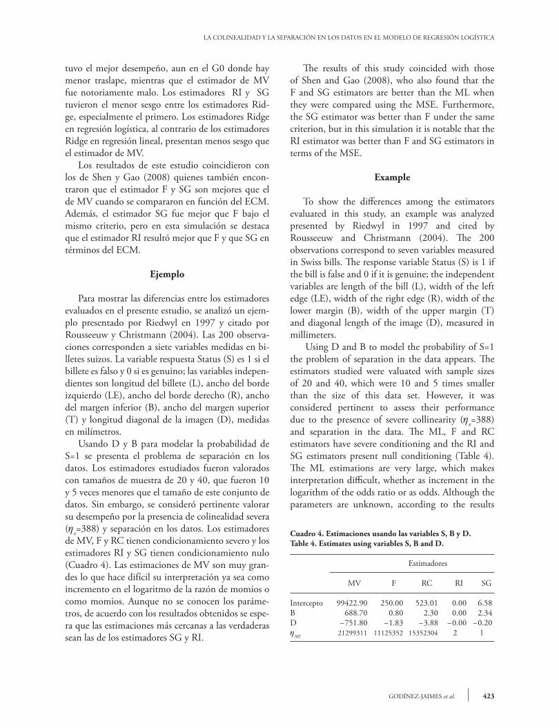
Cuadro 4. Estimaciones usando las variables S, B y D.Table 4. Estimates using variables S, B and D.

Estimadores

MV F RC RI SG

Intercepto 99422.90 250.00 523.01 0.00 6.58B 688.70 0.80 2.30 0.00 2.34 D -751.80 -1.83 -3.88 -0.00 -0.20hMI 21299311 11125352 15352304 2 1

tuvo el mejor desempeño, aun en el G0 donde hay menor traslape, mientras que el estimador de MV fue notoriamente malo. Los estimadores RI y SG tuvieron el menor sesgo entre los estimadores Rid-ge, especialmente el primero. Los estimadores Ridge en regresión logística, al contrario de los estimadores Ridge en regresión lineal, presentan menos sesgo que el estimador de MV.

Los resultados de este estudio coincidieron con los de Shen y Gao (2008) quienes también encon-traron que el estimador F y SG son mejores que el de MV cuando se compararon en función del ECM. Además, el estimador SG fue mejor que F bajo el mismo criterio, pero en esta simulación se destaca que el estimador RI resultó mejor que F y que SG en términos del ECM.

Ejemplo

Para mostrar las diferencias entre los estimadores evaluados en el presente estudio, se analizó un ejem-plo presentado por Riedwyl en 1997 y citado por Rousseeuw y Christmann (2004). Las 200 observa-ciones corresponden a siete variables medidas en bi-lletes suizos. La variable respuesta Status (S) es 1 si el billete es falso y 0 si es genuino; las variables indepen-dientes son longitud del billete (L), ancho del borde izquierdo (LE), ancho del borde derecho (R), ancho del margen inferior (B), ancho del margen superior (T) y longitud diagonal de la imagen (D), medidas en milímetros.

Usando D y B para modelar la probabilidad de S=1 se presenta el problema de separación en los datos. Los estimadores estudiados fueron valorados con tamaños de muestra de 20 y 40, que fueron 10 y 5 veces menores que el tamaño de este conjunto de datos. Sin embargo, se consideró pertinente valorar su desempeño por la presencia de colinealidad severa (hx=388) y separación en los datos. Los estimadores de MV, F y RC tienen condicionamiento severo y los estimadores RI y SG tienen condicionamiento nulo (Cuadro 4). Las estimaciones de MV son muy gran-des lo que hace difícil su interpretación ya sea como incremento en el logaritmo de la razón de momios o como momios. Aunque no se conocen los paráme-tros, de acuerdo con los resultados obtenidos se espe-ra que las estimaciones más cercanas a las verdaderas sean las de los estimadores SG y RI.

The results of this study coincided with those of Shen and Gao (2008), who also found that the F and SG estimators are better than the ML when they were compared using the MSE. Furthermore, the SG estimator was better than F under the same criterion, but in this simulation it is notable that the RI estimator was better than F and SG estimators in terms of the MSE.

Example

To show the differences among the estimators evaluated in this study, an example was analyzed presented by Riedwyl in 1997 and cited by Rousseeuw and Christmann (2004). The 200 observations correspond to seven variables measured in Swiss bills. The response variable Status (S) is 1 if the bill is false and 0 if it is genuine; the independent variables are length of the bill (L), width of the left edge (LE), width of the right edge (R), width of the lower margin (B), width of the upper margin (T) and diagonal length of the image (D), measured in millimeters. Using D and B to model the probability of S=1 the problem of separation in the data appears. The estimators studied were valuated with sample sizes of 20 and 40, which were 10 and 5 times smaller than the size of this data set. However, it was considered pertinent to assess their performance due to the presence of severe collinearity (hx=388) and separation in the data. The ML, F and RC estimators have severe conditioning and the RI and SG estimators present null conditioning (Table 4). The ML estimations are very large, which makes interpretation difficult, whether as increment in the logarithm of the odds ratio or as odds. Although the parameters are unknown, according to the results



conclusIones

Es una ventaja que los estimadores de Firth y de Rousseeuw y Christmann existan cuando hay separa-ción en los datos, pero son fuertemente afectados por el nivel de colinealidad entre las variables indepen-dientes y por bajos grados de traslape en los datos, efectos que son mayores cuando el tamaño de mues-tra es pequeño. Los estimadores Ridge iterativo y de Shen y Gao son mejores, en términos de error cua-drático medio y de sesgo, cuando se presentan simul-táneamente los problemas de colinealidad, poco tras-lape en los datos y el tamaño de muestra sea pequeño. Aunque las diferencias fueron pequeñas, el estimador Ridge iterativo tuvo un mejor comportamiento que el estimador de Shen y Gao.

Respecto a los estimadores Ridge iterativo y de Shen y Gao hace falta investigación para proponer intervalos de confianza de los parámetros estimados; así como considerar un número mayor de variables en las que haya más de una relación de colinealidad. También merece atención proponer formas para de-terminar el parámetro de Ridge que tomen en cuenta el nivel de colinealidad, el número de relaciones de colinealidad y el grado de traslape en los datos.

lIteRAtuRA cItAdA

Albert, A., and J. A. Anderson. 1984. On the existence of maxi-mum likelihood estimates in logistic regression models. Bio-metrika 71:1-10.

Belsley, D. A., E. Kuh, and R. Welsh. 1980. Regression Diagnos-tics: Identifying Influential Data and Source of Collinearity. John Wiley & Sons. New York. 393 p.

Belsley, D. A., and R. W. Oldford. 1986. The general problem of ill-conditioning in statistical analysis. Comput. Stat. Data An. 4:103-120.

Firth, D. 1993. Bias reduction of maximum likelihood estimates. Biometrika 80: 27-38.

Heinze, G., and M. Schemper. 2002. A solution to the problem of separation in logistic regression. Stat. Med. 21: 2409-2419.

Konis, K. 2009. safebinaryRegression. R package version 0.1-2. http://www.r-project.org (Consulta: julio, 2010).

le Cessie, S. and J. C. van Houwelingen. 1992. Ridge estimators in logistic regression. Appl. Statistics 41(1): 191-201.

Lee, A. H., and M. J. Silvapulle. 1988. Ridge estimation in logistic regression. Comm. in Statistics-Theory and Methods 17(4): 1231-1257.

Lesaffre, E., and B. D. Marx. 1993. Collinearity in generalized linear regression. Comm. Statistics-Theory and Methods 22(7):1933-1952.

Liu, K. 2003. Using Liu-type estimator to combat collinearity. Comm. Statistics-Theory and Methods 32(5): 1009-1020.

Månsson K., and G. Shukur. 2011. On ridge parameters in lo-gistic regression. Comm. Statistics - Theory and Methods 40(18): 3366-3381.

Marx, B. D., and E. P. Smith. 1990. Weighted multicollineari-ty in logistic regression: Diagnostics and biased estimation techniques with an example from lake acidification. Can. J. Fish. Aquat. Sci. 47: 1128-1135.

Ploner, M., D. Dunkler, H. Southworth, and G. Heinze. 2010. logistf: Firth’s bias reduced logistic regression. R package version 1.10. http://CRAN.R-project.org/package=logistf (Consulta: agosto, 2010).

R Development Core Team. 2011. R: A language and environ-ment for statistical computing. R Foundation for Statistical Computing, Vienna, Austria. ISBN 3-900051-07-0, URL http://www.R-project.org/ (Consulta: octubre, 2010).

Ramírez-Valverde, G., and J. C. Rice. 1995. Bias and collinea-rity in logistic regression. ASA Proc. Epidemiology Section 97-101.

obtained it is expected that the estimations closest to the true ones are those of the SG and RI estimators.

conclusIons

It is an advantage that the Firth’s and Rousseeuw and Christmann’s estimators exist when there is separation in the data, but they are strongly affected by the level of collinearity among the independent variables and by low degrees of overlap in the data, effects that are greater when the sample size is small. The iterative Ridge and Shen and Gao’s estimators are better, in terms of mean square error and of bias, when the problems of collinearity, scant overlap appear simultaneously in the data and the sample size is small. Although the differences were small, the iterative Ridge estimator had a better behavior than the Shen and Gao’s estimator.

With respect to the iterative Ridge and Shen and Gao’s estimators, there is a need for investigation to propose confidence intervals of the estimated parameters; as well as to consider a higher number of variables in which there is more than one relationship of collinearity. It is also important to propose forms to determine the Ridge parameter that take into consideration the level of collinearity, the number of relationships of collinearity and the degree of overlap in the data.

—End of the English version—

pppvPPP



Rousseeuw, P. J., and A. Christmann. 2003. Robustness against separation and outliers in logistic regression. Comput. Stat. Data An. 43: 315-332.

Rousseeuw, P. J. and A. Christmann. 2004. noverlap: ncomplete. R package version 1.0-1. http://www.r-project.org (Consul-ta: agosto, 2010).

Rousseeuw, P. J., and A. Christmann. 2008. hlr: Hidden Logis-tic Regression. R package version 0.0-4. (Consulta: agosto, 2010).

Santner T. J., and D. E. Duffy. 1986. A note on A. Albert and J. A. Anderson’s conditions for the existence of maximum like-lihood estimates in logistic regression models. Biometrika 73: 755-758.

Schaefer R. L. 1983. Bias correction in maximum likelihood lo-gistic regression. Stat. Med. 2: 71-78.

Schaefer, R. L., L. D. Roi, and R. A. Wolfe. 1984. A Ridge logis-tic estimator. Comm. Statistics-Theory and Methods 13(1): 99-113.

Shen, J., and S. Gao. 2008. A solution to separation and mul-ticollinearity in multiple logistic regression. J. Data Sci. 6: 515-531.

Weissfeld L. A., and S. M. Sereika. 1991. A multicollinearity diagnostic for generalized linear models. Comm. Statistics-Theory and Methods 20(4) 1183:1198.

collinearity and separated data in the … · 411 la colinealidad y la separaciÓn en los datos en...

Documents