1867-23

College of Soil Physics

Klaus Reichardt

22 October - 9 November, 2007

University of Sao PauloBrazil

Water balance: infiltration, evaporation and evapotranspiration

VARIABILITY OF WATER BALANCE COMPONENTS IN A COFFEE CROP 1

GROWN IN BRAZIL1 2

3

Silva, A.L.2; Roveratti, R.2; Reichardt, K.2*; Bacchi, O.O.S.2; Timm, L.C.3; Oliveira, 4

J.C.M.4; Dourado Neto, D5 5

1Research funded by FAPESP, CAPES and CNPq; 6

2Soil Physics Laboratory, CENA/USP, CP 96, 13400-970, Piracicaba, SP, Brazil; 7

3Federal University of Pelotas, UFPel, Pelotas, RS, Brazil; 8

4Municipal University of Piracicaba, EEP, Piracicaba, SP, Brazil; 9

5Departament of Crop Production, ESALQ/USP, CP 9, 13418-970, Piracicaba, SP, Brazil. 10

*Email corresponding author: klaus@cena.usp.br 11

12

ABSTRACT 13

14

The establishment of field water balances is difficult and costly, the variability of its 15

components being the major problem to obtain reliable results. This component variability 16

is here presented for a coffee crop grown in the Southern Hemisphere, on a tropical soil 17

with 10% slope. It is concluded that rainfall has to the measured with an appropriate 18

number of replicates, that irrigation can introduce great variability into calculations, that 19

evapotranspiration calculated from the water balance equation has too high coefficients of 20

variation, that the soil water storage component is the major contributor in error 21

propagation calculations, and that the run-off could be satisfactorily controlled on the 10% 22

slope through crop management practices. 23

Keywords: water balances; component variability; rainfall; evapotranspiration; soil water 24

storage 25

26

27

2

VARIABILIDADE DOS COMPONENTES DO BALANÇO HÍDRICO DE 1

UMA CULTURA DE CAFÉ NO BRAZIL 2

3

RESUMO 4

5

O estabelecimento de balanços hídricos no campo é difícil e dispendioso, sendo a 6

variabilidade de seus componentes o maior problema para se obter resultados confiáveis. 7

Esta variabilidade dos componentes é aqui apresentada para uma cultura de café 8

desenvolvida no hemisfério sul, em um solo tropical com 10% de declividade. É concluído 9

que a chuva deve ser medida com um número apropriado de repetições, que a irrigação 10

pode introduzir grande variabilidade dos cálculos, que a evapotranspiração calculada a 11

partir da equação do balanço hídrico tem coeficientes de variação muito altos, que o 12

componente armazenamento de água no solo é o que mais contribui na propagação dos 13

erros e que a enxurrada pôde ser satisfatoriamente controlada nesse declive de 10% por 14

meio de práticas de manejo. 15

Palavras-chaves: balanço hídrico; variabilidade dos componentes; chuva; 16

evapotranspiração; armazenamento de água 17

18

INTRODUCTION 19

20

Water balances are of extreme importance to follow water dynamics in agricultural 21

and natural ecosystems. They indicate, in space and time, the conditions under which plants 22

grow and develop, being useful in the interpretation of plant behavior during periods that 23

differ from the normal climatic condition of the place in question, such as periods of water 24

excess or deficit. These aspects are of great importance for crop management and the 25

understanding of the behavior of natural ecosystems. A non-response of a crop to a 26

fertilizer or the disappearance of a given natural species, can be partially explained in light 27

of consistent water balances. 28

The coffee crop is among the most important crops in Brazil, being cultivated over 29

an area of almost 3 million ha, with a production of 34 million bags of dry beans (60 Kg 30

3

each) per year (FNP, 2002). Among the several factors that affect the productivity of this 1

crop, of extreme importance are the water relations in the soil-plant-atmosphere system and 2

the availability of nutrients, mainly nitrogen. The establishment of water balances is an 3

excellent tool to better understand these water relations with respect to the growth and 4

development of the crop, and to quantify important nitrogen losses by leaching, 5

volatilization and run-off. 6

The establishment of field water balances is time consuming and costly due to the 7

required equipment. For this reason they are seldomly replicated in order to obtain 8

significant average values. Since the water balance is an addition of several components, 9

each of them having its own space and time variability, error propagation can lead to 10

inconsistent results. Villagra et al. (1995) discuss this variability problem in a study 11

comprising 25 balance replicates, their main problem being the estimation of soil water 12

fluxes below the rootzone. 13

With the objective of contributing to a better understanding of water relations of the 14

coffee crop, we present the variability of the water balance components, using five 15

replicates distributed within a 0.2ha coffee crop. 16

17

MATERIAL AND METHODS 18

19

1. Experimental Field 20

The experiment was carried out in Piracicaba, SP, Brazil, (22o042`S, 47o38`W, 21

580m above sea level) on a soil classified as Rhodic Kandiudalf, locally called “Nitossolo 22

Vermelho Eutroférrico”, A moderate and clayey texture. The climate is Cwa, according to 23

Köppen’s classification, mesothermic with a dry winter, in which the average temperature 24

during the coldest month is below 18oC and during the hottest month, is over 22oC. The 25

annual average temperatures, rainfall, and relative humidity are 21.1oC, 1,257 mm, and 26

74%, respectively. The dry season is between April and September; July is the driest month 27

along the year. The wettest period is between January and February. The amount of rainfall 28

during the driest month is not over 30 mm (Villa Nova, 1989). 29

4

Coffee plants (Coffea arabica L.), cultivar “Catuaí Vermelho” (IAC-44) were 1

planted in line along contour-lines in May 2001. The spacing in rows was 1.75 m and 0.75 2

m between plants. The total coffee area of 0.2 ha was divided into 15 plots with nearly 120 3

plants each. This arrangement was used in order to distribute randomly three treatments of 4

a parallel Nitrogen Balance study, with five replicates. 5

The experimental evaluations started on September 1, 2003 at 8.00am. The 6

following dates received the code DAB (days after beginning, since the crop is perenial) 7

followed by the number of days. It is important to mention that a field day starts at 8.00am 8

and finishes in the following day at 8:00am. 9

Only the five replicates of the treatment with highest rate of N-fertilizer (T2) were 10

used in order to establish the water balances, made in sub-plots with nine plants covering an 11

area of 11.8125 m2, on a 10 ± 2 % slope. These plots were fenced to perform the nitrogen 12

balance, fertilizing the area with enriched ammonium sulphate. The experimental area is 13

located under the edge of a central-pivot irrigation system which, therefore, did not permit 14

very regular applications of water depths. An automatic meteorological station was 15

installed nearby (about 200 m). 16

The experimental design, used in the parallel N study consisted of randomized 17

blocks with three treatments of N, T0, T1 (1/2 rate), and T2 (1 rate), receiving 280 kg.ha-1 of 18

N split into 4 applications (DAB-0, DAB-63, DAB-105, and DAB-151), with a regular P 19

and K fertilization. 20

21

2. Water Balance 22

Water balances started on September 1, 2003 (DAB-0) and continued to be 23

established for 14 day periods )( 14 ii ttt −=∆ + , continually, until August 30, 2004 (DAB-24

364), completing one year. The classical water balance equation representing the mass 25

conservation law was used, considering water fluxes entering and leaving a soil volume 26

element, integrated over time for 14 day periods, ii ttt −=∆ +14 : 27

014 14 14 1414

14 =−+±−−+∫ ∫ ∫ ∫∫+ + + ++

+i

i

i

i

i

i

i

i

i

i

t

t

t

t

t

t

t

t iiL

t

tSSdtqrdtedtidtpdt (1) 28

which by solving the integrals results in: 29

5

P + I - ER - RO - QL + ∆S = 0 (2) 1

where P=rainfall; I=irrigation; ER=actual evapotranspiration; ∆S = Si+14 – Si = soil water 2

storage changes in the soil 0–L layer; RO = runoff; and QL = deep drainage at the lower 3

boundary of the soil volume at the depth z = L, all expressed in mm. 4

Rainfall (P) was measured daily and integrated over ∆t at each replicate, using 5

traditional rain-gauges (“Ville de Paris”) with 0.04047 m2 collecting areas, installed in the 6

sub-plots 1.2 m above soil surface. Due to the presence of obstacles in the neighborhood of 7

the experimental area, such as, a silo, a warehouse, orchards, and tall trees, the rainfall was 8

measured in each T2 plot using 5 rain-gauges, opening the possibility of obtaining average 9

values ( P ) with standard deviations [s(P)] and coefficients of variation (CV). 10

Irrigation for coffee in this region of Brazil is supplementary, applied only during 11

periods of severe drought, in our case through the central-pivot system. As mentioned 12

above, the coffee crop plots were at the edge of this irrigation system, which increased the 13

variability of water application. This variable was also measured by the 5 rain-gauges 14

installed for rainfall measurement. 15

The criteria of amount and time of irrigation were mostly based on physiological 16

aspects of the coffee plant that requires a cold and dry winter to blossom, which starts after 17

the first significant rain. After blossoming, an excessive lack of water may cause flower 18

loss. Therefore, the decision to irrigate was taken by visual observation of the water deficit, 19

trying to apply 30 mm of water depth that approximately would wet a 0.6 m soil layer. 20

The actual crop evapotranspiration (ER) was estimated by difference from all other 21

components, using equation (2). In wet periods, with a drainage (QL) likely to happen and 22

considering it as zero in equation (02), ER, now named ER’, was overestimated because it 23

includes QL. Thus, in periods in which ER was larger than the potential evapotranspiration 24

(ET), ER was considered equal to ET and the difference ER–ET=QL. The potential 25

evapotranspiration was estimated from the reference evapotranspiration (ET0) corrected by 26

the crop coefficient (KC). ET0 was calculated using Penman-Monteith equation (Pereira et 27

al., 1997), with meteorological data collected at the automatic weather-station installed near 28

the experimental area. KC was calculated by dividing ER by ET0 along the periods in which 29

6

the plants were not under stress, when the soil water storage was relatively high and 1

without drainage. The above referred KC was the average value obtained for these periods. 2

Since ER was calculated from the balance equation (2) its variability was estimated through 3

error propagation: 4

)()()()()()'( 214

22222ii SsSsROsIsPsERs ++++= + (3) 5

and )( LQs was taken equal to )'(ERs since it was calculated by the difference ER’-ET, 6

considering ET an absolute value. 7

The soil layer 0-1m (L=1m) was chosen to calculate soil water storages )( itS since 8

at this stage of the crop this soil layer contains more than 95% of the root system. )( itS was 9

estimated from soil water content measurements ( 33., −mmθ ) obtained by a neutron probe, 10

using three access tubes installed down to the depth of 1.2 m in each plot, making up a total 11

of 15 tubes. The calibration of this probe, model CPN 503 DR, was made in an area close 12

to the experimental field. The moisture contents were measured at 0.20, 0.40, 0.60, 0.80, 13

and 1.00 m at the selected dates ti, during the experimental period, which started at ti (DAI-14

0) and continued up to ti+14, ∆t = 14 days. )( itS was calculated using the trapezoidal rule: 15

∫ ==L

iii LtdzttS0

.)]([)()( θθ (4) 16

where )( itθ is the average θ at time it and the soil depth L, in this case taken as 1,000 mm 17

in order to obtain S expressed in mm. 18

For measuring the runoff, each experimental plot was framed by metal dicks, and 19

the water was collected by gravity in 60L tanks placed downslope. 20

21 RESULTS AND DISCUSSION 22

23

1. Rainfall (P) 24

The accumulated values of P for each water balance period (14 days) are presented 25

on the Table 1. Despite rain-gauges being relatively near to each other (15 to 100 m apart), 26

there was a significant variability among the readings performed over the five replicates. 27

Generally speaking, the CV values were low (2 - 4%), but some of them presented higher 28

7

values, mainly those from water balances 2, 16, and 22, with CVs over 10%. For balances 2 1

and 22 this can be explained through the low amounts of rainfall, and balance 16 has an 2

unexplained out-layer of 78.6mm in an average of 65.2mm. 3

This data variability justifies the need for measuring P in replicates as made in this 4

study. Reichardt et al (1995) discuss the problem of rainfall variability using the city of 5

Piracicaba as an example. They also demonstrated that spatial variability has to be taken 6

into consideration and that rainfall has to be measured as close as possible to the 7

experimental area as it was made in this study, mainly for short time periods like 14 days. 8

During the whole agricultural year, balances 1 to 26, the total amount of rainfall was 9

a little higher than 1,275 mm, the historic rainfall average for the region, revealing that the 10

year under study was within the normal rainfall parameters. 11

Insert Table 1 12 2. Irrigation (I) 13

As mentioned before, the irrigation was supplementary and applied only to avoid 14

water deficits which could irreversibly damage the crop. In the Piracicaba region, irrigation 15

practices are not part of the coffee crop management. 16

The dry period during the winter extends from July to September in Piracicaba and, 17

during this period, the coffee plants are subject to water deficit and, as a physiological 18

response, a high proportion of the leaves drop. At the end of this period, rain triggers 19

blossoming and continued water deficit can affect flower setting, making irrigation 20

necessary. At the beginning of the experiment (DAI=0) the coffee plants were under a 21

strong water deficit and for this reason, even with a small rainfall (4.1 mm), irrigation was 22

applied, as shown in Table 2. The variability of this irrigation was even greater than that of 23

the rainfall (CV=35.1%) due to the factors previously mentioned: edge of the central-pivot, 24

wind drift, obstacles, etc. According to the chosen speed for the central-pivot, the amount 25

applied should have been 30 mm, which is very different from the measured values shown 26

in Table 2. 27

During the following winter (2004), another additional irrigation was needed during 28

water balance 26 for the same reasons mentioned before. The variability, this time, 29

presented a CV of 41.7%. 30

8

Despite the difficulties occurred during irrigation, the total amount of water applied 1

artificially was very small in relation to the total amount of rainfall and the irrigation 2

variability affected only the estimates of two water balances (1 and 26). The irrigations 3

were necessary for relieving the coffee crop from the water stress that occurred during 4

those periods. 5

Insert Table 2 6

3. Actual Evapotranspiration (ER) 7

Table 3 presents ER’ data together with s(ER’), CV, ET0, KC, ETC, the 8

evapotranspiration corrected by drainage ER, and QL. Water balances 5 to 22 were chosen 9

to estimate Kc by means of the relation ER/ET0. During these balances soil water storage 10

SL was high enough to assume that plants had no restriction to soil water and that 11

differences between ER and ET0 are due to plant architecture and to percent of crop cover. 12

Exception was made to balances 11, 13 and 20, during which drainage QL occurred. The 13

variability of KC is large, ranging from 0.6 and 1.7, with an average of 1.1, standard 14

deviation 0.3, and CV=31.2%. In order to complete the KC column on Table 3, the average 15

Kc was considered for the water balances under water deficit and with drainage. 16

The highest ER value was the one obtained in balance 12, of 6.8 mm.day-1, which is 17

a coherent value for February in Piracicaba. The lowest values occurred on the balances 2, 18

23, and 25, with 0.9, 0.5, and 0.8 mm.day-1, respectively. During these periods, coffee 19

plants were under water deficit and, consequently, losing their leaves. 20

Table 4 presents the calculation of the standard deviation )'(ERs of the actual 21

evapotranspiration, calculated through error propagation since this component was obtained 22

as an unknown in equation (2). From this table it can be seen that the greatest contribution 23

to )'(ERs comes from )( itS measurements. As a result )'(ERs is very large in relation to its 24

average ER’, indicated by the high CVs presented in Table 3. They varied from 27.4% to 25

469.1%, showing a great uncertainity in measuring actual evapotranspiration from water 26

balances. Most of the high CVs correspond to wet periods, when ER was close to ETc, 27

periods during which aerodynamic models like the combined methods of Penman, Slatyer 28

& McIlroy, and Penman-Monteith (Pereira et al, 1997), give much better estimatives. We, 29

therefore, do not recommend the estimation of ER through water balances, a fact that does 30

9

not depreciate water balances, since they are useful in many water management practices, 1

reflecting in space and time, the water availability to the crop. 2

Insert Table 3 3

Insert Table 4 4

4. Soil water storage SL(ti) 5

Table 5 shows the variability of the soil water storage (SL) calculated through the 6

trapezoidal rule (equation 4) from soil water content (θ ) data collected by the neutron 7

probe. The CVs are relatively low and very consistant. Since three access tubes were placed 8

in each plot, each average LS is the result of 15 measurements, that should be a good 9

estimative of the soil water situation at the moment ti. Neutron probes have the advantage 10

over the classical methodologies of allowing measurements along time at exactly the same 11

positions. This explains the homogeneity of the CVs. The variability of the data shown in 12

Table 5 is a picture of the soil water variability of the experimental field. Using the 13

conventional methods, such as auger sampling, it would not be possible to measure θ 14

always at the same positions. This fact would increase a lot the variability of the data and 15

would require a much larger experimental area due to the destructive samplings. 16

Through an analysis of Table 5 one can see that the lowest value SLmin is for balance 17

1 (245.2mm) corresponding to a severe water stress condition, but still high enough to 18

maintain the crop growing. The maximum SLmax refers to balance 12 (369.9 mm), 19

corresponding to the wettest condition, in which there was even drainage. With these 20

extreme values the available water capacity of this soil profile (SLmax-SLmin) can be 21

evaluated. This difference is 125 mm, which represents the maximum possible variation of 22

SL in this crop down to the depth of 1 m, for this particular soil. 23

Insert Table 5 24

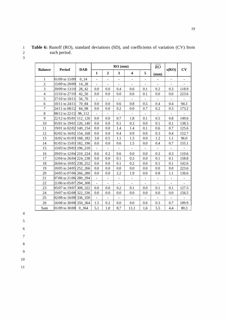
5. Runoff (RO) 25

The runoff was very small in relation to the other components (1.7% in relation to 26

rainfall) and presented a great variability, not appearing in all plots and in an unconsistant 27

way. This means that the coffee crop planted on a 10% slope along contour-lines was 28

adequate for runoff control and, consequently, erosion. 29

Insert Table 6 30

10

The high CVs presented in table 6 have to be analysed carefully. The presence of 1

many null values may indicate that this variable probably does not follow the normal 2

distribution and with very low mean values, CVs tend to increase by definition, even when 3

the variable is correctly measured. Anyway, the absolute values of RO were very small and 4

affected very little the establishment of water balances. 5

6 6. Water balances 7

Table 7 shows all water balance components in a joint way. 8

Insert Table 7 9

The historic average of annual rainfall in the city of Piracicaba is 1,275 mm, which 10

shows that this year (Sept.2003/Sept.2004) was slightly more rainy than normal. The 11

irrigation in this region is not necessary for the majority of the perennial crops, such as 12

coffee. The amount of irrigation water applied (71.6 mm) was only for preventing 13

blooming to be damaged during water stress periods. Considering water inputs (P+I), it is 14

verified that RO represents only 0.4% of the balance, which means that this component was 15

insignificant under the experimental conditions evaluated in this study. Figure 1 shows a 16

tendency of increasing RO as a function of increasing P. This fact is expected, but is very 17

hard to be forecasted once RO depends more on rain intensity than on the total amount of 18

water. It is also influenced by )( iL tS , which when low favours water infiltration. 19

The drainage below the depth z =1.0 m was 12.5% of the balance, which can be 20

more significant in wetter years. In terms of N leaching, a reflex of drainage, it can be 21

concluded that the coffee fertilization and its splitting were adequate in relation to the water 22

balance components. 23

As the annual variation of S∆ should theoretically, be small over long periods such 24

as a year (-5.5 mm in our case), the remaining of the water balance is ER, representing 25

82.5%. Under an ideal situation, in which RO and QL are null, ER would represent 100% of 26

(P+I), that is, ER = (P+I). Such condition almost happened over the studied year. 27

Insert Figure 1 28

Insert Figure 2 29

11

Figure 2 shows the distribution of rainfall and of evapotranspiration along the year 1

(Sept.2003/Sept.2004). In general, the rainfall was well distributed, except for the unsual 2

high rainfall rate during June and July (balances 20 to 24), which are generally drier months 3

in the region. This exception guaranteed a good development of the crop. The end of the 4

dry seasons, represented by balances 1 and 2; 25 and 26, demanded irrigation. The highest 5

rainfall occurred during the balances 11 and 13, and, as a consequence, the drainage (QL) 6

was 12.5% of (P+I). 7

The actual evapotranspiration got closer to the maximum almost along the whole 8

year, except for the dry periods (balances 1, 2, 4, 23, 25, and 26). During these periods, the 9

coffee plants lost part of their leaves because the soil hydraulic conductivity was too low, 10

defining a water flux to the plant root system that does not attend the atmospheric demand. 11

12

CONCLUDING REMARKS 13

1) Rainfall is generally measured only at one point and, in many cases one takes the 14

value of the nearest meteorological station. We verified that in experimental areas 15

having obstacles nearby which affect the dynamics of the wind and, consequently, 16

of the rainfall, the measurement of the rainfall should be made with an adequate 17

number of replicates. In our case, an area of 0.2 ha, with trees, silo, and 18

warehouse located within 100 m of distance, 5 rain-gauges apart from each other 19

by 15 to 100 m, presented CVs up to 17.8%; 20

2) Irrigation can introduce great variability in water balance calculations when not 21

well controlled, due to operational problems and wind drift; 22

3) The atmospheric demand of the coffee crop, expressed by its actual 23

evapotranspiration, was 1141.7 mm per year. It was not affected by the 24

parameters that characterize the stadia of growth and development of the crop. Its 25

estimation through water balance calculations is not recommended due to error 26

propagation. Alternative aerodynamic methods are better choices; 27

12

4) The soil in question presents a maximum capacity of soil water storage of the 1

order of 125 mm, which represents a backup of water for 25 days, without 2

considering the restrictions on water flux to the roots in drier periods and 3

considering an average demand of 5 mm/day. In this year the rainfall was near to 4

the long term average, and was enough to meet the atmospheric demand of the 5

crop, with restrictions in the period of dry and cold winter, favorable for 6

blossoming. Soils with smaller storage capacity are likely to cause water supply 7

problems and also permit larger values of internal drainage and, consequently, 8

leaching. Soil water storage, although measured carefully, was the component that 9

introduced most variability and error propagation in water balances; 10

5) The planting of coffee in areas with slopes has to be made in such a way to 11

provide good water infiltration, minimizing runoff losses and the erosion process. 12

Planting made in furrows along contour-lines, reduced considerably the runoff and 13

the erosion was nil. In our case, with an average slope of 10%, the value runoff 14

was very small, of the order from 1.7% in total of the rainfall. As expected, a 15

positive relation between the runoff and the rainfall was observed. 16

17

REFERENCES 18

19

GREMINGER, P.J.; SUD, Y.K.; NIELSEN, D.R. Spatial variability of field measured soil-20 water characteristics. Soil Science Society of America Journal, v. 40, p. 1075-1081, 21 1985. 22

23

IAFFE, A.; ARRUDA, F. B.; SAKAI, E. Simulação do consumo diário de água do cafeeiro 24 baseado em amostragens eventuais da umidade do solo em Pindorama, SP. In: Simpósio 25 de Pesquisas dos Cafés do Brasil, 1., 2000. Poços de Caldas, MG. Resumos 26 expandidos... Brasília; EMBRAPA Café e MINASPLAN, 2000. 786p. 27

28

LIBARDI, P.L.; SAAD, A.M. Balanço hídrico em cultura de feijão irrigada por pivô 29 central em Latossolo Roxo. Revista Brasileira de Ciência do Solo, v. 18, p. 529-532, 30 1994. 31

13

1

PEREIRA, A.R.; VILLA NOVA, N.A.; Sediyama, G.C. Evapo(transpi)ração. Piracicaba: 2 FEALQ, 1997. 183p. 3

4

REICHARDT, K., TIMM, L.C. Solo, planta e atmosfera: conceitos, processos e 5 aplicações. Barueri, SP: Manole, 2004. 478p. 6

7

REICHARDT, K.; ANGELOCCI, L.R.; BACCHI, O.O.S.; PILOTTO, J.E. Daily rainfall 8 variability at a local scale (1,000 ha), in Piracicaba, SP, Brazil, and its implications on 9 soil water recharge. Scientia Agricola, v. 52, p. 43-49, 1995. 10

11

TIMM, L. C. Efeito do manejo da palha da cana-de-açúcar nas propriedades físico-hídricas 12 de um solo. Piracicaba, SP, 2002. Tese (Doutorado em Agronomia) - Escola Superior de 13 Agricultura “Luiz de Queiroz”, Universidade de São Paulo. 14

15

VILLA NOVA, N. A. Dados agrometeorológicos do município de Piracicaba. 16 Piracicaba/Departamento de Física e Meteorologia, 1989. 17

18

VILLAGRA, M.M.; MATSUMOTO, O.M.; BACCHI, O.O.S.; MORAES, S.O.; 19 LIBARDI, P.L.; REICHARDT, K. Tensiometria e variabilidade espacial em terra roxa 20 estruturada. Revista Brasileira de Ciência do Solo, v. 12, p. 205-210, 1988. 21

22

VILLAGRA, M.M.; BACCHI, O.O.S.; TUON, R.L.; REICHARDT, K. Difficulties of 23 estimating evaporation from the water balance equation. Agricultural and Forest 24 Meteorology, v. 72, p. 317-325, 1995. 25

26 WARRICK, A.W.; NIELSEN, D.R. Spatial variability of soil physical properties in the 27

field. In: HILLEL, D. (Ed.). Applications of soil physics. New York: Academic Press, 28 1980. p. 319-344. 29

30 31 32 33 34 35 36 37 38 39 40 41 42 43

14

Table 1: Average rainfall (P), standard deviations [s(P)], and coefficients of variation (CV) 1 of each period. 2

3

Rainfall ( P ) Balance Period DAB 1 2 3 4 5 P s(P) CV

1 01/09 to 15/09 0_14 4.0 4.2 4.3 4.2 4.0 4.1 0.1 3.2 2 15/09 to 29/09 14_28 5.8 5.8 6.4 4.8 6.2 5.8 0.6 10.6 3 29/09 to 13/10 28_42 79.0 75.4 80.6 78.0 75.9 77.8 2.2 2.8 4 13/10 to 27/10 42_56 18.2 18.1 18.2 17.6 17.5 17.9 0.3 1.9 5 27/10 to 10/11 56_70 25.4 24.9 26.3 24.5 25.5 25.3 0.7 2.7 6 10/11 to 24/11 70_84 75.7 74.2 78.7 74.2 72.5 75.1 2.3 3.1 7 24/11 to 08/12 84_98 93.9 88.9 91.8 87.4 86.7 89.7 3.0 3.4 8 08/12 to 22/12 98_112 51.0 49.8 49.3 48.5 48.0 49.3 1.2 2.4 9 22/12 to 05/01 112_126 89.2 86.5 85.1 84.4 82.8 85.6 2.4 2.8 10 05/01 to 19/01 126_140 52.4 51.1 50.5 49.6 49.3 50.6 1.2 2.5 11 19/01 to 02/02 140_154 173.7 168.4 165.7 166.7 164.2 167.7 3.7 2.2 12 02/02 to 16/02 154_168 73.9 71.4 69.1 67.9 66.9 69.8 2.8 4.0 13 16/02 to 01/03 168_182 156.6 156.3 153.7 149.2 148.8 152.9 3.7 2.5 14 01/03 to 15/03 182_196 75.9 74.8 72.2 71.4 71.2 73.1 2.1 2.9 15 15/03 to 29/03 196_210 14.4 14.4 14.0 13.8 13.2 14.0 0.5 3.6 16 29/03 to 12/04 210_224 59.4 78.6 62.2 65.0 61.0 65.2 7.7 11.9 17 12/04 to 26/04 224_238 54.7 53.6 51.8 50.9 50.7 52.3 1.7 3.3 18 26/04 to 10/05 238_252 23.9 24.1 22.9 22.3 22.7 23.2 0.8 3.4 19 10/05 to 24/05 252_266 27.4 27.2 25.1 23.9 24.1 25.5 1.7 6.5 20 24/05 to 07/06 266_280 105.5 104.5 101.1 98.5 97.7 101.5 3.5 3.4 21 07/06 to 21/06 280_294 7.6 8.0 7.1 6.7 6.5 7.2 0.6 8.7 22 21/06 to 05/07 294_308 2.4 2.0 1.8 1.6 1.6 1.9 0.3 17.8 23 05/07 to 19/07 308_322 33.2 33.1 32.5 32.2 32.3 32.7 0.5 1.4 24 19/07 to 02/08 322_336 46.8 45.4 43.9 43.6 43.1 44.6 1.5 3.4 25 02/08 to 16/08 336_350 0.0 0.0 0.0 0.0 0.0 0.0 0.0 0.0 26 16/08 to 30/08 350_364 0.0 0.0 0.0 0.0 0.0 0.0 0.0 0.0

Sum 01/09 to 30/08 0-364 1350.0 1340.7 1314.3 1286.9 1272.4 1312.9 33.4 2.5 4 5 6 7 8 9 10 11 12 13 14 15 16

15

Table 2: Average irrigation )(I , standard deviations s(I), and coefficients of variation (CV) 1 for two periods. 2

3

Irrigation Balance Period DAB I s(I) CV

1 01/09 to 15/09 0_14 34.2 12.0 35.1 26 16/08 to 30/08 350_364 37.5 15.6 41.7

4 5

6

7

8

9

10

11

12

13

14

15

16

17

18

19

20

21

22

23

24

25

26

27

16

Table 3: Average actual evapotranspiration (ER’), its standard deviation [s(ER’) calculated 1 through equation 03], reference evapotranspiration (ET0), crop coefficient (KC), 2 potential evapotranspiration (ETC), ER and the drainage below root zone (QL) for 3 each period. 4

5

'ER 0ET CET ER=ER’-QL LQ Balance DAB

(mm) s(ER’) CV

(mm) KC

(mm) (mm) (mm)

1 0_14 -26.1 33,65 129,0 -45.9 1.1 -50.1 -26.1 0,0 2 14_28 -11.9 29,92 250,9 -56.0 1.1 -61.2 -11.9 0,0 3 28_42 -50.9 31,25 61,3 -53.9 1.1 -58.9 -50.9 0,0 4 42_56 -24.8 32,00 129,1 -65.4 1.1 -71.5 -24.8 0,0 5 56_70 -33.1 33,19 100,3 -47.5 0.7 -33.1 -33.1 0,0 6 70_84 -62.3 32,90 52,8 -60.3 1.0 -62.3 -62.3 0,0 7 84_98 -72.0 30,74 42,7 -50.5 1.4 -72.0 -72.0 0,0 8 98_112 -57.5 31,10 54,1 -62.4 0.9 -57.5 -57.5 0,0 9 112_126 -68.1 33,87 49,7 -57.5 1.2 -68.1 -68.1 0,0

10 126_140 -52.2 33,28 63,7 -63.2 0.8 -52.2 -52.2 0,0 11 140_154 -97.4 33,95 34,9 -39.3 1.1 -42.9 -42.9 -54,412 154_168 -95.5 34,66 36,3 -62.0 1.5 -95.5 -95.5 0,0 13 168_182 -130.6 35,80 27,4 -46.8 1.1 -51.2 -51.2 -79,414 182_196 -89.3 36,28 40,6 -52.3 1.7 -89.3 -89.3 0,0 15 196_210 -62.4 33,95 54,4 -55.3 1.1 -62.4 -62.4 0,0 16 210_224 -64.2 33,61 52,4 -47.7 1.3 -64.2 -64.2 0,0 17 224_238 -51.7 32,31 62,5 -36.1 1.4 -51.7 -51.7 0,0 18 238_252 -29.6 33,03 111,6 -35.6 0.8 -29.6 -29.6 0,0 19 252_266 -25.6 32,92 128,8 -24.4 1.0 -25.6 -25.6 0,0 20 266_280 -46.8 30,75 65,6 -23.4 1.1 -25.6 -25.6 -21,321 280_294 -19.6 31,51 160,5 -29.9 0.7 -19.6 -19.6 0,0 22 294_308 -21.9 33,59 153,2 -35.4 0.6 -21.9 -21.9 0,0 23 308_322 -6.6 31,13 469,1 -27.7 1.1 -30.2 -6.6 0,0 24 322_336 -57.5 30,00 52,2 -35.7 1.1 -39.0 -39.0 -18,525 336_350 -11.4 30,48 266,5 -45.1 1.1 -49.3 -11.4 0,0 26 350_364 -46.1 30,26 65,7 -46.7 1.1 -51.0 -46.1 0,0

1_26 0_364 -1315,3 - - -1206,0 1.1 -1318,3 -1141,7 -173,6 6

7

8

9

10

11

12

17

Table 4: Estimation of the standard deviation s(ER’) of the actual evapotranspiration ER’, 1 using error propagation (equation 03). 2

3

Balance DAB s(P) s(I) s(SF) s(SI) s(RO) s(ER')

1 0_14 0,1 12,0 20,7 23,7 0,0 33,6 2 14_28 0,6 0,0 21,6 20,7 0,0 29,9 3 28_42 2,2 0,0 22,5 21,6 0,3 31,2 4 42_56 0,3 0,0 22,8 22,5 0,0 32,0 5 56_70 0,7 0,0 24,1 22,8 0,0 33,2 6 70_84 2,3 0,0 22,3 24,1 0,4 32,9 7 84_98 3,0 0,0 21,0 22,3 0,3 30,7 8 98_112 1,2 0,0 22,9 21,0 0,0 31,1 9 112_126 2,4 0,0 24,8 22,9 0,8 33,9 10 126_140 1,2 0,0 22,1 24,8 0,1 33,3 11 140_154 3,7 0,0 25,5 22,1 0,7 33,9 12 154_168 2,8 0,0 23,3 25,5 0,4 34,7 13 168_182 3,7 0,0 26,9 23,3 1,1 35,8 14 182_196 2,1 0,0 24,3 26,9 0,7 36,3 15 196_210 0,5 0,0 23,7 24,3 0,0 34,0 16 210_224 7,7 0,0 22,5 23,7 0,3 33,6 17 224_238 1,7 0,0 23,1 22,5 0,1 32,3 18 238_252 0,8 0,0 23,6 23,1 0,1 33,0 19 252_266 1,7 0,0 22,9 23,6 0,0 32,9 20 266_280 3,5 0,0 20,2 22,9 1,1 30,7 21 280_294 0,6 0,0 24,2 20,2 0,0 31,5 22 294_308 0,3 0,0 23,3 24,2 0,0 33,6 23 308_322 0,5 0,0 20,6 23,3 0,1 31,1 24 322_336 1,5 0,0 21,7 20,6 0,0 30,0 25 336_350 0,0 0,0 21,4 21,7 0,0 30,5 26 350_364 0,0 15,6 14,7 21,4 0,7 30,3

4

5

6

7

8

9

10

11

12

13

18

Table 5: Soil water storage SL(ti), standard deviations s(SL), and coefficients of variation 1 (CV) of each period analyzed. 2

3

SI Balance Period DAB 1 2 3 4 5 LS s(SL) CV

1 01/09 to 15/09 0_14 250.2 260.8 203.4 254.6 257.2 245.2 23.7 9.7 2 15/09 to 29/09 14_28 261.0 271.1 221.0 265.6 268.3 257.4 20.7 8.0 3 29/09 to 13/10 28_42 255.9 265.6 213.1 259.3 262.4 251.3 21.6 8.6 4 13/10 to 27/10 42_56 272.3 284.5 242.8 303.0 286.9 277.9 22.5 8.1 5 27/10 to 10/11 56_70 269.9 280.3 232.8 292.2 279.9 271.0 22.8 8.4 6 10/11 to 24/11 70_84 263.2 276.0 221.5 278.7 276.8 263.3 24.1 9.2 7 24/11 to 08/12 84_98 273.0 287.4 238.7 296.3 282.5 275.6 22.3 8.1 8 08/12 to 22/12 98_112 286.3 306.7 262.3 317.2 293.1 293.1 21.0 7.2 9 22/12 to 05/01 112_126 277.9 299.8 249.8 309.2 288.0 284.9 22.9 8.0

10 05/01 to 19/01 126_140 288.3 312.9 271.4 336.9 299.9 301.9 24.8 8.2 11 19/01 to 02/02 140_154 288.0 311.4 270.2 328.0 303.2 300.2 22.1 7.4 12 02/02 to 16/02 154_168 380.0 380.2 324.5 384.3 380.6 369.9 25.5 6.9 13 16/02 to 01/03 168_182 352.1 354.8 302.6 359.5 350.8 344.0 23.3 6.8 14 01/03 to 15/03 182_196 375.4 382.3 317.4 375.2 375.3 365.1 26.9 7.4 15 15/03 to 29/03 196_210 356.2 364.1 305.4 359.2 357.7 348.5 24.3 7.0 16 29/03 to 12/04 210_224 310.5 314.4 258.0 311.5 306.0 300.1 23.7 7.9 17 12/04 to 26/04 224_238 304.5 317.2 261.9 315.4 305.2 300.8 22.5 7.5 18 26/04 to 10/05 238_252 305.0 313.3 261.0 318.2 309.2 301.3 23.1 7.7 19 10/05 to 24/05 252_266 301.0 306.4 253.0 308.7 305.4 294.9 23.6 8.0 20 24/05 to 07/06 266_280 300.2 304.8 254.3 306.1 308.8 294.8 22.9 7.8 21 07/06 to 21/06 280_294 360.1 359.9 312.8 356.2 354.3 348.7 20.2 5.8 22 21/06 to 05/07 294_308 348.4 348.7 293.3 342.0 348.7 336.2 24.2 7.2 23 05/07 to 19/07 308_322 327.7 327.7 274.8 321.6 329.2 316.2 23.3 7.4 24 19/07 to 02/08 322_336 350.7 345.4 306.0 353.7 355.3 342.2 20.6 6.0 25 02/08 to 16/08 336_350 341.4 334.6 290.7 337.9 341.7 329.3 21.7 6.6 26 16/08 to 30/08 350_364 334.1 324.3 280.4 322.9 327.4 317.8 21.4 6.7 4

5

6

7

8

9

10

11

12

19

Table 6: Runoff (RO), standard deviations (SD), and coefficients of variation (CV) from 1 each period. 2

3

RO (mm) RO Balance Period DAB

1 2 3 4 5 (mm) s(RO) CV

1 01/09 to 15/09 0_14 - - - - - - - - 2 15/09 to 29/09 14_28 - - - - - - - - 3 29/09 to 13/10 28_42 0.0 0.0 0.4 0.6 0.1 0.2 0.3 118.9 4 13/10 to 27/10 42_56 0.0 0.0 0.0 0.0 0.1 0.0 0.0 223.6 5 27/10 to 10/11 56_70 - - - - - - - - 6 10/11 to 24/11 70_84 0.0 0.0 0.6 0.8 0.5 0.4 0.4 94.3 7 24/11 to 08/12 84_98 0.0 0.0 0.2 0.0 0.7 0.2 0.3 173.2 8 08/12 to 22/12 98_112 - - - - - - - - 9 22/12 to 05/01 112_126 0.0 0.0 0.7 1.8 0.1 0.5 0.8 149.6

10 05/01 to 19/01 126_140 0.0 0.0 0.1 0.3 0.0 0.1 0.1 138.3 11 19/01 to 02/02 140_154 0.0 0.0 1.4 1.4 0.1 0.6 0.7 125.6 12 02/02 to 16/02 154_168 0.0 0.0 0.4 0.9 0.0 0.3 0.4 152.7 13 16/02 to 01/03 168_182 3.0 0.5 1.1 1.3 0.0 1.2 1.1 96.0 14 01/03 to 15/03 182_196 0.0 0.0 0.6 1.5 0.0 0.4 0.7 155.1 15 15/03 to 29/03 196_210 - - - - - - - - 16 29/03 to 12/04 210_224 0.6 0.2 0.6 0.0 0.0 0.3 0.3 110.6 17 12/04 to 26/04 224_238 0.0 0.0 0.1 0.3 0.0 0.1 0.1 158.8 18 26/04 to 10/05 238_252 0.0 0.0 0.1 0.2 0.0 0.1 0.1 142.6 19 10/05 to 24/05 252_266 0.0 0.0 0.0 0.0 0.0 0.0 0.0 223.6 20 24/05 to 07/06 266_280 0.0 0.0 2.2 1.9 0.0 0.8 1.1 136.6 21 07/06 to 21/06 280_294 - - - - - - - - 22 21/06 to 05/07 294_308 - - - - - - - - 23 05/07 to 19/07 308_322 0.0 0.0 0.2 0.1 0.0 0.1 0.1 127.3 24 19/07 to 02/08 322_336 0.0 0.0 0.0 0.0 0.0 0.0 0.0 156.5 25 02/08 to 16/08 336_350 - - - - - - - - 26 16/08 to 30/08 350_364 1.5 0.2 0.0 0.0 0.0 0.3 0.7 189.9

Sum 01/09 to 30/08 0_364 5,1 1,0 8,7 11,1 1,6 5,5 4,4 80,3 4

5

6

7

8

9

10

11

20

Table 7: Average values of rainfall ( P ), irrigation ( I ), soil water storage changes ( S∆ ), 1

runoff ( RO ), drainage ( LQ ), actual evapotranspiration ( ER ), and potential 2

evapotranspiration ( CET ), for all analyzed periods. 3

4

P I iS S∆ RO LQ ER CETBalance Period DAB (mm) (mm) (mm) (mm) (mm) (mm) (mm) (mm)

1 01/09 to 15/09 0_14 4.1 34.2 245.2 12.2 0.0 0.0 -26.1 -50.1 2 15/09 to 29/09 14_28 5.8 0.0 257.4 -6.1 0.0 0.0 -11.9 -61.2 3 29/09 to 13/10 28_42 77.8 0.0 251.3 26.6 -0.2 0.0 -50.9 -58.9 4 13/10 to 27/10 42_56 17.9 0.0 277.9 -6.9 0.0 0.0 -24.8 -71.5 5 27/10 to 10/11 56_70 25.3 0.0 271.0 -7.8 0.0 0.0 -33.1 -33.1 6 10/11 to 24/11 70_84 75.1 0.0 263.3 12.3 -0.4 0.0 -62.3 -62.3 7 24/11 to 08/12 84_98 89.7 0.0 275.6 17.5 -0.2 0.0 -72.0 -72.0 8 08/12 to 22/12 98_112 49.3 0.0 293.1 -8.2 0.0 0.0 -57.5 -57.5 9 22/12 to 05/01 112_126 85.6 0.0 284.9 17.0 -0.5 0.0 -68.1 -68.1 10 05/01 to 19/01 126_140 50.6 0.0 301.9 -1.7 -0.1 0.0 -52.2 -52.2 11 19/01 to 02/02 140_154 167.7 0.0 300.2 69.8 -0.6 -54.4 -42.9 -42.9 12 02/02 to 16/02 154_168 69.8 0.0 369.9 -26.0 -0.3 0.0 -95.5 -95.5 13 16/02 to 01/03 168_182 152.9 0.0 344.0 21.1 -1.2 -79.4 -51.2 -51.2 14 01/03 to 15/03 182_196 73.1 0.0 365.1 -16.6 -0.4 0.0 -89.3 -89.3 15 15/03 to 29/03 196_210 14.0 0.0 348.5 -48.4 0.0 0.0 -62.4 -62.4 16 29/03 to 12/04 210_224 65.2 0.0 300.1 0.7 -0.3 0.0 -64.2 -64.2 17 12/04 to 26/04 224_238 52.3 0.0 300.8 0.5 -0.1 0.0 -51.7 -51.7 18 26/04 to 10/05 238_252 23.2 0.0 301.3 -6.4 -0.1 0.0 -29.6 -29.6 19 10/05 to 24/05 252_266 25.5 0.0 294.9 -0.1 0.0 0.0 -25.6 -25.6 20 24/05 to 07/06 266_280 101.5 0.0 294.8 53.8 -0.8 -21.3 -25.6 -25.6 21 07/06 to 21/06 280_294 7.2 0.0 348.7 -12.4 0.0 0.0 -19.6 -19.6 22 21/06 to 05/07 294_308 1.9 0.0 336.2 -20.0 0.0 0.0 -21.9 -21.9 23 05/07 to 19/07 308_322 32.7 0.0 316.2 26.0 -0.1 0.0 -6.6 -30.2 24 19/07 to 02/08 322_336 44.6 0.0 342.2 -12.9 0.0 -18.5 -39.0 -39.0 25 02/08 to 16/08 336_350 0.0 0.0 329.3 -11.4 0.0 0.0 -11.4 -49.3 26 16/08 to 30/08 350_364 0.0 37.5 317.8 -8.9 -0.4 0.0 -46.1 -51.0

Sum 01/09 to 30/08 0_364 1312.8 71.6 7931.6 63.7 -5.5 -173.6 -1141.7 -1336.1 5

6

21

RO = 0.0054 P - 0.0588R2 = 0.6605

-0,2

0,0

0,2

0,4

0,6

0,8

1,0

1,2

1,4

0 20 40 60 80 100 120 140 160 180

P (mm)

RO (m

m)

1

Figure 1: Variations in the runoff, RO (mm), as a function of the rainfall, P (mm). 2

3 4

22

-110,0-100,0-90,0-80,0-70,0-60,0-50,0-40,0-30,0-20,0-10,0

0,010,020,030,040,050,060,070,080,090,0

100,0110,0120,0130,0140,0150,0160,0170,0180,0190,0

14 28 42 56 70 84 98 112 126 140 154 168 182 196 210 224 238 252 266 280 294 308 322 336 350 364

DAI

P, I,

ER

i, ET

c (m

m)

P I ERi ETc1

2 Figure 2: Variations in the rainfall (P), irrigation (I), actual evapotranspiration (ERi), and 3

potential evapotranspiration (ETc), in mm, 4