collective pairwise classification for multi-way...

COLLECTIVE PAIRWISE CLASSIFICATIONFOR MULTI-WAY ANALYSIS OF DISEASE AND DRUG DATA

MARINKA ZITNIK

Faculty of Computer and Information Science, University of Ljubljana,Vecna pot 113, SI-1000 Ljubljana, Slovenia

E-mail: [email protected]

BLAZ ZUPAN

Faculty of Computer and Information Science, University of Ljubljana,Vecna pot 113, SI-1000 Ljubljana, Slovenia, and

Department of Molecular and Human Genetics, Baylor College of Medicine,One Baylor Plaza, Houston, TX, 77030, USA

E-mail: [email protected]

Interactions between drugs, drug targets or diseases can be predicted on the basis of molecular, clinical and ge-nomic features by, for example, exploiting similarity of disease pathways, chemical structures, activities across celllines or clinical manifestations of diseases. A successful way to better understand complex interactions in biomed-ical systems is to employ collective relational learning approaches that can jointly model diverse relationshipspresent in multiplex data. We propose a novel collective pairwise classification approach for multi-way data analy-sis. Our model leverages the superiority of latent factor models and classifies relationships in a large relational datadomain using a pairwise ranking loss. In contrast to current approaches, our method estimates probabilities, suchthat probabilities for existing relationships are higher than for assumed-to-be-negative relationships. Although ourmethod bears correspondence with the maximization of non-differentiable area under the ROC curve, we were ableto design a learning algorithm that scales well on multi-relational data encoding interactions between thousands ofentities. We use the new method to infer relationships from multiplex drug data and to predict connections betweenclinical manifestations of diseases and their underlying molecular signatures. Our method achieves promising pre-dictive performance when compared to state-of-the-art alternative approaches and can make “category-jumping”predictions about diseases from genomic and clinical data generated far outside the molecular context.

Keywords: Collective classification, multi-relational learning, three-way model, drug-drug interactions,drug-target interactions, symptoms-disease network, gene-disease network

1. IntroductionCollective relational learning is concerned with data domains where entities like drugs, diseases andgenes are interconnected through multiple relations, such as drug-drug and drug-target interactions ordisease comorbidity.1–4 Since these approaches promote leaps across different data contexts, they areparticularly well suited to model large-scale heterogeneous collections of biomedical data and haveproven especially attractive for estimating binary relations, such as drug-drug interactions. These ap-proaches take advantage of the relational effects in the data by relying on relationships within one set ofentities when estimating relationships for the other entity set. For example, when predicting drug-targetinteractions relational approaches can consider the fact that drugs with similar pharmacological effectsare likely to interact with proteins with similar genomic sequences.1,2,5–7 Another example is mining ofdisease data, where relational approaches can benefit from observation that diseases caused by dysregu-lation of related pathways are likely to have similar clinical manifestation and show sensitivity to similarchemical compounds.3

State-of-the-art collective relational learning methods rely on latent factor modeling and typicallymeasure the fit of the models to the data through a regression metric, such as the root mean-squarederror, one-sided linear error or square penalty.3,8–12 The use of this metric in the search for best model

Pacific Symposium on Biocomputing 2016

81

parameters is especially appealing due to the well explored theory with many statistical guarantees aboutthe quality of least-squares solutions, efficient procedures for model estimation, and, in some cases, eventhe ability to find the optimal estimates. However, it is now widely recognized that approaches optimizingthe error rate, such as the root mean-squared error, can perform poorly with respect to ranking of therelationships.13,14 This situation gets exacerbated in practice where life scientists focus their attention ononly a small number of predicted relationships between entities, effectively ignoring all but a short list ofmost promising predicted relationships. For this reason, it is better to focus on correct prediction of smallbut highly likely set of relations than on accurately predicting all, even the irrelevant relationships.15

The predictive task we need to address is ranking where the aim is to rank the relationships accordingto their relevance. At first it may appear that learning a good regression model is sufficient for this task,as a model that achieves perfect regression will also give perfect ranking. However, a model with near-perfect regression performance may have arbitrarily poor ranking performance. The vice versa also holdstrue: a perfect ranking model may give very poor regression estimates.16 The development of predictionmodels that optimize for a ranking metric and can accommodate heterogeneous biomedical relations istherefore a crucial step towards accurate identification of the most promising relationships.

Taking insights from the research reviewed above, we propose a general statistical method that canestimate relationships between entities, e.g., drugs and diseases, from multi-way data, e.g., drug-druginteractions and shared human disease symptoms. Our proposed method uses pairwise classificationscheme to directly optimize a ranking metric. It estimates a latent data model, which serves to makepredictions about pairwise entity relationships. The contributions in this work are:

• We present a generic collective pairwise classification (COPACAR) model for multi-way data analy-sis.a We derive COPACAR model from the maximum posterior estimator for optimal collective pairwiseclassification on multi-relational data. We show the analogies between COPACAR and the maximiza-tion of area under the ROC curve.

• For minimizing the loss function of COPACAR, we propose a learning algorithm that is based onstochastic gradient descent with bootstrap sampling of training triplets. The in silico experimentalresults show that our algorithm has favorable convergence results w.r.t. the number of required al-gorithm iterations and the size of subsampled data. COPACAR can be easily parallelized, which canfurther increase its scalability.

• We show how to apply COPACAR to two challenges arising in personalized medicine. In studies onmulti-way disease and drug data we demonstrate that our method is capable of making category-jumping inferences,17 i.e. it can make predictions within and across informational contexts.

• Our experiments show that for the task of collective learning on multi-relational disease and drug data,learning a model with COPACAR outperforms approaches based on tensors and their decompositions.

Below we first overview related approaches for multi-relational learning and tensor decomposition.We then formulate a novel collective pairwise classification model and discuss the model fitting proce-dure. We present two case studies where we (1) investigate the connections between clinical manifesta-tions of diseases and their molecular interactions, and (2) study the interactions between drugs based ondrug-drug and drug-target relationships, structural similarities of the compounds, known pharmacologi-cal effects and interaction information extracted from the literature.

2. Related WorkCollective learning11 is an umbrella term for the mechanisms that exploit information, such as that onrelated classes, additional attributes or relationships between related entities, to support various learning

aThe online repository http://github.com/marinkaz/copacar includes the data and the source code used in this paper as well asadditional material for experiments in a non-biological domain.


82

tasks on multi-relational data, like classification, link prediction in networks and association mining. Theliterature on relational learning is vast, hence we only give a very brief overview.

Relational learning approaches18 assume that relations between entities arise from the interactionsbetween intrinsic latent attributes of these entities.10 Until recently, these approaches focused mostly onmodeling a single relation as opposed to trying to consider a collection of similar relations. However,recently made observations that relations can be highly similar or related3,10–12,19 suggested that super-imposing models learned independently for each relation would be ineffective, especially because therelationships observed for each relation can be extremely sparse. We here approach this challenge byproposing a collective learning approach that jointly models many data relations.

Probabilistic modeling approaches for relational (network) data often translate into learning an em-bedding of the entities into a low-dimensional manifold. Algebraically, this corresponds to a factorizationof an appropriately defined data matrix.3 A natural extension to modeling of many relations is to stackdata matrices and regard them as a tensor.10,11,20 Another extension to simultaneously learning many re-lations is to share a common embedding or the entities across different relations via collective matrixfactorization.9,21 An extensive review of tensor decompositions and other relational learning approachescan be found in Nickel et al.19

Several clustering-based approaches have been proposed for multi-relational learning. These includeclassical stochastic blockmodels, which associate a latent class to each entity in a domain; mixed member-ship stochastic blockmodels, which allow entities to have a mixed clusters membership;22 non-parametricBayesian models, which automatically infer the number of latent clusters;8,23 and neural network archi-tectures, which embed symbolic data representations into a flexible continuous vector space.24 Manynetwork modeling approaches25–27 try to detect local dependencies among the entities, i.e. nodes, andaccordingly group the nodes from a multiplex network into densely interconnected groups.

Unlike clustering-based approaches, COPACAR has classification capabilities, which come frommodel inference based on a pairwise ranking loss. Furthermore, COPACAR uses a factorized model toestimate interactions between entities, so that we can apply our approach to large data domains. Ourapproach also differs from the matrix factorization approach in terms of estimation method: while matrixfactorization models rely on likelihood training, we explicitly try to make the probability for existingrelationships to be larger than for assumed-to-be-negative relationships.

3. Relational Data ModelingWe consider relational data consisting of triplets where each triplet encodes a relationship between twoentities that we call the subject and the object. A triplet 〈Ei,R(k), Ej〉 indicates that relation R(k) holdsbetween subject Ei and object Ej . We represent a triplet as a matrix element X(k)

ij , where matrix X(k)

encodes relationR(k). We model dyadic multi-relational data as a three-way tensor where two modes areidentically formed by the concatenated entities and the third dimension corresponds to the relations.

Fig. 1 illustrates our modeling method. We assume the data is given as a collection of m partiallyobserved matrices each of size n×n, where n is the number of entities and m is the number of relationsb.A matrix element X(k)

ij = 1 denotes existence of a relationship 〈Ei,R(k), Ej〉. Otherwise, for non-existingrelationships, the associated matrix elements are set to zero. Unknown relationships can have a desig-nated value so that they are ignored during model estimation.

We refer to a triplet also as a relationship. A typical example, which we discuss in greater detail inthe following sections, is in pharmacogenomics, where a triplet 〈Ei,R(1), Ej〉 might correspond to theinteraction between drug i and drug j, and a triplet 〈Ei,R(2), Ej〉 might represent the association of drugi and drug j through a shared target protein. The goal is to learn a single model of all relations, which can

bNote that unlike established techniques in multi-relational modeling,11 our model does not need a homogeneous data domain.That is, entities of the first two modes can each be of different type, such as drugs, patients, diseases, etc.


83

1

0

Least-squares type objective:

This paper:

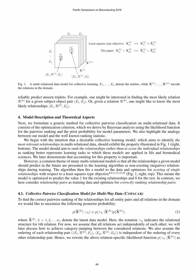
Fig. 1. A multi-relational data model for collective learning. E1, . . . , En denote the entities, while X(1), . . . ,X(m) encodethe relations in the domain.

reliably predict unseen triplets. For example, one might be interested in finding the most likely relationR(k) for a given subject-object pair (Ei, Ej). Or, given a relation R(k), one might like to know the mostlikely relationships 〈Ei,R(k), Ej〉.

4. Model Description and Theoretical AspectsNext, we formulate a generic method for collective pairwise classification on multi-relational data. Itconsists of the optimization criterion, which we derive by Bayesian analysis using the likelihood functionfor the pairwise ranking and the prior probability for model parameters. We also highlight the analogybetween our model and the well known ranking statistic.

We begin with the intuition that a desirable collective learning model, which aims to identify themost relevant relationships in multi-relational data, should exhibit the property illustrated in Fig. 1 (right,bottom). The model should aim to rank the relationships rather than to score the individual relationshipsas ranking better represents learning tasks to which these models are applied in life and biomedicalsciences. We later demonstrate that accounting for this property is important.

However, a common theme of many multi-relational models is that all the relationships a given modelshould predict in the future are presented to the learning algorithm as non-existing (negative) relation-ships during training. The algorithm then fits a model to the data and optimizes for scoring of singlerelationships with respect to a least-squares type objective8,9,11,21,23,28 (Fig. 1, right, top). This means themodel is optimized to predict the value 1 for the existing relationships and 0 for the rest. In contrast, wehere consider relationship pairs as training data and optimize for correctly ranking relationship pairs.

4.1. Collective Pairwise Classification Model for Multi-Way Data (COPACAR)To find the correct pairwise ranking of the relationships for all entity pairs and all relations in the domainwe would like to maximize the following posterior probability:

p(X(k)| >k) ∝ p(>k |X(k))p(X(k)), (1)

where X(k), k = 1, 2, . . .m, denote the latent data model. Here, the notation >k indicates the relationalstructure for kth relation. For now, we assume that all relations act independently of each other; we willlater discuss how to achieve category-jumping between the considered relations. We also assume theordering of each relationship pair (〈Ei,R(k), Ej〉, 〈Eg,R(k), Eh〉) is independent of the ordering of everyother relationship pair. Hence, we rewrite the above relation-specific likelihood function p(>k |X(k)) as


84

a product of single densities and then combine it for all relations k = 1, 2, . . . ,m as:∏k

p(>k |X(k)) =∏k

∏i,j,g,h

p(X(k)ij >k X

(k)gh )δ(X

(k)ij >kX

(k)gh )(1− p(X(k)

ij >k X(k)gh )δ(X

(k)ij 6>kX

(k)gh ), (2)

where δ is the indicator function, δ(x) is 1 if x is true and is 0 otherwise. Assuming that the properties ofa proper pairwise ranking scheme hold, we can further simplify the expression from Eq. (2) into:∏

k

p(>k |X(k)) =∏k

∏i,j,g,h

p(X(k)ij >k X

(k)gh )δ(X

(k)ij >kX

(k)gh ). (3)

So far it not guaranteed that the model produces a total ordering of the relationships in each rela-tion. To achieve this we need to satisfy the requirements for a total ordering. We do so by defining theprobability that relationship 〈Ei,R(k), Ej〉 is more relevant than relationship 〈Eg,R(k), Eh〉 as:

p(X(k)ij >k X

(k)gh ) , σ(X

(k)ij − X

(k)gh ), (4)

where σ(·) is the logistic function, σ(x) = 1/(1 + exp(−x)).Until now we delegated the task of modeling the relationship 〈Ei,R(k), Ej〉 to a yet unspecified latent

model X(k), k = 1, 2, . . .m,. We describe the model that can consider the intrinsic structure of multi-relational data. We build on the intuition from the RESCAL11,12 tensor decomposition and introduce thefollowing rank-r factorization, where each relation is factorized as:

X(k)ij = AT

i R(k)Aj , for k = 1, 2, . . . ,m. (5)

Here, A is a n× r matrix of latent components, where n represents the number of entities in the domainand r is dimensionality of the latent space. The rows of A, i.e., AT

i for i = 1, 2, . . . , n, model the latentcomponent representation of entities in the domain. Matrix R(k) is an asymmetric r × r matrix thatcontains the interactions of the latent components in kth relation.

When learning a large number of relations, i.e., when k is large, the number of observed relation-ships for each relation can be small, leading to a risk of overfitting. To decrease the overall number ofparameters, the model in Eq. (5) encodes relation-specific information with the latent matrices R(k) andembeds the entities into the latent space spanned by A. The effect of r � n is the automatic reuse oflatent parameters across relations. Collectivity of COPACAR is thus given by the structure of its model.

Thus far we discussed the likelihood function p(>k |X(k)). To determine the Bayesian approach fromEq. (1), we propose a prior p(X(k)), which is a normal distribution with a zero mean and a covariancematrix Σ:

p(A) ∼ N (0,ΣA), p(R(k)) ∼ N (0,ΣR), for k = 1, 2, . . . ,m. (6)

We further reduce the number of unknown parameters by setting ΣA = λAI and ΣR = λRI. We derive theoptimization criterion for our collective pairwise classification via the maximum posterior estimator:29

OPT-COPACAR , log p(X(k)| >k)= log p(>k |X(k))p(X(k))

= log∏k

p(>k |X(k))p(X(k))

= log∏k

∏i,j,g,h

σ(X(k)ij − X

(k)gh )δ(X

(k)ij >kX

(k)ij )p(X(k))

=∑k

∑i,j,g,h

`(X(k)ij − X

(k)gh ,X

(k)ij −X

(k)gh ) + λA‖A‖2 + λR

∑k

‖R(k)‖2Fro, (7)


85

where λA and λR are regularization parameters and pairwise classification loss function ` is formulatedas:

`(X(k)ij − X

(k)gh ,X

(k)ij −X

(k)gh ) = (X

(k)ij −X

(k)gh ) log σ(AT

i R(k)Aj −AT

gR(k)Ah). (8)

The COPACAR model rewards estimates of the model parameters that are in accordance with the inputdata. Intuitively, the semantics of the loss ` is as follows: (1) If X

(k)ij > X

(k)gh then 〈Ei,R(k), Ej〉 should

rank higher than 〈Eg,R(k), Eh〉, since it is assumed that the first relationship has greater relevance thanthe latter. Therefore, a model in which X

(k)ij > X

(k)gh holds, scores better on OPT-COPACAR than a model

with the two relationships ranked in the reversed order of their scores. (2) For relationships that are bothconsidered relevant, i.e. X(k)

ij = 1 and X(k)gh = 1, or both considered irrelevant, i.e. X(k)

ij = 0 and X(k)gh = 0,

we cannot infer any preference for their degree of relevance and the loss is unaffected by them.

4.2. Connection to the AUC OptimizationWe now show the analogy between OPT-COPACAR and area under the ROC curve (AUC). The AUCunder the ROC curve corresponds to the probability that a random existing (positive) relationship will bescored higher than a random non-existing (negative) relationship. The maximization of the AUC statisticis especially attractive in biomedical data domains, where the real objective is to optimize the sorting or-der, for example, to sort the relationships into a list so that relevant relationships are concentrated towardsthe top of the list.30 However, the problems with using the AUC statistic as an objective function are thatit is non-differentiable, and of complexity O(mn4) in the number of entities n, i.e., O(n2) relationshipsneed to be compared with themselves, and relations m in the domain. The AUC for relation k is usuallydefined across all pairwise comparisons of the relationships:

AUC(k) =1

N1(k)N0(k)

∑i,j

X(k)ij =1

∑g,h

X(k)gh =0

δ(X(k)ij − X

(k)gh > 0), (9)

where δ denotes the indicator function, andN1(k) andN0(k) count the existing (positive) and non-existing(negative) relationships in kth relation, respectively.

It is easy to see the analogy between the above formula and the maximum likelihood estimator inEq. (7). They differ in the normalization constant 1/(N1(k)N0(k)) and the definition of the loss func-tion. In contrast to the non-differentiable stepwise δ function used by the AUC, we employ the smoothloss log σ(x) in Eq. (8). Unlike many algorithms, which select a differentiable counterpart of a non-differentiable loss function in a heuristic manner,30 the COPACAR adopts the AUC statistic as its objectivefunction and specifies the loss function in Eq. (8) based on the maximum likelihood estimation.

4.3. Related Tensor FactorizationsThe factorization scheme specified in Eq. (5) builds on the RESCAL tensor decomposition11 and isrelated to other tensor decompositions. Specifically, it can be regarded as a generalization of the estab-lished DEDICOM, or an asymmetric extension of IDIOSCAL.11 The DEDICOM tensor model is givenas X(k) ≈ AD(k)RD(k)AT for k = 1, 2, . . . ,m. Here, the model assumes there is one global model ofinteractions between the latent components, i.e. an r × r latent matrix R. Notice that its variation acrossrelations is described by the r × r diagonal factors Dk. The diagonal matrices Dk contain membershipsof the latent components in the ktk relation. This is in contrast to Eq. (5) where we allow the relation-specific interactions for the latent components. While DEDICOM has been successfully applied to manydomains, for example to model the changes in the corporate communication and international trade overtime, our results suggest that its assumptions appear to be too stringent for multi-relational biologicaldata, which is aligned with the observations made by Nickel et al.11


86

Furthermore, the model in Eq. (5) is also different from traditional multi-way factor models, such asthe Tucker decomposition31 and CANDECOMP/PARAFAC (CP).32 The Tucker family defines a multi-linear form for a tensor X ∈ Rn×n×m as X = R ×1 A

(1) ×2 A(2) ×3 A

(3), where ×k denotes the mode-ktensor-matrix multiplication. Here, R is the global r1 × r2 × r3 tensor, and A(k) models the participa-tion of the latent components in the kth relation. The CP family is restricted form of the Tucker-baseddecompositions. The definition of rank-r CP for a tensor X ∈ Rn×n×m is given as a sum of componentrank-one tensors, al ∈ Rn, bl ∈ Rn and cl ∈ Rm, for l = 1, . . . , r. Elementwise, the CP decomposition iswritten as Xijk ≈

∑rl=1 ailbjlckl for i = 1, . . . , n, j = 1, . . . , n and k = 1, . . . ,m. The model in Eq. (5) can

be seen as a constrained variation of the CP model.11

One major difference of the COPACAR model in Eq. (7) to the existing tensor decompositions isthe objective criterion used for finding the latent matrices. Other tensor decompositions are restricted toleast-squares regression and cannot solve classification tasks, whereas COPACAR optimizes for a latentmodel with respect to ranking based on pairwise classification.

5. COPACAR Learning AlgorithmSo far we derived the optimization criterion for collective pairwise classification on multi-relational data.As the criterion in Eq. (7) is differentiable, gradient descent based algorithms are a natural choice for itsoptimization. However, standard gradient descent is not the most effective choice for our problem dueto the complexity of OPT-COPACAR (see Sec. 4.2). Instead, we propose a stochastic gradient descentalgorithm based on bootstrap sampling of training triplets.

Our aim is to find the latent matrices A and R(k) for k = 1, 2, . . . ,m that optimize for:

minA, R(k)

k=1,2,...,m

−OPT-COPACAR. (10)

The gradients of the pairwise loss from Eq. (8), the integral part of OPT-COPACAR, with respect to themodel parameters are:

∂

∂A`(X

(k)ij;gh,X

(k)ij;gh) = − ∂

∂AX

(k)ij;gh log σ(X

(k)ij;gh) = (σ(X

(k)ij;gh)− 1)X

(k)ij;gh

∂

∂AX

(k)ij;gh + λAA (11)

∂

∂R(k)`(X

(k)ij;gh,X

(k)ij;gh) = − ∂

∂R(k)X

(k)ij;gh log σ(X

(k)ij;gh) = (σ(X

(k)ij;gh)− 1)X

(k)ij;gh

∂

∂R(k)X

(k)ij;gh + λRR

(k),

where for simplicity of notation we write X(k)ij;gh = X

(k)ij − X

(k)gh .

Let Sk denote observed relationships in kth relation and let Ik represent non-edges in kth relation. Ifkth relation corresponds to the human disease symptoms network, then Sk contains all disease pairs withshared symptoms and Ik holds disease pairs for which shared disease symptoms have not been recorded.To achieve descent in a correct direction, the full gradient shall be computed over all training data in eachiteration and model parameters updated. However, since we have O(

∑k |Sk||Ik|) training triplets in the

data, computing the full gradient in each iteration is not feasible.Furthermore, optimizing OPT-COPACAR with a full gradient descent can lead to poor convergence

due to skewness of the training data. Consider for a moment a disease i with high symptom-based simi-larity to many other diseases. We have many terms for triplets of the form 〈Ei,R(symptom), Ej〉 in the lossbecause for many diseases j the disease i is compared against all diseases to which a particular diseasej is not related. Therefore, the gradients would be largely dominated by the terms depending on diseasei. This means that very small learning rates would need to be chosen and also regularization would bedifficult because the gradients would differ substantially.

To address the above issues we propose to use a stochastic gradient descent, which subsamples en-tity pairs (Ei, Ej) randomly (uniformly distributed) and forms an appropriately scaled gradient. In each


87

iteration we use a bootstrap sampling without replacement to pick entity combinations, and the Armijo-Goldstein step size control to determine the maximum amount to move along a given direction of descent.The chance of picking the same entity combination in consecutive update steps is hence small.

6. EvaluationNext, we test our algorithm for collective pairwise classification on two highly multi-relational datadomains. First, we apply it to the collection of relations between drugs, where we aim to predict differenttypes of drug relationships. We then study human disease data retrieved from the molecular and clinicalcontexts. We compare our method to tensor-based relational learning methods from Sec. 4.3.

6.1. A Case Study on Pharmacogenomic Data6.1.1. Data and Experimental Setup

We obtained a list of 1,451 drugs with known pharmacological actions from the DrugBank database.33

Examples of considered drugs include ospemifene, riluzole, chlormezanone and podofilox. Vast majorityof considered drugs contained links to the corresponding chemicals in the PubChem database,34 wherewe obtained information on similarity of their chemical structures. We also included information ondrug-target interactions33 and drug interaction data extracted from the literature through co-occurrencetext mining.35 Due to space constraints we refer to Kuhn et al.35 for a detailed description of relationshipsderived from text. We also mined the drug-drug interaction network, where we connected two drugs ifthey are known to interact, interfere or cause adverse reactions when taken together.33 The preprocesseddataset consisted of four drug-drug relations X(k) ∈ {0, 1}1451×1451 for k = 1, . . . , 4 and contained 59,990text associations, 2,602 interactions based on chemical structures, 1,315 interactions based on sharedtarget proteins and 48,614 drug-drug interactions based on adverse effects.

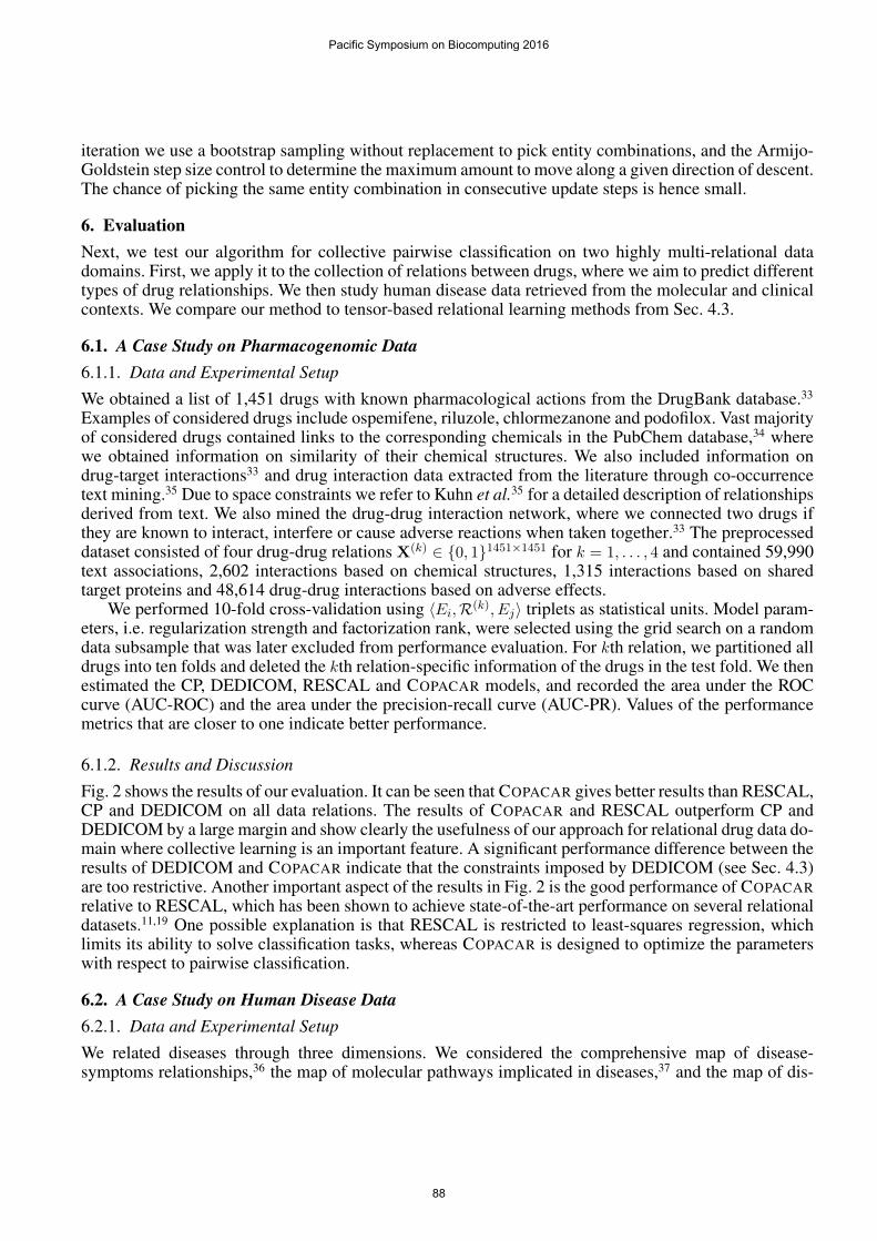
We performed 10-fold cross-validation using 〈Ei,R(k), Ej〉 triplets as statistical units. Model param-eters, i.e. regularization strength and factorization rank, were selected using the grid search on a randomdata subsample that was later excluded from performance evaluation. For kth relation, we partitioned alldrugs into ten folds and deleted the kth relation-specific information of the drugs in the test fold. We thenestimated the CP, DEDICOM, RESCAL and COPACAR models, and recorded the area under the ROCcurve (AUC-ROC) and the area under the precision-recall curve (AUC-PR). Values of the performancemetrics that are closer to one indicate better performance.

6.1.2. Results and Discussion

Fig. 2 shows the results of our evaluation. It can be seen that COPACAR gives better results than RESCAL,CP and DEDICOM on all data relations. The results of COPACAR and RESCAL outperform CP andDEDICOM by a large margin and show clearly the usefulness of our approach for relational drug data do-main where collective learning is an important feature. A significant performance difference between theresults of DEDICOM and COPACAR indicate that the constraints imposed by DEDICOM (see Sec. 4.3)are too restrictive. Another important aspect of the results in Fig. 2 is the good performance of COPACARrelative to RESCAL, which has been shown to achieve state-of-the-art performance on several relationaldatasets.11,19 One possible explanation is that RESCAL is restricted to least-squares regression, whichlimits its ability to solve classification tasks, whereas COPACAR is designed to optimize the parameterswith respect to pairwise classification.

6.2. A Case Study on Human Disease Data6.2.1. Data and Experimental Setup

We related diseases through three dimensions. We considered the comprehensive map of disease-symptoms relationships,36 the map of molecular pathways implicated in diseases,37 and the map of dis-


88

CP DEDICOM RESCAL COPACAR0.0

0.2

0.4

0.6

0.8

1.0

AU

C-R

OC

0.770 0.7420.880 0.900

Drug Associations from Text


0.2

0.4

0.6

0.8

1.0

AU

C-R

OC 0.669 0.718 0.798 0.863

Structural Similarity of Drugs


0.2

0.4

0.6

0.8

1.0

AU

C-R

OC

0.719 0.733 0.797 0.881Drug-Target Interactions


0.2

0.4

0.6

0.8

1.0

AU

C-R

OC 0.623

0.8000.909 0.924

Drug-Drug Interactions


0.2

0.4

0.6

0.8

1.0

AU

C-P

R

0.228 0.1730.268 0.318

Drug Associations from Text


0.2

0.4

0.6

0.8

1.0A

UC

-PR

0.144 0.177 0.203 0.225

Structural Similarity of Drugs


0.2

0.4

0.6

0.8

1.0

AU

C-P

R

0.229 0.258 0.283 0.333

Drug-Target Interactions


0.2

0.4

0.6

0.8

1.0

AU

C-P

R

0.253 0.276 0.3260.456

Drug-Drug Interactions

Fig. 2. The area under the ROC and the precision-recall (PR) curves via 10-fold cross-validation on drug data.

eases affected by various chemicals from the Comparative Toxicogenomics Database.37 We used therecent high-quality disease-symptoms data resource of Zhou et al.36 to generate a symptom-based rela-tion of 1,578 human diseases, where the link between two diseases indicated significant similarity of theirrespective symptoms. The details of the network construction based on large-scale medical bibliographicrecords and the related Medical Subject Headings (MeSH) metadata are described in Zhou et al.36 Ex-amples of considered diseases are Hodgkin disease, thrombocytosis, thrombocythemia and arthritis. Thepreprocessed dataset consisted of three disease-disease relations X(k) ∈ {0, 1}1578×1578 for k = 1, 2, 3 andcontained 117,021 relationships based on significant symptom similarity, 446,488 disease relationshipsderived from disease pathway information and 770,035 disease connections related to drug treatment.

In the evaluation we followed the experimental protocol described in Sec. 6.1.1.

6.2.2. Results and Discussion

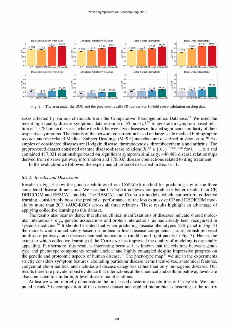
Results in Fig. 3 show the good capabilities of our COPACAR method for predicting any of the threeconsidered disease dimensions. We see that COPACAR achieves comparable or better results than CP,DEDICOM and RESCAL models. The RESCAL and COPACAR models, which can perform collectivelearning, considerably boost the predictive performance of the less expressive CP and DEDICOM mod-els by more than 20% (AUC-ROC) across all three relations. These results highlight an advantage ofapplying collective learning to this dataset.

The results also bear evidence that shared clinical manifestations of diseases indicate shared molec-ular interactions, e.g., genetic associations and protein interactions, as has already been recognized insystems medicine.36 It should be noted that when predicting disease phenotypes (left panel in Fig. 3)the models were trained solely based on molecular-level disease components, i.e. relationships basedon disease pathways and disease-chemical associations (middle and right panels in Fig. 3). Hence, theextent to which collective learning of the COPACAR has improved the quality of modeling is especiallyappealing. Furthermore, this result is interesting because it is known that the relations between geno-type and phenotype components remain unclear and highly entangled despite impressive progress onthe genetic and proteomic aspects of human disease.36 The phenotype map36 we use in the experimentsstrictly considers symptom features, excluding particular disease terms themselves, anatomical features,congenital abnormalities, and includes all disease categories rather than only monogenic diseases. Ourresults therefore provide robust evidence that interactions at the chemical and cellular pathway levels arealso connected to similar high-level disease manifestations.

At last we want to briefly demonstrate the link-based clustering capabilities of COPACAR. We com-puted a rank-30 decomposition of the disease dataset and applied hierarchical clustering to the matrix


89


0.2

0.4

0.6

0.8

1.0

AU

C-R

OC 0.654 0.704

0.824 0.848Human Disease Symptoms


0.2

0.4

0.6

0.8

1.0

AU

C-R

OC

0.775 0.830 0.911 0.933Disease Pathways


0.2

0.4

0.6

0.8

1.0

AU

C-R

OC

0.760 0.810 0.877 0.928Disease Chemicals


0.2

0.4

0.6

0.8

1.0

AU

C-P

R

0.244 0.234 0.2530.332

Human Disease Symptoms


0.2

0.4

0.6

0.8

1.0A

UC

-PR 0.665 0.678 0.748

0.840

Disease Pathways


0.2

0.4

0.6

0.8

1.0

AU

C-P

R

0.700 0.7220.881 0.924

Disease Chemicals

Fig. 3. The area under the ROC and the precision-recall (PR) curves via 10-fold cross-validation on disease data.

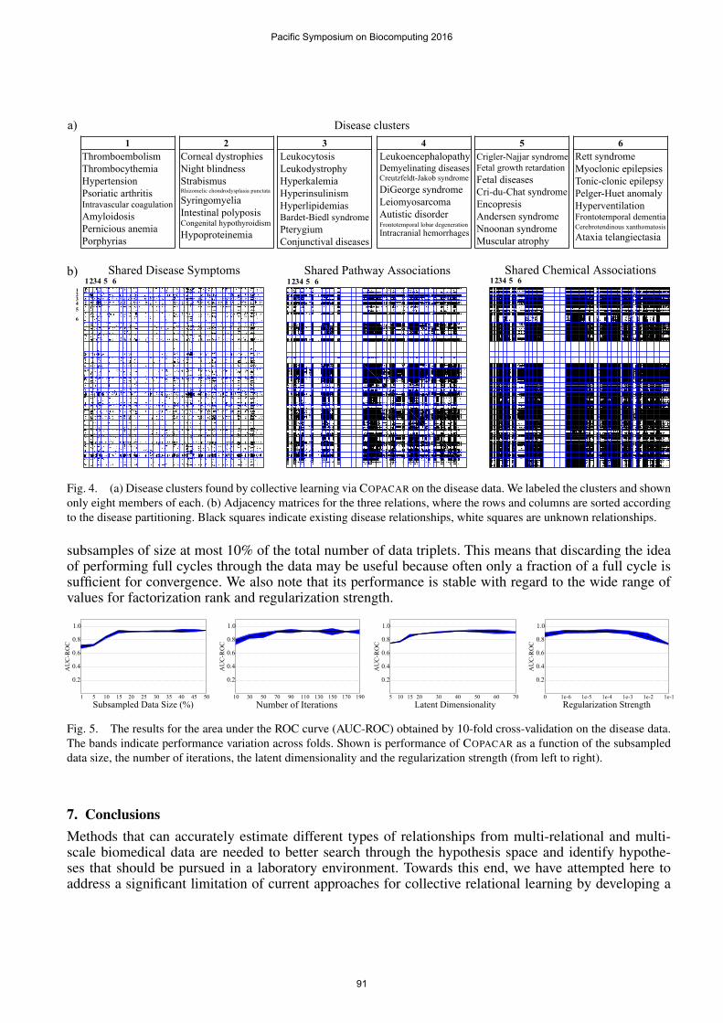
A (Fig. 4b). Diseases from the six randomly chosen clusters in Fig. 4a illustrate that we obtained ameaningful partitioning of the diseases and suggest that low-dimensional embedding of the data foundby COPACAR can be a useful resource for further data modeling. Here, we were especially interested inthe diseases grouped within the white bands in Fig. 4b (middle, right). Diseases therein have extremelysparse, if any at all, data profiles at the molecular or chemical levels. On the other hand, it can be seenfrom Fig. 4b (left) that these diseases have many common clinical phenotypes. Interestingly, COPACARwas able to make a leap across the three modeled disease dimensions and assigned poorly characterizeddiseases to clusters with richer molecular knowledge, such as phenylketonuria to the cluster centeredaround Parkinson’s disease. Even when not category-jumping, COPACAR grouped diseases, such as seb-orrheic dermatitis and herpes, based on their symptom similarity.

6.3. Runtime Performance and Technical ConsiderationsWe recorded the runtime of CP, DEDICOM, regularized RESCAL and COPACAR on various datasetsand for different factorization ranks (exact times are not shown due to the space limit). The COPACARshows training times below 3 minutes per fold on the disease data and below 5 minutes per fold on thedrug data. In comparison to CP and DEDICOM, it is the case that COPACAR as well as RESCAL oftengive a huge improvement in terms of runtime performance on real data.

In comparison to COPACAR, we observed that RESCAL can run up to three times faster on thesame data and using the same rank. We believe this is the case because RESCAL is optimized using thealternating least squares, which is possible due to its squared loss objective. In contrast, COPACAR is op-timized by a stochastic gradient descent due to the nature of its optimization criterion: in each iteration,it constructs a random data subsample and makes the update. The COPACAR algorithm has two impor-tant advantages over RESCAL. First, the algorithm naturally allows for parallelization of the gradientcomputation on a data subsample, which further increases scalability of COPACAR. Furthermore, we donot need to have collected the entire data relations to run the algorithm. Because COPACAR operates onsubsamples, it gives a natural approach for interleaving data collection and model estimation.

We also studied the technical aspects of the COPACAR learning algorithm. Specifically, we wereinterested in (1) the stability of algorithm performance w.r.t. the data subsample size, (2) its empiricalconvergence rate, and (3) its sensitivity to model parameters. Fig. 5 shows the results of this evaluation.In our experiments the algorithm typically required less than 100 iterations to converge and operated on


90

a)1

Disease clusters

ThromboembolismThrombocythemiaHypertensionPsoriatic arthritisIntravascular coagulationAmyloidosisPernicious anemiaPorphyrias

2Corneal dystrophiesNight blindnessStrabismusRhizomelic chondrodysplasia punctata

SyringomyeliaIntestinal polyposisCongenital hypothyroidismHypoproteinemia

3LeukoencephalopathyDemyelinating diseasesCreutzfeldt-Jakob syndromeDiGeorge syndromeLeiomyosarcoma Autistic disorderFrontotemporal lobar degenerationIntracranial hemorrhages

4LeukocytosisLeukodystrophyHyperkalemiaHyperinsulinismHyperlipidemiasBardet-Biedl syndromePterygiumConjunctival diseases

5Crigler-Najjar syndromeFetal growth retardationFetal diseasesCri-du-Chat syndromeEncopresisAndersen syndromeNnoonan syndromeMuscular atrophy

6Rett syndromeMyoclonic epilepsies Tonic-clonic epilepsy Pelger-Huet anomalyHyperventilationFrontotemporal dementiaCerebrotendinous xanthomatosisAtaxia telangiectasia

12345

6

b)2 4 5 61 3 2 4 5 61 3 2 4 5 61 3

Fig. 4. (a) Disease clusters found by collective learning via COPACAR on the disease data. We labeled the clusters and shownonly eight members of each. (b) Adjacency matrices for the three relations, where the rows and columns are sorted accordingto the disease partitioning. Black squares indicate existing disease relationships, white squares are unknown relationships.

subsamples of size at most 10% of the total number of data triplets. This means that discarding the ideaof performing full cycles through the data may be useful because often only a fraction of a full cycle issufficient for convergence. We also note that its performance is stable with regard to the wide range ofvalues for factorization rank and regularization strength.

Fig. 5. The results for the area under the ROC curve (AUC-ROC) obtained by 10-fold cross-validation on the disease data.The bands indicate performance variation across folds. Shown is performance of COPACAR as a function of the subsampleddata size, the number of iterations, the latent dimensionality and the regularization strength (from left to right).

7. ConclusionsMethods that can accurately estimate different types of relationships from multi-relational and multi-scale biomedical data are needed to better search through the hypothesis space and identify hypothe-ses that should be pursued in a laboratory environment. Towards this end, we have attempted here toaddress a significant limitation of current approaches for collective relational learning by developing a


91

method for collective classification that is designed to optimize for a pairwise ranking metric. Our methodachieves favorable performance in resolving which entity pairs (e.g., drugs) are most likely to be asso-ciated through a given type of relation (e.g., adverse effects or shared target proteins) by appropriatelyformulating a probabilistic model for pairwise classification of relationships.

Most likely, the most substantial advantage of our proposed approach is “category-jumping,” whichwe exemplify in a case study with several relations about diseases. Category-jumping has helped us tomake predictions about disease interactions at the molecular level that stem from clinical phenotype datacollected far outside the molecular contexts. The implications for utility of such inference are profound.Predictions that arise from category-jumping may reveal important relationships between biomedicalentities that are withheld from today-prevailing models that are trained on data of a single relation type.Acknowledgments

This work was supported by the ARRS (P2-0209, J2-5480) and the NIH (P01-HD39691).

References1. Y. Yamanishi, M. Kotera, M. Kanehisa and S. Goto, Bioinformatics 26, i246 (2010).2. X. Chen, M.-X. Liu and G.-Y. Yan, Molecular BioSystems 8, 1970 (2012).3. M. Zitnik, V. Janjic, C. Larminie, B. Zupan and N. Przulj, Scientific Reports 3 (2013).4. F. Cheng and Z. Zhao, Journal of the American Medical Informatics Association 21, e278 (2014).5. M. Campillos, M. Kuhn, A.-C. Gavin, L. J. Jensen and P. Bork, Science 321, 263 (2008).6. J. Huang, C. Niu, C. D. Green, L. Yang, H. Mei and J. Han, PLoS Computational Biology 9, p. e1002998 (2013).7. S. V. Iyer et al., Journal of the American Medical Informatics Association 21, 353 (2014).8. Z. Xu, V. Tresp, K. Yu and H.-P. Kriegel, Learning infinite hidden relational models, in UAI, 2006.9. A. P. Singh and G. J. Gordon, Relational learning via collective matrix factorization, in KDD, 2008.

10. R. Jenatton et al., A latent factor model for highly multi-relational data, in NIPS, 2012.11. M. Nickel, V. Tresp and H.-P. Kriegel, A three-way model for collective learning on multi-relational data, in ICML, 2011.12. M. Nickel et al., Reducing the rank in relational factorization models by including observable patterns, in NIPS, 2014.13. A. Gunawardana and G. Shani, Journal of Machine Learning Research 10, 2935 (2009).14. P. Cremonesi et al., Performance of recommender algorithms on top-n recommendation tasks, in RecSys, 2010.15. Y. Shi et al., GAPfm: Optimal top-n recommendations for graded relevance domains, in ICKM, 2013.16. D. Sculley, Combined regression and ranking, in KDD, 2010.17. E. Horvitz and D. Mulligan, Science 349, 253 (2015).18. S. Dzeroski, Relational data mining (Springer, 2010).19. M. Nickel, K. Murphy, V. Tresp and E. Gabrilovich, arXiv:1503.00759 (2015).20. B. W. Bader, R. Harshman, T. G. Kolda et al., Temporal analysis of semantic graphs using ASALSAN, in ICDM, 2007.21. M. Zitnik and B. Zupan, IEEE Transactions on Pattern Analysis and Machine Intelligence 37, 41 (2015).22. E. M. Airoldi, D. M. Blei, S. E. Fienberg and E. P. Xing, Mixed membership stochastic blockmodels, in NIPS, 2009.23. C. Kemp et al., Learning systems of concepts with an infinite relational model, in AAAI, 2006.24. A. Bordes, J. Weston, R. Collobert and Y. Bengio, Learning structured embeddings of knowledge bases, in AAAI, 2011.25. P. J. Mucha, T. Richardson, K. Macon, M. A. Porter and J.-P. Onnela, Science 328, 876 (2010).26. Y. Sun et al., PathSim: Meta path-based top-k similarity search in heterogeneous information networks, in VLDB, 2011.27. M. Zitnik and B. Zupan, Bioinformatics 31, 230 (2015).28. P. Hoff, Modeling homophily and stochastic equivalence in symmetric relational data, in NIPS, 2008.29. S. Rendle et al., BPR: Bayesian personalized ranking from implicit feedback, in UAI, 2009.30. A. Herschtal and B. Raskutti, Optimising area under the ROC curve using gradient descent, in ICML, 2004.31. L. R. Tucker, Psychometrika 31, 279 (1966).32. R. A. Harshman, UCLA Working Papers in Phonetics 16, 1 (1970).33. V. Law et al., Nucleic Acids Research 42, D1091 (2014).34. Y. Wang, J. Xiao, T. O. Suzek, J. Zhang, J. Wang and S. H. Bryant, Nucleic Acids Research 37, W623 (2009).35. M. Kuhn et al., Nucleic Acids Research 40, D876 (2012).36. X. Zhou, J. Menche, A.-L. Barabasi and A. Sharma, Nature Communications 5 (2014).37. A. P. Davis et al., Nucleic Acids Research 43, D914 (2015).


92

collective pairwise classification for multi-way...

Documents