collective matrix factorization of predictors ... · collective matrix factorization of predictors,...

Collective Matrix Factorization of Predictors,Neighborhood and Targets for Semi-Supervised

Classification

Lucas Drumond1, Lars Schmidt-Thieme1, Christoph Freudenthaler1, and ArtusKrohn-Grimberghe2

1 ISMLL - Information Systems and Machine Learning LabUniversity of Hildesheim, Germany

http://www.ismll.uni-hildesheim.de2 AIS-BI University of Paderborn, Germany

{ldrumond,schmidt-thieme,freudenthaler}@ismll.de, [email protected]

Abstract. Due to the small size of available labeled data for semi-supervised learning, approaches to this problem make strong assump-tions about the data, performing well only when such assumptions holdtrue. However, a lot of effort may have to be spent in understandingthe data so that the most suitable model can be applied. This processcan be as critical as gathering labeled data. One way to overcome thishindrance is to control the contribution of different assumptions to themodel, rendering it capable of performing reasonably in a wide range ofapplications. In this paper we propose a collective matrix factorizationmodel that simultaneously decomposes the predictor, neighborhood andtarget matrices (PNT-CMF) to achieve semi-supervised classification. Bycontrolling how strongly the model relies on different assumptions, PNT-CMF is able to perform well on a wider variety of datasets. Experimentson synthetic and real world datasets show that, while state-of-the-artmodels (TSVM and LapSVM) excel on datasets that match their char-acteristics and have a performance drop on the others, our approachoutperforms them being consistently competitive in different situations.

Keywords: Semi-supervised classification; factorization models

1 Introduction

In certain domains, the acquisition of labeled data might be a costly proccessmaking it difficult to exploit supervised learning models. In order to surmountthis, the field of semi-supervised learning [2] studies how to learn from bothlabeled and unlabeled data. Given the small amount of available labeled data,semi-supervised learning methods need to make strong assumptions about thedata distribution. The most prominent assumptions (briefly discussed in Section2) are the cluster and the manifold assumption.

2 L. Drumond, L. Schmidt-Thieme, C. Freudenthaler, A. Krohn-Grimberghe

It is usually the case that, if such assumptions do not hold, unlabeled datamay be seriously detrimental to the algorithms performance [3]. As a conse-quence, determining in advance good assumptions about the data and develop-ing or choosing models accordingly may be as critical as gathering labeled data.In chapter 21 from [2] an extensive benchmark evaluation of semi-supervisedlearning approaches on a variety of datasets is presented resulting in no overallwinner, i.e. no method is consistently competitive at all datasets, so that onehas to rely on background knowledge about the data. General models that canwork well on different kinds of data offer a means to circumvent this pitfall. Onepromising family of models that work in this direction are factorization models[10]. Such models are flexible enough to fit different kinds of data without over-fitting (given that they are properly regularized). However, to the best of ourknowledge, there is no systematic evaluation of the capabilities of factorizationmodels as semi-supervised classifiers.

In this work, we show how semi-supervised learning can be approached as afactorization problem. By factorizing the predictor matrix, one can exploit unla-beled data to learn meaningful latent features together with the decision bound-ary. This approach however is suboptimal if the data is not linearly separable.Thus, we enforce neighboring points in the original space to still be neighbors inthe learned latent space by factorizing also the adjacency matrix of the nearestneighbor graph. We call this model the Predictor/Neighborhood/Target Collec-tive Matrix Factorization (PNT-CMF). While the state-of-the-art approachesmay usually be very effective in some datasets, they perform poorly in others;we provide empirical evidence that PNT-CMF can profit from unlabeled data,making them competitive in settings where different model assumptions holdtrue. The main contributions of the paper are:

– We propose PNT-CMF, a novel model for semi-supervised learning thatcollectively factorizes the predictor, neighborhood and target relation.

– We devise a learning algorithm for PNT-CMF that is based on simultaneousstochastic gradient descent over all three relations.

– In experiments on both synthetic and real-world data sets we show thatour approach PNT-CMF outperforms existing state-of-the-art methods forsemi-supervised learning. Especially we show that while existing approacheswork well for datasets with matching characteristics (cluster-like datasets forTSVM and manifold-like datasets for LapSVM), our approach PNT-CMFconsistently performs competitive under varying characteristics.

2 Related Work

For a thorough survey of literature on semi-supervised learning in general, thereader is referred to [2] or [15]. In order to learn from just a few labeled datapoints, the models have to make strong assumptions about the data. One cancategorize semi-supervised classification methods according to such assumptions.Historically, the first semi-supervised algorithms were based on the idea that, if

Collective Factorization for Semi-Supervised Classification 3

two points belong to the same cluster, they have the same label. This is called thecluster assumption. If this assumption holds, it is reasonable to expect that theoptimal decision boundary should stay in a low density region. Methods whichfall into this category are the transductive SVMs [5] and the information regu-larization framework [11]. As pointed out by [15], this assumption does not holdtrue if, for instance, the data is generated by two highly overlapping gaussians.In this case, a generative model like the EM with mixture models [8] would beable to devise an appropriate classifier.

The second most relevant assumption is that data points lie on a low dimen-sional manifold [1]. One can think of the manifold assumption as the clusterassumption on the manifold. A successful approach implementing this assump-tion is the class of algorithms based on manifold regularization [1] [7], whichregularizes the model by forcing points with short geodesic distances to havesimilar values for the decision function. Since the geodesic distances are com-puted based on the laplacian of a graph representation of the data, these methodscan also be regarded as graph-based methods. This class of semi-supervised algo-rithms define a graph where the nodes are the data points and the edge weightsare the similarity between them and are regularized to force neighboring nodesto have similar labels. Graph based methods like the one based on GaussianFields and Harmonic functions [16] and global consistency method [14] rely onthe laplacian of the similarity graph to achieve this. These methods can be seenas special cases of the manifold regularization framework [1].

All of those methods have shown to be effective when their underlying as-sumptions hold true. However, when this is not the case, their performance mightactually be worsened by unlabeled data. The factorization models proposed hereare more flexible regarding the structure of the data since (i) they do not assmedecision function lies in a low density region, but map the features to a spacewhere they are easily separable instead and (ii) enforces neighboring points tohave the same label by co-factorizing the nearest neighbor matrix, which contri-bution to the model can be adjusted so that the model is robust to datasets wherethis information is not relevant. Multi-matrix factorization as predictive modelshave been investigated by [10]. Previous work on the semi-supervised learning offactorization models has either focused on different tasks or had different goalsfrom this work. While we are here focused on semi-supervised classification,previous work has focused on other tasks like clustering [12] and non-linear un-supervised dimensionality reduction [13]. A closer match is the work from Liu etal. [6] which approaches multi-label classification. Their method relies on ad-hocsimilarity measures for instances and class labels that should be chosen for eachkind of data. While their method only works for multi-label cases, the approachpresented here deals with binary classification.

3 Problem formulation

In a traditional supervised learning problem, data are represented by a predictorsmatrix X, where each row represents an instance predictor vector xi ∈ R|F|, F


being the set of predictors, and a target matrix Y , with each row yi containingthe values of the target variables for the instance i. Depending on the task, Ycan take various forms. Since throughout the paper we will consider the binaryclassification setting, we assume Y to be a one dimensional matrix (i.e. a vector)y ∈ {−1,+1}|I|, where I the set of instances.

Generally speaking, a learning model uses some training data DTrain :=(XTrain,yTrain) to learn a model that is able to predict the values in some testdata yTest given XTest, all unseen when learning.

In the semi-supervised learning scenario, there are two distinct sets of traininginstances: the first comes with their respective labels, i.e. XTrain

L and yTrainL ; the

second is composed of training instances for which their respective labels are notknown during training time, i.e. XTrain

U , thus the training data is composed byDTrain := (XTrain

L , XTrainU ,yTrain

L ).At this point learning problems can again be separated in two different set-

tings. In some situations, it is known during the learning time which instancesshould have their labels predicted. This is called transductive learning [4]. Inother situations however, the focus is on learning a general model able to makepredictions based on instances unknown during learning, which is called theinductive setting.

4 Factorization models for Semi-supervised Classification

4.1 Classification as a Multi-Matrix Factorization Task

Factorization models [10] decompose and represent a matrix as a product of twofactor matrices X ≈ f(V,H) where f : Rn×k × Rm×k → Rn×m is a functionrepresenting how two factors can be used to reconstruct the original matrixX ∈ Rn×m. One common choice for f is fX(V,H) := V H>.

In some cases, two or more matrices need to be factorized at the same time.[10] propose a loss function for decomposing an arbitrary number of matrices.Be M the set of matrices to be factorized and Θ the set of factor matrices tobe learned, each matrix M ∈ M is reconstructed by M ≈ fM (θM1 , θM2), whereθM1

, θM2∈ Θ. Thus the overall loss is

J(Θ) :=∑

M∈MαM lM (M,fM (θM1

, θM2)) +Reg(Θ) (1)

where lM is a loss function that measures the reconstruction error of matrix M ,0 ≤ αM ≤ 1 is a hyperparameter defining the relative importance of each lossfor the general objective function, and Reg is some regularization function.

In a classification problem the predictor matrix X and their respective tar-gets y are given. A factorization model approximates X as a function of twolatent factor matrices V,H, i.e. X ≈ fX(V,H) and y as a function of w ∈ R1×k

and V , i.e. y ≈ fy(V,w). This way each row vi of matrix V is a k-dimensionalrepresentation of the instance xi. The predicted targets are found in the approx-imating reconstruction of y, i.e. y ≈ Vw>. This task can be defined as finding


the factor matrices V , w and H that optimize a specific case of equation 1,namely:

J(V,w, H) := α lX(X, fX(V,H)) + (1− α)ly(y, fy(V,w)) +Reg(V,w, H) (2)

For the purposes of this work, the approximation functions will be the prod-uct of the factor matrices, i.e.:

X ≈ fX(V,H) = V H>

y ≈ fy(V,w) = Vw>

This model allows for different possible choices for lX and ly. Since it iscommon to represent instances of a classification problem as real valued featurevectors (and this is the case for the datasets used in our experiments), we usedthe squared loss as lX . For ly, a number of losses are suited for classificationproblems. We use the hinge loss here, since we are dealing with binary classifica-tion problems. In principle, any loss function can be used, so the one that bestfits the task at hand should be selected.

One drawback of using the hinge loss is that it is not smooth, meaning thatit is less easy to optimize. To circumvent this, we use the smooth hinge lossproposed by [9]:

h(y, y) :=

12 − yy if yy ≤ 0,12 (1− yy)2 if 0 < yy < 1,

0 if yy ≥ 1

(3)

4.2 Neighborhood Based Feature Extraction

The model presented so far is flexible enough for fitting a variety of datasets, butit still can not handle non-linear decision boundaries unless a very high numberof latent dimensions is used, which are difficult to estimate from few labeleddata. On the top of that, if the data follow the manifold assumption (i.e. datapoints lying next to each other on the manifold tend to have the same labels),the factorization model presented so far, will not be able to exploit this fact tolearn better decision boundaries. Because we use a linear reconstruction of y,if the data is not linearly separable in the learned latent space, the algorithmwill fail to find a good decision boundary. This problem can be circumvented byforcing that the nearest-neighborhood relationship is maintained on the latentspace. This works because the factorization of y forces the labeled points fromdifferent classes to be further apart from each other in the latent space. Forcingthat the neighborhood in the original space is preserved in the latent spacewill make the unlabeled points to be “dragged“ towards their nearest labeledneighbor, thus separating clusters or structures in the data, making it easier tofind a good decision boundary that is linear in the latent space.


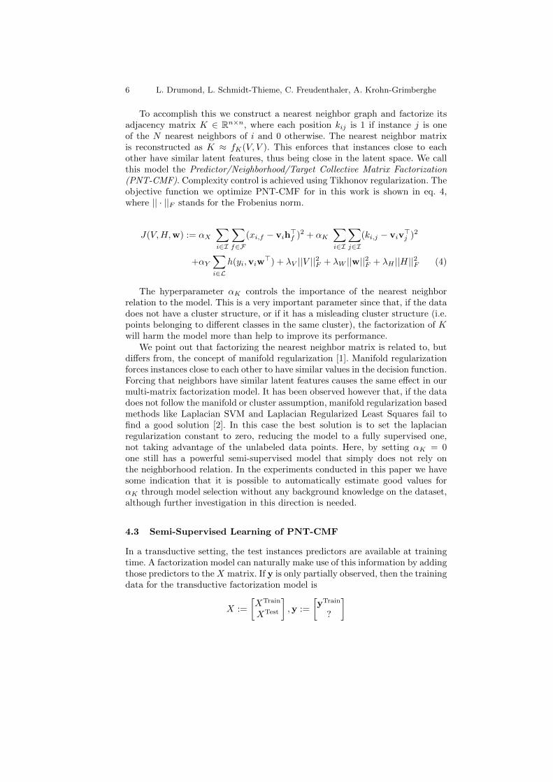
To accomplish this we construct a nearest neighbor graph and factorize itsadjacency matrix K ∈ Rn×n, where each position kij is 1 if instance j is oneof the N nearest neighbors of i and 0 otherwise. The nearest neighbor matrixis reconstructed as K ≈ fK(V, V ). This enforces that instances close to eachother have similar latent features, thus being close in the latent space. We callthis model the Predictor/Neighborhood/Target Collective Matrix Factorization(PNT-CMF). Complexity control is achieved using Tikhonov regularization. Theobjective function we optimize PNT-CMF for in this work is shown in eq. 4,where || · ||F stands for the Frobenius norm.

J(V,H,w) := αX

∑i∈I

∑f∈F

(xi,f − vih>f )2 + αK

∑i∈I

∑j∈I

(ki,j − viv>j )2

+αY

∑i∈L

h(yi,viw>) + λV ||V ||2F + λW ||w||2F + λH ||H||2F (4)

The hyperparameter αK controls the importance of the nearest neighborrelation to the model. This is a very important parameter since that, if the datadoes not have a cluster structure, or if it has a misleading cluster structure (i.e.points belonging to different classes in the same cluster), the factorization of Kwill harm the model more than help to improve its performance.

We point out that factorizing the nearest neighbor matrix is related to, butdiffers from, the concept of manifold regularization [1]. Manifold regularizationforces instances close to each other to have similar values in the decision function.Forcing that neighbors have similar latent features causes the same effect in ourmulti-matrix factorization model. It has been observed however that, if the datadoes not follow the manifold or cluster assumption, manifold regularization basedmethods like Laplacian SVM and Laplacian Regularized Least Squares fail tofind a good solution [2]. In this case the best solution is to set the laplacianregularization constant to zero, reducing the model to a fully supervised one,not taking advantage of the unlabeled data points. Here, by setting αK = 0one still has a powerful semi-supervised model that simply does not rely onthe neighborhood relation. In the experiments conducted in this paper we havesome indication that it is possible to automatically estimate good values forαK through model selection without any background knowledge on the dataset,although further investigation in this direction is needed.

4.3 Semi-Supervised Learning of PNT-CMF

In a transductive setting, the test instances predictors are available at trainingtime. A factorization model can naturally make use of this information by addingthose predictors to the X matrix. If y is only partially observed, then the trainingdata for the transductive factorization model is

X :=

[XTrain

XTest

],y :=

[yTrain

?

]


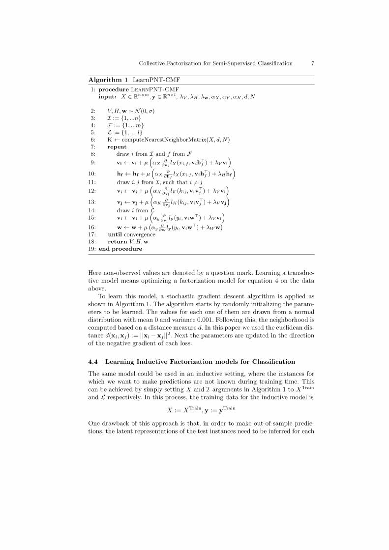
Algorithm 1 LearnPNT-CMF

1: procedure LearnPNT-CMFinput: X ∈ Rn×m,y ∈ Rn×l, λV , λH , λw, αX , αY , αK , d,N

2: V,H,w ∼ N (0, σ)3: I := {1, ...n}4: F := {1, ...m}5: L := {1, ..., l}6: K ← computeNearestNeighborMatrix(X, d,N)7: repeat8: draw i from I and f from F9: vi ← vi + µ

(αX

∂∂vi

lX(xi,f ,vih>f ) + λV vi

)10: hf ← hf + µ

(αX

∂∂hf

lX(xi,f ,vih>f ) + λHhf

)11: draw i, j from I, such that i 6= j

12: vi ← vi + µ(αK

∂∂vi

lK(kij ,viv>j ) + λV vi

)13: vj ← vj + µ

(αK

∂∂vj

lK(kij ,viv>j ) + λV vj

)14: draw i from L15: vi ← vi + µ

(αy

∂∂vi

ly(yi,viw>) + λV vi

)16: w← w + µ

(αy

∂∂wly(yi,viw

>) + λWw)

17: until convergence18: return V,H,w19: end procedure

Here non-observed values are denoted by a question mark. Learning a transduc-tive model means optimizing a factorization model for equation 4 on the dataabove.

To learn this model, a stochastic gradient descent algorithm is applied asshown in Algorithm 1. The algorithm starts by randomly initializing the param-eters to be learned. The values for each one of them are drawn from a normaldistribution with mean 0 and variance 0.001. Following this, the neighborhood iscomputed based on a distance measure d. In this paper we used the euclidean dis-tance d(xi,xj) := ||xi−xj ||2. Next the parameters are updated in the directionof the negative gradient of each loss.

4.4 Learning Inductive Factorization models for Classification

The same model could be used in an inductive setting, where the instances forwhich we want to make predictions are not known during training time. Thiscan be achieved by simply setting X and I arguments in Algorithm 1 to XTrain

and L respectively. In this process, the training data for the inductive model is

X := XTrain,y := yTrain

One drawback of this approach is that, in order to make out-of-sample predic-tions, the latent representations of the test instances need to be inferred for each


test instance separately. In other words, for a previously unseen instance xi, itsrespective latent feature vector vi is not computed during the training phase.We approach this problem by adding a fold-in step after learning the model.

The fold-in step takes a new instance xi and maps it to the same latentfeature space as the training instances. One straight-forward way to accomplishthis is to minimize Equation 5.

arg minvi

J(xi, H,vi) := αX ||xi − viH>||2 + αK ||ki − viV

>||2 + λV ||vi||2 (5)

5 Evaluation

The main goals of the experiments are: 1.) compare PNT-CMF against state-of-the-art semi-supervised classifiers; 2.) assess the robustness and competitivenessof our factorization model across datasets with different characteristics; 3.) ob-serve how useful semi-supervised transductive factorization models are comparedto their inductive supervised counterparts (i.e. we want to observe how much canfactorization models benefit from unlabeled data).

5.1 Datasets

Chapelle et al. [2] have run an extensive benchmark analysis of semi-supervisedlearning models on 6 datasets, which are also used here. The g241c, g241d,digit and usps datasets have all 1500 instances and 241 predictors while the bcidataset, 400 instances and 117 predictors. Finally the text dataset has 1500 in-stances and 11960 predictors. The task for all data sets is binary classification.Here we note that we conduct experiments only on binary classification in ordernot to contaminate the results with influences from different tasks. The applica-tion and evaluation of the model on other tasks like multi-class and multi-labelclassification and regression is left for future work.

5.2 Setup

For the evaluation of the methods proposed here, we employed the same protocolused in the benchmark analysis presented by [2]. Each dataset, comes with twodifferent sets of splits: the first one with 10 randomly chosen labeled traininginstances and the second with 100, each one with 12 splits. We used exactly thesame splits as [2], which are available for download3. Each model was evaluatedon a transductive semi-supervised setting. In order to be able to answer to ques-tion 3 posed in the beginning of this section, we also evaluated the models on afully supervised setting.

The performance of the model was measured using the hinge loss since itis the measure the evaluated models are optimized for. We also evaluated themodels on AUC but the results are suppressed here due to the lack of space. Thefindings from the experiments on both measures where however very similar.

3 http://olivier.chapelle.cc/ssl-book/benchmarks.html


5.3 Baselines

We compare PNT-CMF against representative methods implementing the twomost important assumptions of semi-supervised learning. As a representativeof the manifold assumption we chose the Laplacian SVM (LapSVM) trained inthe primal [7], since manifold regularization has been one of the most successfulapproaches for semi-supervised learning.

The second baseline is the transductive version of SVMs (TSVM) [5] whichimplements the low density (or cluster) assumption. On the inductive case,TSVM reduces to a standard SVM. Besides being representatives of their work-ing assumptions, both LapSVM and TSVM optimize the same loss used forPNT-CMF in this paper. Other graph based methods [16][14] work under thesame assumptions of LapSVM using a similar mathematical machinery (as dis-cussed in section 2) but optimize the squared loss instead. By having all thecompetitor methods optimizing the same loss, the effects observed come fromthe models only and not from the usage of different losses.

At last, since PNT-CMF performs dimensionality reduction and LapSVMoperates on a lower dimensional manifold, we add a fourth competitor methodwhich incorporates dimensionality reduction to TSVM as well: we applied PCAdimensionality reduction to all datasets and ran TSVM using the transformeddata. This method is called PCA+TSVM. For each dataset we used the first kPCA dimensions, k being the same number of latent dimensions used by PNT-CMF. As a TSVM implementation we used SVMLight4. For LapSVM we usedthe implementation from [7], which is also available for download5.

5.4 Model Selection and Reproducibility of the Experiments

Model selection is a known problem for semi-supervised learning due to the lownumber of labeled instances available. We show that it is possible to estimategood hyperparameters for PNT-CMF even in the presence of only a few labeleddata points. For PNT-CMF, each hyperparameter combination was evaluatedthrough 5-fold cross-validation using only the training data. The code forPNT-CMF can be made available upon request to the first author. We gavethe baseline methods a competitive advantage: use the same hyperparametersearch approach but employing both train and test data. We also observethat the results for the competitor methods are consistent with the ones reportedin the literature for the same datasets.

5.5 Results and discussion

The hinge loss scores for the datasets with 10 and 100 labeled examples are shownin Figure 1. For each method and dataset, the average performance over the 12splits is shown. The error bars represent the 99% confidence intervals. [2] divide

4 http://svmlight.joachims.org/5 http://www.dii.unisi.it/˜melacci/lapsvmp/


these datasets into two categories: the manifold-like and the cluster-like. Themanifold group comprises the digit, usps and bci datasets in which the data lienear a low dimensional manifold. Algorithms like LapSVM are expected to excelin these datasets. g241c, g241d and text fall under the category of cluster-likedatasets in which different classes do not share the same cluster thus makingthe optimal decision boundary to lie in a low density region, favoring algorithmslike TSVM.

Transductive semi-supervised

(a) 10 labeled instances

Inductive supervised

(b) 10 labeled instances

(c) 100 labeled instances (d) 100 labeled instances

Fig. 1: Results for the Hinge Loss. The lower the better.

The left-hand side of Figure 1 shows how PNT-CMF performs in comparisonto its competitors. By looking specially at this figure, one can see that TSVMis stronger in the g241c and text datasets while LapSVM is more competitivein the manifold-like data. One can also see that LapSVM is significantly weakeron the g241c and text sets where the data do not lie near a low dimensionalmanifold. PNT-CMF on the other hand is always either the statistically signifi-cant winner or is away from the winner by a non significant margin. Out of the12 experiments, PNT-CMF is the sole winner in 8 of them and is one of thewinning methods in all the 3 ties, with TSVM winning in one case, and onlyfor 100 labeled instances. We show here the Hinge loss results because this was


the measure all the models in the experiment are optimized for. As already saidwe also evaluated the AUC of these models in these experiments and the resultswere similar, with PNT CMF being the sole winner in 5 experiments and oneof the winning methods in the other 7. This supports our claim that PNT-CMFcan consistently work well under different assumptions. In accordance with ourexpectations, LapSVM is more competitive on the manifold-like datasets whileTSVM on the cluster-like ones.

Finally, by comparing the right and left hand sides of Figure 1, we can havean idea of the effects of taking unlabeled data into account. One can observethat TSVM seems to be more unstable, having sometimes worse hinge loss onthe semi-supervised case than the corresponding ones on the supervised scenariosfor the bci, usps and g241d datasets. The same happens for LapSVM on g241ddataset. PNT-CMF seems to be more robust in this sense, not presenting asignificant performance degradation in any case.

6 Conclusion

In this work we proposed PNT-CMF, a factorization model for semi-supervisedclassification and showed how to learn such models in a transductive (semi-supervised) and in an inductive (supervised) setting. The performance of suchmodels was evaluated on a number of different synthetic and real-world datasetswith varying characteristics. The proposed model relies on the reconstruction ofthe predictors and the neighborhood matrices in the original feature space tolearn latent factors used for classification. The contribution of each of them tothe model can be controlled in order to fit different kinds of datasets better.

PNT-CMF represents a step forward in the state-of-the-art because, unlikeother semi-supervised methods which face a performance degradation when theirmodel assumptions do not hold, the experimental results showed that PNT-CMFis capable of coping with datasets with different characteristics. One evidence forthis is that, in all cases, regardless of whether LapSVM or TSVM were the bestmodels, PNT-CMF was always a strong competitor, being among the winnersin the vast majority of the semi-supervised experiments.

As future work we plan to investigate better factorization strategies for thematrix K, like different loss and reconstruction functions. Also the extension andevaluation of the model on regression, multi-class and multi-label classificationtasks is an issue to be further investigated.

Acknowledgments. The authors gratefully acknowledge the co-funding oftheir work by the Multi-relational Factorization Models project granted by theDeutsche Forschungsgesellschaft6. Lucas Drumond is sponsored by a scholarshipfrom CNPq, a Brazilian government institution for scientific development.

6 http://www.ismll.uni-hildesheim.de/projekte/dfg_multirel_en.html


References

1. Belkin, M., Niyogi, P., Sindhwani, V.: Manifold regularization: A geometric frame-work for learning from labeled and unlabeled examples. The Journal of MachineLearning Research 7, 2399–2434 (2006)

2. Chapelle, O., Scholkopf, B., Zien, A. (eds.): Semi-Supervised Learning. MIT Press,Cambridge, MA (2006)

3. Cozman, F., Cohen, I., Cirelo, M.: Semi-supervised learning of mixture models. In:20th International Conference on Machine Learning. vol. 20, pp. 99–106 (2003)

4. Gammerman, A., Vovk, V., Vapnik, V.: Learning by Transduction. In: In Pro-ceedings of the Fourteenth Conference on Uncertainty in Artificial Intelligence. pp.148–156. Morgan Kaufmann (1998)

5. Joachims, T.: Transductive Inference for Text Classification using Support Vec-tor Machines. In: Proceedings of the 1999 International Conference on MachineLearning (ICML) (1999)

6. Liu, Y., Jin, R., Yang, L.: Semi-supervised multi-label learning by constrainednon-negative matrix factorization. In: Proceedings of the National Conference onArtificial Intelligence. vol. 21, p. 421. AAAI Press (2006)

7. Melacci, S., Belkin, M.: Laplacian Support Vector Machines Trained in the Primal.Journal of Machine Learning Research 12, 1149–1184 (March 2011)

8. Nigam, K., McCallum, A., Mitchell, T.: Semi-supervised text classification usingEM. In: Chapelle, O., Scholkopf, B., Zien, A. (eds.) Semi-Supervised Learning, pp.33–56. The MIT Press, Cambridge, MA (2006)

9. Rennie, J.: Smooth Hinge Classification (Feb 2005), http://people.csail.mit.edu/jrennie/writing/smoothHinge.pdf

10. Singh, A.P., Gordon, G.J.: Relational learning via collective matrix factorization.In: Proceeding of the 14th ACM SIGKDD International Conference on KnowledgeDiscovery and Data Mining. pp. 650–658. ACM, New York, NY, USA (2008)

11. Szummer, M., Jaakkola, T.: Information regularization with partially labeled data.Advances in Neural Information Processing Systems 15, 1025–1032 (2002)

12. Wang, F., Li, T., Zhang, C.: Semi-supervised clustering via matrix factorization.In: Proceedings of the 2008 SIAM International Conference on Data Mining. pp.1–12. SIAM (2008)

13. Weinberger, K., Packer, B., Saul, L.: Nonlinear dimensionality reduction bysemidefinite programming and kernel matrix factorization. In: Proceedings of theTenth International Workshop on Artificial Intelligence and Statistics. pp. 381–388(2005)

14. Zhou, D., Bousquet, O., Lal, T.N., Weston, J., Scholkopf, B.: Learning with localand global consistency. Advances in Neural Information Processing Systems 16,321–328 (2004)

15. Zhu, X.: Semi-supervised learning literature survey. Tech. Rep. 1530, University ofWisconsin, Madison (Dec 2006)

16. Zhu, X., Ghahramani, Z., Lafferty, J.: Semi-Supervised Learning Using GaussianFields and Harmonic Functions. In: Proceedings of the Twentieth InternationalConference on Machine Learning (ICML). pp. 912–919 (2003)

collective matrix factorization of predictors ... · collective matrix factorization of predictors,...

Documents