collapse vulnerability of reinforced concrete buildings
TRANSCRIPT

Collapse Vulnerability of Reinforced Concrete
Buildings Using Neural Networks
Imad Mohammad Alshaer
Submitted to the
Department of Civil Engineering
In partial fulfillment of the requirements for the degree of
Master of Science
in
Civil Engineering
Eastern Mediterranean University
September 2016
Gazimağusa, North Cyprus

Approval of the Institute of Graduate Studies and Research
_____________________
Prof. Dr. Mustafa Tümer
Acting Director
I certify that this thesis satisfies the requirements as a thesis for the degree of Masters
of Science in Civil Engineering.
________________________________
Assoc. Prof. Dr. Serhan Şensoy
Chair, Department of Civil Engineering
We certify that we have read this thesis and that in our opinion it is fully adequate in
scope and quality as a thesis for the degree of Master of Science in Civil
Engineering.
___________________________
Asst. Prof. Dr. Giray Özay
Supervisor
Examining Committee
1. Assoc. Prof. Dr. Mustafa Ergil ____________________________
2. Asst. Prof. Dr. Giray Özay ____________________________
3. Asst. Prof. Dr. Eriş Uygar ____________________________

iii
ABSTRACT
In this study, an Artificial Neural Network (ANN) analytical method has been
developed for evaluation the collapse vulnerability (earthquake performance) of
reinforced concrete (RC) buildings . In this study, collected total of 260 reinforced
concrete buildings with 4 storey, that were chosen to represent the existing RC
buildings. The commercial program Sta4CAD is used for modeling and analysing
these buildings. The performance analysis of these 260 RC buildings have been used
for training neural networks. The parameters that affect on earthquake performance
represent the input and the performance represent the output.
In this study 16 parameters have been thought to be effective on the performance of
RC buildings were considered: Torsional Irregularity (A1), Slab Discontinuities
(A2), Projections in Plan (A3), Weak Storey (B1), Soft Story (B2), Discontinuity of
Vertical Structural Elements (B3), Weak Column – Strong Beam (C2), Stirrup
Spacing (cm), Average Shear Wall Ratio, Average Column Ratio (CA) , Concrete
Compression Strength (C), Type of Steel (Fy), Soil Type (Z), Turkish Earthquake
Code (1975– 1997- 2007), Earthquake Zone (EZ) and Importance Factor (I). The
output parameters are the Structural Performance (S1-S4) was obtained based on the
4 performance levels in Turkish Earthquake Code-2007 (TEC-2007). The
performance analysis of RC buildings was performed according to both the linear
performance analysis and nonlinear (static pushover analysis) procedures as specified
in TEC-2007.

iv
The effect of each parameter tested in this study had various affecting ratios on the
earthquake performance of the structure. It was found that shear wall ratio is the most
significant structural components that affect. The projections in plan and slab
discontinuities were determined to be the least significant parameters. According to
the study, the prediction accuracy of ANN has been found 90% accuracy for
nonlinear (pushover analysis method) and about 89% accuracy for linear
performance analysis method.
Keywords: Artificial neural network, collapse vulnerability, earthquake performance
based design.
v
ÖZ
Bu çalışmada betonarme binaların deprem performanslarının değerlendirilmesi için
yapay sinir ağları kullanılmıştır. Bu maksatla 4 katlı 260 betonarme bina seçilmiştir.
Bu binalar Sta4CAD programı ile tasarlanmıştır. Binaların doğrusal elastik ve statik
itme performans analiz sonuçları kullanılarak, yapay sinir ağı eğitilmiştir.
Oluşturulan yapay sinir ağı sisteminde deprem performansını etkileyen parametreler
girişi, yapı performans seviyesi ise çıkışı temsil etmektedir.
Bu çalışmada deprem performansını etkileyeceği düşünülen 16 parametre seçilmiştir.
Bunlar: Burulma Düzensizliği (A1), Döşeme Süreksizliği (A2), Planda Çıkıntılar
Bulunması (A3), Zayıf Kat (B1), Yumuşak Kat (B2), Taşıyıcı Sistem Düşey
Elemanlarının Süreksizliği (B3), Güçlü Kolon-Zayıf Kiriş (C2), Etriye Aralığı (cm),
Ortalama Perde Duvar Oranı, Ortalama Kolon Oranı (CA), Beton Basınç Dayanımı
(C), Çelik Türü (Fy), Zemin Türü (Z), Türk Deprem Yönetmeliği (1975 – 1997 –
2007), Deprem Bölgesi (EZ) ve Bina Önem Katsayısı (I)'dır. Çıkış parametreleri ise
2007 Türk Deprem Şartnamasi’nde (TEC-2007) bulunan 4 bina performans
seviyesidir (S1-S4). Performans analizleri deprem şartnamesinde mevcut olan
doğrusal elastik ve statik itme performans analiz yöntemlerine göre yapılmıştır.
Bu çalışmada seçilen giriş parametreleri test edilmiş ve Ortalama Perde Duvar
Oranının deprem performasında en önemli parametre olduğu saptanmıştır. Planda
Çıkıntılar Bulunması ve Döşeme Süreksizliği parametreleri ise en az etkili
parametreler olarak saptanmıştır. Bu çalışmanın sonucunda oluşturulan yapay sinir
ağı sisteminde statik itme analizi yöntemi ile yapılan performans seviyesi

vi
tahminlerinin doğruluk oranının % 90, lineer performans analiz yöntemine göre
yapılan performans seviyesi tahminlerinin doğruluk oranının ise % 89 olduğu
saptanmıştır.
Anahtar Kelimeler: Yapay sinir ağları, göçme riski, deprem performansına dayalı
tasarım.

vii
DEDICATION
I dedicate this thesis to my family whom they supported me throughout my study.

viii
ACKNOWLEDGMENT
First of all, I would like to thank Allah for giving me this chance to get master
degree. Secondly, I would like to thank my supervisor Asst. Prof. Dr. Giray Özay for
his continuous support and guidance in the preparation of this study. Without his
invaluable supervision, all my efforts could have been short-sighted.
I owe quite a lot to my family who supported me all throughout my studies. I would
like to dedicate this study to them as an indication of their significance in this study
as well as in my life.

ix
TABLE OF CONTENTS
ABSTRACT ........................................................................................................... iii
ÖZ ............................................................................................................................v
DEDICATION....................................................................................................... vii
ACKNOWLEDGMENT ....................................................................................... viii
LIST OF TABLES ................................................................................................. xii
LIST OF FIGURES ...............................................................................................xiv
LIST OF ABBREVIATIONS .............................................................................. xvii
LIST OF SYMBOLS .......................................................................................... xviii
1 INTRODUCTION .................................................................................................1
1.1 General ..........................................................................................................1
1.2 Previous Studies on Rapid Assessment Methods for Seismic Vulnerability of
Existing Reinforced Concrete Buildings ..............................................................2
1.3 Previous Studies on Seismic Vulnerability Assessment using ANNs ..............4
1.4 General Objective ..........................................................................................6
1.5 Specific Objectives ........................................................................................6
1.6 Scope of Study...............................................................................................6
1.7 Research Methodology ..................................................................................7
1.8 Structure of the Thesis ...................................................................................7
2 GENERAL PRINCIPLES AND RULES OF EARTHQUAKE DESIGN ...............9
2.1. Introduction ..................................................................................................9
2.2. Earthquake Analysis According to TEC 2007 ..............................................9
2.3. Performance Analysis According to TEC-2007 ........................................... 18
3 ARTIFICIAL NEURAL NETWORKS ................................................................ 34

x
3.1 Introduction ................................................................................................. 34
3.2 Definition of Artificial Neural Networks ...................................................... 34
3.3 Terminology used in Artificial Neural Network ........................................... 35
3.4 Advantages and Disadvantages of ANN ...................................................... 36
3.5 Mechanism of Artificial Neural Networks.................................................... 38
3.6 Types of Artificial Neural Networks ............................................................ 39
3.7 Functions used in developing ANN.............................................................. 41
3.8 Algorithms used for Training Artificial Neural Network .............................. 42
4 METHODOLOGY .............................................................................................. 46
4.1 Introduction ................................................................................................ 46
4. 2 Case Study .................................................................................................. 47
4.3 Definition of Parameters Affecting on Earthquake Performance of RC
Buildings. .......................................................................................................... 52
4.4 Matlab Neural Network Toolbox ................................................................. 64
4.5 Construction of ANN Model ........................................................................ 65
4.6 Topology of the developed ANN ................................................................. 69
4.7 Performance of ANN ................................................................................... 71
4.8 Testing of Neural Network Performance ...................................................... 73
5 PARAMETRIC STUDY ...................................................................................... 75
5.1 Introduction ................................................................................................ 75
5.2 Linear Performance Analysis Model ............................................................ 76
5.3 Nonlinear Performance Analysis Model ....................................................... 85
6 CONCLUSIONS AND RECOMMENDATIONS ................................................ 94
6.1 Introduction ................................................................................................. 94
6.2 General conclusions on the use of ANN ....................................................... 94

xi
6.3 Conclusions on the use of ANN in predicting earthquake performance of RC
buildings ........................................................................................................... 95
6.4 Conclusions of the performed parametric study ........................................... 95
6.5 Recommendations for future studies ............................................................ 97
REFERENCES ....................................................................................................... 98
APPENDIX .......................................................................................................... 103
Appendix A: Data Used in The Study .............................................................. 104

xii
LIST OF TABLES
Table 1.1. The variation intervals of Arslan’s parameters ..........................................6
Table 2.1. Buildings Importance Factor................................................................... 10
Table 2.2. Local Site Classes ................................................................................... 10
Table 2.3. Soil Groups ............................................................................................ 11
Table 2.4. Effective Ground Acceleration Coefficient ............................................. 12
Table 2.5. Spectrum Characteristic Periods ............................................................. 12
Table 2.6. Structural Systems Behavior Factors ...................................................... 14
Table 2.7. Live Load Participation Factors .............................................................. 16
Table 2.8. Minimum Building Performance Targets Anticipated for Different
Earthquake Levels................................................................................................... 23
Table 2.9. The effect / capacity ratios (r) defining the boundary of the damage for
reinforced concrete beams ....................................................................................... 26
Table 2.10. The effect / capacity ratios (r) defining the boundary of the damage for
reinforced concrete columns ................................................................................... 27
Table 2.11. The effect / capacity ratios (r) defining the boundary of the damage for
reinforced concrete walls ........................................................................................ 27
Table 2.12. The effect / capacity ratios (r) defining the boundary of the damage for
strengthened filled walls and ratios of relative storey drift ....................................... 27
Table 2.13. Boundaries of Relative Strorey Drift ..................................................... 28
Table 4.1. Structural Performance Based on Damage .............................................. 47
Table 4.2. Parameters considered in the study ......................................................... 48
Table 4.3. Local Site Classes ................................................................................... 61
Table 4.4. Soil Groups ............................................................................................ 62

xiii
Table 4.5. Effective Ground Acceleration Coefficient (Ao) .................................... 64
Table 4.6. Building Importance Factor ( I ) ............................................................. 64
Table 4.7. Number of Used Neurons and Transfer Functions................................... 70
Table 4.8. Data used in testing the neural network model ........................................ 74
Table 5.1. The cases used in testing of effect of each parameter .............................. 76
Table 5.2. The cases used in testing of effect of each parameter .............................. 85

xiv
LIST OF FIGURES
Figure 1.1. Map of Global Seismic Hazard ................................................................1
Figure 2.1. Design Acceleration Spectrums ............................................................. 13
Figure 2.2. Member damage levels and member performance regions on capacity
curve. ...................................................................................................................... 19
Figure 3.1. Typical Structure of ANN ..................................................................... 35
Figure 3.2. The Concept of Neural Networks .......................................................... 39
Figure 3.3. Feed forward network with a single layer of neurons ............................. 39
Figure 3.4. Fully connected feed forward network. .................................................. 41
Figure 3.5. Recurrent neural network ...................................................................... 41
Figure 3.6. Three of the most commonly used transfer functions ............................. 43
Figure 3.7. Architecture of radial basis function neural network. ............................. 44
Figure 4.1. Ten different plans of building models used in this study. .................... 51
Figure 4.2. Type A1- Torsional Irregularity............................................................. 52
Figure 4.3. Type A2- Floor Discontinuity Cases I. .................................................. 54
Figure 4.4. Type A2- Floor Discontinuity Cases II. ................................................. 54
Figure 4.5. Type A3- Irregularity. ........................................................................... 55
Figure 4.6. a building with a soft ground story due to large openings and narrow
piers. ....................................................................................................................... 57
Figure 4.7. a building with a soft ground story due to tall piers. ............................... 58
Figure 4.8. Type B3- Discontinuities of Vertical Structural Elements. ..................... 58
Figure 4.9. Weak Column – Strong Beam. .............................................................. 59
Figure 4.10. Seismic Hazard Zonation Map of Turkey. ........................................... 63
Figure 4.11. Flow chart for training process of neural networks. ............................ 68

xv
Figure 4.12. The architecture of ANN model for Earthquake Performances of
Reinforced Concrete Buildings. .............................................................................. 70
Figure 4.13. Training progress of ANN. .................................................................. 71
Figure 4.14. Performance of ANN for nonlinear method. ........................................ 72
Figure 4.15. Performance of ANN for linear method. .............................................. 73
Figure 5.1. Effect of Shear Wall ratio on earthquake performance. .......................... 77
Figure 5.2. Effect of A1-Torsional Irregularity on earthquake performance. ............ 77
Figure 5.3. Effect of A2- Slab Discontinuities on earthquake performance. ............. 78
Figure 5.4. Effect of A3 – Projections in Plan on earthquake performance. ............. 78
Figure 5.5. Effect of Weak Storey on earthquake performance. ............................... 79
Figure 5.6. Effect of Soft Storey on earthquake performance. .................................. 79
Figure 5.7. Effect of B3-Discontinuity of Vertical Structural Elements on earthquake
performance. ........................................................................................................... 80
Figure 5.8. Effect of Weak Column – Strong Beam on earthquake performance ...... 80
Figure 5.9. Effect of Stirrup Spacing on earthquake performance. ........................... 81
Figure 5.10. Effect of Average Column Ratio on earthquake performance. ............. 81
Figure 5.11. Effect of Concrete Compression Strength on earthquake performance . 82
Figure 5.12. Effect of Steel Tension Strength on earthquake performance. ............. 82
Figure 5.13. Effect of Soil Type on earthquake performance. .................................. 83
Figure 5.14. Effect of Code on earthquake performance. ......................................... 83
Figure 5.15. Effect of Earthquake zone on earthquake performance. ....................... 84
Figure 5.16. Effect of Importance Factor (I) on earthquake performance. ................ 84
Figure 5.17. Effect of Shear Wall ratio on earthquake performance. ........................ 86
Figure 5.18. Effect of. A1-Torsional Irregularity on earthquake performance .......... 86
Figure 5.19. Effect of A2- Slab Discontinuities on earthquake performance. .......... 87

xvi
Figure 5.20. Effect of A3 – Projections in Plan on earthquake performance. ........... 87
Figure 5.21. Effect of Weak Storey on earthquake performance .............................. 88
Figure 5.22. Effect of Soft Storey on earthquake performance. ................................ 88
Figure 5.23. Effect of B3-Discontinuity of Vertical Structural Elements on
earthquake performance. ......................................................................................... 89
Figure 5.24. Effect of Weak Column – Strong Beam on earthquake performance. ... 89
Figure 5.25. Effect of Stirrup Spacing on earthquake performance. ......................... 90
Figure 5.26. Effect of Average Column Ratio on earthquake performance. ............. 90
Figure 5.27. Effect of Concrete Compression Strength on earthquake performance. 91
Figure 5.28. Effect of Steel Tension Strength on earthquake performance. ............. 91
Figure 5.29. Effect of Soil Type on earthquake performance. .................................. 92
Figure 5.30. Effect of Code on earthquake performance .......................................... 92
Figure 5.31. Effect of. Earthquake zone on earthquake performance ....................... 93
Figure 5.32. Effect of Importance Factor (I)on earthquake performance. ................. 93

xvii
LIST OF ABBREVIATIONS
ATC American Technology Council
FEMA Federal Emergency Management Agency
RVS Rapid Visual Screening
SSSM Seismic Safety Screening Method
TRNC Turkish Republic of Northern Cyprus
TS-500 Requirements for Design and Construction of Reinforced Concrete
Buildings
TEC-2007 Turkish Earthquake Code 2007

xviii
LIST OF SYMBOLS
A(T) Spectral acceleration coefficient.
A0 Effective ground acceleration coefficient.
Ab Total area of openings.
A Gross floor area.
ay, ax Length of re-enter corners in x, y direction.
Ae Effective shear area.
Aw Effective of web area of column cross sections.
Ag Section areas of structural elements at any storey.
Ak Infill wall areas.
Ac Column cross-section area.
Total cross-sectional area of shear walls in x direction.
Total cross-sectional area of shear walls in y direction.
Total cross-sectional area of masonary walls in x direction.
Total cross-sectional area of masonary walls in y direction.
Normal floor area.
Total cross-sectional area of columns.
Total cross-sectional area of shear walls at the base level .
Amw Total cross-sectional area of masonry walls at the base level .
Total floor area above base .
Ace Effective cross-sectional area of columns above base level .
Acol Total cross-sectional area of columns at the base level .
Normal floor area.

xix
Bw Width of primary seismic beam.
CI Column Index.
D Effective beam and column height.
Ed Load Combinations.
Earthquake in direction to n.
Additional equivalent seismic load acting on the N’th storey (top) of
building.
Tensile strength of the existing concrete.
Concrete pressure stress in coated concrete.
G Dead load.
g Gravity coefficient.
gi Total live load at i,th story of the building.
hi Height of i,th storey of building [m].
hw Height of wall or cross-sectional depth of beam.
h Width of compression flange.
hw Depth of beam.
Hi Height of i’th storey of building measured from the top foundation
level
Hw Total height of the wall.
hwall Height of the filling wall (mm).
hji Storey height of the j’th column or curtain in i’th storey.
h Effective height of the section.
I Building importance factor.
Lmax Larger dimension in plan of the building.
Lmin Smaller dimension in plan of the building.

xx
Lx, Ly Length of the building at x, y direction.
Length of the column.
Long side of the rectangular wall section.
Length of partition or piece of strap partition on plan.
Length of plastic hinge.
N Number of stories in the structure.
n Live load participation factor.
Axial power correspond to cross section moment capacity.
PI Priority Index.
Q Live load.
qi Total dead load at i,th story of the building.
R Structural Behavior Factor.
Ra Inhibition Coefficient of the Power of Earthquake.
Ra(T) Seismic Load Reduction Factor.
r Ratio of exposure/capacity.
S Soil factor.
Sae(T) Elastic spectral acceleration.
Se(T) Elastic response spectrum.
Sd(T) Design spectrum (for elastic analysis).
S(T) Spectrum coefficient.
T Vibration period of a linear single degree of freedom system.
TB Lower limit of the period of the constant spectral acceleration branch.
TA,TB Spectrum characteristic periods.
Ve Shear force taken into account for the calculation of transverse
reinforcement of column, beam or wall.

xxi
Shearing strength of the column, beam and curtain cross section.
Total seismic load acting on a building.
WI Wall Index.
i Storey drift of i,th storey of the building.
(i)ort Average storey drift of i,th storey of the building.
(i)max Maximum storey drift of i,th storey of the building.
(i)min Minimum storey drift of i,th storey of the building.
η Damping correction factor with a reference value of η =1 .
bi Torsionally irregularity factor defined at i,th storey of the building.
ηci Strength Irregularity Factor defined at i'th storey of building.
ηki Stiffness irregularity factor defined at i,th storey of the building.
Tension reinforcement ratio.
ρ' Compression steel ratio in beams.
Pressure reinforcement ratio.
b Balanced reinforcement ratio.
Minimum tension reinforcement ratio.
Maximum tension reinforcement ratio.
Shear reinforcement ratio.
Equivalent Earthquake Power Derogation Factor.
Slenderness ratio of steel columns.

1
Chapter 1
INTRODUCTION
1.1 General
Earthquakes are considered one of the most important threat all over the world and
most of their hazards can be prevented. And controlled with recent invation most of
the new structural buildings are design based on set of regulations and standard but
the older ones still need to be evaluated from the seismic performance point of view.
Therefore the existing buildings need to be examined if they resist earthquakes or
not. Analysis and evaluation of the seismic performance of all the buildings by the
traditional methods is very difficult because it requires time, great effort and
economy. For this reason, in recent years, researchers have developed and continue
to improve quick assessment methods to evaluate the earthquake performance of RC
buildings. The figure below shows the different levels of seismic activitis in the
world.
Figure 1.1 Map of Global Seismic Hazard [1].

2
1.2 Previous Studies on Rapid Assessment Methods for Seismic
Vulnerability of Existing Reinforced Concrete Buildings
1.2.1 P25 Rapid Screening Method
The P25 Method was initially suggested by Bal (2005) [2]. Then it was developed
and calibrated in relation to many heavily, moderately, slightly or completely
undamaged buildings that endured the different past earthquakes happened in
Turkey.
The P25 is considered as the primary method of calculation for ratios related to the
cross-sectional characteristics of structural members, and observing well as scoring
the most important of structural parameters which affect the seismic response of
buildings.
1.2.2 Seismic Safety Screening Method (SSSM)
The Seismic Index Method (Ohkubo 1990) [3]. It has been modified and calibrated
and it is one of the main rapid assessment methods, it is also known as ‘Seismic
Safety Screening Method: (SSSM)’ by Boduroglu (2004) [4]. The Seismic Index
method is used for the rapid seismic safety evaluation of RC structures of 7 stories or
less. It is also applied to buildings that have an unusual geometry or too low quality
materials.
The first step in investigation is the examination of the structural system, year of
construction and the condition of the building. After that, calculate the performance
index of the existing building " Is"and demand index" Iso" .

3
The seismic safety of the buildings can be determined by comparing the performance
index Is, with the adequate reference or the demand index Iso. This comparison must
be repeated for all critical stories and for two main directions.
In the second step of the investigation, the carrying capacity and the ductility levels
of columns and shear-walls are calculated.
1.2.3 Hassan and Sozen
Hassan and Sozen in 1997 suggested a simplified method for seismic vulnerability
assessment of low-rise monolithic buildings in a given region. The method aims to
identify the buildings with high probability of severe damage. The required
parameters are total floor area, cross-sectional areas of columns, shear walls and
masonry walls. In order to rank the buildings, so called “wall index” and “column
index” values are calculated for both directions [5]. These indices are given as
follows,
Wall Index (WI) = (Asw+Amw/10)*100/Af (1.1)
Column Index (CI) = (Ace)*100/Af (1.2)
Ace = Acol/2 (1.3)
Priority Index (PI) = WI + CI (1.4)
where;
Asw: total cross-sectional area of shear walls at the base level
Amw: is total cross-sectional area of masonry walls at the base level

4
Af: total floor area above the base level
Ace: effective cross-sectional area of columns above base level
Acol: total cross-sectional area of columns at the base level
1.2.4 FEMA The Rapid Visual Screening
The rapid visual screening (RVS) method was first proposed with ATC 21 in 1988
and the new versions were also issued by FEMA in 2002, [6] . The (RVS) procedure
has been mainly developed for the identification of inventory, and screen buildings
that may potentially seismic hazardus.
The methodology used in this procedure is based on the sidewalk surveys of a
building and the data collection form.
1.3 Previous Studies on Seismic Vulnerability Assessment using
ANNs
Arslan [7] used neural networks to evaluate the effective design parameters on
earthquake performance of RC buildings. The related structural parameters that have
been considered in this study are: The ultimate and the yield strength of steel, the
compressive strength of concrete, the short column, the infill walls ratio, the
transverse reinforcement , the shear walls ratio and the weak beam– strong column .
256 RC buildings between 4 and 7 floors were modeled and the pushover analysis
method was then applied to each of them in order to obtain capacity curves of the
building. However, the load-bearing system with irregularities, the ground effect and
the overhangs were not covered in the study.
This study was carried out for 4 and 7 story regular frame RC buildings. There are 5
axles in the x direction and 5 axles in the y direction. The distance between each axle

5
is 4 meters: The plans for all selected buildings models are symmetrical and there is
no any type of irregularity.
According to Arslan [7] shear walls are of utmost importance and significantly
affect on structural performance. Buildings that have sufficient shear walls and do
not have short columns in the ground story, display good performance in resisting the
effect of lateral loads, the increasing strength of the steel reinforcement increases the
strength of the system. Furthermore, stirrup spacing and concrete quality are the
least influence on the level of performance. Weak Beam–Strong Column formation
also has less impact on the earthquake performance for structures when compared
to shear walls or short columns.
In a study conducted by Arslan, Ceylan and Koyuncu [8] analytical method
developed for analyzing the earthquake performances of RC buildings by Neural
Network, where 66 RC buildings with 4-10 storey, were modeled by using the
commercial software (IDEStatik V.6.0053), according to the linear analysis method
in TEC-2007.
In this study, the performance of the reinforced concrete buildings under earthquake
loads was determined with 64.26% accuracy. Table 1.1 indicates the variation
intervals of the parameters for the selected 66 buildings.

6
Table 1.1. The variation intervals of Arslan’s parameters [8]
1.4 General Objective
This study is aimed to develop a quick and easy method to evaluate the existing
reinforced concrete buildings for their earthquake performance using Artificial
Neural Networks (ANN).
1.5 Specific Objectives
1) Develop a neural network model which can predict earthquake performance for
reinforced concrete buildings.
2) Carry out a parametric study using the trained neural network to obtain the
significance of each parameters affecting the resistant of buildings for
earthquakes.
1.6 Scope of Study
This study is concerned only with concrete buildings. Structural steel buildings need
further studies.

7
1.7 Research Methodology
The following methodology will be adopted to achieve the objective:
1-Literature review will be carried out on the performance analysis and Artificial
Neural Networks.
2- Dozens of models of buildings will be carried out for getting database which
then be used for training the neural network then testing the results.
3- Effective parameters on earthquake performance will be investigated using
Artificial Neural Network (ANN) and then it will be sorted according to the
significance.
4- ANN modelling will be considered for assessment earthquake performance of
RC buildings.
1.8 Structure of the Thesis
This study consists of six main chapters as followings:
Chapter 1- includes general information on the purpose of the study, previous
studies on seismic vulnerability assessment, previous studies on seismic
vulnerability assessment using ANNs, general objective, specific objectives,
scope of study, research methodology and structure of the Thesis.
Chapter 2 – details earthquake analysis methods and performance analysis
methods according to TEC-2007.
Chapter 3 - includes the fundamentals of ANN showing their definition, the
terminology used, as well as the advantages and disadvantages of them. The
mechanism of ANN, their architecture types, algorithms used for training them
are also reviewed.

8
Chapter 4 - explains the modeling of the collapse vulnerability using artificial
neural networks. This chapter also discusses the collection stage of the analytical
data, pre processing of the training data, training and the performance of the
developed model.
Chapter 5- presents a parametric study in which the influence of each parameter
on the earthquake performance for RC buildings.
Chapter 6 - presents conclusions and recommendations for future work.

9
Chapter 2
GENERAL PRINCIPLES AND RULES OF
EARTHQUAKE DESIGN
2.1. Introduction
The earthquake analysis methods and the performance analysis methods according to
TEC-2007 were summarized below .
2.2. Earthquake Analysis According to TEC 2007
2.2.1 Building Importance Factor
Preventing structural and non-structural elements of buildings from damage is the
basic principle of earthquake resistant design, if limits the damage in the buildings
(structural and non-structural elements) to repairable levels in medium-intensity
earthquakes, and in high intensity earthquake to prevent the comprehensive or
partial collapse in the building to avoiding losing life.
According to Table 2.1, buildings that have Importance Factor I=1, implies the
probability of exceedance of the design earthquake is 10% in a period of 50 years .

10
Table 2.1. Buildings Importance Factor [9].
2.2.2 Ground Conditions
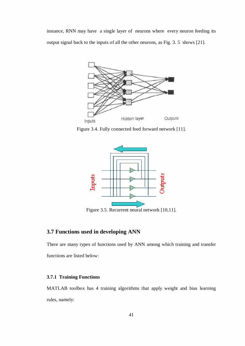
Table 2.3. details the soil types in TEC-2007 that represent the most common local
soil conditions. Table 2.2. details the local site classes that shall be considered as the
bases of determination of local soil conditions.
Table 2.2. Local Site Classes [9].

11
Table 2.3. Soil Groups [9].
2.2.3 Seismic Design
The spectral acceleration coefficient that is given in equation (2.1) must be
used for determination of seismic loads. The elastic spectral acceleration Sae (T),
which is defined as the ordinate of elastic acceleration spectrum for 5% damped rate
where the elastic acceleration the spectrum is equal to spectrum acceleration
coefficient times the acceleration of gravity"g" as given in equation (2.2).
(2.1)
(2.2)

12
where :
Effective ground acceleration coefficient,
I : Building importance factor,
S(T) : Spectrum coefficient,
Sae(T) : Elastic spectral acceleration,
g : Gravitational acceleration .
Table 2.4 details the effective ground acceleration coefficient (A0).
Table 2.4. Effective Ground Acceleration Coefficient [9].
Seismic Zone . A0
1 0.4
2 0.3
3 0.2
4 0.1
(2.3)
(2.4)
(2.5)
The spectrum characteristic periods, TA and TB, are specified in Table 2.5.
Table 2.5. Spectrum Characteristic Periods [9].

13
Spectrum characteristic periods that are defined in Table 2.5 for local site class Z4
must be used in case where previous requirements are not met. In some cases, the
elastic acceleration spectrum can be defined by special investigations via considering
local seismic and site conditions.
Figure 2.1. Design Acceleration Spectrums [9].
In order to consider the specific nonlinear behavior of the structural system during
earthquake, the elastic seismic loads are determined in terms of spectral acceleration
coefficient by dividing to the seismic load reduction factor. Where seismic load
reduction factor, must be calculated according to equations (2.6) or (2.7) based on
the structural system behavior factor, "R" is detaled in Table 2.6 and defined for
various structural systems, and the natural vibration period T.
(2.6)
(2.7)
Ra(T) : Seismic Load Reduction Factor.

14
Table 2.6. Structural Systems Behavior Factors [9].

15
2.2.4 Definition of Load Combination According to TEC-2007
The following combinations are used to determine the design value for the action
of seismic design situation:
In the case of unfavorable result, the below equations should be used
16
Table 2.7 shows Live load participation factor (n). This n must be taken as 1 in
industrial buildings. 30% of snow load shall be considered for the calculation of roof
weight for seismic load.
Table 2.7. Live Load Participation Factors [9].
2.2.5 Methods of Analysis
There are three methods used for the seismic analysis of buildings which are :
1 Equivalent Seismic Load Method
2 Mode - Superposition Method.
3 Time Domain Method.
2.2.5.1 Equivalent Seismic Load Method
Equation 2.13 is selected to determine the total equivalent seismic load (base shear),
"Vt", acting on the whole building in the direction of earthquake (TEC, 2007).
where:
Vt : total equivalent seismic load acting on the building,
T1 : The first natural vibration period of the building,
W : Total weight of the building,

17
A : Spectral Acceleration Coefficient,
Ra : Seismic Load Reduction Factor,
Ao : Effective Ground Acceleration Coefficient,
I : Building Importance Factor.
Total building weight "W", that used in Equation 2.13 as the seismic weight must be
calculated according to Equation 2.12. Total equivalent seismic load determined by
Equation 2.13 is expressed by Equation 2.14:
Additional equivalent seismic load, , acting at the N'th storey (top) must be
calculated by using Equation 2.15 (TEC, 2007).
Excluding , remaining part of the total equivalent seismic load must be
distributed to stories by Equation 2 .16 (TEC, 2007).
where:
Fi : Design seismic load acting at i'th storey,
Wi : Weight of i'th storey,
Hi : Height of i'th storey .

18
2.2.5.2 Mode Superposition Method
In Mode Superposition method displacements and maximum internal forces are
calculated by the statistical combination of maximum contributions obtained from
each of the sufficient number of natural vibration modes considered (TEC, 2007).
2.2.5.3 Analysis Methods in Time Domain
In this method artificially generated and recorded earthquake ground motions can be
used in both the linear or nonlinear seismic analysis of buildings in the time domain.
2.3. Performance Analysis According to TEC-2007
Performance based design helps describing the inelastic behavior of the structural
component of a building. By this approach the actual behavior of a building can be
estimated more accurately during a specified ground motion. Since all the structural
members are examined individually in performance design procedures, it is easy to
see which member or member group does not satisfy the desired performance level.
This design technique has two main parameters one is the demand which represents
the ground shaking motion that affects to the structure; the other is the behavior of
the structure under this ground shaking motion which can be named as capacity of
the structure.
2.3.1. Limits of Damage in Construction Elements and Areas of Damage
2.3.1.1. Damage Limits in Cross Sections
On the cross section for ductile element there are three limit conditions which are
Minimum Damage Limit (MN), Safety Limit (GV) and Collapsing Limit (GÇ).
Minimum damage limit defines the starting of the behavior beyond elasticity, safety
limit can be defined as the limit when the section behavior be beyond elasticity and

19
able to the strength safely, collapsing limit is the behavior limit before collapsing.
This classification invalid for elements damaged in a brittle case.
2.3.1.2. Sectional Damaged Areas
Elements that the damages with critical sections do not reach MN are within the
Minimum Damage Region, those in-between MN and GV are within Marked
Damage Region, those in-between GV and GÇ are in Advanced Damage Region, and
those going beyond GÇ are within Collapsing Region as detailed in Figure 2.2 [9].
2.3.1.3. Definition of Damages in Cross Sections and Elements
Damage regions that cross-sections belong to, shall be decided according to the
comparison of the internal forces and / or deformation calculated using linear or
nonlinear methods with the numerical values corresponding to cross section damage
limits described in section 2.1.1. Damage of the element shall be decided according to
the cross section of the element that with greatest damage.
Figure 2.2. Member damage levels and member performance regions on
capacity curve [9].

20
2.3.2. Building Performance Levels
Seismic safety of the buildings is related to the damage level possibly to occur in the
structure under effect of the seismic load applied. Four building performance levels
are defined.
2.3.2.1. Immediate Occupancy Level (HK)
The building can still be considered ready for use (Immediate Occupancy Level)if at
most 10 % of the beams in this building exceed the Marked Damage Region
Significant Damage Zone and all other elements remain in the Minimum Damage
Zone.
2.3.2.2. Life Safety Performance Level (CG)
The buildings that live up to the conditions provided below that can be agreed to be
in the Life Safety Performance Level, if there are any, are strengthened:
(a) As a result of the calculations made for each direction that the earthquake takes,
applies on each floor, at most 30 % of the beams except for the secondary ones
(which does not take place in the horizontal load-bearing system) at most, the
proportion of the columns defined in paragraph (b) can be in the Advanced Damage
Zone.
(b) The total contribution of the columns in the Advanced Damage Zone to the shear
force that is borne by the columns in each floor should not exceed 20 %. The ratio of
total shear force of the vertical components in (Advanced) significant damage region
at roof story to total shear force of the columns at the related story ratio can not be
more than 40 %.

21
(c) All the other loads – which bear components in the Minimum Damage Zone or
Marked Damage Zone. However, the ratio of the shear force carried by the columns,
exceeding the minimum damage limit in both upper and lower end sections at any
story, to the shear force carried by all columns at the related story ratio must be less
than 30 %.
2.3.2.3. Collapse Prevention Level (GÖ)
The buildings that live up to the conditions provided below, are agreed to be in the
Collapse Prevention Level supported by the fact that all components that are brittle
damaged are in the Collapse Zone.
(a) The results of the calculations concerning all earthquakes that can be applied to
any of the floors. At most 20 % of the beams except for the secondary ones (that
does not take place in the horizontal load-bearing system) can enter the Collapse
Zone.
(b) All other load-bearing components are placed in the Minimum Damage Zone,
Marked Damage Zone or in the Advanced Damage Zone. However, the ratio of the
shear force carried by the columns whose minimum damage limits are exceeded in
both upper and lower end sections at any story to the shear force carried by all
columns at the related story ratio must be less than 30 %.
(c) The building usage under the mentioned circumstances threatens the safety of
nearby human life and populace.

22
2.3.2.4 Collapse Level (GÇ)
If the building does not provide the conditions of collapse prevention level, it can be
considered as in Collapse Level. The usage of the building in existing condition is
not permitted.
2.3.3. Targeted Performance Levels for The Buildings
Three types of ground shaking are defined to be taken into consideration in
performance based design and evaluation. These ground shakings are explained by
having probabilities to be exceeded in 50 years.
Service (Usage) Ground Shaking: It is defined as ground shaking having a 50 %
probability to be exceeded in 50 years. Return period of this ground shaking is
approximately 72 years. The effect of this ground shaking (spectral acceleration)
is half of the effect of ground shaking defined below.
Design Ground Shaking: It is defined as ground shaking having a 10 %
probability to be exceeded in 50 years. Return period of this ground shaking is
approximately 475 years. This ground shaking is used in the Turkish Earthquake
Codes 1998 and 2007.
The Biggest Ground Shaking: It is defined as ground shaking having a 2 %
probability to be exceeded in 50 years. Return period of this ground shaking is
approximately 2475 years. The effect of this ground shaking is 1.5 times of the
effect of design ground shaking.

23
Table 2.8. Minimum Building Performance Targets Anticipated for Different
Earthquake Levels [9].
2.3.4. Determining the Building Performance in Earthquake with Linear Elastic
Performance Analysis Method
Linear elastic calculation methods to be used for the determination of seismic
performances of buildings are the calculations methods defined in 2.2.5. Additional
rules as stated below shall be applied concerning these methods.
Equivalent seismic load method using if the total building height is less than 25m
and 8 storey as well as have buckling disorder calculated without
considering joint eccentricity. Equation (2.13) is used for calculation of total
equivalent seismic load (ground shearing force) where Ra=1 is taken and right side of
the equation is multiplied with factor. = 1.0 in one or two storey structures except
cellars and in others be 0.85. When using the Mod Combination Method, in the
Equation (2.18) Ra=1. In calculations of internal forces and elements capacities

24
which are adaptable to applied seismic direction, internal force directions obtained in
the mode that is dominant in this direction shall be based.
: Acceleration spectrum ordinate for the natural vibration mode [m /s2],
: Elasticity spectrum ordinate [m /s2],
: Seismic Load Reduction Factor.
2.3.4.1. Determination of Damage Level in the Structural Elements of
Reinforced Concrete Buildings
In the description of damage boundaries of ductile elements with linear elastic
calculation methods, numerical values figured as (r) shall be used in the effect /
capacity ratios of beams, column and wall elements and sections of strengthened
masonary filled walls. Reinforced concrete elements are classified as “ductile” if
their fracture type is under bending and “brittle” if it is under shearing effect.
a) In order the beams, columns and walls to be considered as ductile element,
Shearing force calculated in accordance with the bending capacity in the critical
sections of those element should not exceed the shearing capacity calculated
according to TS - 500. On the calculation of Ve for columns, beams and walls,
bearing force moments shall be used. In case the total shearing force calculated with
gravity loads by taking Ra= 1 is less than Ve, then this shearing force shall be used
instead of Ve.

25
b) In order the beams, columns and walls to be considered as ductile element also it
is necessary to provide condition.
: Total height of partition,
: Length of partition.
c) Reinforced concrete elements that are not provide the conditions for ductile
element given in (a) and (b) are defined as brittle damaged elements. Effect /
capacity ratio of ductile beam, column and wall sections is determined by dividing
the section moment calculated under seismic load by taking Ra= 1 to over moment
capacity. On the calculation of effect / capacity direction of the applied earthquake
must be taken into account.
a) Over moment capacity of section is the difference between bending moment
capacity of the section and moment effect calculated on the section under gravity
loads. Moment effect calculated under gravity loads in the supports of the beam can
be reduced maximum 15 % according to retransfer principle.
b) Effect / capacity ratios of column and wall sections can be calculated in such a
way as defined in TEC-2007 in Information Annex 7A.
Effect / capacity ratio of strengthened filled walls are the shearing force strength of
shearing force calculated under the effect of earthquake. Shearing forces formed in
the strengthened filled walls which are modeled with diagonal bars shall be taken
into consideration as the horizontal concurrent of the axial force of the bar.
Calculation of shearing force strength of the strengthened masonnary filled walls is

26
given in TEC-2007 in Information Annex 7F. It is decided that the elements are
located in which damage zone by comparing effect / capacity ratio of beam, column
and wall sections and strengthened filled walls (r) with boundary values given in
Table 2.9 - 2.12. Besides, on the determination of damage zones of strengthened filled
walls in the reinforced concrete buildings boundary ratios of relative storey drift
given in Table 2.12 shall also be taken into consideration. Ratio of relative storey
drift shall be obtained by dividing the maximum relative storey drift to storey height.
For intermediate - values given in Table 2.9 - 2.12 linear interpolations shall be
applied.
Table 2.9. The effect / capacity ratios (r) defining the boundary of the damage for
reinforced concrete beams [9].

27
Table 2.10. The effect / capacity ratios (r) defining the boundary of the damage for
reinforced concrete columns [9].
Table 2.11. The effect / capacity ratios (r) defining the boundary of the damage for
reinforced concrete walls [9].
Table 2.12. The effect / capacity ratios (r) defining the boundary of the damage for
strengthened filled walls and ratios of relative storey drift [9].
2. 3.4.2. Control of Relative Storey Drifts
In the calculation made with linear elastic methods in each earthquake direction,
relative storey drifts of columns, beams or walls in each storey of the building should
not exceed the value given in Table 2.13. where indicates the relative storey drift
calculated as a replacement difference between bottom and top ends of the j’th
column or wall in i’th storey whereas hji indicates the height of the relevant element.

28
Table 2.13. Boundaries of Relative Strorey Drift [9].
2.3.5. Determining the Seismic Performance of the Building using Nonlinear
Analysis Methods
2.3.5.1. Definition of Nonlinear Analysis Method
The aim of the non–linear analysis methods to be used in determination of structural
performances and retrofitting analysis of existing buildings under the effect of the
seismic loads, is calculating the plastic rotation demands of ductile behavior and the
demand for internal forces of brittle behavior for a given earthquake. Then, these
demand values are compared with deformation capacities defined in this section.
Evaluation of the structural performance is done for the performance level of the
member and the building. The non-linear analysis methods are:
Incremental Equivalence Seismic Load Method,
Incremental Mode Combination Method,
Measurement within the Scope of Time Definition Method.
First two are the methods that shall be used for the Incremental Repulsion Analysis
(Pushover Analysis) that is taken as a basis for determining the non - linear seismic
performances and for the strengthening measurements.
2.3.5.2. Methodology of Pushover Analysis Method
The steps that should be followed in the inelastic non-linear performance evaluation
conducted applying the Pushover Analysis are summarized below.
(a) In order to idealize the non-linear behavior of the load-bearing system and build
the analysis model the rules defined in 2.3.5.3 must be followed.

29
(b) A non linear static analysis in which the vertical loads that are in accordance with
the masses are taken into account must be conducted before applying the pushover
analysis . The results of this analysis must be using as the primary conditions of the
pushover analysis.
(c) In case the incremental pushover analysis is conducted by applying the
Incremental Equivalence Seismic Load Method, the “modal capacity diagram”
belonging to the primary (dominant) mode the coordinates of which are defined as
“modal displacement – modal acceleration” shall be derived. Modal capacity
diagram obtained at the end of pushover analysis and elastic response spectrum are
taken into consideration together and modal displacement demand of first mode will
be calculated. At the last step, displacements which refer the modal displacement
demands, plastic deformations (plastic rotations) and internal force demands will be
evaluated.
(d) From the plastic rotational demands which are calculated for the ductile sections,
the plastic curvature demands will be evaluated which will handle to find the total
plastic curvature demand of the member. After that, in accordance with these the
strain demands for the concrete and reinforcement steel will be achieved for
reinforced concrete members. These strain demands will be compared with the strain
limits which are specified for different damage levels so a performance level
evaluation will be done in sectional for structural members in ductile manner. Also
the obtained shear force demands will be compared with the shear capacity of
sections to make a consideration in brittle manner.

30
2.3.5.3. Idealizing the Inelastic Non-linear Behavior
In this specification, it is suggested to use “elastic perfectly plastic hypothesis” for
nonlinear analysis. It is assumed that plastic deformations occur uniformly
distributed within the plastic hinge length. In case of simple bending, length of the
plastic deformation region called plastic hinge length shall be taken as equal to
half of member dimension in bending direction (h) .
(2.18)
It is required that plastic hinges are located in the exact middle of the plastic
deformation region theoretically. But in practical operations, following approximate
idealizations can be allowed:
(a) In Plastic hinges shall be located at sufficient distance from the column-beam
connection region. But, it must be considered that plastic hinges can occur at spans
of the beams due to vertical loads.
(b) In reinforced concrete shear walls, plastic hinges are allowed to be assigned in
bottom ends of shear walls in each story. U, T, L or box typed shear walls, must be
idealized as single shear wall sections. In the case of basement floors of the buildings
are encircled by rigid shear walls, plastic hinges of these shear walls going towards
the upper floors must be located by starting on basement.

31
(c) Yield surfaces of the reinforced concrete members can be modeled as yield lines
and yield planes for two dimensional and three dimensional behavior conditions
respectively.
2.3.5.4. Pushover Analysis Using Incremental Equivalent Seismic Load Method
In incremental equivalent seismic load method, nonlinear pushover analysis is
performed under monotonically increasing equivalent earthquake load until
performance point is reached. Performance point is also named as target modal
displacement demand. Displacement, plastic deformation, increase in internal forces
and related cumulative values are determined at each pushover step. Once the system
reaches its performance point, total base reaction and roof displacement values are
determined. Performance point is also named as target modal displacement demand.
To be able to use the Incremental Equivalent Seismic Load Method, it is required
that; the effective mass calculated by considering first natural vibration mode of
considered earthquake direction to total building mass shall not be less than 0.70 and
torsional irregularity coefficient calculated without considering additional
eccentricities is . In addition, number of stories shall not be more than eight
excluding basement.
During incremental Pushover Analysis, the distribution of the equivalent seismic
load can be assumed to remain constant, independent of the plastic section
formations in the load-bearing system. In such a case, load distribution shall be
determined in a way that it shall be proportional to the value derived by multiplying
the natural vibration mode shape magnitude of the primary (dominant in the seismic
direction) that is computed for the linear elastic behavior at the first step of the

32
analysis with the magnitude of the related mass. In the buildings where floor slabs
are idealized as rigid diaphragms, two perpendicular horizontal drifts in the center of
mass of each floor and the rotation around the vertical axis passing through the
center of mass shall be considered as the magnitudes of the primary (dominant)
natural vibration mode shapes.
By means of the repulsion analysis (Pushover Analysis ( conducted in accordance
with the constant load distribution the repulsion curve the coordinates of which are
“top translocation – ground shear force” shall be obtained. Top translocation is the
translocation that is calculated in each repulsion step and that takes place in the
center of mass of the top floor of the building for the earthquakes in the direction x
that are taken into consideration. And the ground shear force is the sum of the
equivalent seismic loads of each step for the earthquake in the direction of x.
2.3.5.5. Pushover Analysis with Incremental Mode Combination Method
The aim of the Incremental Mode Combination Method is incrementally
implementing the Mode Combination Method taking modal translocations that are
gradually and monotonically increased in a way that shall be proportional to the
sufficient number of natural vibration mode shapes representing the load-bearing
system behavior and that are scaled in a way that they shall be in harmony with each
other or taking the modal seismic loads that shall be in harmony with the mentioned
modal. Such Pushover analysis method that is based on the “step by step linear
elastic” behavior in the load - bearing system for each repulsion step between the
formations of two sequential plastic sections is explained.

33
2.3.5.6. Calculation with the Non-linear within the Scope of Time Definition
Method
Analysis Method in Time Domain is step by step integration of the movement
equation of the system by considering non–linear behavior of the structural system.
The displacement, deformation and internal forces occur in the system in the duration
of the analysis in each time increase and the maximum equivalent values of them
with respect to the seismic demand are calculated.

34
Chapter 3
ARTIFICIAL NEURAL NETWORKS
3.1 Introduction
Artificial Neural Networks (ANN) are commonly used to solve the the problems that
might be complicated or there are difficult in modeling by using other techniques like
mathematical modeling [10,12,13]. ANN are used in many problems in structural
engineering.
This chapter exhibits the fundamentals of Artificial Neural Networks showing the
history, definition, terminology used, as well as advantages and disadvantages. The
mechanism of ANN, architecture classes, algorithms used for training are also
reviewed. Finally, several applications of ANN used in civil engineering are
included.
3.2 Definition of Artificial Neural Networks
Artificial Neural Network (ANN) is an assembly (network) of a large number of
highly connected processing units, the so-called nodes or neurons. The neurons are
connected by connections. The strength of the connections between the neurons is
represented by numerical values (weights) [13,14,15].

35
3.3 Terminology used in Artificial Neural Network
The definitions of the terms that showed in Figure 3.1 are given in the following
paragraphs:
Figure 3.1. Typical Structure of ANN [11]
Neuron (artificial): It has inputs from other neurons, with each of which is
associated a weight - that is, a number which indicates the degree of importance
which this neuron attaches to that input, and it is also called nodes [16,17].
Weight: A parameter associated with a connection from one neuron, A, to another
neuron B. Weight determines value of notice the neuron B pays to the activation it
received from neuron A [17].
Output
Inputs First Hidden Second Layer
layer Hidden Layer

36
Input unit: It is a neuron without input connections. And its activation thus comes
from outside the net [17].
Output unit: It is a neuron without output connections. And its activation thus
represent the output value of the net [17].
Bias: In some neural networks like feed-forward, every hidden unit and every output
unit is connected by a trainable weight to a unit (the bias unit) that always has an
activation level of -1[17].
Epoch: Number of times of training. Usually it used as a measure the learning speed
as in "the training has been completed after n epochs" [17].
Hidden layer: Layers that between the input and output layers (layers that consist of
hidden neurons) are called hidden layers [17].
Hidden unit / node: It is a neuron that is not an input unit or an output unit [17].
A learning algorithm is a procedure for adjust the weights [12].
Note: The back-propagation consider the most widely used and successful learning
algorithm used in training multilayer neural networks [12].
3.4 Advantages and Disadvantages of ANN
Artificial neural networks have many advantages that make a lot of researchers to
apply it in their studies. Some of those advantages are:

37
1- Artificial neural networks can model some complex problems where the
relationships that connect the model variables are unknown [12], [10].
2- ANN can producing correct or nearly correct result (outputs) when the presented
inputs be partially incorrect or incomplete [14], [10].
3- It is not necessary to have prior knowledge about the relationship that connect
between the input/output, and this is one of the benefits that neural networks
distinguishes from other statistical and empirical methods . [12], [10].
4- Artificial Neural Networks can be updated for getting a better result via adding
new training examples to the network [11], [10].
5- ANN can give the outputs without performing manual works like using equations,
charts, or tables [15], [12].
6- Using neural networks is faster than a conventional approaches [16], [12].
7- ANN are applicable for dealing with noisy and incomplete data [18], [12].
8- ANN have the ability to learn and generalize form previous examples to produce
solutions for different problems [18], [12].
9- Experimental data, theoretical data, empirical data can be presented to ANN for
training based on reliable experiences [18], [12].

38
Although the advantages of neural networks, from another side they have also
disadvantages. Some of them are :
1- They give results without explaining how they get solutions. The accuracy of
ANN depends on the quality of the trained data and the capability of the user to
choose reliable representative inputs [10].
2- There is no exact formula to determine the architecture of ANN and which
training algorithm shall be used in a given problem. Trial and error is the best
proposal solution . User can get an idea via examining the problem then deciding to
start with simplest network; going on to complex ones until getting a good solution
that is withen the acceptable limits of error [10].
3- The model tends to be like a black box because the relations that link between
inputs and outputs did not develope by the judgment of the engineer or the user [10].
It seems that the advantages of ANN outweigh the disadvantages [10].
3.5 Mechanism of Artificial Neural Networks
Neural networks are composed of simple elements that operating in parallel. The
function of network can be determined in general by the connections between
elements. Neural network can be trained to perform a specific function via adjusting
the values of the connections (weights) that are connect between the elements.
As shown below in Fig 3.2. , the network is adjusted, based on a comparison of the
output and the target frequently until the output of the network matches the target.

39
Figure 3.2. The Concept of Neural Networks [11].
3.6 Types of Artificial Neural Networks
Artificial neural networks can be classifyied according to the connection geometries.
Feed-forward network is one of the most simple architectures [20].
3.6.1 Single-Layer Feed Forward Networks
The neurons in a layered neural networks are organized in layers. The simplest shape
of a layered network consist of an source nodes (input layer) which projects into an
computation nodes (output layer), but not vice versa. In other words, this kind of
networks are feed forward or in one way. As Fig. 3.3 shows. This network is called
a single-layer network, "single-layer" refers to the output layer .Since no
computation is performed in the input layer it is not counted [21].
Figure 3.3. Feed forward network with a single layer of neurons [11].

40
3.6.2 Multi-Layer Feed Forward Networks
This type of neural networks has at least one hidden layer, where the computations
dose also called hidden neurons. The main function of hidden layer is to intervene
between external inputs and the outputs of network in a useful manner as detailed in
Fig 3.4.
Fig. 3.4 shows the layout of a multilayer feed forward neural network with one
hidden layer. This network for brevity can be referred to as a 6-4-2 network since it
has 6 source neurons, 4 hidden neurons, and 2 output neurons [21].
In Fig. 3.4, the neural network is fully connected, which implies that every node in
every layer is connected to each other node in the adjacent forward layer. If some of
the (synapticlconnections) were missed then the network can be considered partially
connected [21].
3.6.3 Recurrent Neural Networks
The difference between recurrent neural network and feed forward neural network is
that, the first one has one feedback loop at least. In the network topology Recurrent
Neural Network (RNN) has a closed loop. Basically, RNN developed in order to
deal with the time varying or time-lagged patterns. Also they are commonly used
when the dynamics of the process the problems is complex or having noisy data.
The Recurrent Neural Network can be fully or partially connected. All the hidden
units in fully connected type are connected recurrently, on the other hand, the
recurrent connections in the partially connected RNN are omitted partially. For
41
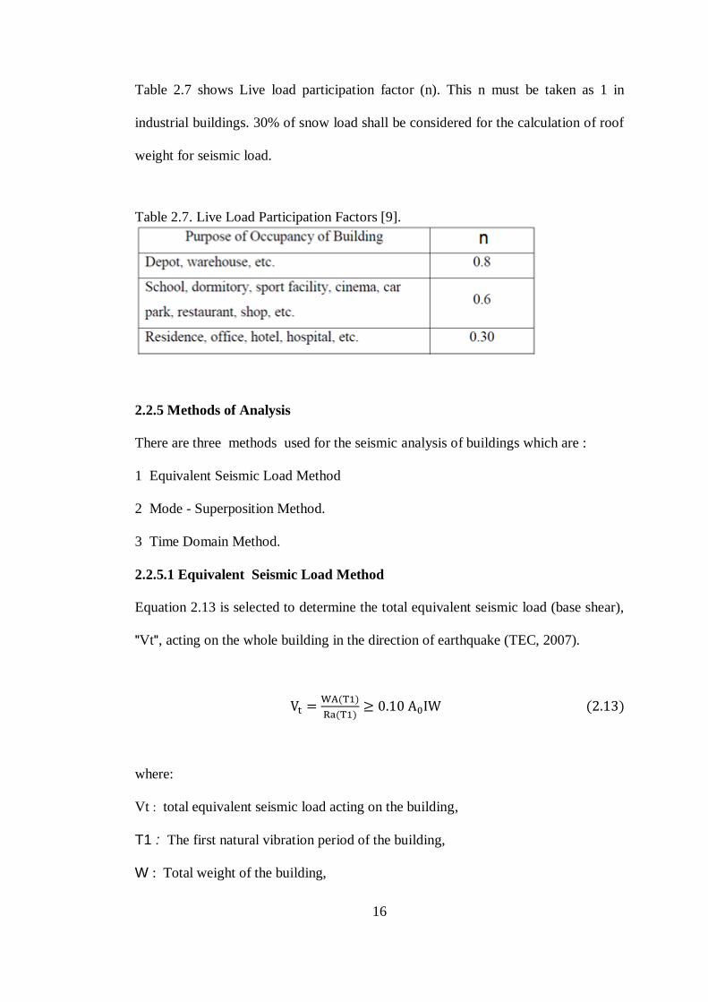
instance, RNN may have a single layer of neurons where every neuron feeding its
output signal back to the inputs of all the other neurons, as Fig. 3. 5 shows [21].
Figure 3.4. Fully connected feed forward network [11].
Figure 3.5. Recurrent neural network [10,11].
3.7 Functions used in developing ANN
There are many types of functions used by ANN among which training and transfer
functions are listed below:
3.7.1 Training Functions
MATLAB toolbox has 4 training algorithms that apply weight and bias learning
rules, namely:

42
Batch training function “trainb”.
Cyclical order incremental training function “trainc”.
Random order incremental training function “trainr”.
Sequential order incremental training function “trains” [11].
3.7.2 Transfer (Activation) Functions
An activation function is the function that describes the output behavior of a neuron.
Activation functions can be linear or nonlinear [11]. Fig 3.6. shows the most three
commonly used functions which are :
Hard-Limit Transfer Function.
Linear Transfer Function.
Log-Sigmoid Transfer Function.
-Neurons of Linear Transfer Function shown Fig. 3.6 are used as linear
approximations in “Linear Filters”.
- The sigmoid transfer function shown in Fig. 3.6 takes the input and squashes the output
into the range 0 to 1. [11].
3.8 Algorithms used for Training Artificial Neural Network
There are several types of neural networks according to algorithms used in the
training process. The following paragraphs presents some of these training
algorithms :

43
Figure 3.6. Three of the most commonly used transfer functions[11]
3.8.1 Back-propagation Neural Networks
The most popular type of neural networks is the back propagation neural network
(BP). Back-Propagation is a mathematical procedure that starts with the error at the
output of a neural network and propagates this error backwards through the network
to yield output error values for all neurons in the network. BP is a feed forward
network that uses supervised learning to adjust the connection weights. In a feed
forward network, the results of each layer are fed to each successive layer. A
conventional BP uses three layers of nodes, but it can use more middle layers. The
first layer, the input nodes, receives the input data (also called the middle layer or the

44
hidden layer). The results of the first layer are passed to the next layer. This process
is repeated for each layer until an output is generated. The difference between the
generated output and a training set output is calculated. This difference is fed back to
the network where it is used for connection weight readjustment by iteratively
attempting to minimize the difference to within a predefined tolerance. The BP can
learn many different output patterns simultaneously with dramatic accuracy [11,11].
3.8.2 Radial Basis Neural Networks
Radial Basis Functions are powerful techniques for interpolation in multidimensional
space. A Radial Basis Function (RBF) is another type of feed-forward ANN as
showen in Fig 3.7. Typically in RBF network, there are three layers: one input, one
hidden and one output layer. Unlike the back-propagation networks, the number of
hidden layer can not be more than one. The hidden layer uses Gaussian transfer
function instead of the sigmoid function. In RBF networks, one major advantage is
that, if the number of input variables is not too high, then learning is much faster than
other type of networks.
Figure 3.7. Architecture of radial basis function neural network [11].

45
3.8.3 Hopfield Neural Networks
Hopfield network is the recurrent neural network that has no hidden units. The
concept of this type of networks is to gain a convergence of weights to find the
minimum value for function of energy. Each neuron in the Hopfield network is
connected with all other neurons except itself, therefore the flow does not going in
one way. Even a node can be connected to itself in a way of receiving the
information back through other neurons [22, 24].

46
Chapter 4
METHODOLOGY
4.1 Introduction
This chapter deals with modeling of earthquake performances of reinforced concrete
buildings using artificial neural networks. The reliability of the data collected used in
this research and definition of parameters considered in the study (parameters
affecting on earthquake performance of RC buildings) which represent the input of
the data collected have been explained. The preprocessing which applied on the
collected experimental results is explained.
This chapter also presents the adopted training process to develop a trained neural
network model; the training process includes defining the topology of the required
neural network and identifying all neural network parameters.
The following methodology will be adopted to in this study:
1- Dozens of models of buildings will be carried out for getting database to be used
in training the neural network then testing the results.
2- Effective parameters on earthquake performance will be investigated using
Artificial Neural Network (ANN) and then will be sorted according to their
significances.

47
4. 2 Case Study
In this study, collected total of 260 reinforced concrete buildings with 4 storey, that
were chosen to represent the existing RC buildings. The commercial program
STA4cad is used for modeling and analysing these buildings. The performance
analysis of these 260 RC buildings have listed in the Appendix that were used for
training neural networks. The parameters that affect on earthquake performance
represent the input and the performance represent the output. The performance
analysis of RC buildings was performed according to both the linear performance
analysis and nonlinear (static pushover analysis) procedures as specified in TEC-
2007 [9]. Performance level details are given in Table 4.1. Fig. 4.1 shows 10
different of buildings models out of 201 residence buildings chosen in this analysis.
Earthquake performance of a RC building is based on several parameters. Table 4.2
indicates these parameters and their variation intervals of the selected 260 buildings
for this study.
Table 4.1. Structural Performance Based on Damage [9].

48
Table 4.2. Parameters considered in the study
Parameter 1 2 3 4
A1-Torsional Irregularity Exist None
A2- Slab Discontinuities Case 1
Ab / A > 1/3 Case 2
Ab / A > 1/3 Case 3
Ab / A > 1/3 None
A3 – Projections in Plan Exist
ax > 0.2 Lx , ay > 0.2 Ly
None
B1- Interstorey Strength Irregularity (Weak
Storey).
[ηci = ( Ae)i / ( Ae)i+1 < 0.80]
None [ηci > 0.80]
B2- Interstorey Stiffness Irregularity (Soft Storey)
Exist open ground
storeys >=%50
Exist height difference
between the floors >1.3 times
None
B3 - Discontinuity of Vertical Structural
Elements
Exist None
C2 Weak Column – Strong Beam
Exist None
Stirrup Spacing Ok Not ok
Average Shear Wall Ratio ( )
N/A
0%
0.01 %
Average Column Ratio ( CA)
0.000 % 0.02 %
Concrete Compression Strength (C)
20 25
Type of steel 220 360
Soil Type (Z) Z1 Z2 Z3 Z4
Code 2000 1990 1901
Earthquake zone (EZ) 0.4 0.3 0.2 0.1
Importance Factor (I) 1 1.2 1.4 1.5
Structural Performance (S1-S4)
S1 S2 S3 S4

49

50

51
Figure 4.1. Ten different plans of building models used in this study

52
4.3 Definition of Parameters Affecting on Earthquake Performance
of RC Buildings.
(1 Number of Storey (NS)
This study deals with RC buildings with 4 storey only.
2) A1-Torsional Irregularity
Torsional irregularity is the first type of irregularity in TEC-2007 and called A1-
type irregularity. Torsion in buildings is resulting from the asymmetrical distribution
of rigidity. The case where Torsional Irregularity Factor, bi, which is defined as the
ratio of the maximum drift at any storey to the average storey drift at the same storey
in the same direction, is greater than 1.2, as shown in Figure 4.2.
Figure 4.2. Type A1- Torsional Irregularity [9].
In this case the behaveior of floors are assumed to be rigid diaphragms:
(4.1)
(4.2)

53
where;
bi : Factor of torsional irregularity for i,th storey,
(i)ort : Average storey drift of i,th storey of the building,
(i)max : Maximum storey drift of i,th storey of the building,
(i)min : Minimum storey drift of i,th storey of the building.
Storey drifts shall be calculated by considering the effects of ± %5 additional
eccentrics [9].
In particular, it is quite difficult to determine Torsional Irregularity and in rapid
assessment methods, it is selected based on engineering judgment, in this study
Torsional Irregularity have been checked by Sta4cad software in order to be sure
about the effect of Torsional Irregularity on earthquake performance.
3) A2-Floor Discontinuities
"Floor Discontinuities" is the second type of irregularity are called" A2-type
irregularity". There are 3 cases of floor discontinuity irregularities that may occur in
any floor:
First case where the area of the openings in any floor exceeds 1/3 of the total
gross area, as shown in Figures 4.3 (a) and (b).

54
Type A2-Irregularity-I (b) Type A2-Irregularity-I
Figure 4.3. Type A2- Floor Discontinuity Cases I [9].
(4.3)
(4.4)
where;
Ab : Total area of openings
A : Total gross area of the floor
Second cases where openings in the floor lead a difficult transfer of seismic loads
safely to vertical elements in the structur, as shown in Figure 4.4 (a) and (b).
(a) Irregularity-II (b) Irregularity-III
Figure 4.4. Type A2- Floor Discontinuity Cases II [9].
The third case having reductions in the in-plane strength and stiffness of floors.

55
4) A3- Projections in Plan
This type of irregularity called "A3-type of irregularity". The cases where
projections beyond the re-entrant corners exceed the total plan dimensions by more
than 20%. There are three drawings explaining this irregularity are shown below:
Figure 4.5. Type A3- Irregularity [9].
(4.5)
(4.6)
where;
: Length of the building at x, y direction,
: Length of re-entrant corners in x, y direction,
5) B1- Interstorey Strength Irregularity (Weak Storey).
This type of irregularity called "B1-type " in TEC-2007. In each of the orthogonal
earthquake directions, the case where Strength Irregularity Factor ηci, is less than
0.80 , where ηci is the ratio of the effective shear area of any story to the effective
shear area of the story immediately above. B1-type is commonly exist in the ground
floors of the commercial buildings.
ηci = (Ae)i / (Ae)i+1 < 0.8 (4.7)

56
where;
Ae : Effective shear area.
Definition of effective shear area in any storey:
Ae = Aw + Ag + 0.15 Ak (4.8)
where;
Aw : Effective of web area of the column cross sections,
Ag : Section areas of structural elements at any storey,
Ak : Infill wall areas.
6) B2- Interstorey Stiffness Irregularity (Soft Storey)
This type is called B2-Type of irregularity. In each of the two orthogonal earthquake
directions, the case where stiffness irregularity factor ki is greater than 2.0, where
ki is the ratio of the average storey drift at any storey to the average storey drift at
the storey above or below, as shown in the expression (4.9.a) and (4.9.b) :
ηki = (i/hi)ave / (i+1/hi+1)ave > 2.0 (4.9.a)
ηki = (i /hi)ave / (i -1/hi-1)ave > 2.0 (4.9.b)
where:
ηki: Stiffness irregularity factor defined at i'th storey of the building,
i: Storey drift of i'th storey of the building [m],
hi: Height of i'th storey of building [m].
Storey drifts shall be calculated, by considering the effects of ±%5 additional
eccentricities.

57
Soft Story: It is exists when the stiffness of one story is less than the others. In a rapid
visual screening, it is not possible to quantitatively determine and compare the
stiffness of each story [ 0 ]. Generally in building the ground floor is designed to be
higher than the other floors. Therefore, this causes a difference in stiffness or
rigidity between floors. Also open ground storeys (i.e. shops) cause soft story, while
great storey drift will be in the ground floor, the upper floors move such as a
diaphragm. High stress concentration occurs and maybe leads to collapse the
structure [27],[25]. Certain observable conditions, however, provide clues that a soft
story may exist. If one of these conditions described below exist :
One of the stories has fewer walls or columns (or more windows and openings)
than the floor above it. Length of lateral system at any story is between 50% of
that at story above. Figure 4.6 shows an industrial building with large openings at
the ground floor. These large openings cause the first floor piers to be narrower
than the piers at upper stories resulting in a weak story. This is considered as
sevare vertical irregularity[6].
Figure 4.6. Illustration of a building with a soft ground story due to large
openings and narrow piers.

58
One of the stories is particularly tall compared to the other stories (height of any
story is between 1.3 and 2.0 times the height of the story above). Figure 4.7
shows a building with a ground story significantly taller than the stories above.
This difference in story height causes the piers to be taller at the first floor than at
the upper stories resulting in a soft story. This is considered a severe vertical
irregularity [6].
Figure 4.7. Illustration of a building with a soft ground story due to tall piers.
7) B3-Discontinuity of Vertical Structural Elements
In the TEC-2007 this type is called "B3- type of irregularity". This case occur when
the vertical structural elements are removed or when the structural walls are
supported by beams or columns, as shown in Figure 4.8.
Figure 4.8. Type B3- Discontinuities of Vertical Structural Elements [9].

59
8) Weak Column – Strong Beam
When columns are weaker than beams, they cannot prevent the plastic hinge
formations at columns ends. This kind of plastic hinging mechanisms result in high
inelastic deformations at story level and thus instability of the frame system which
may bring the failure. In the database E and NE representing existing or non existing
Weak Column – Strong Beam respectively.
Figure 4.9. Weak Column – Strong Beam
9) Stirrup Spacing
In the database “OK” represents that Stirrup Spacing is according the code
requirements and “NOT OK” represents that Stirrup Spacing is not according the
code requirements.
10) Average Shear Wall Ratio
Shear walls increase strength and stiffness of buildings, which significantly reduces
the lateral sway [28]. There are 3 different parameters used as an indication of the
base shear capacity of the most critical story. These parameters indicating
normalized areas of the members, which are :
Normalized total column area (ntca).
Normalized total wall area in x − direction (ntwa-x).
Normalized total wall area in y − direction (ntwa-y).

60
The total column and wall areas are normalized with the normal floor area. In the
calculation of the parameter, contribution of the partition walls are considered to be
10% of the contribution of the shear walls. The minimum of the normalized lateral
strength indexes for walls calculated in the two orthogonal directions (ntwa-x, ntwa-
y) from the following equations and the smaller value was considered in data.
where;
, : Total cross-sectional area of shear walls in x and y directions,
respectively.
, : Total cross-sectional area of masonary walls in x and y
directions, respectively.
: Normal floor area.
11) Average Column Ratio (CA)
Namely normalized total column area (ntca)
: Total cross-sectional area of columns,
:Normal floor area.
61
12) Concrete Compression Strength (C)
The compressive strength of concrete was considered as 20 MPa, 25 MPa to
represent Concrete Compression Strength of existing buildings.
13) Type of Steel
The yield strength of the steel was selected as 220 MPa, 360 MPa and for
longitudinal and transverse reinforcement in existing buildings.
14) Soil Type (Z)
Table 4.3. details the soil types in TEC-2007 that represent the most common local
soil conditions. Table 4.4. details the local site classes that shall be considered as the
bases of determination of local soil conditions.
Table 4.3. Local Site Classes [9].

62
Table 4.4. Soil Groups [9]
15) Code
Code 1975
Code 1975 was valid for more than 20 years. Therefore, a lot of the existing
buildings were constructed and designed, when this code was in effect. The term
“ductility” was used for the first explicitly in this code. [35]. The seismic zone
coefficient are (0.10, 0.08, 0.06 and 0.04, for Zones I, II, III and IV respectively).
Code 1998
For the seismic zones I, II, III and IV, the effective seismic acceleration coefficient
(Ao) must be taken as 0.40, 0.30, 0.20 and 0.10, respectively,
This code includes ;

63
• Definition of the acceptable structural performance under the design earthquake,
• Quantitative definition of irregularities,
• Definition of the elastic design spectrum [35].
Code 2007
After 1999 Marmara Earthquake, it is seen obviously that the existing earthquake
code is not adequate to figure out the seismic performance of the existing buildings.
To understand the performance levels of the buildings and to take precautions for the
earthquake in terms of retrofit strategies the earthquake code was revised. The new
code which includes the performance based design was published at 06.03.2007 and
also partially revised at 03.05.2007. This section of the study states the information
of the performance based design according to TEC 2007. Most recent versions of
codes for the seismic design published after 2007 includes a part about seismic
safety assessment of existing buildings and retrofitting [9] [35].
16) Seismic Zone (EZ)
Fig.4.10 shows the current seismic risk map of Turkey. Zone 1 represent highest
risk, while Zone 4 having minimum seismic risk.
Figure 4.10. Seismic Hazard Zonation Map of Turkey [35].

64
Table 4.5 shows the effective seismic acceleration coefficient (Ao) for the seismic
zones.
Table 4.5. Effective Ground Acceleration Coefficient (Ao)
17) Building Importance Factor (I)
Table 4.0. Building Importance Factor ( I ) [9].
4.4 Matlab Neural Network Toolbox
The neural network toolbox is available in MATLAB 2115 Version 8.3 was used in
this study to build the ANN model. Neural network algorithms in MATLAB 2115

65
Version 8.3 can be quickly performed, and wide range of problems can be tested
easily.
4.5 Construction of ANN Model
By applying the preprocessing criteria, it was thought that a reliable training set of
data was obtained. The following sections explain the details of the training process
that was followed in this research. Also the validation of the developed ANN model
is discussed.
4.5.1 Training Strategy of the ANN Model
Feed forward back propagation algorithm was chosen after pre-processing the data
has been completed. Back propagation is the most successful and widely used in civil
engineering applications [30,13].
The first step in training is the data scaling.
Sigmoid transfer function usually used in the networks. Upper and lower limits of
output are generally 1 and 0, respectively. Scaling of the inputs between [-1, +1]
helping in improving the learning speed significantly [18]. A simple linear
normalization function between zero and one is:
where S is the normalized value of the variable P, Pmin and Pmax are variable
minimum and maximum values, respectively.

66
The second step in training a feed forward network is to create the network object. A
feed forward network can be created via using the function nntool by using a
graphical user interface (GUI). This interface enable you to:
• Create neural networks,
• Enter the data into the GUI,
• Initialize, train, and simulate networks,
• Export the training results from the GUI to the command line workspace,
• Import the data from the command line workspace to the GUI.
The third step is setting the training parameters:
a) The number of ‘epochs’(number of times of training) affects on the performance.
This number depends on many factors, the most important are :
Number of training data,
Number of hidden layers,
Number of neurons in hidden layers,
Number of dependent output parameters [18].
b) Maximum permissible error.
c) The number of iterations for which the error becomes constant.

67
d) The training status is displayed for every show iteration of the algorithm.
In Back propagation algorithm inside MATLAB the data can be divided into 3
sets: training, validation and testing sets.
The training set is used to reduce the ANN error. The error on the validation set is
monitored during the training process. The validation set error will normally
decrease during the initial phase of training, as does the training set error [13,31].
However, when the network start to over-fit the data, the error on the validation set
will start to increase. When the validation set error increases for a specified number
of epochs, the training is stopped. The test set is used as a further check for the
generalization of the ANN, but it has no any effect on the training.
In this study, data set was devided into three sets : a 01% for training, 15% for
validation and 15% for testing [13].
The final step is plotting the training progress and the correlation coefficient “r”.
The training process of ANN is presented in a flow chart in Fig 4.11.

68
Figure 4.11. Flow chart for training process of neural networks [32]

69
4.6 Topology of the developed ANN
Two separate ANN models were trained: one for the linear performance analysis
method, and the second one is the nonlinear static pushover analysis method.
4.6.1 Earthquake Performances ANN Model.
There were 10 input parameters; Torsional Irregularity (A1), Slab Discontinuities
(A2), Projections in Plan (A3), Weak Storey (B1), Soft story (B2), Discontinuity of
Vertical Structural Elements (B3), Weak Column – Strong Beam (C2), Stirrup
Spacing ( cm ), Average Shear Wall Ratio, Average Column Ratio (CA) , Concrete
Compression Strength (C), Type of steel (Fy), Soil Type (Z), Code (1975– 1997-
2007 ), Earthquake zone (EZ) and Importance Factor (I) The output parameter is the
Structural Performance (S1-S4).
After several trials and iterations using MATLAB tools the following topology can
be obtained for the Earthquake Performances of Reinforced Concrete Buildings.
The topology of the network is:
Type of architecture : Multi-layer feed forward
Number of layers (hidden + output): 2
Note : The input layer does not count of source nodes because no computation is
performed there.

70
Table 4.7. Number of Used Neurons and Transfer Functions.
Layer Name Number of Neurons Transfer Function
First hidden layer 11 logsig
Output layer 4 purlin
Training algorithm used: Back probation algorithm
Number of epochs required for training: 1000
Performance function: Mean Square Error (MSE) .
The architecture of ANN model for the Earthquake Performances of Reinforced
Concrete Buildings is shown in Fig 4.12.
Figure 4.12. The architecture of ANN model for Earthquake Performances of
Reinforced Concrete Buildings.

71
4.7 Performance of ANN
The Mean Square Error (MSE) using to monitor the training process. Process of
training will stop when any of the following criteria is satisfied:
When the number of (epochs) reach to the maximum;
When the average training error reach to the target;
The performance has been minimized to the target;
When the validation set error starts to increase [31,18,13].
The progress of the training was examined by plotting the training, validation and
test Mean Square Error (MSE), versus the performed number of iterations, as
presented in Fig. 4.13.
Figure 4.13. Training progress of ANN
The results shown in Fig. 4.13 shows that there is no significant over-fitting occurred
because both of the validation set error and the test set error have similar
characteristics. To insure the adequacy of the trained neural network model, the

72
testing data which has been taken randomly from the whole data is taken and trained
separately.
Fig. 4.14 gives comparisons of the Earthquake Performances from experiments and
those obtained from the trained neural network (a) for 182 training data set and (b)
for 39 validation data set (c) for 39 testing data set.
One can see from this comparisons that, earthquake performance using the trained
ANN model is in good agreement with the experimental results 91% accuracy for
non-linear static pushover analysis method and about 89% accuracy for linear
performance analysis method.
Figure 4.14. Performance of ANN for nonlinear static pushover analysis
method

73
Figure 4.15. Performance of ANN for linear performance analysis method
4.8 Testing of Neural Network Performance
In order to check the ability of ANN model to predicting the earthquake
performance of RC buildings, 10 models of buildings that were not used in the
training network have been used in comparison between the predicted performance
by ANN model and the performance by analysis using (STA4cad) as Table 4.9
shows.
The developed neural network model succeed to predict the earthquake performance
for 9 Buildings correctly.
where :
1: Exist
0: None

74
Table 4.8. Data used in testing the neural network model Parameter 1 2 3 4 5 6 7 8 9 10
A1-Torsional Irregularity
0 1 0 0 1 1 0 0 0 0
A2- Slab Discontinuities
0 0 0 0 0 0 0 0 0 0
A3 – Projections in Plan
0 0 0 0 0 0 0 0 0 0
B1- Interstorey Strength
Irregularity (Weak Storey).
0 0 0 0 1 0 1 0 0 1
B2- Interstorey Stiffness
Irregularity (Soft Storey)
0 0 0 0 1 0 1 0 0 1
B3 - Discontinuity of
Vertical Structural Elements
0 0 0 1 1 0 1 0 0 1
C2 Weak Column – Strong
Beam 0 0 1 0 1 0 1 0 0 1
Stirrup Spacing 1 1 0 0 0 0 0 1 1 0
Average Shear Wall Ratio
( ) 0 0 0 0 0 0 2 2 0 2
Average Column Ratio ( CA)
0.01 0.01 0.01 0.01 0.01 0.01 0.01 0.01 0.0087 0.01
Concrete Compression Strength (C)
20 25 20 20 20 20 20 20 25 20
Type of steel 220 220 220 220 360 360 220 360 360 220
Soil Type (Z) Z2 Z1 Z1 Z1 Z1 Z2 Z3 Z1 Z2 Z1
Code 1975 1997 1975 1975 1997 1975 1975 1997 2007 1975
Earthquake zone (EZ)
0.1 0.3 0.2 0.2 0.2 0.4 0.2 0.4 0.2 0.4
Importance Factor (I)
1 1 1 1 1 1 1 1 1 1
Linear Performance by
STA4cad 1 2 2 3 4 2 3 2 1 4
Non Linear Performance by
STA4cad 1 2 2 2 3 4 1 2 1 4
Linear Performance by
ANN 1 2 2 3 4 2 3 4 1 4
Non Linear Performance by
ANN 1 2 2 2 3 4 1 4 1 4

75
Chapter 5
PARAMETRIC STUDY
5.1 Introduction
The advantage of trained neural network models is that parametric studies can be
easily done by simply varying one input parameter and all remaining input
parameters are set to constant values [34]. In this chapter the effective parameters
on earthquake performance have been investigated by using the trained model of
Artificial Neural Network to determine the most effective parameters on earthquake
performance of RC buildings.
Each one of the parameters have an impact on the seismic performance of buildings,
according to the results of the 260 model analysis, but this effect may be obvious and
significant in some cases and in others it have not shown clear because there is
another factor more important. In order to determine the most parameters affect on
seismic performance of buildings the effect of each parameter on the seismic
performance of the building has been checked separately in three different cases
where the value of each parameter has changed in each case with the stability of the
rest of the parameters in each case. These three cases are:
The first case: In this case, all the parameters are in the lower case with less value or
non-existent, the effect of each parameter on the seismic performance of the

76
building has been checked separately to determine its effect on the seismic
performance in the absence of the effect of other variables.
The second case: In this case, all the parameters are in the average case with medium
value, the effect of each parameter on the seismic performance of the building has
been checked separately to determine its effect on the seismic performance with a
limited effect from the rest of the parameters.
The third case: In this case, all the parameters are in the upper case with maximum
value, the effect of each parameter on the seismic performance of the building has
been checked separately to determine its effect on the seismic performance with full
effect from the rest of the parameters.
5.2 Linear Performance Analysis Model
Table 5.1. The cases used in testing of effect of each parameter Case A : The lower case Case B : The average case Case C : The upper case
(A1) = None (A1) = None (A1) = Exist
(A2) = None (A2) = None (A2) = Exist
(A3) = None (A3) = None (A3) = Exist
(B1) = None (B1) = None (B1) = Exist
(B2) = None (B2) = None (B2) = Exist
(B3) = None (B3) = None (B3) = Exist
(C2) = None (C2) = None (C2) = Exist
Stirrup Spacing = Not Ok Stirrup Spacing = Not Ok Stirrup Spacing = Ok
( ) = None ( ) = None ( ) = 1%
(CA) = 0.007 (CA) = 0.007 (CA) = 0.02
(C) = 20 (C) = 25 (C) = 25
(Fy) = 220 (Fy) = 360 (Fy) = 360
Soil Type = Z1 Soil Type = Z1 Soil Type = Z1
Code = 1975 Code = 1997 Code = 2007
(EZ) = 0.2 (EZ) = 0.3 (EZ) = 0.4

77
5.2.1 The Shear Wall ratio
It can be noted from Fig. 5.1 that the performance increases with increasing the shear
wall ratio while other parameters are constant. This is consistent. Also the increasing
rate in the predicted performance is larger in all cases, which means that the shear
wall ratio is the most significant structural components that affect the performance.
Figure 5.1. Effect of Shear Wall Ratio on earthquake performance
5.2.2 A1-Torsional Irregularity
It can be noted from Fig. 5.2 that, the performance decreases when A1-Torsional
Irregularity be exist while other parameters constant. In other words, it is clear that
the performance is inversely proportional to the A1-Torsional Irregularity ratio .
Figure 5.2. Effect of A1-Torsional Irregularity on earthquake performance
0
1
2
3
4
5
0% 0.50% 1%
Perf
orm
an
ce
The Shear Wall Ratio
Case A
Case B
Case C
0
1
2
3
4
5
Non Exist
Perf
orm
an
ce
A1-Torsional Irregularity
Case A
Case B
Case C

78
5.2. 3 A2- Slab Discontinuities
Fig. 5.3 shows that, the performance has no clear change when Slab Discontinuities
(A2) be exist while other parameters constant.
Figure 5.3. Effect of A2- Slab Discontinuities on earthquake performance
5.2. 4 A3 – Projections in Plan
Fig. 5.4 shows that the performance has no clear change when Projections in Plan
(A3) be exist while other parameters constant.
Figure 5.4. Effect of A3 – Projections in Plan on earthquake performance
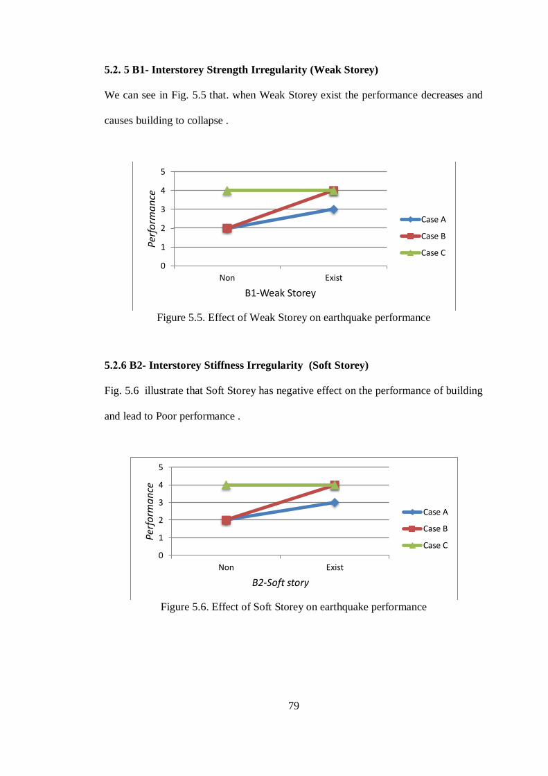
79
5.2. 5 B1- Interstorey Strength Irregularity (Weak Storey)
We can see in Fig. 5.5 that. when Weak Storey exist the performance decreases and
causes building to collapse .
Figure 5.5. Effect of Weak Storey on earthquake performance
5.2.6 B2- Interstorey Stiffness Irregularity (Soft Storey)
Fig. 5.6 illustrate that Soft Storey has negative effect on the performance of building
and lead to Poor performance .
Figure 5.6. Effect of Soft Storey on earthquake performance
0
1
2
3
4
5
Non Exist
Perf
orm
an
ce
B1-Weak Storey
Case A
Case B
Case C
0
1
2
3
4
5
Non Exist
Perf
orm
an
ce
B2-Soft story
Case A
Case B
Case C

80
5.2.7 B3 - Discontinuity of Vertical Structural Elements
The existing of B3- Discontinuity of Vertical Structural Elements lead to reduction in
the performance as Fig. 5.7 shows and collapsing may occur.
Figure 5.7. Effect of B3 - Discontinuity of Vertical Structural Elements on
earthquake performance
5.2.8 C2 Weak Column – Strong Beam
Fig. 5.8 elucidate the Effect of Weak Column – Strong Beam on earthquake
performance, this effect is very small when exist alone as in case A and also it’s
effect not significant when the effect of rest of parameters are exist as in case C but it
can be dangerous if it participated with other parameters like insufficient Stirrup
Spacing or low steel tension strength as in case B.
Figure 5.8. Effect of Weak Column – Strong Beam on earthquake performance
0
1
2
3
4
5
Non Exist
Perf
orm
an
ce
B3 - Discontinuity of Vertical Structural Elements
Case A
Case B
Case C
0
1
2
3
4
5
Non Exist
Per
form
an
ce
C2 Weak Column – Strong Beam
Case A
Case B
Case C

81
5.2.9 Stirrup Spacing
It can be noted from Fig. 5.9 that, the performance decreases when Stirrup Spacing is
not OK. If other parameters were sufficient, Stirrup Spacing has no effect or has
slight effect on the performance alone as in case A and C but this effect could be
worse in the presence of other parameters as low ratio of columns as in case B.
Figure 5.9. Effect of Stirrup Spacing on earthquake performance
5.2.10 Average Column Ratio
Fig. 5.10 shows that the Average Columns Ratio has a significant effect on the
earthquake performance especially when there is no shear walls, buildings that have
high Average Columns Ratio and do not have vertical irregularity did not collapsed
in most of the cases except when Earthquake zone (EZ) = 0.4.
Figure 5.10. Effect of Average Column Ratio on earthquake performance
0
1
2
3
4
5
OK not ok
Perf
orm
an
ce
Stirrup Spacing
Case A
Case B
Case C
0
1
2
3
4
5
0.007 0.009 0.01 0.02
Perf
orm
an
ce
Average Column Ratio
Case A
Case B
Case C

82
5.2. 11 Concrete Compression Strength (C)
According to Fig. 5.11, increasing of Concrete Compression Strength improves the
performance .
Figure 5.11. Effect of Concrete Compression Strength on earthquake
performance
5.2.12 Type of Steel
According to Fig. 5.12, increasing of Steel Tension Strength improves the
performance .
Figure 5.12. Effect of Steel Tension Strength on earthquake performance
0
1
2
3
4
5
20 25
Perf
orm
an
ce
Concrete Compression Strength
Case A
Case B
Case C
0
1
2
3
4
5
220 360
Perf
orm
an
ce
Steel Tension Strength
Case A
Case B
Case C
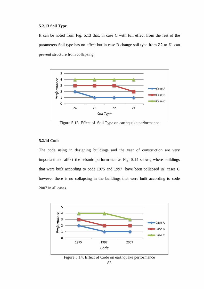
83
5.2.13 Soil Type
It can be noted from Fig. 5.13 that, in case C with full effect from the rest of the
parameters Soil type has no effect but in case B change soil type from Z2 to Z1 can
prevent structure from collapsing
Figure 5.13. Effect of Soil Type on earthquake performance
5.2.14 Code
The code using in designing buildings and the year of construction are very
important and affect the seismic performance as Fig. 5.14 shows, where buildings
that were built according to code 1975 and 1997 have been collapsed in cases C
however there is no collapsing in the buildings that were built according to code
2007 in all cases.
Figure 5.14. Effect of Code on earthquake performance
0
1
2
3
4
5
Z4 Z3 Z2 Z1
Perf
orm
an
ce
Soil Type
Case A
Case B
Case C
0
1
2
3
4
5
1975 1997 2007
Perf
orm
an
ce
Code
Case A
Case B
Case C

84
5.2.15 Earthquake zone (EZ)
Fig. 5.15 shows that, all buildings in case A still in life safety level in all the
Earthquake zones, but those in case C collapsed in zones 0.3 and 0.4 and buildings
in case B also collapsed in zones 0.4.
Figure 5.15. Effect of Earthquake Zone on earthquake performance
5.2.16 Importance Factor (I)
According to Fig. 5.16, all buildings in case C have been collapsed with all different
values of Importance Factor. On the other hand, buildings in case A and B still under
safety level except the building with Importance Factor = 1.5 in case B that enter
collapse prevention level.
Figure 5.16. Effect of Importance Factor (I) on earthquake performance
0
1
2
3
4
5
0.1 0.2 0.3 0.4
Perf
orm
an
ce
Earthquake zone (EZ)
Case A
Case B
Case C
0
1
2
3
4
5
1.0 1.2 1.4 1.5
Perf
orm
an
ce
Importance Factor (I)
Case A
Case B
Case C

85
5.3 Nonlinear Performance Analysis Model
Table 5.2. The cases used in testing of effect of each parameter Case A : The lower case Case B : The average case Case C : The upper case
(A1) = None (A1) = None (A1) = Exist
(A2) = None (A2) = None (A2) = Exist
(A3) = None (A3) = None (A3) = Exist
(B1) = None (B1) = None (B1) = Exist
(B2) = None (B2) = None (B2) = Exist
(B3) = None (B3) = None (B3) = Exist
(C2) = None (C2) = None (C2) = Exist
Stirrup Spacing = Not Ok Stirrup Spacing = Not Ok Stirrup Spacing = Ok
( ) = None ( ) = None ( ) = 0.5%
(CA) = 0.007 (CA) = 0.009 (CA) = 0.02
(C) = 20 (C) = 25 (C) = 25
(Fy) = 220 (Fy) = 360 (Fy) = 360
Soil Type = Z1 Soil Type = Z1 Soil Type = Z1
Code = 1975 Code = 1997 Code = 2007
(EZ) = 0.2 (EZ) = 0.3 (EZ) = 0.4
5.3.1 The Shear Wall Ratio
It can be noted from Fig. 5.17 that, the performance increases with increasing the
shear wall ratio while other parameters constant. This is consistent shows also that
the increasing rate in the predicted performance is larger in all cases, which means
that the shear wall ratio is the most significant structural components that affect the
performance.

86
Figure 5.17. Effect of Shear Wall Ratio on earthquake performance
5.3.2 A1-Torsional Irregularity
It can be noted from Fig. 5.18 that, the performance decreases when A1-Torsional
Irregularity be exist while other parameters constant. In other words, it is clear that
the performance is inversely proportional to the A1-Torsional Irregularity ratio .
Figure 5.18. Effect of A1-Torsional Irregularity on earthquake performance
5.3.3 A2- Slab Discontinuities
Fig. 5.19 shows that, the performance has no clear change when Slab Discontinuities
be exist while other parameters constant in case B and C and slight effect in case A.
0
1
2
3
4
5
0% 0.50% 1%
Perf
orm
an
ce
The Shear Wall Ratio
Case A
Case B
Case C
0
1
2
3
4
5
Non Exist
Perf
orm
an
ce
A1-Torsional Irregularity
Case A
Case B
Case C

87
Figure 5.19. Effect of A2- Slab Discontinuities on earthquake performance
5.3.4 A3 – Projections in Plan
Fig. 5.20 shows that the performance has no clear change when Projections in Plan
(A3) be exist while other parameters constant in case B and C and slight effect in
case A.
Figure 5.20. Effect of A3 – Projections in Plan on earthquake performance
5.3.5 B1- Interstorey Strength Irregularity (Weak Storey)
We can see in Fig. 5.21 that when Weak Storey be exist the performance decreases
and cause building collapse.
0
1
2
3
4
5
Non Exist
Perf
orm
an
ce
A2- Slab Discontinuities
Case A
Case B
Case C
0
1
2
3
4
5
Non Exist
Perf
orm
an
ce
A3 – Projections in Plan
Case A
Case B
Case C

88
Figure 5.21. Effect of Weak Storey on earthquake performance
5.3.6 B2- Interstorey Stiffness Irregularity (Soft Storey)
Fig. 5.22 illustrate that, Soft Storey has negative effect on the performance of
building and lead to Poor performance.
Figure 5.22. Effect of Soft Storey on earthquake performance
5.3.7 B3 - Discontinuity of Vertical Structural Elements
The existing of B3 - Discontinuity of Vertical Structural Elements lead to reduction
in building performance as Fig. 5.23 shows.
0
1
2
3
4
5
Non Exist
Perf
orm
an
ce
B1-Weak Storey
Case A
Case B
Case C
0
1
2
3
4
5
Non Exist
Per
form
an
ce
B2-Soft Story
Case A
Case B
Case C

89
Figure 5.23. Effect of B3 - Discontinuity of Vertical Structural Elements on
earthquake performance
5.3.8 C2 Weak Column – Strong Beam
Fig. 5.24 elucidate the effect of Weak Column–Strong Beam on earthquake
performance, this effect is very small.
Figure 5.24. Effect of Weak Column – Strong Beam on earthquake
performance
5.3.9 Stirrup Spacing
It can be noted from Fig. 5.25 that, the performance decreases when Stirrup Spacing
are be not OK. If other parameters were sufficient Stirrup Spacing has no effect in
case B and C and has slight effect on the performance in case A.
0
1
2
3
4
5
Non Exist
Perf
orm
an
ce
B3 - Discontinuity of Vertical Structural Elements
Case A
Case B
Case C
0
1
2
3
4
5
Non Exist
Per
form
an
ce
C2 Weak Column – Strong Beam
Case A
Case B
Case C

90
Figure 5.25. Effect of Stirrup Spacing on earthquake performance
5.3.10 Average Column Ratio
Fig. 5.26 shows that, the Average Columns Ratio has a significant effect on the
earthquake performance especially when there is no shear walls, buildings that have
high Average Columns Ratio and do not have vertical irregularity did not collapsed
in most of cases except when Earthquake zone (EZ) = 0.4.
Figure 5.26. Effect of Average Column Ratio on earthquake performance
5.3.11 Concrete Compression Strength (C)
According to Fig. 5.27, increasing of Concrete Compression Strength improves the
performance.
0
1
2
3
4
5
OK not ok Pe
rfo
rma
nce
Stirrup Spacing
Case A
Case B
Case C
0
1
2
3
4
5
0.007 0.009 0.01 0.02
Perf
orm
an
ce
Average Column Ratio
Case A
Case B
Case C

91
Figure 5.27. Effect of Concrete Compression Strength on earthquake
performance
5.3.12 Type of Steel
According to Fig. 5.28, increasing of Steel Tension Strength improves the
performance.
Figure 5.28. Effect of Steel Tension Strength on earthquake performance
5.3.13 Soil Type
It can be noted from Fig. 5.29 that, in analysis with nonlinear static pushover Soil
Type has more effect than the linear analysis as It can be noted from Fig. 5.29 that
changing the type of soil can be improve the performance and change the
performance collapse level (4) to collapse prevention level (3) in case C, and from
0
1
2
3
4
5
20 25
Perf
orm
an
ce
Concrete Compression Strength
Case A
Case B
Case C
0
1
2
3
4
5
220 360
Perf
orm
an
ce
Steel Tension Strength
Case A
Case B
Case C

92
collapse prevention level (3) to Life safety (2) in case B and from Life safety (2) to
Immediate Occupancy level (1) in case B.
Figure 5.29. Effect of Soil Type on earthquake performance
5.3.14 Code
The code using in designing buildings and the year of construction are very
important and Affect the Seismic Performance as Fig. 5.30 shows, where buildings
that were built according to code 1975 and 1997 have been collapsed in cases C
however there is no collapsing in the buildings that were built according to code
2007 in all cases.
Figure 5.30. Effect of Code on earthquake performance
0
1
2
3
4
5
Z4 Z3 Z2 Z1
Perf
orm
an
ce
Soil Type
Case A
Case B
Case C
0
1
2
3
4
5
1975 1997 2007
Perf
orm
an
ce
Code
Case A
Case B
Case C

93
5.3.15 Earthquake zone (EZ)
Fig. 5.31 shows that, all buildings in case A still in life safety level in all the
Earthquake zones, but those in case C collapsed in zones 0.3 and 0.4 and buildings
in case B also collapsed in zones 0.4.
Figure 5.31. Effect of Earthquake zone on earthquake performance
5.3.16 Importance Factor (I)
According to Fig. 5.32, all buildings in case C have been collapsed with all different
values of Importance Factor. On the other hand, buildings in case A and B still under
safety level except the building with Importance Factor = 1.5 in case B that enter
collapse prevention level.
Figure 5.32. Effect of Importance Factor (I) on earthquake performance
0
1
2
3
4
5
0.1 0.2 0.3 0.4
Perf
orm
an
ce
Earthquake zone (EZ)
Case A
Case B
Case C
0
1
2
3
4
5
1.0 1.2 1.4 1.5
Perf
orm
an
ce
Importance Factor (I)
Case A
Case B
Case C

94
Chapter 6
CONCLUSIONS AND RECOMMENDATIONS
6.1 Introduction
The application of Artificial Neural Networks (ANN) to evaluation the collapse
vulnerability of reinforced concrete buildings has been investigated in this Thesis.
An ANN model is built, trained and tested using the available test data of 260 RC
buildings that were modeled with the commercial program STA4cad program.
The ANN model was used to perform parametric studies in order to evaluate the
effects of the variables of on the earthquake performance which is the chosen output
parameter.
6.2 General conclusions on the use of ANN
On the basis of results obtained in this study, important conclusions would be
summarized as follows:
1) The study has added another success for Artificial Neural Networks. The ANN
are powerful tools and have strong potential in learning the relationship between the
inputs and outputs parameters and thus predicting outputs from new inputs.
2) The ANN is capable of modeling civil engineering problems.

95
6.3 Conclusions on the use of ANN in predicting earthquake
performance of RC buildings
The topology of the network for both linear and non-linear performance analysis
methods has the following features:
1- The type of architecture used was the multi-layer feed forward, three layers with
the input layer containing 16 neurons, the first hidden layer contains 10 neurons
while in the output layer there were 4 neurons. The training algorithm used was back
probation algorithm.
2- The developed neural network model in this study has succeed in predicting the
earthquake performance of RC buildings with 91% accuracy for non-linear
static pushover analysis method and about 89% accuracy for linear performance
analysis method .
6.4 Conclusions of the performed parametric study
Using the current technique the ANN, it was possible to study the effect of each of
the influencing parameters on the earthquake performance of RC buildings .
The parametric study was conducted using the trained artificial neural networks, the
following conclusions may be drawn:
6.4.1 Linear Performance Analysis model
When using the linear analysis, buildings that were built according to Code 1975 and
1997 and do not have adequate shear walls and having vertical irregularity were
collapsed in most of the cases .

96
The earthquake performance of RC buildings increases with increasing the shear wall
ratio, and has the most significant effect on the earthquake performance.
Performance decreases when A1-Torsional Irregularity exist, while other parameters
left constant. In other words, it is clear that, the performance is inversely proportional
to the A1-Torsional Irregularity ratio .
A2- Slab Discontinuities and A3 – Projections in Plan have a slight effect on the
earthquake performance when there are no shear walls and have no effect when shear
walls exist or when Average Column Ratio is high.
Moreover, the effect of stirrup spacing and strong column - weak beam is very small
when exist separately and also it’s effect not significant when the effect of rest of
parameters are exist as, but it can be dangerous if it participated together with other
parameters. Soil Type has no effect with full effect from the rest of the parameters.
However, it must be remembered that, each of these parameters have high
importance on the performance of the load-carrying system.
The Average Columns Ratio has a significant effect on the earthquake performance
especially when there is no shear walls, buildings that have high Average Columns
Ratio and do not have vertical irregularity did not collapsed in most of cases except
at Earthquake zone (EZ) = 0.4.
The predicted earthquake performance increases with the increasing of Steel Tension
Strength and Concrete Compression Strength, buildings that have Concrete

97
Compression Strength = 20 MPa or less and Steel Tension Strength =220 MPa
exposed to collapse at Earthquake zone (EZ) = 0.4 or 0.3.
6.4.2 Non-linear Performance Analysis model
When using non-linear analysis method, to evaluate the earthquake performance of
RC buildings the numbers of buildings that collapsed is less than linear analysis
method especially for the structures that have irregularites and Soil Type has more
effect than the linear analysis.
6.5 Recommendations for future studies
The current study showed very promising results in predicting the earthquake
performance of RC buildings. However, the following points would be
recommended for future studies to support the findings of this study:
1- It is recommended to carry out neural network modeling using different ANN
types such as recurrent networks with various training algorithms such as radial
bases can be used.
2- It is recommended to utilize other artificial intelligence techniques such as fuzzy
logic or genetic programming to compare their results.
3- Obtain more training data from newly tested buildings models and add them to the
training data. This will improve the training process of the problem.

98
REFERENCES
[1] Dutykh, D., & Dias, F. (2010). Influence of sedimentary layering on tsunami
generation. Computer Methods in Applied Mechanics and Engineering,199(21),
1268-1275.
[2] Bal, I. E. (2005). Rapid assessment techniques for collapse vulnerability of
reinforced concrete buildings (Doctoral dissertation, MSc Thesis, İstanbul
Technical University, Civil Engineering Department (in Turkish)).
[3] Ohkubo, M. (1990). The method for evaluating seismic performance of existing
reinforced concrete buildings. In Seminar in Structural Engineering, Dept. of
AMES, University of California, San Diego.
[4] Boduroglu, H., Ozdemir, P., Ilki, A., Sirin, S., Demir, C., & Baysan, F. (2004,
August). Towards a modified rapid screening method for existing medium rise
RC buildings in Turkey. In 13th World Conference on Earthquake
Engineering (Vol. 13, pp. 1-6).
[5] Hassan, A. F., & Sozen, M. A. (1997). Seismic vulnerability assessment of low-
rise buildings in regions with infrequent earthquakes. ACI Structural
Journal, 94(1), 31-39.
[6] FEMA, 2015, Rapid Visual Screening of Buildings for Potential Seismic
Hazards: A Handbook, Third Edition, FEMA P-154, prepared by the Applied

99
Technology Council for the Federal Emergency Management Agency,
Washington, D.C.
[7] Arslan, M. H. (2010). An evaluation of effective design parameters on earthquake
performance of RC buildings using neural networks. Engineering
Structures, 32(7), 1888-1898.
[8] Arslan, M. H., Ceylan, M., & Koyuncu, T. (2015). Determining earthquake
performances of existing reinforced concrete buildings by using ANN. World
Acad Sci Eng Technol Int J Civ Environ Struct Constr Archit Eng, 9(8), 921-925.
[9] TEC-2007, Turkish Earthquake Code. Regulations on structures constructed in
disaster regions. Ministry of Public Works and Settlement Ankara. 2007 (In
Turkish).
[11] Al-Najjar, H., 2005. Prediction of Ultimate Shear Strength of Reinforced
Concrete Deep Beams Using Artificial Neural Networks, Gaza strip. Master
Thesis in construction management, The Islamic University of Gaza Strip.
[11] Neural Network Toolbox User's Guide . 2015.
[12] Shahin, M. A., Jaksa, M. B., & Maier, H. R. (2001). Artificial neural network
applications in geotechnical engineering. Australian Geomechanics, 36(1), 49-62.
[13] Ashour, A.F & Alqedra, M.A. (2004) “Concrete Breakout Strenght of Single
Anchors in Tension using Neural Networks ". Engineering Software-Elsevier .

100
[14] Kirkegaard, P. H. & Rytter A. )1993(. “Use of Neural Networks for Damage
Detection and Location in a Steel Member ". Proc. of the 3rd International
Conference on the Application of Artificial Intelligence to Civil and Structural
Engineering. CIVILCOMP93, Edinburgh, August 17-19.
[15] Shahin, M.A, Maier, H.R, JAKSA, M.B (2002) “Predicting Settlement of
Shallow Foundations Using Neural Networks". Journal of Geotechnical and
Geoenvironmental Engineering .
[10] Ni, H. G., & Wang, J. Z. (2000). Prediction of compressive strength of concrete
by neural networks. Cement and Concrete Research, 30(8), 1245-1250.
[10] Neural networks http://www.cse.unsw.edu.au/~billw/mldict.html[2012].
[18] Rafiq, M. Y., Bugmann, G., & Easterbrook, D. J. (2001). Neural network
design for engineering applications. Computers & Structures, 79(17), 1541-1552.
[19] OBrien, E. J., & Dixon, A. S. (1995). Reinforced and prestressed concrete
design: the complete process. Longman Scientific & Technical; Copublished in
the United States with J. Wiley.
[21] Neural networks http://scom.hud.ac.uk/scomtlm/book/node358.html[2012].
[21] Haykin, S.(1999) 2nd ed. Neural Networks A comprehensive Fundamentals.
Prentice-Hall ,Inc: New Jersey.
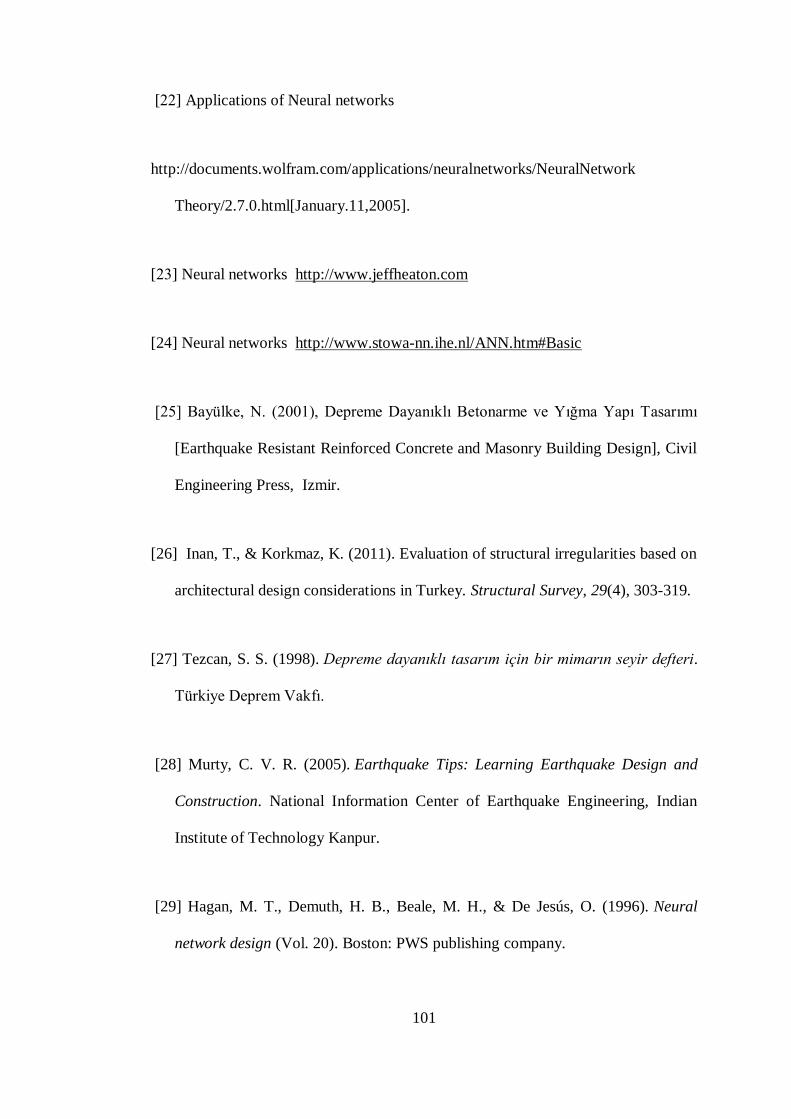
101
[22] Applications of Neural networks
http://documents.wolfram.com/applications/neuralnetworks/NeuralNetwork
Theory/2.7.0.html[January.11,2005].
[23] Neural networks http://www.jeffheaton.com
[24] Neural networks http://www.stowa-nn.ihe.nl/ANN.htm#Basic
[25] Bayülke, N. (2001), Depreme Dayanıklı Betonarme ve Yığma Yapı Tasarımı
[Earthquake Resistant Reinforced Concrete and Masonry Building Design], Civil
Engineering Press, Izmir.
[26] Inan, T., & Korkmaz, K. (2011). Evaluation of structural irregularities based on
architectural design considerations in Turkey. Structural Survey, 29(4), 303-319.
[27] Tezcan, S. S. (1998). Depreme dayanıklı tasarım için bir mimarın seyir defteri.
Türkiye Deprem Vakfı.
[28] Murty, C. V. R. (2005). Earthquake Tips: Learning Earthquake Design and
Construction. National Information Center of Earthquake Engineering, Indian
Institute of Technology Kanpur.
[29] Hagan, M. T., Demuth, H. B., Beale, M. H., & De Jesús, O. (1996). Neural
network design (Vol. 20). Boston: PWS publishing company.

102
[30] Mansour, M. Y., Dicleli, M., Lee, J. Y., & Zhang, J. (2004). Predicting the
shear strength of reinforced concrete beams using artificial neural
networks.Engineering Structures, 26(6), 781-799.
[31] MathWorks Inc. MatLab the language of technical computing. Natick, MA,
USA: MathWorks Inc; )1999(. Version 6.5.
[32] High performance concrete
http://www.jeffheaton.com/ai/javaneural/ch5.shtml[January.11,2005].
[33] Jamous, E. H. A. (2013). M. Sc. Thesis Parametric Cost Estimation of Road
Projects Using Artificial Neural Networks (Doctoral dissertation, The Islamic
University–Gaza).
[34] Oreta, A. W. C. (2004). Simulating size effect on shear strength of RC beams
without stirrups using neural networks. Engineering Structures, 26(5), 681-691.
[35] Ilki, A., & Celep, Z. (2012). Earthquakes, existing buildings and seismic design
codes in Turkey. Arabian Journal for Science and Engineering, 37(2), 365-380.

103
APPENDIX

104
Appendix A: Data Used in The Study
10
0
0
0
0
0
0
0
1
0
0.00
96
25
220
Z1
2007
0.3
1 2
2
9
0
0
0
0
0
0
0
1
0
0.00
96
25
220
Z1
2007
0.3
1
2
2
8
0
0
0
0
0
0
0
1
0
0.00
96
20
220
Z1
2007
0.3
1
2 2
0 0 0 0 0 0 0 0 1 0
0.00
96
20
220
Z1
1975
0.4
1
2
3
6
0
0
0
0
0
0
0
1
0
0.00
96
20
220
Z1
1975
0.4
1
4 4
1 0 0 0 0 0 0 0 1 0
0.00
96
25
220
Z1
1997
0.4
1
2
2
4 0 0 0 0 0 0 0 1 0
0.00
96
20
220
Z1
1997
0.4
1
3 2
3 0 0 0 0 0 0 0 1 0
0.00
96
20
220
Z1
1997
0.4
1
3 4
2 0 0 0 0 0 0 0 1 0
0.00
96
25
220
Z1
2007
0.4
1
2 2
1 0 0 0 0 0 0 0 1 0
0.0
096
25
220
Z1
2007
0.4
1
2 2
Par
am
eter
A1-
Tors
ion
al Ir
regu
lari
ty
A2-
Sla
b D
isco
nti
nu
itie
s
A3 –
Pro
ject
ion
s in
Pla
n
B1
- In
ters
tore
y St
ren
gth
Irre
gula
rity
(W
eak
Sto
rey)
B2-
Inte
rsto
rey
Stif
fnes
s Ir
regu
lari
ty (
Soft
St
ore
y)
B3
- D
isco
nti
nui
ty o
f V
erti
cal S
tru
ctu
ral
Elem
ents
C2
Wea
k C
olu
mn
– S
tro
ng
Bea
m
Stir
rup
Sp
acin
g
Ave
rage
Sh
ear
Wal
l Rat
io (
)
Ave
rage
Co
lum
n R
atio
(
CA
)
Co
ncr
ete
Co
mp
ress
ion
Stre
ngt
h (C
)
Typ
e o
f st
eel
Soil
Type
(Z)
Co
de
Eart
hqu
ake
zon
e (E
Z)
Imp
orta
nce
Fac
tor
(I)
Stru
ctu
ral P
erfo
rman
ce (
S1-S
4) L
inea
r /n
on
lin
ear

105
Parameter 11 12 13 14 15 16 17 18 19 20
A1-Torsional Irregularity 0 0 0 0 0 0 0 0 0 0
A2- Slab Discontinuities 0 0 0 0 0 0 0 0 0 0
A3 – Projections in Plan 0 0 0 0 0 0 0 0 0 0
B1- Interstorey Strength Irregularity (Weak Storey).
0 0 0 0 0 0 0 0 0 0
B2- Interstorey Stiffness Irregularity (Soft Storey)
0 0 0 0 0 0 0 0 0 0
B3 - Discontinuity of Vertical Structural Elements
0 0 0 0 0 0 0 0 0 0
C2 Weak Column – Strong Beam 0 0 0 0 0 0 0 0 0 0
Stirrup Spacing 1 1 1 1 1 1 1 1 1 1
Average Shear Wall Ratio ( ) 0 0 0 0 0 0 0 0 0 0
Average Column Ratio ( CA) 0.0096 0.0096 0.0096 0.0096 0.0096 0.0096 0.0096 0.0096 0.0096 0.0096
Concrete Compression Strength (C) 20 25 25 20 20 25 25 20 20 25
Type of steel 360 220 360 220 360 220 360 220 360 220
Soil Type (Z) Z1 Z1 Z1 Z1 Z1 Z1 Z1 Z1 Z1 Z1
Code 1997 1997 1997 1975 1975 1975 2007 1997 1997 1997
Earthquake zone (EZ) 0.3 0.3 0.3 0.3 0.3 0.3 0.2 0.2 0.2 0.2
Importance Factor (I) 1 1 1 1 1 1 1 1 1 1
Structural Performance (S1-S4) 2 2 2 2 2 2 4 2 2 2 4 2 1 1 1 1 1 1 1 1

106
Parameter 21 22 23 24 25 26 27 28 29 30
A1-Torsional Irregularity 0 0 0 0 0 0 0 0 0 0
A2- Slab Discontinuities 0 0 0 0 0 0 0 0 0 0
A3 – Projections in Plan 0 0 0 0 0 0 0 0 0 0
B1- Interstorey Strength Irregularity (Weak Storey).
0 0 0 0 0 0 0 0 1 1
B2- Interstorey Stiffness Irregularity (Soft Storey)
0 0 0 0 0 0 0 0 1 1
B3 - Discontinuity of Vertical Structural Elements
0 0 0 0 0 0 0 0 0 0
C2 Weak Column – Strong Beam 0 0 0 0 0 0 0 0 0 0
Stirrup Spacing 1 1 1 1 1 1 1 1 1 1
Average Shear Wall Ratio ( ) 0 0 0 0 0 0 0 0 0 0
Average Column Ratio ( CA) 0.0096 0.0096 0.0096 0.0096 0.0096 0.0096 0.0096 0.0096 0.01 0.01
Concrete Compression Strength (C) 20 20 25 20 20 25 20 20 25 20
Type of steel 220 360 360 220 360 360 220 360 360 360
Soil Type (Z) Z1 Z2 Z1 Z1 Z1 Z1 Z2 Z1 Z2 Z1
Code 1975 1975 2007 1997 1997 1997 1975 1975 2007 1997
Earthquake zone (EZ) 0.2 0.2 0.1 0.1 0.1 0.1 0.1 0.1 0.4 0.4
Importance Factor (I) 1 1 1 1 1 1 1 1 1 1
Structural Performance (S1-S4) 3 2 2 2 1 1 1 1 1 1 1 1 2 1 1 1 2 2 3 2

107
Parameter 31 32 33 34 35 36 37 38 39 40
A1-Torsional Irregularity 0 0 0 0 0 0 0 0 0 0
A2- Slab Discontinuities 0 0 0 0 0 0 0 0 0 0
A3 – Projections in Plan 0 0 0 0 0 0 0 0 0 0
B1- Interstorey Strength Irregularity (Weak Storey).
1 1 1 1 1 1 1 0 0 0
B2- Interstorey Stiffness Irregularity (Soft Storey)
1 1 1 1 1 1 1 0 0 0
B3 - Discontinuity of Vertical Structural Elements
0 0 0 0 0 0 0 1 1 1
C2 Weak Column – Strong Beam 0 0 0 0 0 0 0 0 0 0
Stirrup Spacing 1 1 1 1 1 1 1 1 1 1
Average Shear Wall Ratio ( ) 0 0 0 0 0 0 0 0 0 0
Average Column Ratio ( CA) 0.01 0.01 0.01 0.01 0.01 0.01 0.01 0.01 0.01 0.01
Concrete Compression Strength (C) 20 25 25 20 20 20 20 25 20 20
Type of steel 220 360 360 360 220 360 220 360 360 220
Soil Type (Z) Z1 Z2 Z2 Z3 Z3 Z4 Z2 Z1 Z1 Z1
Code 1975 1975 2007 1997 1975 1975 1975 2007 1997 1975
Earthquake zone (EZ) 0.4 0.4 0.3 0.2 0.2 0.2 0.1 0.4 0.4 0.4
Importance Factor (I) 1 1 1 1 1 1 1 1 1 1
Structural Performance (S1-S4) 4 4 3 3 2 2 1 1 3 2 2 2 2 1 3 2 3 2 4 2

108
Parameter 41 42 43 44 45 46 47 48 49 50
A1-Torsional Irregularity 0 0 0 0 0 0 0 0 0 0
A2- Slab Discontinuities 0 0 0 0 0 0 0 0 0 0
A3 – Projections in Plan 0 0 0 0 0 0 0 0 0 0
B1- Interstorey Strength Irregularity (Weak Storey).
0 0 0 0 0 0 0 0 1 1
B2- Interstorey Stiffness Irregularity (Soft Storey)
0 0 0 0 0 0 0 0 1 1
B3 - Discontinuity of Vertical Structural Elements
1 1 1 1 1 1 0 0 0 0
C2 Weak Column – Strong Beam 0 0 0 0 0 0 0 0 0 0
Stirrup Spacing 1 1 1 1 1 1 0 0 0 0
Average Shear Wall Ratio ( ) 0 0 0 0 0 0 0 0 0 0
Average Column Ratio ( CA) 0.0096 0.0096 0.0096 0.0096 0.0097 0.0096 0.0096 0.0094 0.0094 0.01
Concrete Compression Strength (C) 20 25 20 20 20 20 25 20 20 20
Type of steel 360 360 360 220 360 220 360 360 220 360
Soil Type (Z) Z1 Z1 Z1 Z1 Z1 Z1 Z1 Z1 Z1 Z1
Code 1975 2007 1997 1975 1975 1975 2007 1997 1975 1975
Earthquake zone (EZ) 0.4 0.3 0.2 0.2 0.2 0.1 0.4 0.4 0.4 0.4
Importance Factor (I) 1 1 1 1 1 1 1 1 1 1
Structural Performance (S1-S4) 4 3 3 2 3 1 3 1 3 1 3 1 4 2 4 2 4 4 3 2

109
Parameter 51 52 53 54 55 56 57 58 59 60
A1-Torsional Irregularity 0 0 0 0 0 0 0 0 0 0
A2- Slab Discontinuities 0 0 0 0 0 0 0 0 0 0
A3 – Projections in Plan 0 0 0 0 0 0 0 0 0 0
B1- Interstorey Strength Irregularity (Weak Storey).
0 0 1 1 1 0 0 0 0 0
B2- Interstorey Stiffness Irregularity (Soft Storey)
0 0 1 1 1 0 0 0 0 0
B3 - Discontinuity of Vertical Structural Elements
0 0 0 0 0 0 0 0 0 0
C2 Weak Column – Strong Beam 0 0 0 0 0 1 1 1 1 1
Stirrup Spacing 0 0 0 0 0 0 0 0 0 0
Average Shear Wall Ratio ( ) 0 0 0 0 0 0 0 0 0 0
Average Column Ratio ( CA) 0.0093 0.0099 0.0096 0.0096 0.0096 0.0096 0.0096 0.0096 0.0098 0.0098
Concrete Compression Strength (C) 25 20 20 20 20 25 20 20 20 25
Type of steel 360 360 220 360 220 360 360 220 360 360
Soil Type (Z) Z1 Z1 Z1 Z1 Z1 Z1 Z1 Z1 Z1 Z1
Code 2007 1997 1975 1975 1975 2007 1997 1975 1975 2007
Earthquake zone (EZ) 0.3 0.2 0.2 0.2 0.1 0.4 0.4 0.4 0.4 0.3
Importance Factor (I) 1 1 1 1 1 1 1 1 1 1
Structural Performance (S1-S4) 4 2 2 2 2 1 2 1 2 1 2 2 2 2 3 4 2 4 2 2

110
Parameter 61 62 63 64 65 66 67 68 69 70
A1-Torsional Irregularity 0 0 0 0 0 0 0 0 0 0
A2- Slab Discontinuities 0 0 0 0 Case 1 Case 1 Case 1 Case 1 Case 1 Case 1
A3 – Projections in Plan 0 0 0 0 1 1 1 1 1 1
B1- Interstorey Strength Irregularity (Weak Storey).
0 0 0 0 1 1 1 1 1 1
B2- Interstorey Stiffness Irregularity (Soft Storey)
0 0 0 0 1 1 1 1 1 1
B3 - Discontinuity of Vertical Structural Elements
0 0 0 0 1 1 1 1 1 1
C2 Weak Column – Strong Beam 1 1 1 1 1 1 1 1 1 1
Stirrup Spacing 0 0 0 0 0 0 0 0 0 0
Average Shear Wall Ratio ( ) 0 0 0 0 0 0 0 0 0 0
Average Column Ratio ( CA) 0.0096 0.0096 0.0096 0.0096 0.0096 0.0096 0.0096 0.0096 0.0096 0.0096
Concrete Compression Strength (C) 20 20 20 20 25 20 20 20 25 20
Type of steel 360 220 360 220 360 360 220 360 360 360
Soil Type (Z) Z1 Z1 Z1 Z1 Z1 Z1 Z1 Z1 Z1 Z1
Code 1997 1975 1975 1975 2007 1997 1975 1975 2007 1997
Earthquake zone (EZ) 0.2 0.2 0.2 0.1 0.4 0.4 0.4 0.4 0.3 0.2
Importance Factor (I) 1 1 1 1 1 1 1 1 1 1
Structural Performance (S1-S4) 2 2 2 2 2 2 2 1 4 3 4 3 4 3 4 3 4 3 4 3

111
Parameter 71 72 73 74 75 76 77 78 79 80
A1-Torsional Irregularity 0 0 0 1 1 1 1 1 1 1
A2- Slab Discontinuities Case 1 Case 1 Case 1 0 0 0 0 0 0 0
A3 – Projections in Plan 1 1 1 0 0 0 0 0 0 0
B1- Interstorey Strength Irregularity (Weak Storey).
1 1 1 0 0 0 0 0 0 0
B2- Interstorey Stiffness Irregularity (Soft Storey)
1 1 1 0 0 0 0 0 0 0
B3 - Discontinuity of Vertical Structural Elements
1 1 1 0 0 0 0 0 0 0
C2 Weak Column – Strong Beam 1 1 1 0 0 0 0 0 0 0
Stirrup Spacing 0 0 0 1 1 1 1 1 1 1
Average Shear Wall Ratio ( ) 0 0 0 0 0 0 0 0 0 0
Average Column Ratio ( CA) 0.01 0.01 0.01 0.01 0.01 0.01 0.01 0.01 0.01 0.01
Concrete Compression Strength (C) 20 20 20 25 20 20 20 25 20 20
Type of steel 220 360 220 360 360 220 360 360 360 220
Soil Type (Z) Z3 Z3 Z2 Z2 Z2 Z4 Z4 Z2 Z2 Z2
Code 1975 1975 1975 2007 1997 1975 1975 2007 1997 1975
Earthquake zone (EZ) 0.2 0.2 0.1 0.4 0.4 0.4 0.4 0.3 0.2 0.2
Importance Factor (I) 1 1 1 1 1 1 1 1 1 1
Structural Performance (S1-S4) 4 3 4 3 3 1 2 2 2 2 4 3 4 3 2 2 2 2 3 2

112
Parameter 81 82 83 84 85 86 87 88 89 90
A1-Torsional Irregularity 1 1 1 1 1 1 1 1 1 1
A2- Slab Discontinuities 0 0 0 0 0 0 0 0 0 0
A3 – Projections in Plan 0 0 0 0 0 0 0 0 0 0
B1- Interstorey Strength Irregularity (Weak Storey).
0 0 0 0 0 0 0 0 0 0
B2- Interstorey Stiffness Irregularity (Soft Storey)
0 0 0 0 0 0 0 0 0 0
B3 - Discontinuity of Vertical Structural Elements
0 0 0 0 0 0 0 0 0 0
C2 Weak Column – Strong Beam 0 0 0 0 0 0 0 0 0 0
Stirrup Spacing 1 1 0 0 0 0 0 0 0 0
Average Shear Wall Ratio ( ) 0 0 0 0 0 0 0 0 0 0
Average Column Ratio ( CA) 0.01 0.01 0.01 0.01 0.01 0.01 0.01 0.01 0.01 0.01
Concrete Compression Strength (C) 20 20 25 20 20 20 25 20 20 20
Type of steel 360 220 360 360 220 360 360 360 220 360
Soil Type (Z) Z1 Z1 Z1 Z1 Z1 Z1 Z1 Z1 Z1 Z1
Code 1975 1975 2007 1997 1975 1975 2007 1997 1975 1975
Earthquake zone (EZ) 0.2 0.1 0.4 0.4 0.4 0.4 0.3 0.2 0.2 0.2
Importance Factor (I) 1 1 1 1 1 1 1 1 1 1
Structural Performance (S1-S4) 3 2 2 2 2 2 2 2 3 3 3 2 2 2 2 2 2 2 2 2

113
Parameter 91 92 93 94 95 96 97 98 99 100
A1-Torsional Irregularity 1 1 1 1 1 1 1 1 1 1
A2- Slab Discontinuities 0 0 0 0 0 0 0 0 0 0
A3 – Projections in Plan 0 0 0 0 0 0 0 0 0 0
B1- Interstorey Strength Irregularity (Weak Storey).
0 1 1 1 1 1 1 1 1 1
B2- Interstorey Stiffness Irregularity (Soft Storey)
0 1 1 1 1 1 1 1 1 1
B3 - Discontinuity of Vertical Structural Elements
0 1 1 1 1 1 1 1 1 1
C2 Weak Column – Strong Beam 0 1 1 1 1 1 1 1 1 1
Stirrup Spacing 0 0 0 0 0 0 0 0 0 0
Average Shear Wall Ratio ( ) 0 0 0 0 0 0 0 0 0 0
Average Column Ratio ( CA) 0.01 0.01 0.01 0.01 0.01 0.01 0.01 0.01 0.01 0.01
Concrete Compression Strength (C) 20 25 20 20 20 25 20 20 20 20
Type of steel 220 360 360 220 360 360 360 220 360 220
Soil Type (Z) Z1 Z2 Z2 Z1 Z1 Z2 Z1 Z1 Z1 Z1
Code 1975 2007 1997 1975 1975 2007 1997 1975 1975 1975
Earthquake zone (EZ) 0.1 0.4 0.4 0.4 0.4 0.3 0.2 0.2 0.2 0.1
Importance Factor (I) 1 1 1 1 1 1 1 1 1 1
Structural Performance (S1-S4) 2 1 4 3 4 3 4 3 4 3 4 3 4 3 4 3 4 3 3 1

114
Parameter 101 102 103 104 105 106 107 108 109 110
A1-Torsional Irregularity 0 0 0 0 0 0 0 0 0 0
A2- Slab Discontinuities 0 0 0 0 0 0 0 0 0 0
A3 – Projections in Plan 0 0 0 0 0 0 0 0 0 0
B1- Interstorey Strength Irregularity (Weak Storey).
0 0 0 0 0 0 0 0 0 0
B2- Interstorey Stiffness Irregularity (Soft Storey)
0 0 0 0 0 0 0 0 0 0
B3 - Discontinuity of Vertical Structural Elements
0 0 0 0 0 0 0 0 0 0
C2 Weak Column – Strong Beam 0 0 0 0 0 0 0 0 0 0
Stirrup Spacing 1 1 1 1 1 1 1 1 1 1
Average Shear Wall Ratio ( ) 0.008 0.003 0.003 0.005 0.008 0.008 0.003 0.007 0.0025 0.0045
Average Column Ratio ( CA) 0.0096 0.01 0.01 0.0096 0.0096 0.0096 0.0096 0.0096 0.0096 0.0096
Concrete Compression Strength (C) 25 20 20 25 20 20 25 20 25 25
Type of steel 360 220 360 360 220 360 360 360 220 360
Soil Type (Z) Z1 Z1 Z1 Z1 Z1 Z1 Z1 Z1 Z1 Z1
Code 2007 1997 1997 1997 1975 1975 2007 1997 1997 1997
Earthquake zone (EZ) 0.4 0.4 0.4 0.4 0.4 0.4 0.3 0.3 0.3 0.3
Importance Factor (I) 1 1 1 1 1 1 1 1 1 1
Structural Performance (S1-S4) 2 2 3 2 3 2 2 1 3 1 2 1 2 2 2 1 2 2 2 1

115
Parameter 111 112 113 114 115 116 117 118 119 120
A1-Torsional Irregularity 0 0 0 0 0 1 1 1 1 1
A2- Slab Discontinuities 0 0 0 0 0 0 0 0 0 0
A3 – Projections in Plan 0 0 0 0 0 0 0 0 0 0
B1- Interstorey Strength Irregularity (Weak Storey).
0 0 0 0 0 1 1 1 1 1
B2- Interstorey Stiffness Irregularity (Soft Storey)
0 0 0 0 0 1 1 1 1 1
B3 - Discontinuity of Vertical Structural Elements
0 0 0 0 0 1 1 1 1 1
C2 Weak Column – Strong Beam 0 0 0 0 0 1 1 1 1 1
Stirrup Spacing 1 1 1 1 1 0 0 0 0 0
Average Shear Wall Ratio ( ) 0.0055 0.003 0.0075 0.0075 0.0025 0.005 0.0045 0.008 0.005 0.0045
Average Column Ratio ( CA) 0.01 0.01 0.01 0.01 0.01 0.01 0.01 0.01 0.01 0.01
Concrete Compression Strength (C) 20 20 25 20 20 25 20 20 25 20
Type of steel 220 360 220 220 220 360 220 360 360 220
Soil Type (Z) Z3 Z3 Z4 Z4 Z2 Z1 Z1 Z1 Z1 Z1
Code 1975 1975 1975 1975 1975 2007 1997 1997 1997 1975
Earthquake zone (EZ) 0.3 0.3 0.3 0.2 0.1 0.4 0.4 0.4 0.4 0.4
Importance Factor (I) 1 1 1 1 1 1 1 1 1 1
Structural Performance (S1-S4) 2 1 2 2 2 1 1 1 1 1 4 2 4 3 3 3 4 3 4 3

116
Parameter 121 122 123 124 125 126 127 128 129 130
A1-Torsional Irregularity 1 1 1 1 1 1 1 1 1 1
A2- Slab Discontinuities 0 0 0 0 0 0 0 0 0 0
A3 – Projections in Plan 0 0 0 0 0 0 0 0 0 0
B1- Interstorey Strength Irregularity (Weak Storey).
1 1 1 1 1 1 1 1 1 1
B2- Interstorey Stiffness Irregularity (Soft Storey)
1 1 1 1 1 1 1 1 1 1
B3 - Discontinuity of Vertical Structural Elements
1 1 1 1 1 1 1 1 1 1
C2 Weak Column – Strong Beam 1 1 1 1 1 1 1 1 1 1
Stirrup Spacing 0 0 0 0 0 0 0 0 0 0
Average Shear Wall Ratio ( ) 0.0085 0.05 0.007 0.0045 0.002 0.007 0.003 0.008 0.0055 .0045
Average Column Ratio ( CA) 0.01 0.01 0.01 0.01 0.01 0.01 0.01 0.01 0.01 0.01
Concrete Compression Strength (C) 20 25 20 25 25 20 20 25 25 20
Type of steel 360 360 360 220 360 220 360 220 360 360
Soil Type (Z) Z1 Z1 Z1 Z1 Z1 Z1 Z1 Z1 Z1 Z1
Code 1975 2007 1997 1997 1997 1975 1975 1975 2007 1997
Earthquake zone (EZ) 0.4 0.3 0.3 0.3 0.3 0.3 0.3 0.3 0.2 0.2
Importance Factor (I) 1 1 1 1 1 1 1 1 1 1
Structural Performance (S1-S4) 4 3 4 2 4 3 4 3 4 3 4 3 4 3 4 3 4 2 4 3
117
Parameter 131 132 133 134 135 136 137 138 139 140
A1-Torsional Irregularity 1 1 1 1 1 1 1 1 0 0
A2- Slab Discontinuities 0 0 0 0 0 0 0 0 0 0
A3 – Projections in Plan 0 0 0 0 0 0 0 0 0 0
B1- Interstorey Strength Irregularity (Weak Storey).
1 1 1 1 1 1 1 1 0 0
B2- Interstorey Stiffness Irregularity (Soft Storey)
1 1 1 1 1 1 1 1 0 0
B3 - Discontinuity of Vertical Structural Elements
1 1 1 1 1 1 1 1 0 0
C2 Weak Column – Strong Beam 1 1 1 1 1 1 1 1 0 0
Stirrup Spacing 0 0 0 0 0 0 0 0 1 1
Average Shear Wall Ratio ( ) 0.0085 0.005 0.004 0.008 0.005 0.004 0.003 0.003 0 0
Average Column Ratio ( CA) 0.01 0.01 0.01 0.01 0.01 0.01 0.01 0.01 0.0095 0.0072
Concrete Compression Strength (C) 20 20 25 20 20 25 20 20 25 20
Type of steel 220 360 360 220 360 360 220 360 360 360
Soil Type (Z) Z3 Z3 Z4 Z4 Z1 Z1 Z1 Z1 Z2 Z1
Code 1975 1975 2007 1997 1997 1997 1975 1975 2007 1997
Earthquake zone (EZ) 0.2 0.2 0.1 0.1 0.1 0.1 0.1 0.1 0.4 0.4
Importance Factor (I) 1 1 1 1 1 1 1 1 1 1
Structural Performance (S1-S4) 4 3 4 3 3 2 4 3 3 2 3 2 4 3 4 2 2 2 4 2

118
Parameter 141 142 143 144 141 146 140 148 149 110
A1-Torsional Irregularity 0 0 0 0 0 0 0 0 0 0
A2- Slab Discontinuities 0 0 0 0 0 0 0 0 0 0
A3 – Projections in Plan 0 0 0 0 0 0 0 0 0 0
B1- Interstorey Strength Irregularity (Weak Storey).
0 0 0 0 0 0 0 0 0 0
B2- Interstorey Stiffness Irregularity (Soft Storey)
0 0 0 0 0 0 0 0 0 0
B3 - Discontinuity of Vertical Structural Elements
0 0 0 0 0 0 0 0 0 0
C2 Weak Column – Strong Beam 0 0 0 0 0 0 0 0 0 0
Stirrup Spacing 1 1 1 1 1 1 1 1 1 1
Average Shear Wall Ratio ( ) 0 0 0 0 0 0 0 0 0 0
Average Column Ratio ( CA) 0.0084 0.009 0.013 0.009 0.012 0.0087 0.0087 0.0082 0.0095 0.0058
Concrete Compression Strength (C) 20 20 25 25 20 25 25 25 25 25
Type of steel 220 360 220 360 220 360 220 220 220 220
Soil Type (Z) Z1 Z1 Z1 Z1 Z2 Z2 Z2 Z2 Z1 Z1
Code 1975 1975 1997 1997 1975 1975 1975 1997 1997 1975
Earthquake zone (EZ) 0.4 0.4 0.3 0.3 0.3 0.3 0.3 0.3 0.3 0.2
Importance Factor (I) 1 1 1 1 1 1 1 1 1 1
Structural Performance (S1-S4) 4 3 3 2 3 2 2 2 4 3 3 2 4 3 3 2 2 2 2 2

119
Parameter 111 112 113 114 111 116 110 118 119 160
A1-Torsional Irregularity 1 1 1 1 1 1 1 1 1 1
A2- Slab Discontinuities 0 0 0 0 0 0 0 0 0 0
A3 – Projections in Plan 0 0 0 0 0 0 0 0 0 0
B1- Interstorey Strength Irregularity (Weak Storey).
1 1 1 1 1 1 1 1 1 1
B2- Interstorey Stiffness Irregularity (Soft Storey)
1 1 1 1 1 1 1 1 1 1
B3 - Discontinuity of Vertical Structural Elements
1 1 1 1 1 1 1 1 1 1
C2 Weak Column – Strong Beam 1 1 1 1 1 1 1 1 1 1
Stirrup Spacing 0 0 0 0 0 0 0 0 0 0
Average Shear Wall Ratio ( ) 0 0 0 0 0 0 0 0 0 0
Average Column Ratio ( CA) 0.019 0.019 0.02 0.017 0.018 0.018 0.015 0.016 0.015 0.016
Concrete Compression Strength (C) 25 20 20 20 25 25 20 20 20 20
Type of steel 360 360 220 360 360 360 360 220 360 220
Soil Type (Z) Z1 Z1 Z1 Z1 Z2 Z2 Z2 Z2 Z1 Z1
Code 2007 1997 1975 1975 1997 2007 1997 1975 1975 1975
Earthquake zone (EZ) 0.4 0.4 0.4 0.4 0.3 0.3 0.2 0.2 0.2 0.1
Importance Factor (I) 1 1 1 1 1 1 1 1 1 1
Structural Performance (S1-S4) 4 3 4 4 4 4 4 3 3 2 3 2 4 2 4 3 3 2 4 3

120
Parameter 161 162 163 164 165 166 167 168 169 100
A1-Torsional Irregularity 0 0 0 0 0 0 0 0 0 0
A2- Slab Discontinuities 0 0 0 0 0 0 0 0 0 0
A3 – Projections in Plan 0 0 0 0 0 0 0 0 0 0
B1- Interstorey Strength Irregularity (Weak Storey).
0 0 0 0 0 0 0 0 0 0
B2- Interstorey Stiffness Irregularity (Soft Storey)
0 0 0 0 0 0 0 0 0 0
B3 - Discontinuity of Vertical Structural Elements
0 0 0 0 0 0 0 0 0 0
C2 Weak Column – Strong Beam 0 0 0 0 0 0 0 0 0 0
Stirrup Spacing 1 1 1 1 1 1 1 1 1 1
Average Shear Wall Ratio ( ) 0 0 0 0 0 0 ,L 0 0 0 0
Average Column Ratio ( CA) [40*40]*30/500 0.0096 0.0096 0.0096 0.0096 0.0096 0.0096 0.0096 0.0096 0.0096
Concrete Compression Strength (C) 25 25 20 20 25 20 20 20 25 25
Type of steel 220 360 220 360 360 220 360 360 220 360
Soil Type (Z) Z2 Z2 Z2 Z2 Z2 Z2 Z2 Z2 Z2 Z2
Code 2007 2007 1997 1997 1997 1975 1975 2007 2007 2007
Earthquake zone (EZ) 0.4 0.4 0.4 0.4 0.4 0.4 0.4 0.3 0.3 0.3
Importance Factor (I) 1 1 1 1 1 1 1 1 1 1
Structural Performance (S1-S4) Lin /non lin 2 2 2 2 4 3 2 3 2 2 4 4 4 2 2 2 2 2 2 2

121
Parameter 101 102 103 104 105 106 107 108 109 180
A1-Torsional Irregularity 0 0 0 0 0 0 0 0 0 0
A2- Slab Discontinuities 0 0 0 0 0 0 0 0 0 0
A3 – Projections in Plan 0 0 0 0 0 0 0 0 0 0
B1- Interstorey Strength Irregularity (Weak Storey).
0 0 0 0 0 0 0 0 0 0
B2- Interstorey Stiffness Irregularity (Soft Storey)
0 0 0 0 0 0 0 0 0 0
B3 - Discontinuity of Vertical Structural Elements
0 0 0 0 0 0 0 0 0 0
C2 Weak Column – Strong Beam 0 0 0 0 0 0 0 0 0 0
Stirrup Spacing 1 1 1 1 1 1 1 1 1 1
Average Shear Wall Ratio ( ) 0 0 0 0 0 0 0 0 0 0
Average Column Ratio ( CA) 0.0096 0.0096 0.0096 0.0096 0.0096 0.0096 0.0096 0.0096 0.0096 0.0096
Concrete Compression Strength (C) 20 25 25 20 20 25 25 20 20 25
Type of steel 360 220 360 220 360 220 360 220 360 220
Soil Type (Z) Z3 Z3 Z3 Z3 Z3 Z3 Z3 Z3 Z3 Z3
Code 1997 1997 1997 1975 1975 1975 2007 1997 1997 1997
Earthquake zone (EZ) 0.3 0.3 0.3 0.3 0.3 0.3 0.2 0.2 0.2 0.2
Importance Factor (I) 1 1 1 1 1 1 1 1 1 1
Structural Performance (S1-S4) 2 2 2 2 2 2 4 2 2 2 4 2 2 1 2 2 2 2 2 2
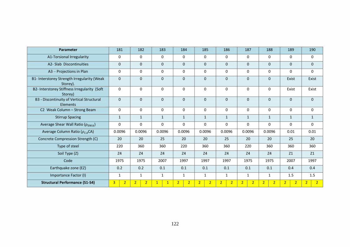
122
Parameter 181 182 183 184 185 186 187 188 189 190
A1-Torsional Irregularity 0 0 0 0 0 0 0 0 0 0
A2- Slab Discontinuities 0 0 0 0 0 0 0 0 0 0
A3 – Projections in Plan 0 0 0 0 0 0 0 0 0 0
B1- Interstorey Strength Irregularity (Weak Storey).
0 0 0 0 0 0 0 0 Exist Exist
B2- Interstorey Stiffness Irregularity (Soft Storey)
0 0 0 0 0 0 0 0 Exist Exist
B3 - Discontinuity of Vertical Structural Elements
0 0 0 0 0 0 0 0 0 0
C2 Weak Column – Strong Beam 0 0 0 0 0 0 0 0 0 0
Stirrup Spacing 1 1 1 1 1 1 1 1 1 1
Average Shear Wall Ratio ( ) 0 0 0 0 0 0 0 0 0 0
Average Column Ratio ( CA) 0.0096 0.0096 0.0096 0.0096 0.0096 0.0096 0.0096 0.0096 0.01 0.01
Concrete Compression Strength (C) 20 20 25 20 20 25 20 20 25 20
Type of steel 220 360 360 220 360 360 220 360 360 360
Soil Type (Z) Z4 Z4 Z4 Z4 Z4 Z4 Z4 Z4 Z1 Z1
Code 1975 1975 2007 1997 1997 1997 1975 1975 2007 1997
Earthquake zone (EZ) 0.2 0.2 0.1 0.1 0.1 0.1 0.1 0.1 0.4 0.4
Importance Factor (I) 1 1 1 1 1 1 1 1 1.5 1.5
Structural Performance (S1-S4) 3 2 2 2 1 1 2 2 2 2 2 2 2 2 2 2 2 2 2 2

123
Parameter 191 192 193 194 195 196 197 198 199 200
A1-Torsional Irregularity 0 0 0 0 0 0 0 0 0 0
A2- Slab Discontinuities 0 0 0 0 0 0 0 0 0 0
A3 – Projections in Plan 0 0 0 0 0 0 0 0 0 0
B1- Interstorey Strength Irregularity (Weak Storey).
0 0 0 0 0 0 0 0 1 1
B2- Interstorey Stiffness Irregularity (Soft Storey)
0 0 0 0 0 0 0 0 1 1
B3 - Discontinuity of Vertical Structural Elements
1 1 1 1 1 1 0 0 0 0
C2 Weak Column – Strong Beam 0 0 0 0 0 0 0 0 0 0
Stirrup Spacing 0 0 0 0 0 0 0 0 0 0
Average Shear Wall Ratio ( ) 0 0 0 0 0 0 0 0 0 0
Average Column Ratio ( CA) 0.01 0.01 0.01 0.01 0.01 0.01 0.01 0.01 0.01 0.01
Concrete Compression Strength (C) 20 25 20 20 20 25 20 20 20 20
Type of steel 220 360 360 220 360 360 360 220 360 220
Soil Type (Z) Z1 Z1 Z1 Z1 Z1 Z1 Z1 Z1 Z1 Z1
Code 1975 2007 1997 1975 1975 2007 1997 1975 1975 1975
Earthquake zone (EZ) 0.1 0.4 0.4 0.4 0.4 0.3 0.2 0.2 0.2 0.1
Importance Factor (I) 1.5 1.5 1.5 1.5 1.5 1.5 1.5 1.5 1.5 1.5
Structural Performance (S1-S4) 2 2 4 3 4 3 4 3 4 3 4 3 4 3 4 3 4 3 4 2

124
Parameter 201 202 203 204 205 206 207 208 209 210
A1-Torsional Irregularity 0 0 0 0 0 0 0 0 1 1
A2- Slab Discontinuities 0 0 0 0 0 0 0 0 0 0
A3 – Projections in Plan 0 0 0 0 0 0 0 0 0 0
B1- Interstorey Strength Irregularity (Weak Storey).
0 0 0 0 0 0 0 0 0 0
B2- Interstorey Stiffness Irregularity (Soft Storey)
0 0 0 0 0 0 0 0 1 1
B3 - Discontinuity of Vertical Structural Elements
0 0 0 0 0 0 0 0 0 0
C2 Weak Column – Strong Beam 0 0 0 0 0 0 0 0 0 0
Stirrup Spacing 1 1 1 1 1 1 1 1 1 1
Average Shear Wall Ratio ( ) 0 0 0 0 0 0 0 0 0 0
Average Column Ratio ( CA) 0.01 0.01 0.01 0.01 0.01 0.01 0.01 0.01 0.01 0.01
Concrete Compression Strength (C) 20 25 25 20 20 20 20 25 20 20
Type of steel 220 360 360 360 220 360 220 360 360 220
Soil Type (Z) Z1 Z1 Z1 Z1 Z1 Z1 Z1 Z1 Z2 Z2
Code 1975 1975 2007 1997 1975 1975 1975 2007 1997 1975
Earthquake zone (EZ) 0.4 0.4 0.3 0.2 0.2 0.2 0.1 0.4 0.4 0.4
Importance Factor (I) 1.5 1.5 1.5 1.5 1.5 1.5 1.5 1.5 1 1
Structural Performance (S1-S4) 4 4 3 3 2 2 2 1 3 2 2 2 2 2 3 2 3 2 4 2

125
Parameter 211 212 213 214 215 216 217 218 219 220
A1-Torsional Irregularity 1 1 1 1 1 1 1 1 1 1
A2- Slab Discontinuities 0 0 0 0 0 0 0 0 0 0
A3 – Projections in Plan 0 0 0 0 0 0 0 0 0 0
B1- Interstorey Strength Irregularity (Weak Storey).
0 0 0 0 0 0 0 1 1 1
B2- Interstorey Stiffness Irregularity (Soft Storey)
1 1 1 1 1 1 1 0 0 0
B3 - Discontinuity of Vertical Structural Elements
0 0 0 0 0 0 0 0 0 0
C2 Weak Column – Strong Beam 0 0 0 0 0 0 0 0 0 0
Stirrup Spacing 1 1 1 1 1 1 0 1 0 0
Average Shear Wall Ratio ( ) 0 0 0 0 0 0 0 0 0 0
Average Column Ratio ( CA) 0.0096 0.0096 0.0096 0.0096 0.0097 0.0096 0.0096 0.0094 0.0094 0.01
Concrete Compression Strength (C) 20 25 20 20 20 20 25 20 20 20
Type of steel 360 360 360 220 360 220 360 360 220 360
Soil Type (Z) Z1 Z2 Z1 Z1 Z1 Z1 Z1 Z1 Z1 Z1
Code 1975 2007 1997 1975 1975 1975 2007 1997 1975 1975
Earthquake zone (EZ) 0.4 0.3 0.2 0.2 0.2 0.1 0.4 0.4 0.4 0.4
Importance Factor (I) 1 1 1 1 1 1 1 1 1 1
Structural Performance (S1-S4) 4 3 3 2 3 1 3 1 3 1 3 1 4 2 4 2 4 4 3 2

126
Parameter 221 222 223 224 225 226 227 228 229 230
A1-Torsional Irregularity 1 1 1 1 1 0 0 0 0 0
A2- Slab Discontinuities 0 0 0 0 0 Case 1 Case 1 Case 1 Case 1 Case 1
A3 – Projections in Plan 0 0 0 0 0 0 0 0 0 0
B1- Interstorey Strength Irregularity (Weak Storey).
1 1 1 1 1 0 0 0 0 0
B2- Interstorey Stiffness Irregularity (Soft Storey)
0 0 0 0 0 0 0 0 0 0
B3 - Discontinuity of Vertical Structural Elements
0 0 0 0 0 0 0 0 0 0
C2 Weak Column – Strong Beam 0 0 0 0 0 0 0 0 0 0
Stirrup Spacing 0 0 0 0 0 1 1 1 1 1
Average Shear Wall Ratio ( ) 0 0 0 0 0 0 0 0 0 0
Average Column Ratio ( CA) 0.0093 0.0099 0.0096 0.0096 0.0096 0.0096 0.0096 0.0096 0.0098 0.0098
Concrete Compression Strength (C) 25 20 20 20 20 25 20 20 20 25
Type of steel 360 360 220 360 220 360 360 220 360 360
Soil Type (Z) Z1 Z1 Z2 Z2 Z1 Z1 Z1 Z1 Z1 Z1
Code 2007 1997 1975 1975 1975 2007 1997 1975 1975 2007
Earthquake zone (EZ) 0.3 0.2 0.2 0.2 0.1 0.4 0.4 0.4 0.4 0.3
Importance Factor (I) 1 1 1 1 1 1 1 1 1 1
Structural Performance (S1-S4) 4 2 2 2 2 1 2 1 2 1 2 2 2 2 3 4 2 4 2 2

127
Parameter 231 232 233 234 235 236 237 238 239 240
A1-Torsional Irregularity 0 0 0 0 0 0 0 0 0 0
A2- Slab Discontinuities Case 1 Case 1 Case 1 Case 1 0 0 0 0 0 0
A3 – Projections in Plan 0 0 0 0 1 1 1 1 1 1
B1- Interstorey Strength Irregularity (Weak Storey).
0 0 0 0 1 1 1 1 1 1
B2- Interstorey Stiffness Irregularity (Soft Storey)
0 0 0 0 1 1 1 1 1 1
B3 - Discontinuity of Vertical Structural Elements
0 0 0 0 1 1 1 1 1 1
C2 Weak Column – Strong Beam 0 0 0 0 0 0 0 0 0 0
Stirrup Spacing 1 1 1 1 1 0 0 0 0 0
Average Shear Wall Ratio ( ) 0 0 0 0 0.003 0 0 0 0 0
Average Column Ratio ( CA) 0.0096 0.0096 0.0096 0.0096 0.0096 0.0096 0.0096 0.0096 0.0096 0.0096
Concrete Compression Strength (C) 20 20 20 20 25 20 20 20 25 20
Type of steel 360 220 360 220 360 360 220 360 360 360
Soil Type (Z) Z1 Z1 Z1 Z2 Z1 Z3 Z3 Z4 Z4 Z3
Code 1997 1975 1975 1975 2007 1997 1975 1975 2007 1997
Earthquake zone (EZ) 0.2 0.2 0.2 0.1 0.4 0.4 0.4 0.4 0.3 0.2
Importance Factor (I) 1 1 1 1 1 1 1 1 1 1
Structural Performance (S1-S4) 2 2 2 2 2 2 2 1 4 2 4 3 4 3 4 3 4 3 4 3

128
Parameter 241 242 243 244 245 246 247 248 249 210
A1-Torsional Irregularity 0 0 0 1 1 1 1 1 1 1
A2- Slab Discontinuities Case1 Case1 Case1 0 0 0 0 0 0 0
A3 – Projections in Plan 1 1 1 0 0 0 0 0 0 0
B1- Interstorey Strength Irregularity (Weak Storey).
1 1 1 0 0 0 0 0 0 0
B2- Interstorey Stiffness Irregularity (Soft Storey)
1 1 1 0 0 0 0 0 0 0
B3 - Discontinuity of Vertical Structural Elements
1 1 1 0 0 0 0 0 0 0
C2 Weak Column – Strong Beam 1 1 1 0 0 0 0 0 0 0
Stirrup Spacing 0 0 0 1 1 1 1 1 1 1
Average Shear Wall Ratio ( ) 0 0 0 0 0 0 0 0 0 0
Average Column Ratio ( CA) 0.01 0.01 0.01 0.01 0.01 0.01 0.01 0.01 0.01 0.01
Concrete Compression Strength (C) 20 20 20 25 20 20 20 25 20 20
Type of steel 220 360 220 360 360 220 360 360 360 220
Soil Type (Z) Z1 Z1 Z1 Z1 Z1 Z1 Z1 Z1 Z1 Z1
Code 1975 1975 1975 2007 1997 1975 1975 2007 1997 1975
Earthquake zone (EZ) 0.2 0.2 0.1 0.4 0.4 0.4 0.4 0.3 0.2 0.2
Importance Factor (I) 1 1 1 1 1 1 1 1 1 1
Structural Performance (S1-S4) 4 3 4 3 3 1 2 2 2 2 4 3 4 3 2 2 2 2 3 2

129
Parameter 211 212 213 214 215 216 217 218 219 260
A1-Torsional Irregularity 1 1 1 1 1 1 1 1 1 1
A2- Slab Discontinuities 0 0 0 0 0 0 0 0 0 0
A3 – Projections in Plan 0 0 0 0 0 0 0 0 0 0
B1- Interstorey Strength Irregularity (Weak Storey).
0 0 0 0 0 0 0 0 0 0
B2- Interstorey Stiffness Irregularity (Soft Storey)
0 0 0 0 0 0 0 0 0 0
B3 - Discontinuity of Vertical Structural Elements
0 0 0 0 0 0 0 0 0 0
C2 Weak Column – Strong Beam 0 0 0 0 0 0 0 0 0 0
Stirrup Spacing 1 1 0 0 0 0 0 0 0 0
Average Shear Wall Ratio ( ) 0 0 0 0 0 0 0 0 0 0
Average Column Ratio ( CA) 0.01 0.01 0.01 0.01 0.01 0.01 0.01 0.01 0.01 0.01
Concrete Compression Strength (C) 20 20 25 20 20 20 25 20 20 20
Type of steel 360 220 360 360 220 360 360 360 220 360
Soil Type (Z) Z1 Z2 Z2 Z2 Z4 Z3 Z1 Z2 Z2 Z2
Code 1975 1975 2007 1997 1975 1975 2007 1997 1975 1975
Earthquake zone (EZ) 0.2 0.1 0.4 0.4 0.4 0.4 0.3 0.2 0.2 0.2
Importance Factor (I) 1 1 1 1 1 1 1 1 1 1
Structural Performance (S1-S4) 3 2 2 2 2 2 2 2 3 3 3 2 2 2 2 2 2 2 2 2