coherent financial cycles for g -7 countries: why ... · coherent financial cycles for g -7...

Coherent financial cycles for G-7 countries: Why extending credit can be an asset

Tuomas Peltonen* Deputy Head of the ESRB Secretariat

* with Yves Schüler (BuBa) and Paul Hiebert (IMF) The XII Annual Seminar on Risk, Financial Stability, and Banking of the Banco Central do Brazil Sao Paolo, 11 August 2017

DISCLAIMER: VIEWS EXPRESSED IN THIS PRESENTATION ARE THOSE OF THE PRESENTER AND DO NOT NECESSARILY REPRESENT THOSE OF

THE ESRB OR OF ITS MEMBER INSTITUTIONS, DEUTSCHE BUNDESBANK, OR THE IMF

The idea of the paper in brief, applied to financial cycles

“The business cycle is the phenomenon of a number of important economic aggregates […] being characterized by high pairwise coherences […].

This definition captures the notion of the business cycle as being a condition symptomizing the common movements of a set of aggregates.”

- T. Sargent (1987), Macroeconomic Theory, p. 282

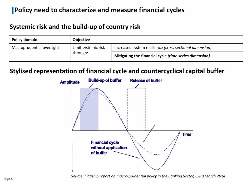
Policy need to characterize and measure financial cycles

Systemic risk and the build-up of country risk

Policy domain Objective

Macroprudential oversight Limit systemic risk through:

Increased system resilience (cross sectional dimension)

Mitigating the financial cycle (time series dimension)

Stylised representation of financial cycle and countercyclical capital buffer

Source: Flagship report on macro-prudential policy in the Banking Sector, ESRB March 2014

What do we do?

What do we do? 1. Propose a method to characterise and measure financial cycles through co-movement of credit and asset prices 2. Analyse and contrast properties of financial and business cycles for the G7 economies 3. Analyse financial cycles from a macroprudential perspective (early warning exercise)

What do we find?

What do we find? 1. The proposed method allows us to take into account important cross-country

differences in comovement of financial and economic indicators

2. Financial cycles are generally medium-term (8-20y), while business cycles are shorter (2-8y)

3. Financial cycles outperform single indicators and credit gap in predicting banking crises. Moreover, asset prices beyond house prices bring additional forecast power.

Literature

Overview of the recent literature on financial cycles

• Classical turning points algorithms: Claessens et al. (2011,2012); Hiebert et al. (2014)

• Filtered medium-term cycles, e.g., 8-30 years: Drehmann et al. (2012); Borio (2014), Aikman et al. (2015); Stremmel (2015)

• Unobserved components models: Rünstler and Vlekke (2016); Galati et al. (2016)

• Wavelets: Verona (2016)

• Indirect spectrum estimation: Strohsal et al. (2015a,b)

• Direct spectral analysis, multiple detrending procedures: Schüler (forthcoming)

Our work is also related to literature on financial crises prediction • Financial crises prediction: Borio and Lowe (2004), Schularick and Taylor (2012), Behn et al.

(2013), Jordà et al. (2015), Anundsen et al. (2016)

1

2

8

Measurement: Variables and Methodology

5 Summary

Background and research questions

3 Properties: Across countries and relative to business cycles

Presentation outline

4 Composite cycles: Construction, evaluation, and policy-relevance

Measurement: Variables – role for asset prices

Credit as a necessary element of a financial cycle! • Credit as source of financial instability and not only amplifier (Minsky 1977) • Financial recessions follow credit booms (Schularick and Taylor 2012, Jordà et al.

2013; Boissay et al. 2016)

Is it sufficient?

• Not all credit booms end in financial recessions (Mendoza and Terrones 2008; Gorton and Ordoñez 2015)

Role for asset prices? Credit and asset prices jointly matter! • Leveraged bubbles detrimental (Fisher 1933; Jordà et al. 2015) • Credit market frictions imply the state of balance sheet matters for borrowing

• leverage cycles (Geanakopolos 2010), • real estate as collateral constraint (Iacoviello 2005), • equity prices and corporate bonds and their role for firms’ balance sheets

(Gilchrist et al 2009 and 2012; Claessens et al. 2012 and 2011; Hubrich and Tetlow 2015; Fink and Schüler 2015)

• Evidence of global financial cycle in asset prices (Rey 2015)

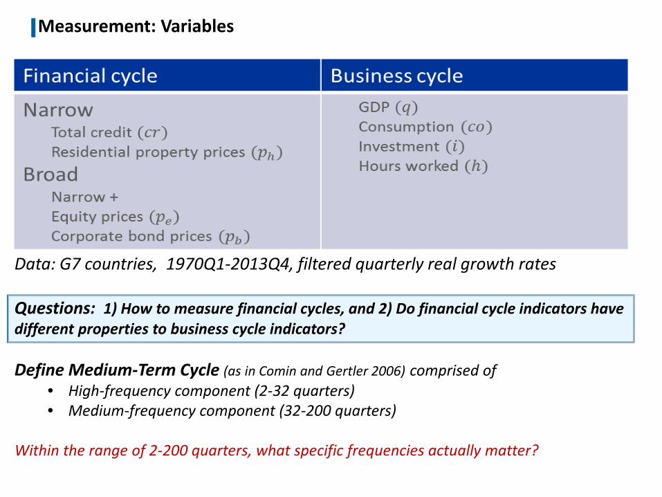
Measurement: Variables

Data: G7 countries, 1970Q1-2013Q4, filtered quarterly real growth rates Questions: 1) How to measure financial cycles, and 2) Do financial cycle indicators have different properties to business cycle indicators? Define Medium-Term Cycle (as in Comin and Gertler 2006) comprised of

• High-frequency component (2-32 quarters) • Medium-frequency component (32-200 quarters)

Within the range of 2-200 quarters, what specific frequencies actually matter?

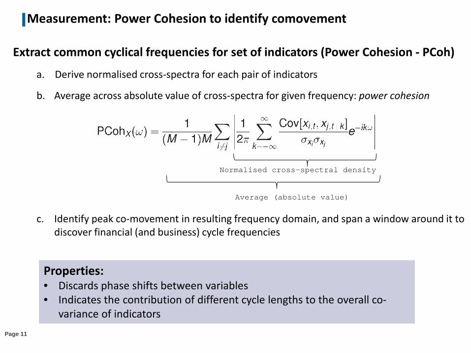
Measurement: Power Cohesion to identify comovement

Extract common cyclical frequencies for set of indicators (Power Cohesion - PCoh)

a. Derive normalised cross-spectra for each pair of indicators

b. Average across absolute value of cross-spectra for given frequency: power cohesion

c. Identify peak co-movement in resulting frequency domain, and span a window around it to discover financial (and business) cycle frequencies

Normalised cross-spectral density

Average (absolute value)

Properties: • Discards phase shifts between variables • Indicates the contribution of different cycle lengths to the overall co-

variance of indicators

1

2

12


5 Summary





Properties: Pairwise comovement of indicators (cross-spectra) Cross-spectra for US – financial cycle vs business cycle *Medium-term cycles for financial cycle indicators * Shorter-term cycles for business cycle indicators *Amplitude of financial cycles much larger

Notes: This panel shows the absolute cross-spectra of the financial and business cycle indicators. The x-axis measures the frequencies of cycles from 1.25 - 50 years. The blue area depicts business cycle frequencies, i.e., cycles with durations of 2-8 years and the purple area marks frequencies important for financial cycles (8-20 years). Page 9

Properties: Peak comovement of financial and business cycle indicators

Power cohesion (PCoh) for US – financial cycle vs business cycle *Broad and narrow financial cycle frequencies clearly medium-term *Short-term frequencies almost muted for financial cycles

Notes: This graph shows the measure power cohesion of the narrow and broad financial cycle as well as the business cycle. Broad refers to the inclusion of all indicators, i.e., credit, house, equity, and bond prices, whereas narrow is defined by house prices and credit only. The dashed lines indicate the 68% bootstrapped confidence intervals. The x-axis measures the frequencies of cycles from 1.25 to 50 years. The blue area depicts business cycle frequencies, i.e., cycles with durations of 2-8 years and the purple area (8-20 years) marks frequencies most important for financial cycles

Properties: Ranges for financial and business cycles

Notes: This graph depicts the 25% highest density region of power cohesion excluding cycles lower than 5 quarters for financial and business cycle indicators. The white dash locates the peak of power cohesion. The purple region marks medium-term frequencies and the blue area short-term fluctuations.

25% of highest power cohesion (PCoh) region of G7 countries *Medium-term (8-20y) duration of broad and narrow financial cycles *Mostly short-term (8-2y) duration of business cycles *Heterogeneity across countries

1

2

16


5 Summary





Composite cycles: Construction of composite financial cycle indicator

Create composite financial cycle index and cycles for constituent components 1. Standardise indicators using the empirical cumulative distribution function (ecdf)

2. Filter and aggregate using time-varying correlations

a) Band pass filter indicators using country-specific financial cycle frequencies

b) Real time aggregate index using asymmetric moving average (positive correlations)

1.

2.

Composite cycles: Examples of US financial and business cycles

(c) Real time composite cycle indices

Notes: This panel shows the US composite financial and business cycles in standardised growth rates, where 0.5 denotes the historical median after removing a nonlinear trend; 0 is the smallest and 1 the largest growth rate observed in a country’s history. Filtering is done using the Christiano and Fitzgerald (2003) band-pass filter employing country specific frequency windows. Real time cycles are derived using an asymmetric moving average. Grey area indicates NBER recession dates.

Composite cycles: Evaluation and policy-relevance

Early-warning signalling exercise to predict banking crises Goal:

• Compare performance of financial cycles vs indicators and credit-to-GDP gap

Setup: • G-7 countries, 10 year training sample for ecdf (effective sample: 1980Q1-

2013Q4)

• Quarterly Laeven and Valencia (2012) systemic banking crises dates • Two signalling events (1-at event; 0-otherwise):

• Start of crisis • 1-4 quarters vulnerability period ahead of crisis

• Pooled logit model: One quarter pseudo-out-of sample exercise + In-sample • Out-of-sample period: 2000Q1-2013Q4

Results: • Financial cycle (broad) is the best indicator both out-of-sample and in-sample

prediction of banking crises • Both financial cycle measures outperform single indicators, credit gap and business

cycle in banking crisis prediction

Composite cycles: Evaluation and policy-relevance

Notes: Table shows results of the out-of- and in-sample exercise as described in Section 4.4.1. “Observ.” refers to observations, “TP” to true positive, “FP” to false positive, “TN” to true negative, “FN” to false negative, “TI” to Type I error, “TII” to Type II error, “Ur ” to relative usefulness, “NtS” to noise-to-signal ratio, and “AUC” to area under the curve. “-“ indicates that the statistic is not defined

Early warning signalling exercise (cont’d)

1

2

21


5 Summary


3 Properties: Financial and business cycles within and across countries



Summary

Propose a method to analyse financial cycles through co-movement of credit and asset prices

∙ Motivated through leverage cycles and the detrimental effects of leveraged bubbles

∙ Provide method to analyse the properties of financial cycles

Contrast properties of financial and business cycle

∙ Financial cycles differ from business cycles within countries (dominant medium-term)

∙ Financial cycles differ across countries.

Scope for country-specific and differentiated countercyclical policies

Policy-relevance:

∙ Composite financial cycle of credit and asset prices outperforms single indicators and credit-to-GDP gap in predicting banking crises.

Coherent financial cycles for G-7 countries: Why extending credit can be an asset

Tuomas Peltonen* Deputy Head of the ESRB Secretariat

* with Yves Schüler and Paul Hiebert The XII Annual Seminar on Risk, Financial Stability, and Banking of the Banco Central do Brazil Sao Paolo, 11 August 2017

References: ∙ Aikman, D., Haldane, A. and Nelson, B.: 2015, Curbing the credit cycle, The Economic Journal 125, 1072–1109. ∙ Anundson, A., Gerdrup, K., Hansen, F. and Kragh-Sørensen, K.: 2016, Bubbles and crises: The role of house prices and credit,

Journal of Applied Econometrics 31, 1291–1311. ∙ Behn, M., Detken, C., Peltonen, T. and Schudel, W.: 2013, Setting countercyclical capital buffers based on early warning

models: Would it work?, ECB Working Paper 1604. ∙ Boissay, F., Collard, F. and Smets, F.: 2016, Booms and banking crises, Journal of Political Economy 124, 489–538. ∙ Borio, C.: 2014, The financial cycle and macroeconomics: What have we learnt?, Journal of Banking and Finance 45, 182–

198. ∙ Borio, C. and Lowe, P.: 2004, Securing sustainable price stability: Should credit come back from the wilderness?, BIS

Working Papers No 157. ∙ Claessens, S., Kose, M. and Terrones, M.: 2011, Financial cycles: What? How? When?, IMF Working Paper WP/11/76 . ∙ Claessens, S., Kose, M. and Terrones, M.: 2012, How do business and financial cycles interact?, Journal of International

Economics 87, 178–190. ∙ Comin, D. and Gertler, M.: 2006, Medium-term business cycles, American Economic Review 96, 523–551. ∙ Drehmann, M., Borio, C. and Tsatsaronis, K.: 2012, Characterising the financial cycle: Don‘t lose sight of the medium term!,

BIS Working Paper 380. ∙ Fink, F. and Schüler, Y.: 2015, The transmission of US systemic financial stress: Evidence for emerging market economies,

Journal of International Money and Finance 55, 6–26. ∙ Galati, G., Hindrayanto, I., Koopman, S. and Vlekke, M.: 2016, Measuring financial cycles with a model-based filter:

Empirical evidence for the United States and the euro area, Economics Letters 145, 83–87. ∙ Geanakopolos, J.: 2010, The leverage cycle, in D. Acemoglu, K. Rogoff and M.Woodford (eds), NBER Macroeconomics

Annual 2009, Volume 24, University of Chicago Press, Chicago, chapter 1, pp. 1–65. ∙ Gilchrist, S., Yankov, V. and Zakrajšek, E.: 2009, Credit market shocks and economic fluctutations: Evidence from corporate

bond and stock markets, Journal of Monetary Economics 56, 471–493. ∙ Gilchrist, S. and Zakrajšek, E.: 2012, Credit spreads and business cycle fluctuations, American Economic Review 102, 1692–

1720. ∙ Gorton, G. and Ordoñez, G.: 2016, Good booms, bad booms, NBER Working Paper 22008. ∙ Hiebert, P., Klaus, B., Peltonen, T., Schüler, Y. and Welz, P.: 2014, Capturing the financial cycle in the euro area, Financial

Stability Review: Special Feature B. ∙ Hubrich, K. and Tetlow, R.: 2015, Financial stress and economic dynamics: The transmission of crises, Journal of Monetary

Economics 70, 100–115.

References

References (cont’d): ∙ Iacoviello, M.: 2005, House prices, borrowing constraints, and monetary policy in the business cycle, American Economic

Review 95, 739–764. ∙ Jaccard, I.: forthcoming, Asset pricing and the propagation of macroeconomic shocks, Journal of the European Economic

Association . ∙ Jordà, O., Schularick, M. and Taylor, A. M.: 2013, When credit bites back, Journal of Money, Credit and Banking 45, 3–28. ∙ Jordà, O., Schularick, M. and Taylor, A. M.: 2015, Leveraged bubbles, Journal of Monetary Economics 76, S1–S20. ∙ Laeven, L. and Valencia, F.: 2012, Systemic banking crises database: An update, IMF Working Paper WP/12/163. ∙ Mendoza, E. and Terrones, M.: 2008, An anatomoy of credit booms: Evidence from macro aggregates and micro data, NBER

Working Paper 14049. ∙ Minsky, H.: 1977, The financial instability hypothesis: An interpretation of Keynes and an alternative to “standard” theory,

Nebraska Journal of Economics and Business 16, 5–16. ∙ Rey, H.: 2015, Dilemma not trilemma: The global financial cycle and monetary policy independence, NBER Working Paper

21162. ∙ Rünstler, G. and Vlekke, M.: 2016, Business, housing and credit cycles, ECB Working Paper 1915. ∙ Schüler, Y.: forthcoming, Detrending and financial cycle facts across G7 countries: Mind a spurious medium term!, ECB and

Bundesbank Working Paper. ∙ Schularick, M. and Taylor, A.: 2012, Credit booms gone bust: Monetary policy, leverage cycles, and financial crises, 1870-

2008, American Economic Review 102, 1029–1061. ∙ Stremmel, H.: 2015, Capturing the financial cycle in Europe, ECB Working Paper 1811. ∙ Strohsal, T., Proaño, C. and Wolters, J.: 2015a, Characterizing the financial cycle: Evidence from a frequency domain analysis,

Deutsche Bundesbank Discussion Paper 22/2015. ∙ Strohsal, T., Proaño, C. and Wolters, J.: 2015b, How do financial cycles interact? Evidence for the US and the UK, SFB 649

Discussion Paper 2015-024. ∙ Verona, F.: 2016, Time-frequency characterization of the U.S. financial cycle, Economics Letters 144, 75–79.

References

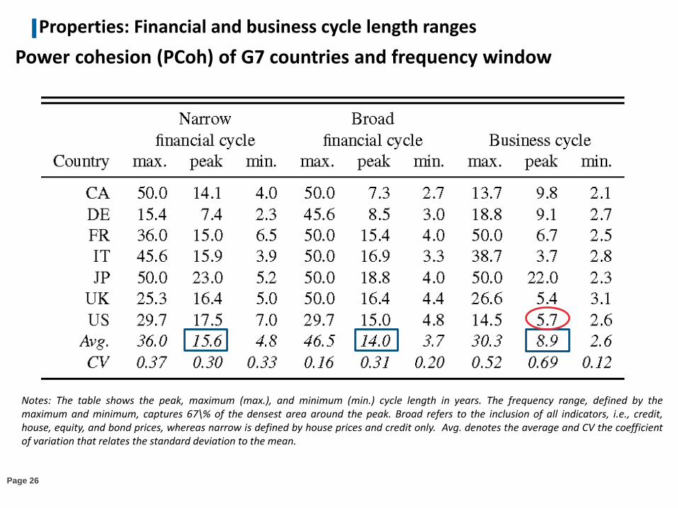
Properties: Financial and business cycle length ranges

Power cohesion (PCoh) of G7 countries and frequency window

Notes: The table shows the peak, maximum (max.), and minimum (min.) cycle length in years. The frequency range, defined by the maximum and minimum, captures 67\% of the densest area around the peak. Broad refers to the inclusion of all indicators, i.e., credit, house, equity, and bond prices, whereas narrow is defined by house prices and credit only. Avg. denotes the average and CV the coefficient of variation that relates the standard deviation to the mean.

coherent financial cycles for g -7 countries: why ... · coherent financial cycles for g -7...

Documents