cognitive radio mobile ad hoc networks || delay in cognitive radio networks

Chapter 10Delay in Cognitive Radio Networks

Yaling Yang, Chuan Han, and Bo Gao

Abstract This chapter presents analysis for delays for both multihop cognitiveradio networks and single-hop cognitive radio networks. For multihop cognitiveradio networks, we analyze the amount of time that a packet spends to travel overthe intermittent relaying links over multiple relaying hops and characterize it withthe metric called information propagation speed. Optimal relaying node placementstrategies are derived to maximize information propagation speed. For single-hopcognitive radio networks, we will analyze how delay is affected by multiple cog-nitive radio design options, including the number of channels to be aggregated,the duration of transmission, the channel separation constraint on channel aggre-gation, and the time needed for spectrum sensing and protocol handshake. Howthese different options may affect the delay under different secondary and primaryuser traffic loads is revealed. Methods for computing optimal cognitive radio designand operation strategy are derived.

10.1 Introduction

Cognitive radio networks (CRN) have a lot of potentials to improve wireless spec-trum efficiency. Understanding the fundamental performance characteristics of thisnew type of networks is important for the optimal planning of CRN and the designof CRN applications. Hence, in this chapter, one important aspect of CRN perfor-mance, the delay, is analyzed.

For a multihop CRN, information propagation speed (IPS) is used as a metric forunderstanding the multihop end-to-end packet delays. Models of IPS and methodsto maximize IPS in two cases are introduced. The first case, named the maximumnetwork IPS, maximizes IPS across a network topology over an infinite plane. Thesecond case, named the maximum flow IPS, maximize the IPS between a given pairof source and destination nodes separated by a fixed distance. The analysis showsthat both maximum IPS are determined by the activity level of primary users (PU)and the placement of secondary user (SU) nodes. Optimal relay placement strategieswill be identified to maximize these two IPS under different primary users’ activitylevels.

Y. Yang (B)Virginia Polytechnic Institute and State University, Blacksburg, VA, USAe-mail: [email protected]

F.R. Yu (ed.), Cognitive Radio Mobile Ad Hoc Networks,DOI 10.1007/978-1-4419-6172-3_10, C© Springer Science+Business Media, LLC 2011

249

250 Y. Yang et al.

For a single-hop CRN, we will analyze how delay is affected by multiple SUdesign options, including the number of channels to be aggregated, the duration oftransmission, the channel separation constraint on channel aggregation, and the timeneeded for spectrum sensing and protocol handshake. How these different optionsmay affect the delay under different SU and PU traffic loads is revealed. Methodsfor computing optimal CRN design and operation strategy are derived.

10.2 Optimal Information Propagation Speed Analysisin Multihop Cognitive Radio Networks

Similar to the delay in any networks, delay in CRN is the combination of two com-ponents [1]: the information propagation delay and the queuing delay. The informa-tion propagation delay is the amount of time that a packet spends to travel over theintermittent relaying links in a CRN and is determined by the underlying commu-nication capabilities of the network. The queuing delay is the amount of time thata packet spends in waiting for other packets to finish their transmission. Queuingdelay is determined by the specific traffic load, traffic pattern, and the schedulingalgorithms adopted at all hops of CRN.

In this section, we will study the information propagation delay and under-stand how to plan node placement to minimize this important delay component inmultihop CRN. The analysis of information propagation delay in CRN is differentfrom it in other types of networks due to the unique two-tier architecture of CRN,where the information propagation delay in a CRN is related to not only the settingsof the CRN network itself but also the traffic activities of primary users. Hence,existing works about multihop delay analysis for other types of networks [1–4]cannot be applied to CRN.

As a means to interpret the information propagation delay independent of prop-agation distance, we use Information Propagation Speed (IPS) as its measurementmetric. Information propagation speed is defined as the speed that a piece of infor-mation (e.g., a packet of very small size) can be transmitted over a multi-hop CRN.In the remainder of this section, we will establish a model of IPS in CRN and catego-rize IPS maximization problem into two cases. The first case, named the maximumnetwork IPS problem, maximizes IPS across a network topology over an infiniteplane. The second case, named the maximum flow IPS problem, maximizes the IPSbetween a given pair of source and destination nodes separated by a fixed distance.We will reveal that both maximum network and flow IPS are determined by theprimary user (PU) activity level and the placement of SU relay nodes. We will intro-duce numerical methods to compute the two maximum IPS and built optimal relayplacement strategies to realize these two maximum IPS under different PU activitylevels.

The results of the IPS study can be used as a benchmark for network design.It can be used to check whether a certain delay-sensitive traffic is supportable in a

10 Delay in Cognitive Radio Networks 251

particular network setting. The optimal node placement settings that can achieve themaximum IPS can also be used as useful design guidelines in CRN planning.

The rest of this section is organized as follows. The network model and IPSmodel are presented in Sections 10.2.1 and 10.2.2. The analyses for the networkand flow IPS are in Sections 10.2.3 and 10.2.4, respectively. The analytical resultsare validated by simulations and numerical results in Section 10.2.5.

10.2.1 Network Model

A cognitive radio network is modeled as a network formed by secondary users (SU)and an overlaid primary user (PU) network in an infinite two-dimensional region.The location distribution of PU nodes is assumed to be a two-dimensional Poissonpoint processes. Assume that there are K channels and an active PU or SU only usesone channel. Based on the measurement study of realistic wireless PU activities incellular networks [5], the PU traffic can be accurately modeled as a Poisson arrivalprocess with the mean arrival rate λP per unit area, while the service time of PU isusually not Poisson.

We assume duplex communications between the SU transmitter and the receiver(e.g., the SU receiver sends ACK back for received data). Hence, both SU transmit-ter and SU receiver need to avoid interfering with PU receivers. Denote ds as thesensing radius of SU for PU receivers1 and let U (d) be the union of the sensingregions of a pair of SU transmitter and receiver that are d distance apart. The shapeof U (d) is shown by the gray region in Fig. 10.1 (II). When there are no active PUreceivers within U (d), the SU transmitter and receiver can communicate and we callthat the SU link between the SU transmitter and the receiver is feasible. Note thathere we implicitly assume that SUs can cancel the interference from PU transmittersto the SU receiver through interference cancelation schemes [6].

(I) (II)

SU Tx SU Rx PU RxSU Tx

ds

dSU Rx PU Rx

ds

d

Fig. 10.1 One hop sensing region

1 PU receiver detection can be realized by exploiting the feedback mechanisms in two-way PUcommunications as shown by [7, 8].

252 Y. Yang et al.

It is important to note that given cognitive radio’s capability to adapt transmissionpower and hence its potential interference to PUs, the sensing radius of SU shouldnot be treated as a fixed value. In our model, we assume that a SU controls itstransmit power so that its communication range equals its distance d to its receiver.In this way, the interference to PUs is minimized. Under this optimal power controlpolicy, we get:

Pt

dα= Tr (10.1)

where α ≥ 2 is the attenuation exponent, Pt is the transmit power of the SU trans-mitter and Tr is the receiver’s sensitivity level. Assume that when the signal of a SUexceeds the interference threshold Ts at a PU receiver, the PU receiver is interferedby the SU transmission. Therefore, SU’s sensing radius ds can be expressed as:

Pt

dαs= Ts (10.2)

Combining (10.1) and (10.2), we have

ds =(

Tr

Ts

) 1α

d = C1d (10.3)

where C1 =(

TrTs

) 1α

. The above equation shows that the sensing radius ds is propor-

tional to the SU communication range that equals the distance d between the SUtransmitter and SU receiver under the optimal power control policy.

10.2.2 Problem Formulation

Based on the assumptions in the previous section, we can model IPS, denoted as w,in a multihop CRN as:

w = D

τ(D)=

∑i P(di )∑i τ(di )

(10.4)

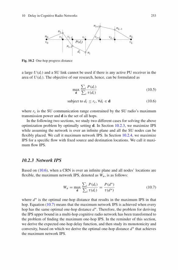
where D is the distance between a pair of SU source node and destination node, andτ(D) is the expected information propagation delay over this distance D. di is thetransmission distance of the i th hop, and P(di ) is the projection of di on the straightline from the source to the destination as shown in Fig. 10.2. τ(di ) is the expectedinformation propagation delay over the i th hop.

By observing (10.4), we could see a trade-off exists in the setting of di and w.While a large di increases the numerator in (10.4), it also increase τ(di ) since it has


n0

v0

v1 vi–1

ni+1 nL–1

nL

vL

vL–1vi+1

ni–1

di ni

n1

vi

P(di)

Fig. 10.2 One-hop progress distance

a large U (di ) and a SU link cannot be used if there is any active PU receiver in thearea of U (di ). The objective of our research, hence, can be formulated as

maxd


(10.5)

subject to di ≤ rc,∀di ∈ d (10.6)

where rc is the SU communication range constrained by the SU radio’s maximumtransmission power and d is the set of all hops.

In the following two sections, we study two different cases for solving the aboveoptimization problem by optimally setting d. In Section 10.2.3, we maximize IPSwhile assuming the network is over an infinite plane and all the SU nodes can beflexibly placed. We call it maximum network IPS. In Section 10.2.4, we maximizeIPS for a specific flow with fixed source and destination locations. We call it maxi-mum flow IPS.

10.2.3 Network IPS

Based on (10.6), when a CRN is over an infinite plane and all nodes’ locations areflexible, the maximum network IPS, denoted as Wu , is as follows:

Wu = maxd


= P(d∗)τ (d∗)

(10.7)

where d∗ is the optimal one-hop distance that results in the maximum IPS in thathop. Equation (10.7) means that the maximum network IPS is achieved when everyhop has the same optimal one-hop distance d∗. Therefore, the problem for derivingthe IPS upper bound in a multi-hop cognitive radio network has been transformed tothe problem of finding the maximum one-hop IPS. In the reminder of this section,we derive the expected one-hop delay function, and then study its monotonicity andconvexity, based on which we derive the optimal one-hop distance d∗ that achievesthe maximum network IPS.

254 Y. Yang et al.

10.2.3.1 One-Hop Delay Function

The expected one-hop delay over a transmission distance d can be expressed as

τ(d) = E{T } + τ0 (10.8)

where E{T } is the mean one-hop delay induced by waiting for PU traffic to vacanta channel, τ0 is the sum of other constant delay components, such as channel sens-ing delay for determining the channel availability, transmission delay determinedby the channel capacity, and packet processing delay determined by the hardwareprocessing capability.

While τ0 is fixed given the cognitive radio design, the value of E{T } is equivalentto the time that it takes for a channel to be vacanted by PU when a SU is ready totransmit a packet. Note that in Section 10.2.1, we have pointed out that measure-ment results [5] show that realistic PU traffic follows a Poisson arrival process andhas complex service time distribution. Hence, we can treat PU as a high priorityflow, SU as a low priority flow, and the K channels as K servers in a two-prioritypreemptive M/G/K queuing model. Under this model, E{T } is equivalent to thequeueing delay of the low priority flow when the packet service time of the lowpriority flow approaches 0.

The anlaytical work of two-priority preemptive M/G/K queue in [9] shows thatthe queuing delay of the low priority flow can be approximated as follows:

delay1 =

⎧⎪⎪⎪⎪⎪⎪⎪⎪⎪⎪⎪⎪⎪⎪⎪⎪⎪⎨⎪⎪⎪⎪⎪⎪⎪⎪⎪⎪⎪⎪⎪⎪⎪⎪⎪⎩

1

2Kρ1

[s1ρ1 + s2ρ2

1− ρ1 − ρ2

(ρ1 + ρ2)K + (ρ1 + ρ2)

2− s2ρ2

1− ρ2

ρK2 + ρ2

2

]

ρ2 > 0.7, ρ1 + ρ2 > 0.7;1

2Kρ1

[s1ρ1 + s2ρ2

1− ρ1 − ρ2

(ρ1 + ρ2)K + (ρ1 + ρ2)

2− s2ρ2

1− ρ2ρ

K+12

2

]ρ2 < 0.7, ρ1 + ρ2 > 0.7;

1

2Kρ1

[s1ρ1 + s2ρ2

1− ρ1 − ρ2(ρ1 + ρ2)

K+12 − s2ρ2

1−ρ2ρ

K+12

2

]

ρ2 < 0.7, ρ1 + ρ2 < 0.7.(10.9)

where subscript 1 is for low priority flow and 2 is for high priority flow and si :=1+C2

Biμi

,C2Bi:= σ 2

i

X̄i2 , ρi := λi X̄i/K Here, Xi is the service time for priority i traffic,

σ 2i is the variance of Xi , and X̄i is the mean value of Xi .

Therefore, assuming that the traffic load of PU is reasonable (a.k.a. ρ2 < 0.7),we can get E{T } as

E{T } = limρ1→0,s1→0

delay1 (10.10)


=K+1

2 s2ρK+1

22

2K (1− ρ2)+ s2ρ

K+32

2

2K (1− ρ2)2(10.11)

The reason that we assume ρ2 < 0.7 is because CRN is usually used in scenarioswhere PUs have low utilization of licensed spectrum bands. Hence, the assumptionthat PU traffic load is light to medium is valid in our application scenario. The ρ2 in(10.11) can be computed as follows. Note that within an unit area, the PU traffic isa Poisson arrival process with parameter λP. Hence, the aggregate PU traffic arrivalrate within region U (d) is Poisson with parameter λa = λP A(d), where A(d) isthe area of region U (d) as shown in Fig. 10.1. By (10.3) and Fig. 10.1 (II), it can

be shown that A(d) = Cd2, where C = 2πC21 − 2C2

1 cos−1 12C1

+√

C21 − 1

4 and

C1 =(

TrTs

) 1α

. Therefore, we have

ρ2 = Cd2λP X̄ p/K = Cd2ρ (10.12)

where ρ := λP X̄ p/K and X̄ p is the mean active duration of a primary user.Hence, combining (10.11) and (10.8), we get:

τ(d) = (K + 1)s2ρK+1

22

4K (1− ρ2)+ s2ρ

K+32

2

2K (1− ρ2)2+ τ0 (10.13)

10.2.3.2 Properties of One-Hop Delay Function

Next, we study two important properties of τ(d): monotonicity and convexity. Weshow that the one-hop delay function τ(d) is monotonically increasing and strictlyconvex. To simplify the mathematical derivation, we denote

h1(ρ2) = (K + 1)s2ρK+1

22

4K (1− ρ2)(10.14)

and

h2(ρ2) = s2ρK+3

22

2K (1− ρ2)2(10.15)

We can prove the following lemmas.

Lemma 1 For (10.14) and (10.15), it follows

h′1(ρ2) > 0, h′2(ρ2) > 0 (10.16)

256 Y. Yang et al.

and

h′′1(ρ2) > 0, h′′2(ρ2) > 0 (10.17)

Proof See our technical report [10].

Lemma 2 The function τ(d), 0 < d ≤ rc is monotonically increasing.


Lemma 3 The function τ(d), 0 ≤ d ≤ rc is strictly convex.


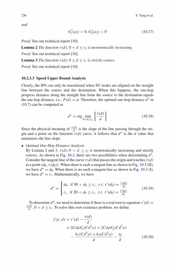
10.2.3.3 Speed Upper Bound Analysis

Clearly, the IPS can only be maximized when SU nodes are aligned on the straightline between the source and the destination. When this happens, the one-hopprogress distance along the straight line from the source to the destination equalsthe one hop distance, i.e., P(d) = d. Therefore, the optimal one-hop distance d∗ in(10.7) can be computed as

d∗ = arg min0<d≤rc

{τ(d)

d

}(10.18)

Since the physical meaning of τ(d)d is the slope of the line passing through the ori-

gin and a point on the function τ(d) curve, it follows that d∗ is the d value thatminimizes the line slope.

• Optimal One-Hop Distance AnalysisBy Lemma 2 and 3, τ(d), 0 < d ≤ rc is monotonically increasing and strictlyconvex. As shown in Fig. 10.3, there are two possibilities when determining d∗.Consider the tangent line of the curve τ(d) that passes the origin and touches τ(d)at a point (d0, τ (d0)). When there is such a tangent line as shown in Fig. 10.3 (II),we have d∗ = d0. When there is no such a tangent line as shown in Fig. 10.3 (I),we have d∗ = rc. Mathematically, we have

d∗ =⎧⎨⎩

d0, if ∃0 < d0 ≤ rc, s.t. τ ′(d0) = τ(d0)d0

rc, if �0 < d0 ≤ rc, s.t. τ ′(d0) = τ(d0)d0

(10.19)

To determine d∗, we need to determine if there is a real root to equation τ ′(d) =τ(d)

d , 0 < d ≤ rc. To solve this root existence problem, we define

f (ρ, d) = τ ′(d)− τ(d)

d= 2Cdρh′1(Cd2ρ)+ 2Cdρh′2(Cd2ρ)

− h1(Cd2ρ)+ h2(Cd2ρ)

d− τ0

d(10.20)


(I)0 d

(d) (d)

d0 rc rc0 d(II)

Fig. 10.3 Two examples of τ(d): (I) ∃0 < d0 ≤ rc, s.t. τ ′(d0) = τ(d0)d0

; (II) �0 < d0 ≤rc, s.t. τ ′(d0) = τ(d0)

d0

and study the root existence problem for the following equation

f (ρ, d) = 0, 0 < d ≤ rc (10.21)

• Threshold Property of d∗Next, let us solve the root existence problem in (10.21) and determine d∗. Theanalytical results are summarized in the following proposition.

Proposition 1 There exists a threshold 0 < ρu(rc) <1

Cr2c, f (ρu(rc), rc) = 0 such

that d∗ = rc when ρ < ρu(rc) and d∗ < rc when ρ > ρu(rc).

Proof By Lemma 2 and 3, τ(d), 0 < d ≤ rc is monotonically increasing and strictlyconvex. By (10.20), it follows that f (ρ, d) is an increasing function of d. Sincelim

d→0+f (ρ, d) = −∞, it follows that f (ρ, d) increases from −∞ to f (ρ, rc) when

d increases from 0 to rc. When f (ρ, rc) > 0, there must exist a real root to theproblem in (10.21). By (10.19), we have d∗ < rc. When f (ρ, rc) < 0, we havef (ρ, d) < 0,∀0 < d ≤ rc, i.e., there does not exist a real root to the problem in(10.21). By (10.19), we have d∗ = rc.

Next, we study the positivity of f (ρ, rc). Since rc is fixed, the positivity off (ρ, rc) depends on ρ. We study the positivity of f (ρ, rc) when ρ changes. By(10.20), we have

f (ρ, rc) = 2Crcρh′1(

Cr2c ρ

)+ 2Crcρh′2

(Cr2

c ρ)

− h1(Cr2

c ρ)+ h2

(Cr2

c ρ)

rc− τ0

rc(10.22)

It can be shown that limρ→0+ f (ρ, rc) < 0 and limρ→

(1

Cr2c

)− f (ρ, rc) = ∞.

Therefore, there is at least one real root to equation

f (ρ, rc) = 0, 0 < ρ <1

Cr2c

(10.23)

258 Y. Yang et al.

In the following, we prove that there is only one real root. By (10.22), we have

∂ f (ρ, rc)

∂ρ= Crch′1

(Cr2

c ρ)+ Crch′2

(Cr2

c ρ)

+ 2ρC2r3c h′′1

(Cr2

c ρ)+ 2ρC2r3

c h′′2(

Cr2c ρ

)(10.24)

By (10.16) and (10.17) in Lemma 1, we have ∂ f (ρ,rc)∂ρ

> 0, i.e., f (ρ, rc) is anincreasing function with respect to ρ. Therefore, there exists only one real rootto equation f (ρ, rc) = 0, 0 < ρ < 1

Cr2c

. Denote the root as ρu(rc). Recall

that limρ→0+ f (ρ, rc) < 0 and limρ→

(1

Cr2c

)− f (ρ, rc) = ∞. It follows that

f (ρ, rc) > 0 when ρ > ρu(rc) and f (ρ, rc) < 0 when ρ < ρu(rc). Therefore,when ρ > ρu(rc) we have d∗ < rc, and when ρ < ρu(rc) we have d∗ = rc.

Although it is difficult to derive a closed form formula for the threshold ρu(rc)

and d∗, we can numerically derive it from (10.23). The physical intuition behindProposition 1 is as follows. When the actual ρ is small, the delay of SU traffic causedby yielding to PU transmissions in the region U (d) is negligible. The SU’s IPS isonly constrained by the maximum transmission power. Therefore, the optimal one-hop distance d∗ = rc. When ρ is large, the delay caused by PU transmissions in theregion U (d) dominates other delay components. Hence, a shorter one-hop distanced incurs a smaller U (d) size, resulting a smaller delay. Therefore, the optimal one-hop distance d∗ < rc.

10.2.4 Flow IPS

Beyond the network IPS upper bound for all possible flows, we are also interestedin the IPS upper bound for a particular given flow, called the flow IPS upper bound.Since in this case the source–destination distance is fixed, the problem of maximiz-ing the IPS is equivalent to minimizing the total propagation delay from the sourceto the destination. Therefore, for the flow IPS case, by (10.8), the IPS upper boundWf can be modeled as

W f = sup

{D∑

i τ(di )

}= D

inf{∑

i τ(di )} (10.25)

where τ(·) is the expected one-hop propagation delay. It is clear that the total delayis minimized when all the SU nodes are placed on the straight line between thesource and the destination. Mathematically, the problem of optimal node placementis transformed to

min∑

i

τ(di ), s.t.∑

i

di = D. (10.26)


We decompose the above minimization problem to two subproblems: how to placeSU nodes given a fixed number of relay nodes and how many of them should beadded between the source and the destination. We show that the IPS is maximizedwhen an optimal number of relay nodes are evenly spaced along a straight linebetween the source and the destination.

10.2.4.1 Optimal Node Placement

We first study the problem of how to place relay nodes to minimize the total delaywhen the total number of relay nodes is fixed. We decompose the problem ofmulti-hop path delay to a series of two-hop path problems. Our analysis shows thatthe total delay is minimized when the inter-node distances are equal.

Lemma 4 Consider a K -hop (K ≥ 2) SU path between a pair of given source anddestination nodes. The total expected delay from the source to the destination isminimized when all the K − 1 relay nodes on the path are evenly placed on thestraight line from the source to the destination.

Proof Consider a two-hop SU path, whose source node and destination node is 0 <y < 2rc distance apart. Then, the total delay of the two-hop path is

τ2(x) = τ(x)+ τ(y − x) (10.27)

where y − rc < x ≤ rc, rc ≤ y < 2rc or 0 < x < rc, 0 < y < rc. By Lemma2 and 3, we have τ ′′2 (x) = τ ′′(x) + τ ′′(y − x) > 0, and τ2(x) is strictly convex.Therefore, τ2(x) is minimized when τ ′2(x) = τ ′(x) − τ ′(y − x) = 0, i.e., x = y

2 .Physically, the total delay of a two-hop path is minimized when the relay node isplaced in the middle point between the source node and the destination node.

Next, we prove the lemma by contradiction. Given a fixed number of relay nodes,suppose that the minimum total expected delay from the source to the destinationis achieved when nodes are not evenly spaced along the straight line between thesource and the destination. Denote such a path as Pu . It follows that there exists atwo-hop subpath on the path Pu such that the middle SU node of the two-hop sub-path is not in the middle position between the source and the destination of the sub-path. By placing the middle SU node to the middle position, the total expected delayof path Pu decreases. This contradicts that path Pu minimizes the total expecteddelay from the source to the destination. Therefore, the lemma follows.

10.2.4.2 Optimal Number of Relay Nodes

Next, we determine the optimal number of relay nodes to minimize the total delaybetween the source and the destination. Note that to guarantee connectivity between

the source and the destination, there are at least⌊

Drc

⌋SU nodes placed on the straight

line between the source and the destination. Denote n as the number of SU nodes toadd, and m = n + 1 as the number of hops between the source and the destination.

260 Y. Yang et al.

It follows that n ≥⌊

Drc

⌋and m ≥

⌊Drc

⌋+ 1. By (10.26) and Lemma 4, given a m

hop SU path (n = m − 1 relay nodes), the minimum total delay is

t (m) = mτ

(D

m

)(10.28)

Therefore, the optimization problem in (10.26) can be transformed to

min t (m) = mτ

(D

m

), s.t. m ≥

⌊D

rc

⌋+ 1,m ∈ Z+ (10.29)

Consider its continuous counterpart problem

min t (x) = xτ

(D

x

), s.t. x ≥

⌊D

rc

⌋+ 1, x ∈ R+ (10.30)

It can be shown that

t ′(x) = τ

(D

x

)− D

xτ ′(

D

x

)(10.31)

and

t ′′(x) = D2

x3τ ′′

(D

x

)> 0 (10.32)

By (10.32), t (x) is a strictly convex function over x ≥⌊

Drc

⌋+ 1. There are two

possibilities when solving the problem in (10.30). When t ′(⌊

Drc

⌋+ 1

)> 0, the

optimal solution x∗ =⌊

Drc

⌋+ 1. When t ′

(⌊Drc

⌋+ 1

)≤ 0, the optimal solution

x∗ = x0, where t ′(x0) = 0, x0 ≥⌊

Drc

⌋+ 1. Therefore, the optimal solution to the

problem in (10.29) is as follows:

m∗ =

⎧⎪⎨⎪⎩⌊

Drc

⌋+ 1, if t ′

(⌊Drc

⌋+ 1

)> 0,

arg minm∈{m1,m2}

{t (m)} , if t ′(⌊

Drc

⌋+ 1

)≤ 0

(10.33)

where m1 = �x∗�, m2 = �x∗�, and t ′(x∗) = 0.

10.2.4.3 An Iterative Method of Calculating m∗

Note that directly computing m∗ from (10.33) involves solving the equation

t ′(x0) = 0, x0 ≥⌊

Drc

⌋+1, which may be computationally intensive. This motivates


us to find alternative methods to determine m∗. Since we have proved that t (x),

x ≥⌊

Drc

⌋+1 is convex, t (m),m ≥

⌊Drc

⌋+1 can be either monotonically increasing

or first monotonically decreasing and then monotonically increasing. Therefore, m∗is the smallest m such that t (m + 1) > t (m). Mathematically,

m∗ = min{m|(m + 1)τ

(D

m + 1

)> mτ

(D

m

)

m ≥⌊

D

rc

⌋+ 1,m ∈ Z+

}(10.34)

Based on (10.34), it is straight forward to develop an iterative algorithm to com-pute m∗.

10.2.4.4 A Table Look-Up Method Based on Threshold Property of m∗

While it is possible to determine m∗ by (10.34), the iterative algorithm may incurheavy computation overheads. It may take many steps before finding m∗, when m∗

is much larger than⌊

Drc

⌋+ 1. This motivates us to find another easy method of

determining m∗.Our basic idea is to determine m∗ by considering whether adding a relay node

decreases the total delay. Our analysis shows that there exists a threshold PU activitylevel when deciding whether to add a relay SU node. By (10.34), adding a relay

decreases the total delay when (m + 1)τ(

Dm+1

)< mτ

( Dm

). To determine m∗, we

define

g(ρ,m) = (m + 1)τ

(D

m + 1

)− mτ

(D

m

)

= (m + 1)

[h1

(ρCD2

(m + 1)2

)+ h2

(ρCD2

(m + 1)2

)]

− m

[h1

(ρCD2

m2

)+ h2

(ρCD2

m2

)]+ τ0 (10.35)

When g(ρ,m) < 0, adding a relay node decreases the total relay. Wheng(ρ,m) > 0, adding a relay node increases the total relay. Given m, the positivityof g(ρ,m) depends on ρ. Next, we study the positivity of g(ρ,m) when ρ changes.

Lemma 5 Consider a m-hop SU path, whose source–destination distance is D.

There exists 0 < ρ f (m) <m2

CD2 , g(ρ f (m),m) = 0 such that the following prop-erties hold.

• When ρ > ρ f (m), adding a relay node and evenly spacing all relay nodesdecreases the total delay.

262 Y. Yang et al.

• When ρ < ρ f (m), adding extra relay nodes increases the total delay.• The function ρ f (m) is monotonically increasing.

Proof Note that limρ→0+

g(ρ,m) = τ0 > 0, and limρ→

(m2

CD2

)− g(ρ,m) = −∞ < 0.

Therefore, there is at least one real root to equation g(ρ,m) = 0, 0 < ρ < m2

CD2 .Next, we show that there is only one real root. We prove this by showing thatg(ρ,m) is monotonically decreasing with respect to ρ. By (10.35), we have

∂g(ρ,m)

∂ρ= CD2

m + 1

[h′1

(ρCD2

(m + 1)2

)+ h′2

(ρCD2

(m + 1)2

)]

− CD2

m

[h′1

(ρCD2

m2

)+ h′2

(ρCD2

m2

)](10.36)

By (10.16), we have h′1(

ρCD2

(m+1)2

)+ h′2

(ρCD2

(m+1)2

)> 0, and

∂g(ρ,m)

∂ρ<

CD2

m

[h′1

(ρCD2

(m + 1)2

)+ h′2

(ρCD2

(m + 1)2

)]

− CD2

m

[h′1

(ρCD2

m2

)+ h′2

(ρCD2

m2

)]. (10.37)

By (10.17), it follows that h′1(ρ2) and h′2(ρ2) are monotonically increasing. There-

fore, by (10.37) we have ∂g(ρ,m)∂ρ

< 0. Hence, there is only one real root to

equation g(ρ,m) = 0, 0 < ρ < m2

CD2 . Denote the root as ρ f (m). Recall thatlimρ→0+

g(ρ,m) > 0, and limρ→

(m2

CD2

)− g(ρ,m) < 0. We have the following conclusions.

There exists a threshold value 0 < ρ f (m) <m2

CD2 such that g(ρ f (m),m) = 0. Whenρ < ρ f (m), it follows that g(ρ,m) > 0. By (10.35), adding a relay node increasesthe total delay. When ρ > ρ f (m), it follows that g(ρ, y) < 0. By (10.35), adding arelay node and placing all the nodes equal distance apart decreases the total delay.

Next, we prove that ρ f (m) is a monotonically increasing function of m, i.e.,ρ f (m + 1) > ρ f (m). Recall that lim

ρ→0+g(ρ,m) = τ0 > 0, which is not depen-

dent on m, and ∂g(ρ,m)∂ρ

< 0. To show ρ f (m + 1) > ρ f (m), it is equivalentto show that g(ρ f (m),m + 1) > 0. By (10.35) and the definition of ρ f (m), we

have g(ρ f (m),m) = (m + 1)τ(

Dm+1

)− mτ

( Dm

) = 0. Since we have proved that

t (x) = xτ( D

x

)is strictly convex, we have t (m+ 2)− t (m+ 1) > t (m+ 1)− t (m),

i.e., (m + 2)τ(

Dm+2

)− (m + 1)τ

(D

m+1

)> (m + 1)τ

(D

m+1

)− mτ

( Dm

). There-

fore, given ρ = ρ f (m), we have g(ρ f (m),m + 1) = (m + 2)τ(

Dm+2

)−


(m + 1)τ(

Dm+1

)> (m + 1)τ

(D

m+1

)− mτ

( Dm

) = g(ρ f (m),m) = 0. Hence,

ρ f (m) is a monotonically increasing function of m.

The significance of Lemma 5 is that it can be used to determine the value interval

of ρ corresponding to a given optimal m∗ value. Given m ≥⌊

Drc

⌋+ 1, by equation

g(ρ,m) = 0, we can numerically derive the threshold ρ f (m). The optimal hopcount m∗ can be determined as follows.

Proposition 2 Given an actual ρ, we have m∗ = m, when

• ρ ∈ (0, ρ f (m)],m =⌊

Drc

⌋+ 1;

• or ρ ∈ (ρ f (m − 1), ρ f (m)],m >⌊

Drc

⌋+ 1.

Proof When ρ > ρ f (m), adding a relay node decreases the total delay and incre-ments m, which in turn increases the threshold value ρ f (m) by Lemma 5. Keepincrementing m, until ρ is less than the new threshold value ρ f (m). At this stage,adding extra relay nodes increases the total delay. Therefore, the optimal hop count

m∗ = m, for ρ ∈ (0, ρ f (m)],m =⌊

Drc

⌋+ 1 or ρ ∈ (ρ f (m − 1), ρ f (m)],m >⌊

Drc

⌋+ 1.

Note that each interval of ρ corresponds to an optimal hop count m∗. Sinceρ f (m) can be numerically computed, they can be computed off-line and stored in atable. When there are different ρ values, the optimal hop count m∗ can be derivedsimply by looking up the table. This saves a lot of online computation overhead.With m∗ computed, the optimal number of relay nodes n∗ = m∗ − 1 can be easilydetermined. Therefore, we conclude the following proposition.

Proposition 3 In the flow IPS case, the IPS upper bound is achieved when n∗ =m∗−1 relay nodes are evenly spaced along the straight line between the source andthe destination, where m∗ is given by (10.33), (10.34), or the table lookup method.

10.2.5 Simulation and Numerical Validation

In this section, we validate the correctness of our upper bounds by simulations andshow the correctness of the analytical results in Proposition 1 and 2 by numericalexperiments.

10.2.5.1 Validation of the Theoretical Upper Bound

• Network IPS CaseTo validate the correctness of our theoretical results, we next compare our the-oretical IPS upper bound with the actual IPS computed from simulations. The

264 Y. Yang et al.

simulation region is a square with edge length 10,000 m. The PU transmitters areuniformly distributed within the simulation region. We simulate one-hop, two-hop, and three-hop SU paths. For each path length, we generate 50 paths and foreach path, we generate 50 PU transmitter distribution. For each of the setting,we measure the delays for 20,000 packet deliveries between the source and thedestination. In the simulation, K = 20, rc = 110 m, τ0 = 0.1 ms, Tr

Ts= 2, and

μ−1P = 1 ms. Three possible PU service time distributions are simulated: expo-

nential distribution, uniform distribution, and constant. Their simulation resultsare shown in Fig. 10.4a–c, respectively.

We perform two sets of simulations for each distribution. In the first set ofsimulations, we randomly position SU nodes. The maximum IPSs are shownin Fig. 10.4a (I), b (I), and c (I). The mean IPSs and the standard derivations areshown in Fig. 10.4a (II), b (II), and c (II). The maximum IPSs from the simulationare below the theoretical IPS upper bound, validating the correctness of the IPSupper bound. When the path hop count increases, the simulated IPS decreases.This is because a longer SU path has a higher probability that SU nodes may notbe aligned on the straight line between the source and the destination, causing anexcessive delay. When the ρ value increases, the simulated IPS decreases. Thisis because that the PU traffic becomes heavier when ρ increases, causing a largerdelay. Also, we observe that our theoretical upper bound is tight compared withthe maximum IPS, validating the correctness of our approximation.

In the second set of simulations, SU nodes are evenly spaced along the straightline between the source and the destination. We focus on examining the delay ofa 3-hop SU path. The one-hop distance d is set to d∗, 0.8d∗, and 1.2d∗. Whenthe one-hop distance d > rc, it is rounded to rc. The simulated mean IPSs andtheir standard deviations are shown in Fig. 10.4a (III), b (III), and c (III). Whend = d∗, the simulated mean IPS curves almost match the theoretical IPS upperbound curve. When d = 0.8d∗, 1.2d∗, the simulated mean IPS curves are belowthe theoretical upper bound curves. This proves that our IPS upper bound can beachieved when SU nodes are optimally deployed.

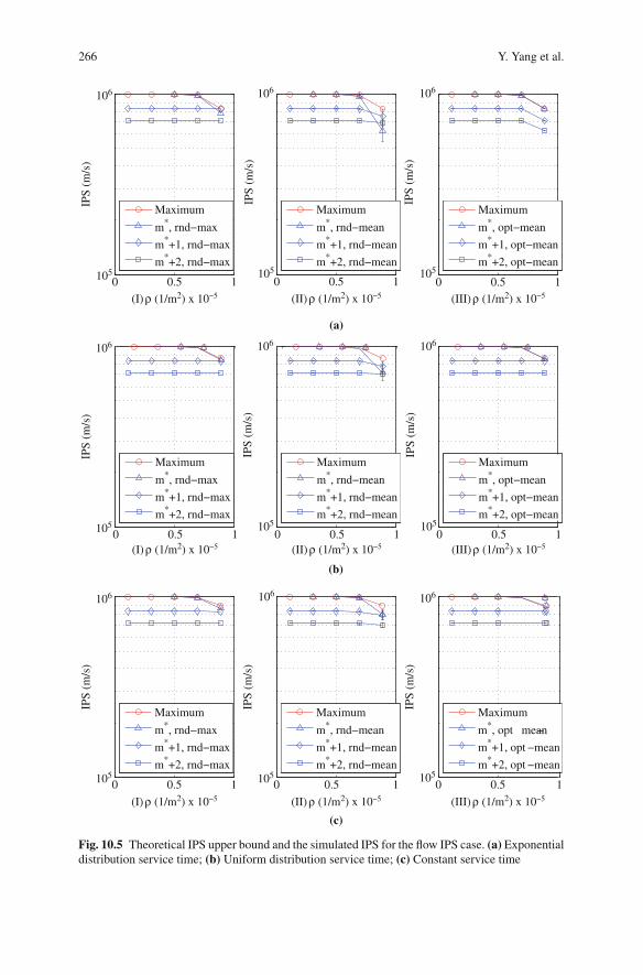
• Flow IPS CaseNext, we compare our theoretical IPS upper bound with the actual IPS computedfrom simulations in the flow IPS case. The simulation region is a square withedge length 10, 000 m. The PU transmitters are uniformly distributed within thesimulation region. The source–destination distance is 500 m. We simulate m∗-hop, m∗ + 1-hop, and m∗ + 2-hop SU paths, where m∗ is the optimal numberof relay nodes. For each path length, we generate 50 paths and for each path, wegenerate 50 PU transmitter distribution. For each of the setting, we measure thedelays for 20, 000 packet deliveries between the source and the destination. Inthe simulation, K = 20, rc = 110 m, τ0 = 0.1 ms, Tr

Ts= 2, and μ−1

P = 1 ms.Three possible PU service time distributions are simulated: exponential distri-bution, uniform distribution, and constant. Their simulation results are shown inFig. 10.5(a–c), respectively.

We perform two sets of simulations for each distribution. In the first set of simula-tions, we randomly position SU nodes as long as they maintain connectivity between


(a)

105

107

106

IPS

(m/s

)

IPS

(m/s

)

105

107

106

IPS

(m/s

)

Maximum1 hop, rnd−max2 hop, rnd−max3 hop, rnd−max

Maximum1 hop, rnd−mean2 hop, rnd−mean3 hop, rnd−mean

0 0.5 1 0 0.5 1 0 0.5 1

Maximum

d*, line−mean

0.8d*, line−mean1.2d*, line−mean

(I) ρ (1/m2) x 10−5 (II) ρ (1/m2) x 10−5 (III) ρ (1/m2) x 10−5

(b)

IPS

(m/s

)

IPS

(m/s

)

IPS

(m/s

)

0 0.5 1 0 0.5 1 0 0.5 1105

107

106

105

107

106

105

107

106


−

Maximum1 hop, rnd−max2 hop, rnd−max3 hop, rnd−max


Maximum

d*, line−mean0.8d*, line−mean1.2d*, line−mean

(c)

0 0.5 1

IPS

(m/s

)

IPS

(m/s

)

IPS

(m/s

)

0 0.5 1 0 0.5 1105

107

106

105

107

106

105

107

106




Maximumd*, line−mean0.8d*, line−mean1.2d*, line−mean

105

107

106

Fig. 10.4 Theoretical IPS upper bound and the simulated IPS for the network IPS case.(a) Exponential distribution service time; (b) Uniform distribution service time; (c) Constant ser-vice time

266 Y. Yang et al.

(a)

105

106IP

S (m

/s)

105

106

IPS

(m/s

)

105

106

IPS

(m/s

)

(b)

105

106

IPS

(m/s

)

105

106

IPS

(m/s

)

0 0.5 1105

106

IPS

(m/s

)

0 0.5 1

0 0.5 1

0 0.5 1 0 0.5 1 0 0.5 1

(I) ρ (1/m2) x 10−5

(I) ρ (1/m2) x 10−5

(I) ρ (1/m2) x 10−5

(III) ρ (1/m2) x 10−5

(III) ρ (1/m2) x 10−5

(III) ρ (1/m2) x 10−5(II) ρ (1/m2) x 10−5

(II) ρ (1/m2) x 10−5

(II) ρ (1/m2) x 10−5

1

(c)

0 0.5 1

106 106 106

IPS

(m/s

)

0 0.5 1

IPS

(m/s

)

0 0.5105105 105

IPS

(m/s

)

Maximum

m*, rnd−max

m*+1, rnd−max

m*+2, rnd−max

Maximum

m*, rnd−mean

m*+1, rnd−mean

m*+2, rnd−mean

Maximum

m*, opt−mean

m*+1, opt−mean

m*+2, opt−mean

Maximum

m*, rnd−max

m*+1, rnd−max

m*+2, rnd−max

Maximum

m*, rnd−mean

m*+1, rnd−mean

m*+2, rnd−mean

Maximum

m*, opt−mean

m*+1, opt−mean

m*+2, opt−mean

Maximum

m*, rnd−max

m*+1, rnd−max

m*+2, rnd−max

Maximum

m*, rnd−mean

m*+1, rnd−mean

m*+2, rnd−mean

−mean

−mean

−mean

Maximum

m*, opt

m*+1, opt

m*+2, opt

Fig. 10.5 Theoretical IPS upper bound and the simulated IPS for the flow IPS case. (a) Exponentialdistribution service time; (b) Uniform distribution service time; (c) Constant service time


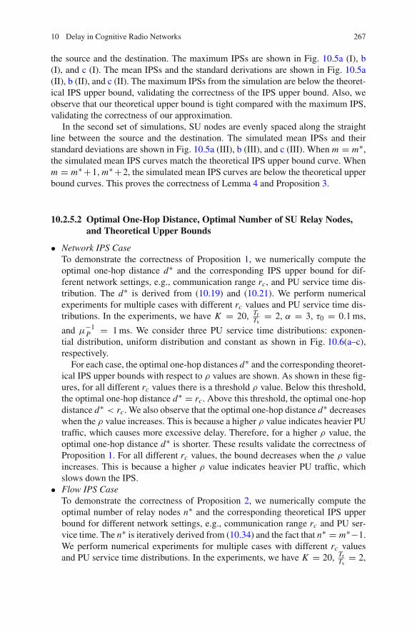
the source and the destination. The maximum IPSs are shown in Fig. 10.5a (I), b(I), and c (I). The mean IPSs and the standard derivations are shown in Fig. 10.5a(II), b (II), and c (II). The maximum IPSs from the simulation are below the theoret-ical IPS upper bound, validating the correctness of the IPS upper bound. Also, weobserve that our theoretical upper bound is tight compared with the maximum IPS,validating the correctness of our approximation.

In the second set of simulations, SU nodes are evenly spaced along the straightline between the source and the destination. The simulated mean IPSs and theirstandard deviations are shown in Fig. 10.5a (III), b (III), and c (III). When m = m∗,the simulated mean IPS curves match the theoretical IPS upper bound curve. Whenm = m∗+1,m∗+2, the simulated mean IPS curves are below the theoretical upperbound curves. This proves the correctness of Lemma 4 and Proposition 3.

10.2.5.2 Optimal One-Hop Distance, Optimal Number of SU Relay Nodes,and Theoretical Upper Bounds

• Network IPS CaseTo demonstrate the correctness of Proposition 1, we numerically compute theoptimal one-hop distance d∗ and the corresponding IPS upper bound for dif-ferent network settings, e.g., communication range rc, and PU service time dis-tribution. The d∗ is derived from (10.19) and (10.21). We perform numericalexperiments for multiple cases with different rc values and PU service time dis-tributions. In the experiments, we have K = 20, Tr

Ts= 2, α = 3, τ0 = 0.1 ms,

and μ−1P = 1 ms. We consider three PU service time distributions: exponen-

tial distribution, uniform distribution and constant as shown in Fig. 10.6(a–c),respectively.

For each case, the optimal one-hop distances d∗ and the corresponding theoret-ical IPS upper bounds with respect to ρ values are shown. As shown in these fig-ures, for all different rc values there is a threshold ρ value. Below this threshold,the optimal one-hop distance d∗ = rc. Above this threshold, the optimal one-hopdistance d∗ < rc. We also observe that the optimal one-hop distance d∗ decreaseswhen the ρ value increases. This is because a higher ρ value indicates heavier PUtraffic, which causes more excessive delay. Therefore, for a higher ρ value, theoptimal one-hop distance d∗ is shorter. These results validate the correctness ofProposition 1. For all different rc values, the bound decreases when the ρ valueincreases. This is because a higher ρ value indicates heavier PU traffic, whichslows down the IPS.

• Flow IPS CaseTo demonstrate the correctness of Proposition 2, we numerically compute theoptimal number of relay nodes n∗ and the corresponding theoretical IPS upperbound for different network settings, e.g., communication range rc and PU ser-vice time. The n∗ is iteratively derived from (10.34) and the fact that n∗ = m∗−1.We perform numerical experiments for multiple cases with different rc valuesand PU service time distributions. In the experiments, we have K = 20, Tr

Ts= 2,

268 Y. Yang et al.

0 0.5 1 1.5 2 2.5 3

x 10−5

50

100

150

d* (

m)

d* (

m)

0

(a)

(b)

0.5 1 1.5 2 2.5 3

x 10−5

106

107

105

106

107

105

ρ (1/m2)

Max

imum

IPS

(m

/s)

0 0.5 1 1.5 2 2.5 3

x 10−5

50

100

150

0 0.5 1 1.5 2 2.5 3

x 10−5ρ (1/m2)

Max

imum

IPS

(m

/s)

rc = 70 m

rc = 150 m

rc = 110 m

rc = 70 m

rc = 150 m

rc = 110 m

rc = 70 m

rc = 150 m

rc = 110 m

rc = 70 m

rc = 150 m

rc = 110 m

Fig. 10.6 Optimal one-hop distance d∗ and IPS upper bound for the network IPS case. (a) Expo-nential distribution service time; (b) Uniform distribution service time; (c) Constant service time

α = 3, τ0 = 0.1 ms, and μP = 1 ms. We consider three PU service time distri-butions: exponential distribution, uniform distribution, and constant as shown inFig. 10.7(a–c), respectively.

For each case, the optimal number of relay nodes n∗ and the corresponding the-oretical IPS upper bounds with respect to ρ values are shown. As shown in thesefigures, for each rc value there are threshold ρ values. Above these thresholds,


(c)

106

107

105

0 0.5 1 1.5 2 2.5 3

x 10−5

50

100

150

d* (

m)

0 0.5 1 1.5 2 2.5 3

x 10−5ρ (1/m2)

Max

imum

IPS

(m

/s)

rc = 70 m

rc = 150 m

rc = 110 m

rc = 70 m

rc = 150 m

rc = 110 m

Fig. 10.6 (continued)

(a)

0 0.5 1 1.5 2 2.5 3

0 0.5 1 1.5 2 2.5 3

10

20

30

40

n*M

axim

um I

PS (

m/s

)

x 10−5

x 10−5

105

106

107

ρ (1/m2)

rc = 110 m

rc = 70 m

rc = 150 m

rc = 110 m

rc = 70 m

rc = 150 m

Fig. 10.7 Optimal number of relay SU nodes n∗ and IPS upper bound for the flow IPS case.(a) Exponential distribution service time; (b) Uniform distribution service time; (c) Constant ser-vice time

270 Y. Yang et al.

105

106

107

(c)

0 0.5 1 1.5 2 2.5 3

x 10−5

10

20

30

40

n*

0 0.5 1 1.5 2 2.5 3

x 10−5ρ (1/m2)

Max

imum

IPS

(m

/s)

rc = 110 m

rc = 70 m

rc = 150 m

rc = 110 m

rc = 70 m

rc = 150 m

(b)

0 0.5 1 1.5 2 2.5 310

20

30

40

0 0.5 1 1.5 2 2.5 3

Max

imum

IPS

(m

/s)

x 10−5

x 10−5

ρ (1/m2)

rc = 110 m

rc = 70 m

rc = 150 m

rc = 110 m

rc = 70 m

rc = 150 m

n*

105

106

107

Fig. 10.7 (continued)

n∗ increments. We also observe that n∗ is a non-decreasing function of ρ. Thisis because when ρ is large, the IPS is mainly constrained by the interference fromPU traffic. A larger number of relay nodes results in a shorter one-hop distance anda shorter sensing range, rendering less interference from PU traffic. Therefore, n∗ isa non-decreasing function of ρ. These results validate the correctness of Proposition2. The general trends and underlying rationales are the same as that of the networkIPS case. The bounds are slightly below the bounds of the network IPS case. This


is because the source–destination distance is not necessarily a multiple of d∗ in thenetwork IPS case, which decreases the IPS.

10.3 Delay Analysis in Single-Hop Cognitive Radios Networks

As discussed in Section 10.2, the total delay of a flow is a combination of both infor-mation propagation delay and queueing delay. While Section 10.2 gives an analysisfor information propagation delay in multihop CRN, accurate analysis of queueingdelays in such networks is still an open problem due to the complex correlationsbetween packet loss, queue length, scheduling algorithms, and interference amongall the hops of a flow. However, in a single-hop CRN network, it is possible toprovide accurate analysis of the total delay that includes both information propa-gation delay and queueing delay with detailed consideration of many CRN designcharacteristics. In this section, we will provide such an analysis.

One design characteristic that we consider in CRN is channel aggregation. Usu-ally, licensed spectrum is divided into a number of discrete channels. As in theShannon’s theorem, channel capacity is proportional to channel width (bandwidth).Hence, efficient utilization of white spaces can be achieved by properly enablingeach SU to access multiple channels at a time [11]. This assembling of non-contiguous channels for communication is called channel aggregation as definedin IEEE 802.22 draft [12]. Technically, channel aggregation can be implementedbased on orthogonal frequency division multiplexing (OFDM) [13–15] or multipleradios [16]. Other design characteristics that are considered in our analysis includethe duration of each transmission attempt, the delay in channel sensing and channelswitching, and the handshake delay for channel negotiation among communicationpeers.

This section is organized as follows. First, we propose a new channel usagemodel to investigate the impact of both PU and SU behaviors on the availabilityof white spaces for channel aggregation. Unlike the ON-OFF process, this gen-eral model can capture a wider range of user behaviors. Next, we derive the delaycosts for performing channel aggregation under this model. User demands in bothfrequency and time domains are considered to evaluate the costs for making nego-tiation and renewing transmission. Further, an optimal channel aggregation strategyis defined in order to minimize the cumulative delay for transmitting data. Finally,numerical analysis and discrete-event simulation are used to illustrate and validateour model and the optimal channel aggregation strategy.

10.3.1 System Model

10.3.1.1 Basic Assumptions

A SU is assumed to be equipped with a dedicated radio for operating ondata channels in vacant licensed spectrum bands and another scanner radio for

272 Y. Yang et al.

sending/receiving control messages on a dedicated control channel in unlicensedspectrum band [17, 18]. In addition, the scanner radio is responsible for sensingthe licensed spectrum bands to discover spectrum white spaces, denoted as Wn ,in its sensing region Vn . Denoting F ={ f1, · · ·, fK } as the set of K channels inthe licensed spectrum bands, we have Wn ⊆F . For these data channels, each SUwith a b-channel bandwidth demand can assemble b channels at a time so as toform an aggregated channel A(b)={ f1′, · · ·, fb′ } ⊂F for data communication. Dueto limitations on radio design complexity, there exists a limit B on b such thatb≤ B. Usually, B is a small positive number. For example, in the IEEE 802.22standard, B = 3. In addition, if any two channels, say fl and fl+δ , are too farapart in F , they cannot be aggregated. This constraint for the channel separationis denoted as Δ (a.k.a. δ≤Δ). In other words, an A(b) can only be selected fromCl,Δ={ fl , · · ·, fl+Δ}⊂F , which is a set of candidate channels satisfying the Δconstraint.

Whenever a sender n tries to send data packets to its receiver n′, a negotiationbetween n and n′ via control channel is necessary for an agreement on the formingof the aggregated channel A(b). It is assumed that each SU does not have full knowl-edge of spectrum usage in its vicinity. Thus, multiple negotiation attempts betweenn and n′ may be needed to finalize A(b) that satisfy the Δ constraint.

Specifically, n should first sense a set of channels to find common white spacesin both Vn and Vn′ . As shown in the example in Fig. 10.8, first, n picks a spectrumrange Cl,Δ (e.g., C7,4 = { f7, f8, f9, f10} in the 1st attempt) that satisfies the Δ

constraint to sense. This leads to the discovery of the white space Tl,Δ= Cl,Δ ∩Wn

(e.g., T7,4 = {9} in 1st attempt). Then, n checks if |Tl,Δ| ≥ b = 2. If not the case(e.g., 1st attempt), we call it a blocking incident at the sender and n will pick anotherspectrum range Cl,Δ to sense for white spaces until finally it finds a white space Tl,Δ

that is larger than b. Then, n initiates a handshake with n′ to see if enough channelsin Tl,Δ is also available in n′ such that |Pl,Δ|= |Tl,Δ ∩Wn′ | ≥ b. If not true (e.g.,attempt 2nd), a blocking incident at the receiver happens and n is informed to go

Fig. 10.8 An example of negotiation and transmission between n and n′


Fig. 10.9 Channel usage model

over all the spectrum sensing and handshake steps again until finally a viable Pl,Δ

is found (e.g., attempt 3rd). Then, n′ selects an A(b)⊆Pl,Δ and replies to n. Then,a transmission S(b)={s1′, · · ·, sb′ } is initiated, which includes b parallel subflowswith a d-slot duration demand.

However, a successful negotiation does not mean a reliable transmission,attributed to the low priority of SU service. To overcome this, spectrum switching isemployed. Specifically, whenever a PU arrival to any fk ∈A(b) is detected, the pairof n and n′ needs to vacate the preempted fk immediately and then tries to renewthe corresponding sk on a backup channel fk′ ∈Bl,Δ, where Bl,Δ=Pl,Δ\A(b). Forease of presentation, such spectrum switching is divided into two steps: “outward”switching from fk and “inward” switching to fk′ . If |Bl,Δ| = 0, an interruption inci-dent occurs to the expelled sk . But all the other ongoing ones in S(b) may not beaffected as long as the independence of these parallel subflows is guaranteed [19].

10.3.1.2 Channel Usage Model

In a certain SU n’s vicinity, any channel fc ∈F may be occupied by an active PUor SU service for a period of time. As in Fig. 10.9, the average channel occupancyon such fc is modeled as a Markov chain, in which channel state transits on a slotbasis with a τ -second slot duration. Three groups of channel states are defined asfollows: (i) idle state (0,0), in which fc is a white space; (ii) PU service states(x ,0)’s, x ∈ {1, · · ·, X}, in which fc has been occupied by a PU service for x slots;(iii) SU service states (0,y)’s, y ∈ {1, . . .,Y }, in which fc has been occupied by aSU subflow for y slots. Both X and Y are large enough such that Pr[x > X ] andPr[y > Y ] are negligible. If there are multiple PU or SU services sharing fc, thestatistical data of the service with maximum duration can be applied.

The availability of white spaces is characterized by the steady-state probabili-ties of channel states, denoted by π(current state)’s, especially π(0,0) for idle state. To

derive them, the transition probabilities, denoted by ω(next state)(current state)’s, are obtained as

follows.

(1) First, state transitions from (0,0) and (0,y)’s to (1,0) represent a PU arrival tofc. Each transition from (0,y) to (1,0) also indicates an “outward” switching ofthe SU from fc. The transition probabilities are actually equal to the PU arrival

274 Y. Yang et al.

probability, denoted by λα , which further depends on the PU arrival processwith average arrival rate αn learnt in Vn . Namely, we have

ω(1,0)(0,0) = ω

(1,0)(0,y) = λα, y ∈ {1, . . .,Y } (10.38)

(2) Next, state transitions from (x ,0)’s to (0,0) and that among (x ,0)’s are definedby the distribution of PU service duration on fc. Note that any closed-formdistribution function is not necessarily required here. Instead, one can directlyinput the statistical distribution of service duration collected from a real networkto determine the following transition probabilities

⎧⎪⎨⎪⎩ω(0,0)(x,0) = Pr

[(x−1)τ < Spu ≤ xτ

], x ∈ {1, · · ·, X};

ω(x+1,0)(x,0) = 1−ω(0,0)(x,0), x ∈ {1, · · ·, X−1}

(10.39)

where Spu denotes the random variable of PU service duration.(3) In a similar way, state transitions from (0,y)’s to (0,0) and that among (0,y)’s

are defined by the distribution of SU service duration on fc, which can also begeneral. Hence, we have

⎧⎪⎨⎪⎩ω(0,0)(0,y) =

(1−ω(1,0)(0,y)

)Pr[(y−1)τ < Ssu ≤ yτ

], y ∈ {1, · · ·,Y };

ω(0,y+1)(0,y) = 1−ω(1,0)(0,y)−ω(0,0)(0,y), y ∈ {1, · · ·,Y−1}

(10.40)

where Ssu denotes the random variable of SU service duration.(4) State transition from (0,0) to (0,1) is triggered by a SU arrival. The SU arrival

probability, denoted by λβ , is determined by the SU arrival process with averagearrival rate βn learnt in Vn .

State transition from (0,0) to (0,y) where y > 1 is triggered by an “inward”switching to fc. Each transition from (0,0) to (0,y) indicates the case that a subflowsc′ switches to fc when it has last y-1 slots on another channel fc′ and has beenforced to leave fc′ due to the arrival of PU activities on fc′ . The subflow is renewedon fc starting from the yth slot.

To derive the state transition probability in the above two cases, we first derive theprobability that a certain subflow has successfully switched into fc, denoted by γ .Due to Δ constraints, only the 2·Δ channels excluding fc in Cc−Δ,2Δ can performan “inward” switching to fc. If there are u preempted channels and v idle channelsout of such 2·Δ channels, γ is equivalent to the probability that one of the u expelledsubflows successfully chooses fc out of the total v+1 idle channels for an “inward”switching. Here the worst case is analyzed, in which any incoming subflow neglectsthe idle channels that are not included in Cc−Δ,2Δ. Then, we have


γ =∑2Δu=1

∑2Δ−uv=0

(2Δ)!u!v!(2Δ−u−v)!

[λα

(∑Yy=1 π(0,y)

)]u (π(0,0)

)v·[1−λα

(∑Yy=1 π(0,y)

)−π(0,0)

]2Δ−u−vmin

{u

v+1 , 1} (10.41)

Given that a subflow, say sc′ , has switched into fc, we further derive ξ (0,y), theprobability that sc′ has finished (y–1) slots on fc′ . Assuming that the primary userarrival is independent of the secondary user activities, we have

ξ (0,y) =∑Yz=y Pr [(z−1)τ < Ssu ≤ zτ ] , y ∈ {2, . . .,Y } (10.42)

Using (10.4) and (10.5), we have the following transition probabilities

⎧⎪⎨⎪⎩ω(0,1)(0,0) =

(1−ω(1,0)(0,0)

)λβ;

ω(0,y)(0,0) =

(1−ω(1,0)(0,0)

)γ ξ(0,y), y ∈ {2, . . .,Y }

(10.43)

At last, we have the transition probability from (0,0) to itself

ω(0,0)(0,0) = 1−ω(1,0)(0,0)−

∑Yy=1 ω

(0,y)(0,0) (10.44)

10.3.2 Delay Analysis Under Channel Aggregation

Both the negotiation and the transmission between a sender n and its receiver n′can involve service failures and delay costs. In this section, we investigate the cor-responding service failure probabilities and model the delay costs for performingchannel aggregation under the influence of PU activity.

10.3.2.1 Delays in Negotiation Process

The efficiency of negotiation between n and n′ is restricted by the availability ofwhite spaces in both Vn and Vn′ . In general, the delays for making a successfulnegotiation include: (i) sensing delay T (b)

ss , which is the time required for sensingchannels at both n and n′; (ii) handshake delay T (b)

hs , which is the time requiredfor accessing control channel and making handshakes on it back and forth. In thefollowing, these delays in negotiation processes are analyzed.

Note that after each blocking incident caused by |Pl,Δ|< b, a new round of hand-shake needs to be started until the maximum limit of blocking incidents, denoted asN̂bl, is reached. Hence, negotiation delays are related to the number of blockingincidents during a negotiation process.

To analyze the number of blocking incidents, note that the blocking probability,denoted as θ(b), can be computed as:

276 Y. Yang et al.

θ(b) =∑b−1v=0

(Δ+1v

) (π(0,0)

)v (1− π(0,0))(Δ+1)−v (10.45)

where π0,0 is the probability that a channel is idle in the joint sensing range of apair of SUs n and n′ (a.k.a. Vn ∪ Vn′ ). The PU and SU’s arrival rates in Vn ∪ Vn′ canbe derived as αn,n′ = cn,n′ ·αn and βn,n′ = cn,n′ ·βn respectively, where cn,n′ denotesthe correlation factor between the arrival rate in Vn and the arrival rate in Vn ∪ Vn′ .Replacing αn and βn with αn,n′ and βn,n′ in the channel model in Section 10.3.1.2,π(0,0) in (10.45) can be computed.

Assume that an entire negotiation process is considered failed when the numberof blocking incident reaches the threshold N̂bl with no success. Then, the negotiationfailure probability, denoted as ε(b), can be expressed as:

ε(b) = 1−∑N̂blr=0

(θ(b)

)r (1−θ(b)) (10.46)

With (10.45) and (10.46), the expected number of blocking incidents in a suc-cessful negotiation process becomes:

N (b)bl = 1

1−ε(b)∑N̂bl

r=0

(θ(b)

)r (1−θ(b)) r (10.47)

Note that not every blocking incident costs the delay of a handshake since ninitiates a handshake only when |Tl,Δ| ≥ b. Therefore, we also need to obtain theblocking probability due to |Tl,Δ|< b, which is denoted as θ̃ (b). The same formulain (10.45) can be used to compute θ̃ (b) in a similar way as θ(b). The only differenceis that the π(0,0) in the expression of θ̃ (b) is computed using αn and βn , which arethe PU and SU arrival rates in Vn . With θ̃ (b) computed, the expected number ofhandshake attempts for a successful negotiation can be computed as:

N (b)hs = N (b)

bl

(1− θ̃ (b)

θ (b)

)+1 (10.48)

where 1−θ̃ (b)/θ(b) denotes the probability that |Tl,Δ| ≥ b but |Pl,Δ|< b.Assuming that sequential sensing is used [20, 21], based on (10.48) and (10.47),

we can compute the sensing delay T (b)ss as follows. In sequential sensing, whenever

a new Cl,Δ is chosen, n needs to sense the channels in it to keep Tl,Δ fresh, while n′senses the channels in Tl,Δ to complete the entire negotiation. Hence, we can get:

T (b)ss = N (b)

hs

[∑Δ+1v=b

(Δ+1v

) (π(0,0)

)v (1−π(0,0))(Δ+1)−vv]τss +

(N (b)

bl +1)(Δ+1) τss,

(10.49)

where τss denotes the average time for sensing one channel, and π(0,0) is computedusing αn and βn . We can also compute the handshake delay as:

T (b)hs = N (b)

hs (τma+τrt) , (10.50)


where τma denotes the average time for accessing control channel, which would begiven by classic analytical models [22]; and τrt denotes the round-trip time for onehandshake.

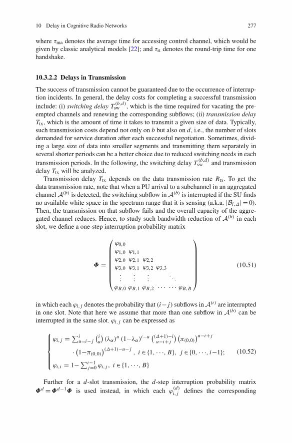
10.3.2.2 Delays in Transmission

The success of transmission cannot be guaranteed due to the occurrence of interrup-tion incidents. In general, the delay costs for completing a successful transmissioninclude: (i) switching delay T (b,d)

sw , which is the time required for vacating the pre-empted channels and renewing the corresponding subflows; (ii) transmission delayTtx, which is the amount of time it takes to transmit a given size of data. Typically,such transmission costs depend not only on b but also on d, i.e., the number of slotsdemanded for service duration after each successful negotiation. Sometimes, divid-ing a large size of data into smaller segments and transmitting them separately inseveral shorter periods can be a better choice due to reduced switching needs in eachtransmission periods. In the following, the switching delay T (b,d)

sw and transmissiondelay Ttx will be analyzed.

Transmission delay Ttx depends on the data transmission rate Rtx. To get thedata transmission rate, note that when a PU arrival to a subchannel in an aggregatedchannel A(b) is detected, the switching subflow in A(b) is interrupted if the SU findsno available white space in the spectrum range that it is sensing (a.k.a. |Bl,Δ| = 0).Then, the transmission on that subflow fails and the overall capacity of the aggre-gated channel reduces. Hence, to study such bandwidth reduction of A(b) in eachslot, we define a one-step interruption probability matrix

Φ =

⎛⎜⎜⎜⎜⎜⎜⎜⎝

ϕ0,0ϕ1,0 ϕ1,1ϕ2,0 ϕ2,1 ϕ2,2ϕ3,0 ϕ3,1 ϕ3,2 ϕ3,3...

......

. . .

ϕB,0 ϕB,1 ϕB,2 · · · · · · ϕB,B

⎞⎟⎟⎟⎟⎟⎟⎟⎠

(10.51)

in which each ϕi, j denotes the probability that (i− j) subflows in A(i) are interruptedin one slot. Note that here we assume that more than one subflow in A(b) can beinterrupted in the same slot. ϕi, j can be expressed as

⎧⎪⎪⎪⎨⎪⎪⎪⎩ϕi, j =∑i

u=i− j

( iu

)(λα)

u (1−λα)i−u ((Δ+1)−iu−i+ j

) (π(0,0)

)u−i+ j

· (1−π(0,0))(Δ+1)−u− j, i ∈ {1, · · ·, B}, j ∈ {0, · · ·, i−1};

ϕi,i = 1−∑i−1j=0 ϕi, j , i ∈ {1, · · ·, B}

(10.52)

Further for a d-slot transmission, the d-step interruption probability matrixΦd =Φd−1Φ is used instead, in which each ϕ

(d)i, j defines the corresponding

278 Y. Yang et al.

bandwidth reduction of A(i) within d slots. Note that ϕ(d)b,0 is the complete trans-

mission failure probability, where all the subflows of A(b) are interrupted. With Φd ,the average transmission rate for a transmission attempt can be expressed as

Rtx =⎛⎝ b∑

j=0

ϕ(d)b, j R jdτ

⎞⎠ (10.53)

where R denotes the bit rate on one channel and τ is the duration of a time slot.Next, the switching delay T (b,d)

sw for a successful d-slot subflow is analyzed.Given that there is no interruption, let χ(b) be the probability that a switching oper-ation succeeds in one slot. We have

χ(b) = λα

[1−(1−π(0,0))(Δ+1)−b

]1−λα(1−π(0,0))(Δ+1)−b

(10.54)

in which π(0,0) is computed using αn,n′ and βn,n′ . Within d slots, the expected num-ber of switching operations is

N (b,d)sw =∑d

z=0

(dz

) (χ(b)

)z (1−χ(b))d−z

z (10.55)

Accordingly, for a successful d-slot subflow, we have

T (b,d)sw = N (b,d)

sw τsw (10.56)

where τsw denotes the time required for one switching operation. The sensing timefor locating backup channels can be negligible due to the simultaneous operationsof the cognitive radio and scanning radio.

10.3.3 Optimal Bandwidth Duration Decision

Based on the derived negotiation and transmission costs for performing channelaggregation, in this section, we further define an optimal channel aggregation strat-egy that minimizes the cumulative delay costs.

10.3.3.1 Cumulative Delay

As shown above, the delay costs for channel aggregation are closely related to thevalues of b and d, i.e., the user demands on aggregated bandwidth and service dura-tion. On one hand, the choice of b should consider the trade-off between channelcapacity and blocking (interruption) probability during a negotiation (transmission).More white spaces are needed to meet a higher requirement of b. On the other hand,the choice of d should consider the trade-off between negotiation overhead andinterruption probability during a transmission. With certain data to transmit, one can


choose to divide the entire data into d-slot segments. A larger value of d results infewer data segments and thus fewer negotiation operations. However, there may bemore spectrum resources wasted due to higher interruption probability. Therefore,there exists an optimal combination of b and d to achieve optimal efficiency ofchannel aggregation.

The optimal efficiency is represented by a metric named cumulative delay, whichis the total amount of time needed for transmitting a M-bit size data. Note that theaverage amount of data that can be successfully transmitted by each attempt is

M̃ (b,d) = (1−ε(b)) Rtx (10.57)

In addition, an attempt can meet three cases: (i) fails at negotiation stage, (ii) suc-ceeds in negotiation but fails at transmission; and (iii) succeeds in both negotiationand transmission. The average cumulative delay, denoted as T (b,d)

cm , must accountfor all the cases. Hence,

T (b,d)cm = M

M̃(b,d)

{ε(b)

(T̂ (b)

ss +T̂ (b)hs

)+ (

1−ε(b)) [T (b)ss +T (b)

hs

+ϕ(d)b,0

(T

(b, d

2

)sw + d

2 τ

)+(

1−ϕ(d)b,0

) (T (b,d)

sw +dτ)]} (10.58)

in which T̂ (b)ss and T̂ (b)

hs are computed by replacing the expected negotiation times

N (b)bl with negotiation failure threshold N̂bl in (10.49) and (10.50), respectively, and

the expected duration of failed service related to ϕ(d)b,0 is assumed to be d/2.

10.3.3.2 Optimal Channel Aggregation Strategy

A channel aggregation strategy (b, d) is defined as the combination of both band-width and duration demands. The objective is to find the optimal (b∗, d∗) that min-imizes T (b,d)

cm :

(b∗, d∗) = arg min(b,d)∈G

T (b,d)cm (10.59)

It is not hard to find (b∗, d∗) by searching the finite set of all possible (b, d)’s.Note that in CR networks, both PU and SU behaviors that affect the availability ofwhite spaces are stochastic. Hence, the optimal channel aggregation strategy definedin (10.59) is actually optimal in the sense of average performance.

280 Y. Yang et al.

10.3.4 Numerical Analysis and Simulation Results

To illustrate and validate the analytical results, figures that are derived from numer-ical analysis and discrete-event simulation of a few of our analytical results areshown in this section, including the negotiation failure probability ε(b) in (10.46),the transmission failure probability ϕ(d)b,0 defined in Section 10.3.2.2, and the cumu-

lative delay T (b,d)cm in (10.58). These figures will show the impact of PU activity

and channel aggregation strategy on the efficiency of negotiation and transmissionbetween secondary users.

In the numerical analysis, a pair of PU sender and receiver, n and n′, in a dis-tributed CR network is considered. Poisson PU arrival process is assumed in bothVn and Vn′ areas. The distribution of PU service duration is set according to thestatistical distribution of call duration collected from a real cellular network [5]. Asfor SU behavior, Poisson SU arrival process and random SU service duration areassumed. Note that the choice of service duration for the pair of n and n′ is a part oftheir optimal decision, but we fix the patterns of SU activity in the background. Theconstant parameters are set as follows: K = 50; B = 3; βn = 0.02 user/s; cn,n′ = 1.5;E[Y ]= 3 s; τ = 10 ms; τss = 10 ms [18, 21]; τr t = 200 ms; τsw = 600 ms [20];N̂bl = 5; M = 50 Mb; R= 5 Mb/s. The others are viewed as variables.

10.3.4.1 Illustration of Negotiation Failure Probability

As in (10.46), ε(b) defined for negotiation failure which characterizes the repeatedblocking incidents caused by lack of enough common white space at n and n′ (a.k.a.|Pl,Δ|< b). The impact of αn and Δ on ε(b) with fixed transmission duration ofd·τ = 3 s is plotted in Fig. 10.10. Generally, the numerical results (marked as “ana”)and simulation results (marked as “sim”) match well with each other under the samesettings. It can be seen that with a higher demand on b or a drop in the availabilityof white spaces, ε(b) increases. In addition, a relaxation of the hardware limitationon Δ offers more candidate channels and thus lowers ε(b).

Fig. 10.10 Negotiation failure probability vs. PU arrival rate: (i) Δ = 10 (left); (ii) Δ = 20 (right)


Fig. 10.11 Transmission failure probability vs. duration demand: (i) Δ= 10 (left); (ii) Δ= 20(right)

10.3.4.2 Illustration of Transmission Failure Probability

The impact of transmission duration d on transmission failure probability ϕ(d)b,0 is

shown at Fig. 10.11, where the PU traffic arrival rate is fixed at αn = 0.1 user/s.Defined in Section 10.3.2.2, ϕ(d)b,0 is the probability that all subflows of an aggregatedchannel are interrupted halfway during a transmission by PUs. Clearly, with longertransmission duration dτ or a smaller channel separation constraint Δ, the ϕ

(d)b,0

increases. Interestingly, unlike negotiation failure probability ε(b), a larger transmis-sion duration b actually reduces transmission failure probability ϕ

(d)b,0. Intuitively,

this is because the transmission consisting of more subflows would tolerant moreinterruption incidents. Hence, a trade-off obviously exists among the negotiationfailure probability and transmission failure probability to achieve the overall optimaltransmission strategy.

10.3.4.3 Illustration of Cumulative Delay

For the transmission of M-bit data, the related cumulative delay T (b,d)cm has been

chosen as our objective function as in (10.58). In Figs. 10.12 and 10.13, the impactof αn and (b, d) on T (b,d)

cm is plotted, respectively. It can be seen that T (b,d)cm rises

rapidly with the increase of αn due to the increase of ε(b) and ϕ(d)b,0 in such cases. A

larger channel separation constraint Δ lowers T (b,d)cm . To achieve the lowest T (b,d)

cm ,the optimal channel aggregation strategy (b∗, d∗) is evaluated under different set-tings in Fig. 10.13. The marked point that represents the optimal decision variessignificantly with the availability of white spaces. Obviously, when there are plentyof white spaces as in Fig. 10.13-i, larger b and d are the optimal solution to achievethe highest utilization of licensed spectrum. Note that the range of d differs fordifferent values of b for transmitting the same size of data. However, if there arefew white spaces as in Fig. 10.13-iii, both b and d should be low to avoid the hugecosts for repeated negotiation and transmission attempt.

282 Y. Yang et al.

Fig. 10.12 Cumulative delay (in log scale) vs. PU arrival rate: (i) Δ= 10 (left); (ii) Δ= 20 (right)

Fig. 10.13 Cumulative delay vs. channel aggregation strategy: (i) αn = 0.01 user/s (left);(ii) αn = 0.1 user/s (middle); (iii) αn = 0.16 user/s (right)

10.4 Summary

In this section, we analyzed the delay for both multihop and single-hop CRN.For multihop CRN, we derive the IPS upper bound under two cases: the network

IPS and the flow IPS. In the network IPS case, we discover that the network IPSupper bound is related to a threshold value of the PU activity level. Below thethreshold, the IPS upper bound is achieved when the one-hop distance equals thecommunication range of cognitive radios. Above the threshold, the upper boundspeed is achieved when using an optimal one-hop distance which is less than thecommunication range. We design efficient numerical methods to compute the opti-mal one-hop distance and the corresponding IPS upper bound. In the flow IPS case,we discover that the IPS upper bound is achieved when an optimal number of SUrelay nodes are evenly spaced on the straight line between the source node and thedestination node. The optimal number of relay nodes shows a stair-like incrementaltrend, when the PU activity level increases. We design multiple numerical methodsto compute the optimal number of SU relay nodes. The simulation and numericalresults prove the correctness of our analysis.

For single-hop CRN, we have studied the delay under considerations of vari-ous practical constraints and costs. A new channel usage model based on generalassumptions is introduced to investigate the negotiation and transmission costs for


utilizing channel aggregation under the influence of PU activity. We have found thatuser demands on both aggregated bandwidth and service duration affect the delayperformance. Hence, an optimal channel aggregation strategy has been defined andvalidated to achieve the lowest delay for data transmission.

Acknowledgments This work was supported in part by the US National Science Foundationunder grant CNS-0831865 and the Institute for Critical Technology and Applied Science (ICTAS)of Virginia Tech.

References

1. Y. Xu and W. Wang, “The speed of information propagation in large wireless networks,” inProc. of IEEE INFOCOM, Phoenix, AZ, 2008.

2. R. Zheng, “Information dissemination in power-constrained wireless networks,” in Proc. ofIEEE INFOCOM, Barcelona, Catalunya, Spain, 2006.

3. P. Jacquet, B. Mans, P. Muhlethaler, and G. Rodolakis, “Opportunistic routing in wirelessad hoc networks: Upper bounds for the packet propagation speed,” in Proc. of IEEE MASS,Atlanta, Georgia, USA, 2008.

4. P. Jacquet, B. Mans, and G. Rodolakis, “Information propagation speed in mobile and delaytolerant networks,” in Proc. of IEEE INFOCOM, Rio de Janeiro, Brazil, 2009.

5. D. Willkomm, S. Machiraju, J. Bolot, and A. Wolisz, “Primary user behavior in cellularnetworks and implications for dynamic spectrum access,” IEEE Communications Magazine,vol. 47, pp. 88–95, 2009.

6. P. Popovski, H. Yomo, K. Nishimori, R. D. Taranto, and R. Prasad, “Opportunistic interferencecancellation in cognitive radio systems,” in Proc. of IEEE DySPAN, Dublin, Ireland, 2007.

7. R. Zhang and Y.-C. Liang, “Exploiting hidden power-feedback loops for cognitive radio,” inProc. of IEEE DySPAN, Chicago, Illinois, 2008.

8. G. Zhao, G. Y. Li, and C. Yang, “Proactive detection of spectrum opportunities in primary sys-tems with power control,” IEEE Transactions on Wireless Communications, vol. 8, pp. 4815–4823, 2009.

9. G. Bolch, S. Greiner, H. de Meer, K. S. Trivedi, H. de Meer, and K. S. Trivedi, QueueingNetworks and Markov Chains: Modeling and Performance Evaluation With Computer ScienceApplications. Wiley-Interscience, Wiley, 2006.

10. C. Han and Y. Yang, “Information propagation speed in cognitive radio networks: Networkand flow analysis,” Virginia Tech, Tech. Rep., 2010.

11. R. Chandra, R. Mahajan, T. Moscibroda, R. Raghavendra, and P. Bahl, “A Case for AdaptingChannel Width in Wireless Networks,” in Proc. ACM SIGCOMM’08, Seattle, WA, Aug. 2008.

12. IEEE 802.22 WG, “IEEE P802.22/D0.1 Draft Standard for Wireless Regional Area NetworksPart 22: Cognitive Wireless RAN Medium Access Control (MAC) and Physical Layer (PHY)Specifications: Policies and Procedures for Operation in TV Bands,” IEEE Standard, May2006.

13. S. Haykin, “Cognitive Radio: Brain-Empowered Wireless Communications,” IEEE Journalon Selected Areas in Communications, Vol. 23, No. 2, pp. 201–220, Feb. 2005.

14. H. Kim, and K. G. Shin, “Efficient Discovery of Spectrum Opportunities with MAC-LayerSensing in Cognitive Radio Networks,” IEEE Transactions on Mobile Computing, Vol. 7,No. 5, pp. 533–545, May 2008.

15. F. Huang, W. Wang, H. Luo, G. Yu, and Z. Zhang, “Prediction-Based Spectrum Aggrega-tion with Hardware Limitation in Cognitive Radio Networks,” in Proc. IEEE VTC’10-Spring,Taipei, Taiwan, May 2010.

284 Y. Yang et al.

16. P. Bahl, A. Adya, J. Padhye, and A. Wolman, “Reconsidering Wireless Systems with MultipleRadios,” ACM SIGCOMM Comp. Comm. Rev., Vol. 34, No. 5, pp. 39–46, Oct. 2004.

17. Y. Yuan, P. Bahl, R. Chandra, P. Chou, J. Ferrell, T. Moscibroda, S. Narlanka, and Y. Wu,“KNOWS: Kognitiv Networking Over White Spaces,” in Proc. IEEE DySPAN’07, Dublin,Ireland, Apr. 2007.

18. Y. Yuan, P. Bahl, R. Chandra, T. Moscibroda, and Y. Wu, “Allocating Dynamic Time-SpectrumBlocks in Cognitive Radio Networks,” in Proc. ACM MobiHoc’07, Montreal, QC, Canada,Sep. 2007.

19. J. Lee, and J. So, “Analysis of Cognitive Radio Networks with Channel Aggregation,” in Proc.IEEE WCNC’10, Sydney, Australia, Apr. 2010.

20. D. Xu, E. Jung, and X. Liu, “Optimal Bandwidth Selection in Multi-Channel Cognitive RadioNetworks: How Much Is Too Much?,” in Proc. IEEE DySPAN’08, Chicago, Illinois, Oct. 2008.

21. T. Shu, and M. Krunz, “Throughput-Efficient Sequential Channel Sensing and Probing inCognitive Radio Networks under Sensing Errors,” in Proc. ACM MobiCom’09, Beijing, China,Sep. 2009.

22. G. Bianchi, “Performance Analysis of IEEE 802.11 Distributed Coordination Function,” IEEEJournal on Selected Areas in Communications, Vol. 18, No. 3, pp. 535–547, Mar. 2000.

cognitive radio mobile ad hoc networks || delay in cognitive radio networks

Documents