coast information team - british columbia · coast information team ... five scenarios are analyzed...
TRANSCRIPT

Coast Information Team
c/o Cortex Consultants Inc., 3A–1218 Langley St. Victoria, BC, V8W 1W2 Tel: 250-360-1492 / Fax: 250-360-1493 / Email: [email protected]
September 16, 2004
The Coast Information Team is pleased to deliver the final version of the CIT Economic Gain Spatial Analysis–Timber for the CIT Region (August 2004).
The Coast Information Team (CIT) was established to provide independent information for the central and north coasts of British Columbia and Haida Gwaii/Queen Charlotte Islands using the best available scientific, technical, traditional and local knowledge. The CIT was established by the Provincial Government of British Columbia, First Nations, environmental groups, the forest industry, and communities. It was led by a management committee consisting of representatives of these bodies; and was funded by the Provincial Government, the environmental groups and forest products companies, and the Federal Government of Canada. The technical team comprised nine project teams consisting of scientists, practitioners, and traditional and local experts. CIT information and analyses, which include this CIT Economic Gain Spatial Analysis–Timber for the CIT Region, are intended to assist First Nations and the three sub-regional planning processes to make decisions that will achieve ecosystem-based management (as per the April 4th 2001 Coastal First Nations—Government Protocol and the CCLRMP Interim Agreement).
In keeping with the CIT’s commitment to transparency and highly credible independent analysis, an earlier version of this document, the CIT Economic Gain Spatial Analysis–Timber for the Central Coast Region, underwent an internal peer review and the CIT’s independent peer review process chaired by University of Victoria Professor Rod Dobell. Peer reviews of the draft document and the authors’ response are found at http://citbc.org/abopeer-comm.html. The final document reflects changes made by the authors to address peer review comments.
We encourage all stakeholders involved in land and resource management decision-making in the CIT area to use the information and recommendations/conclusions of the CIT Economic Gain Spatial Analysis–Timber for the CIT Region in conjunction with other CIT products as they seek to implement EBM and develop EBM Land Use Plans. We are confident that the suite of CIT products provides valuable information and guidance on the key tenets of EBM: maintaining ecosystem integrity and improving human wellbeing.
Sincerely,
Robert Prescott-Allen, Executive Director on behalf of the CIT Management Committee: Ken Baker, Art Sterritt, Dallas Smith, Jody Holmes, Corby Lamb Graem Wells, Gary Reay, Hans Granander, Tom Green, Bill Beldessi
Page 1

Coast Information Team
EGSA-Timber Ltr Transmittal_Sept04 Page 2

Coast Information Team
Economic Gain Spatial Analysis – Timber
CIT Region
Prepared by:
Doug Williams, Ph.D.
Mike Buell, B.S.F. Cortex Consultants Inc.
August 2004

Coast Information Team
EGSA Timber – CIT Central Coast Region August 2004
Page ii
Acknowledgements
The authors are grateful for the advice and contributions of many colleagues. John Sunde and Dan Sirk (Ministry of Sustainable Resource Management) developed the forest cover database. Jim Brown (Ministry of Forests [MOF]) provided background and insight on the Woodshed Model for the Central Coast Region. Dean Daly (Lynx Forestry Consultants) explained the North Coast woodshed studies and provided an analysis of potential linkages between this study and North Coast woodshed study. Laura Bolster (MOF) provided feedback on this study’s implementation of a North Coast timber supply model. Ed Gin (Cortex Consultants, Inc.) developed the coefficients for employment measures and revenue shares, with the guidance of Sinclair Tedder (MOF). Ed also developed the maps of inputs and value indicators by landscape. Rachel Holt (Veridian Consulting) clarified the data linkage between this project and the ecosystem risk analysis project underway on the same landbase. Jody Holmes (CIT Management Committee), Glenn Dunsworth (Weyerhaeuser), and Steven Northway (Weyerhaeuser) provided initial direction on the development of the ecosystem-based management scenarios. Allen Banner (MOF) provided estimates of the percentage area of ecosystems with red- and blue-listed species, and Karen Price provided estimates of the proportion of old forest expected under natural disturbance regimes. Glenn Sutherland (Cortex Consultants, Inc.) translated much of the advice on ecological matters acknowledged above into terms understandable by the authors.
We are also grateful to the two external reviewers, John Nelson and Jim Johnson, and to an internal reviewer, Tom Green (CIT Management Committee), for their insights and advice.

Coast Information Team
EGSA Timber – CIT Central Coast Region August 2004
Page iii
Executive Summary
This report presents the methods and results of the Economic Gain Spatial Analysis—Timber (EGSA-Timber) project for the Coast Information Team (CIT) Study Area of British Columbia This study was undertaken on the three subregions of the study area—the Central Coast, North Coast and Haida Gwaii /the Queen Charlotte Islands.
The objective of EGSA-Timber is to assign values derived from the harvesting and sale of timber to landscape units and to summarize these values at the subregion level for alternative management scenarios.
The general approach to assigning timber values to forest land that is employed in this study is to (1) develop a forest-level model that forecasts timber production and tracks changes in the landbase according to specified management objectives, and (2) use this model to generate time series of indicators of timber value attributable to each site under various scenarios of alternative management assumptions and objectives.
Five scenarios are analyzed for each CIT subregion in this study—a composite of the TSR Base Case scenarios of the constituent management units (TSAs and TFLs), a Financial Efficiency scenario that assumes base case management but maximizes the discounted cash flow from harvesting, and three scenarios applying Ecosystem-based Management Planning Handbook (EBMPH; CIT 2004) assumptions. The EBMPH scenarios all allow up to (i.e., ≤) low environmental risk at the subregional level and intermediate risk at the landscape level. The North Coast and Haida Gwaii scenarios allow high environmental risk at the watershed level; watershed level risk was not modelled for the Central Coast subregion as the appropriate watershed coverage was not included in the study’s landbase dataset. The three EBMPH scenarios analyzed for each region differ in that they allow low, intermediate, and high levels of risk at the stand level.
These scenarios are not meant to represent actual policy options that might be implemented. They are analyzed with the intention of bounding the set of feasible policies and providing sufficient information to allow one to infer the effects on values derived from timber harvesting from subsequent intermediate policies that may be implemented. The results are not intended for business planning or harvest scheduling purposes. Readers should be aware that the EGSA Timber model incorporates many sources of uncertainty—including, among others, questionable resource data, approximations to the EBMPH policies, and assumptions about future log prices
All scenarios other than the base case are implemented with an “even-flow” policy that ensures that the rate of harvest is constant. The even-flow harvest schedule was implemented in order to separate the impacts of the alternative management scenarios (FE and EBMPH) from the effects of complex flow policies such as the Ministry of Forests would normally apply in a TSR timber supply analysis. Flow policies that allow a gradual reduction in timber supply to a long-term harvest level would mitigate the short-term impacts of EBMPH and we expect that subsequent studies will explore such policies to determine feasible transitions from current harvest levels to EBMPH-based harvest levels.
The indicators of timber value calculated for each landscape and summed for the three CIT regions are summarized in Table ES.3. The results for the Central Coast subregion were calculated without a price trend. The results for the North Coast and Haida Gwaii subregions

Coast Information Team
EGSA Timber – CIT Central Coast Region August 2004
Page iv
were calculated with a price trend, but the effects of the trend have been removed in Table ES-1. Both formats (trended and not trended) are presented in the main report.
The forecast harvest levels associated with the composite TSR Base Case do not reflect reductions in the allowable annual cut (AAC) implemented since the most recent TSR in anticipation of landbase reductions, nor do they reflect reductions in harvest rates in response to poor market conditions.
Employment (direct) measures and employment income are determined from harvest volume. Net revenue is conversion return (revenue at market minus delivered wood cost), where delivered wood cost is determined independently from employment income. Stumpage is calculated as the residual after an allowance for profit and risk (12% of delivered wood costs) is subtracted from the net revenue. Note that all of the scenarios were evaluated with top-of-the-cycle prices and, therefore, revenue measures are best interpreted as indices rather than estimates of actual values.
These indicators were calculated for each landscape, and subsequently mapped onto the productive forest landbase. Two key inputs to this study, the forest resource and wood cost data, are also mapped on the productive forest landbase. These maps are available from the CIT Web site: http://www.citbc.org/anaecon.html .
The long-term impact on harvest levels (relative to the TSR Base Case) of implementing the intermediate stand-level risk scenario is large—a reduction of 41% from the TSR harvest level on the Central Coast, 52% on the North Coast, and 73% on Haida Gwaii. However, note that the impact on average net revenue is much smaller.
Table ES.1 Summary of indicators of timber value, CIT Study Area.
Central Coast LRMP AreaTSR Base
Case Financial
EfficiencyHigh Risk
Intermediate Risk
Low Risk
Short Term (20 year)
Harvest Volume ('000 m3/year) 3,871 3,054 2,824 1,884 1,038Employment - FTEs annual (LRMP) 1,027 810 717 476 258Employment - FTEs annual (BC) 3,841 2,944 2,752 1,836 1,017Employment Income (‘000 $/year) 48,615 38,328 33,807 22,486 12,188
Gross revenue ($/m3) 117.20 143.99 131.13 131.74 128.64 Delivered Wood Cost ($/m3) 88.35 79.27 83.85 86.68 90.56 Net Revenue ($/m3) 28.85 64.72 47.28 45.07 38.08 Rothery Stumpage ($/m3) 18.25 55.20 37.22 34.66 27.22 Profit Allowance to Enterprise ($/m3) 10.60 9.51 10.06 10.40 10.87
Long Term (200 years)
Harvest Volume ('000 m3/year) 3,214 3,054 2,824 1,884 1,038Employment - FTEs annual (LRMP) 842 802 739 493 271Employment - FTEs annual (BC) 3,111 2,951 2,731 1,821 1,003Employment Income ‘000 ($/year) 39,899 38,039 35,017 23,365 12,876
Gross Revenue ($/m3) 100.87 148.87 146.67 146.36 146.38Delivered Wood Cost ($/m3) 81.71 77.87 78.29 79.30 80.15Net Revenue ($/m3) 19.16 71.01 68.38 67.06 66.23Rothery Stumpage ($/m3) 9.36 61.66 58.98 57.55 56.61Profit Allowance to Enterprise ($/m3) 9.80 9.34 9.40 9.52 9.62
Net present value ('000 000 $) 2,033 3,707 2,148 1,761 895
Ecosystem Based Management

Coast Information Team
EGSA Timber – CIT Central Coast Region August 2004
Page v
Table ES.1 continued
CIT North Coast RegionTSR Base
Case Financial
EfficiencyHigh Risk
Intermediate Risk
Low Risk
Short Term (20 year)
Harvest Volume ('000 m3/year) 647 485 412 266 145Employment - FTEs annual (LRMP) 260 195 165 107 58Employment - FTEs annual (BC) 400 300 254 164 89Employment Income (‘000 $/year) 10,234 7,672 6,513 4,213 2,292
Gross revenue ($/m3) 125.95 174.76 135.03 135.63 136.11 Delivered Wood Cost ($/m3) 98.58 83.89 87.20 88.61 98.70 Net Revenue ($/m3) 27.38 90.86 47.83 47.02 37.41 Rothery Stumpage ($/m3) 15.55 80.80 37.36 36.39 25.57 Profit Allowance to Enterprise ($/m3) 11.83 10.07 10.46 10.63 11.84
Long Term (200 years)
Harvest Volume ('000 m3/year) 554 485 412 266 145Employment - FTEs annual (LRMP) 218 195 165 107 58Employment - FTEs annual (BC) 340 300 254 164 89Employment Income ‘000 ($/year) 8,795 7,672 6,513 4,213 2,292
Gross revenue ($/m3) 129.98 136.81 136.43 136.44 137.85Delivered Wood Cost ($/m3) 98.29 90.28 90.60 91.24 97.32Net Revenue ($/m3) 31.69 46.52 45.83 45.20 40.54Rothery Stumpage ($/m3) 19.89 35.69 34.95 34.26 28.86Profit Allowance to Enterprise ($/m3) 11.80 10.83 10.87 10.95 11.68
Net present value ('000 000 $) 552 866 531 338 155
Ecosystem Based Management
CIT Haida Gwaii Region TSR Base
Case Financial
EfficiencyHigh Risk
Intermediate Risk
Low Risk
Short Term (20 year)
Harvest Volume ('000 m3/year) 1,906 1,624 723 468 255Employment - FTEs annual (LRMP) 572 487 217 140 77Employment - FTEs annual (BC) 1,811 1,543 687 444 242Employment Income (‘000 $/year) 27,757 23,653 10,523 6,809 3,714
Gross revenue ($/m3) 129.14 165.57 144.28 143.91 143.95 Delivered Wood Cost ($/m3) 89.33 86.61 88.28 89.38 94.87 Net Revenue ($/m3) 39.81 78.95 56.01 54.53 49.08 Rothery Stumpage ($/m3) 29.09 68.56 45.42 43.80 37.70 Profit Allowance to Enterprise ($/m3) 10.72 10.39 10.59 10.73 11.38
Long Term (200 years)
Harvest Volume ('000 m3/year) 1,757 1,624 723 468 255Employment - FTEs annual (LRMP) 527 487 217 140 77Employment - FTEs annual (BC) 1,669 1,543 687 444 242Employment Income ‘000 ($/year) 25,587 23,653 10,523 6,809 3,714
Harvest Volume ('000 m3/year) 1,757.34 1,624.49 722.74 467.66 255.09Gross revenue ($/m3) 116.15 118.13 120.29 120.25 120.43Delivered Wood Cost ($/m3) 87.18 84.95 86.20 86.39 88.60Net Revenue ($/m3) 28.97 33.18 34.09 33.86 31.83Rothery Stumpage ($/m3) 18.51 22.98 23.74 23.50 21.20
Net present value ('000 000 $) 1,890 2,528 952 606 305
Ecosystem Based Management

Coast Information Team
EGSA Timber – CIT Central Coast Region August 2004
Page vi
In fact net revenue rises substantially on the Central Coast with the implementation of the intermediate stand-level risk scenario. The TSR Base Case scenario maximizes volume production and will harvest negative value inventory strata to further that objective while the other scenarios harvest only profitable strata. Lower harvest levels, especially as indicated for EBMPH scenarios, allow the model to select the more profitable inventory strata, further augmenting revenue.
This operability criterion, as well as the other parameters of the EBMPH scenarios, was supplied to the project through the CIT Management Committee. The economics of logging is considerably more complex than its representation in the EGSA-Timber model, and it is not clear to us that the industry can harvest as selectively as the model assumes.
In general, the trends of the other indicators across the scenarios is as one would expect, given that most of them are derivatives of harvest level and revenue flow.
As a byproduct of modeling the EBMPH retention constraints, the degree of violation of those constraints on the current landbase was calculated (Table ES.2). The Central Coast and Haida Gwaii regions are in similar states with respect to ecosystem retention (as expressed by the EBMPH constraints specified for this study) but the North Coast is markedly different at the regional and landscape scales.
Harvest levels are very sensitive to the retention constraints. Allowing the percent violation of the productive forest of Haida Gwaii to gradually increase from its current levels—9.6%, 5.5% and 1.8% at the regional, landscape and watershed scales—to 16%, 10% and 4%, respectively, at 110 years, nearly doubles the long-term harvest.
Table ES.2 Percent of the total productive forest presently in violation of the EBMPH retention constraints as specified for this project.
Scale Central Coast North Coast Haida Gwaii
Regional 9.7% 0.75% 9.6%
Landscape 4.4% 2.0% 5.5%
Watershed not modelled not reported 1.8%
Mid seral 0.8% 0.8% not reported
Consideration and assessment of the results of this study are complicated by the deceptive nature of planning models—in particular, the EGSA-Timber model—in that they produce precise, long-term forecasts that are based on assumptions that increase in uncertainty with the passage of (modelled) time. There are many uncertainties inherent in this study, including estimations of log prices and harvesting costs, forecasts of timber yields and use of questionable forest cover data. The sensitivity of harvest levels to retention constraints highlights another major uncertainty associated with this study—do the EBMPH scenarios, as modelled, adequately represent the intended application of the EBM Planning Handbook?
The EBM Planning Handbook was in development while this study was underway. We expect that future studies to assign timber-derived values to spatial sites will more fully and accurately represent the EMBPH management objectives and their intended application.
Coast Information Team
EGSA Timber – CIT Central Coast Region August 2004
Page vii
Table of Contents
Acknowledgements....................................................................................................................... ii Executive Summary ......................................................................................................................iii
1.0 Introduction...........................................................................................................1
2.0 Method...................................................................................................................2
3.0 Scenario Analysis Results — CIT Central Coast Subregion....................................4 3.1 Timber Harvest Values – CIT Central Coast Subregion .......................................................... 4 3.2 Timber Harvest Values – Central Coast LRMP Area................................................................ 7 3.3 State of the Residual Forest – Central Coast LRMP Area ........................................................ 8 3.4 Sensitivity to Price Assumptions – Central Coast LRMP Area ................................................ 14 3.5 Summary of Indicators – Central Coast LRMP Area ............................................................. 15
4.0 Scenario Analysis Results — CIT North Coast Subregion ....................................17 4.1 Timber Harvest Values — CIT North Coast Subregion ......................................................... 18 4.2 State of the Residual Forest — CIT North Coast Subregion.................................................. 19 4.3 Summary of Indicators — CIT North Coast Subregion ......................................................... 23
5.0 Results of Scenario Analysis — CIT Haida Gwaii Subregion................................25 5.1 Timber Harvest Values — CIT Haida Gwaii Subregion ......................................................... 26 5.2 State of the Residual Forest — CIT Haida Gwaii Subregion.................................................. 27 5.3 Summary of Indicators — CIT Haida Gwaii Subregion ......................................................... 31
6.0 Comments on Sources of Uncertainty .................................................................33 6.1 Log Prices ........................................................................................................................ 33 6.2 Harvesting Costs............................................................................................................... 33 6.3 Forest Cover Data............................................................................................................. 34
References....................................................................................................................35
Appendix A. Implementation of the EGSA-Timber Forest-Level Model
Appendix B. Modelling of Timber Cost and Revenue
Appendix C. Modelling Employment and Revenue Share
Appendix D. Specification of Scenarios
Appendix E. Landscape-Level Retention Violations Table (available from CIT website: http://www.citbc.org/anaecon.html ).

Coast Information Team
EGSA Timber – CIT Central Coast Region August 2004
Page viii
List of Figures
3.1 Map of the CIT Central Coast Subregion, LRMP boundary, and landscapes. ........................... 5
3.2 Harvest forecasts for all scenarios, CIT Central Coast Subregion............................................ 6
3.3 Direct employment forecasts for all scenarios, within the CIT Central Coast Subregion............ 6
3.4 Harvest forecasts for all scenarios, Central Coast LRMP Area ................................................. 7
3.5 Direct employment forecast for all scenarios, within the Central Coast LRMP Area .................. 7
3.6 Net revenue forecast (conversion return) for all scenarios, Central Coast LRMP Area .............. 8
3.7 Total growing stock, Central Coast LRMP Area...................................................................... 9
3.8 Transition of the productive forest from natural and existing managed states to managed and retention states, Central Coast LRMP Area .................................................... 10
3.9 Trends in violations of regional-level retention constraints under EBMPH scenarios, Central Coast LRMP area................................................................................................... 11
3.10 Trends in violations of landscape-level retention constraints under EBMPH scenarios, Central Coast LRMP area................................................................................................... 11
3.11 Trends in violations of mid-seral retention constraints under EBMPH scenarios, Central Coast LRMP area........................................................................................................................ 12
3.12 Age class distribution of operable and inoperable timber, initially and after 20 decades under Financial Efficiency and EBM Low Risk management................................................. 13
3.13 Sensitivity of the forecast harvest from the EBM Intermediate Risk scenario to alternative price levels and a price trend. .......................................................................................... 14
4.1 Map of the CIT North Coast Subregion and landscapes. ..................................................... 17
4.2 Harvest forecasts for all scenarios, CIT North Coast Subregion ............................................ 18
4.3 Direct employment forecasts for all scenarios, within the CIT North Coast Subregion............ 18
4.4 Net revenue forecast (conversion return) for all scenarios, CIT North Coast Subregion ......... 19
4.5 Total growing stock, CIT North Coast Subregion................................................................. 19
4.6 Transition of the productive forest from natural and existing managed states to managed and retention states, CIT North Coast Subregion.................................................. 20
4.7 Trends in violations of regional-level retention constraints under EBMPH scenarios,
CIT North Coast Subregion................................................................................................ 21
4.8 Trends violations of landscape-level retention constraints under EBMPH scenarios, CIT North Coast Subregion................................................................................................ 21
4.9 Trends in violations of mid-seral retention constraints under EBMPH scenarios, CIT North Coast Subregion................................................................................................ 22
5.1 Map of the CIT Haida Gwaii Region and landscapes. .......................................................... 25
5.2 Harvest forecasts for all scenarios, CIT Haida Gwaii Subregion ............................................ 26
5.3 Direct employment forecasts for all scenarios, within the CIT Haida Gwaii Subregion............ 26
5.4 Net revenue forecast (conversion return) for all scenarios, CIT Haida Gwaii Subregion ......... 27
5.5 Total growing stock, CIT Haida Gwaii Subregion................................................................. 27
5.6 Transition of the productive forest from natural and existing managed states to managed and retention states, CIT Haida Gwaii Subregion.................................................. 28
5.7 Trends in violations of the retention constraints under EBMPH scenarios,
Haida Gwaii LRMP area ..................................................................................................... 29

Coast Information Team
EGSA Timber – CIT Central Coast Region August 2004
Page ix
5.8 Harvest levels obtained under the EBMPH High Stand-Level risk scenarios, with relaxed penalties for violating retention constraints, CIT Haida Gwaii Subregion............................... 30
5.9 Trends in violations of the constraints under EBMPH scenarios, with relaxed penalties, CIT Haida Gwaii Subregion................................................................................................ 30
List of Tables
3.1 Summary of indicators of timber value, Central Coast LRMP Area ........................................ 15
4.1 Summary of indicators of timber value, CIT North Coast Subregion ..................................... 23
4.2 Summary of timber cost and revenue indicators calculated without a price trend, CIT North Coast Subregion................................................................................................ 24
5.1 Summary of indicators of timber value, CIT Haida Gwaii Subregion ..................................... 31
5.2 Summary of timber cost and revenue indicators calculated without a price trend, CIT Haida Gwaii Subregion................................................................................................ 32

Coast Information Team
EGSA Timber – CIT Central Coast Region August 2004
Page x

Coast Information Team
Economic Gain Spatial Analysis — Timber August 2004
Page 1
1.0 Introduction
This report presents the methods and results of the Economic Gain Spatial Analysis—Timber (EGSA-Timber) project for the Coast Information Team (CIT) Study Area of British Columbia This study was undertaken on the three subregions of the study area—the Central Coast, North Coast and Haida Gwaii /the Queen Charlotte Islands.1
The objective of EGSA-Timber is to assign values derived from the harvesting and sale of timber to spatially locatable sites and to summarize these values at the subregion level for alternative management scenarios.
In this study, the general approach to assigning timber values to forest land is to (1) develop a forest-level model that forecasts timber production and tracks changes in the landbase according to specified management objectives, and (2) use this model to generate time series of indicators of timber value attributable to each site under various scenarios that specify alternative management assumptions and objectives.
Indicators of timber value estimated by the model include harvest level, employment measures (full-time equivalents, jobs, and income), revenue share to Crown and enterprise, and net present value.
The “sites” to be valued in this study are the CIT landscapes and seascapes—referred to hereafter in this document as CIT landscapes—as our study is concerned only with the land-based timber resource. The CIT landscapes were developed by CIT as aggregates of intermediate watersheds, with the purpose of providing a common reporting unit across the CIT EGSA projects.
This document’s organization is designed to make the results of the study accessible to audiences that are not interested in the technical details of the methodology. Following this introduction is a brief and general explanation of the methodology, with detailed descriptions deferred to appendices. Next, the regional aggregations of the results of the scenario analyses are presented; the spatial distribution of the results by landscapes is available from the CIT web site. The report concludes with a discussion of the source and magnitude of uncertainty in the study.
The results reported here are not intended for business planning or harvest scheduling purposes. Readers should be aware that the EGSA Timber model incorporates many sources of uncertainty, including questionable resource data, approximations to management policies, and assumptions about future log prices.
1 Maps of the CIT Study Area and subregions can be found at http://www.citbc.org/anaecon.html .

Coast Information Team
Economic Gain Spatial Analysis — Timber August 2004
Page 2
2.0 Method
The EGSA-Timber analysis involves five steps, which were implemented on each of the Central Coast, North Coast and Haida Gwaii subregions.
1. Assemble the base case model.
The objective of this step is to develop a model that emulates the timber supply analyses undertaken in support of the Timber Supply Review (TSR) for timber supply areas (TSAs) and management plans for tree farm licences (TFLs). The model must also be capable of analyzing the scenarios proposed for this study. This step includes determining the model structure, assembling the landbase, forming the analysis units, and generating the volume yield curves. This step is described more fully in Appendix A.
2. Add cost and revenue capability to the model.
The objective of this step is to incorporate into the model the timber harvesting cost and valuation information available from the woodshed studies (Anon 2003; Timberline 2000, 2002) conducted for the portions of each CIT region covered by Land and Resource Management Plans (LRMPs). The woodshed studies are static analyses—snapshots of the costs and potential revenues (subject to price assumptions) available from the LRMP area in a base year. The cost and value information are incorporated into the EGSA-Timber model in a manner that makes it dynamic, i.e., timber costs and values change in time as prices trend and the timber stands grow and are harvested. The results reported here are based on timber prices held constant at the top of the price cycle. A price trend was implemented for the North Coast and Haida Gwaii subregions while the results for the Central Coast subregion are calculated without a price trend. This step is described more fully in Appendix B.
3. Modify the model to estimate employment measures and revenue shares.
This step extends the model to output various direct employment measures (annual jobs and annual full-time equivalents [FTEs] within the LRMP area and within British Columbia, and employment income) and the share of total revenue between government (stumpage) and the enterprise (profit). This step is described more fully in Appendix C.
4. Determine the scenario assumptions, objectives and constraints.
Five scenarios are analyzed for each CIT region in this study—a composite of the TSR Base Case scenarios of the constituent management units (TSAs and TFLs), a Financial Efficiency scenario that assumes base case management but maximizes the discounted cash flow from harvesting, and three scenarios applying Ecosystem-based Management Planning Handbook (EBMPH) assumptions. The EBMPH scenarios all allow up to (i.e., ≤) low environmental risk at the subregional level and intermediate risk at the landscape level. The North Coast and Haida Gwaii scenarios allow high environmental risk at the watershed level; watershed level risk was not modelled for the Central Coast region as the appropriate watershed coverage was not included in the study’s landbase dataset. The three EBMPH scenarios analyzed for

Coast Information Team
Economic Gain Spatial Analysis — Timber August 2004
Page 3
each region differ in that they allow low, intermediate, and high levels of risk at the stand level.
These scenarios are not meant to represent actual policy options that might be implemented. They are analyzed with the intention of bounding the set of feasible policies and providing sufficient information to allow one to infer the effects on values derived from timber harvesting from subsequent intermediate policies that may be implemented. For example, it is not anticipated that under EBM all landscapes (or indeed all watersheds or all stands) would be managed at a single level of risk. This step is described more fully in Appendix D.
5. Analyze scenarios.
The final step is to analyze the scenarios using the EGSA-Timber model, and to interpret and map the results. The results of the scenario analysis are reported in Section 3.0 – 5.0 of this document.
The key outputs—time series of harvest level, employment measures (full-time equivalents, jobs, and income), revenue share to Crown and enterprise, and net present value—are calculated for each landscape, and subsequently mapped onto the productive forest landbase. Two key inputs to this study, the forest resource and wood cost data, are also mapped on the productive forest landbase.
These maps can be downloaded from the CIT website: http://www.citbc.org/anaecon.html

Coast Information Team
Economic Gain Spatial Analysis — Timber August 2004
Page 4
3.0 Scenario Analysis Results — CIT Central Coast Subregion
The CIT Central Coast subregion includes portions of Kingcome, Strathcona and North Coast Timber Supply Areas (TSAs), all of the Mid Coast TSA, Blocks 2 and 5 (part) of Tree Farm Licence (TFL) 25, Blocks 3, 5, and 7 of TFL 39, TFL 45, and the Johnson Strait portion of TFL 47.
The EGSA-Timber model reports time series of indicators by CIT landscape. This section reports these time series for the CIT Central Coast subregion, aggregated to the subregional level and as cross-sectional averages mapped over the subregion. The “subregion” is two levels of aggregations of the landbase—the Central Coast LRMP area is a subset of the CIT Central Coast subregion. The two levels of reporting are necessary (1) to provide analysis about the Central Coast LRMP area in a manner uncomplicated by the consideration of the larger CIT Central Coast subregion, (2) to use the economic data that are available only for the LRMP area, and (3) to report results across the entire CIT Central Coast subregion.
The accompanying map (Figure 3.1) plots the boundaries of the subregion, the 236 CIT landscapes, and the boundary of the LRMP area.
3.1 Timber Harvest Values – CIT Central Coast Subregion
Figure 3.2 charts the harvest flow from the CIT Central Coast subregion for the five scenarios: Base Case, Financial Efficiency (FE), EBMPH Low Stand-Level Risk, EBMPH Intermediate Stand-Level Risk, and EBMPH High Stand-Level Risk.
The TSR Base Case harvest forecast is the sum of harvest forecasts for the individual management units comprising the subregion and approximates closely the documented harvest forecasts contained in the TSR and management plans for each management unit after accounting for differences in the size of the timber harvesting landbase and modelling assumptions. The forecast harvest levels shown in Figure 3.1 match closely the results reported by the TSR, and so support the validity of the EGSA-Timber model.
The FE scenario yields 3.659 million m3 per year, and the EBMPH High, Intermediate, and Low Stand-Level Risk scenarios yield 3.408 million, .2.267 million, and 1.248 million m3 per year, respectively. Only the LRMP area has timber cost and value data and so the FE scenario determines a harvest that maximizes the net present value of the LRMP area only, and maximizes volume production from the study area outside the LRMP.
Due to limitations of time and budget, we analyzed the scenarios with top-of-the-cycle (100%) pricing only, and did not implement the alternative price levels and price trend described in Appendix B. The effect of a price trend and the price sensitivity of these results are examined in a sensitivity analysis (Section 3.4).
Before leaving Figure 3.2, note that the difference in harvest levels attained by the three EBMPH scenarios is entirely attributable to their different levels of stand-level retention.
The complete set of scenario indicators is listed in Table 3.1 at the end of this section.

Coast Information Team
Economic Gain Spatial Analysis — Timber August 2004
Page 5
Figure 3.1 Map of the CIT Central Coast subregion, LRMP boundary, and landscapes.
All scenarios other than the base case are implemented with an “even-flow” policy that ensures that the rate of harvest is constant. The even-flow harvest schedule was implemented in order to separate the impacts of the alternative management scenarios (FE and EBMPH) from the effects of complex flow policies such as the Ministry of Forests would normally apply in a TSR timber supply analysis. Flow policies that allow a gradual reduction in timber supply to a long-term harvest level would mitigate the short-term impacts of EBMPH and we expect that subsequent studies (e.g. Cortex 2004) will explore such policies to determine feasible transitions from current harvest levels to EBMPH-based harvest levels.

Coast Information Team
Economic Gain Spatial Analysis — Timber August 2004
Page 6
Figure 3.2 Harvest forecasts for all scenarios, CIT Central Coast subregion.
-
500
1,000
1,500
2,000
2,500
3,000
3,500
4,000
4,500
5,000
0 1 2 3 4 5 6 7 8 9 10 11 12 13 14 15 16 17 18 19 20decades from now
TSR Base CaseFinancial EfficiencyEBMPH High Stand-Level RiskEBMPH Intermediate Stand-Level RiskEBMPH Low Stand-Level Risk
volume ('000 m3 / year)Price assumptions:- top of cycle- no trend
70% stand level retention
45% stand level retention
15% stand level retention
Figure 3.3 Direct employment forecasts for all scenarios, within the CIT Central Coast subregion.
Although employment is calculated from volume harvested, the employment coefficients vary among the management units and result in an “uneven flow” of FTEs. Other employment measures (direct FTEs outside the subregion, direct jobs inside and outside the subregion, and employment income) were also generated from the harvest time series, but add little information, so are not plotted here. These measures are included in the table of indicators at the end of this section.
-
200
400
600
800
1,000
1,200
1,400
1,600
1,800
0 1 2 3 4 5 6 7 8 9 10 11 12 13 14 15 16 17 18 19 20decades from now
TSR Base Case
Financial EfficiencyEBMPH High Stand-Level Risk
EBMPH Intermediate Stand-Level RiskEBMPH Low Stand-Level Risk
FTEs / yearPrice assumptions:- top of cycle- no trend

Coast Information Team
Economic Gain Spatial Analysis — Timber August 2004
Page 7
3.2 Timber Harvest Values – Central Coast LRMP Area
The harvest forecasts for the LRMP area are plotted for each scenario on Figure 3.4. The LRMP timber harvesting landbase (THLB) comprises 84% of the study subregion THLB, and the LRMP harvest levels are generally reduced accordingly. A recent report (Pierce Lefebvre and Ruffle 2003) lists the current allowable annual cut (AAC) from the subregion as 2.7 million m3. The reported AAC includes a reduction of 453,000 m3 by the Chief Forester in July 2002 to account for anticipated landbase reductions on the Central Coast. Furthermore, Pierce Lefebvre and Ruffle ‘s definition of the Central Coast subregion may not align precisely with the LRMP area (D. Ruffle, pers. comm.).2
Figure 3.4 Harvest forecasts for all scenarios, Central Coast LRMP area.
Figure 3.5 Direct employment forecast for all scenarios, within the Central Coast LRMP area.
2 Pierce Lefebvre Ruffle assigned log supply to sort location, which, in some cases, moves harvest out of the Central Coast LRMP area.
-
500
1,000
1,500
2,000
2,500
3,000
3,500
4,000
4,500
5,000
- 1 2 3 4 5 6 7 8 9 10 11 12 13 14 15 16 17 18 19 20
decades from now
TSR Base CaseFinancial EfficiencyEBMPH High Stand-Level RiskEBMPH Intermediate Stand-Level RiskEBMPH Low Stand-Level Risk
volume ('000 m3 / year)Price assumptions:- top of cycle- no trend
-
200
400
600
800
1,000
1,200
1,400
1,600
1,800
- 1 2 3 4 5 6 7 8 9 10 11 12 13 14 15 16 17 18 19 20
decades from now
TSR Base CaseFinancial Efficiency
EBMPH High Stand-Level RiskEBMPH Intermediate Stand-Level Risk
EBMPH Low Stand-Level Risk
FTEs/ year Price assumptions:- top of cycle- no trend

Coast Information Team
Economic Gain Spatial Analysis — Timber August 2004
Page 8
Direct employment (FTEs) from harvesting, silviculture, and processing that is generated within the LRMP area by the harvesting activity of the four scenarios is plotted on Figure 3.5 and total net revenue (conversion return) is plotted on Figure 3.6.
Figure 3.6 Net revenue (conversion return) forecasts for all scenarios, Central Coast LRMP area.
The revenue flow for each scenario reflects the even-flow harvest pattern, with the exception of the FE scenario, which generates higher revenue in decades 1 and 2. This scenario is driven by the management objective of maximizing the net present value of the revenue flow from the harvest, and so the model strives to harvest the highest margin timber as soon as possible, within the harvest flow rules imposed on the model.
Given the low revenues flows currently experienced on the Central Coast, these forecasts appear optimistic. The explanation is found in the operability assumptions of the four scenarios reported in Figure 3.6—only profitable inventory strata are harvested. Current tenure arrangements effectively require companies to harvest timber of negative value. Pearse (2001) comments on this policy and notes that excluding timber of negative value from the cut would add $23/m3 to the average value of cutting permits (July 2001).
The economics of logging is considerably more complex than its representation in the EGSA-Timber model, and it is not clear to us that the industry, if released from the tenure restrictions, can operate as efficiently as the model (or Pearse) assumes. Therefore, the revenue forecasts (Figure 3.6) should be regarded as upper limits on future revenue flows.
3.3 State of the Residual Forest – Central Coast LRMP Area
The model simulates two processes, harvest and growth, and the residual forest changes state in response to these processes. Four indicators of the state of the forest are reported: the total volume of timber remaining (growing stock), the area of forest in each management state, the deviation of the forest from desired norms of age structure under natural disturbance regimes, and its age-class structure.
-
50
100
150
200
250
300
350
0 1 2 3 4 5 6 7 8 9 10 11 12 13 14 15 16 17 18 19 20decades from now
TSR Base CaseFinancial EfficiencyEBMPH High Stand-Level RiskEBMPH Intermediate Stand-Level RiskEBMPH Low Stand-Level Risk
net revenue ('000,000 $ / year)
Price assumptions:- top of cycle- no trend

Coast Information Team
Economic Gain Spatial Analysis — Timber August 2004
Page 9
Figure 3.7 plots the total growing stock on the THLB over the planning horizon. The stability of this inventory measure indicates that the long-term harvest level (LTHL) is likely to be sustainable. Note that the total growing stock rises for each of the EBMPH Low and Intermediate Stand-Level Risk scenarios, remains relatively constant for the EBMPH High Stand-level Risk scenario, but falls and then stabilizes for the FE scenario.
Figure 3.8 tracks the transition of productive forest land from natural and existing managed states to managed and retention states. At time 0, land is in the “existing managed state” if it has been harvested and regenerated. A small area of the forest landbase is initially in timber leases (TL) but it is harvested (clearcut under all scenarios, but does not contribute to the harvest) and transitioned to a managed state within the first decade. Once a TL has been harvested it reverts to the TFL or TSA landbase and subsequently contributes to the regulated harvest. Under the FE scenario, existing natural and existing managed land is transitioned to future managed state by clearcut harvesting. Under EBMPH, some portion of both existing natural and existing managed land is retained—and transitioned to “retained state.” Land in retained state contributes to old forest (>250 years of age) objectives but is likely to be fragmented and roaded, and so is not tracked as “natural.”
The next set of indicators is intended to inform about the proximity of the age-class distribution of the forest’s ecosystems to the age-class distributions expected under natural disturbance regimes. The model tracks ecosystem surrogates and distributes harvesting with the objective of retaining specified percentages of old forest and limiting the area in mid-seral. Ecosystem surrogates and the method of determining appropriate old forest percentages are described in Appendix D. Violations of the desired old forest percentages are tracked at the subregional and landscape levels.3
Figure 3.7 Total growing stock, Central Coast LRMP area.
3 Watershed-level retention constraints were not implemented in the model for the CIT Central Coast Region.
-
100
200
300
400
500
600
700
800
0 1 2 3 4 5 6 7 8 9 10 11 12 13 14 15 16 17 18 19 20decades from now
Financial EfficiencyEBMPH High Stand-Level Risk
EBMPH Intermediate Stand-Level RiskEBMPH Low Stand-Level Risk
inventory ('000,000 m3)
Price assumptions:- top of cycle- no trend

Coast Information Team
Economic Gain Spatial Analysis — Timber June 2004
CIT EGSA-Timber 26Aug04 Page 10
Figure 3.8 Transition of the productive forest from natural and existing managed states to managed and retention states, Central Coast LRMP area.
-
200
400
600
800
1,000
1,200
1,400
1,600
1,800
2,000
1 2 3 4 5 6 7 8 9 10 11 12 13 14 15 16 17 18 19 20
decades from now
Timber LeaseFuture managedExisting managedExisting naturalInoperable natural
area ('000 ha)
-
200
400
600
800
1,000
1,200
1,400
1,600
1,800
2,000
1 2 3 4 5 6 7 8 9 10 11 12 13 14 15 16 17 18 19 20
decades from now
Timber LeaseFuture managedExisting managedRetainedExisting naturalInoperable natural
area ('000 ha)
-
200
400
600
800
1,000
1,200
1,400
1,600
1,800
2,000
1 2 3 4 5 6 7 8 9 10 11 12 13 14 15 16 17 18 19 20
decades from now
Timber LeaseFuture managedExisting managedRetainedExisting naturalInoperable natural
area ('000 ha)
-
200
400
600
800
1,000
1,200
1,400
1,600
1,800
2,000
1 2 3 4 5 6 7 8 9 10 11 12 13 14 15 16 17 18 19 20
decades from now
Timber LeaseFuture managedExisting managedRetainedExisting naturalInoperable natural
area ('000 ha)
a. Financial Efficiency Scenario (FE) b. EBM High Stand-Level Risk Scenario
c. EBM Intermediate Stand-Level Risk d. EBM Low Stand-Level Risk Scenario

Coast Information Team
Economic Gain Spatial Analysis — Timber August 2004
Page 11
Figure 3.9 plots the percentage of the productive forest that is in violation of the regional-level retention constraint. About 9.7% of the landbase is in violation at the beginning of the 200-year projection for all EBMPH scenarios and, over time, the model distributes harvest in a manner that reduces these violations. The model is able to reduce violations more quickly as the scenario risk level drops, the harvest rate decreases, and the rate of retention increases.
Figure 3.9 Violations of regional-level retention constraints, Central Coast LRMP area.
At the landscape level (Figure 3.10), the initial level of violation is 4.5% and it follows the same pattern of decline over the planning period.
Figure 3.10 Violations of landscape-level retention constraints, Central Coast LRMP area.
0%
2%
4%
6%
8%
10%
12%
14%
16%
18%
20%
0 1 2 3 4 5 6 7 8 9 10 11 12 13 14 15 16 17 18 19 20
EBMPH High Stand-Level Risk ScenarioEBMPH Intermediate Stand-Level Risk ScenarioEBMPH Low Stand-Level Risk Scenario
decades from now
% productive forest land in violation
Regional level retention constraints:70% retention of RONV old forest for each ecosystem across the region
0%
1%
2%
3%
4%
5%
6%
7%
8%
9%
10%
0 1 2 3 4 5 6 7 8 9 10 11 12 13 14 15 16 17 18 19 20
EBMPH High Stand-Level Risk Scenario
EBMPH Intermediate Stand-Level Risk Scenario
EBMPH Low Stand-Level Risk Scenario
decades from now
% productive forest land in violation
Lanscape level retention constraints: 50% retention of RONV old forest for each ecosystem in each landscape

Coast Information Team
Economic Gain Spatial Analysis — Timber August 2004
Page 12
Violations of the mid-seral constraint (Figure 3.11) are small, initially less than 1% of the productive forest landbase but rising to near 2% in decades 3 and 4, before declining to near zero. The model could be adjusted to prevent the increase in violations but the area in question is small enough that the increase can be tolerated.
Figure 3.11 Violations of mid-seral retention constraints, Central Coast LRMP area.
Figure 3.12 compares the initial distribution of the area of productive forest land over 10-year age classes with the distribution after 200 years of harvesting under the FE scenario. After 200 years of harvesting, both scenarios result in an increase in old forest (age ≥ 250 years), with the EBMPH Low Stand-level Risk scenario adding an extra 155,000 ha of old forest above the FE total. The extra land in the old forest category under the EBMPH scenario is operable and is evenly distributed over ages 1–100 years under the FE scenario.
The area (ha) presently in violation (i.e., decade 1 of Figure 3.11) of the landscape-level retention constraint is tabulated by CIT Landscape, BEC variant, and analysis unit in Appendix E, and also mapped (see map EBM_Violations_date). Both the table and map can be found on the CIT website http://www.citbc.org/anaecon.html .
0%
1%
2%
3%
4%
5%
0 1 2 3 4 5 6 7 8 9 10 11 12 13 14 15 16 17 18 19 20
EBMPH High Stand-Level Risk Scenario
EBMPH Intermediate Stand-Level Risk Scenario
EBMPH Low Stand-Level Risk Scenario
decades from now
% productive forest land in violation
Mid seral constraints:Area of mid seral (age 40-120 years) must not exceed 50% of the productive forest, by ecosystem

Coast Information Team
Economic Gain Spatial Analysis — Timber August 2004
Page 13
Figure 3.12 Age-class distribution of operable and inoperable timber, initially and after 20 decades under Financial Efficiency and EBMPH Low Stand-Level Risk management.
0
200
400
600
800
1000
1200
1400
1600
1 2 3 4 5 6 7 8 9 10 11 12 13 14 15 16 17 18 19 20 21 22 23 24 25 26age (years)
Operable (THLB)Inoperable
area ('000 ha)
Decade 0
0
200
400
600
800
1000
1200
1400
1600
1 2 3 4 5 6 7 8 9 10 11 12 13 14 15 16 17 18 19 20 21 22 23 24 25 26
Operable (THLB)Inoperable
area ('000 ha)
Decade 20 -- Financial Efficiency Scenario
age (years)
0
200
400
600
800
1000
1200
1400
1600
1 2 3 4 5 6 7 8 9 10 11 12 13 14 15 16 17 18 19 20 21 22 23 24 25 26
age (years)
Operable (THLB)Inoperable
area ('000 ha)
Decade 20 -- EBMPH Low Stand-Level Risk Scenario

Coast Information Team
Economic Gain Spatial Analysis — Timber August 2004
Page 14
3.4 Sensitivity to Price Assumptions – Central Coast LRMP Area
The results reported in Sections 3.1 and 3.2 were determined with top-of–the-cycle prices and without a price trend. To explore the sensitivity of the harvest levels to other price assumptions, the EBMPH Intermediate Stand-Level Risk scenario was analyzed with a range of prices (bottom-of-the cycle plus 25%, 50%, 75%, and 100% of the amplitude of the most recent price cycle) and with-and-without a price trend of 0.34% annual (Figure 3.13). (See Appendix B for the source of this rate and a fuller explanation of prices and the price cycle.)
Figure 3.13 Sensitivity of harvest level to price assumptions1 and price trend for the EBMPH Intermediate Stand-Level Risk Scenario, Central Coast LRMP area.
1 Price is expressed relative to the amplitude of the most recent price cycle.
With no price trend, the harvest level drops by almost 50% as the price level is reduced from 100 to 25%. However, with the price trend implemented, there is little change in the harvest level as prices increase from 25 to 100%. Initially, the model can harvest only from higher-value stands, but in future decades the price trend makes submarginal stands profitable, allowing the cut to be maintained. Although the rate of harvest is not price sensitive when a positive price trend (≥ 0.34% annual) is assumed, the spatial allocation of the cut is affected, with the model moving from higher value stands to the less valuable stands as the prices increase.
0
500
1000
1500
2000
2500
0% 10% 20% 30% 40% 50% 60% 70% 80% 90% 100%price level (% of price cycle)
harvest volume ('000 m3/year)
no price trend
price trend = 0.34%
interpolated

Coast Information Team
Economic Gain Spatial Analysis — Timber August 2004
Page 15
3.5 Summary of Indicators – Central Coast LRMP Area
The indicators of timber value calculated for each landscape, and summed for the Central Coast LRMP area are reported in Table 3.1.
Employment (direct) measures and employment income are determined from harvest volume (see Appendix C for an explanation of the coefficients).
Net revenue is conversion return (revenue at market minus delivered wood cost), where revenue and wood cost are determined by the methods described in Appendix B. Note that delivered wood cost is determined independently from employment income.
As with all of the other results reported in the CIT Central Coast subregion except for the price sensitivity analysis (section 3.4), the indicators listed in Table 3.1 were calculated with top-of-the-cycle prices and without a price trend. Wood cost and revenue measures are reported in Table 3.1 as total values and values per cubic metre.
Stumpage and the return to enterprise are calculated using the conversion return approach implemented in B.C. prior to 1987—an allowance for profit and risk is calculated based on delivered wood costs (“Profit Allowance to Enterprise” in Table 3.1) and subtracted from the net revenue (or conversion return). The remainder thus determined is the stumpage value (identified as “Rothery Stumpage” in Table 3.1). The allowance for profit and risk used in this study is 12%.
The forecast short-term stumpage for the base case ($18.25 per m3) is comparable to the volume-weighted average stumpage collected for the area in 2000-2002 ($16.85 per m3).
In general the trend in indicators across the scenarios is as one would expect, given that most of them are derivatives of harvest level and revenue flow. However, note that the average net revenue earned under the TSR Base Case in the short term is substantially lower than that earned from the Financial Efficiency scenario and the EBMPH High Stand-Level Risk scenario, and is lower than the average revenue earned from all scenarios in the long term. The TSR Base Case scenario maximizes volume production and will harvest negative value inventory strata to further that objective while the other scenarios harvest only profitable strata (see Section 3.2 for further explanation of this issue). Lower harvest levels, especially as indicated for EBMPH scenarios, allow the model to select the more profitable inventory strata, further augmenting revenue.

Coast Information Team
Economic Gain Spatial Analysis — Timber August 2004
Page 16
Table 3.1 Summary of indicators of timber value, Central Coast LRMP area.
The revenue indicators for the Central Coast are calculated with prices held constant at the top of the price cycle, and therefore are best interpreted as indices rather than estimates of actual values.
TSR Base Case
Financial Efficiency
High Risk Intermediate
RiskLow Risk
Short Term (20 year)
Harvest Volume ('000 m3/year) 3,871 3,054 2,824 1,884 1,038
Employment - Jobs annual (LRMP) 1,468 1,156 1,029 685 373Employment - FTEs annual (LRMP) 1,027 810 717 476 258Employment - Jobs annual (BC) 4,608 3,633 3,400 2,269 1,259Employment - FTEs annual (BC) 3,841 2,944 2,752 1,836 1,017Employment Income (‘000 $/year) 48,615 38,328 33,807 22,486 12,188
Gross Revenue ('000 $/year) 453,693 439,740 370,322 248,204 133,532Delivered Wood Cost ('000 $/year) 342,000 242,100 236,800 163,300 94,000Net Revenue ('000 $/year) 111,693 197,640 133,522 84,904 39,532Rothery Stumpage ('000 $/year) 70,653 168588 105106 65308 28252Profit Allowance to Enterprise ('000 $/year) 41,040 29052 28416 19596 11280
Gross revenue ($/m3) 117.20 143.99 131.13 131.74 128.64Delivered Wood Cost ($/m3) 88.35 79.27 83.85 86.68 90.56Net Revenue ($/m3) 28.85 64.72 47.28 45.07 38.08Rothery Stumpage ($/m3) 18.25 55.20 37.22 34.66 27.22Profit Allowance to Enterprise ($/m3) 10.60 9.51 10.06 10.40 10.87
Long Term (200 years)
Harvest Volume ('000 m3/year) 3,214 3,054 2,824 1,884 1,038
Employment - Jobs annual (LRMP) 1,208 1,151 1,060 707 390Employment - FTEs annual (LRMP) 842 802 739 493 271Employment - Jobs annual (BC) 3,734 3,644 3,373 2,249 1,239Employment - FTEs annual (BC) 3,111 2,951 2,731 1,821 1,003Employment Income ‘000 ($/year) 39,899 38,039 35,017 23,365 12,876
Gross Revenue ('000 $/year) 324,185 454,657 414,197 275,744 151,942Delivered Wood Cost ('000 $/year) 262,600 237,800 221,100 149,400 83,200Net Revenue ('000 $/year) 61,585 216,857 193,097 126,344 68,742Rothery Stumpage ('000 $/year) 30,073 188,321 166,565 108,416 58,758Profit Allowance to Enterprise ('000 $/year) 31,512 28,536 26,532 17,928 9,984
Net Present Value ('000 000 $) 2,033 3,707 2,148 1,761 895
Gross Revenue ($/m3) 100.87 148.87 146.67 146.36 146.38Delivered Wood Cost ($/m3) 81.71 77.87 78.29 79.30 80.15Net Revenue ($/m3) 19.16 71.01 68.38 67.06 66.23Rothery Stumpage ($/m3) 9.36 61.66 58.98 57.55 56.61Profit Allowance to Enterprise ($/m3) 9.80 9.34 9.40 9.52 9.62
Ecosystem Based Management

Coast Information Team
Economic Gain Spatial Analysis — Timber August 2004
Page 17
4.0 Scenario Analysis Results — CIT North Coast Subregion
The CIT North Coast Subregion encompasses the North Coast TSA and TFL 25 Block 5, net of southern portions of both management units that were assigned to the CIT Central Coast Subregion. The portion of the subregion included in this analysis coincides with the North Coast LRMP area. The accompanying map (Figure 4.1) plots the boundaries of the subregion, the LRMP area and the 105 CIT landscapes.
Figure 4.1 Map of the CIT North Coast Subregion and landscapes.

Coast Information Team
Economic Gain Spatial Analysis — Timber August 2004
Page 18
4.1 Timber Harvest Values — CIT North Coast Subregion
The composite TSR base case for the subregion (Figure 4.2) is very close to the harvest schedule determined as part of the North Coast LRMP (L. Bolster, pers. comm.) and so supports the validity of the EGSA-Timber model’s representation of the subregion.
The impacts of the EBMPH scenarios with respect to the base case harvest levels are more severe than the impacts determined for the CIT Central Coast Subregion. The high stand-level risk scenario causes a 24% reduction in cut in the long term versus 13% for the Central coast, the intermediate stand-level risk impact is 51% versus 42%, and the low stand-level risk impact is 73% versus 68%. This difference may be due to the fact that watershed-level retention constraints were not applied in the Central Coast study.
Direct employment (FTEs) from harvesting, silviculture, and processing that is generated within the study area by the harvesting activity of the four scenarios is plotted (Figure 4.3). Employment (FTE) is calculated from the volume harvested from the two management units (North Coast TSA and TFL 25) in a constant proportion (11% from TFL 25), resulting in an “even flow” of FTEs from the Financial Efficiency and EBMPH scenarios.
Figure 4.2 Harvest forecasts for all scenarios, CIT North Coast Subregion.
Figure 4.3 Direct employment forecast for all scenarios, within the CIT North Coast Subregion.
-
200
400
600
800
1,000
0 1 2 3 4 5 6 7 8 9 10 11 12 13 14 15 16 17 18 19 20decades from now
TSR Base CaseFinancial Eff iciencyEBMPH High Stand-Level Risk
EBMPH Intermediate Stand-Level RiskEBMPH Low Stand-Level Risk
volume ('000 m3 / year) Price assumptions:- top of cycle- price trend 0.3% annual
70% stand level
45% stand level
15% stand level
-
100
200
300
400
0 1 2 3 4 5 6 7 8 9 10 11 12 13 14 15 16 17 18 19 20decades from now
TSR Base CaseFinancial Eff iciencyEBMPH High Stand-Level RiskEBMPH Intermediate Stand-Level RiskEBMPH Low Stand-Level Risk
FTEs / year
Price assumptions:- top of cycle- price trend 0.3% annual

Coast Information Team
Economic Gain Spatial Analysis — Timber August 2004
Page 19
Other employment measures (direct FTEs outside the subregion, direct jobs inside and outside the subregion, and employment income) were also generated from the harvest time series, but add little information, so are not plotted here. These measures are included in the table of indicators at the end of this section.
Figure 4.4 plots the net revenue for all scenarios. For the North Coast subregion the price trend (0.3% annual) described in Appendix B was implemented. As with the Central Coast scenarios, under the financial efficiency scenario the model generates higher returns in decade 1 and 2, due to the management objective of maximizing the discounted net revenue from the landbase.
Figure 4.4 Net revenue forecasts for all scenarios, CIT North Coast Subregion.
4.2 State of the Residual Forest — CIT North Coast Subregion
Figure 4.5 plots the total growing stock over the planning horizon. The stability of this inventory measure indicates that the long-term harvest level (LTHL) is likely to be sustainable. The declining growing stock level for the financial efficiency scenario and the high stand-level risk scenario indicate that these scenarios are not sustainable.
Figure 4.6 tracks the transition of the productive forest through its alternative management states.
Figure 4.5 Total growing stock, CIT North Coast Subregion.
-
25
50
75
100
0 1 2 3 4 5 6 7 8 9 10 11 12 13 14 15 16 17 18 19 20decades from now
Financial Eff iciency
EBMPH High Stand-Level Risk
EBMPH Intermediate Stand-Level Risk
EBMPH Low Stand-Level Risk
net revenue ('000,000 $ / year)
Price assumptions:- top of cycle- price trend 0.3% annual
-
25
50
75
100
0 1 2 3 4 5 6 7 8 9 10 11 12 13 14 15 16 17 18 19 20decades from now
Financial Eff iciencyEBMPH High Stand-Level RiskEBMPH Intermediate Stand-Level RiskEBMPH Low Stand-Level Risk
inventory ('000,000 m3) Price assumptions:- top of cycle- price trend 0.3% annual

Coast Information Team
Economic Gain Spatial Analysis — Timber August 2004
Page 20
Figure 4.6 Transition of the productive forest from natural and existing managed states to managed and retention states, CIT North Coast Subregion.
a. Financial Efficiency Scenario (FE) b. EBM High Stand-Level Risk Scenario
c. EBM Intermediate Stand-Level Risk d. EBM Low Stand-Level Risk Scenario
-
100
200
300
400
500
600
700
800
1 2 3 4 5 6 7 8 9 10 11 12 13 14 15 16 17 18 19 20
decades from now
Future managedExisting managedExisting naturalInoperable natural
area ('000 ha)
-
100
200
300
400
500
600
700
800
1 2 3 4 5 6 7 8 9 10 11 12 13 14 15 16 17 18 19 20
decades from now
Future managedExisting managedRetainedExisting naturalInoperable natural
area ('000 ha)
-
100
200
300
400
500
600
700
800
1 2 3 4 5 6 7 8 9 10 11 12 13 14 15 16 17 18 19 20
decades from now
Future managedExisting managedRetainedExisting naturalInoperable natural
area ('000 ha)
-
100
200
300
400
500
600
700
800
1 2 3 4 5 6 7 8 9 10 11 12 13 14 15 16 17 18 19 20
decades from now
Future managedExisting managedRetainedExisting naturalInoperable natural
area ('000 ha)
Coast Information Team
Economic Gain Spatial Analysis — Timber August 2004
Page 21
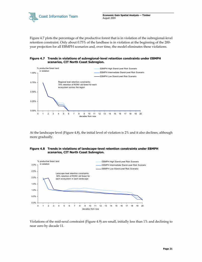
Figure 4.7 plots the percentage of the productive forest that is in violation of the subregional-level retention constraint. Only about 0.75% of the landbase is in violation at the beginning of the 200-year projection for all EBMPH scenarios and, over time, the model eliminates these violations.
Figure 4.7 Trends in violations of subregional-level retention constraints under EBMPH scenarios, CIT North Coast Subregion.
At the landscape level (Figure 4.8), the initial level of violation is 2% and it also declines, although more gradually.
Figure 4.8 Trends in violations of landscape-level retention constraints under EBMPH scenarios, CIT North Coast Subregion.
Violations of the mid-seral constraint (Figure 4.9) are small, initially less than 1% and declining to near zero by decade 11.
0.00%
0.25%
0.50%
0.75%
1.00%
0 1 2 3 4 5 6 7 8 9 10 11 12 13 14 15 16 17 18 19 20
EBMPH High Stand-Level Risk Scenario
EBMPH Intermediate Stand-Level Risk Scenario
EBMPH Low Stand-Level Risk Scenario
decades from now
% productive forest land in violation
Regional level retention constraints:70% retention of RONV old forest for each ecosystem across the region
0.0%
0.5%
1.0%
1.5%
2.0%
2.5%
3.0%
0 1 2 3 4 5 6 7 8 9 10 11 12 13 14 15 16 17 18 19 20
EBMPH High Stand-Level Risk Scenario
EBMPH Intermediate Stand-Level Risk Scenario
EBMPH Low Stand-Level Risk Scenario
decades from now
% productive forest land in violation
Lanscape level retention constraints: 50% retention of RONV old forest for each ecosystem in each landscape

Coast Information Team
Economic Gain Spatial Analysis — Timber August 2004
Page 22
Figure 4.9 Trends in violations of mid-seral retention constraints under EBMPH scenarios, CIT North Coast Subregion.
Note that the violations of the subregional and landscape retention constraints for the North Coast subregion are much smaller than on the Central Coast at the subregional level—0.75% versus 9.7%, and 2% versus 4.5%, respectively. Part of this difference is due to the amount of inoperable land in the productive forest landbase—84% of the productive forest of the North Coast subregion is inoperable, while 65% of the of the productive forest of the Central Coast is inoperable. The subregions also have different harvesting histories on the operable portions of their landbases.
The preponderance of inoperable land in the North Coast productive forest makes the comparison of age class distributions obtained under alternative scenarios (as in Figure 3.12) ineffective, and so is not included here.
0.00%
0.25%
0.50%
0.75%
1.00%
0 1 2 3 4 5 6 7 8 9 10 11 12 13 14 15 16 17 18 19 20
EBMPH High Stand-Level Risk Scenario
EBMPH Intermediate Stand-Level Risk Scenario
EBMPH Low Stand-Level Risk Scenario
decades from now
% productive forest land in violation
Mid seral constraints:Area of mid seral (age 40-120 years) must not exceed 50% of the productive forest, by ecosystem

Coast Information Team
Economic Gain Spatial Analysis — Timber August 2004
Page 23
4.3 Summary of Indicators — CIT North Coast Subregion
The indicators of timber value calculated for each landscape, and summed for the CIT North Coast LRMP Subregion are reported in Table 4.1. These indicators are described in section 3.5.
Table 4.1 Summary of indicators of timber value calculated with a price trend, CIT North Coast Subregion
TSR Base Case
Financial Efficiency
High Risk Intermediate
RiskLow Risk
Short Term (20 year)
Harvest Volume ('000 m3/year) 647 485 412 266 145
Employment - Jobs annual (LRMP) 211 158 134 87 47Employment - FTEs annual (LRMP) 550 412 349 226 123Employment - Jobs annual (BC) 345 259 220 142 77Employment - FTEs annual (BC) 20,460 46,883 21,610 13,769 6,101Employment Income (‘000 $/year) 3,508 2,625 2,222 1,437 782
Gross Revenue ('000 $/year) 84,260 87,583 57,510 37,369 20,401Delivered Wood Cost ('000 $/year) 63,800 40,700 35,900 23,600 14,300Net Revenue ('000 $/year) 20,460 46,883 21,610 13,769 6,101Rothery Stumpage ('000 $/year) 12,804 41,999 17,302 10,937 4,385Profit Allowance to Enterprise ('000 $/year) 7,656 4884 4308 2832 1716
Gross revenue ($/m3) 130.19 180.53 139.69 140.31 140.81Delivered Wood Cost ($/m3) 98.58 83.89 87.20 88.61 98.70Net Revenue ($/m3) 31.61 96.64 52.49 51.70 42.11Rothery Stumpage ($/m3) 19.78 86.57 42.03 41.06 30.26Profit Allowance to Enterprise ($/m3) 11.83 10.07 10.46 10.63 11.84
Long Term (200 years)
Harvest Volume ('000 m3/year) 554 485 412 266 145
Employment - Jobs annual (LRMP) 242 210 179 115 63Employment - FTEs annual (LRMP) 181 158 134 87 47Employment - Jobs annual (BC) 467 412 349 226 123Employment - FTEs annual (BC) 299 259 220 142 77Employment Income ‘000 ($/year) 8,614 7,490 6,360 4,114 2,238
Gross Revenue ('000 $/year) 109,224 101,291 86,186 55,753 30,535Delivered Wood Cost ('000 $/year) 54,500 43,800 37,300 24,300 14,100Net Revenue ('000 $/year) 54,724 57,491 48,886 31,453 16,435Rothery Stumpage ('000 $/year) 48,184 52,235 44,410 28,537 14,743Profit Allowance to Enterprise ('000 $/year) 6,540 5,256 4,476 2,916 1,692
Net Present Value ('000 000 $)
Gross Revenue ($/m3) 196.99 208.79 209.35 209.33 210.75Delivered Wood Cost ($/m3) 98.29 90.28 90.60 91.24 97.32Net Revenue ($/m3) 98.70 118.51 118.75 118.09 113.43Rothery Stumpage ($/m3) 86.90 107.67 107.87 107.15 101.76Profit Allowance to Enterprise ($/m3) 11.80 10.83 10.87 10.95 11.68
Ecosystem Based Management

Coast Information Team
Economic Gain Spatial Analysis — Timber August 2004
Page 24
The indicators summarized in Table 4.1, as well as the results reported elsewhere in section 4, were calculated using the price trend described in Appendix B. In order to facilitate the comparison of the North Coast subregion timber cost and revenue measures with the Central Coast (calculated without a price trend), the North Coast measures were recalculated without the price trend (Table 4.2).
The forecast short-term stumpage for the base case is $15.55 per m3, while the volume-weighted average stumpage collected in 2000-2002 was $4.16 per m3 for the North Coast TSA and $17.01 for TFL 25 (source: MoF).
Table 4.2 Summary of timber cost and revenue indicators calculated without a price trend, CIT North Coast Subregion
As with the Central Coast subregion, the revenue indicators for the North Coast are calculated with prices held constant at the top of the price cycle and, therefore, are best interpreted as indices rather than estimates of actual values.
TSR Base Case
Financial Efficiency
High Risk Intermediate
RiskLow Risk
Short Term (20 years)
Gross revenue ($/m3) 125.95 174.76 135.03 135.63 136.11Delivered Wood Cost ($/m3) 98.58 83.89 87.20 88.61 98.70Net Revenue ($/m3) 27.38 90.86 47.83 47.02 37.41Rothery Stumpage ($/m3) 15.55 80.80 37.36 36.39 25.57Profit Allowance to Enterprise ($/m3) 11.83 10.07 10.46 10.63 11.84
Long Term (20-200 years)
Gross revenue ($/m3) 129.98 136.81 136.43 136.44 137.85Delivered Wood Cost ($/m3) 98.29 90.28 90.60 91.24 97.32Net Revenue ($/m3) 31.69 46.52 45.83 45.20 40.54Rothery Stumpage ($/m3) 19.89 35.69 34.95 34.26 28.86Profit Allowance to Enterprise ($/m3) 11.80 10.83 10.87 10.95 11.68
Ecosystem Based Management

Coast Information Team
Economic Gain Spatial Analysis — Timber August 2004
Page 25
5.0 Results of Scenario Analysis — CIT Haida Gwaii Subregion
The CIT Haida Gwaii Subregion encompasses the Queen Charlotte TSA and TFL 25 Block 6, TFL 39 Block 6, and TFL 47 Block 18. The accompanying map (Figure 5.1) plots the boundaries of the region and the 42 CIT landscapes.
Figure 5.1 Map of the CIT Haida Gwaii Subregion and CIT landscapes.

Coast Information Team
Economic Gain Spatial Analysis — Timber August 2004
Page 26
5.1 Timber Harvest Values — CIT Haida Gwaii Subregion
The TSR base case harvest schedules for the individual management units that comprise the CIT Haida Gwaii matched closely to the harvest schedules determined for each unit by the EGSA-Timber model (not shown). The harvest schedule for the composite TSR base case for the subregion is plotted in Figure 5.2.
The impacts of the EBMPH scenarios with respect to the base case harvest levels are severe—the high stand-level risk scenario causes a 59% reduction in cut in the long term, the intermediate stand-level risk impact is 74%, and the low stand-level risk impact is 86%. These impacts exceed the reductions modelled on the North Coast and Central Coast and are due in part to the high proportion of second-growth timber on Haida Gwaii—EBMPH representation targets preserve older forest and force the cut to drop to levels that can be supported by the second growth.
Direct employment (FTEs) from harvesting, silviculture, and processing that is generated within the study area by the harvesting activity of the four scenarios is plotted on Figure 5.3. Although there are four management units in the CIT Haida Gwaii Subregion, they all share the same employment coefficients—hence the even flow of FTEs for scenarios producing an even flow of timber.
Figure 5.2 Harvest forecasts for all scenarios, CIT Haida Gwaii Subregion.
Figure 5.3 Direct employment forecast for all scenarios, within the CIT Haida Gwaii Subregion.
-200400600800
1,0001,2001,4001,6001,8002,0002,2002,400
0 1 2 3 4 5 6 7 8 9 10 11 12 13 14 15 16 17 18 19 20decades from now
TSR Base CaseFinancial Eff iciencyEBMPH High Stand-Level RiskEBMPH Intermediate Stand-Level RiskEBMPH Low Stand-Level Risk
volume ('000 m3 / year) Price assumptions:- top of cycle- price trend 0.3% annual
70% stand level 45% stand level
15% stand level
-
200
400
600
800
1,000
0 1 2 3 4 5 6 7 8 9 10 11 12 13 14 15 16 17 18 19 20decades from now
TSR Base CaseFinancial Eff iciencyEBMPH High Stand-Level Risk
EBMPH Intermediate Stand-Level RiskEBMPH Low Stand-Level Risk
FTEs / yearPrice assumptions:- top of cycle- price trend 0.3% annual
Coast Information Team
Economic Gain Spatial Analysis — Timber August 2004
Page 27
Other employment measures (direct FTEs outside the subregion, direct jobs inside and outside the subregion, and employment income) were also generated from the harvest time series, but add little information, so are not plotted here. These measures are included in the table of indicators at the end of this section.
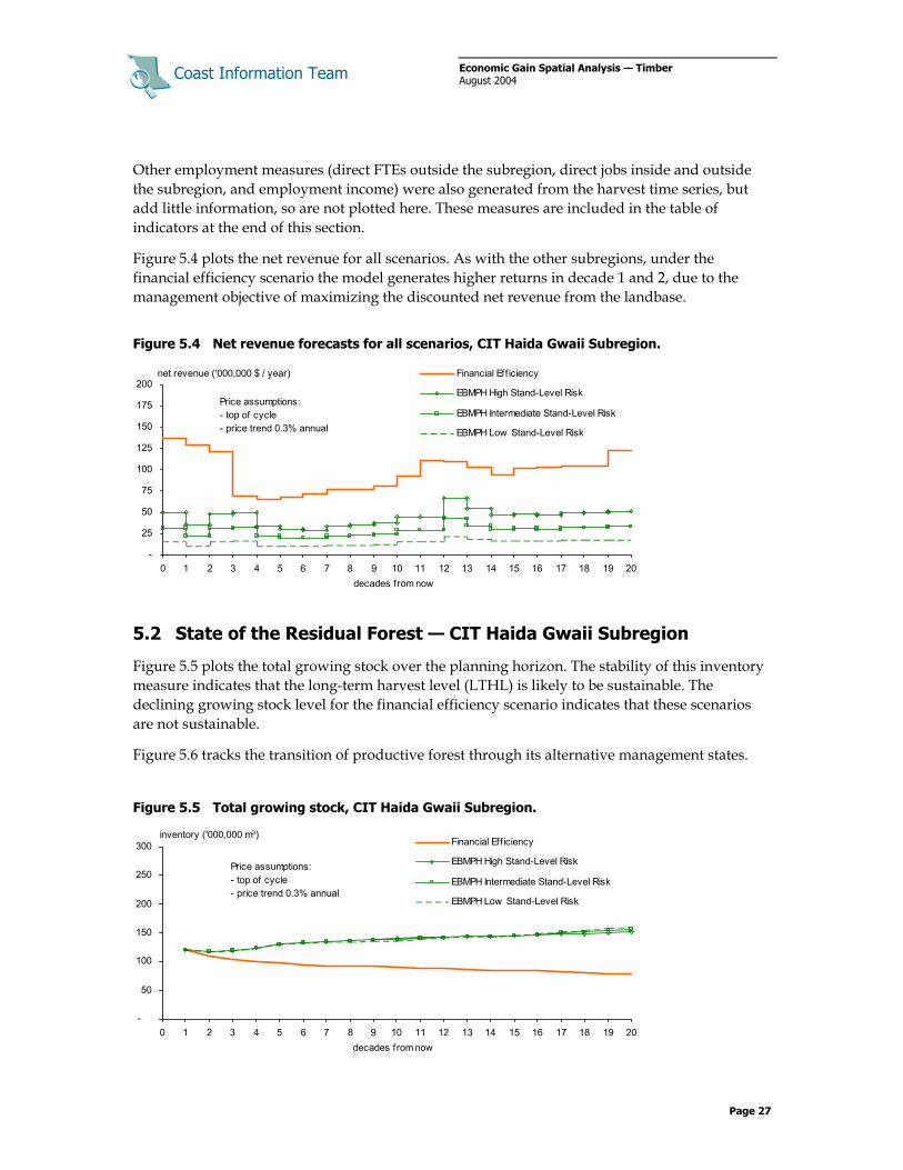
Figure 5.4 plots the net revenue for all scenarios. As with the other subregions, under the financial efficiency scenario the model generates higher returns in decade 1 and 2, due to the management objective of maximizing the discounted net revenue from the landbase.
Figure 5.4 Net revenue forecasts for all scenarios, CIT Haida Gwaii Subregion.
5.2 State of the Residual Forest — CIT Haida Gwaii Subregion
Figure 5.5 plots the total growing stock over the planning horizon. The stability of this inventory measure indicates that the long-term harvest level (LTHL) is likely to be sustainable. The declining growing stock level for the financial efficiency scenario indicates that these scenarios are not sustainable.
Figure 5.6 tracks the transition of productive forest through its alternative management states.
Figure 5.5 Total growing stock, CIT Haida Gwaii Subregion.
-
25
50
75
100
125
150
175
200
0 1 2 3 4 5 6 7 8 9 10 11 12 13 14 15 16 17 18 19 20decades from now
Financial Eff iciency
EBMPH High Stand-Level Risk
EBMPH Intermediate Stand-Level Risk
EBMPH Low Stand-Level Risk
net revenue ('000,000 $ / year)
Price assumptions:- top of cycle- price trend 0.3% annual
-
50
100
150
200
250
300
0 1 2 3 4 5 6 7 8 9 10 11 12 13 14 15 16 17 18 19 20decades from now
Financial Eff iciency
EBMPH High Stand-Level Risk
EBMPH Intermediate Stand-Level Risk
EBMPH Low Stand-Level Risk
inventory ('000,000 m3)
Price assumptions:- top of cycle- price trend 0.3% annual

Coast Information Team
Economic Gain Spatial Analysis — Timber August 2004
Page 28
Figure 5.6 Transition of the productive forest from natural and existing managed states to managed and retention states, CIT Haida Gwaii Subregion.
-
100
200
300
400
500
600
1 2 3 4 5 6 7 8 9 10 11 12 13 14 15 16 17 18 19 20
decades from now
Future managedExisting managedExisting naturalInoperable natural
area ('000 ha)
-
100
200
300
400
500
600
1 2 3 4 5 6 7 8 9 10 11 12 13 14 15 16 17 18 19 20
decades from now
Future managedExisting managedRetainedExisting naturalInoperable natural
area ('000 ha)
-
100
200
300
400
500
600
1 2 3 4 5 6 7 8 9 10 11 12 13 14 15 16 17 18 19 20
decades from now
Future managedExisting managedRetainedExisting naturalInoperable natural
area ('000 ha)
-
100
200
300
400
500
600
1 2 3 4 5 6 7 8 9 10 11 12 13 14 15 16 17 18 19 20
decades from now
Future managedExisting managedRetainedExisting naturalInoperable natural
area ('000 ha)
a. Financial Efficiency Scenario (FE) b. EBM High Stand-Level Risk Scenario
c. EBM Intermediate Stand-Level Risk d. EBM Low Stand-Level Risk Scenario

Coast Information Team
Economic Gain Spatial Analysis — Timber August 2004
Page 29
Figure 5.7 plots the percentage of the productive forest that is in violation of the subregional-level, landscape-level, and watershed-level retention constraints. The trends in percent violation do not vary perceptibly by EBMPH scenario and so are plotted on a single chart.
Figure 5.7 Trends in violations of the retention constraints under EBMPH scenarios, CIT Haida Gwaii Subregion.
About 10% of the productive forest land of the CIT Haida Gwaii Subregion is presently in violation of the subregional-level retention constraints, 5% violates the landscape-level constraints and 2% violates the watershed level constraints. The EBMPH scenarios all allow (up to) low environmental risk at the subregional level, intermediate risk at the landscape level and high risk at the watershed level. The model prevents additional violations of the retention constraints and eventually the desired distribution of old-seral ecosystems is attained.
The combination of retention constraints and the age class distribution of the THLB cause the severe reductions in harvest levels for the EBMPH constraints noted in section 5.1. The present level of violation of the retention constraints reflects the extensive harvesting that has occurred on Haida Gwaii—39 % of the THLB is less than 60 years of age and most of it will not be available for harvest in less than 60-80 years. The older forest withheld from harvest to prevent additional violations cannot be fully replaced by second growth, and the harvest level must be reduced.
To investigate the sensitivity of the harvest level to the degree of violation of the retention constraints we modified the penalty that the model applies to violations of the retention constraints. The penalty can be thought of as the relative importance of meeting retention constraints versus meeting harvest objectives, and in the EBMPH scenarios described above the penalty was assigned the value of 10,000:1, i.e., it was 10,000 times more important to prevent an additional hectare of violation than to harvest an additional cubic metre of timber.
In Figure 5.8 we plot the harvest level obtained by the model under the EMBPH High Stand-Level Risk scenario as we relax the importance from 10,000: 1 to 10:1, and the annual harvest level almost doubles from 723 thousand m3 to 1,347 thousand m3. The implications with respect to violations of the retention constraints is shown in Figure 5.9—the percent of productive forest land in violation of the retention constraints rises from current levels until decade 11, before dropping to zero.
0%
2%
4%
6%
8%
10%
12%
0 1 2 3 4 5 6 7 8 9 10 11 12 13 14 15 16 17 18 19 20 21 22 23 24 25decades from now
regional-level retentionconstraintslandscape-level retention constraintswatershed-level retention constraints
% of productive forest land in violation

Coast Information Team
Economic Gain Spatial Analysis — Timber August 2004
Page 30
Figure 5.8 Harvest levels obtained under the EBMPH High Stand-Level Risk scenario, with relaxed penalties for violating retention constraints, CIT Haida Gwaii Subregion.
Figure 5.9 Trends in violations of the retention constraints under EBMPH scenarios, with relaxed penalties, CIT Haida Gwaii Subregion.
0%
2%
4%
6%
8%
10%
12%
14%
16%
18%
0 1 2 3 4 5 6 7 8 9 10 11 12 13 14 15 16 17 18 19 20 21 22 23 24 25
decades from now
regional-level retention constraints
landscape-level retention constraints
watershed-level retention constraints
% of productive forest land in violation
-
200
400
600
800
1,000
1,200
1,400
1,600
10000:1 1000:1 100:1 20:1 10:1
harvest volume ('000 m3
/ )
importance of meeting EBMPH retention constraints vs. meeting harvest objectives
the harvest level obtained by the EBMPH High Stand-Level Risk scenario increases as the importance weight of meeting the old-seral constraints is reduced

Coast Information Team
Economic Gain Spatial Analysis — Timber August 2004
Page 31
5.3 Summary of Indicators — CIT Haida Gwaii Subregion
The indicators of timber value calculated for each landscape, and summed for the CIT Haida Gwaii Subregion are reported in Table 5.1. These indicators are described in section 3.5.
Table 5.1 Summary of indicators of timber value, CIT Haida Gwaii Subregion
TSR Base Case
Financial Efficiency
High Risk Intermediate
RiskLow Risk
Short Term (20 year)
Harvest Volume ('000 m3/year) 1,906 1,624 723 468 255
Employment - Jobs annual (LRMP) 953 812 361 234 128Employment - FTEs annual (LRMP) 572 487 217 140 77Employment - Jobs annual (BC) 1,906 1,624 723 468 255Employment - FTEs annual (BC) 1,811 1,543 687 444 242Employment Income (‘000 $/year) 27,757 23,653 10,523 6,809 3,714
Gross Revenue ('000 $/year) 254,865 278,201 107,735 69,530 37,937Delivered Wood Cost ('000 $/year) 170,300 140,700 63,800 41,800 24,200Net Revenue ('000 $/year) 84,565 137,501 43,935 27,730 13,737Rothery Stumpage ('000 $/year) 64,129 120,617 36,279 22,714 10,833Profit Allowance to Enterprise ('000 $/year) 20,436 16884 7656 5016 2904
Gross revenue ($/m3) 133.69 171.25 149.06 148.68 148.72Delivered Wood Cost ($/m3) 89.33 86.61 88.28 89.38 94.87Net Revenue ($/m3) 44.36 84.64 60.79 59.30 53.85Rothery Stumpage ($/m3) 33.64 74.25 50.20 48.57 42.47Profit Allowance to Enterprise ($/m3) 10.72 10.39 10.59 10.73 11.38
Long Term (200 years)
Harvest Volume ('000 m3/year) 1,757 1,624 723 468 255
Employment - Jobs annual (LRMP) 879 812 361 234 128Employment - FTEs annual (LRMP) 527 487 217 140 77Employment - Jobs annual (BC) 1,757 1,624 723 468 255Employment - FTEs annual (BC) 1,669 1,543 687 444 242Employment Income ‘000 ($/year) 25,587 23,653 10,523 6,809 3,714
Gross Revenue ('000 $/year) 316,407 294,270 133,738 86,567 47,263Delivered Wood Cost ('000 $/year) 153,200 138,000 62,300 40,400 22,600Net Revenue ('000 $/year) 163,207 156,270 71,438 46,167 24,663Rothery Stumpage ('000 $/year) 144,823 139,710 63,962 41,319 21,951Profit Allowance to Enterprise ('000 $/year) 18,384 16,560 7,476 4,848 2,712
Net Present Value ('000 000 $) 1,890 2,528 952 606 305
Gross Revenue ($/m3) 180.05 181.15 185.04 185.11 185.28Delivered Wood Cost ($/m3) 87.18 84.95 86.20 86.39 88.60Net Revenue ($/m3) 92.87 96.20 98.84 98.72 96.69Rothery Stumpage ($/m3) 82.41 86.00 88.50 88.35 86.05Profit Allowance to Enterprise ($/m3) 10.46 10.19 10.34 10.37 10.63
Ecosystem Based Management

Coast Information Team
Economic Gain Spatial Analysis — Timber August 2004
Page 32
As with the North Coast results (section 4), the indicators summarized in Table 5.1, as well as the results reported elsewhere in section 5, were calculated using the price trend described in Appendix B. In order to facilitate the comparison of the Haida Gwaii subregion timber cost and revenue measures with the North Coast (recalculated) and the Central Coast (calculated without a price trend), the Haida Gwaii measures were recalculated without the price trend (Table 5.2).
The forecast short-term stumpage for the base case is $29.09 per m3, while the volume-weighted average stumpage collected in 2000-2002 was $16.69 per m3 for the management units on the subregion (source: MoF).
Table 5.2 Summary of timber cost and revenue indicators calculated without a price trend, CIT Haida Gwaii Subregion
As with the other subregions reported in this study, the revenue indicators for Haida Gwaii are calculated with prices held constant at the top of the price cycle and, therefore, are best interpreted as indices rather than estimates of actual values.
TSR Base Case
Financial Efficiency
High Risk Intermediate
RiskLow Risk
Short Term (20 years)
Gross revenue ($/m3) 129.14 165.57 144.28 143.91 143.95Delivered Wood Cost ($/m3) 89.33 86.61 88.28 89.38 94.87Net Revenue ($/m3) 39.81 78.95 56.01 54.53 49.08Rothery Stumpage ($/m3) 29.09 68.56 45.42 43.80 37.70Profit Allowance to Enterprise ($/m3) 10.72 10.39 10.59 10.73 11.38
Long Term (20-200 years)
Gross revenue ($/m3) 116.15 118.13 120.29 120.25 120.43Delivered Wood Cost ($/m3) 87.18 84.95 86.20 86.39 88.60Net Revenue ($/m3) 28.97 33.18 34.09 33.86 31.83Rothery Stumpage ($/m3) 18.51 22.98 23.74 23.50 21.20Profit Allowance to Enterprise ($/m3) 10.46 10.19 10.34 10.37 10.63
Ecosystem Based Management

Coast Information Team
Economic Gain Spatial Analysis — Timber August 2004
Page 33
6.0 Comments on Sources of Uncertainty
The intent of this study is to inform planning tables about the value of forest lands under different management scenarios. The task of the planning tables is complicated by the deceptive nature of planning models, in particular, the EGSA-Timber model—in that they produce precise, long-term forecasts that are based on assumptions that increase in uncertainty with the passage of (modelled) time. Three sources of uncertainty in this analysis are discussed below, in descending order of importance.
6.1 Log Prices
We believe that the market conditions for coastal logs is the largest source of uncertainty in this study.
The prices obtained for logs from the CIT Central Coast Region reflects the prices offered for the products milled from those logs. These wood products, in turn, are subject to fluctuating demand and exchange rates, and must compete with other producers for market share.
Prices at the Vancouver Log Market vary widely in response to market conditions. For example over the last price cycle, the price of Douglas-fir ranged from $110 to $177/m3, and cedar from $60 to $140/m3. In addition to these cycles, the future price trend for coastal logs can only be extrapolated from past prices.
Market cycles, fluctuations in discount rates, and complex factors governing the development of future product demand (including trade barriers), when considered with the price sensitivity of the timber supply (Section 3.2.3), constitute the largest source of uncertainty with respect to the value of forest lands in this study. The results reported, including projections of stumpage and profit allowance to enterprise, do not take into account the price cycle since log prices are held constant at the top of the price cycle.
6.2 Harvesting Costs
The second largest source of uncertainty in this study is delivered wood costs. The trend in labour content of harvesting is clear (see Appendix C, Section C.2)—as industry substitutes capital (technology) for labour—but we can only speculate on the future shape of this trend. For example, at some point minimum labour requirements may be reached but technology costs—which to-date have been more than offset by decreasing labour costs—may continue to rise, increasing harvesting costs.
The long-term trend of internalizing costs to the environment through regulation will likely continue. An example included in this study is the effect on unit development costs of reducing the tributary volume harvested in each woodshed.
Changing harvest costs have the same (but inverse) effect as prices, and affect timber supply through the price-sensitivity mechanism discussed in the Sections 3.4.2 and 3.2.3. They are likely the second largest source of uncertainty with respect to the value of forest lands in this study.

Coast Information Team
Economic Gain Spatial Analysis — Timber August 2004
Page 34
The projections generated in this analysis do not take into account how the harvest might be affected by future land use decisions, such as a government-to-government agreement to set aside certain lands as tribal reserve or another form of protected area, or lands that might be withdrawn from the timber harvesting landbase for other purposes.
6.3 Forest Cover Data
Lack of confidence in the accuracy of the forest cover data, and site indices in particular, is a long-standing issue with resource planners and has been mentioned by both industry and environmental organizations during the development of this study. We agree that the forest cover data, which are fundamental to assessing the value attributable to harvesting, are a significant source of uncertainty with respect to the results of this project.

Coast Information Team
Economic Gain Spatial Analysis — Timber August 2004
Page 35
References
Anonymous. 2003. Woodshed Analysis for the North Coast LRMP (Draft). Report prepared for the North Coast LRMP by the Major Forest Licensee Sector. 15 p.
Coast Information Team. 2004. Ecosystem-Based Management Planning Handbook. 88 p.
Cortex Consultants Inc. 2004. Analysis of the impact on timber supply of the CFCI/RSP agreement. Report prepared for the Ministry of Forests, Coast Region, Nanaimo, B.C. 16 p.
Pearse, P.H. 2001. Ready for change: Crisis and opportunity in the coast forest industry. Report prepared for the Minister of Forests, British Columbia. 35 p.
Pierce Lefebvre Consulting and D.A. Ruffle & Associates Ltd. 2003. An analysis of woodflow in the Coast Forest Region. Report prepared for B.C. Ministry of Sustainable Resource Management, Victoria, B.C. 55 p.
Timberline Forest Inventory Consultants Ltd. 2000. Assessing current timber harvesting value in the Central Coast. Report prepared for B.C. Ministry of Forests, Vancouver Forest Region, Nanaimo, B.C. 26 p.
_____. 2002. Haida Gwaii / QCI Land Use Plan Woodshed Analysis. Report prepared for B.C. Ministry of Sustainable Resource Management, Coast Region, Nanaimo, B.C. 31 p.

Coast Information Team
Economic Gain Spatial Analysis — Timber August 2004
Page A-1
Appendix A. Implementation of the EGSA-Timber Forest-level Model
Table of Contents
A.1 Model Structure and Solution Method................................................................................... 4 A.2 Assembling the Landbase Model .......................................................................................... 4 A.3 Forming Analysis Units ........................................................................................................ 6 A.4 Generating Yield Curves .................................................................................................... 12 References ................................................................................................................................. 30
List of Yield Curves
A.1 Central Coast: AU 1 Fir, SI> 27, natural stands, TFLs ......................................................... 14
A.2 Central Coast: AU 2 Fir, 21≤ SI≤ 27, natural stands, TFLs.................................................... 14
A.3 Central Coast: AU 3 Fir, SI≤ 20, natural stands, TFLs. ......................................................... 14
A.4 Central Coast: AU 4 Cedar, SI> 23, natural stands, TFLs..................................................... 14
A.5 Central Coast: AU 5 Cedar, 16≤ SI≤ 23, natural stands, TFLs............................................... 14
A.6 Central Coast: AU 6 Cedar, SI≤ 15, natural stands, TFLs. .................................................... 14
A.7. Central Coast: AU 7 HemBal, SI> 22, natural stands, TFLs.................................................. 15
A.8 Central Coast: AU 8 HemBal, 12.6≤ SI≤ 22, natural stands, TFLs ......................................... 15
A.9 Central Coast: AU 9 HemBal, SI≤ 12.5, natural stands, TFLs................................................ 15
A.10 Central Coast: AU 10 Spruce, SI> 22, natural stands, TFLs ................................................. 15
A.11 Central Coast: AU 11 Spruce, 16≤ SI≤ 22, natural stands, TFLs ........................................... 15
A.12 Central Coast: AU 12 Spruce, SI≤ 16, natural stands, TFLs. ................................................. 15
A.13 Central Coast: AU 1 Fir, SI> 27, managed stands, TFLs ...................................................... 16
A.14 Central Coast: AU 2 Fir, 21≤ SI≤ 27, managed stands, TFLs ................................................ 16
A.15 Central Coast: AU 3 Fir, SI≤ 20, managed stands, TFLs....................................................... 16
A.16 Central Coast: AU 4 Cedar, SI> 23, managed stands, TFLs ................................................. 16
A.17 Central Coast: AU 5 Cedar, 16≤ SI≤ 23, managed stands, TFLs ........................................... 16
A.18 Central Coast: AU 6 Cedar, SI≤ 15, managed stands, TFLs. ................................................. 16
A.19 Central Coast: AU 7 HemBal, SI> 22, managed stands, TFLs............................................... 17
A.20 Central Coast: AU 8 HemBal, 12.6≤ SI≤ 22, managed stands, TFLs...................................... 17
A.21 Central Coast: AU 9 HemBal, SI≤ 12.5, managed stands, TFLs. ........................................... 17
A.22 Central Coast: AU 10 Spruce, SI> 22, managed stands, TFLs .............................................. 17
A.23 Central Coast: AU 11 Spruce, 16≤ SI≤ 22, managed stands, TFLs ........................................ 17
A.24 Central Coast: AU 12 Spruce, SI≤ 15, managed stands, TFLs............................................... 17
A.25. Central Coast: AU 1 Fir, SI> 27, natural stands, TSAs ......................................................... 18
A.26 Central Coast: AU 2 Fir, 21≤ SI≤ 27, natural stands, TSAs ................................................... 18

Coast Information Team
Economic Gain Spatial Analysis — Timber August 2004
Page A-2
A.27 Central Coast: AU 3 Fir, SI≤ 20, natural stands, TSAs.......................................................... 18
A.28 Central Coast: AU 4 Cedar, SI> 23, natural stands, TSAs .................................................... 18
A.29 Central Coast: AU 5 Cedar, 16≤ SI≤ 23, natural stands, TSAs .............................................. 18
A.30 Central Coast: AU 6 Cedar, SI≤ 15, natural stands, TSAs..................................................... 18
A.31 Central Coast: AU 7 HemBal, SI> 22, natural stands, TSAs ................................................. 19
A.32 Central Coast: AU 8 HemBal, 12.6≤ SI≤ 22, natural stands, TSAs......................................... 19
A.33 Central Coast: AU 9 HemBal, SI≤ 12.5, natural stands, TSAs. .............................................. 19
A.34 Central Coast: AU 10 Spruce, SI> 22, natural stands, TSAs................................................. 19
A.35 Central Coast: AU 11 Spruce, 16≤ SI≤ 22, natural stands, TSAs........................................... 19
A.36 Central Coast: AU 12 Sprucer, SI≤ 15, natural stands, TSAs. ............................................... 19
A.37 Central Coast: AU 1 Fir, SI> 27, managed stands, TSAs...................................................... 20
A.38 Central Coast: AU 2 Fir, 21≤ SI≤ 27, managed stands, TSAs................................................ 20
A.39 Central Coast: AU 3 Fir, SI≤ 20, managed stands, TSAs. ..................................................... 20
A.40 Central Coast: AU 4 Cedar, SI> 23, managed stands, TSAs................................................. 20
A.41 Central Coast: AU 5 Cedar, 16≤ SI≤ 23, managed stands, TSAs ........................................... 20
A.42 Central Coast: AU 6 Cedar, SI≤ 15, managed stands, TSAs. ................................................ 20
A.43 Central Coast: AU 7 HemBal, SI> 22, managed stands, TSAs .............................................. 21
A.44 Central Coast: AU 8 HemBal, 12.6≤ SI≤ 22, managed stands, TSAs ..................................... 21
A.45 Central Coast: AU 9 HemBal, SI≤ 12.5, managed stands, TSAs. ........................................... 21
A.46 Central Coast: AU 10 Spruce, SI> 22, managed stands, TSAs.............................................. 21
A.47 Central Coast: AU 11 Spruce, 16≤ SI≤ 22, managed stands, TSAs........................................ 21
A.48 Central Coast: AU 12 Spruce, SI≤ 15, managed stands, TSAs. ............................................. 21
A.49 North Coast: AU 1 Cedar, ITG+9,11,14, SI>22 .................................................................. 22
A.50 North Coast: AU 2 Cedar, ITG=9,11,14, 15≤ SI≤ 22............................................................ 22
A.51 North Coast: AU 3 Cedar, ITG=9,11,14, SI<15................................................................... 22
A.52 North Coast: AU 4 HemBalDecid, ITG= 12,15-20, 37, SI>22 .............................................. 22
A.53 North Coast: AU 5 HemBalDecid, (thinned) ITG= 12,15-20,37, SI>22 ................................. 22
A.54 North Coast: AU 6 HemBaldecid, ITG= 12, 15-20, 37, 15≤ SI≤ 22 ....................................... 22
A.55 North Coast: AU 7 HemBalDecid (thinned), ITG= 12, 15-20, 37, 15≤ SI≤ 22 ........................ 23
A.56 North Coast: AU 8 HemBalDecid, ITG=12, 15-20, 37, SI<15 ............................................... 23
A.57 North Coast: AU 9 Spruce, ITG=21,23,24,26, SI>22........................................................... 23
A.58 North Coast: AU 10 Spruce, ITG= 21, 23, 24, 26, 15≤ SI≤ 22.............................................. 23
A.59 North Coast: AU 11 Spruce, ITG 21,23,24,26, SI<15 .......................................................... 23
A.60 North Coast: AU 12 Cottonwood, ITG= 35,36, SI= all ......................................................... 23
A.61 HG/QCI: AU 1 Cedar, ITG 9-11, SI≥ 15 .............................................................................. 24
A.62 HG/QCI: AU 2 Cedar, ITG 9-11, SI= 12.5-14.99 ................................................................. 24
A.63 HG/QCI: AU 3 Cedar, ITG 9-11, SI< 12.5........................................................................... 24
A.64 HG/QCI: AU 4 Hemlock, ITG 12-20, SI≥ 18 ........................................................................ 24
A.65 HG/QCI: AU 5 Hemlock, ITG 12-20, SI= 15-17.99 .............................................................. 24
A.66 HG/QCI: AU 6 Hemlock, ITG 12-20, SI< 15........................................................................ 24
A.67 HG/QCI: AU 7 Spruce, ITG 21-26, SI≥ 16........................................................................... 25

Coast Information Team
Economic Gain Spatial Analysis — Timber August 2004
Page A-3
A.68 HG/QCI: AU 8 Spruce, ITG 21-26, SI< 16 .......................................................................... 25
A.69 HG/QCI: TFL 25: AU1 Cedar, ITG 9-11, SI≥ 15 ................................................................... 25
A.70 HG/QCI: TFL 25: AU 2 Cedar, ITG 9-11, SI= 12.5-14.99 ..................................................... 25
A.71 HG/QCI: TFL 25: AU 3 Cedar, ITG 9-11, S< 12.5................................................................ 25
A.72 HG/QCI: TFL 25: AU 4 Hemlock, ITG 12-20, SI≥ 18 ........................................................... 26
A.73 HG/QCI: TFL 25: AU 5 Hemlock, ITG 12-20, SI= 15-17.99 .................................................. 26
A.74 HG/QCI: TFL 25: AU 6 Hemlock, ITG 12-20, SI<15 ............................................................ 26
A.75 HG/QCI: TFL 25: AU 7 Spruce, ITG 21-26, SI≥ 16............................................................... 26
A.76 HG/QCI: TFL 25: AU 8 Spruce, ITG 21-26, SI< 16 .............................................................. 26
A.77 HG/QCI: TFL 39: AU 1 Cedar, ITG 9-11, SI≥ 15 ................................................................. 27
A.78 HG/QCI: TFL 39: AU 2 Cedar, ITG 9-11, SI= 12.5-14.99 ..................................................... 27
A.79 HG/QCI: TFL 39: AU 3 Cedar, ITG 9-11, SI< 12.5 .............................................................. 27
A.80 HG/QCI: TFL 39: AU 4 Hemlock, ITG 12-20, SI≥ 18 ............................................................ 27
A.81 HG/QCI: TFL 39: AU 5 Hemlock, ITG 12-20, SI= 15-17.99 .................................................. 27
A.82 HG/QCI: TFL 39: AU 6 Hemlock, ITG 12-20, SI< 15 ........................................................... 27
A.83 HG/QCI: TFL 39: AU 7 Spruce, ITG 21-26, SI≥ 16 .............................................................. 28
A.84 HG/QCI: TFL 39: AU 8 Spruce, ITG 21-26, SI< 16 .............................................................. 28
A.85 HG/QCI: TFL 47: AU 1 Cedar, ITG 9-11, SI≥ 15.................................................................. 28
A.86 HG/QCI: TFL 47: AU 2 Cedar, ITG 9-11, SI= 12.5-14.99 ..................................................... 28
A.87 HG/QCI: TFL 47: AU 3 Cedar, ITG 9-11, SI< 12.5 .............................................................. 28
A.88 HG/QCI: TFL 47: AU 4 Hemlock, ITG 12-20, SI≥ 18 ............................................................ 29
A.89 HG/QCI: TFL 47: AU 5 Hemlock, ITG 12-20, SI 15-17.99 .................................................... 29
A.90 HG/QCI: TFL 47: AU 6 Hemlock, ITG 12-20, SI< 15 ........................................................... 29
A.91 HG/QCI: TFL 47: AU 7 Spruce, ITG 21-26, SI≥ 16............................................................... 29
A.92 HG/QCI: TFL 47: AU 8 Spruce, ITG 21-26, SI< 16.............................................................. 29
List of Tables
A.1 Coverages used to create the model landbase ...................................................................... 5
A.2 Classification of the forest landbase ..................................................................................... 5
A.3 Definition of the analysis units, by CIT region....................................................................... 6
A.4 Classification the productive forest landbase by analysis unit, operability, and site index......... 8
A.5 Productive forest land by CIT region, BEC variant and analysis unit. .................................... 10
A.6 Utilization levels for yield models. ...................................................................................... 12
A.7 TIPSY input assumptions by CIT region.............................................................................. 12

Coast Information Team
Economic Gain Spatial Analysis — Timber August 2004
Page A-4
A.1 Model Structure and Solution Method
A major difference between this forest-level analysis and most analyses undertaken for the TSR is the choice of the forest estate model. For Crown-managed lands (TSAs), the TSR uses FSSIM, a forest-level simulator, and most major licensees (TFLs) use proprietary simulation models. This analysis casts the harvest scheduling problem as a linear model, solvable by linear programming (LP). Woodstock was used to create the LP model and an optimization code (MOSEK) was used to solve it.1
An LP model represents the forest and its management as a series of linear equations, which can be arranged in a matrix. One equation, the objective function, expresses the forest-level objective (e.g., maximize volume production or maximize net present value). Other equations represent the forest management rules such as limits on harvest fluctuation and forest cover constraints. The LP solution software finds the set of management activities (e.g., harvesting) that best meet the objective. The reader is referred to Davis et al. (2001) for an overview of LP formulations for forest-level planning.
Separate models were developed for each of the three CIT regions: Central Coast, North Coast and Haida Gwaii/Queen Charlotte Islands (QCI).
We selected an LP modelling approach for this study because linear models require that the management objective is explicitly stated and that the results generated by the model optimize this objective. Other authors (e.g., Messmer 1994a, 1994b) have used the Woodstock modelling system for economic studies of the forest resource in British Columbia.
Implementing the forest-level model involves four major activities:
1. Specifying the objectives, constraints, activities, state transitions, and outputs of the model
2. Assembling and integrating the various landbase coverages
3. Forming analysis units
4. Generating yield curves
The first activity, building the model within the Woodstock framework, is dealt with in other parts of this report. The objectives and constraints are specified by scenario and documented in Appendix D, and the state transitions and outputs are described in the Results section (Section 3.0) of the main report. The other three activities are described in the following sections of this appendix.
A.2 Assembling the Landbase Model
Three coverages were combined to create the model landbase. Coverages used in the model are listed in Table A.1.
1 MOSEK is a product of MOSEK ApS, Copenhagen, Denmark. Woodstock/Stanley is a product of RemSoft Ltd., Fredericton, N.B. http://www.remsoft.com/

Coast Information Team
Economic Gain Spatial Analysis — Timber August 2004
Page A-5
Table A.1 Coverages used to create the model landbase.
Description of coveragea Source 1. Forest cover – includes growth and yield data, BEC zone, NDT,
landscape units, operability, watersheds, VQOs, protected areas MSRM Nanaimo
2. Woodsheds MSRM Nanaimo 3. Landscapes CIT 4. Watershedsb Nature Conservancy, Victoria a See Table A.2 for definitions. b Watersheds were not included in the CIT Central Coast Region model landbase.
The landbase is classified in the according to 16 themes (Table A.2) for decision-making and indexing inputs and outputs.
Table A.2 Classification of the forest landbase.
Landbase themes Description Purpose
Analysis units aggregates of inventory types and site classes (Table 2)
groups forest area into yield classes that can be adequately represented with a single yield table
Management unit/Woodshed/Landscape unit
self-explanatory identifies TSA or TFL/a contiguous area for which access, development costs, and grade distributions have been determined/provincial landscape unit
Block self-explanatory identifies the inventory block within a TFL
Landscape self-explanatory identifies the CIT landscape
Watershed provincial 3rd-order watersheds identifies the 3rd order watersheds
Operability self-explanatory determines whether forest area is within the THLB (operable) or is inoperable
BEC biogeoclimatic ecological classification zone
assign forest cover constraints to the landbase
NDT natural disturbance type assign forest cover constraints to the landbase
VQO visual quality objective - defines a level of acceptable landscape alteration
assign forest cover constraints to the landbase
DWR deer winter range - presence or absence of deer management area
assign forest cover constraints to the landbase
Grizzly presence or absence of grizzly bear habitat
assign forest cover constraints to the landbase
Community watershed presence or absence of community watershed
assign forest cover constraints to the landbase
Inner/outer coast location constraint ensures minimum volume of timber is harvested from the outer coast
Harvesting method conventional/helicopter constraints ensure harvest method ratio
Management state natural/managed indicates yield model to be used for volume yield forecasts
Age age in decades (Figure 4) forecast forest development over time

Coast Information Team
Economic Gain Spatial Analysis — Timber August 2004
Page A-6
A.3 Forming Analysis Units
Analysis units (Table A.3), which are aggregates of forest area with similar growth and yield characteristics, were defined for each of the study regions.
Table A.3 Definition of the analysis units, by CIT region
Analysis unit Inventory type and site breaks
Inoperable (ha)
Operable (ha)
CIT Central Coast Region
AU1 Fir, ITG=1–8, SI >27 5,516 30,558
AU2 Fir, ITG=1–8, 21<= SI <=27 14,911 31,880
AU3 Fir, ITG=1–8, SI <=20 21,874 11,082
AU4 Cedar SI >23 4,294 13,906
AU5 Cedar, ITG=9–11, 16<= SI <=23 78,157 97,278
AU6 Cedar, ITG=9–11, SI <=15 549,799 75,322
AU7 HemBal, ITG=12–20, SI >22 53,809 158,551
AU8 HemBal, ITG=12–20, 12.6<= SI <=22 248,999 216,973
AU9 HemBal, ITG=12–20, SI <=12.5 244,453 15,238
AU10 Spruce, ITG=21–26, SI >22 3,529 7,480
AU11 Spruce, ITG=21–26, 16<= SI <=22 4,046 8,616
AU12 Spruce, ITG=21–26, SI <=15, Pine ITG 21-34 24,899 3,069
AU13 Decid, ITG=35–42, SI = all 33,240 14,021
Total area CIT Central Coast Region 1,287,526 683,973
CIT North Coast Region
AU1 Cedar, ITG=9,11,14, SI >22 322 1164
AU2 Cedar, ITG=9,11,14, 15<= SI <=22 9939 12141
AU3 Cedar, ITG=9,11,14, SI <15 402567 36746
AU4 HemBalDecid, ITG= 12,15,16,17,18,19,20,37, SI >22 6448 10611
AU5 HemBalDecid, (thinned) ITG= 12,15,16,17,18,19,20,37, SI >22 20 130
AU6 HemBalDecid, ITG= 12,15,16,17,18,19,20,37, 15<= SI <=22 21118 27846
AU7 HemBalDecid (thinned), ITG= 12,15,16,17,18,19,20,37, 15<= SI <=22 211 1220
AU8 HemBalDecid, ITG= 12,15,16,17,18,19,20,37, SI <15 150989 29756
AU9 Spruce, ITG= 21,23,24,26, SI >22 1498 2274
AU10 Spruce, ITG= 21,23,24,26, 15<= SI <=22 2204 4638
AU11 Spruce, ITG= 21,23,24,26, SI <15 5749 2688
AU12 Cottonwood, ITG= 35,36, SI = all 445 268
AU13 Cedar fir, ITG=10, SI = all 62900
AU14 Pine, ITG = 27-34, SI = all 17127
Total area CIT North Coast Region 681,538 129,842

Coast Information Team
Economic Gain Spatial Analysis — Timber August 2004
Page A-7
Table A.3 (continued)
Analysis unit Inventory type and site breaks
Inoperable (ha)
Operable (ha)
CIT Haida Gwaii Region
AU1 Cedar, ITG 9-11, SI >=15 27,697 36,695
AU2 Cedar, ITG 9-11, SI 12.5-14.99 17,849 17,566
AU3 Cedar, ITG 9-11, SI <12.5 165,823 17,048
AU4 Hemlock, ITG 12-20, SI >=18 38,319 85,326
AU5 Hemlock, ITG 12-20, SI 15-17. 21,667 18,660
AU6 Hemlock, ITG 12-20, SI <15 61,593 23,409
AU7 Spruce, ITG 21-26, SI >=16 17,405 33,710
AU8 Spruce, ITG 21-26, SI <16 13,111 7,346
AU9 Pine, ITG 28-31, All 7,431 -
AU10 Deciduous, ITG 37,38, All 7,346 -
Total area CIT Haida Gwaii Region 378,240 239,760
1ITG –inventory type group
SI –site index
Table A.4 reports the productive forest landbase by analysis unit, operability class, and site index, and Table A.5 report the same landbase by BEC label (as recorded in the MSRM planning resultants coverage) and analysis unit.

Coast Information Team
Economic Gain Spatial Analysis — Timber August 2004
Page A-8
Table A.4 Productive forest land by CIT region, analysis unit, operability, and site index.
CIT Central Coast RegionManagement Inoperable Operable Weighted Management Inoperable Operable Weighted Unit Analysis Unit (ha) THLB (ha) Total (ha) Site Index Unit Analysis Unit (ha) THLB (ha) Total (ha) Site IndexMid Coast SAU1 - Fir, ITG 1-8, SI >27 748 1,677 2,425 30.8 TFL 251 SAU1 - Fir, ITG 1-8, SI >27 49 739 788 35.3 Mid Coast SAU2 - Fir, ITG 1-8, SI 21-27 5,993 7,061 13,054 23.2 TFL 25 SAU2 - Fir, ITG 1-8, SI 21-27 1 18 19 24.4 Mid Coast SAU3 - Fir, ITG 1-8, SI <=20 11,201 2,015 13,216 19.7 TFL 25 SAU3 - Fir, ITG 1-8, SI <=20 - - - - Mid Coast SAU4 - Cedar, ITG 9-11, SI >23 442 1,358 1,800 26.0 TFL 25 SAU4 - Cedar, ITG 9-11, SI >23 698 630 1,328 24.3 Mid Coast SAU5 - Cedar, ITG 9-11, SI 16-23 30,407 31,876 62,284 18.4 TFL 25 SAU5 - Cedar, ITG 9-11, SI 16-23 10,439 18,353 28,793 19.1 Mid Coast SAU6 - Cedar, ITG 9-11, SI <=15 251,350 16,346 267,696 14.0 TFL 25 SAU6 - Cedar, ITG 9-11, SI <=15 32,966 11,338 44,303 12.0 Mid Coast SAU7 - HemBal, ITG 12-20, SI >22 4,935 11,962 16,897 25.4 TFL 25 SAU7 - HemBal, ITG 12-20, SI >22 24,715 35,184 59,900 28.6 Mid Coast SAU8 - HemBal, ITG 12-20, SI 12.6-22 134,518 109,624 244,141 18.8 TFL 25 SAU8 - HemBal, ITG 12-20, SI 12.6-22 9,992 1,772 11,764 17.7 Mid Coast SAU9 - HemBal, ITG 12-20, SI <=12.5 141,357 5,621 146,978 11.8 TFL 25 SAU9 - HemBal, ITG 12-20, SI <=12.5 4,714 189 4,904 12.0 Mid Coast SAU10 - Spruce, ITG 21-26, SI >22 1,290 4,334 5,623 30.1 TFL 25 SAU10 - Spruce, ITG 21-26, SI >22 699 1,354 2,053 34.4 Mid Coast SAU11 - Spruce, ITG 21-26, SI 16-22 2,120 4,292 6,412 17.5 TFL 25 SAU11 - Spruce, ITG 21-26, SI 16-22 2 15 17 22.0 Mid Coast SAU12 - Spruce, SI <= 15, Pine ITG 21-34, All SI 10,230 1,934 12,164 12.8 TFL 25 SAU12 - Spruce, SI <= 15, Pine ITG 21-34, All SI 56 - 56 - Mid Coast SAU13 - Decid, ITG 35-42, SI all 11,955 3,293 15,248 24.8 TFL 25 SAU13 - Decid, ITG 35-42, SI all 489 1,022 1,510 26.1
Total Mid Coast 606,546 201,393 807,939 Total TFL 25 84,819 70,615 155,434 Kingcome SAU1 - Fir, ITG 1-8, SI >27 675 501 1,176 30.7 TFL 392 SAU1 - Fir, ITG 1-8, SI >27 14 45 59 39.0 Kingcome SAU2 - Fir, ITG 1-8, SI 21-27 3,858 1,074 4,932 25.6 TFL 39 SAU2 - Fir, ITG 1-8, SI 21-27 322 546 867 21.0 Kingcome SAU3 - Fir, ITG 1-8, SI <=20 6,419 86 6,505 13.6 TFL 39 SAU3 - Fir, ITG 1-8, SI <=20 14 34 48 20.0 Kingcome SAU4 - Cedar, ITG 9-11, SI >23 2,181 7,304 9,485 28.1 TFL 39 SAU4 - Cedar, ITG 9-11, SI >23 701 1,807 2,508 27.0 Kingcome SAU5 - Cedar, ITG 9-11, SI 16-23 26,782 33,525 60,307 19.9 TFL 39 SAU5 - Cedar, ITG 9-11, SI 16-23 4,174 3,930 8,105 20.3 Kingcome SAU6 - Cedar, ITG 9-11, SI <=15 185,773 33,830 219,603 14.0 TFL 39 SAU6 - Cedar, ITG 9-11, SI <=15 5,757 5,420 11,177 15.0 Kingcome SAU7 - HemBal, ITG 12-20, SI >22 16,190 42,781 58,970 28.2 TFL 39 SAU7 - HemBal, ITG 12-20, SI >22 2,868 9,978 12,847 29.1 Kingcome SAU8 - HemBal, ITG 12-20, SI 12.6-22 70,379 46,044 116,423 19.5 TFL 39 SAU8 - HemBal, ITG 12-20, SI 12.6-22 10,434 7,619 18,053 20.0 Kingcome SAU9 - HemBal, ITG 12-20, SI <=12.5 57,213 2,171 59,384 11.4 TFL 39 SAU9 - HemBal, ITG 12-20, SI <=12.5 284 309 594 10.8 Kingcome SAU10 - Spruce, ITG 21-26, SI >22 738 1,104 1,842 29.5 TFL 39 SAU10 - Spruce, ITG 21-26, SI >22 494 280 774 29.0 Kingcome SAU11 - Spruce, ITG 21-26, SI 16-22 1,481 3,828 5,309 20.4 TFL 39 SAU11 - Spruce, ITG 21-26, SI 16-22 189 96 284 18.6 Kingcome SAU12 - Spruce, SI <= 15, Pine ITG 21-34, All SI 11,757 228 11,985 12.9 TFL 39 SAU12 - Spruce, SI <= 15, Pine ITG 21-34, All SI 78 45 123 22.0 Kingcome SAU13 - Decid, ITG 35-42, SI all 15,885 1,176 17,061 27.0 TFL 39 SAU13 - Decid, ITG 35-42, SI all 166 181 346 32.7
Total Kingcome 399,329 173,653 572,982 Total TFL 39 25,496 30,288 55,784 Strathcona SAU1 - Fir, ITG 1-8, SI >27 3,652 20,513 24,164 32.3 TFL 453 SAU1 - Fir, ITG 1-8, SI >27 189 776 965 29.3 Strathcona SAU2 - Fir, ITG 1-8, SI 21-27 3,597 14,208 17,805 24.9 TFL 45 SAU2 - Fir, ITG 1-8, SI 21-27 821 2,383 3,204 22.7 Strathcona SAU3 - Fir, ITG 1-8, SI <=20 2,681 5,434 8,115 17.2 TFL 45 SAU3 - Fir, ITG 1-8, SI <=20 1,134 992 2,126 18.0 Strathcona SAU4 - Cedar, ITG 9-11, SI >23 160 913 1,073 27.5 TFL 45 SAU4 - Cedar, ITG 9-11, SI >23 69 334 403 27.8 Strathcona SAU5 - Cedar, ITG 9-11, SI 16-23 2,573 4,097 6,670 19.1 TFL 45 SAU5 - Cedar, ITG 9-11, SI 16-23 1,512 2,163 3,675 18.6 Strathcona SAU6 - Cedar, ITG 9-11, SI <=15 8,751 2,223 10,974 11.9 TFL 45 SAU6 - Cedar, ITG 9-11, SI <=15 739 421 1,159 13.6 Strathcona SAU7 - HemBal, ITG 12-20, SI >22 2,911 16,169 19,080 28.1 TFL 45 SAU7 - HemBal, ITG 12-20, SI >22 1,548 4,873 6,421 26.7 Strathcona SAU8 - HemBal, ITG 12-20, SI 12.6-22 8,622 26,028 34,650 18.9 TFL 45 SAU8 - HemBal, ITG 12-20, SI 12.6-22 9,864 10,819 20,683 18.8 Strathcona SAU9 - HemBal, ITG 12-20, SI <=12.5 8,722 1,232 9,954 10.8 TFL 45 SAU9 - HemBal, ITG 12-20, SI <=12.5 17,577 3,420 20,997 10.4 Strathcona SAU10 - Spruce, ITG 21-26, SI >22 20 43 63 27.7 TFL 45 SAU10 - Spruce, ITG 21-26, SI >22 187 105 292 28.1 Strathcona SAU11 - Spruce, ITG 21-26, SI 16-22 - - - - TFL 45 SAU11 - Spruce, ITG 21-26, SI 16-22 156 152 308 20.0 Strathcona SAU12 - Spruce, SI <= 15, Pine ITG 21-34, All SI 1,336 - 1,336 - TFL 45 SAU12 - Spruce, SI <= 15, Pine ITG 21-34, All SI 246 257 503 13.9 Strathcona SAU13 - Decid, ITG 35-42, SI all 1,375 4,692 6,067 26.7 TFL 45 SAU13 - Decid, ITG 35-42, SI all 2,828 27 2,855 -
Total Strathcona 44,399 95,554 139,952 Total TFL 45 36,869 26,720 63,589 North Coast SAU1 - Fir, ITG 1-8, SI >27 - - - - TFL 474 SAU1 - Fir, ITG 1-8, SI >27 190 6,308 6,498 34.5 North Coast SAU2 - Fir, ITG 1-8, SI 21-27 - - - - TFL 47 SAU2 - Fir, ITG 1-8, SI 21-27 320 6,590 6,910 27.0 North Coast SAU3 - Fir, ITG 1-8, SI <=20 - - - - TFL 47 SAU3 - Fir, ITG 1-8, SI <=20 425 2,521 2,946 18.6 North Coast SAU4 - Cedar, ITG 9-11, SI >23 40 65 106 37.6 TFL 47 SAU4 - Cedar, ITG 9-11, SI >23 3 1,495 1,498 26.6 North Coast SAU5 - Cedar, ITG 9-11, SI 16-23 2,213 2,144 4,357 21.9 TFL 47 SAU5 - Cedar, ITG 9-11, SI 16-23 57 1,188 1,245 16.0 North Coast SAU6 - Cedar, ITG 9-11, SI <=15 64,374 2,933 67,307 13.3 TFL 47 SAU6 - Cedar, ITG 9-11, SI <=15 90 2,812 2,902 10.0 North Coast SAU7 - HemBal, ITG 12-20, SI >22 175 547 723 24.3 TFL 47 SAU7 - HemBal, ITG 12-20, SI >22 465 37,056 37,522 28.5 North Coast SAU8 - HemBal, ITG 12-20, SI 12.6-22 4,591 5,595 10,186 18.1 TFL 47 SAU8 - HemBal, ITG 12-20, SI 12.6-22 599 9,472 10,071 17.0 North Coast SAU9 - HemBal, ITG 12-20, SI <=12.5 14,475 1,131 15,606 11.5 TFL 47 SAU9 - HemBal, ITG 12-20, SI <=12.5 111 1,163 1,274 11.0 North Coast SAU10 - Spruce, ITG 21-26, SI >22 102 121 223 25.2 TFL 47 SAU10 - Spruce, ITG 21-26, SI >22 - 138 138 32.0 North Coast SAU11 - Spruce, ITG 21-26, SI 16-22 98 231 329 20.0 TFL 47 SAU11 - Spruce, ITG 21-26, SI 16-22 - 2 2 19.0 North Coast SAU12 - Spruce, SI <= 15, Pine ITG 21-34, All SI 1,057 84 1,142 12.8 TFL 47 SAU12 - Spruce, SI <= 15, Pine ITG 21-34, All SI 139 520 659 14.6 North Coast SAU13 - Decid, ITG 35-42, SI all 516 - 516 - TFL 47 SAU13 - Decid, ITG 35-42, SI all 27 3,631 3,658 32.2
Total North Coast 87,643 12,853 100,496 Total TFL 47 2,426 72,897 75,323
Total TSA Area 1,137,916 483,453 1,621,369 Total TFL Area 149,610 200,520 350,130
Total TFL Area 149,610 200,520 350,130 1 TFL 25 - Blocks 2 and 52 TFL 39 - Blocks 3, 5, and 7
Total CIT Central Coast Area 1,287,526 683,973 1,971,500 3 TFL 45 - All Blocks4 TFL 47 - Johnstone Strait

Coast Information Team
Economic Gain Spatial Analysis — Timber August 2004
Page A-9
Table A.4 continued
CIT North Coast Region CIT Haida Gwaii Region
Management UnitAnalysis Unit
Inoperable (ha)
Operable THLB (ha) Total (ha) Weighted
Site Index Management UnitAnalysis Unit
Inoperable (ha)
Operable THLB (ha)
North Coast TSA AU1 - Cedar, ITG=9,11,14, SI >22 322 1,164 1,486 25.1 QCI TSA AU1:Cedar, ITG 9-11, SI >=15 6,450 10,485 North Coast TSA AU2 - Cedar, ITG=9,11,14, 15<= SI <=22 9,781 11,951 21,733 18.8 QCI TSA AU2:Cedar, ITG 9-11, SI 12.5-14.99 12,570 11,043 North Coast TSA AU3 - Cedar, ITG=9,11,14, SI <15 399,170 36,495 435,665 12.9 QCI TSA AU3:Cedar, ITG 9-11, SI <12.5 152,896 9,231 North Coast TSA AU4 - HemBalDecid, ITG= 12,15,16,17,18,19,20,37, SI >22 4,180 5,771 9,951 26.5 QCI TSA AU4: Hemlock, ITG 12-20, SI >=18 7,904 11,021 North Coast TSA AU5 - HemBalDecid, (thinned) ITG= 12,15,16,17,18,19,20,37, SI >22 20 130 149 26.2 QCI TSA AU5: Hemlock, ITG 12-20, SI 15-17.99 11,264 8,043 North Coast TSA AU6 - HemBalDecid, ITG= 12,15,16,17,18,19,20,37, 15<= SI <=22 18,348 27,461 45,808 19.0 QCI TSA AU6: Hemlock, ITG 12-20, SI <15 53,969 18,517 North Coast TSA AU7 - HemBalDecid (thinned), ITG= 12,15,16,17,18,19,20,37, 15<= SI <=22 211 1,220 1,432 22.0 QCI TSA AU7: Spruce, ITG 21-26, SI >=16 6,666 6,783 North Coast TSA AU8 - HemBalDecid, ITG= 12,15,16,17,18,19,20,37, SI <15 146,938 29,756 176,694 13.5 QCI TSA AU8: Spruce, ITG 21-26, SI <16 11,936 6,798 North Coast TSA AU9 - Spruce, ITG= 21,23,24,26, SI >22 1,419 2,021 3,440 26.9 QCI TSA AU9: Pine, ITG 28-31, All 6,443 North Coast TSA AU10 - Spruce, ITG= 21,23,24,26, 15<= SI <=22 2,198 4,632 6,829 19.7 QCI TSA AU10: Deciduous, ITG 37,38, All 1,895 North Coast TSA AU11 - Spruce, ITG= 21,23,24,26, SI <15 5,745 2,688 8,433 12.6 Total QCI TSA 271,993 81,923 North Coast TSA AU12 - Cottonwood, ITG= 35,36, SI = all 445 268 713 41.1North Coast TSA AU13 - Cedar fir, ITG=10, SI = all 62,900 - 62,900 n/a TFL 25, Block 6 AU1:Cedar, ITG 9-11, SI >=15 1,859 1,924 North Coast TSA AU14 - Pine, ITG = 27-34, SI = all 17,127 - 17,127 n/a TFL 25, Block 6 AU2:Cedar, ITG 9-11, SI 12.5-14.99 1,935 785
Total North Coast TSA 668,805 123,556 792,361 TFL 25, Block 6 AU3:Cedar, ITG 9-11, SI <12.5 8,310 729 TFL 25, Block 6 AU4: Hemlock, ITG 12-20, SI >=18 1,662 9,884
TFL 25, Block 5 AU1 - Cedar, ITG=9,11,14, SI >22 - - - n/a TFL 25, Block 6 AU5: Hemlock, ITG 12-20, SI 15-17.99 1,654 1,551 TFL 25, Block 5 AU2 - Cedar, ITG=9,11,14, 15<= SI <=22 157 190 348 18.8 TFL 25, Block 6 AU6: Hemlock, ITG 12-20, SI <15 3,897 1,470 TFL 25, Block 5 AU3 - Cedar, ITG=9,11,14, SI <15 3,397 251 3,648 12.9 TFL 25, Block 6 AU7: Spruce, ITG 21-26, SI >=16 889 7,073 TFL 25, Block 5 AU4 - HemBalDecid, ITG= 12,15,16,17,18,19,20,37, SI >22 2,269 4,840 7,109 26.5 TFL 25, Block 6 AU8: Spruce, ITG 21-26, SI <16 566 202 TFL 25, Block 5 AU5 - HemBalDecid, (thinned) ITG= 12,15,16,17,18,19,20,37, SI >22 - - - n/a TFL 25, Block 6 AU9: Pine, ITG 28-31, All 38 - TFL 25, Block 5 AU6 - HemBalDecid, ITG= 12,15,16,17,18,19,20,37, 15<= SI <=22 2,770 385 3,155 19.0 TFL 25, Block 6 AU10: Deciduous, ITG 37,38, All 2,079 - TFL 25, Block 5 AU7 - HemBalDecid (thinned), ITG= 12,15,16,17,18,19,20,37, 15<= SI <=22 - - - n/a Total TFL 25 22,889 23,617 TFL 25, Block 5 AU8 - HemBalDecid, ITG= 12,15,16,17,18,19,20,37, SI <15 4,051 - 4,051 13.5TFL 25, Block 5 AU9 - Spruce, ITG= 21,23,24,26, SI >22 79 253 333 26.9 TFL 39, Block 6 AU1:Cedar, ITG 9-11, SI >=15 17,379 21,365 TFL 25, Block 5 AU10 - Spruce, ITG= 21,23,24,26, 15<= SI <=22 7 6 13 19.7 TFL 39, Block 6 AU2:Cedar, ITG 9-11, SI 12.5-14.99 3,319 5,737 TFL 25, Block 5 AU11 - Spruce, ITG= 21,23,24,26, SI <15 3 - 3 12.6 TFL 39, Block 6 AU3:Cedar, ITG 9-11, SI <12.5 3,044 6,801 TFL 25, Block 5 AU12 - Cottonwood, ITG= 35,36, SI = all - - - n/a TFL 39, Block 6 AU4: Hemlock, ITG 12-20, SI >=18 26,339 56,025 TFL 25, Block 5 AU13 - Cedar fir, ITG=10, SI = all - - - n/a TFL 39, Block 6 AU5: Hemlock, ITG 12-20, SI 15-17.99 8,714 9,027 TFL 25, Block 5 AU14 - Pine, ITG = 27-34, SI = all - - - n/a TFL 39, Block 6 AU6: Hemlock, ITG 12-20, SI <15 3,437 3,070
Total TFL 25 12,733 5,925 18,658 TFL 39, Block 6 AU7: Spruce, ITG 21-26, SI >=16 8,877 14,636 TFL 39, Block 6 AU8: Spruce, ITG 21-26, SI <16 585 233
Total CIT North Coast Area 681,538 129,482 811,020 TFL 39, Block 6 AU9: Pine, ITG 28-31, All 950 - TFL 39, Block 6 AU10: Deciduous, ITG 37,38, All 2,965 -
Total TFL 39 75,609 116,894
TFL 47, Block 18 AU1:Cedar, ITG 9-11, SI >=15 2,009 2,921 TFL 47, Block 18 AU2:Cedar, ITG 9-11, SI 12.5-14.99 24 1 TFL 47, Block 18 AU3:Cedar, ITG 9-11, SI <12.5 1,573 286 TFL 47, Block 18 AU4: Hemlock, ITG 12-20, SI >=18 2,414 8,396 TFL 47, Block 18 AU5: Hemlock, ITG 12-20, SI 15-17.99 34 38 TFL 47, Block 18 AU6: Hemlock, ITG 12-20, SI <15 291 353 TFL 47, Block 18 AU7: Spruce, ITG 21-26, SI >=16 972 5,217 TFL 47, Block 18 AU8: Spruce, ITG 21-26, SI <16 23 114 TFL 47, Block 18 AU9: Pine, ITG 28-31, All - - TFL 47, Block 18 AU10: Deciduous, ITG 37,38, All 407 -
Total TFL 39 7,748 17,326
Total CIT QCI Area 378,240 239,760

Coast Information Team
Economic Gain Spatial Analysis — Timber August 2004
Page A-10
Table A.5 Productive forest land by CIT region, BEC variant and analysis unit
CIT Central Coast Region
BEC AU 1 AU 2 AU 3 AU 4 AU 5 AU 6 AU 7 AU 8 AU 9 AU 10 AU 11 AU 12 AU 13 Grand TotalFir Fir Fir Cedar Cedar Cedar HemBal HemBal HemBal Spruce Pine Spruce Pine Spruce Pine Deciduous
ITG 1-8 ITG 1-8 ITG=1-8 ITG=9-11 ITG=9-11 ITG=9-11 ITG=12-20 ITG=12-20 ITG=12-20 ITG=21-34 ITG=21-34 ITG=21-34 ITG=35-42
SI>2721<= SI <=27 SI <=20 SI >23
16<= SI <=23 SI <=15 SI >22
12.6<= SI <=22 SI <=12.5 SI >22
16<= SI <=22 SI <15 SI = all
AT 30 136 39 158 900 8 1,270 CWHdm 2,050 1,756 614 262 658 671 6,718 2,283 196 76 930 16,214 CWHds2 754 5,928 6,908 197 1,793 281 775 9,881 3,578 67 54 5,869 2,700 38,784 CWHmm1 624 1,670 1,402 45 724 878 4,629 10,957 1,806 148 96 22,980 CWHmm2 15 155 124 182 322 669 3,859 1,625 6,951 CWHms2 2,040 8,377 7,111 800 6,165 3,896 7,392 59,196 12,182 1,435 867 1,905 7,567 118,933 CWHvh1 11 163 4,418 15,751 124,363 9,975 20,815 8,266 577 2,452 2,350 2,218 191,359 CWHvh2 27 990 44,737 242,202 20,861 38,370 21,927 1,936 1,095 2,813 3,355 378,313 CWHvm 32 1,223 5,852 1,508 4,727 3,025 99 55 30 179 16,732 CWHvm1 5,400 8,189 3,001 10,443 82,386 136,727 125,637 142,905 28,746 6,371 6,235 4,010 22,747 582,795 CWHvm2 158 337 212 522 15,612 81,713 11,335 57,120 42,617 25 740 566 662 211,617 CWHvm3 53 274 416 20 1,419 2,078 413 20,142 13,699 4 132 122 48 38,821 CWHws2 76 2,389 3,812 50 1,438 607 2,236 53,087 32,363 351 756 3,513 926 101,604 CWHxm 3 80 33 7 35 258 183 9 608 CWHxm1 6,776 2,167 920 35 21 278 256 10 5 172 1,112 11,752 CWHxm2 18,042 13,928 5,921 318 519 731 18,048 7,316 736 60 872 3,006 69,496 ESSFmc 393 140 1,263 1,796 ESSFmk 78 55 133 ESSFmw 1 123 1,742 2,142 978 4,985 ESSFmwh 24 41 21 86 IDFww 1,219 1,780 280 35 25 738 294 79 2,557 606 7,611 MHmm1 2 96 38 1,362 15,457 815 13,394 36,320 2 65 42 46 67,640 MHmm2 71 299 52 277 92 15,241 39,925 19 49 494 6 56,525 MHmm2e 2 106 250 3 361 MHmmp 10 17 27 MHwh 188 1,852 87 698 2,451 1 8 3 5,289 MHwh1 79 2,653 184 484 4 3,404 not classified 73 59 183 24 782 4,390 569 2,109 5,895 57 81 148 1,042 15,413 Grand Total 36,074 46,790 32,956 18,200 175,435 625,122 212,360 465,973 259,691 11,010 12,661 27,967 47,261 1,971,500

Coast Information Team
Economic Gain Spatial Analysis — Timber August 2004
Page A-11
Table A.5 continued
CIT North Coast RegionBEC AU1 AU2 AU3 AU4 AU5 AU6 AU7 AU8 AU9 AU10 AU11 AU12 AU13 AU14 Grand Total
Cedar Cedar Cedar Hemlock Hemlock 2 Hemlock Hemlock b Hemlock Spruce Spruce Spruce Cottonwood Cedar, fir PineITG 9,11,14 ITG 9,11,14 ITG 9,11,14 ITGa ITGa ITGa ITGa ITGa ITG 21,23,24,26 ITG 21,23,24,26 ITG 21,23,24,26 ITG 35,36 ITG 10 ITG 27-33
SI > 22 SI 15-22 SI < 15 SI > 22 SI > 22 SI 15-22 SI 15-22 SI < 15 SI > 22 SI 15-22 SI < 15 All All All TotalAT 18 2 571 591 CWHvh2 747 12,465 290,090 2,099 5 12,628 1,162 32,726 545 1,864 3,411 61,860 16,978 436,581 CWHvm 473 3,792 58,906 4,932 5 17,886 186 54,760 2,072 3,714 3,376 91 149 3 150,346 CWHvm1 182 2,548 10,767 6,852 127 4,210 18 3,306 505 323 40 196 11 29,087 CWHvm2 353 5,361 814 12 2,052 4,046 8 9 18 12 12,684 CWHwm 43 1,954 34,003 881 6,455 28,413 593 781 981 347 54 74,505 CWHws1 4 4 204 678 2,021 2,405 16 42 24 262 5,661 CWHws2 123 1,360 321 1,599 7,414 12 28 17 4 10,878 MHmm1 27 239 14,064 338 1,090 27,414 17 34 217 9 1 43,450 MHmm2 34 598 48 301 9,191 4 10,176 MHwh 10 568 23,941 96 720 65 10,500 4 42 353 628 133 37,060 Grand Total 1,486 22,080 439,313 17,060 149 48,963 1,432 180,745 3,773 6,842 8,436 713 62,900 17,127 811,020
a ITG - 12,15,16,17,18,19,20,37b Thinned stands
CIT Haida Gwaii Region.BEC AU1 AU2 AU3 AU4 AU5 AU6 AU7 AU8 AU9 AU10 Grand Total
1:Cedar 2:Cedar 3:Cedar 4: Hemlock 5: Hemlock 6: Hemlock 7: Spruce 8: Spruce 9: Pine 10: DeciduousITG 9-11 ITG 9-11 ITG 9-11 ITG 12-20 ITG 12-20 ITG 12-20 ITG 21-26 ITG 21-26 ITG 28-31 ITG 37,38SI >=15 I 12.5-14.99 SI <12.5 SI >=18 SI 15-17.99 SI <15 SI >=16 SI <16 All All Total
AT 27 91 14 23 164 23 343 CWHvh2 6,409 7,494 58,053 11,579 13,474 43,240 8,859 9,621 544 1,281 160,553 CWHwh1 48,260 25,025 108,584 90,357 14,424 23,081 37,770 7,084 6,811 5,848 367,244 CWHwh2 7,943 2,340 10,901 18,991 9,092 10,660 3,388 2,082 63 114 65,575 MHwh 1,410 192 1,283 1,856 1,775 1,737 327 201 1 8,783 MHwh1 129 165 2,535 230 895 4,189 147 577 14 8,880 MHwh2 156 114 1,145 279 408 1,303 114 380 3,901 ZZZZ 57 83 278 337 236 628 509 488 102 2,720 Grand Total 64,393 35,415 182,870 123,645 40,327 85,002 51,115 20,457 7,431 7,346 617,999

Coast Information Team
Economic Gain Spatial Analysis — Timber August 2004
Page A-12
A.4 Generating Yield Curves
Forest management assumptions—including forest cover requirements, utilization levels and standards, unsalvaged losses, and green-up assumptions—are generally unchanged from the TSR and management plan timber supply analyses.
VDYP (Variable Density Yield Projection System; B.C. Ministry of Forests 1996) was used to forecast yields for stands of natural origin and TIPSY (Table Interpolation Program for Sustained Yield; Di Lucca 1999) was used to forecast yields from managed stands. Tables A.6 and A.7 list the inputs and assumptions used in the yield project.
Table A.6 Utilization levels for yield modelsa
VDYP TIPSY Minimum dbh 17.5 12.5 Maximum stump 30 30 Minimum top dib 10 10 a All figures are in centimetres.
Table A.7 TIPSY input assumptions by CIT region
CIT Central Coast Region
Analysis
Regeneration
Planting stock
Operational adjustment factorsb
unit Species Site index Percent Type Lag Age (years) Density OAF1 OAF2
1 Fdc M WSIa 100 Planted 2 1 1200 0.85 0.95 2 Fdc M WSI 100 Planted 2 1 1200 0.85 0.95 3 Fdc M WSI 100 Planted 2 1 1200 0.85 0.95 4 Cw M WSI 100 Planted 2 1 1200 0.85 0.95 5 Cw M WSI 100 Planted 2 1 1200 0.85 0.95 6 Cw M WSI 100 Planted 2 1 1200 0.85 0.95 7 Hwc M WSI 100 Planted 2 1 1200 0.85 0.95 8 Hwc M WSI 100 Planted 2 1 1200 0.85 0.95 9 Hwc M WSI 100 Planted 2 1 1200 0.85 0.95
10 Ss M WSI 100 Planted 2 1 1200 0.85 0.95 11 Ss M WSI 100 Planted 2 1 1200 0.85 0.95 12 Ss M WSI 100 Planted 2 1 1200 0.85 0.95
CIT North Coast Region
Analysis
Regeneration
Planting Stock
Thinned
Operational adjustment factors
Unit Species Site Index Type Lag Age (years) Density Density OAF1 OAF2 1 Cw/Hwc WSIc Natural 1 1 10000+ 0.85 0.95 2 Cw/Hwc WSI Natural 1 1 10000+ 0.85 0.95 3 Cw/Hwc WSI Natural 1 1 10000+ 0.85 0.95 4 Hwc WSI Natural 2 1 10000+ 0.85 0.95 5 Hwc WSI Natural 2 1 10000+ 700 0.85 0.95 6 Hwc WSI Natural 2 1 10000+ 0.85 0.95 7 Hwc WSI Natural 2 1 10000+ 700 0.85 0.95 8 Hwc WSI Natural 2 1 10000+ 0.85 0.95 9 Ss WSI Planted 2 1 1000 0.85 0.95
10 Ss WSI Planted 2 1 10000+ 0.85 0.95 11 Ss WSI Natural 2 1 10000+ 0.85 0.95 12 Acd WSI Planted 1 1 1200 0.85 0.95

Coast Information Team
Economic Gain Spatial Analysis — Timber August 2004
Page A-13
CIT Haida Gwaii Region
Analysis New AU
Regeneration
Planting Stock
Thinned Operational
Adjustment Factors Unit Species # % Type Lag Age (years) Density Density OAF1 OAF2
1 Cw 1 25 Plant 5 1 15000 1600 0.85 0.95 Ss 7 75 Plant 5 1 15000 1600 0.85 0.95
2 Cw 2 50 Plant 5 1 3000 1600 0.85 0.95 Hwc 6 50 Plant 5 1 7000 1600 0.85 095
3 Cw 3 100 Plant 5 1 2000 n/a 0.85 0.95 4 Hwc 4 100 Natural 3 1 20000 1600 0.85 0.95 5 Hwc 5 100 Natural 3 1 20000 1600 0.85 0.95 6 Hwc 6 100 Natural 5 1 30000 1600 0.85 0.95 7 Ss 7 70 Natural 3 1 15000 1600 0.85 0.95 Hwc 5 30 Natural 3 1 15000 1600 0.85 0.95
8 Ss 3 100 Plant 3 1 3000 700 0.85 0.95 a Weighted site index by management type (Crown vs. TFL), calculated from immature (age 41–140) natural stands for TFLs and TSAs in the CIT Central Coast Region.
b OAF –operational adjustment factors used to adjust yield curves for stocking differences and endemic losses. c Weighted site index calculated for the for the immature stands of the North Coast LRMP area. d Interior Douglas-fir used as substitute.
For the CIT Central Coast Region, sets of VDYP and TIPSY yield curves were developed for the Crown-managed lands (Timber Supply Areas) and TFLs. The site indices for each management type were calculated as the area-weighted average site index of the immature natural stands.
The VDYP and TIPSY input parameters and yield curves for the CIT North Coast Region were adopted without change from the North Coast LRMP Timber Supply Analysis (North Coast Government Technical Team, 2002).
The Haida Gwaii /QCI yield tables were adopted without change from the Queen Charlotte Islands TSA Timber Supply Analysis (B.C. Ministry of Forests, 2000). Yields for the TFLs were calculated from the TSA curves by applying scale factors, where the scale factors were determined by comparing published TSA and TFL curves.
Figures A.1 to A.92 plot the yield curves used in this study

Coast Information Team
Economic Gain Spatial Analysis — Timber August 2004
Page A-14
0
200
400
600
800
1000
1200
1400
10 20 30 40 50 60 70 80 90 100 110 120 130 140 150 160 170 180 190 200
age (years)
TFL 25
TFL 39
TFL 45
TFL 47
0
100
200
300
400
500
600
700
800
900
1000
10 20 30 40 50 60 70 80 90 100 110 120 130 140 150 160 170 180 190 200
age (years)
TFL 25
TFL 39
TFL 45
TFL 47
0
100
200
300
400
500
600
10 20 30 40 50 60 70 80 90 100 110 120 130 140 150 160 170 180 190 200
age (years)
TFL 39
TFL 45
TFL 47
m3/ha
0
200
400
600
800
1000
1200
10 20 30 40 50 60 70 80 90 100 110 120 130 140 150 160 170 180 190 200
age (years)
TFL 25
TFL 39
TFL 45
TFL 47
0
100
200
300
400
500
600
700
800
10 20 30 40 50 60 70 80 90 100 110 120 130 140 150 160 170 180 190 200
age (years)
TFL 25
TFL 39
TFL 45
TFL 47
0
50
100
150
200
250
300
350
400
450
500
10 20 30 40 50 60 70 80 90 100 110 120 130 140 150 160 170 180 190 200
age (years)
TFL 25
TFL 39
TFL 45
TFL 47
m3/ha
Figure A.1 Central Coast: AU 1 Fir, SI >27, natural stands, TFLs.
Figure A.3 Central Coast: AU 3 Fir, SI <= 20, natural stands, TFLs.
Figure A.2 Central Coast: AU 2 Fir, 21<= SI <=27, natural stands, TFLs.
Figure A.4 Central Coast: AU 4 Cedar SI >23, natural stands, TFLs.
Figure A.6 Central Coast: AU 6 Cedar, SI <=15, natural stands, TFLs.
Figure A.5 Central Coast: AU 5 Cedar, 16<= SI <=23, natural stands, TFLs.

Coast Information Team
Economic Gain Spatial Analysis — Timber August 2004
Page A-15
Figure A.7 Central Coast: AU 7 HemBal, SI >22, natural stands, TFLs.
Figure A.9 Central Coast: AU 9 HemBal, SI <= 12.5, natural stands, TFLs.
Figure A.8 Central Coast: AU 8 HemBal, 12.6<= SI <=22, natural stands, TFLs.
Figure A.10 Central Coast: AU 10 Spruce SI >22, natural stands, TFLs.
Figure A.12 Central Coast: AU 12 Spruce, SI <=16, natural stands, TFLs.
Figure A.11 Central Coast: AU 11 Spruce, 16<= SI <=22, natural stands, TFLs.
0 200 400 600 800
1000 1200
10 20 30 40 50 60 70 80 90 100 110 120 130 140 150 160 170 180 190 200age (years)
TFL 25 TFL 39 TFL 45 TFL 47
0 100 200 300 400 500 600 700 800
10 20 30 40 50 60 70 80 90 100 110 120 130 140 150 160 170 180 190 200age (years)
TFL 25 TFL 39 TFL 45 TFL 47
0 50
100 150 200 250 300 350 400 450 500
10 20 30 40 50 60 70 80 90 100 110 120 130 140 150 160 170 180 190 200
age (years)
TFL 25 TFL 39 TFL 45 TFL 47
m 3 /ha
0
200
400
600
800
1000
1200
1400
1600
10 20 30 40 50 60 70 80 90 100 110 120 130 140 150 160 170 180 190 200age (years)
TFL 25
TFL 39
TFL 45
TFL 47
0
100
200
300
400
500
600
700
800
900
1000
10 20 30 40 50 60 70 80 90 100 110 120 130 140 150 160 170 180 190 200age (years)
TFL 25
TFL 39
TFL 45
0
100
200
300
400
500
600
700
800
10 20 30 40 50 60 70 80 90 100 110 120 130 140 150 160 170 180 190 200
age (years)
TFL 39
TFL 45
TFL 47
m3/ha

Coast Information Team
Economic Gain Spatial Analysis — Timber August 2004
Page A-16
0
200
400
600
800
1000
1200
1400
1600
10 20 30 40 50 60 70 80 90 100 110 120 130 140 150 160 170 180 190 200
age (years)
TFL 25
TFL 39
TFL 45
TFL 47
0
100
200
300
400
500
600
700
800
900
1000
10 20 30 40 50 60 70 80 90 100 110 120 130 140 150 160 170 180 190 200
age (years)
TFL 25
TFL 39
TFL 45
TFL 47
0
100
200
300
400
500
600
700
10 20 30 40 50 60 70 80 90 100 110 120 130 140 150 160 170 180 190 200
age (years)
TFL 25
TFL 39
TFL 45
TFL 47
m3/ha
0
200
400
600
800
1000
1200
1400
1600
1800
2000
10 20 30 40 50 60 70 80 90 100 110 120 130 140 150 160 170 180 190 200
age (years)
TFL 25
TFL 39
TFL 45
TFL 47
0
200
400
600
800
1000
1200
10 20 30 40 50 60 70 80 90 100 110 120 130 140 150 160 170 180 190 200
age (years)
TFL 25
TFL 39
TFL 45
TFL 47
0
100
200
300
400
500
600
10 20 30 40 50 60 70 80 90 100 110 120 130 140 150 160 170 180 190 200
age (years)
TFL 25
TFL 39
TFL 45
TFL 47
m3/ha
Figure A.13 Central Coast: AU 1 Fir, SI >27, managed stands, TFLs.
Figure A.15 Central Coast: AU 3 Fir, SI <= 20, managed stands, TFLs.
Figure A.14 Central Coast: AU 2 Fir, 21<= SI <=27, managed stands, TFLs.
Figure A.16 Central Coast: AU 4 Cedar SI >23, managed stands, TFLs.
Figure A.18 Central Coast: AU 6 Cedar, SI <=15, managed stands, TFLs.
Figure A.17 Central Coast: AU 5 Cedar, 16<= SI <=23, managed stands, TFLs.

Coast Information Team
Economic Gain Spatial Analysis — Timber August 2004
Page A-17
0
200
400
600
800
1000
1200
1400
1600
1800
2000
10 20 30 40 50 60 70 80 90 100 110 120 130 140 150 160 170 180 190 200
age (years)
TFL 25
TFL 39
TFL 45
TFL 47
0
200
400
600
800
1000
1200
10 20 30 40 50 60 70 80 90 100 110 120 130 140 150 160 170 180 190 200
age (years)
TFL 25
TFL 39
TFL 45
TFL 47
0
50
100
150
200
250
300
350
400
450
500
10 20 30 40 50 60 70 80 90 100 110 120 130 140 150 160 170 180 190 200
age (years)
TFL 25
TFL 39
TFL 45
TFL 47
m3/ha
0
200
400
600
800
1000
1200
1400
1600
1800
10 20 30 40 50 60 70 80 90 100 110 120 130 140 150 160 170 180 190 200
age (years)
TFL 25
TFL 39
TFL 45
TFL 47
0
200
400
600
800
1000
1200
1400
1600
10 20 30 40 50 60 70 80 90 100 110 120 130 140 150 160 170 180 190 200
age (years)
TFL 25
TFL 39
TFL 45
TFL 47
0
200
400
600
800
1000
1200
1400
10 20 30 40 50 60 70 80 90 100 110 120 130 140 150 160 170 180 190 200
age (years)
TFL 25
TFL 39
TFL 45
TFL 47
m3/ha
Figure A.19 Central Coast: AU 7 HemBal, SI >22, managed stands, TFLs.
Figure A.21 Central Coast: AU 9 HemBal, SI <= 12.5, managed stands, TFLs.
Figure A.20 Yield curves: AU 8 HemBal, 12.6<= SI <=22, managed stands, TFLs.
Figure A.22 Central Coast: AU 10 Spruce, SI >22, managed stands, TFLs.
Figure A.24 Central Coast: AU 12 Spruce, SI <=15, managed stands, TFLs.
Figure A.23 Central Coast: AU 11 Spruce, 16<= SI <=22, managed stands, TFLs.

Coast Information Team
Economic Gain Spatial Analysis — Timber August 2004
Page A-18
0
200
400
600
800
1000
1200
10 20 30 40 50 60 70 80 90 100 110 120 130 140 150 160 170 180 190 200
age (years)
Mid CoastKingcomeStrathconaNorth Coast
0
100
200
300
400
500
600
700
10 20 30 40 50 60 70 80 90 100 110 120 130 140 150 160 170 180 190 200
age (years)
Mid CoastKingcomeStrathconaNorth Coast
0
50
100
150
200
250
300
350
400
450
10 20 30 40 50 60 70 80 90 100 110 120 130 140 150 160 170 180 190 200
age (years)
Mid CoastKingcomeStrathconaNorth Coast
m3/ha
0
200
400
600
800
1000
1200
10 20 30 40 50 60 70 80 90 100 110 120 130 140 150 160 170 180 190 200
age (years)
Mid Coast
Kingcome
Strathcona
0
100
200
300
400
500
600
700
800
10 20 30 40 50 60 70 80 90 100 110 120 130 140 150 160 170 180 190 200
age (years)
Mid Coast
Kingcome
Strathcona
0
50
100
150
200
250
300
350
400
450
500
10 20 30 40 50 60 70 80 90 100 110 120 130 140 150 160 170 180 190 200
age (years)
Mid Coast
Kingcome
Strathcona
m3/ha
Figure A.25 Central Coast: AU 1 Fir, SI >27, natural stands, TSAs.
Figure A.27 Central Coast: AU 3 Fir, SI <= 20, natural stands, TSAs.
Figure A.26 Central Coast: AU 2 Fir, 21<= SI <=27, natural stands, TSAs.
Figure A.28 Central Coast: AU 4 Cedar SI >23, natural stands, TSAs.
Figure A.30 Central Coast: AU 6 Cedar, SI <=15, natural stands, TSAs.
Figure A.29 Central Coast: AU 5 Cedar, 16<= SI <=23, natural stands, TSAs.

Coast Information Team
Economic Gain Spatial Analysis — Timber August 2004
Page A-19
0
200
400
600
800
1000
1200
10 20 30 40 50 60 70 80 90 100 110 120 130 140 150 160 170 180 190 200
age (years)
Mid CoastKingcomeStrathconaNorth Coast
0
100
200
300
400
500
600
700
10 20 30 40 50 60 70 80 90 100 110 120 130 140 150 160 170 180 190 200
age (years)
Mid CoastKingcomeStrathconaNorth Coast
0
50
100
150
200
250
300
350
400
450
10 20 30 40 50 60 70 80 90 100 110 120 130 140 150 160 170 180 190 200
age (years)
Mid CoastKingcomeStrathconaNorth Coast
m3/ha
0
200
400
600
800
1000
1200
10 20 30 40 50 60 70 80 90 100 110 120 130 140 150 160 170 180 190 200
age (years)
Mid CoastKingcomeStrathconaNorth Coast
0
100
200
300
400
500
600
700
800
900
1000
10 20 30 40 50 60 70 80 90 100 110 120 130 140 150 160 170 180 190 200
age (years)
Mid Coast
Kingcome
North Coast
0
100
200
300
400
500
600
700
10 20 30 40 50 60 70 80 90 100 110 120 130 140 150 160 170 180 190 200
age (years)
Mid Coast
Kingcome
North Coast
m3/ha
Figure A.31 Central Coast: AU 7 HemBal, SI >22, natural stands, TSAs.
Figure A.33 Central Coast: AU 9 HemBal, SI <= 12.5, natural stands, TSAs.
Figure A.32 Central Coast: AU 8 HemBal, 12.6<= SI <=22, natural stands, TSAs.
Figure A.34 Central Coast: AU 10 Spruce, SI >22, natural stands, TSAs.
Figure A.36 Central Coast: AU 12 Spruce, SI <=15, natural stands, TSAs.
Figure A.35 Central Coast: AU 11 Spruce, 16<= SI <=22, natural stands, TSAs.

Coast Information Team
Economic Gain Spatial Analysis — Timber August 2004
Page A-20
0
200
400
600
800
1000
1200
1400
10 20 30 40 50 60 70 80 90 100 110 120 130 140 150 160 170 180 190 200
age (years)
Mid Coast
Kingcome
Strathcona
0
100
200
300
400
500
600
700
800
900
1000
10 20 30 40 50 60 70 80 90 100 110 120 130 140 150 160 170 180 190 200
age (years)
Mid Coast
Kingcome
Strathcona
0
100
200
300
400
500
600
10 20 30 40 50 60 70 80 90 100 110 120 130 140 150 160 170 180 190 200
age (years)
Mid Coast
Kingcome
Strathcona
m3/ha
0
500
1000
1500
2000
2500
3000
10 20 30 40 50 60 70 80 90 100 110 120 130 140 150 160 170 180 190 200
age (years)
Mid CoastKingcomeStrathconaNorth Coast
0
200
400
600
800
1000
1200
1400
10 20 30 40 50 60 70 80 90 100 110 120 130 140 150 160 170 180 190 200
age (years)
Mid CoastKingcomeStrathconaNorth Coast
0
100
200
300
400
500
600
10 20 30 40 50 60 70 80 90 100 110 120 130 140 150 160 170 180 190 200
age (years)
Mid CoastKingcomeStrathconaNorth Coast
m3/ha
Figure A.37 Central Coast: AU 1 Fir, SI >27, managed stands, TSAs.
Figure A.39 Central Coast: AU 3 Fir, SI <= 20, managed stands, TSAs.
Figure A.38 Central Coast: AU 2 Fir, 21<= SI <=27, managed stands, TSAs.
Figure A.40 Central Coast: AU 4 Cedar SI >23, managed stands, TSAs.
Figure A.42 Central Coast: AU 6 Cedar, SI <=15, managed stands, TSAs.
Figure A.41 Central Coast: AU 5 Cedar, 16<= SI <=23, managed stands, TSAs.

Coast Information Team
Economic Gain Spatial Analysis — Timber August 2004
Page A-21
0
200
400
600
800
1000
1200
1400
1600
1800
10 20 30 40 50 60 70 80 90 100 110 120 130 140 150 160 170 180 190 200
age (years)
Mid CoastKingcomeStrathconaNorth Coast
0
100
200
300
400
500
600
700
800
900
1000
10 20 30 40 50 60 70 80 90 100 110 120 130 140 150 160 170 180 190 200
age (years)
Mid CoastKingcomeStrathconaNorth Coast
0
50
100
150
200
250
300
350
400
450
500
10 20 30 40 50 60 70 80 90 100 110 120 130 140 150 160 170 180 190 200
age (years)
Mid CoastKingcomeStrathconaNorth Coast
m3/ha
0
200
400
600
800
1000
1200
10 20 30 40 50 60 70 80 90 100 110 120 130 140 150 160 170 180 190 200
age (years)
Mid CoastKingcomeStrathconaNorth Coast
0
200
400
600
800
1000
1200
1400
10 20 30 40 50 60 70 80 90 100 110 120 130 140 150 160 170 180 190 200
age (years)
Mid Coast
Kingcome
North Coast
0
100
200
300
400
500
600
700
800
10 20 30 40 50 60 70 80 90 100 110 120 130 140 150 160 170 180 190 200
age (years)
Mid Coast
Kingcome
North Coast
m3/ha
Figure A.43 Central Coast: AU 7 HemBal, SI >22, managed stands, TSAs.
Figure A.45 Central Coast: AU 9 HemBal, SI <= 12.5, managed stands, TSAs.
Figure A.44 Central Coast: AU 8 HemBal, 12.6<= SI <=22, managed stands, TSAs.
Figure A.46 Central Coast: AU 10 Spruce, SI >22, managed stands, TSAs.
Figure A.48 Central Coast: AU 12 Spruce, SI <=15, managed stands, TSAs.
Figure A.47 Central Coast: AU 11 Spruce, 16<= SI <=22, managed stands, TSAs.

Coast Information Team
Economic Gain Spatial Analysis — Timber August 2004
Page A-22
0
200
400
600
800
1000
1200
1400
1600
1800
10 20 30 40 50 60 70 80 90 100 110 120 130 140 150 160 170 180 190 200
age (years)
Mature
Immature
Managed
m3/ha
0
200
400
600
800
1000
1200
1400
1600
1800
10 20 30 40 50 60 70 80 90 100 110 120 130 140 150 160 170 180 190 200
age (years)
Managed
m3/ha
0
200
400
600
800
1000
1200
10 20 30 40 50 60 70 80 90 100 110 120 130 140 150 160 170 180 190 200
age (years)
Mature
Immature
Managed
m3/ha
0
200
400
600
800
1000
1200
1400
1600
10 20 30 40 50 60 70 80 90 100 110 120 130 140 150 160 170 180 190 200
age (years)
MatureImmature
Managed
0
100
200
300
400
500
600
700
800
900
1000
10 20 30 40 50 60 70 80 90 100 110 120 130 140 150 160 170 180 190 200
age (years)
Mature
Immature
Managed
0
100
200
300
400
500
600
10 20 30 40 50 60 70 80 90 100 110 120 130 140 150 160 170 180 190 200
age (years)
Mature
Immature
Managed
m3/ha
Figure A.52 North Coast: AU4 - HemBalDecid, ITG= 12,15,16,17,18,19,20,37, SI >22.
Figure A.54 North Coast: AU6 - HemBalDecid, ITG= 12,15,16,17,18,19,20,37, 15<= SI <=22.
Figure A.53 North Coasts: AU5 - HemBalDecid, (thinned) ITG= 12,15,16,17,18,19,20,37, SI >22.
Figure A.49 North Coast: AU1 - Cedar, ITG=9,11,14, SI >22.
Figure A.51 North Coast: AU3 - Cedar, ITG=9,11,14, SI <15.
Figure A.50 North Coast: AU2 - Cedar, ITG=9,11,14, 15<= SI <=22.

Coast Information Team
Economic Gain Spatial Analysis — Timber August 2004
Page A-23
0
200
400
600
800
1000
1200
1400
10 20 30 40 50 60 70 80 90 100 110 120 130 140 150 160 170 180 190 200
age (years)
Mature
Immature
Managed
0
100
200
300
400
500
600
700
800
900
10 20 30 40 50 60 70 80 90 100 110 120 130 140 150 160 170 180 190 200
age (years)
Mature
Immature
Managed
0
100
200
300
400
500
600
700
800
900
1000
10 20 30 40 50 60 70 80 90 100 110 120 130 140 150 160 170 180 190 200
age (years)
Mature
Immature
Managed
m3/ha
0
200
400
600
800
1000
1200
1400
10 20 30 40 50 60 70 80 90 100 110 120 130 140 150 160 170 180 190 200
age (years)
Managed
0
100
200
300
400
500
600
10 20 30 40 50 60 70 80 90 100 110 120 130 140 150 160 170 180 190 200
age (years)
Mature
Immature
Managed
0
200
400
600
800
1000
1200
1400
1600
1800
10 20 30 40 50 60 70 80 90 100 110 120 130 140 150 160 170 180 190 200
age (years)
Mature
Immature
Managed
m3/ha
Figure A.55 North Coast: AU7 - HemBalDecid (thinned), ITG= 12,15,16,17,18,19,20,37, 15<= SI <=22.
Figure A.57 North Coast: AU9 - Spruce, ITG= 21,23,24,26, SI >22.
Figure A.56 North Coast: AU8 - HemBalDecid, ITG= 12,15,16,17,18,19,20,37, SI <15.
Figure A.58 North Coast: AU10 - Spruce, ITG= 21,23,24,26, 15<= SI <=22.
Figure A.60 North Coast: AU12 - Cottonwood, ITG= 35,36, SI = all.
Figure A.59 North Coast: AU11 - Spruce, ITG= 21,23,24,26, SI <15.

Coast Information Team
Economic Gain Spatial Analysis — Timber August 2004
Page A-24
0
100
200
300
400
500
600
700
800
900
10 20 30 40 50 60 70 80 90 100 110 120 130 140 150 160 170 180 190 200
age (years)
Mature
Managed
0
100
200
300
400
500
600
10 20 30 40 50 60 70 80 90 100 110 120 130 140 150 160 170 180 190 200
age (years)
Mature
Managed
0
50
100
150
200
250
300
350
400
450
10 20 30 40 50 60 70 80 90 100 110 120 130 140 150 160 170 180 190 200
age (years)
Mature
Managed
m3/ha
0
200
400
600
800
1000
1200
1400
10 20 30 40 50 60 70 80 90 100 110 120 130 140 150 160 170 180 190 200
age (years)
Mature
Managed
m3/ha
0
100
200
300
400
500
600
700
800
900
10 20 30 40 50 60 70 80 90 100 110 120 130 140 150 160 170 180 190 200
age (years)
Mature
Managed
m3/ha
0
100
200
300
400
500
600
700
10 20 30 40 50 60 70 80 90 100 110 120 130 140 150 160 170 180 190 200
age (years)
Mature
Managed
m3/ha
Figure A.61 HG/QCI TSA: AU1:Cedar, ITG 9-11, SI >=15.
Figure A.63 HG/QCI TSA: AU3:Cedar, ITG 9-11, SI <12.5.
Figure A.62 HG/QCI TSA: AU2:Cedar, ITG 9-11, SI 12.5-14.99.
Figure A.64 HG/QCI TSA: AU4: Hemlock, ITG 12-20, SI >=18.
Figure A.66 HG/QCI TSA: AU6: Hemlock, ITG 12-20, SI <15.
Figure A.65 HG/QCI TSA: AU5: Hemlock, ITG 12-20, SI 15-17.99.

Coast Information Team
Economic Gain Spatial Analysis — Timber August 2004
Page A-25
0
200
400
600
800
1000
1200
1400
1600
1800
10 20 30 40 50 60 70 80 90 100 110 120 130 140 150 160 170 180 190 200
age (years)
ManagedMature
0
100
200
300
400
500
600
700
800
900
10 20 30 40 50 60 70 80 90 100 110 120 130 140 150 160 170 180 190 200
age (years)
Mature
Managed
0
200
400
600
800
1000
1200
1400
10 20 30 40 50 60 70 80 90 100 110 120 130 140 150 160 170 180 190 200
age (years)
MatureExisting managed
Future managed
0
200
400
600
800
1000
1200
10 20 30 40 50 60 70 80 90 100 110 120 130 140 150 160 170 180 190 200
age (years)
Mature
Existing managed
Future managed
0
100
200
300
400
500
600
700
10 20 30 40 50 60 70 80 90 100 110 120 130 140 150 160 170 180 190 200
age (years)
Mature
Existing managed
Future managed
m3/ha
Figure A.67 HG/QCI TSA: AU7: Spruce, ITG 21-26, SI >=16.
Figure A.68 HG/QCI TSA: AU8: Spruce, ITG 21-26, SI <16.
Figure A.69 HG/QCI TFL 25: AU1:Cedar, ITG 9-11, SI >=15.
Figure A. 71 HG/QCI TFL 25: AU3:Cedar, ITG 9-11, SI <12.5.
Figure A.70 HG/QCI TFL 25: AU2:Cedar, ITG 9-11, SI 12.5-14.99.

Coast Information Team
Economic Gain Spatial Analysis — Timber August 2004
Page A-26
0
200
400
600
800
1000
1200
1400
1600
1800
2000
10 20 30 40 50 60 70 80 90 100 110 120 130 140 150 160 170 180 190 200
age (years)
Mature
Existing managed
Future managed
m3/ha
0
200
400
600
800
1000
1200
1400
1600
10 20 30 40 50 60 70 80 90 100 110 120 130 140 150 160 170 180 190 200
age (years)
Mature
Existing managed
Future managed
m3/ha
0
100
200
300
400
500
600
700
800
900
1000
10 20 30 40 50 60 70 80 90 100 110 120 130 140 150 160 170 180 190 200
age (years)
Mature
Existing managed
Future managed
m3/ha
0
500
1000
1500
2000
2500
10 20 30 40 50 60 70 80 90 100 110 120 130 140 150 160 170 180 190 200
age (years)
Mature
Existing managed
Future managed
0
200
400
600
800
1000
1200
1400
1600
10 20 30 40 50 60 70 80 90 100 110 120 130 140 150 160 170 180 190 200
age (years)
Mature
Existing managed
Future managed
Figure A.72 HG/QCI TFL 25 AU4: Hemlock, ITG 12-20, SI >=18.
Figure A.74 HG/QCI TFL 25 AU6: Hemlock, ITG 12-20, SI <15.
Figure A.73 HG/QCI TFL 25 AU5: Hemlock, ITG 12-20, SI 15-17.99.
Figure A.75 HG/QCI TFL 25 AU7: Spruce, ITG 21-26, SI >=16.
Figure A.76 HG/QCI TFL 25 AU8: Spruce, ITG 21-26, SI <16.

Coast Information Team
Economic Gain Spatial Analysis — Timber August 2004
Page A-27
0
200
400
600
800
1000
1200
1400
10 20 30 40 50 60 70 80 90 100 110 120 130 140 150 160 170 180 190 200
age (years)
Mature
Managed
0
100
200
300
400
500
600
700
800
900
10 20 30 40 50 60 70 80 90 100 110 120 130 140 150 160 170 180 190 200
age (years)
Mature
Managed
0
50
100
150
200
250
300
350
400
450
500
10 20 30 40 50 60 70 80 90 100 110 120 130 140 150 160 170 180 190 200
age (years)
Mature
Managed
m3/ha
0
200
400
600
800
1000
1200
1400
1600
1800
10 20 30 40 50 60 70 80 90 100 110 120 130 140 150 160 170 180 190 200
age (years)
Mature
Existing managed
Future managed
m3/ha
0
200
400
600
800
1000
1200
10 20 30 40 50 60 70 80 90 100 110 120 130 140 150 160 170 180 190 200
age (years)
Mature
Existing managed
Future managed
m3/ha
0
100
200
300
400
500
600
700
800
10 20 30 40 50 60 70 80 90 100 110 120 130 140 150 160 170 180 190 200
age (years)
Mature
Existing managed
Future managed
m3/ha
Figure A.77 HG/QCI TFL 39 AU1: Cedar, ITG 9-11, SI >=15.
Figure A.79 HG/QCI TFL 39 AU3: Cedar, ITG 9-11, SI <12.5.
Figure A78 HG/QCI TFL 39 AU2: Cedar, ITG 9-11, SI 12.5-14.99.
Figure A.80 HG/QCI TFL 39 AU4: Hemlock, ITG 12-20, SI >=18.
Figure A.82 HG/QCI TFL 39 AU6: Hemlock, ITG 12-20, SI <15.
Figure A.81 HG/QCI TFL 39 AU5: Hemlock, ITG 12-20, SI 15-17.99.

Coast Information Team
Economic Gain Spatial Analysis — Timber August 2004
Page A-28
0
200
400
600
800
1000
1200
1400
1600
1800
10 20 30 40 50 60 70 80 90 100 110 120 130 140 150 160 170 180 190 200
age (years)
Mature
Managed
0
100
200
300
400
500
600
700
800
900
10 20 30 40 50 60 70 80 90 100 110 120 130 140 150 160 170 180 190 200
age (years)
Mature
Managed
0
100
200
300
400
500
600
700
800
900
10 20 30 40 50 60 70 80 90 100 110 120 130 140 150 160 170 180 190 200
age (years)
Mature
Managed
0
100
200
300
400
500
600
10 20 30 40 50 60 70 80 90 100 110 120 130 140 150 160 170 180 190 200
age (years)
Mature
Managed
0
50
100
150
200
250
300
350
400
450
10 20 30 40 50 60 70 80 90 100 110 120 130 140 150 160 170 180 190 200
age (years)
Mature
Managed
m3/ha
Figure A.83 HG/QCI TFL 39 AU7: Spruce, ITG 21-26, SI >=16.
Figure A84 HG/QCI TFL 39 AU8: Spruce, ITG 21-26, SI <16.
Figure A.85 HG/QCI TFL 47 AU1: Cedar, ITG 9-11, SI >=15.
Figure A.87 HG/QCI TFL 47 AU3: Cedar, ITG 9-11, SI <12.5.
Figure A.86 HG/QCI TFL 47 AU2: Cedar, ITG 9-11, SI 12.5-14.99.

Coast Information Team
Economic Gain Spatial Analysis — Timber August 2004
Page A-29
0
200
400
600
800
1000
1200
1400
10 20 30 40 50 60 70 80 90 100 110 120 130 140 150 160 170 180 190 200
age (years)
Mature
Managed
m3/ha
0
100
200
300
400
500
600
700
800
900
10 20 30 40 50 60 70 80 90 100 110 120 130 140 150 160 170 180 190 200
age (years)
Mature
Managed
m3/ha
0
100
200
300
400
500
600
700
10 20 30 40 50 60 70 80 90 100 110 120 130 140 150 160 170 180 190 200
age (years)
Mature
Managed
m3/ha
0
200
400
600
800
1000
1200
1400
1600
1800
1 2 3 4 5 6 7 8 9 10 11 12 13 14 15 16 17 18 19 20
age (years)
Mature
Managed
0
100
200
300
400
500
600
700
800
900
10 20 30 40 50 60 70 80 90 100 110 120 130 140 150 160 170 180 190 200
age (years)
Mature
Managed
Figure A.88 HG/QCI TFL 47 AU4: Hemlock, ITG 12-20, SI >=18.
Figure A.90 HG/QCI TFL 47 AU6: Hemlock, ITG 12-20, SI <15.
Figure A.89 HG/QCI TFL 47 AU5: Hemlock, ITG 12-20, SI 15-17.99.
Figure A.91 HG/QCI TFL 47 AU7: Spruce, ITG 21-26, SI >=16.
Figure A.92 HG/QCI TFL 47 AU8: Spruce, ITG 21-26, SI <16.

Coast Information Team
Economic Gain Spatial Analysis — Timber August 2004
Page A-30
References
B.C. Ministry of Forests. 2000. Queen Charlotte Timber Supply Area analysis report. Timber Supply Branch, Victoria, B.C. 143 p
B.C. Ministry of Forests. 1996. Variable Density Yield Prediction (VDYP) Batch Application User Guide, Version 6.4. Resources Inventory Branch, Victoria, B.C. 18 p.
Davis, L.S., K.N. Johnson, P.S. Bettinger, and T.E. Howard. 2001. Forest Management: To sustain ecological, economic and social values. 4th Edition. McGraw-Hill, New York. Chapter 11.
Di Lucca, C.M. 1999. TASS/SILVER/TIPSY: systems for predicting the impact of silvicultural practices on yield, lumber value, economic return and other benefits. In Stand Density Management Conference: Using the Planning Tools. November 23-24, 1998. C.R. Bamsey (editor). Edmonton, Alta., pp. 7-16.
Messmer, M. 1994a. Applying the WOODSTOCK forest management model in British Columbia. In Forestry and the Environment: Economic Perspectives II. Banff, Alta., October 12–15, 1994. 32 p.
_____. 1994b. Timber supply and silvicultural investment in an economic context for coastal British Columbia. Natural Resources Canada, Canadian Forestry Service, and B.C. Ministry of Forests, Victoria, B.C. FRDA Working Paper WP-6-009. 41 p.
North Coast Government Technical Team. 2002. Timber Supply Analysis (Draft). Report prepared for the North Coast LRMP. B.C. 35p.

Coast Information Team Economic Gain Spatial Analysis—Timber
August 2004
Page B-1
Appendix B. Modelling Timber Cost and Revenue
Table of Contents
B.1 Costs and Revenue From Existing Timber............................................................................. 2 B.2 Revenue from Managed Stands ........................................................................................... 4 B.3 Adjusting Development Costs .............................................................................................. 7 B.4 Log Prices, Cycles and Trends ............................................................................................. 7 B.5 Economically Operable Land Base........................................................................................ 8 B.6 References ....................................................................................................................... 10
List of Figures
B.1 Delivered Wood Cost, as generated by the woodshed models, for each CIT region. ................ 3
B.2 Revenue/age curves for managed stands, derived using TIPSY. ............................................ 5
B.3 Prices specified as points in the amplitude of the most recent price cycle (peak to trough). ............................................................................................................... 8
B.4 Distribution of conversion return and the effect of price trend, as determined by the delivered wood cost and price models developed for this study.. ........................................... 7
List of Tables
B.1 Frequency distribution of Woodsheds by development cost. .................................................. 7

Coast Information Team Economic Gain Spatial Analysis—Timber
August 2004
Page B-2
This study requires forecasting the costs and revenue from current and future timber harvests under alternative management scenarios. This appendix describes how these future costs and revenues are estimated based on existing studies and B.C. Ministry of Forests (MOF) timber pricing methodology.
B.1 Costs and Revenue from Existing Timber
Delivered wood cost (DWC) is the cost (excluding stumpage) of harvesting and transporting timber from the stump to the log market. The difference between the total revenue obtained from the sale of logs (TR) and the DWC of the logs is the conversion return (CR).
To estimate DWC and revenue for timber on the landbase, this study draws on the woodshed studies developed for the Central Coast and North Coast LRMP (Anon., 2003; Timberline, 2000) , and the Haida Gwaii LUP (Timberline 2002). The woodshed studies simulate the application of the Coast Appraisal Manual (B.C. MOF 2000) to the standing inventory and estimate DWC, TR, and CR for geographic areas described as “woodsheds.”1,2 Woodsheds were identified as areas of contiguous forest serviced by one or more closely related wood-gathering points. As so defined, all stands within a woodshed have common development costs (bridge and road construction, road reactivation and maintenance), haul-distance related costs (loading hauling costs, crew transportation), and water transportation costs (boom and barging costs). Other costs (tree-to-truck, reloading, dump/sort/scale, camp/accommodation, silviculture, and management overhead) are fixed per cubic metre for the coast region. The woodshed models—implemented in Microsoft Access—provides a snapshot of the economic dimension of the timber resource as of year 2000.
Reactivation development costs are associated with harvesting second growth and are less than the initial development costs, because it is assumed that the major roads and bridges on a woodshed will be maintained in the future, and that their cost of maintenance will be covered by road maintenance charges as per the appraisal system and as captured in the cost model.
After the Central Coast woodshed study was completed, MOF extended the woodshed model to give a long-term view by replacing current inventory volumes with forecast future volumes and adjusting development costs (J. Brown, MOF, pers. comm.).
For this study, we used the woodshed models to generate coefficients of wood costs ($/m3) related to development (bridge and road construction) of each woodshed, and the remaining wood costs related to harvesting and transportation, such that:
DWCw,u,m = DEVCw + THC w,u,m
where:
DWCw,u,m = total delivered wood cost, DEVCw = developments costs (road and bridge construction costs, reactivation costs), THC w,u,m = total harvesting costs (tree-to-truck, loading, hauling, towing, and administrative costs) and
1 MOF defines the difference (TR – DWC) as the current value index (CVI) rather than conversion return. 2 As the Woodshed study covers only the Central Coast LRMP area, cost and revenue data are not available for the remainder of the CIT Central Coast Region.

Coast Information Team Economic Gain Spatial Analysis—Timber
August 2004
Page B-3
w, u, and m identify the woodshed, analysis unit, and management status, respectively.
The management status of a stand is “managed” if its density has been controlled through planting or spacing, and is “natural” otherwise.
The volumes of timber available at each stand age were estimated using VDYP for unmanaged stands and TIPSY for managed stands. Tables of DWC per hectare were generated as inputs to the forest-level model.3 The distribution of DWC generated with this process is plotted in Figure B.1 for each CIT region. The costs are distributed according to our expectations and experience and are consistent with the few publicly recorded statements of knowledgeable industry analysts.4
For existing mature timber, revenue tables ($/ha and stand age) were generated from the woodshed model in a similar manner. Grade distributions by species were generated by woodshed and prices tables (by species and grade) were applied to the volume per hectare by grade, forming tables of revenue by woodshed and analysis unit.
Figure B.1 Delivered wood costs as generated by the woodshed models for each CIT region.
3 VDYP (Variable Density Yield Tables) and TIPSY (Table Interpolation Program for Stand Yield) are the standard MOF volume yield models appropriate for the coast of British Columbia (Di Lucca 1999). 4 For example, see Carter (2003).
0
100,000
200,000
300,000
30 40 50 60 70 80 90 100 110 120 130 140
Natural standsExisting managed stands
delivered w ood costs $/m3
area (ha)CIT Central Coast Region
0
20,000
40,000
60,000
30 40 50 60 70 80 90 100 110 120 130 140
Natural standsExisting managed stands
delivered w ood costs $/m3
area (ha)CIT North Coast Region
0
40,000
80,000
120,000
30 40 50 60 70 80 90 100 110 120 130 140
Natural standsExisting managed stands
delivered w ood costs $/m3
area (ha)CIT Haida Gwaii Region

Coast Information Team Economic Gain Spatial Analysis—Timber
August 2004
Page B-4
B.2 Revenue from Managed Stands
As noted above, the woodshed models provide grade distributions by woodshed and species. These distributions were determined during the development of the model from cutting permit-specific appraisal data wherever possible, with the objective of developing localized grade distributions. As such, they capture what is known about the grade distributions of the current mature inventory. However, the project reports for the woodshed studies note that the data available for the formation of second-growth (managed stands) grade distributions were limited.
As the present study is concerned with forecasting both current and future revenues from timber harvesting, we have determined revenues for managed stands in a manner that captures the evolution of the grade distribution with the maturation of the stand. In essence we have foregone the localized information available from cutting permits for age-specific grade distributions generated for each analysis unit with TIPSY. This approach was implemented for the CIT Central Coast and CIT North Coast Regions.
Figure B.2 plots the revenue generated by applying the TIPSY default prices (1994–1996 averages) to the age-specific grade distributions. Also plotted on Figure B.2 is the range of prices experienced over the price cycle that was used as a pricing reference in the Woodshed study.5,6 The managed stand revenue curves generally fall within the range of prices recorded for natural stands (existing mature) between 1995 and 2000, with the exception of the spruce/pine analysis units.7 Hence, managed stands of spruce/pine may be under priced in our analysis.
For Haida Gwaii, we implemented second-growth grade distribution tables provided by Western Forest Products (TFL 25).
5 As reported in the Coast Appraisal Manual for the six-month period ending February 15, annually. 6 The TIPSY default prices and price cycle prices have not been converted to a common base year as the year of observation was rarely recorded in the source documents and data models. 7 Pine was combined with spruce to minimize the size of the model. Pine is a minor component of the inventory.

Coas
t In
form
atio
n Te
am
Econ
omic
Gai
n S
pati
al A
nal
ysis
—Ti
mbe
r
Augu
st 2
004
Pag
e B
-5
Figu
re B
.2
Rev
enu
e/ag
e cu
rves
for
man
aged
sta
nds
, der
ived
usi
ng
TIP
SY.
CIT
Cen
tral
Coa
st R
egio
n
-
20406080100
120
140
1030
5070
9011
013
015
017
019
0ag
e (y
ears
)
Fir S
I >27
Fir
21<=
SI <
=27
Fir
SI <
=20
Fir
Anal
ysis
Uni
tsre
venu
e $/
m3
$177
rang
e of
pric
e cy
cle
for
natu
ral s
tand
s 19
95-2
000
-
20406080100
120
140
1030
5070
9011
013
015
017
019
0
age
(yea
rs)
Hem
lock
SI >
22
Hem
lock
12.
6<=
SI <
=22
Hem
lock
SI <
=12.
5
reve
nue
$/m
3H
emlo
ck A
naly
sis
Uni
ts
rang
e of
pric
e cy
cle
for
natu
ral s
tand
s 19
95-2
000
-
20406080100
120
140
1030
5070
9011
013
015
017
019
0
age
(yea
rs)
Ced
ar S
I >23
Ced
ar 1
6<=
SI <
=23
Ced
ar S
I <=1
5
reve
nue
$/m
3C
edar
Ana
lysi
s U
nits
rang
e of
pric
e cy
cle
for
natu
ral s
tand
s 19
95-2
000
-
20406080100
120
140
1030
5070
9011
013
015
017
019
0
age
(yea
rs)
Spr
uce/
Pin
e S
I >22
Spr
uce/
Pin
e 16
<= S
I <=
22
Spr
uce/
Pin
e S
I <15
reve
nue
$/m
3Sp
ruce
/Pin
e An
alys
is U
nits
$271
rang
e of
pric
e cy
cle
(spr
uce)
for n
atur
al s
tand
s 19
95-2
000

Coas
t In
form
atio
n Te
am
Econ
omic
Gai
n S
pati
al A
nal
ysis
—Ti
mbe
r
Augu
st 2
004
Pag
e B
-6
CIT
Nor
th C
oast
Reg
ion
-
20406080100
120
140
160
180
200
1030
5070
9011
013
015
017
019
0ag
e (y
ears
)
Ced
ar S
I >22
Ced
ar 1
5<=
SI <
=22
Ced
ar S
I <15
Ced
ar A
naly
sis
Uni
tsre
venu
e $/
m3
rang
e of
pric
e cy
cle
for
natu
ral s
tand
s 19
95-2
000
020406080100
120
140
1030
5070
9011
013
015
017
019
0
age
(yea
rs)
Hem
lock
SI >
22
Hem
lock
15<
= S
I <=2
2
reve
nue
$/m
3H
emlo
ck A
naly
sis
Uni
tsTh
inne
d
rang
e of
pric
e cy
cle
for
natu
ral s
tand
s 19
95-2
000
020406080100
120
140
1030
5070
9011
013
015
017
019
0
age
(yea
rs)
Hem
lock
SI >
22H
emlo
ck 1
5<=
SI <
=22
Hem
lock
SI <
15
reve
nue
$/m
3H
emlo
ck A
naly
sis
Uni
tsN
ot T
hinn
ed
rang
e of
pric
e cy
cle
for
natu
ral s
tand
s 19
95-2
000
020406080100
120
140
160
180
200
1030
5070
9011
013
015
017
019
0
age
(yea
rs)
Spr
uce
SI >
22
Spr
uce
15<=
SI <
= 22
Spr
uce
SI <
15
reve
nue
$/m
3Sp
ruce
Ana
lysi
s U
nits
rang
e of
pric
e cy
cle
(spr
uce)
for n
atur
al s
tand
s 19
95-2
000
$271

Coast Information Team Economic Gain Spatial Analysis—Timber
August 2004
Page B-7
B.3 Adjusting Development Costs
The cost tables generated through this process carry the assumption that the current cost structure will not change in the future, in particular that technology, road density, and total volume to be harvested from each woodshed will remain constant. The assumption about total volume harvested affects DWC significantly as fixed costs (bridge and road construction costs) required to develop a woodshed are amortized over expected total volume to be harvested from the woodshed.
This study assumes that the operable volume of timber in each woodshed was determined in a manner consistent with the TSR Base Case scenario. Any other scenario that results in a reduction in harvest will amortize the development costs over a smaller tributary volume, and unit development costs will rise. Development costs in the CIT region are substantial (Table B.1) and significant reductions in harvest will diminish the economic operability of the landbase. This issue is discussed more fully in the section on ecosystem-based management scenarios in Appendix D.
Table B.1 Frequency distribution of woodsheds by development cost.
B.4 Log Prices, Cycles, and Trends
The log prices implemented in the woodshed model are Vancouver Log market prices and may undervalue the harvested logs. However, this analysis implements a range of prices covering the most recent price cycle so this is of less concern from the modelling perspective.
The forest-level model has the capability of generating timber values based on the amplitude of the most recent price cycle (Figure B.3): bottom-of-the-cycle price + 25%, 50% (mid-cycle), 75%, and 100% (top of the cycle). The model uses the top-of-the-market prices (100%) to determine whether a stand is operable on the assumption that a marginal stand can be deferred for harvest until the top of the market cycle. We realize that this is an optimistic simplification of industry harvesting behaviour but it is offset to some extent by the pessimistic pricing of the timber. The results in this report are all based on running the model using top-of-the-price-cycle log values.
Roads & bridges Number of Woodsheds
($/m3) Central Coast North Coast Haida Gwaii
<2 10 7 1
2 – 3.9 42 7 6
4 – 5.9 62 10 16
6 – 7.9 26 9 3
8 – 9.9 5 9
10 – 11.9 3 3
>12 2 1

Coast Information Team Economic Gain Spatial Analysis—Timber
August 2004
Page B-8
Figure B.3 Prices specified as points in the amplitude of the most recent price cycle (peak to trough).
As some portion of the timber harvesting landbase (THLB) has been harvested and is not due for a second harvest for 80–120 years, the long-term trend in market prices for logs from the pilot study area must be considered in determining future operability. There are few independent studies of B.C. coastal log prices. Simons and Cortex (1992) found that B.C. coastal log prices had grown at a real rate of 0.3% annually from 1960 to 1989. Apsey and Reed (1994, 1995) forecast price increases for global industrial roundwood of 2.6% annual from 1993 to 2020, but these high rates have not yet been realized—certainly not on the B.C. coast. Therefore, we have implemented the conservative real price trend of 0.3% annual.8
The model begins analysis of a scenario with the entire THLB as determined by the TSR, but is limited in its harvesting behaviour by its operability criterion. This operability criterion is specified as part of the scenario (see Appendix D). The economically operable landbase will expand in the future as development costs decline (as the model moves into second growth) and prices rise.
B.5 Economically Operable Landbase
Conversion returns were calculated for the THLB of each of the CIT regions using the tables developed for the forest model and assuming mature timber volumes for currently immature stands. The results are displayed as a histogram of area by $2 CR classes in Figure B.4.
Using the top-of-the-market prices to determine conversion return and economic operability, the model is initially able to harvest on 72% of the THLB (76% of the volume). If the prices rise 0.3% annually, 100 years from now, 89% of the THLB will be operable (89% of the volume). If prices rise 0.6% annually, the long-term operable landbase increases to 96% of the THLB (96% of volume). Note that 28% of the area of the Central Coast LRMP area has a negative conversion return. This result contradicts the definition of the THLB, that it is “currently considered feasible and economical for timber harvesting.”9 This outcome is similar to results of earlier economic stock studies of the B.C. coast using an identical methodology of modelling cost and revenue (Williams and Gasson 1986; D.H. Williams and Associates 1988).
8 Harvest cost trends are applied to model outputs and do not affect endogenous operability decisions. 9As defined in the glossary of the Mid Coast Timber Supply Area Analysis Report (B.C. MOF 1999).
P50%
P25%
P100%
P75%
Used for calculation of outputs
Used for determining operabilityprice ($/m3)
1995 2000

Coast Information Team Economic Gain Spatial Analysis—Timber
August 2004
Page B-9
Figure B.4 Distribution of conversion return and the effect of price trend, as determined by the delivered wood cost and price models developed for this study.
-
5,000
10,000
15,000
20,000
25,000
30,000
35,000
40,000
-144
-100 -90
-74
-56
-46
-38
-30
-22
-14 -6 2 10 18 26 34 42 50 58 66 74 82 90 98 106
114
122
130
138
146
154
162
182
conversion return ($/m3)
area (ha)
economically operable landbase landbase remaining economically inoperable 100 years from now (11%of THLB)
increase in operable landbase over 100 years dueto price trend(17% of THLB)
(72% of THLB)
CIT Central Coast Region
price trend is 0.3% annual
0
2000
4000
6000
8000
10000
12000
-24
-16 -8 0 8 16 30 38 46 54 62 70 80 92 100
108
116
124
138
146
154
162
172
202
conversion return ($/m3)
area (ha)
economically operable landbase increase in operable landbase over 100 years due to price trend(13% of THLB)
(87% of THLB)
CIT North Coast Region
price trend is 0.3% annual
0
10000
20000
30000
40000
50000
60000
-16 -6 2 12 30 40 48 58 68 76 90 98 112
120
conversion return ($/m3)
area (ha)
economically operable landbase increase in operable landbase over 100 yearsdue to price trend(5% of THLB)
(95% of THLB)
CIT Haida Gwaii Region
price trend is 0.3% annual

Coast Information Team Economic Gain Spatial Analysis—Timber
August 2004
Page B-10
B.6 References
Anonymous. 2003. Woodshed Analysis for the North Coast LRMP (Draft). Report prepared for the North Coast LRMP by the Major Forest Licensee Sector. 15 p.
Apsey, M. and L. Reed. 1994. World timber resources outlook – A discussion paper. Council of Forest Industries (COFI), Vancouver, B.C.
Apsey, M. and L. Reed. 1995. World timber resources outlook: Current perceptions – A discussion paper. Second edition. Council of Forest Industries (COFI), Vancouver, B.C.
B.C. Ministry of Forests (MOF). 1999. Mid Coast Timber Supply Area analysis report. Timber Supply Branch, Victoria, B.C. 114 p
_____. 2000. Coast appraisal manual. Victoria, B.C.
Brown, J. 2000. Central coast harvesting value assessment: project summary. B.C. Ministry of Forests, Vancouver Forest Region, Nanaimo, B.C. 14 p. Unpublished memo.
Carter, R. 2003. The move to second growth and other challenges to the coastal forest industry. Presentation to Truck Loggers Association, January 15, 2003.
D.H. Williams and Associates. 1988. Economic classification of productive forest land in the North Coast Timber Supply Area. Report prepared for B.C. Ministry of Forests and Lands, Inventory Branch, Victoria, B.C. 53 p.
Di Lucca, C.M. 1999. TASS/SILVER/TIPSY: systems for predicting the impact of silvicultural practices on yield, lumber value, economic return and other benefits. In Stand Density Management Conference: Using the Planning Tools. November 23-24, 1998. C.R. Bamsey (editor). Edmonton, Alta., pp. 7–16.
Lynx Forest Management. 2003. Review of woodshed analysis input data and results used for the North Coast Land & Resource Management Plan. Report prepared for the North Coast LRMP. 35 p.
Simons, Inc. and Cortex Consultants, Inc. 1993. Historical and future log, lumber and chip prices in B.C. Natural Resources Canada, Canadian Forestry Service, and B.C. Ministry of Forests, Victoria, B.C. FRDA Rep. No. 207. 70 p.
Timberline Forest Inventory Consultants Ltd. 2000. Assessing current timber harvesting value in the Central Coast. Report prepared for B.C. Ministry of Forests, Vancouver Forest Region, Nanaimo, B.C. 26 p.
_____. 2002. Haida Gwaii / QCI Land Use Plan Woodshed Analysis. Report prepared for B.C. Ministry of Sustainable Resource Management, Coast Region, Nanaimo, B.C. 31 p.
Williams, D.H. and R. Gasson. 1986. The economic stock of timber in the coastal region of British Columbia. FEPA Rep. 86-11 Vol. 2.
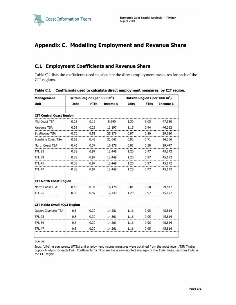
Coast Information Team
Economic Gain Spatial Analysis — Timber August 2004
Page C-1
Appendix C. Modelling Employment and Revenue Share
C.1 Employment Coefficients and Revenue Share
Table C.1 lists the coefficients used to calculate the direct employment measures for each of the CIT regions.
Table C.1 Coefficients used to calculate direct employment measures, by CIT region.
Management Within Region (per ‘000 m3) Outside Region ( per ‘000 m3)
Unit Jobs FTEs Income $ Jobs FTEs Income $
CIT Central Coast Region
Mid Coast TSA 0.28 0.19 8,590 1.30 1.05 47,530
Kincome TSA 0.39 0.28 13,197 1.15 0.94 44,312
Strathcona TSA 0.70 0.51 25,176 0.97 0.80 39,080
Sunshine Coast TSA 0.63 0.45 22,043 0.82 0.71 34,366
North Coast TSA 0.45 0.34 16,178 0.81 0.58 29,447
TFL 25 0.38 0.97 12,449 1.20 0.97 45,172
TFL 39 0.38 0.97 12,449 1.20 0.97 45,172
TFL 45 0.38 0.97 12,449 1.20 0.97 45,172
TFL 47 0.38 0.97 12,449 1.20 0.97 45,172
CIT North Coast Region
North Coast TSA 0.45 0.34 16,178 0.81 0.58 29,447
TFL 25 0.38 0.97 12,449 1.20 0.97 45,172
CIT Haida Gwaii /QCI Region
Queen Charlotte TSA 0.5 0.30 14,561 1.16 0.95 45,814
TFL 25 0.5 0.30 14,561 1.16 0.95 45,814
TFL 39 0.5 0.30 14,561 1.16 0.95 45,814
TFL 47 0.5 0.30 14,561 1.16 0.95 45,814
Source:
Jobs, full-time equivalents (FTEs) and employment income measures were obtained from the most recent TSR Timber Supply Analysis for each TSA. Coefficients for TFLs are the area-weighted averages of the TSAs measures from TSAs in the CIT region.
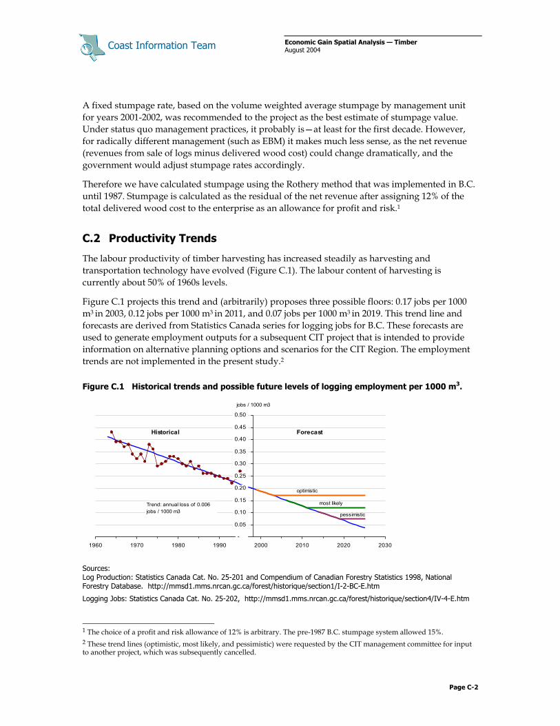
Coast Information Team
Economic Gain Spatial Analysis — Timber August 2004
Page C-2
A fixed stumpage rate, based on the volume weighted average stumpage by management unit for years 2001-2002, was recommended to the project as the best estimate of stumpage value. Under status quo management practices, it probably is—at least for the first decade. However, for radically different management (such as EBM) it makes much less sense, as the net revenue (revenues from sale of logs minus delivered wood cost) could change dramatically, and the government would adjust stumpage rates accordingly.
Therefore we have calculated stumpage using the Rothery method that was implemented in B.C. until 1987. Stumpage is calculated as the residual of the net revenue after assigning 12% of the total delivered wood cost to the enterprise as an allowance for profit and risk.1
C.2 Productivity Trends
The labour productivity of timber harvesting has increased steadily as harvesting and transportation technology have evolved (Figure C.1). The labour content of harvesting is currently about 50% of 1960s levels.
Figure C.1 projects this trend and (arbitrarily) proposes three possible floors: 0.17 jobs per 1000 m3 in 2003, 0.12 jobs per 1000 m3 in 2011, and 0.07 jobs per 1000 m3 in 2019. This trend line and forecasts are derived from Statistics Canada series for logging jobs for B.C. These forecasts are used to generate employment outputs for a subsequent CIT project that is intended to provide information on alternative planning options and scenarios for the CIT Region. The employment trends are not implemented in the present study.2
Figure C.1 Historical trends and possible future levels of logging employment per 1000 m3.
Sources: Log Production: Statistics Canada Cat. No. 25-201 and Compendium of Canadian Forestry Statistics 1998, National Forestry Database. http://mmsd1.mms.nrcan.gc.ca/forest/historique/section1/I-2-BC-E.htm
Logging Jobs: Statistics Canada Cat. No. 25-202, http://mmsd1.mms.nrcan.gc.ca/forest/historique/section4/IV-4-E.htm
1 The choice of a profit and risk allowance of 12% is arbitrary. The pre-1987 B.C. stumpage system allowed 15%. 2 These trend lines (optimistic, most likely, and pessimistic) were requested by the CIT management committee for input to another project, which was subsequently cancelled.
-
0.05
0.10
0.15
0.20
0.25
0.30
0.35
0.40
0.45
0.50
1960 1970 1980 1990 2000 2010 2020 2030
jobs / 1000 m3
Trend: annual loss of 0.006 jobs / 1000 m3 pessimistic
most likely
optimistic
Historical Forecast

Coast Information Team
Economic Gain Spatial Analysis — Timber August 2004
Page D-1
Appendix D. Specification of Scenarios
Table of Contents D.1 TSR Base Case Scenario...................................................................................................... 2 D.2 Financial Efficiency Scenario ................................................................................................ 3 D.3 Ecosystem-based Management Planning Handbook Scenarios ............................................... 4
D.3.1 Adjustments to Development Costs .......................................................................... 6 D.3.2 Ecosystem Surrogates.............................................................................................. 7 D.3.3 Range of Natural Variation ....................................................................................... 7 D.3.4 Regional-level Retention Constraint .......................................................................... 7 D.3.5 Landscape-level Retention Constraint ....................................................................... 7 D.3.6 Watershed-level Retention Constraint ....................................................................... 8 D.3.7 Mid-seral Constraint................................................................................................. 8 D.3.8 Stand-level Retention............................................................................................... 8 D.3.9 Red-listed Ecosystems Retention .............................................................................. 8
D.4 References ......................................................................................................................... 8
List of Tables
D.1 Timber supply analysis reports and management plans used in the development of the management assumptions of the TSR Base Case scenario..................................................... 2
D.2 Specifications of the TSR Base Case scenario. ...................................................................... 3
D.3 Specifications of the Financial Efficiency scenario.................................................................. 4
D.4 Specifications of the Ecosystem-based Management Planning Handbook (EBMPH) scenarios – common elements............................................................................................. 5
D.5 Constraint specifications of stand-level risk for Ecosystem-based Management Planning Handbook (EBMPH) scenarios.............................................................................................. 6
D.6 Development cost adjustment factors for EBM scenarios. ...................................................... 6
D.7 Site series (estimated) for ecosystem surrogates ( BEC variants x analysis units) for the CIT Region. .............................................................................................................................. 9
D.8 Subset of ecosystem surrogates comprising 95% of the productive forest area of the CIT Central Coast Region. ....................................................................................................... 10
D.9 Percent of forest land age 250+ years under natural disturbance regimes, CIT Region ......... 13
D.10 Percent of productive forest land that is red-listed, CIT Central Coast Region. ...................... 15

Coast Information Team
Economic Gain Spatial Analysis — Timber August 2004
Page D-2
The scenarios described in this appendix specify forest management objectives and operating conditions required to guide the execution of the forest model for analyses conducted in each of the three CIT regions—Central Coast, North Coast, and Haida Gwaii. Exceptions and special cases are noted for the Central Coast region scenarios.
These scenarios are not meant to represent actual policy options that might be implemented. They are analyzed with the intention of bounding the set of feasible policies and providing sufficient information to allow one to infer the effects on values derived from timber harvesting from subsequent intermediate policies that may be implemented.
D.1 TSR Base Case Scenario
The TSR Base Case scenario is a composite of the base case analyses undertaken in support of the Chief Forester’s annual harvest determination for each of the management units comprising the study area. The original individual analyses were intended to reflect current practices, and hence to represent a feasible policy.1 Here, it is included as a reference scenario representing the status quo policy and as a means of validation of our modelling methods.
The TSR Base Case scenarios developed for the CIT regions contains the management assumptions of the most recent TSR or MPs (including all harvest flow, disturbance, seral stage, and biodiversity constraints). The contributing reports are listed in Table D.1. Access to the management plans of the four tree farm licences was undertaken with the permission of the companies holding the licences.
Table D.2 describes the key components of the aggregate TSR Base Case scenarios.
Table D.1 Timber supply analysis reports and management plans used in the development of the management assumptions of the TSR Base Case scenario
Management unit Analysis document
1 Strathcona TSA Timber Supply Area Analysis Report, February 1999
2 Kingcome TSA Timber Supply Area Analysis Report, November 2001
3 Mid Coast TSA Timber Supply Area Analysis Report, June 1999
4 Sunshine Coast Timber Supply Area Analysis Report, June 2001
5 TFL 25 (Western) Management Plan No. 9 Timber Supply Analysis Report, 1996
6 TFL 39 (Weyerhaeuser) Management Plan No. 8 Timber Supply Analysis Report, March 2001
7 TFL 45 (Interfor) Management Plan No. 4 Timber Supply Analysis Report, September 2001
8 TFL 47 (TimberWest) Management Plan No. 3 Timber Supply Analysis Report, January 2002
9 North Coast TSA LRMP Timber Supply Analysis Report, October 2002
10 Queen Charlotte TSA Timber Supply Area Analysis Report, October 2000
1 “Policy” is used here in the modelling sense, as a set of decision values required to satisfy a model, as opposed to a policy implemented by government.

Coast Information Team
Economic Gain Spatial Analysis — Timber August 2004
Page D-3
Table D.2 Specifications of the TSR Base Case scenario
Component Description
1 Management objective Maximize harvest volume (given the conditions and constraints listed below)
2 Costs model Base case cost model (see Appendix B)
3 Price model 4 price assumptions relative to the top-to-trough price cycle amplitude: 25%, 50%, 75%, 100% (see Appendix B)
4 Operability Harvest if m3/ha > 350a
5 Harvest flow constraints As per Base Case of each TSA or TFL
6 Timber lease conversions As per Base Case of each TSA or TFL
7 IRM green-up (disturbance) constraints
As per Base Case of each TSA or TFL
8 VQO green-up (disturbance) constraints
As per Base Case of each TSA or TFL
9 Community watershed constraints As per Base Case of each TSA or TFL
10 Ungulate range constraints As per Base Case of each TSA or TFL
11 Grizzly habitat constraints As per Base Case of each TSA or TFL
12 Retention constraints As per Base Case of each TSA or TFL
a Stands are eligible for harvesting when the operability condition is met – minimum harvest ages are not specified in the model.
Note: Riparian and terrain constraints are represented by inclusion factors (% netdowns) in the TSR landbase used in all of the scenarios in this study.
D.2 Financial Efficiency Scenario
The Financial Efficiency scenario, summarized in Table D.3, differs from the Base Case scenario in three ways.
1. The management objective for the Central Coast LRMP area, the North Coast and Haida Gwaii regions is to maximize the net present value (NPV) at 5%, i.e., to schedule timber harvest such that the future stream of net revenue from that harvest, discounted at a rate of 5% annually, is maximized. The management objective for the remainder of the CIT Central Coast region is to maximize the volume harvested.2
2. The total harvest volume from the Central Coast LRMP area must be even flow, meaning that it cannot decrease or increase over the 200-year planning period. The harvest flow from the remainder of the CIT Central Coast region, as well as the North Coast and Haida Gwaii regions, is also required to be even flow.
3. For a stand within the THLB to be harvestable, it must yield at least 350 m3 and must yield positive net revenue. The latter condition may seem redundant given that the model is driven by the objective of maximizing NPV. However, the requirement for even-flow harvest may make it attractive to harvest some stands at a loss, to maintain the even-flow harvest at the highest possible rate.
2 Timber harvesting cost and value information was available for the LRMP area only.

Coast Information Team
Economic Gain Spatial Analysis — Timber August 2004
Page D-4
Table D.3 Specifications of the Financial Efficiency scenario
Component Description
1 Management objective For the Central Coast (CC) region, maximize the net present value of the harvest on the LRMP area, and maximize volume harvested on the remainder of the CC region, given the conditions and constraints listed below For the North Coast (NC) and Haida Gwaii (HG) regions, maximize the net present value
2 Cost model Base case cost model (see Appendix B)a
3 Price model Top-of-the-cycle prices (see Appendix B)b
4 Operability For the CC region, on the LRMP area harvest if m3/ha > 350 AND net revenue > 0; on the remaining CC region, harvest if m3/ha > 350 For the NC and HG regions, area harvest if m3/ha > 350 AND net revenue > 0
5 Harvest flow constraints For the CC region, even flow within the LRMP area and also even flow in the remainder of the CC region For the NC and HG regions, even flow
6 Timber lease conversions As per Base Case of each TSA or TFL
7 IRM green-up (disturbance) constraints
As per Base Case of each TSA or TFL
8 VQO green-up (disturbance) constraints
As per Base Case of each TSA or TFL
9 Community watershed constraints As per Base Case of each TSA or TFL
10 Ungulate range constraints As per Base Case of each TSA or TFL
11 Grizzly habitat constraints As per Base Case of each TSA or TFL
12 Retention constraints As per Base Case of each TSA or TFL
a Costs were used in the calculation of net revenue but are not reported here b The price model calculates four prices relative to the top-to-trough price-cycle amplitude: 25%, 50%, 75%, 100% (see Appendix B). Only top-of-the-cycle prices were used to obtain the results reported here.
D.3 Ecosystem-based Management Planning Handbook Scenarios
Three scenarios are included that represent a range of policy options under EBM management, as developed in the Ecosystem-based Management Planning Handbook (EBMPH). These scenarios are intended to provide information on the implications of alternative policy choices.
The EBMPH scenarios all model low environmental risk (or less) at the subregional level and intermediate risk (or less) at the landscape level. The three scenarios differ in that they model low, intermediate, and high levels of risk at the stand level. The watershed level of risk recognized in the handbook was not modelled in the Central Coast analysis as the appropriate watershed coverage was not included in the study’s landbase data set.
The low end of the EBMPH envelope would therefore be more restrictive than the low risk scenario represented in this study, e.g., a decision to use low risk as the target at all levels would involve lowering landscape-level risk from intermediate to low, and lowering watershed-level risk from high to low, while subregional- and stand-level risk would remain unchanged at low. The EBMPH Low Stand-Level Risk scenario as modelled in this report is not equivalent to the
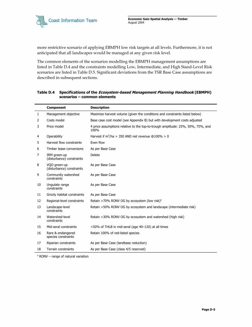
Coast Information Team
Economic Gain Spatial Analysis — Timber August 2004
Page D-5
more restrictive scenario of applying EBMPH low risk targets at all levels. Furthermore, it is not anticipated that all landscapes would be managed at any given risk level.
The common elements of the scenarios modelling the EBMPH management assumptions are listed in Table D.4 and the constraints modelling Low, Intermediate, and High Stand-Level Risk scenarios are listed in Table D.5. Significant deviations from the TSR Base Case assumptions are described in subsequent sections.
Table D.4 Specifications of the Ecosystem-based Management Planning Handbook (EBMPH) scenarios – common elements
Component Description
1 Management objective Maximize harvest volume (given the conditions and constraints listed below)
2 Costs model Base case cost model (see Appendix B) but with development costs adjusted
3 Price model 4 price assumptions relative to the top-to-trough amplitude: 25%, 50%, 75%, and 100%
4 Operability Harvest if m3/ha > 350 AND net revenue @100% > 0
5 Harvest flow constraints Even flow
6 Timber lease conversions As per Base Case
7 IRM green-up (disturbance) constraints
Delete
8 VQO green-up (disturbance) constraints
As per Base Case
9 Community watershed constraints
As per Base Case
10 Ungulate range constraints
As per Base Case
11 Grizzly habitat constraints As per Base Case
12 Regional-level constraints Retain >70% RONV OG by ecosystem (low risk)a
13 Landscape-level constraints
Retain >50% RONV OG by ecosystem and landscape (intermediate risk)
14 Watershed-level constraints
Retain >30% RONV OG by ecosystem and watershed (high risk)
15 Mid-seral constraints <50% of THLB in mid-seral (age 40–120) at all times
16 Rare & endangered species constraints
Retain 100% of red-listed species
17 Riparian constraints As per Base Case (landbase reduction)
18 Terrain constraints As per Base Case (class 4/5 reserved)
a RONV – range of natural variation

Coast Information Team
Economic Gain Spatial Analysis — Timber August 2004
Page D-6
Table D.5 Constraint specifications of stand-level risk for Ecosystem-based Management Planning Handbook (EBMPH) scenarios
EBMPH stand-level risk scenarios
% RONV old growth retained by ecosystem type
Low 70%
Intermediate 45%
High 15%
D.3.1 Adjustments to Development Costs
The costs of developing roads and bridges are termed “development” costs in the Coast Appraisal Manual and are allocated over the tributary volume—usually the estimated volume from the next cutting authority—on a unit basis ($/m3). The woodshed studies, which are the source of wood cost data for this study, estimated total development costs for contiguous areas (woodsheds) serviced by a single gathering point (or multiple, closely related points), and allocated these costs across the operable volume of mature timber within the woodshed.
This study assumes that the operable volume of timber in each woodshed was determined in a manner consistent with the TSR Base Case scenario. To the extent that EBMPH results in reduced harvest levels, we expect that development costs estimated for a woodshed will be amortized over a smaller harvest volume under EBMPH scenarios.
The development cost for each woodshed is adjusted by multiplying the original costs obtained from the woodshed study by the inverse of the proportion harvested under the stand-level retention constraints. This calculation assumes that 100% of the woodshed would be harvested under the TSR Base Case and that the area harvested under an EBMPH scenario could not exceed the proportion harvestable under the stand-level retention constraint. These adjustment factors are listed in Table D.6.
Table D.6 Development cost adjustment factors for EBM scenarios
EBM scenario Proportion of stand available for harvest
Development cost adjustment factor
Low Risk 0.30 3.33
Intermediate Risk 0.55 1.81
High Risk 0.85 1.18
The adjustment factors may be modified if information is available indicating that development costs may be reduced in specific woodsheds under EBMPH, e.g., if fewer roads were to be

Coast Information Team
Economic Gain Spatial Analysis — Timber August 2004
Page D-7
constructed. If the reduction in harvest exceeds the stand-level harvest proportion, then the cost factors may be adjusted further. 3
D.3.2 Ecosystem Surrogates
The EBM retention constraints were intended to be applied by ecosystem, but BEC site series—typically used to identify “ecosystems” at the scale of this study—were unavailable. Therefore, intersections of BEC variant x analysis unit were used as surrogates of ecosystems, following Holt and Sutherland (2003). Table D.7 lists the site series or groups of site series likely associated with each BEC variant and analysis unit across the entire CIT Analysis Area (Central Coast, North Coast, and Haida Gwaii).
Of the 330 potential ecosystem surrogates in Table D.7, 256 have area in the CIT Central Coast Region, and only 75 of these account for 95% of the total productive forest area. Similarly, 28 and 24 ecosystem surrogates account for 95% of the productive forest area of the North Coast and Haida Gwaii regions, respectively. These subsets of ecosystem surrogates were incorporated in the model to track violations of retention constraints. Table D.8 lists the subsets of the ecosystem surrogates.
D.3.3 Range of Natural Variation
The regional-, landscape-, and watershed-level EBMPH constraints specify retention of old forest (age 250+) by ecosystem surrogate, as a percentage of the expected area of old forest under natural disturbance regimes. Estimates of area by age class were supplied to this project as BEC variant x analysis unit disturbance units, and used to populate Table D.9.4 Of the 17 disturbance units (sets of BEC variants and analysis units), five sets accounted for 95% of the productive forest area of the CIT Central Coast Region, and were represented explicitly in the model. The remaining units were aggregated and assigned an area-weighted average percent of old forest. The same approach was taken for the North Coast and Haida Gwaii regions.
D.3.4 Regional-level Retention Constraint
The regional-level retention constraint requires that a percentage of each ecosystem in the region be at least 250 years of age. The percentage is the product of a specified retention level and the percentage of forest land aged 250+ expected under natural disturbance regimes (from Table D.9). The retention level required by the EBMPH scenarios is 70%.
Note that the LRMP portion of the CIT Central Coast Region presently is in violation of the regional-level retention constraints: 9.7% of the productive forest landbase does not meet the constraint before modelling additional harvesting.
D.3.5 Landscape-level Retention Constraint
The landscape-level retention constraint requires that a percentage of each ecosystem on each landscape (CIT landscape/seascape) be at least 250 years of age. The percentage is the product of 3 Development costs were adjusted subsequent to preliminary runs for the Central Coast analysis and are described in the Scenario Analysis section of this report. 4 The author (K. Price) expressed unease with providing these estimates by BEC variant and analysis unit, contending that disturbance units based on physiographic region and site series was a superior approach.

Coast Information Team
Economic Gain Spatial Analysis — Timber August 2004
Page D-8
a specified retention level and the percentage of forest land aged 250+ expected under natural disturbance regimes (from Table D.6). The retention level required by the EBMPH scenarios is 50%.
Presently, the LRMP portion of the CIT Central Coast Region is in violation of the landscape-level retention constraints: 4.5% of the productive forest landbase does not meet the constraints.
D.3.6 Watershed-level Retention Constraint
The watershed-level retention constraint requires that a percentage of each ecosystem on each watershed be at least 250 years of age. The percentage is the product of a specified retention level and the percentage of forest land aged 250+ expected under natural disturbance regimes (from Table D.9). The retention level required for the EBM scenarios is 30%.
The watershed–level retention constraint was not applied in the CIT Central Coast region scenario analysis as the necessary watershed coverage was not included in the data set developed for this study.
D.3.7 Mid-seral Constraint
The mid-seral constraint requires that less than 50% of the timber harvesting landbase within each ecosystem be age 40–120 years. Currently less than 1% of the landbase is in violation of this constraint.
D.3.8 Stand-level Retention
Stand-level retention is modelled by converting a portion of each development type (inventory strata) scheduled for harvest to “retained” status at the time of the first modelled harvest. The retention rate is 70%, 45%, and 15% for High, Intermediate, and Low Stand-Level Risk scenarios, respectively.
D.3.9 Red-listed Ecosystems Retention
Red-listed ecosystems—ecosystems that are extirpated, endangered, or threatened in British Columbia—are 100% retained in the EBM scenarios evaluated in this study. Table D.10 lists the percentages of each ecosystem surrogate estimated to be red listed in the CIT regions.
Applying these estimates, we calculated that 4.7% of the productive forest landbase of the Central Coast region is red listed. Red-listed ecosystems occurring in the timber harvesting landbase were converted to an “inoperable” state that cannot be harvested.
The forest area red listed on the North Coast is small—about 300 ha—and the area red listed on Haida Gwaii is 6,313 ha or 2.5% of the THLB. However, in both of these regions the red listed ecosystems are valuable stands—good site spruce on CWHvh2 and CWHwh1.
D.4 References
Holt, R.F. and G. Sutherland. 2003. Environmental risk assessment: Base case—Coarse filter biodiversity. Unpublished report prepared for the North Coast LRMP.

Coast Information Team
Economic Gain Spatial Analysis — Timber August 2004
Page D-9
Table D.7 Site series (estimated) for ecosystem surrogates ( BEC variants x analysis units) for the CIT Region. (A. Banner, pers. comm.)
1: Fir 2: Fir 3: Fir 4: Cedar 5: Cedar 6: Cedar 7: HemBal 8: HemBal 9: HemBal 10: Spr Pine 11: Spr Pine 12: Spr PineITG 1-8 ITG 1-8 ITG=1-8 ITG=9-11 ITG=9-11 ITG=9-11 ITG=12-20 ITG=12-20 ITG=12-20 ITG=21-34 ITG=21-34 ITG=21-34
BEC Good Medium Poor Good Medium Poor Good Medium Poor Good Medium Poor
ATCWHdm 05, 07 01, 04, (06) 02, 03 05, 07 01, 04, 06 11, 12, 02, 03 05, 07 01, 04, (06) 03 08 08 12CWHds2 05, 07 01, 04, (06) 02, 03 05, 07 01, 06 02, 03, 12 05, 07 01, 06 03 08 08 12CWHmm1 05, 07 01, (06, 04) 02, 03 05, 07 01, (04, 06) 12, 03 05, 07 01, 04, (06) 03 08?, 08?, 12CWHmm2 05,08 01, 06 04, 02, 03 (05, 08) 01, (04) 07, (10) 05, 08 01, (06) 03, (07)CWHms2 04, 06 01, 05 02, 03 04, 06 01, 05 11, (03) 04, 06 01, 05 03 07, 07, 11,CWHvh1CWHvh2 06, 07, (05) 04, (13) 01, 03, 11 06, 07, (05) 04 04 08, (09) 06, 07, (05), (15, 17)a 13, (18, 19), (14, 16)a
CWHvm 05, 08 01, 06, (04) 06, CWHvm1 05, 08 (04), 01, 06, (14) 12, 03, (02) 05, 08 (04), 01, 06 6 09, (08) 05, 08 14CWHvm2 05, 08 01, 06, (04) 06, (01) 05, 08c 01, 06, (04, 11)c 09, 03, (02)c 05, 08c 01, 06, (04)c 06, (01)c (08)c 05, 08c 11c
CWHvm3CWHwh
CWHwmd 04 04, 03 08, 02 04 01, 03 08, 02 05, (04) 03 09CWHws2 06, 01, 04, 05 03, 05 06e 01, 04, (05)e 03, 05e 06e 01, 04, 05e 03, 05e 07, (06)e 04, (06)e 11e
CWHxm 05, 07 01, 04, 06 02, 03 05, 07 01, 04, 06, 13 (03), 12 05, 07 01, 04, 06 03, (12) 08 08 12, 13CWHxm1CWHxm2ESSFmcESSFmkESSFmwESSFmwhIDFwwMHmm1 (05) 01, 05, 03 02, 04, 06, 07, 08, 09 (04, 05)f 01, 03, 05 02, 04, 06, 07, 08, 09 N/Af N/Af N/Af
MHmm2MHmm2e
MHmmp MHwhg (05) 01, 05 02, 04, 06, 07, 08, 09 05f 01, 05 02, 04, 06,07,08,09 N/Af N/Af N/Af
MHwh1not classified
Brackets () around site series denote that the site series is either restricted in distribution or less commonly associated with the analysis unit.Footnotes:
a Shorline Forestsb Brackish Water (Estuaries)c Higher elevations; productivity declines; yellow cedar replaces redcedard Redcedar and Balsam uncommon in CWHwme Includes CWHws1 and ws2f This analysis unit probably does not occur in the MH zoneg Yellow-cedar and Mountain Hemlock replace Red-cedar and Western Hemlock in the MH zone

Coast Information Team
Economic Gain Spatial Analysis — Timber August 2004
Page D-10
Table D.8 Subset of ecosystem surrogates comprising 95% of the productive forest area by CIT region.
CIT Central Coast Region
BEC variant Analysis unit Area % cumulative 1 CWHvh2 6: Cedar SI <=15 242,202 12% 2 CWHvm1 8: HemBal 12.6<= SI <=22 142,905 20% 3 CWHvm1 6: Cedar SI <=15 136,727 26% 4 CWHvm1 7: HemBal SI >22 125,637 33% 5 CWHvh1 6: Cedar SI <=15 124,363 39% 6 CWHvm1 5: Cedar 16<= SI <=23 82,386 43% 7 CWHvm2 6: Cedar SI <=15 81,713 47% 8 CWHms2 8: HemBal 12.6<= SI <=22 59,196 50% 9 CWHvm2 8: HemBal 12.6<= SI <=22 57,120 53%
10 CWHws2 8: HemBal 12.6<= SI <=22 53,087 56% 11 CWHvh2 5: Cedar 16<= SI <=23 44,737 58% 12 CWHvm2 9: HemBal SI <=12.5 42,617 60% 13 MHmm2 9: HemBal SI <=12.5 39,925 63% 14 CWHvh2 8: HemBal 12.6<= SI <=22 38,370 64% 15 MHmm1 9: HemBal SI <=12.5 36,320 66% 16 CWHws2 9: HemBal SI <=12.5 32,363 68% 17 CWHvm1 9: HemBal SI <=12.5 28,746 69% 18 CWHvm1 13: Decid SI = all 22,747 71% 19 CWHvh2 9: HemBal SI <=12.5 21,927 72% 20 CWHvh2 7: HemBal SI >22 20,861 73% 21 CWHvh1 8: HemBal 12.6<= SI <=22 20,815 74% 22 CWHvm3 8: HemBal 12.6<= SI <=22 20,142 75% 23 CWHxm2 7: HemBal SI >22 18,048 76% 24 CWHxm2 1: Fir SI>27 18,042 77% 25 CWHvh1 5: Cedar 16<= SI <=23 15,751 77% 26 CWHvm2 5: Cedar 16<= SI <=23 15,612 78% 27 MHmm1 6: Cedar SI <=15 15,457 79% 28 MHmm2 8: HemBal 12.6<= SI <=22 15,241 80% 29 CWHxm2 2: Fir 21<= SI <=27 13,928 80% 30 CWHvm3 9: HemBal SI <=12.5 13,699 81% 31 MHmm1 8: HemBal 12.6<= SI <=22 13,394 82% 32 CWHms2 9: HemBal SI <=12.5 12,182 82% 33 CWHvm2 7: HemBal SI >22 11,335 83% 34 CWHmm1 8: HemBal 12.6<= SI <=22 10,957 84% 35 CWHvm1 4: Cedar SI >23 10,443 84% 36 CWHvh1 7: HemBal SI >22 9,975 85% 37 CWHds2 8: HemBal 12.6<= SI <=22 9,881 85% 38 CWHms2 2: Fir 21<= SI <=27 8,377 86% 39 CWHvh1 9: HemBal SI <=12.5 8,266 86% 40 CWHvm1 2: Fir 21<= SI <=27 8,189 86% 41 CWHms2 13: Decid SI = all 7,567 87% 42 CWHms2 7: HemBal SI >22 7,392 87% 43 CWHxm2 8: HemBal 12.6<= SI <=22 7,316 88% 44 CWHms2 3: Fir SI <=20 7,111 88% 45 CWHds2 3: Fir SI <=20 6,908 88% 46 CWHxm1 1: Fir SI>27 6,776 89% 47 CWHdm 7: HemBal SI >22 6,718 89% 48 CWHvm1 10: Spr Pine SI >22 6,371 89% 49 CWHvm1 11: Spr Pine 16<= SI <=22 6,235 90% 50 CWHms2 5: Cedar 16<= SI <=23 6,165 90% 51 CWHds2 2: Fir 21<= SI <=27 5,928 90% 52 CWHxm2 3: Fir SI <=20 5,921 90% 53 ZZZZ 9: HemBal SI <=12.5 5,895 91% 54 CWHds2 12: Spr Pine SI <15 5,869 91% 55 CWHvm 6: Cedar SI <=15 5,852 91% 56 CWHvm1 1: Fir SI>27 5,400 92% 57 CWHvm 8: HemBal 12.6<= SI <=22 4,727 92% 58 CWHmm1 7: HemBal SI >22 4,629 92%

Coast Information Team
Economic Gain Spatial Analysis — Timber August 2004
Page D-11
Table D.8 (Continued)
BEC variant Analysis unit Area % Cumulative 59 CWHvh1 4: Cedar SI >23 4,418 92% 60 ZZZZ 6: Cedar SI <=15 4,390 93% 61 CWHvm1 12: Spr Pine SI <15 4,010 93% 62 CWHms2 6: Cedar SI <=15 3,896 93% 63 CWHmm2 8: HemBal 12.6<= SI <=22 3,859 93% 64 CWHws2 3: Fir SI <=20 3,812 93% 65 CWHds2 9: HemBal SI <=12.5 3,578 94% 66 CWHws2 12: Spr Pine SI <15 3,513 94% 67 CWHvh2 13: Decid SI = all 3,355 93.9% 68 CWHvm 9: HemBal SI <=12.5 3,025 94.1% 69 CWHxm2 13: Decid SI = all 3,006 94.2% 70 CWHvm1 3: Fir SI <=20 3,001 94.4% 71 CWHvh2 12: Spr Pine SI <15 2,813 94.5% 72 CWHds2 13: Decid SI = all 2,700 94.6% 73 MHwh1 6: Cedar SI <=15 2,653 94.8% 74 IDFww 12: Spr Pine SI <15 2,557 94.9% 75 CWHvh1 11: Spr Pine 16<= SI <=22 2,452 95.0%
CIT North Coast Region
BEC Variant Analysis Unit Area % Cumulative1 CWHvh2 3: Cedar SI < 15 290,090 36%2 CWHvh2 13: Cedar, fir All 61,860 43%3 CWHvm 3: Cedar SI < 15 58,906 51%4 CWHvm 8: Hemlock SI < 15 54,760 57%5 CWHwm 3: Cedar SI < 15 34,003 62%6 CWHvh2 8: Hemlock SI < 15 32,726 66%7 CWHwm 8: Hemlock SI < 15 28,413 69%8 MHmm1 8: Hemlock SI < 15 27,414 73%9 MHwh 3: Cedar SI < 15 23,941 75%
10 CWHvm 6: Hemlock SI 15-22 17,886 78%11 CWHvh2 14: Pine All 16,978 80%12 MHmm1 3: Cedar SI < 15 14,064 82%13 CWHvh2 6: Hemlock SI 15-22 12,628 83%14 CWHvh2 2: Cedar SI 15-22 12,465 85%15 CWHvm1 3: Cedar SI < 15 10,767 86%16 MHwh 8: Hemlock SI < 15 10,500 87%17 MHmm2 8: Hemlock SI < 15 9,191 88%18 CWHws2 8: Hemlock SI < 15 7,414 89%19 CWHvm1 4: Hemlock SI > 22 6,852 90%20 CWHwm 6: Hemlock SI 15-22 6,455 91%21 CWHvm2 3: Cedar SI < 15 5,361 92%22 CWHvm 4: Hemlock SI > 22 4,932 92%23 CWHvm1 6: Hemlock SI 15-22 4,210 93%24 CWHvm2 8: Hemlock SI < 15 4,046 93%25 CWHvm 2: Cedar SI 15-22 3,792 94%26 CWHvm 10: Spruce SI 15-22 3,714 94%27 CWHvh2 11: Spruce SI < 15 3,411 95%28 GROUP Group Group 44,241 100%

Coast Information Team
Economic Gain Spatial Analysis — Timber August 2004
Page D-12
Table D.8 (Continued)
CIT Haida Gwaii Region
BEC Variant Analysis Unit Area % Cumulative1 CWHwh1 3: Cedar SI < 12.5 108,578 18%2 CWHwh1 4: Hemlock SI >= 18 90,342 32%3 CWHvh2 3: Cedar SI < 12.5 58,048 42%4 CWHwh1 1: Cedar SI >= 15 48,252 49%5 CWHvh2 6: Hemlock SI < 15 43,234 56%6 CWHwh1 7: Spruce SI >= 16 37,759 63%7 CWHwh1 2: Cedar 12.5 <= SI < 15 25,020 67%8 CWHwh1 6: Hemlock SI < 15 23,075 70%9 CWHwh2 4: Hemlock SI >= 18 18,987 73%
10 CWHwh1 5: Hemlock 15 <= SI < 18 14,420 76%11 CWHvh2 5: Hemlock 15 <= SI < 18 13,470 78%12 CWHvh2 4: Hemlock SI >= 18 11,575 80%13 CWHwh2 3: Cedar SI < 12.5 10,899 82%14 CWHwh2 6: Hemlock SI < 15 10,657 83%15 CWHvh2 8: Spruce SI < 16 9,618 85%16 CWHwh2 5: Hemlock 15 <= SI < 18 9,090 86%17 CWHvh2 7: Spruce SI >= 16 8,856 88%18 CWHwh2 1: Cedar SI >= 15 7,942 89%19 CWHvh2 2: Cedar 12.5 <= SI < 15 7,492 90%20 CWHwh1 8: Spruce SI < 16 7,081 91%21 CWHwh1 9: Pine All SI 6,809 92%22 CWHvh2 1: Cedar SI >= 15 6,407 93%23 CWHwh1 10: Deciduous All SI 5,845 94%24 MHwh1 6: Hemlock SI < 15 4,188 95%

Coast Information Team
Economic Gain Spatial Analysis — Timber August 2004
Page D-13
Table D.9 Percent of forest land age 250+ years under natural disturbance regimes, by CIT region (K. Price, pers. comm.)
CIT Central Coast Region
1: Fir 2: Fir 3: Fir 4: Cedar 5: Cedar 6: Cedar 7: HemBal 8: HemBal 9: HemBal 10: Spr Pine 11: Spr Pine 12: Spr Pine 13: DecidITG 1-8 ITG 1-8 ITG=1-8 ITG=9-11 ITG=9-11 ITG=9-11 ITG=12-20 ITG=12-20 ITG=12-20 ITG=21-34 ITG=21-34 ITG=21-34 ITG=35-42
BEC SI>27 21<= SI <=27 SI <=20 SI >23 16<= SI <=23 SI <=15 SI >22 12.6<= SI <=22 SI <=12.5 SI >22 16<= SI <=22 SI <15 SI = all
ATCWHdm 73 48 48 73 73 86 73 73 73 86 86CWHds2 50 50 68 68 68 85 85 85 85 85 99CWHmm1 73 48 48 73 73 86 73 73 73 86 86CWHmm2 73 48 48 73 73 86 73 73 73 86 86CWHms2 73 48 48 73 73 86 73 73 73 86 86CWHvh1 90 97 97 83 97 97 83 83 97CWHvh2 90 97 97 83 97 97 83 83 97CWHvm 65 83 93 93 83 83 83 83 83 93CWHvm1 65 83 93 93 83 83 83 83 83 93CWHvm2 65 83 93 93 83 83 83 83 83 93CWHvm3 65 83 93 93 83 83 83 83 83 93CWHws2 50 50 68 68 68 85 85 85 85 85 99CWHxm 73 48 48 73 73 86 73 73 73 86 86CWHxm1 73 48 48 73 73 86 73 73 73 86 86CWHxm2 73 48 48 73 73 86 73 73 73 86 86ESSFmcESSFmkESSFmw 50 50 68 68 68 85 85 85 85 85 99ESSFmwhIDFww 50 50 68 68 68 85 85 85 85 85 99MHmm1 83 93 93 83 83 83 83 83 93MHmm2 83 93 93 83 83 83 83 83 93MHmm2e 83 93 93 83 83 83 83 83 93MHmmp 83 93 93 83 83 83 83 83 93MHwh 90 97 97 83 97 97 83 83 97MHwh1 90 97 97 83 97 97 83 83 97not classified

Coast Information Team
Economic Gain Spatial Analysis — Timber August 2004
Page D-14
Table D.9 (Continued)
CIT North Coast Region
CIT Haida Gwaii Region
Cedar Cedar Cedar Hemlock Hemlock b Hemlock Hemlock b Hemlock Spruce Spruce Spruce Cottonwood Cedar, fir PineITG 9,11,14 ITG ITG ITGa ITGa ITGa ITGa ITGa ITG 21,23,24,26 ITG 21,23,24,26 ITG 21,23,24,26 ITG 35,36 ITG 10 ITG 27-33
BEC SI > 22 SI 15-22 SI < 15 SI > 22 SI > 22 SI 15-22 SI 15-22 SI < 15 SI > 22 SI 15-22 SI < 15 All All All
ATCWHvh2 97 97 97 97 97 97 100CWHvm 93 93 83 83 83 83CWHvm1 93 83 83CWHvm2 93 83CWHwm 88 88 88CWHws1CWHws2 85MHmm1 93 83MHmm2 83MHwh 97 97
a ITG - 12,15,16,17,18,19,20,37b thinned stands
1: Cedar 2: Cedar 3: Cedar 4: Hemlock 5: Hemlock 6: Hemlock 7: Spruce 8: Spruce 9: Pine 10: DeciduousITG=9-11 ITG=9-11 ITG=9-11 ITG=12-20 ITG=12-20 ITG=12-20 ITG=21-26 ITG=21-26 ITG=28-30 ITG=37,38
BEC SI >= 15 12.5<= SI <15 SI < 12.5 SI >= 18 15 <= SI < 18 SI < 15 SI >= 16 SI < 16 All SI All SI
AT 100 52 34 100 75 26CWHvh2 91 83 83 34 81 80 41 79 52 1CWHwh1 68 75 94 22 88 71 17 86 11 0CWHwh2 96 91 89 43 95 89 33 95 95MHwh 100 94 48 84 91 90 64 63MHwh1 100 95 80 33 91 88 84 91 42MHwh2 100 100 95 17 97 85 59 99
not classified 84 86 66 4 66 70 15 66

Coast Information Team
Economic Gain Spatial Analysis — Timber August 2004
Page D-15
Table D.10 Percent of productive forest land that is red listed, CIT Central Coast Region (A. Banner, pers. comm.)
1: Fir 2: Fir 3: Fir 4: Cedar 5: Cedar 6: Cedar 7: HemBal 8: HemBal 9: HemBal 10: Spr Pine 11: Spr Pine 12: Spr Pine 13: DecidITG 1-8 ITG 1-8 ITG=1-8 ITG=9-11 ITG=9-11 ITG=9-11 ITG=12-20 ITG=12-20 ITG=12-20 ITG=21-34 ITG=21-34 ITG=21-34 ITG=35-42
BEC SI>27 21<= SI <=27 SI <=20 SI >23 16<= SI <=23 SI <=15 SI >22 12.6<= SI <=22 SI <=12.5 SI >22 16<= SI <=22 SI <15 SI = all
ATCWHdm 10 20 20 10 20 20 10 20 100 100 10CWHds2 100 100 10 100 100 10 100 100 100 100 10CWHmm1 100 10 80 100 10 20 100 10 100 100 100 10CWHmm2 10 50 10CWHms2 100 100 20CWHvh1 100CWHvh2 100CWHvm 70CWHvm1 70CWHvm2CWHvm3CWHws2 80CWHxm 50 100 20 50 100 50 100 100 100 20 10CWHxm1 50 100 20 50 100 50 100 100 100 20 10CWHxm2 50 100 20 50 100 50 100 100 100 20 10ESSFmc `ESSFmkESSFmwESSFmwhIDFwwMHmm1MHmm2MHmm2eMHmmpMHwh MHwh1not classified