Coalgebraic weak bisimulation for action-type systems

Sokolova, A.; de Vink, E.P.; Woracek, H.

Published in:Scientific Annals of Computer Science

DOI:10.1007/BF01287580

Published: 01/01/2009

Document VersionPublisher’s PDF, also known as Version of Record (includes final page, issue and volume numbers)

Please check the document version of this publication:

• A submitted manuscript is the author's version of the article upon submission and before peer-review. There can be important differencesbetween the submitted version and the official published version of record. People interested in the research are advised to contact theauthor for the final version of the publication, or visit the DOI to the publisher's website.• The final author version and the galley proof are versions of the publication after peer review.• The final published version features the final layout of the paper including the volume, issue and page numbers.

Link to publication

Citation for published version (APA):Sokolova, A., Vink, de, E. P., & Woracek, H. (2009). Coalgebraic weak bisimulation for action-type systems.Scientific Annals of Computer Science, 19, 93-144. DOI: 10.1007/BF01287580

General rightsCopyright and moral rights for the publications made accessible in the public portal are retained by the authors and/or other copyright ownersand it is a condition of accessing publications that users recognise and abide by the legal requirements associated with these rights.

• Users may download and print one copy of any publication from the public portal for the purpose of private study or research. • You may not further distribute the material or use it for any profit-making activity or commercial gain • You may freely distribute the URL identifying the publication in the public portal ?

Take down policyIf you believe that this document breaches copyright please contact us providing details, and we will remove access to the work immediatelyand investigate your claim.

Download date: 02. May. 2018

Scientific Annals of Computer Science vol. 19, 2009

“Alexandru Ioan Cuza” University of Iasi, Romania

Coalgebraic Weak Bisimulation

for Action-Type Systems

Ana SOKOLOVA1, Erik de VINK2, Harald WORACEK3

Abstract

We propose a coalgebraic definition of weak bisimulation for classes ofcoalgebras obtained from bifunctors in the category Set. Weak bisim-ilarity for a system is obtained as strong bisimilarity of a transformedsystem. The particular transformation consists of two steps: First, thebehavior on actions is lifted to behavior on finite words. Second, thebehavior on finite words is taken modulo the hiding of internal or in-visible actions, yielding behavior on equivalence classes of words closedunder silent steps. The coalgebraic definition is validated by two cor-respondence results: one for the classical notion of weak bisimulationof Milner, another for the notion of weak bisimulation for generativeprobabilistic transition systems as advocated by Baier and Hermanns.

1 Introduction

We present a definition of weak bisimulation for action type systems basedon the general coalgebraic apparatus of bisimulation [1, 21, 38]. Action-typesystems are systems that arise from bifunctors in the category Set. A typicaland familiar example of an action-type system is a labelled transition system

1Department of Computer Sciences, Universitat Salzburg, Jakob-Haringer-Str. 2, 5020Salzburg, Austria, Email: anas@cs.uni-salzburg.at, supported by the Austrian ScienceFunds (FWF) P18913- N15 and V00125

2Department of Mathematics and Computer Science, Technische Universiteit Eind-hoven, P.O. Box 513, 5600 MB Eindhoven, the Netherlands, Email: evink@win.tue.nl

3Institute for Analysis and Scientific Computing, Technische Universitat Wien, Wied-ner Haupstr. 8–10, 1040 Wien, Austria, Email: harald.woracek@tuwien.ac.at

93

(LTS) (see, e.g., [22, 33]), but also many types of probabilistic systems (see,e.g., [24, 40, 17, 7, 39]) fall into this class. Informally, an action-type systemin Set is a coalgebra that performs actions from a set A.

For the verification of system properties, behavior equivalences are of-ten employed. One such behavior equivalence is strong bisimilarity. How-ever strong bisimilarity is often too strong an equivalence. Weak bisimilar-ity, originally defined for LTSs in the work of Milner [28, 30], is a looserequivalence on systems that abstracts away from internal or invisible steps.In fact, weak bisimilarity for a labelled transition system S amounts tostrong bisimilarity on the ‘double-arrowed’ system S ′ induced by S. In fact,the ‘double-arrowed’ system is the original system saturated with invisiblesteps. We generalize this idea for a coalgebraic definition of weak bisimula-tion. Our approach, given a system S, consists of two stages.

1. First, we define a ‘∗-extension’ S ′ of S which is a system with thesame carrier as S, but with action set A∗, the set of all finite wordsover A. The system S ′ captures the behavior of S on finite traces.

2. Next, given a set of invisible actions τ ⊆ A, we transform S ′ into aso-called ‘weak τ -extension’ S ′′ which abstracts away from τ steps.Then we define weak bisimilarity on S as strong bisimilarity on theweak-τ -extension S ′′.

Defining weak bisimulation for coalgebras has been studied before.There is early work by Rutten on weak bisimulation for while programs [37],succeeded by a syntactic approach to weak bisimulation by Rothe [35]. Inthe latter paper, weak bisimulation for a particular class of coalgebras wasobtained by transforming a coalgebra into an LTS and making use of Mil-ner’s weak bisimulation there. This approach also supports a definition ofweak homomorphisms and weak simulation relations. Later, in the workof Rothe and Masulovic [36], a complex, but interesting coalgebraic theorywas developed leading to weak bisimulation for functors that weakly pre-serve pullbacks. They also consider a chosen ‘observer’ and hidden parts of afunctor. However, in the case of probabilistic and similar systems, this doesnot lead to intuitive results and cannot be related to the concrete notions ofweak bisimulation. The so-called skip relations used in [36] seem to be themajor obstacle as it remains unclear how quantitative information can beincorporated. In the context of open maps, a category theoretical interpre-tation of weak bisimulation on presheaf models has been proposed in [15].

94

Recent work [34] shows that weak bisimilarity for LTSs can be captured ina semantic domain involving traces and coalgebraic finality.

Indeed, the two-phase approach of defining weak bisimilarity for gen-eral systems is, amplifying Milner’s original idea, rather natural. Our pro-posal for weak bisimilarity of action-type systems builds on the intuition inconcrete cases. A drawback of our approach is that the definition of weakbisimulation is parametrized with a notion of a ∗-extension that does notcome from a general categorical construction, but has to be tuned for theconcrete type of systems at hand.

In this paper we focus on two particular examples of action-type sys-tems: LTSs and the generative probabilistic systems [16, 17, 42]. The gen-erative systems are closely related to LTSs, the difference is that all non-deterministic choices in an LTS are probabilistic choices in a generativesystem.

For LTSs, weak bisimulation is an established notion and the main mo-tivation of the paper is to generalize this notion to coalgebras, as arbitraryas possible. Baier and Hermanns introduced, rather appealingly, the notionof weak bisimulation for generative probabilistic systems [7, 6, 8]. In this pa-per, we propose a notion of weak bisimulation at a high-level of abstractionthat justifies the definition of Baier and Hermanns for generative systemsand illuminates the similarity between the notion of weak bisimulation forLTSs and of weak bisimulation for generative systems.

In the context of concrete probabilistic transition systems, there havebeen several other proposals for a notion of weak bisimulation, often rely-ing on the particular model under consideration. For a detailed study ofthe different probabilistic models the reader is referred to [10, 11, 43, 42].Segala [40, 39] proposes four notions of weak relations for his model of sim-ple probabilistic automata. A detailed study of these relations can be foundin [45]. It is a topic for further research to see how these notions fit into ourgeneral framework. Several groups of authors studied weak equivalences forthe so-called alternating model of Hansson [20]. Philippou, Lee and Sokol-sky [32] proposed the first notion of weak bisimulation in this setting. Thiswork was extended to infinite systems by Desharnais, Gupta, Jagadeesanand Panangaden [14]. The same authors also provided a metric analogue ofweak bisimulation [13]. Recently, Andova and Willemse studied branchingbisimulation for the alternating model [4, 5], and together with Baeten [3]provided a complete axiomatization of this process equivalence in a processalgebra setting. However, the alternating probabilistic automata are not

95

coalgebras (see [42]) and therefore do not qualify for our definition.Weak bisimulation was also considered for Markov chains in both dis-

crete time [9, 41] and continuous time [9, 27]. Markov chains are not exactlyaction type coalgebras, since they are fully probabilistic non-labelled sys-tems. However, the notion of weak bisimulation from [41] is based on the no-tion of weak bisimulation for generative probabilistic systems that is centralto our paper. It is interesting to note that the notion of weak bisimulationby Baier and Hermanns has attracted attention in the security communityand has been applied to security issues such as non-interference and secureinformation flow [2, 41, 23]. For the latter paper [23], as we will see forthe present paper too, the coincidence of weak bisimulation and branchingbisimulation in the setting of generative systems is crucial. Transition sys-tems with both actions and generally distributed time delay occurring aslabels are studied in [25] as well as a notion of weak bisimulation takingnon-deterministic and sequential composition into account.

Below, we prove, not only for the case of labelled transition systems,but also for generative probabilistic systems that our coalgebraic definitioncorresponds to the concrete one of [30] and [7]. Despite the appeal of thecoalgebraic definition of weak bisimulation, the proofs of correspondence re-sults vary from straightforward to technically involved. For example, the rel-evant theorem for labelled transition systems takes less than a page, whereasproving the correspondence result for generative probabilistic systems takesin its present form more than twenty pages (additional machinery included).

The paper is organized as follows: Section 2 gathers the preliminarydefinitions and results. Section 3 is the kernel of the paper presenting thedefinition of coalgebraic weak bisimulation. We show that our definition ofweak bisimilarity leads to Milner’s weak bisimilarity for LTSs in Section 4.Section 5 is devoted to the correspondence result for the class of genera-tive systems of the notion of weak bisimilarity of Baier and Hermanns andour coalgebraic definition. This section is a technically involved part ofthe paper and is divided in several parts, discussing in detail generativeprobabilistic systems and their concrete and coalgebraic weak bisimulation.In Section 5.1 we study some basic notions, such as paths and cones ofgenerative systems, and their properties. Section 5.2 establishes that theprobability distributions defining a generative probabilistic system extendto measures on a certain σ-algebra of paths. In Section 5.3 we present theconcrete definitions of weak bisimulation for generative systems by Baierand Hermanns, as well as branching bisimulation, and we gather and prove

96

some properties of these relations (in concrete terms) that we need for ourcorrespondence result. Section 5.4 presents the coalgebraic weak bisimula-tion for generative probabilistic systems which in Section 5.5 is comparedto the concrete notion of weak bisimulation. At the end, Section 6 drawssome conclusions. Last, but not least, one will find several appendices. Thetheme that connects them is the notion of weak pullback preservation—a technical condition that is helpful in relating concrete and coalgebraicbisimulations. We recall the definitions of pullbacks and their preservationin Appendix A. We prove weak pullback preservation of the distributionfunctor (without restricting to finite support) in Appendix B. This is aninteresting side-contribution of the paper. Its place is in an appendix inorder not to distract the main line of the story. In Appendix C we investi-gate the weak pullback preservation of the functor appearing in Section 5.Interestingly, this functor does not preserve weak pullbacks, but it preservestotal weak pullbacks, a notion that turns out to be important in our inves-tigations.

Note An extended abstract of this paper appeared in L. Birkedal, editor, Pro-ceedings of CTCS’04, ENTCS 122, 211-228, 2005.

2 Systems and bisimilarity

We are treating systems from a coalgebraic point of view. Usually, in thiscontext, a system is considered a coalgebra of a given Set endofunctor. Foran introduction to the theory of coalgebra the reader is referred to theintroductory articles by Rutten, Jacobs, and Gumm [38, 21, 19]. However,in our investigation of weak bisimilarity it is essential to explicitly specifythe set of executable actions. Therefore we shall rather start from a so-calledbifunctor instead of a Set endofunctor, cf [12, 26].

A bifunctor is any functor F : Set× Set→ Set. If F is a bifunctor andA is a fixed set, then a Set endofunctor FA is defined by

FAS = F(A, S), FAf = F〈idA, f〉 for f : S → T. (1)

We formulate the next simple proposition for further reference.

Proposition 1 Let F be a bifunctor, and let A1, A2 be two fixed sets andf : A1 → A2 a mapping. Then f induces a natural transformation ηf :FA1⇒FA2

defined by ηfS = F〈f, idS〉. ⊓⊔

97

We next define action-type coalgebras i.e. action-type systems basedon bifunctors.

Definition 1 Let F be a bifunctor. If S and A are sets and α is a function,α : S → FA(S), then the triple 〈S, A, α〉 is called an action type FA coalge-bra. A homomorphism between two FA-coalgebras 〈S, A, α〉 and 〈T, A, β〉 isa function h : S → T satisfying FAh α = β h. The FA-coalgebras togetherwith their homomorphisms form a category, which we denote by CoalgA

F .

Next we present two basic types of systems, labelled transition systemsand generative systems, which will be treated in more detail in Section 4and Section 5. We give their concrete definitions first.

Definition 2 A labelled transition system, or LTS for short, is a triple〈S, A, →〉 where S and A are sets and → ⊆ S ×A× S. We speak of S asthe set of states, of A as the set of labels or actions the system can performand of → as the transition relation. As usual we denote s

a−→ s′ whenever

〈s, a, s′〉 ∈ → .

When replacing the transition relation of an LTS by a “probabilistictransition relation”, the so-called generative probabilistic systems are ob-tained.

Definition 3 A generative probabilistic system is a triple 〈S, A, P 〉 whereS and A are sets and P : S×A×S → [0, 1] with the property that for s ∈ S,

∑

a∈A, s′∈S

P (s, a, s′) ∈ 0, 1. (2)

We speak of S as the set of states, of A as the set of labels or actionsthe system can perform and of P as the probabilistic transition relation.Condition (2) states that for all s ∈ S, P (s, , ) is either a distribution overA × S or P (s, , ) = 0, i.e. s is a terminating state. As usual we denote

sa[p]−→ s′ whenever P (s, a, s′) = p, and s

a−→ s′ for P (s, a, s′) > 0.

Remark 1 In order to clarify the condition (2) let us recall that the sumof an arbitrary family xi | i ∈ I of non-negative real numbers is definedas

∑

i∈I

xi = sup∑

i∈J

xi | J ⊆ I, J finite.

Note that, if∑

i∈I xi < ∞, then the set xi | i ∈ I, xi 6= 0 is at mostcountably infinite.

98

Let us turn to the coalgebraic side. LTSs can be viewed as coalgebrascorresponding to the bifunctor

L = P(Id× Id).

Namely, if 〈S, A,→〉 is an LTS, then 〈S, A, α〉, where α : S → LA(S) isdefined by

〈a, s′〉 ∈ α(s) ⇐⇒ sa−→ s′

is an LA-coalgebra, and vice-versa. Further on, we will freely usea−→

notation when talking about LA-coalgebras. Also the generative systemscan be considered as coalgebras corresponding to the bifunctor

G = D(Id× Id) + 1.

Here D denotes the distribution functor, that is, D : Set→ Set

DX = µ : X → [0, 1] |∑

x∈X µ(x) = 1

(Df)(µ)(y) =∑

f(x)=y µ(x), f : X → Y, µ ∈ DX, y ∈ Y .

If 〈S, A, P 〉 is a generative system, then 〈S, A, α〉 is a GA-coalgebrawhere α : S → GA(S) is given by

α(s)(a, s′) = P (s, a, s′),

and vice-versa. Thereby we interpret the singleton set 1 as the set containingthe zero-function on A× S. Note that α(s) is the zero-function if and onlyif s is a terminating state.

In the literature it is common to restrict to generative systems 〈S, A, α〉where for any state s the function α(s) has finite support. The restriction tofinite support guarantees existence of a final coalgebra. However, in manyrespects, in particular when the existence of a final coalgebra is not needed,this restriction is not necessary.

An important notion in this paper is that of a bisimulation relationbetween two systems. We recall here the general definition of bisimulationin coalgebraic terms.

Definition 4 Let 〈S, A, α〉 and 〈T, A, β〉 be two FA-coalgebras. A bisimu-lation between 〈S, A, α〉 and 〈T, A, β〉 is a relation R ⊆ S × T , such that

99

there exists a map γ : R→ FAR making the projections π1 and π2 coalgebrahomomorphisms between the respective coalgebras, i.e. making the followingdiagram commute:

S

α

Rπ1oo π2 //

γ

T

β

FAS FARFAπ1

ooFAπ2

// FAT

Two states s ∈ S and t ∈ T are bisimilar, notation s ∼ t if they are relatedby some bisimulation between 〈S, A, α〉 and 〈T, A, β〉.

Often we will consider bisimulations that are equivalence relations ona single coalgebra 〈S, A, α〉.

In general, hence also for functors FA and GA arising from bifunctorsF and G, it holds that a natural transformation η : FA⇒GA determines afunctor T : CoalgA

F → CoalgAG defined by

T (〈S, A, α〉) = 〈S, A, ηS α〉, T f = f. (3)

We will refer to the functor T as the functor induced by the natural transfor-mation η. Functors induced by natural transformations preserve homomor-phisms and thus preserve bisimulation relations, in particular bisimilarity(cf. [38]).

LTSs and generative systems come equipped with their concrete notionsof bisimulation relations, cf. [29] and [24, 17], respectively, which we presentnext.

Definition 5 Let 〈S, A, →〉 be an LTS. An equivalence relation R ⊆ S×Sis a (strong) bisimulation on 〈S, A, →〉 if and only if whenever 〈s, t〉 ∈ Rthen for all a ∈ A the following holds:

sa−→ s′ implies that there exists t′ ∈ S with t

a−→ t′ and 〈s′, t′〉 ∈ R.

Two states s and t of an LTS are called bisimilar if and only if theyare related by some bisimulation relation. Notation s ∼ℓ t.

For generative systems we have the following definition of bisimulation.

100

Definition 6 Let 〈S, A, P 〉 be a generative system. An equivalence relationR ⊆ S × S is a (strong) bisimulation on 〈S, A, P 〉 if and only if whenever〈s, t〉 ∈ R then for all a ∈ A and for all equivalence classes C ∈ S/R

P (s, a, C) = P (t, a, C). (4)

Here we have put P (s, a, C) =∑

s′∈C P (s, a, s′). Two states s and t ofa generative system are bisimilar if and only if they are related by somebisimulation relation. Notation s ∼g t.

The concrete notion of bisimilarity for LTSs and generative systemsand the respective notions of bisimilarity obtained from Definition 4 coin-cide. For the case of LTSs a direct proof was given, for example, by Rutten[38]. For generative systems this fact goes back to the work of De Vink andRutten [46] where Markov systems were considered, and was treated in [10]for generative systems with finite support.

We will now describe a general procedure to obtain coincidence resultsof this kind. This method already appeared implicitly in [11]. It appliesto LTSs as well as to generative systems in their full generality. We willalso use the method to obtain a concrete characterization of bisimilarity foranother, more complex, functor, in Section 5.

Definition 7 Let R ⊆ S × T be a relation, and F a Set functor. Therelation R can be lifted to a relation ≡F ,R⊆ FS ×FT defined by

x ≡F ,R y ⇐⇒ ∃z ∈ FR : Fπ1(z) = x, Fπ2(z) = y.

The following lemma is obvious from Definition 4.

Lemma 1 A relation R ⊆ S × T is a bisimulation between the FA systems〈S, A, α〉 and 〈T, A, β〉 if and only if

〈s, t〉 ∈ R =⇒ α(s) ≡FA,R β(t). (5)

⊓⊔

Note that the condition (5) is an abstract formulation of what is com-monly referred to as a transfer condition.

101

For the sequel, weak pullback preservation will be of some importance.We recall the definitions of (weak) pullbacks and some needed propertiesconcerning their preservation in Appendix A. One particular kind of pull-backs, total pullbacks, are important for our investigations. A total pullbackis a weak pullback with surjective legs.

A characterization of bisimilarity will follow from the next lemma.

Lemma 2 If the functor F weakly preserves total pullbacks and R is anequivalence on S, then ≡F ,R is the pullback in Set of the cospan

FSFc // F(S/R) FS

Fcoo (6)

where c : S → S/R is the canonical morphism mapping each element to itsequivalence class.

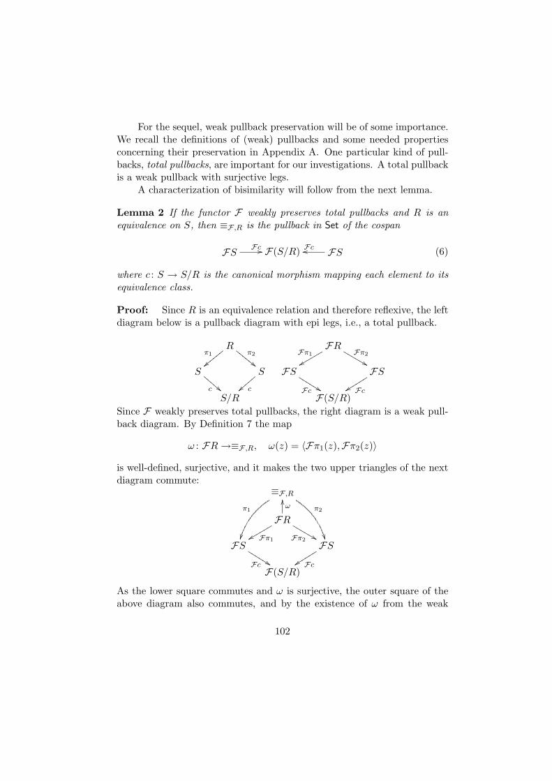
Proof: Since R is an equivalence relation and therefore reflexive, the leftdiagram below is a pullback diagram with epi legs, i.e., a total pullback.

Rπ1

||yyyy

yy π2

""EEE

EEE

S

c !!CCC

CCS

c

S/R

FRFπ1

xxrrrrrr Fπ2

&&LLLLLL

FS

Fc %%KKKKKK FS

Fcyyssssss

F(S/R)

Since F weakly preserves total pullbacks, the right diagram is a weak pull-back diagram. By Definition 7 the map

ω : FR→≡F ,R, ω(z) = 〈Fπ1(z),Fπ2(z)〉

is well-defined, surjective, and it makes the two upper triangles of the nextdiagram commute:

≡F ,R

π1

π2

FR

ωOO

Fπ1xxrrrrrr

Fπ2 &&LLLLLL

FS

Fc %%KKKKKK FS

Fcyyssssss

F(S/R)

As the lower square commutes and ω is surjective, the outer square of theabove diagram also commutes, and by the existence of ω from the weak

102

pullback FR to ≡F ,R, ≡F ,R is a weak pullback as well. However, since ithas projections as legs it is a pullback. ⊓⊔

Suppose that a functor F weakly preserves total pullbacks and assumethat R is an equivalence bisimulation on S, i.e., R is both an equivalencerelation and a bisimulation on S, such that 〈s, t〉 ∈ R. The pullback in Set

of the cospan (6) is the set 〈x, y〉 | Fc(x) = Fc(y) . By Lemma 2 thisset coincides with the lifted relation ≡F ,R. Thus x ≡F ,R y ⇐⇒ Fc(x) =Fc(y). Therefore, we obtain the transfer condition for the particular notionof bisimulation if we succeed in expressing concretely (Fcα)(s) = (Fcα)(t)in terms of the representation of α(s) and α(t).

To illustrate the method, we will use it in showing the well-knowncorrespondence of coalgebraic and concrete bisimulation for LTSs.

Lemma 3 An equivalence relation R on a set S is a coalgebraic bisimula-tion on the LTS 〈S, A, α〉 according to Definition 4 for the functor LA if andonly if it is a concrete bisimulation according to Definition 5.

Proof: It is easy to show that the LTS functor LA preserves weak pullbacks(see e.g. [42]). For X ∈ LA(S), i.e. X ⊆ A × S, we have LA(c)(X) =P〈idA, c〉(X) = 〈idA, c〉(X) = 〈a, c(x)〉 | 〈a, x〉 ∈ X. Using Lemma 1 weget that an equivalence R ⊆ S × S is a coalgebraic bisimulation for an LTS〈S, A, α〉 if and only if

〈s, t〉 ∈ R =⇒ 〈a, c(s′)〉 | 〈a, s′〉 ∈ α(s) = 〈a, c(t′)〉 | 〈a, t′〉 ∈ α(t)

or, equivalently

〈s, t〉 ∈ R =⇒ ( sa−→ s′ =⇒ ∃t′ ∈ S : t

a−→ t′ ∧ 〈s′, t′〉 ∈ R ).

which is the transfer condition from Definition 5. ⊓⊔The most difficult part in establishing the correspondence result for

generative systems is proving the weak pullback preservation for the distri-bution functor.

Proposition 2 The functor D preserves weak pullbacks. ⊓⊔

Appendix B is dedicated to the proof of this proposition. As a con-sequence we get that the functor for generative systems GA preserves weakpullbacks. An application of Lemma 1 and some simple derivations nowsuffice to show the correspondence result.

103

Lemma 4 An equivalence relation R on a set S is a coalgebraic bisimu-lation on the generative system 〈S, A, α〉 according to Definition 4 for thefunctor GA if and only if it is a concrete bisimulation according to Defini-tion 6. ⊓⊔

We end this section with a small discussion on the assumption ofLemma 1. Often we require a functor to weakly preserve pullbacks, sothat it will be “well-behaved”. For example, for bisimilarity being an equiv-alence. It can easily be seen that the milder condition of weakly preservingtotal pullbacks suffices for bisimilarity to be an equivalence. Moreover, wehave relaxed the weak pullback preservation condition since in Section 5 wewill need a bisimilarity characterization of a functor that transforms totalpullbacks to weak pullbacks, but does not preserve weak pullbacks.

3 Weak bisimulation for action-type coalgebras

In this section we present a general definition of weak bisimulation foraction-type systems. Our idea arises as a generalization of the notions ofweak bisimulation for concrete types of systems. In our opinion, a weakbisimulation on a given system is a strong bisimulation on a suitably trans-formed system obtained from the original one.

Weak bisimulation in concrete cases deals with hiding actions. There-fore we focus on weak bisimulation for action-type coalgebras. Recall thatwe have defined action-type coalgebras in Definition 1 as triples 〈S, A, α〉such that 〈S, α : S → FAS〉 is a coalgebra for the functor FA induced by abifunctor F , as in Equation (1).

We proceed with the definition of weak bisimulation for action-typecoalgebras. The definition consists of two phases. First we define the notionof a ∗-extended system, that captures the behavior of the original systemwhen extending from the given set of actions A to A∗, the set of finitewords over A. The ∗-extension should emerge from the original system in afaithful way (which will be made precise below). The second phase considersinvisibility. Given a subset τ ⊆ A of invisible actions, we restrict the ∗-extension to visible behavior only, by defining its weak-τ -extended system.Then a weak bisimulation relation on the original system is obtained as abisimulation relation on the weak-τ -extension.

Definition 8 Let F and G be two bifunctors. Let Φ be a map assigning toevery FA-coalgebra 〈S, A, α〉, a GA∗ system 〈S, A∗, α′〉, on the same set of

104

states S, such that the following conditions are met

(1) Φ is injective, i.e. Φ(〈S, A, α〉) = Φ(〈S, A, β〉)⇒ α = β;

(2) Φ preserves and reflects bisimilarity, i.e. s ∼ t in the system 〈S, A, α〉if and only if s ∼ t in the transformed system Φ(〈S, A, α〉).

Then Φ is called a ∗-translation, notation Φ : F∗→ G. The GA∗-coalgebra

Φ(〈S, A, α〉) is said to be a ∗-extension of the FA-coalgebra 〈S, A, α〉.

From the conditions (1) and (2) in Definition 8 it follows that theoriginal system is “embedded” in its ∗-extension, cf. [10, 11, 43]. The factthat a ∗-translation may lead to systems of a new type, viz. of the bifunctorG, might seem counter intuitive at first sight. However, this extra freedomis exploited in Section 5 when the starting functor itself is not expressiveenough to allow for a ∗-extension.

A way to obtain ∗-translations follows from a previous result. Namely,if λ : FA⇒GA∗ is a natural transformation with injective components andthe functor FA preserves weak pullbacks, then the induced functor (seeEquation (3)) is a ∗-translation [10, 11]. However, we shall see later (cf.Example 1 and the preceding discussion) that ∗-translations emerging fromnatural transformations do not suffice.

Having described how to extend an FA system to its ∗-extension weshow how to hide invisible actions. Fix a set of invisible actions τ ⊆ A.Consider the function hτ : A∗ → (A \ τ)∗ induced by hτ (a) = a if a 6∈ τand hτ (a) = ε for a ∈ τ (where ε denotes the empty word). The functionhτ is deleting all the occurrences of elements of τ in a word of A∗. We putAτ = (A \ τ)∗. By Proposition 1, we get the following.

Corollary 1 The transformation ητ : GA∗⇒GAτ given by ητS = G〈hτ , idS〉

is natural. ⊓⊔

Let Ψτ be the functor from CoalgA∗

G to CoalgAτ

G induced by the naturaltransformation ητ , i.e. Ψτ (〈S, A∗, α′〉) = 〈S, Aτ , α

′′〉 for α′′ = ητS

α′ andΨτf = f for any morphism f : S → T . As mentioned above, the inducedfunctor preserves bisimilarity. The composition of a ∗-translation Φ andthe hiding functor Ψτ is denoted by Ωτ = Ψτ Φ and is called a weak-τ -translation. The resulting system 〈S, Aτ , η

τS

α′〉 is called a weak-τ -extensionof 〈S, A, α〉.

105

The transformation to a weak-τ -extension is presented in the followingscheme.

S

α

Sα′

S

α′′=ητSα′

Φ ///o/o/o/o/o/o/o/o/o/o

Ψτ ///o/o/o/o/o/o/o/o/o/o

FAS GA∗S

FA - coalgebra GA∗ - coalgebra GAτ S

GAτ - coalgebra

A weak-τ -translation, or equivalently, the pair 〈Φ, τ〉, yields a notionof weak bisimulation with respect to Φ and τ .

Definition 9 Let F , G be two bifunctors, Φ : F∗→ G a ∗-translation and

τ ⊆ A. Let 〈S, A, α〉 and 〈T, A, β〉 be two FA systems. A relation R ⊆ S×Tis a weak bisimulation with respect to 〈Φ, τ〉 if and only if it is a bisimulationbetween Ωτ (〈S, A, α〉) and Ωτ (〈T, A, β〉). Two states s ∈ S and t ∈ T areweakly bisimilar with respect to 〈Φ, τ〉, notation s ≈τ t, if they are relatedby some weak bisimulation with respect to 〈Φ, τ〉.

Concrete examples of weak bisimulation will be discussed in Section 4and Section 5. We continue with verifying that weak bisimulations≈τ possesthe intuitively expected properties.

Proposition 3 Let F , G be two bifunctors, Φ : F∗→ G a ∗-translation,

〈S, A, α〉 an FA-coalgebra, τ ⊆ A and let ≈τ denote the weak bisimilarity on〈S, A, α〉 w.r.t. 〈Φ, τ〉. Then the following hold:

(i) ∼ ⊆ ≈τ for any τ ⊆ Ai.e. strong bisimilarity implies weak bisimilarity.

(ii) ∼ = ≈∅

i.e. strong bisimilarity is weak bisimilarity in absence of invisible ac-tions.

(iii) τ1 ⊆ τ2⇒ ≈τ1 ⊆ ≈τ2 for any τ1, τ2 ⊆ A,i.e. the more actions are invisible, the coarser the weak bisimilaritygets.

106

Proof: Let F ,G, Φ, 〈S, A, α〉 and τ be as in the assumptions of theLemma.

(i) Assume s ∼ t in 〈S, A, α〉. Since Φ preserves bisimilarity (Definition 8)we have that s ∼ t in Φ(〈S, A, α〉). Next, since Ψτ preserves bisimi-larity we get s ∼ t in Ψτ Φ(〈S, A, α〉), which by Definition 9 meanss ≈τ t in 〈S, A, α〉.

(ii) From (i) we get ∼ ⊆ ≈∅. For the opposite inclusion, note that h∅ :A∗ → A∗ is the identity map, hence the natural transformation η∅

from Corollary 1 is the identity natural transformation. Therefore theinduced functor Ψ∅ is the identity functor on CoalgA∗

G . Now assumes ≈∅ t in 〈S, A, α〉. This means s ∼ t in Ω∅(〈S, A, α〉), i.e. s ∼ t inΨ∅ Φ(〈S, A, α〉), i.e. s ∼ t in Φ(〈S, A, α〉). Since, by Definition 8,every ∗-translation reflects bisimilarity we get s ∼ t in 〈S, A, α〉.

(iii) Let τ1 ⊆ τ2. Consider the diagram

A∗hτ2 //

hτ1

Aτ2

Aτ1

hτ1,τ2

==

where hτ1,τ2 is the map deleting all occurrences of elements of τ2 in aword of Aτ1 . The diagram commutes since first deleting all occurrencesof elements of τ1 followed by deleting all occurrences of elements of τ2,in a word of A∗ is the same as just deleting all occurrences of elementsof τ2. Let ητ1 , ητ2 , ητ1,τ2 be the natural transformations inducedby hτ1 , hτ2 , hτ1,τ2 , respectively ( see Proposition 1 and Corollary 1).Then the following diagram commutes.

GA∗

ητ2+3

ητ1

GAτ2

GAτ1

ητ1,τ2

8@zzzzzzzz

zzzzzzzz

Let Ψτ1 , Ψτ2 , Ψτ1,τ2 be the functors induced by the natural transfor-mations ητ1 , ητ2 , ητ1,τ2 , respectively. By Equation (3) it holds that

Ψτ2 = Ψτ1,τ2 Ψτ1 (7)

107

and they all preserve bisimilarity. Now assume s ≈τ1 t in 〈S, A, α〉.This means that s ∼ t in the system Ψτ1 Φ(〈S, A, α〉). Then, sinceΨτ1,τ2 preserves bisimilarity we have s ∼ t in the system Ψτ1,τ2 Ψτ1

Φ(〈S, A, α〉) which by equation (7) is the system Ψτ2 Φ(〈S, A, α〉) andwe find s ≈τ2 t in 〈S, A, α〉. ⊓⊔

For further use, we introduce some more notation. For any w ∈ Aτ ,we put Bw = h−1

τ (w) ⊆ A∗. We refer to the sets Bw as blocks. Note thatBw = τ∗a1τ

∗ · · · τ∗akτ∗ for w = a1 . . . ak ∈ Aτ = (A \ τ)∗.

4 Weak bisimulation for LTSs

In this section we show that in the case of LTSs there exists a ∗-translationaccording to the Definition 8, such that weak bisimulation in the concretecase [29] coincides with weak bisimulation induced by this ∗-translation.First we recall the standard definition of concrete weak bisimulation forLTSs.

Definition 10 Let 〈S, A,→〉 be an LTS. Let τ ∈ A be the invisible action.An equivalence relation R ⊆ S × S is a weak bisimulation on 〈S, A, α〉 ifand only if 〈s, t〉 ∈ R implies that

if sa−→ s′, then there exists t′ ∈ S with

tτ−→ ∗

a−→

τ−→ ∗ t′ and 〈s′, t′〉 ∈ R

for all a ∈ A \ τ, and

if sτ−→ s′, then there exists t′ ∈ S with t

τ−→ ∗ t′ and 〈s′, t′〉 ∈ R.

Two states s and t are called weakly bisimilar if and only if they arerelated by some weak bisimulation relation. Notation s ≈ℓ t.

We now present a definition of a ∗-translation that will give rise to anotion of weak bisimulation that coincides with the standard one of Def-inition 10. Recall that L, LA are the functors for LTSs, as introduced inSection 2.

Definition 11 Let Φ assign to every LTS, i.e. any LA-coalgebra 〈S, A, α〉,the LA∗ coalgebra 〈S, A∗, α′〉 where for w = a1 . . . ak ∈ A∗, k > 0,

〈a1 . . . ak, s′〉 ∈ α′(s) ⇐⇒ s

a1−→

a2−→ · · · ak−→ s′

108

and 〈ε, s′〉 ∈ α′(s) ⇐⇒ s = s′. We use the notation sw⇒ s′ for 〈w, s′〉 ∈

α′(s).

Hence, for w = a1 . . . ak, we have sw⇒ s′ if and only if there exist states

s1, . . . , sk−1 such that

sa1−→ s1

a2−→ s2 · · ·ak−1−→ sk−1

ak−→ s′.

Furthermore, note that for a ∈ A, since no hiding applies, it holds that

sa−→ s′ in 〈S, A, α〉 if and only if s

a⇒ s′ in 〈S, A, α′〉 = Φ(〈S, A, α〉)

i.e.,〈a, s′〉 ∈ α(s) ⇐⇒ 〈a, s′〉 ∈ α′(s).

Proposition 4 The assignment Φ from Definition 11 is a ∗-translation.

Proof: We need to prove that Φ is injective and reflects and preservesbisimilarity. Let Φ(〈S, A, α〉) = 〈S, A∗, α′〉, Φ(〈S, A, β〉) = 〈S, A∗, β′〉. As-sume that α′ = β′. Then, for any state s,

〈a, s′〉 ∈ α(s) ⇐⇒ 〈a, s′〉 ∈ α′(s) ⇐⇒ 〈a, s′〉 ∈ β′(s) ⇐⇒ 〈a, s′〉 ∈ β(s).

Hence α(s) = β(s), i.e., α = β.For the reflection of bisimilarity, let s ∼ t in Φ(〈S, A, α〉) = 〈S, A∗, α′〉.

Hence there exists an equivalence bisimulation relation R such that 〈s, t〉 ∈R and (according to Definition 5) for all w ∈ A∗,

if sw⇒ s′ then there exists t′ ∈ S such that t

w⇒ t′ and 〈s′, t′〉 ∈ R.

Assume sa−→ s′ in 〈S, A, α〉. Then s

a⇒ s′ in 〈S, A, α′〉 and therefore

there exists t′ ∈ S with 〈s′, t′〉 ∈ R and ta⇒ t′, i.e., t

a−→ t′. Hence, R is a

bisimulation on 〈S, A, α〉 i.e. s ∼ t in the original system.For the preservation of bisimulation, let s ∼ t in 〈S, A, α〉 and let R be

an equivalence bisimulation relation such that 〈s, t〉 ∈ R. Assume sw⇒ s′,

for some word w ∈ A∗. We show by induction on the length of w thatthere exists t′ with t

w⇒ t′ and 〈s′, t′〉 ∈ R. If w has length 0, then w = ε,

s′ = s and we take t′ = t. Assume w has length k + 1, i.e. w = a · w′ for

a ∈ A, w′ ∈ A∗. Pick s′′ such that sa−→ s′′

w′

⇒ s′. Since 〈s, t〉 ∈ R we can pickt′′ such that t

a−→ t′′ and 〈s′′, t′′〉 ∈ R. By the inductive hypothesis, for w′

we can choose t′ such that t′′w′

⇒ t′ and 〈s′, t′〉 ∈ R. Note that ta−→ t′′

w′

⇒ t′,

109

i.e., tw⇒ t′. Hence R is a bisimulation on 〈S, A∗, α′) and s ∼ t holds in the

∗-extension. ⊓⊔Note that if T is a functor induced by a natural transformation η, in

the context of Equation (3), and if 〈S, A, α〉, 〈S, A, β〉 are two systems suchthat, for some s ∈ S, α(s) = β(s), then, clearly,

α′(s) = ηS(α(s)) = ηS(β(s)) = β′(s) (8)

for 〈S, A, α′〉 = T (〈S, A, α〉), 〈S, A, β′〉 = T (〈S, A, β〉).Having ∗-translations induced by natural transformations is desirable,

since such *-translations are functorial and also obtained by a categori-cal construct. However, the following simple example shows that the ∗-translation Φ from Definition 11 violates (8). Therefore it can not be in-duced by a natural transformation.

Example 1 Let S = s1, s2, s3 and A = a, b, c. Consider the LTSs:

〈S, A, α〉 : s1a−→ s2

b−→ s3 and 〈S, A, β〉 : s1

a−→ s2

c−→ s3.

Obviously α(s1) = β(s1). However, α′(s1) = 〈ε, s1〉, 〈a, s2〉, 〈ab, s3〉while β′(s1) = 〈ε, s1〉, 〈a, s2〉, 〈ac, s3〉.

We next show that the coalgebraic and the concrete definitions coincidein the case of LTS.

Theorem 1 Let 〈S, A, α〉 be an LTS. Let τ ∈ A be the invisible action ands, t ∈ S any two states. Then s ≈τ t with respect to the pair 〈Φ, τ〉 ifand only if s ≈ℓ t.

Proof: Assume s ≈τ t for s, t ∈ S of an LTS 〈S, A, α〉. This means

that s ∼ t in the LTS 〈S, Aτ, ητS

α′〉, i.e., there exists an equivalencebisimulation R on this system with 〈s, t〉 ∈ R.

As usual, α′ is such that 〈S, A∗, α′〉 = Φ(〈S, A, α〉). Here we have

ητS = L(hτ, idS) = P(hτ, idS) and

(ητS

α′)(s) = ητS (α′(s))

= P(hτ, idS)(α′(s))

= 〈hτ(w), s′〉 | 〈w, s′〉 ∈ α′(s)

= 〈u, s′〉 | ∃w ∈ Bu : sw⇒ s′

110

We denote the transition relation of the weak-τ -system 〈S, Aτ, ητS

α′〉by ⇒ τ , i.e., for w ∈ Aτ ,

sw⇒ τ s′ ⇐⇒ 〈w, s′〉 ∈ (η

τS

α′)(s).

The above shows that for a word w = a1 . . . ak ∈ Aτ

sw⇒ τ s′ ⇐⇒ ∃v ∈ Bw = τ∗a1τ

∗ . . . τ∗akτ∗ : s

v⇒ s′.

We will show that the relation R is a weak bisimulation on 〈S, A, α〉 ac-cording to Definition 10. Let s

a−→ s′ (a 6= τ). Then s

a⇒ s′, implying

sa⇒ τ s′. Since R is a bisimulation on the weak-τ -system, there exists

t′ such that ta⇒ τ t′ and 〈s′, t′〉 ∈ R. We only need to note here that

a⇒ τ =

τ−→ ∗

a−→

τ−→ ∗. In case s

τ−→ s′ we have s

τ⇒ s′ implying now

sε⇒ τs

′. Hence, there exists t′ such that tε⇒ τ t

′ and 〈s′, t′〉 ∈ R. Sinceε⇒ τ =

τ−→ ∗, we have proved that R is a weak bisimulation on 〈S, A, α〉

according to Definition 10.For the opposite, let R be a weak bisimulation on 〈S, A, α〉 according

to Definition 10 such that 〈s, t〉 ∈ R. It is easy to show that for any a ∈ A,if s

τ−→ ∗

a−→

τ−→ ∗s′ then there exists t′ such that t

τ−→ ∗

a−→

τ−→ ∗t′

and 〈s′, t′〉 ∈ R. Hence, if sa⇒ τ s′ then there exists t′ with t

a⇒ τ t

′ and〈s′, t′〉 ∈ R. Based on this, a simple inductive argument on k leads to theconclusion that for any word w = a1 . . . ak ∈ Aτ , if s

w⇒ τ s′ then there

exists a t′ such that tw⇒ τ t

′ and 〈s′, t′〉 ∈ R, i.e. R is a bisimulation on theweak-τ -system and hence s ≈τ t. ⊓⊔

5 Weak bisimulation for generative systems

In this section we deal with generative systems and their weak bisimilarity.We first focus on the concrete definition of weak bisimulation by Baier andHermanns [7, 6, 8]. Inspired by it, we provide a functor that suits for adefinition of a ∗-translation for generative systems. This way we obtain acoalgebraic definition of weak bisimulation for this type of systems. Weshow that our definition, although at first sight much stronger, coincideswith the definition of Baier and Hermanns for finite systems. Unlike inthe case of LTSs, for generative systems the ∗-translation needs to leave itsoriginal class of systems, which justifies the generality of the definition.

This section is divided into several parts that lead to the correspon-dence result: First we introduce paths in a generative system and establish

111

some notions and properties of paths. Next we define a measure on theset of paths, where we basically follow the lines of Baier and Hermanns[8, 6]. Furthermore, we present the definition of weak bisimulation by Baierand Hermanns, and we show some properties of weak bisimulation relationsthat will be used later on (without restricting to finite state systems as in[8, 6]). Then we define a translation and prove that it is a ∗-translationproviding us with a notion of weak-τ -bisimulation. The final part of thissection is devoted to the question of correspondence of the notion of weak-τ -bisimulation defined by means of the given ∗-translation and the concretenotion proposed by Baier and Hermanns.

The material presented in this section is to a large extent of technicalnature. For readability, we provide a sketch-of-proof at a number of places.Full proofs can be found in [44].

5.1 Paths and cones in a generative system

Let 〈S, A, P 〉 be a generative system. A finite path π of 〈S, A, P 〉 is analternating sequence 〈s0, a1, s1, a2, . . . , ak, sk〉, where k ∈ N0, si ∈ S, ai ∈ A,and P (si−1, ai, si) > 0, i = 1, . . . , k. We will denote a finite path π =〈s0, a1, s1, a2, . . . , ak, sk〉 more suggestively by

s0a1−→ s1

a2−→ s2 · · · sk−1ak−→ sk .

Moreover, in the situation above, we put

length(π) = k, first(π) = s0, last(π) = sk, trace(π) = a1a2 · · · ak .

The path εs0= (s0) will be understood as the empty path starting at s0.

We will often write just ε for an arbitrary empty path. Similar to the finitecase, an infinite path π of 〈S, A, P 〉 is an infinite sequence 〈s0, a1, s1, a2, . . .〉,where si ∈ S, ai ∈ A and P (si−1, ai, si) > 0, i ∈ N, and will be written as

s0a1−→ s1

a2−→ s2 · · ·

Again we set first(π) = s0. A path π is called complete if it is either infiniteor it is finite with last(π) a terminating state, i.e. P (last(π), , ) = 0.

The sets of all (finite or infinite) paths, of all finite paths and of allcomplete paths will be denoted by Paths, FPaths and CPaths, respectively.Moreover, if s ∈ S, we write

Paths(s) =

π ∈ Paths | first(π) = s

,

FPaths(s) =

π ∈ FPaths | first(π) = s

,

CPaths(s) =

π ∈ CPaths | first(π) = s

.

112

We next define sets of concatenated paths. If Π1, Π2 ⊆ FPaths, wedefine

Π1 ·Π2 =

π1 · π2 | π1 ∈ Π1, π2 ∈ Π2, last(π1) = first(π2)

,

where π1 · π2 ≡ sa1−→ · · ·

ak−→ skak+1−→ · · ·

an−→ sn for π1 ≡ sa1−→ · · ·

ak−→ sk

and π2 ≡ skak+1−→ · · ·

an−→ sn.

The set Paths(s) is partially ordered by the prefix relation. For π, π′ ∈Paths(s) we write π π′ if and only if the path π is a prefix of the pathπ′.

Note that if π ≺ π′ then π is a finite path, and if π1 π and π2 π, then either π1 π2 or π2 π1. The complete paths are exactly themaximal elements in this partial order. For every π ∈ Paths(s), there existsa π′ ∈ CPaths(s) such that π π′.

The following statement will be used at several occasions throughoutthis section.

Lemma 5 For any state s ∈ S, the set FPaths(s) is at most countable.

Proof: Let FPathsn(s) denote the set of finite paths starting from s withlength n. Clearly, FPaths(s) = ∪n∈N FPathsn(s). The statement followsfrom the observation that for any state s and any n ∈ N the set FPathsn(s)is at most countable. This observation can be proven by induction on n asfollows. We have FPaths0(s) = ǫ and

FPathsn+1(s) =⋃

〈a,s′〉:P (s,a,s′)>0

sa−→ s′ · FPathsn(s′)

which is at most countable by the inductive hypothesis and by the factthat P (s, a, s′) > 0 for at most countably many a and s′ (see Lemma 14 inAppendix B). ⊓⊔

Definition 12 For a finite path π ∈ FPaths(s), let π↑ denote the set

π↑ = ξ ∈ CPaths(s) | π ξ

also called the cone of complete paths generated by the finite path π.

Note that always π↑ 6= ∅. Let

Cones(s) =

π↑ | π ∈ FPaths(s)

⊆ P(CPaths(s))

113

denote the set of all cones starting in s. By Lemma 5 this set is at mostcountable. For the study of weak bisimulation for generative systems athorough understanding of the geometry of cones is crucial. To begin with,we have the following elementary property:

Lemma 6 Let π1, π2 ∈ FPaths(s). Then the cones π1↑ and π2↑ are eitherdisjoint or one is a subset of the other. In fact,

π1↑ ∩ π2↑ =

π2↑ if π1 π2

π1↑ if π2 π1

∅ if π1 6 π2 and π2 6 π1

Moreover, we have π1↑ = π2↑ if and only if either

π1 ≡ sa1−→ · · ·

ak−→ sk, π2 ≡ sa1−→ · · ·

ak−→ skak+1−→ sk+1 · · ·

an−→ sn (9)

for n ≥ k ≥ 0, and

P (si−1, ai, si) = 1, i = k + 1, . . . , n (10)

or vice-versa. ⊓⊔

Let Π ⊆ FPaths(s). We say that Π is minimal if for any two π1, π2 ∈ Π,π1 6= π2, we have π1↑ ∩ π2↑ = ∅. Hence in a minimal set of paths Π nopath of Π is a proper prefix of another path of Π. We will express that Π isminimal by writing min(Π). As example note that every singleton set π,π ∈ FPaths(s), is minimal. Also every subset of CPaths(s) is minimal, too.

For Π ⊆ FPaths(s) we denote by Π↑ the set

Π↑ =⋃

π∈Π

π↑ .

Then the fact min(Π) just means that Π↑ is actually the disjoint union ofall π↑, π ∈ Π, i.e.

min(Π) ⇐⇒ Π↑ =⊔

π∈Π

π↑ ,

where, here and in the sequel, the symbol ⊔ denotes disjoint unions. It isan immediate consequence of the definition that,

min(Π), Π′ ⊆ Π =⇒ min(Π′).

114

However, if Π1 and Π2 are minimal, their union need not necessarilybe minimal, even if Π1 ∩Π2 = ∅. We will use the notation

Π =⊎

i∈I

Πi

to express that

Πi ⊆ FPaths(s), i ∈ I, Π =⊔

i∈I

Πi and min(Π) .

Note that if Π =⊎

i∈I Πi, also min(Πi) for all i ∈ I. In particular thisnotation applies to minimal subsets Π written as the union of their one-element subsets:

min(Π) =⇒ Π =⊎

π∈Π

π.

Observe that the following two properties hold, as can be readily checked.

• If Π =⊎

i∈I Πi, then Π↑ =⊔

i∈I Πi↑ =⊔

i∈I,π∈Πiπ↑ .

• We have Π =⊎

i∈I Πi if and only if

– ∀i ∈ I : min(Πi), and

– ∀i, j ∈ I : i 6= j =⇒ Πi ∩Πj = ∅, and

– ∀i, j ∈ I : i 6= j =⇒ ∀πi ∈ Πi,∀πj ∈ Πj : πi 6 πj and πj 6 πi.

Let Π ⊆ FPaths(s). Put Π↓ = π ∈ Π | ∀π′ ∈ Π : π′ 6≺ π.

Lemma 7 For any subset Π ⊆ FPaths(s), it holds that Π↓ ⊆ Π, min(Π↓)and Π↑ =

(

Π↓)

↑. ⊓⊔

5.2 The measure Prob

We proceed with the construction of a probability measure Prob out of thedistribution P of a generative system 〈S, A, P 〉 on a certain σ-algebra onCPaths(s). This method was used in many papers, also in [8, 6], and beforethat in [39], where the setting is slightly different and/or only a part of thestory is given. Here we give complete proofs for our setting. As a standardreference for measure theoretic notions and results we use the monograph[47]. An important measure theoretic result is the extension theorem whichstates that any pre-measure (σ-additive, monotone function with value zero

115

for the empty set) on a semi-ring extends in a unique way to a measureon the σ-field generated by the semi-ring. Slightly different versions of thistheorem apply to different definitions of the notion “semi-ring”. For ourpurposes, the definition of a semi-ring from [47] fits best. Namely, a familyof subsets of a given set S is a semi-ring if it contains the empty set, is closedunder finite intersection and the set difference of any two of its elements isa disjoint union of at most countably many elements of the semi-ring.

Lemma 8 The set Cones(s) ∪ ∅ is a semi-ring.

Proof: Clearly, Cones(s) ∪ ∅ contains the empty set and it is closedunder intersection, by Lemma 6. We need to check that the set-differenceof any two of its elements is a disjoint union of at most countably manyelements of Cones(s)∪ ∅. Let π1↑, π2↑ ∈ Cones(s). We consider π1↑ \ π2↑.Since π1↑ \ π2↑ = π1↑ \ (π1↑ ∩ π2↑), by Lemma 6, the only interesting caseis π1↑ ∩ π2↑ = π2↑ 6= π1↑ which implies π1 ≺ π2. Let

Π = π | π = π′ · last(π′)a−→ s′, π1 π′ ≺ π2, π 6 π2.

Then π1↑ \ π2↑ = Π↑ = ⊔π∈Π π↑. This union is at most countable since theset Π is at most countable by Lemma 5. ⊓⊔

Now we are ready to introduce the desired extension of P to a measure.By Lemma 6, a function Prob : Cones(s) ∪ ∅ → [0, 1] is well-defined byProb(∅) = 0, Prob(ε↑) = Prob(CPaths(s)) = 1 and

Prob(C) = P (s, a, s′) · Prob(C ′), forC = π↑, π = sa−→ s′ · π′, C ′ = π′↑

Lemma 9 The function Prob is a pre-measure4 on the semi-ring Cones(s)∪∅.

Proof: By definition Prob(∅) = 0. Further we need to check mono-tonicity and σ-additivity. To see that Prob is monotonic assume π1↑ ⊆ π2↑.Then, by Lemma 6, we have two possibilities. The first one is π2 ≺ π1 andsince P (s, a, t) ≤ 1 for all s, t ∈ S, a ∈ A, from the definition of Prob we getProb(π1↑) ≤ Prob(π2↑). The second possibility is π1↑ = π2↑, in which caseProb(π1↑) = Prob(π2↑).

For the σ-additivity, assume

π↑ =⊔

i∈I

πi↑ (11)

4In [47] pre-measures are also called measures.

116

for some at most countable index set I. We need to show that Prob(π↑) =∑

i∈I Prob(πi↑).If |I| = 1, then the property is trivially satisfied. Therefore we assume

that |I|> 1. In particular this means that π is not terminating.There exists (via a Lemma of Zorn argument) a partial function depth5

that assigns to some finite paths an ordinal number, satisfying:

1. If ξ ∈ FPaths(s) is such that πi ξ for some i ∈ I, or if ξ terminates,then depth(ξ) = 0.

2. Otherwise, if ξ is a finite path such that all its one step successorsξ′ | ξ ξ′, length(ξ′) = length(ξ) + 1 have assigned depth then alsoξ belongs to the domain of depth and

depth(ξ) = supdepth(ξ′) | ξ ξ′, length(ξ′) = length(ξ) + 1+ 1.(12)

Actually the function depth applied to a finite path ξ captures howdeep in the cone generated by ξ one must go in order to be sure that allextensions of the path under consideration belong to some πi↑ for i ∈ I orterminate. In other words, if depth(ξ) is defined, and if Ξ is the set of pathsthat extend ξ in at least depth(ξ) steps, then any path that extends anypath in Ξ belongs to some of the cones πi↑ for i ∈ I or terminates.

We first show, by reducing to contradiction, that our starting finitepath π has been assigned a value for depth. Assume that π has not beenassigned a value for depth. Let π0 = π. For each i > 0 let πi be a path suchthat length(πi) = length(πi−1) + 1, πi−1 πi and πi has not been assigneda value for depth. Such a chain under the prefix ordering exists since iffor some i all paths that extend πi in one step would had been assigneddepth, then πi would also have been assigned a depth. Consider the infinitecomplete path π∞ such that for all i > 0, πi π∞. By definition π∞ ∈ π↑.By (11), there exists i ∈ I such that π∞ ∈ πi↑, implying that πi π∞ andhence πi = πn for some n ≥ 0. However, then depth(πn) = depth(πi) = 0contradicting that πn has no value for depth assigned.

Let π be any non-terminating path and let πo | o ∈ O be the set ofpaths that extend π in one step, which means that

∀o ∈ O : π ≺ πo, length(πo) = length(π) + 1. (13)

5The function depth has also been defined and used in a proof of a similar propertyby Segala [39].

117

Thenπ↑ =

⊔

o∈O

πo↑ (14)

and

∑

o∈O

Prob(πo↑) =∑

a∈A,s′∈S

Prob(π↑) · P (last(π), a, s′)

= Prob(π↑) ·∑

a∈A,s′∈S

P (last(π), a, s′)

= Prob(π↑) (15)

since π does not end in a terminating state, i.e.∑

a∈A,s∈S P (last(π), a, s) =1.

We finally show, by induction on depth, that if π is a finite path whichhas been assigned a value for depth and if

π↑ =⊔

i∈I′⊆I

πi↑, (16)

for some I ′ ⊆ I, then Prob(π↑) =∑

i∈I′⊆I Prob(πi↑). Assume π is a pathwith depth(π) = 0 satisfying the assumption above. Then either π termi-nates or π↑ = πi↑ for some i ∈ I ′ and therefore |I ′| = 1 and the additivityholds trivially. Now assume depth(π) = α and α is a successor ordinal (bydefinition α can not be a limit ordinal). This implies that π is not terminat-ing. Moreover assume that the property holds for any path of the discussedform with depth smaller than α and let πo | o ∈ O be the set of pathsthat extend π in one step.

By (16) we have that

∀i ∈ I ′ : π πi. (17)

Moreover, from (16) and (14), using Lemma 6 we easily conclude that

∀i ∈ I ′,∃!o ∈ O : πo πi (18)

and∀o ∈ O,∃i ∈ I ′ : πo πi. (19)

LetI ′o = i ∈ I ′ | πo πi.

118

From (16), (18) and (19), we get that I ′o 6= ∅,

I ′ =⊔

o∈O

I ′o and πo↑ =⊔

i∈I′o

πi↑ for o ∈ O. (20)

Then we get

Prob(π↑)(15)=

∑

o∈O

Prob(πo↑)

(I.H.)=

∑

o∈O

∑

i∈I′o

Prob(πi↑)

(20)=

∑

i∈I′

Prob(πi↑).

where the inductive hypothesis is applicable since by (12) and (13),depth(πo) < α for all o ∈ O and I ′o ⊆ I ′ ⊆ I. This completes the proof. ⊓⊔

Corollary 2 The function Prob extends uniquely to a probability measureon the σ-algebra on CPaths(s) generated by Cones(s)∪∅. We will denotethis measure again by Prob. ⊓⊔

Remark 2 Note that, although paths are more or less just alternating se-quences of elements of S and A, whether an alternating sequence of statesand actions is a path depends on the distribution P . Therefore the functionProb itself, but also the σ-algebra where it is defined and in fact already thebase set CPaths(s) depends heavily on P .

The measure Prob induces a function on sets of finite paths, which wewill also denote by Prob. We define Prob : P(FPaths(s))→ [0, 1] by

Prob(Π) = Prob(Π↑).

Note that Π↑ is measurable since it is a countable union of cones. This nota-tion is not in conflict with the already existing notation of the measure Prob.In fact, P(FPaths(s)) ∩ P(CPaths(s)) consists entirely of Prob-measurablesets and on such sets both definitions coincide. To see this, note that ifπ ∈ FPaths(s) ∩ CPaths(s), then π↑ = π. Thus, if Π ⊆ FPaths(s) andΠ ⊆ CPaths(s), we have

Π =⊔

π∈Π

π =⊔

π∈Π

π↑ = Π↑ ,

119

and this union is at most countable.It will always be clear from the context whether we mean the measure

Prob or the just defined function Prob on sets of finite paths. Still, there isa word of caution in order: The function Prob : P(FPaths(s))→ [0, 1] is, ingeneral, not additive. However, looking at the properties of ⊎ introducedabove (on page 115), we find that

Π =⊎

i∈I

Πi =⇒ Prob(Π) =∑

i∈I

Prob(Πi) .

For this reason, we will overload the notation ⊎ and use it also for sets ofcones generated by sets of finite paths, i.e. from now on we will freely write

Π↑ =⊎

i∈I

Πi↑

if and only if it holds that Π =⊎

i∈I Πi for Π, Πi ⊆ FPaths(s).

We obtain that Prob(Π) =∑

π∈Π Prob(π↑) for every minimal set Π.Moreover, by Lemma 7, we always have Prob(Π) = Prob(Π↓).

We next introduce some particular sets of paths. For s ∈ S, S′, S′′ ⊆ Swith S′ ⊆ S′′, and W, W ′ ⊆ A∗ with W ⊆W ′, by

sW→¬W ′

¬S′′

S′

we denote the set of all finite paths that start in s, have a trace in W , endup in S′, without passing a state in S′′ having just performed a trace in theset W ′. Formally,

sW→¬W ′

¬S′′

S′ =

π ∈ FPaths(s) |last(π) ∈ S′, trace(π) ∈W

∀ ξ ≺ π : trace(ξ) 6∈W ′ ∨ last(ξ) 6∈ S′′

.

We write Prob(s, W,¬W, S′,¬S′′) = Prob(sW→¬W ′

¬S′′

S′). Since S′ ⊆ S′′ and

W ⊆ W ′ we always have min(sW→¬W ′

¬S′′

S′). For notational convenience we

will drop redundant arguments whenever possible. Put

sW→¬W ′ S′ = s

W→¬W ′

¬S′

S′,

sW→¬S′′ S′ = s

W→¬W

¬S′′

S′,

sW→ S′ = s

W→¬W

¬S′

S′ ,

(21)

120

and, correspondingly,

Prob(s, W,¬W ′, S′) = Prob(s, W,¬W ′, S′,¬S′),Prob(s, W, S′,¬S′′) = Prob(s, W,¬W, S′,¬S′′),Prob(s, W, S′) = Prob(s, W,¬W, S′,¬S′) .

(22)

Note that

sW→ S′ =

π ∈ FPaths(s) | trace(π) ∈W, last(π) ∈ S′

↓

and hence

Prob(s, W, S′) = Prob(sW→ S′) (23)

= Prob(π ∈ FPaths(s) | trace(π) ∈W, last(π) ∈ S′).

Also, for a ∈ A, t ∈ S, we have

Prob(s, a, t) =

Prob(sa−→ t) = P (s, a, t), if s

a−→ t

Prob(∅) = 0, otherwise(24)

Let S′, S′′, W, W ′ be as above. Suppose F ⊆ S. Then we put

FW→¬W ′

¬S′′

S′ =⊔

s∈F

sW→¬W ′

¬S′′

S′ ⊆ FPaths

In case that for every s ∈ F the value of Prob(s, W,¬W ′, S′,¬S′′) is thesame, we speak of this value as Prob(F, W,¬W ′, S′,¬S′′). Also, in thiscontext, we shall freely apply shorthand as in (21) and (22).

The next technical property concerning sets of concatenated paths will beused at several occasions in the paper. Note that, whenever a concatenationπ1 · π2 is defined, we have Prob(π1 · π2) = Prob(π1) · Prob(π2). Theproof is rather elementary and can be found in [44].

Proposition 5 Let Π1 ⊆ FPaths(s), Π2 ⊆ FPaths and assume that the setof states S is represented as a disjoint union S =

⊔

i∈I Si . Denote Π1,Si=

π1 ∈ Π1 | last(π1) ∈ Si, Π2,t = π2 ∈ Π2 | first(π2) = t. Assume that forevery i ∈ I

Prob(Π2,t′) = Prob(Π2,t′′), t′, t′′ ∈ Si .

Moreover, assume that Π1, Π2 and Π1 · Π2 are minimal. Then, for everychoice of (ti)i∈I ∈

∏

i∈I Si, we have

Prob(Π1 ·Π2) =∑

i∈I

Prob(Π1,Si) · Prob(Π2,ti) .

⊓⊔

121

It is worth to explicitly note the particular case of this propositionwhen |I| = 1.

Corollary 3 Let Π1 ⊆ FPaths(s), Π2 ⊆ FPaths. Let Π2,t = π2 ∈ Π2 |first(π2) = t. Then, if min(Π1), min(Π2) and min(Π1 ·Π2), and if for anyt′, t′′ ∈ first(Π2), Prob(Π2,t′) = Prob(Π2,t′′), we have that

Prob(Π1 ·Π2) = Prob(Π1) · Prob(Π2,t)

for arbitrary t ∈ first(Π2). ⊓⊔

For further reference, we state the following simple property.

Proposition 6 Consider a generative system 〈S, A, P 〉. Let s ∈ S, W ⊆ A∗

and S′ ⊆ S such that it partitions as S′ = ⊔i∈ISi. Then

Prob(s, W, S′) =∑

i∈I

Prob(s, W, Si,¬S′).

Proof: We have sW−→S′ =

⊎

i∈I sW−→ ¬S′Si. ⊓⊔

5.3 The concrete weak bisimulation

In this subsection we recall the original definition of weak bisimulation andbranching bisimulation for generative systems proposed by Baier and Her-manns and we establish some properties of these relations that are essentialfor the correspondence result in Section 5.5 below.

Definition 13 [7, 6, 8] Let 〈S, A, P 〉 be a generative system. Let τ ∈ A bethe invisible action. An equivalence relation R ⊆ S × S is a weak bisim-ulation on 〈S, A, P 〉 if and only if 〈s, t〉 ∈ R implies that for all actionsa ∈ A \ τ and for all equivalence classes C ∈ S/R:

Prob(s, τ∗aτ∗, C) = Prob(t, τ∗aτ∗, C) (25)

and for all C ∈ S/R:

Prob(s, τ∗, C) = Prob(t, τ∗, C). (26)

Two states s and t are weakly bisimilar if and only if they are related bysome weak bisimulation relation. Notation s ≈g t.

122

Note the analogy between the transfer conditions (25), (26) and (4).The definition of branching bisimulation for generative systems is givenbelow.

Definition 14 [7, 6, 8] Let 〈S, A, P 〉 be a generative system. Let τ ∈ Abe the invisible action. An equivalence relation R ⊆ S × S is a branchingbisimulation on 〈S, A, P 〉 if and only if 〈s, t〉 ∈ R implies that for all actionsa ∈ A \ τ and for all equivalence classes C ∈ S/R:

Prob(s, τ∗a, C) = Prob(t, τ∗a, C) (27)

and for all C ∈ S/R:

Prob(s, τ∗, C) = Prob(t, τ∗, C). (28)

Two states s and t are branching bisimilar if and only if they are related bysome branching bisimulation relation. Notation s ≈br

g t.

Baier and Hermanns have shown [6, 8] the following correspondenceresult for finite systems, i.e. systems with finite set of states.

Proposition 7 Any weak bisimulation on a finite generative system is abranching bisimulation and vice versa. Hence, branching bisimilarity andweak bisimilarity coincide on finite systems. ⊓⊔

Also for arbitrary generative systems branching bisimilarity impliesweak bisimilarity, i.e., the proof of this direction of Proposition 7 does notrequire finiteness, as shown below.

Proposition 8 Any branching bisimulation on a generative system is aweak bisimulation as well.

Proof: The property follows since we have sτ∗aτ∗

−→ C =⊎

C′∈S/R sτ∗a−→C ′ ·

C ′ τ∗

−→C given a branching bisimulation R, s ∈ S, a ∈ A and C ∈ S/R. ⊓⊔Whether a coincidence result as in Proposition 7 holds for arbitrary

systems is an open question. The proof for finite systems can not beextended to arbitrary systems - in particular in Lemma 7.5.4 of [6] we cannot obtain regularity for arbitrary matrices. On the other hand, up to now,an example showing the difference between weak and branching bisimilarityfor arbitrary systems is not known to us. Therefore, we distinguish between

123

the two notions.

Let R be a weak or branching bisimulation on 〈S, A, P 〉. Define arelation → on S/R by

C1 → C2 ⇐⇒ Prob(C1, τ∗, C2) = 1

and denote by ↔ the equivalence closure of →, i.e., ↔ = (→ ∪ ←)∗.

A weak or branching bisimulation on 〈S, A, P 〉 is called complete, if

Prob(C1, τ∗, C2) = 1 ⇐⇒ C1 = C2

for all classes C1, C2 ∈ S/R. Hence, if R is a complete weak or branchingbisimulation then for any two different classes C1, C2 ∈ S/R it holds thatProb(C1, τ

∗, C2) < 1.The next proposition is essential for the correspondence result below.

Its proof is long, involved, and includes a detailed study of the → relation.We only give a sketch, details can be found in [44]. A similar property isstated in [8, 6] without a proof.

Proposition 9 Let 〈S, A, P 〉 be a generative system and let s ≈g t or s ≈brg

t. Then there exists a complete weak or a complete branching bisimulationR, respectively, relating s and t.

Proof: (Sketch) The proof follows by a limit argument, using the Lemmaof Zorn, from the following property:

Let R be a weak or branching bisimulation on 〈S, A, P 〉. Let C0 ∈ S/Rbe a fixed class such that U = [C0]↔ 6= C0. Here [C0]↔ denotes the ↔ -equivalence class of C. Define an equivalence R′ on S by

〈s, t〉 ∈ R′ ⇐⇒ 〈s, t〉 ∈ R ∨ s, t ⊆⋃

C∈U

C.

Then R′ is a weak or branching bisimulation, respectively, and R ⊂ R′.Hence, if R is not complete, then a larger weak or branching bisimula-

tion can be derived from it (by joining some classes). ⊓⊔

124

5.4 Weak coalgebraic bisimulation for generative systems

In this subsection we provide a coalgebraic definition of weak bisimulationfor generative systems, according to the approach from Section 3. Forthis we need a ∗-translation that will transform the generative systemswith action set A into systems with action set A∗. Unlike for LTSs, the∗-translation employed will yield coalgebras of a different type.

Let G∗ be the bifunctor defined by

G∗(A, S) = P(A)× P(S)→ [0, 1]

on objects 〈A, S〉 and for morphisms 〈f1, f2〉 : 〈A, S〉 → 〈B, T 〉 by

G∗〈f1, f2〉 = (ν 7→ ν (f−11 × f−1

2 ) | ν : P(A)× P(S)→ [0, 1]).

Consider the Set functor G∗A corresponding to G∗, so that

G∗A(S) = (P(A)× P(S)→ [0, 1])

and for a mapping f : S → T ,

G∗Af(ν) = ν (id−1A × f−1)

for ν : P(A)× P(S)→ [0, 1].We will use the functor G∗A to model the ∗-translation of generative

systems. Therefore we are interested in characterizing equivalence bisimu-lations for this functor. In order to apply the results from Section 2 we needthe following proposition. We dedicate Appendix C to its proof.

Proposition 10 The functor G∗A weakly preserves total pullbacks, but itdoes not preserve weak pullbacks. ⊓⊔

Let R be an equivalence relation on a set S. A subset M ⊆ S is anR-saturated set if for all s ∈M the whole equivalence class of s is containedin M . We denote by Sat(R) the set of all R-saturated sets, Sat(R) ⊆ P(S).Actually, M is a saturated set if and only if M = ∪i∈ICi for Ci ∈ S/R.Hence there is a one-to-one correspondence between the R-saturated setsand the elements of P(S/R).

The next lemma contains a transfer condition for equivalence bisimu-lations for systems of type G∗A. Its proof follows the approach discussed inSection 2 (see Lemma 2 and Lemma 3).

125

Lemma 10 An equivalence relation R on a set S is a bisimulation on theG∗A system 〈S, A, α〉 if and only if

〈s, t〉 ∈ R =⇒ ∀A′ ⊆ A,∀M ∈ Sat(R) : α(s)(A′, M) = α(t)(A′, M).

Proof: Consider the pullback P of the cospan

G∗ASG∗

Ac// G∗A(S/R) G∗AS

G∗

Acoo

where c is the canonical projection of S onto S/R. We have 〈µ, ν〉 ∈ P ifand only if G∗Ac(µ) = G∗Ac(ν), i.e. µ (id−1

A × c−1) = ν (id−1A × c−1). This

is equivalent to

∀A′ ⊆ A,∀M ⊆ S/R : µ(A′, c−1(M)) = ν(A′, c−1(M))

and, since c−1 : P(S/R) → Sat(R) is a bijection, we get an equivalentcondition

∀A′ ⊆ A,∀M ∈ Sat(R) : µ(A′, M) = ν(A′, M).

Now, using Lemma 2, and Proposition 10, we obtain the stated characteri-zation. ⊓⊔

We proceed by presenting a suitable ∗-translation for generative sys-tems. The translation will yield a system of type G∗A∗ . Recall that generativesystems are coalgebras of the functor GA = D(A× Id) + 1.

Definition 15 Let Φg assign to every generative system 〈S, A, P 〉, i.e. anyGA-coalgebra 〈S, A, α〉, the G∗A∗-coalgebra 〈S, A∗, α′〉, where for W ⊆ A∗ andS′ ⊆ S, α′(s)(W, S′) = Prob(s, W, S′).

In order to show that the translation defined above is indeed a ∗-translation we need the property below. Its proof is straightforward andcan be found in [44].

Lemma 11 Let 〈S, A, α〉, i.e. 〈S, A, P 〉, be a GA system, R a bisimulationequivalence on 〈S, A, α〉 and 〈s, t〉 ∈ R. For k ∈ N, Ci ∈ S/R and ai ∈ A,

i ∈ 1, . . . , k, let sa1−→C1 · · ·

ak−→Ck denote the set of paths

sa1−→C1 · · ·

ak−→Ck = sa1−→ s1 · · ·

ak−→ sk | si ∈ Ci, i = 1, . . . , k.

Then sa1−→C1 · · ·

ak−→Ck is minimal and

Prob(sa1−→C1 · · ·

ak−→Ck) = Prob(ta1−→C1 · · ·

ak−→Ck) (29)

⊓⊔

126

We can now show that the defined map is a ∗-translation.

Proposition 11 The assignment Φg from Definition 15 is a ∗-translation.

Proof: We need to check that Φg is injective and preserves and re-flects bisimilarity. For injectivity, assume Φg(〈S, A, α〉) = Φg(〈S, A, β〉) =〈S, A∗, α′〉. Then, by the definition of Prob, cf. (24), we get that for anys, t ∈ S and any a ∈ A, α(s)(〈a, t〉) = P (s, a, t) = Prob(s, a, t) =α′(s)(a, t) = β(s)(〈a, t〉).

Reflection of bisimilarity is direct from Lemma 10: Assume s ∼ t inΦg(〈S, A, α〉) = 〈S, A∗, α′〉 and assume that R is an equivalence bisimulationon 〈S, A∗, α′〉 such that 〈s, t〉 ∈ R. By Lemma 10, we get that for W ⊆ A∗

and for M ∈ Sat(R),

α′(s)(W, M) = α′(t)(W, M). (30)

In particular, for all a ∈ A and all C ∈ S/R, we have

α′(s)(a, C) = α′(t)(a, C). (31)

By the definition of α′ and Prob we have

α′(s)(a, C) = Prob(s, a, C) =∑

s′∈C

P (s, a, s′) =∑

s′∈C

α(s)(〈a, s′〉)

and therefore, for all a ∈ A and all C ∈ S/R,

∑

s′∈C

α(s)(〈a, s′〉) =∑

s′∈C

α(t)(〈a, s′〉) (32)

which means that R is a bisimulation equivalence on the generative system〈S, A, α〉, i.e. s ∼ t in the original system.

The proof of preservation of bisimilarity uses Lemma 11. Let s ∼ tin the generative system 〈S, A, α〉. Then there exists an equivalence bisim-ulation R with 〈s, t〉 ∈ R. The relation R induces an equivalence Rs onFPaths(s) defined by

〈sa1−→ s1 · · ·

ak−→ sk , sa′

1−→ s′1 · · ·a′

k′−→ s′k′〉 ∈ Rs

if and only if k = k′, ai = a′i and 〈si, s′i〉 ∈ R for i = 1, . . . , k. The classes of

Rs are exactly the sets sa1−→C1 · · ·

ak−→Ck for Ci ∈ S/R and ai ∈ A.

127

Assume M ∈ Sat(R) and W ⊆ A∗. We show that the set sW−→M is

saturated with respect to Rs. Namely, let π ≡ sa1−→ s1 · · ·

ak−→ sk ∈ sW−→M

and let π′ ≡ sa1−→ s′1 · · ·

ak−→ s′k be a path such that 〈π, π′〉 ∈ Rs. Thentrace(π) = trace(π′), first(π) = first(π′) and 〈last(π), last(π′)〉 ∈ R. SinceM is saturated, last(π′) ∈ M for last(π) ∈ M . Furthermore, π′ does nothave a proper prefix with trace in W and last in M , since this would imply

that π has such a prefix, contradicting π ∈ sW−→M . Hence, π′ ∈ s

W−→M .

Therefore, the set sW−→M is a disjoint union of some Rs classes and,

since sW→M is minimal, we can write

sW→M =

⊎

i∈I

sai1→ Ci1 · · ·

aiki→ Ciki,

and it follows that Prob(s, W, M) =∑

i∈I Prob(sai1−→Ci1 · · ·

aik−→Cik).

Similarly, tW→ M is a disjoint union of some Rt classes, for Rt being an

equivalence on FPaths(t), defined as Rs with t instead of s. Using that Ris a bisimulation and 〈s, t〉 ∈ R, it is not difficult to see that actually

tW→M =

⊎

i∈I

tai1→ Ci1 · · ·

aiki→ Ciki.

By Lemma 11, we get that Prob(s, W, M) = Prob(t, W, M), i.e.α′(s)(W, M) = α′(t)(W, M) proving that R is a bisimulation on 〈S, A∗, α′〉and s ∼ t in the ∗-extension 〈S, A∗, α′〉. ⊓⊔

The ∗-translation Φg is also not induced by a natural transformation,as the systems of Example 1 in Section 4 show, interpreting each transitionas probabilistic with probability 1.

Remark 3 The ∗-translation Φg together with a subset τ ⊆ A determines aweak-τ -bisimulation. For a generative system 〈S, A, α〉, the weak-τ -systemis

Ψτ Φg(〈S, A, α〉) = Ψτ (〈S, A∗, α′〉) = 〈S, Aτ , α′′〉

where α′′(s) : P(Aτ )× P(S)→ [0, 1] is given by

α′′(s) = ητS(α′(s)) = G∗〈hτ , idS〉(α

′(s)) = α′(s) (h−1τ × id

−1S ).

Hence for X ⊆ Aτ and S′ ⊆ S,

α′′(s)(X, S′) = α′(s)(h−1τ (X), S′) = α′(s)(

⋃

w∈X

Bw, S′) = Prob(s,⋃

w∈X

Bw, S′),

128

where, Bw is the block Bw = τ∗a1τ∗ . . . τ∗akτ

∗ = h−1τ (w), for a word

w = a1 . . . ak ∈ Aτ .Therefore, from Lemma 10 we get that an equivalence relation R is a

weak-τ -bisimulation w.r.t. 〈Φg, τ〉 on the generative system 〈S, A, α〉 if andonly if 〈s, t〉 ∈ R implies that for any collection (Bi)i∈I of blocks writing Bi

as a shorthand for Bwifor some word wi ∈ A∗, and any collection (Cj)j∈J

of classes Cj ∈ S/R,

Prob(s,⋃

i∈I

Bi,⋃

j∈J

Cj) = Prob(t,⋃

i∈I

Bi,⋃

j∈J

Cj). (33)

Sets of the form ∪i∈IBi will be called saturated blocks.

5.5 Correspondence results

We are now able to state and prove the correspondence results for generativesystems. The first statement is obvious from the definitions.

Theorem 2 Let 〈S, A, α〉 be a generative system. Let τ ∈ A be the invisibleaction and s, t ∈ S any two states. Then s ≈τ t according to Definition 9with respect to the pair 〈Φg, τ〉 implies s ≈g t according to Definition 13.

Proof: The statement holds trivially, having in mind Definition 13 andRemark 3, equation (33), since τ∗ as well as τ∗aτ∗, for any a ∈ A \ τ isa saturated block and also each R-equivalence class is an R saturated set.Hence ≈τ is at least as strong as ≈g, ≈τ⊆≈g. ⊓⊔

In the opposite direction we have that coalgebraic weak bisimilarity isimplied by branching bisimilarity.

Theorem 3 Let 〈S, A, α〉 be a generative system. Let τ ∈ A be the invisibleaction and s, t ∈ S any two states. Then s ≈br

g t according to Definition 14implies s ≈τ t according to Definition 9 with respect to the pair 〈Φg, τ〉.

Proof: (Sketch) The proof of this theorem is rather technical, long, anddivided into several steps. Here we discuss its outline. Details can be foundin [44].

Let 〈S, A, P 〉 be a generative system, and s, t ∈ S. Forease of presentation we write Holds[s, t, W, S′] for the statementProb(s, W, S′) = Prob(t, W, S′), where W ⊆ A∗ and S′ ⊆ S. We

129

also write Holds[s, t, W, S′,¬S′′] for the statement Prob(s, W, S′,¬S′′) =Prob(t, W, S′,¬S′′) if needed.

Now assume s ≈brg t for two states s and t. This means that there exists

a branching bisimulation R, according to Definition 14, with 〈s, t〉 ∈ R.Hence, R is an equivalence relation such that for all visible actions a andall equivalence classes C ∈ S/R we have Holds[s, t, τ∗a, C]. AdditionallyHolds[s, t, τ∗, C]. By Proposition 9, we can assume that R is complete (thisis essential for the proof).

We want to show that the transfer condition (33) of Remark 3 holds,and hence R is a coalgebraic weak bisimulation witnessing that s ≈τ t.Therefore, we need to show that for any R-saturated set M = ∪jCj andany union of blocks W = ∪iBi it holds that

Holds[s, t, W, M ].

We establish successively:

1. Holds[s, t, B, C] where B is any block, B = τ∗a1τ∗ . . . τ∗akτ

∗ and Cany class.

2. Holds[s, t, B, Ci,¬M ] for any block B, any saturated set M , andCi ⊆M .

3. Holds[s, t, B, M ] for any block B and any saturated set M .

4. Holds[s, t, W, M ] for any saturated block (i.e. union of blocks) W andany saturated set M .

In each item, the main idea is to represent the set to be measured in termsof the sets for which the statement has already been proved. For example,for the simplest step 1., we observe that for any B′ = τ∗a1τ

∗ . . . τ∗ak wehave

sB′

−→C =⊎

C′∈S/R

sB−→C ′ · C ′ τ∗ak+1

−→ C

and furthers

B−→C =

⊎

C′∈S/R

sB′

−→C ′ · C ′ τ∗

−→C.

130

Step 2. is most involved, but interesting in itself (cf. [44]). Step 3. is adirect consequence of Proposition 6. Showing 4. completes the proof. ⊓⊔

By Theorem 2, Theorem 3, and Proposition 7 we obtain the followingcorollary which gives us the correspondence result for finite systems.

Corollary 4 For finite generative systems, coalgebraic weak bisimilarity≈τ according to Definition 9, with respect to the pair 〈Φg, τ〉, coincideswith concrete weak bisimilarity ≈g according to Definition 13. ⊓⊔

6 Concluding remarks

In this paper, we have proposed a coalgebraic definition of weak bisimulationfor action-type systems. For its justification we have considered the case offamiliar labelled transition systems and of generative probabilistic systems,and we have compared our notion to the concrete definitions. In particular,we have obtained that the coalgebraic definition of weak bisimulation (for asuitably chosen ∗-extension) for LTSs coincides with the standard definitionof weak bisimulation.

For generative probabilistic systems, the situation is more complex.Most of the work and technical difficulties of this paper are related to thecorrespondence results for generative probabilistic systems. As the stan-dard notion of concrete weak bisimulation we have adopted from a numberof choices the one proposed by Baier and Hermanns. However, their in-vestigations and results are limited to finite systems. As our set-up doesnot restrict to the finite case, the coalgebraic framework exploited in thepresent paper extends the concrete definition and provides a coalgebraic def-inition of weak bisimulation for generative systems also covering the infinitecase. Moreover, the correspondence results of our Section 5 also positionthe definition of Baier and Hermanns as a natural one as it is canonicallyinduced from the underlying generative transition systems, once capturedcoalgebraically.

Baier and Hermanns also propose a notion of branching bisimulation.They prove their concrete notions of weak and branching bisimulation tocoincide for finite generative systems. For the coalgebraic definition of weakbisimulation for finite and infinite generative systems the situation is asfollows:

concrete branching ⊆ coalgebraic weak ⊆ concrete weak.

131

As mentioned before, in case of finite systems, we have

concrete branching = concrete weak.

So, in the finite case, that was considered for the concrete notions, allthree notions –concrete branching, coalgebraic weak, and concrete weakbisimulation– coincide. The precise situation of strict inclusion and/orequality for the general case remains to be unraveled, although it seemsthat the coincidence of concrete branching and concrete weak bisimulationwill carry over to a wide class of well-behaved infinite systems.

Various issues remain untackled by the present approach to the weakbisimulation problem for coalgebras. In particular, the main issue here isthat one has to come up with a suitable definition of a ∗-translation oneself,in order to obtain a weak bisimulation for a class of coalgebras of a giventype. Ideally, a coalgebraic construction would automatically induce the ∗-translation. A method for systematically obtaining ∗-translations is a topicfor further research.

Also, other examples that fit in our framework are to be studied. Forinstance, while programs, modeled by automata with outputs for the functorId + O with O being the set of outputs, allow for a coalgebraic definitionof weak bisimulation along the lines described above quite naturally. Theresulting definition coincides with the definition described in [37]. Namely,there the action set is a singleton A = 1 using that Id + O ∼= 1× Id + O.

Acknowledgements

We are indebted to Holger Hermanns for his careful reading and useful com-ments on earlier drafts. We are also grateful for the detailed and constructivefeedback received in the reviewing process of the paper.

References

[1] P. Aczel and N. Mendler. A final coalgebra theorem. In D.H. Pitt,D.E. Rydeheard, P. Dybjer, A.M. Pitts, and A. Poigne, editors, Proc.CTCS’89, pages 357–365. LNCS 389, 1989.

[2] A. Aldini. Probabilistic information flow in a process algebra. In K.G.Larsen and M. Nielsen, editors, Proc. CONCUR’01, pages 152–168.LNCS 2154, 2001.

132

[3] S. Andova, J.C.M. Baeten, and T.A.C. Willemse. A complete axiom-atization of branching bisimulation for probabilistic systems with anapplication in protocol verification. In C. Baier and H. Hermanns,editors, Proc. CONCUR’06, pages 327–342. LNCS 4137, 2006.

[4] S. Andova and T.A.C. Willemse. Equivalences for silent transi-tions in probabilistic systems. In Proc. EXPRESS’04, pages 53–66.ENTCS 128(2), 2005.

[5] S. Andova and T.A.C. Willemse. Branching bisimulation for proba-bilistic systems: characteristics and decidability. Theoretical ComputerScience, 356:325–355, 2006.

[6] C. Baier. On Algorithmic Verification Methods for Probabilistic Sys-tems. Habilitationsschrift, FMI, Universitat Mannheim, 1998.

[7] C. Baier and H. Hermanns. Weak bisimulation for fully probabilis-tic processes. In O. Grumberg, editor, Proc. CAV’97, pages 119–130.LNCS 1254, 1997.

[8] C. Baier and H. Hermanns. Weak bisimulation for fully probabilisticprocesses. Technical Report TR–CTIT–12, Twente University, 1999.

[9] C. Baier, J.-P. Katoen, H. Hermanns, and V. Wolf. Comparativebranching-time semantics for Markov chains. Information and Compu-tation, 200:149–214, 2005.

[10] F. Bartels, A. Sokolova, and E. de Vink. A hierarchy of proba-bilistic system types. In H. Peter Gumm, editor, Proc. CMCS’03.ENTCS 82(1), 2003.

[11] F. Bartels, A. Sokolova, and E. de Vink. A hierarchy of probabilisticsystem types. Theoretical Computer Science, 327:3–22, 2004.

[12] F. Borceux. Handbook of Categorial Algebra, volume 1. CambridgeUniversity Press, 1994.

[13] J. Desharnais, V. Gupta, R. Jagadeesan, and P. Panangaden. Themetric analogue of weak bisimulation for probabilistic processes. InG. Plotkin, editor, Proc. LICS’02, pages 413–422. IEEE, 2002.

133

[14] J. Desharnais, V. Gupta, R. Jagadeesan, and P. Panangaden. Weakbisimulation is sound and complete for PCTL. In L. Brim, P. Jancar,M. Ketınsky, and A. Kuera, editors, Proc. CONCUR’02, pages 355–370. LNCS 2421, 2002.

[15] M. Fiore, G.L. Cattani, and G. Winskel. Weak bisimulation and openmaps. In Proc. LICS’99, Trento, pages 67–76. IEEE, 1999.

[16] R.J. van Glabbeek, S. A. Smolka, B. Steffen, and C. M. N. Tofts.Reactive, generative, and stratified models of probabilistic processes.In Proc. LICS’90, Philadelphia, pages 130–141. IEEE, 1990.

[17] R.J. van Glabbeek, S.A. Smolka, and B. Steffen. Reactive, genera-tive, and stratified models of probabilistic processes. Information andComputation, 121:59–80, 1995.

[18] H. Peter Gumm. Functors for coalgebras. Algebra Universalis, 45:135–147, 2001.

[19] H.P. Gumm. Elements of the general theory of coalgebras. TechnicalReport LUATS’99, Rand Afrikaans University, 1999.

[20] H. A. Hansson. Time and Probability in Formal Design of DistributedSystems. PhD thesis, Uppsala Universitet, 1991.

[21] B.P.F. Jacobs and J.J.M.M. Rutten. A tutorial on (co)algebras and(co)induction. Bulletin of the EATCS, 62:222–259, 1996.

[22] R.M. Keller. Formal verification of parallel programs. Communicationsof the ACM, 19:371–384, 1976.

[23] R. Lanotte, A. Maggiolo-Schettini, and A. Troina. Weak bisimulationfor probabilistic timed automata and applications to security. In Proc.SEFM’03, Brisbane, pages 34–43. IEEE, 2003.

[24] K. G. Larsen and A. Skou. Bisimulation through probabilistic testing.Information and Computation, 94:1–28, 1991.

[25] N. Lopez and M. Nunez. Weak stochastic bisimulation for non-Markovian processes. In Dang Van Hung and M. Wirsing, editors,Proc. ICTAC’05, pages 454–468. LNCS 3722, 2005.

134

[26] S. MacLane. Categories for the working mathematician. Springer-Verlag, 1971.

[27] J. Markovski and N. Trcka. Lumping Markov chains with silent steps.In Proc. QEST’06, Riverside, pages 221–232. IEEE, 2006.

[28] R. Milner. A Calculus of Communicating Systems. LNCS 92, 1980.

[29] R. Milner. Communication and Concurrency. Prentice-Hall, 1989.

[30] R. Milner. Operational and algebraic semantics of concurrent processes.In J. van Leeuwen, editor, Handbook of Theoretical Computer Science,pages 1201–1242. Elsevier and MIT Press, 1990.

[31] L.S. Moss. Coalgebraic logic. Annals of Pure and Applied Logic, 96:277–317, 1999.

[32] A. Philippou, I. Lee, and O. Sokolsky. Weak bisimulation for proba-bilistic systems. In C. Palamidessi, editor, Proc. CONCUR 2000, pages334–349. LNCS 1877, 2000.

[33] G.D. Plotkin. A structural approach to operational semantics. Tech-nical Report DAIMI FN-19, Computer Science Department, AarhusUniversity, 1981.

[34] A. Popescu. Weak bisimilarity coalgebraically. In A. Kurz, M. Lenisa,and A. Tarlecki, editors, Proc. CALCO’09, pages 157–172. LNCS 5728,2009.

[35] J. Rothe. A syntactical approach to weak (bi)-simulation for coalgebras.In L.S. Moss, editor, Proc. CMCS’02. pp. 270–285, ENTCS 65, 2002.

[36] J. Rothe and D. Masulovic. Towards weak bisimulation for coalge-bras. In A. Kurz, editor, Proc. Categorical Methods for Concurrency,Interaction and Mobility. pp. 32–46, ENTCS 68, 2002.

[37] J.J.M.M. Rutten. A note on coinduction and weak bisimilarity forwhile programs. Theoretical Informatics and Applications (RAIRO),33:393–400, 1999.

[38] J.J.M.M. Rutten. Universal coalgebra: A theory of systems. TheoreticalComputer Science, 249:3–80, 2000.

135

[39] R. Segala. Modeling and verification of randomized distributed real-timesystems. PhD thesis, MIT, 1995.

[40] R. Segala and N.A. Lynch. Probabilistic simulations for probabilisticprocesses. In B. Jonsson and J. Parrow, editors, Proc. CONCUR’94,pages 481–496. LNCS 836, 1994.

[41] G. Smith. Probabilistic noninterference through weak probabilisticbisimulation. In Proc. CSFW’03, Pacific Grove, pages 3–13. IEEE,2003.

[42] A. Sokolova. Coalgebraic Analysis of Probabilistic Systems. PhD thesis,TU Eindhoven, 2005.

[43] A. Sokolova and E. de Vink. Probabilistic automata: system types, par-allel composition and comparison. In C. Baier, B.R. Haverkort, H. Her-manns, J.-P. Katoen, and M. Siegle, editors, Validation of StochasticSystems: A Guide to Current Research, pages 1–43. LNCS 2925, 2004.

[44] A. Sokolova, E. de Vink, and H. Woracek. A companion to coalgebraicweak bisimulation for action-type systems. Technical Report CSR 07–12, TU Eindhoven, 2007. 64pp.

[45] M.I.A. Stoelinga. Alea jacta est: verification of probabilistic, real-timeand parametric systems. PhD thesis, Radboud Universiteit Nijmegen,2002.

[46] E. de Vink and J.J.M.M. Rutten. Bisimulation for probabilistic tran-sition systems: a coalgebraic approach. Theoretical Computer Science,221:271–293, 1999.

[47] A.C. Zaanen. An Introduction to the Theory of Integration. North-Holland, 1958.

136

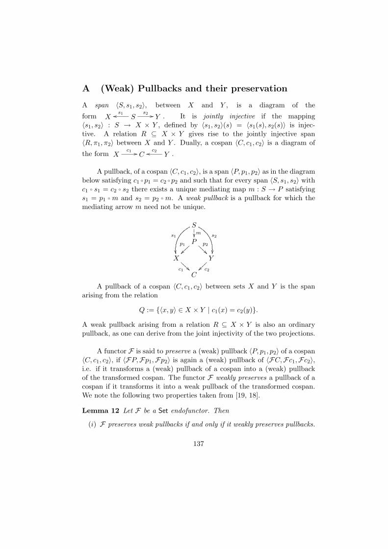
A (Weak) Pullbacks and their preservation

A span 〈S, s1, s2〉, between X and Y , is a diagram of the

form X Ss1oo s2 // Y . It is jointly injective if the mapping

〈s1, s2〉 : S → X × Y , defined by 〈s1, s2〉(s) = 〈s1(s), s2(s)〉 is injec-tive. A relation R ⊆ X × Y gives rise to the jointly injective span〈R, π1, π2〉 between X and Y . Dually, a cospan 〈C, c1, c2〉 is a diagram of

the form Xc1 // C Y

c2oo .

A pullback, of a cospan 〈C, c1, c2〉, is a span 〈P, p1, p2〉 as in the diagrambelow satisfying c1 p1 = c2 p2 and such that for every span 〈S, s1, s2〉 withc1 s1 = c2 s2 there exists a unique mediating map m : S → P satisfyings1 = p1 m and s2 = p2 m. A weak pullback is a pullback for which themediating arrow m need not be unique.

S

s1

s2

m

Pp1

~~

p2

@@@

@

X

c1 AAA

A Y

c2~~~~~~

C

A pullback of a cospan 〈C, c1, c2〉 between sets X and Y is the spanarising from the relation

Q := 〈x, y〉 ∈ X × Y | c1(x) = c2(y).

A weak pullback arising from a relation R ⊆ X × Y is also an ordinarypullback, as one can derive from the joint injectivity of the two projections.

A functor F is said to preserve a (weak) pullback 〈P, p1, p2〉 of a cospan〈C, c1, c2〉, if 〈FP,Fp1,Fp2〉 is again a (weak) pullback of 〈FC,Fc1,Fc2〉,i.e. if it transforms a (weak) pullback of a cospan into a (weak) pullbackof the transformed cospan. The functor F weakly preserves a pullback of acospan if it transforms it into a weak pullback of the transformed cospan.We note the following two properties taken from [19, 18].

Lemma 12 Let F be a Set endofunctor. Then

(i) F preserves weak pullbacks if and only if it weakly preserves pullbacks.

137

(ii) F preserves weak pullbacks if and only if for any cospan 〈C, c1, c2〉we have: Given u and v with Fc1(u) = Fc2(v) then there exists aw ∈ F〈x, y〉 | c1(x) = c2(y) with Fπ1(w) = u and Fπ2(w) = v. ⊓⊔

We end this section by mentioning a special type of pullback. A (weak)pullback 〈P, p1, p2〉 is said to be total if its canonical morphisms, or legs, p1

and p2 are epi. In Set a pullback of a cospan 〈C, c1, c2〉 where c1 : X → Cand c2 : Y → C are surjective, is a total pullback. Moreover, it is easy tosee the following.

Lemma 13 In Set, the pullback of a cospan 〈C, c1 : X → C, c2 : Y → C〉is total if and only if the images of X and Y under c1 and c2, respectively,are equal, i.e. c1(X) = c2(Y ). ⊓⊔

We say that a functor weakly preserves total pullbacks if it transformsany total pullback into a weak pullback. According to Lemma 13, weaklypreserving total pullbacks is the same as weakly preserving pullbacks ofcospans 〈C, c1, c2〉 with c1(X) = c2(Y ). Clearly, if a functor preserves weakpullbacks, then it weakly preserves total pullbacks. We shall see in Ap-pendix C that weak preservation of total pullbacks is a strictly weaker no-tion, i.e., there exists a functor that weakly preserves total pullbacks butdoes not preserve weak pullbacks.

B Weak pullback preservation of the distributionfunctor

Here we establish the weak pullback preservation of GA, the functor defininggenerative probabilistic systems. Actually, we show weak pullback preser-vation of the probability distribution functor D. For the probability distri-bution functor with finite support weak pullback preservation was provenby De Vink and Rutten [46], using the graph-theoretic min cut - max flowtheorem, and by Moss [31], using an elementary matrix fill-in property. Fol-lowing Moss [31] we show that the needed matrix fill-in property can beused and holds for arbitrary, infinite, matrices as well.

We start with a simple auxiliary property, that is also needed for theproof of Lemma 5 (Section 5.1). This property also justifies the name “dis-crete” probability distributions.

138

Lemma 14 Let f : S → R≥0 be a function with the property∑

s∈S f(s) <∞. Then the support set of this function, supp(f) = s ∈ S | f(s) > 0 isat most countable.

Proof: Let s ∈ supp(f). Then f(s)>0 and therefore there exists a naturalnumber n such that f(s)>1/n. So we have, supp(f) ⊆ ∪n∈N suppn(µ) wheresuppn(µ) = s ∈ supp(µ) | f(s)>1/n. Now, since

∑

s∈supp(f) f(s) = r<∞,the set suppn(f) has less than n/r elements, i.e., it is finite , for all n ∈ N.Therefore the set supp(f) is at most countable, being a countable union offinite sets. ⊓⊔

Next we present the matrix fill-in property for infinite matrices.

Lemma 15 Let I and J be arbitrary sets. For any two sets xi | i ∈ Iand yj | j ∈ J of non-negative real numbers such that

∑

i∈I

xi =∑

j∈J

yj <∞,

there exist non-negative real numbers zi,j | i ∈ I, j ∈ J such that

∑

j∈J

zi,j = xi and∑

i∈I

zi,j = yj

for all i ∈ I, j ∈ J .

The proof is rather technical, though interesting, and can be foundin [44, Lemma B.2, Lemma B.3]. Let us discuss the idea, also used in [31]for finite matrices, on a finite example. Let two finite sequences x and y begiven by x1 = 2, x2 = 1, x3 = 3 and y1 = 1, y2 = 3, y3 = 0, y4 = 2. Since

x1 + x2 + x3 = y1 + y2 + y3 + y4

the statement claims that there exists a matrix Z, in this case of order 3×4,such that xi is the sum of the i-th row and yj the sum of the j-th column.The matrix

Z =

1 1 0 00 1 0 00 1 0 2

satisfies that property. We have constructed it in the following way. Forz1,1 we take the minimum minx1, y1, hence z1,1 = y1 = 1. Since the first

139

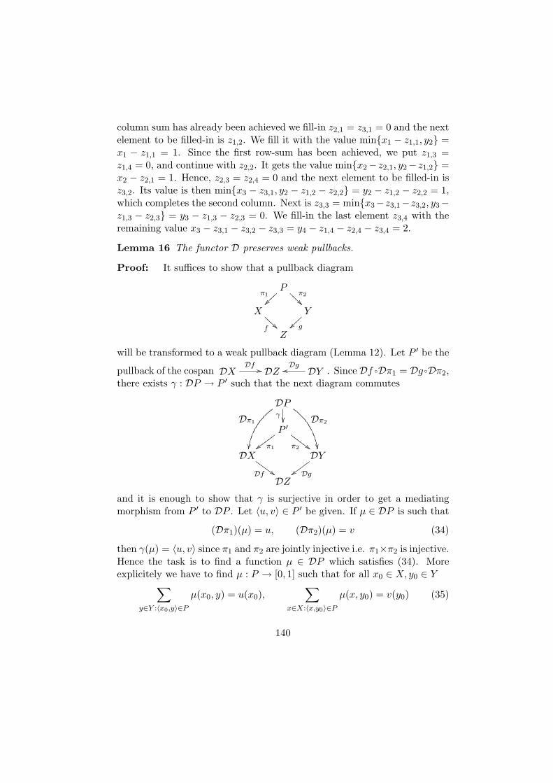
column sum has already been achieved we fill-in z2,1 = z3,1 = 0 and the nextelement to be filled-in is z1,2. We fill it with the value minx1 − z1,1, y2 =x1 − z1,1 = 1. Since the first row-sum has been achieved, we put z1,3 =z1,4 = 0, and continue with z2,2. It gets the value minx2− z2,1, y2− z1,2 =x2 − z2,1 = 1. Hence, z2,3 = z2,4 = 0 and the next element to be filled-in isz3,2. Its value is then minx3 − z3,1, y2 − z1,2 − z2,2 = y2 − z1,2 − z2,2 = 1,which completes the second column. Next is z3,3 = minx3−z3,1−z3,2, y3−z1,3 − z2,3 = y3 − z1,3 − z2,3 = 0. We fill-in the last element z3,4 with theremaining value x3 − z3,1 − z3,2 − z3,3 = y4 − z1,4 − z2,4 − z3,4 = 2.

Lemma 16 The functor D preserves weak pullbacks.

Proof: It suffices to show that a pullback diagram

Pπ1

~~

π2

@@@

@

X

f AAA

A Y

g~~~~~~

Z

will be transformed to a weak pullback diagram (Lemma 12). Let P ′ be the

pullback of the cospan DXDf // DZ DY

Dgoo . Since Df Dπ1 = DgDπ2,there exists γ : DP → P ′ such that the next diagram commutes

DP

Dπ1

Dπ2

γ

P ′

π1wwwww

w

π2 ##GGG

GGG

DX

Df ##HHHHH DY

Dgwwwww

DZ

and it is enough to show that γ is surjective in order to get a mediatingmorphism from P ′ to DP . Let 〈u, v〉 ∈ P ′ be given. If µ ∈ DP is such that

(Dπ1)(µ) = u, (Dπ2)(µ) = v (34)

then γ(µ) = 〈u, v〉 since π1 and π2 are jointly injective i.e. π1×π2 is injective.Hence the task is to find a function µ ∈ DP which satisfies (34). Moreexplicitely we have to find µ : P → [0, 1] such that for all x0 ∈ X, y0 ∈ Y

∑

y∈Y :〈x0,y〉∈P

µ(x0, y) = u(x0),∑

x∈X:〈x,y0〉∈P

µ(x, y0) = v(y0) (35)

140

For if µ : P → [0, 1] satisfies (35), then µ ∈ DP and (34) holds.The set P can be written as the union

P =⋃

z∈Z

f−1(z)× g−1(z)

of disjoint rectangles, in fact rectangles with non-overlapping edges. There-fore, the existence of a map µ which satisfies condition (35) is equiv-alent to the condition that for all z ∈ Z there exists a function µz :f−1(z) × g−1(z) → [0, 1] such that for all x0 ∈ f−1(z), and ally0 ∈ g−1(z),

∑

y∈g−1(z)

µz(x0, y) = u(x0),∑

x∈f−1(z)

µz(x, y0) = v(y0). (36)

Since 〈u, v〉 ∈ P ′, we have

∑

x∈f−1(z)

u(x) = (Df)(u)(z) = (Dg)(v)(z) =∑

y∈g−1(z)

v(y). (37)

Thus we may apply the matrix fill-in property, Lemma 15. ⊓⊔

C Weak pullback preservation of the functor G∗A

In this part we investigate the weak pullback preservation of the functorG∗A. We establish that the functor preserves total weak pullbacks, but doesnot preserve weak pullbacks, i.e. we give a proof of Proposition 10.

Lemma 17 The functor G∗A weakly preserves total pullbacks.

Proof: Let 〈P, π1, π2〉 be a total pullback in Set of the cospan

Xf // Z Y

goo , i.e. P = 〈x, y〉 | f(x) = g(y) and π1, π2 surjec-tive. Then the outer square of the diagram below commutes. More-over, there exists a mediating morphism γ : G∗AP → P ′ from the candi-date pullback 〈G∗AP,G∗Aπ1,G

∗Aπ2〉 to the pullback 〈P ′, p1, p2〉 of the cospan

G∗AXG∗

Af // G∗AZ G∗AYG∗

Agoo .

141

G∗AP

G∗

Aπ1

G∗

Aπ2

γ

P ′

p1zzuuuuu

u

p2 $$III

III

G∗AX

G∗

Af $$HHHHH

G∗AY

G∗

Agvvvvv

G∗AZ

It is enough to prove that γ is surjective (Lemma 12(ii)). So, we showthat for every 〈u, v〉 ∈ P ′ there exists w ∈ G∗AP with G∗Aπ1(w) = u andG∗Aπ2(w) = v which is equivalent to w(id−1

A ×π−11 ) = u and w(id−1

A ×π−12 ) =

v. Fix 〈u, v〉 ∈ P ′. We have

〈u, v〉 ∈ P ′ =⇒ ∀A′ ⊆ A,∀Z ′ ⊆ Z : u(A′, f−1(Z ′)) = v(A′, g−1(Z ′)). (38)

Let X ′ ⊆ X, Y ′ ⊆ Y and assume π−11 (X ′) = π−1

2 (Y ′). Then

(i) f−1(f(X ′)) = X ′:Clearly X ′ ⊆ f−1(f(X ′)). Let x ∈ f−1(f(X ′)) such that f(x) =f(x′) for some x′ ∈ X ′. Since π1 is surjective, there exists y ∈ Ywith 〈x, y〉 ∈ P i.e. f(x) = g(y), and hence also f(x′) = g(y), i.e.〈x′, y〉 ∈ P . Thus 〈x′, y〉 ∈ π−1

1 (X ′) = π−12 (Y ′) implying y ∈ Y ′.

Hence 〈x, y〉 ∈ π−12 (Y ′) = π−1

1 (X ′) i.e. x ∈ X ′.

(ii) g−1(g(Y ′)) = Y ′: similar as (i).

(iii) f(X ′) = g(Y ′):Let z ∈ f(X ′), i.e. z = f(x′) for x′ ∈ X ′. Since π1 is surjective thereexists y ∈ Y with 〈x′, y〉 ∈ P , i.e. f(x′) = g(y). Now, 〈x′, y〉 ∈π−1

1 (X ′) = π−12 (Y ′) and therefore y ∈ Y ′, i.e. z = f(x′) = g(y) ∈

g(Y ′). We have shown f(X ′) ⊆ g(Y ′). Similarly, g(Y ′) ⊆ f(X ′).

Hence, if π−11 (X ′) = π−1

2 (Y ′) for X ′ ⊆ X, Y ′ ⊆ Y we get, for anyA′ ⊆ A,

u(A′, X ′)(i)= u(A′, f−1(f(X ′)))

(38)= v(A′, g−1(f(X ′)))

(iii)=

v(A′, g−1(g(Y ′)))(ii)= v(A′, Y ′).

142

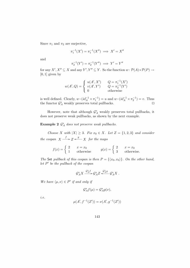
Since π1 and π2 are surjective,

π−11 (X ′) = π−1

1 (X ′′) =⇒ X ′ = X ′′

andπ−1

2 (Y ′) = π−12 (Y ′′) =⇒ Y ′ = Y ′′

for any X ′, X ′′ ⊆ X and any Y ′, Y ′′ ⊆ Y . So the function w : P(A)×P(P )→[0, 1] given by

w(A′, Q) =

u(A′, X ′) Q = π−11 (X ′)

v(A′, Y ′) Q = π−12 (Y ′)

0 otherwise

is well defined. Clearly, w (id−1A ×π−1

1 ) = u and w (id−1A ×π−1

2 ) = v. Thusthe functor G∗A weakly preserves total pullbacks. ⊓⊔

However, note that although G∗A weakly preserves total pullbacks, itdoes not preserve weak pullbacks, as shown by the next example.

Example 2 G∗A does not preserve weak pullbacks.

Choose X with |X| ≥ 3. Fix x0 ∈ X. Let Z = 1, 2, 3 and consider

the cospan Xf // Z X

goo for the maps

f(x) =

2 x = x0

1 otherwiseg(x) =

2 x = x0

3 otherwise.

The Set pullback of this cospan is then P = 〈x0, x0〉. On the other hand,let P ′ be the pullback of the cospan

G∗AXG∗

Af// G∗AZ G∗AX

G∗

Agoo .

We have 〈µ, ν〉 ∈ P ′ if and only if

G∗Af(µ) = G∗Ag(ν),

i.e.µ(A′, f−1(Z ′)) = ν(A′, g−1(Z ′))

143

for all A′ ⊆ A, Z ′ ⊆ Z. Therefore, every pair 〈µ, ν〉 ∈ G∗AX ×G∗AX with theproperty

µ(A′, ∅) = µ(A′, x0) = µ(A′, X \ x0) = µ(A′, X) =

= ν(A′, ∅) = ν(A′, x0) = ν(A′, X \ x0) = ν(A′, X)

belongs to P ′, since ∅, x0, X \ x0 and X are the only subsets of X thatare inverse images of subsets of Z under f and g.

Now we consider G∗AP = P(A) × P(P ) → [0, 1]. If µ ∈ G∗AX is suchthat µ = (G∗Aπ1)(χ) for some χ ∈ G∗AP , then µ = χ (id−1

A × π−11 ). Hence,

for A′ ⊆ A, X ′ ⊆ X we have

µ(A′, X ′) =

χ(A′, ∅) x0 6∈ X ′

χ(A′, 〈x0, x0〉) x0 ∈ X ′.

Choose x1 ∈ X, x1 6= x0. Since |X| ≥ 3 we have x0, x1 6∈ ∅, x0, X \x0, X. Define ξ : P(A)× P(X)→ [0, 1] by

ξ(A′, X ′) =

1 X ′ = x0, x10 otherwise.

Then ξ ∈ G∗A(X) and the pair 〈ξ, ξ〉 belongs to P ′, since for every A′ ⊆ A,

ξ(A′, ∅) = ξ(A′, x0) = ξ(A′, X \ x0) = ξ(A′, X) = 0.

However, ξ can not be written as (G∗Aπ1)(χ) for any χ ∈ G∗AP , since

ξ(A′, x0, x1) 6= ξ(A′, x0),

while, as noted above,

(G∗Aπ1)(χ)(A′, x0, x1) = χ(A′, 〈x0, x0〉) = (G∗Aπ1)(χ)(A′, x0).

Hence, for the pair 〈ξ, ξ〉 ∈ P ′ there does not exist an element χ ∈ G∗APsuch that G∗Aπ1(χ) = ξ and G∗Aπ2(χ) = ξ, which by Lemma 12 shows thatG∗A does not preserve weak pullbacks.

144