Front. Comput. Sci., 2013, 7(3): 359–369

DOI 10.1007/s11704-013-2110-x

Co-metric: a metric learning algorithm for data withmultiple views

Qiang QIAN1, Songcan CHEN 2

1 Department of Computer Science and Engineering, Nanjing University of Aeronautics and Astronautics,

Nanjing 210016, China

2 State Key Laboratory for Novel Software Technology, Nanjing University, Nanjing 210093, China

c© Higher Education Press and Springer-Verlag Berlin Heidelberg 2013

Abstract We address the problem of metric learning for

multi-view data. Many metric learning algorithms have been

proposed, most of them focus just on single view circum-

stances, and only a few deal with multi-view data. In this

paper, motivated by the co-training framework, we propose

an algorithm-independent framework, named co-metric, to

learn Mahalanobis metrics in multi-view settings. In its im-

plementation, an off-the-shelf single-view metric learning al-

gorithm is used to learn metrics in individual views of a few

labeled examples. Then the most confidently-labeled exam-

ples chosen from the unlabeled set are used to guide the met-

ric learning in the next loop. This procedure is repeated until

some stop criteria are met. The framework can accommodate

most existing metric learning algorithms whether types-of-

side-information or example-labels are used. In addition it

can naturally deal with semi-supervised circumstances under

more than two views. Our comparative experiments demon-

strate its competiveness and effectiveness.

Keywords multi-view learning, metric learning, algorithm-

independent framework

1 Introduction

The performance of many machine learning algorithms de-

pend on suitable metrics. Thus in the past decade metric

Received March 26, 2012; accepted July 31, 2012

E-mail: s.chen@nuaa.edu.cn

learning has been extensively studied and many excellent al-

gorithms have been developed [1–3]. However, almost all

of them focus on the single view circumstances. In the real

world, data with natural multiple feature representations is

frequently encountered. For example, web pages can be

represented by both their page contents and the hyperlinks

pointing to them. Video signals naturally consist of acous-

tic and visual signals. In this paper, a new semi-supervised

algorithm-independent metric learning framework for multi-

view settings is developed.

Multi-view metric learning methods belong to two cat-

egories (see Fig. 1): one is learning distance metrics for

each data view by means of carefully exploring multi-view

information [4]. Usually, a method tries to propagate the use-

ful information in one view to guide the learning in another.

The other method is learning distance metrics across different

(a)

(b)

Exchange info between views

d1 (x1

i, x1j ) d2

(x2i, x2

j )

d (x1i, x2

j )

Fig. 1 Two types of multi-view metric. The first measures the distance be-tween examples from within the same views (a), while the second measuresthe distance between examples from two different views (b)

360 Front. Comput. Sci., 2013, 7(3): 359–369

views [5]. Our framework belongs to the first category; for

the remainder of this paper, unless otherwise specified, multi

view learning methods refer to learning distance metrics for

each data view. As far as we know, only the work of Zheng

et al. belongs to this category [4]. However their algorithm

only deals with two-view data and can not utilize unlabeled

examples.

Our framework, called co-metric, is a co-training style

multi-view metric learning framework: given a small initial

labeled and an unlabeled set under multi-view circumstances,

learning multi-view metrics for each view. Co-training is

a successful semi-supervised multi-view classification algo-

rithm proposed by Blum et al. [6]. Its underlying idea is

allowing classifiers learned in different views to teach each

other to boost the classification performance for each view.

We apply this idea to a multi-view metric learning scenario

and propose our co-metric framework: co-metric first learns

one Mahalanobis metric for each view from an existing base

single-view metric learner, then generates some confident su-

pervised information based on the learned metric and adds

it to the current labeled set. The procedure is looped un-

til some stop criteria are met. Our framework is algorithm-

independent, in other words, the framework is built on ex-

isting single-view metric learning algorithms. Thus the di-

rect merit of the framework is its flexibility in utilizing ex-

isting single-view metric learning algorithms as well as their

improved counterparts under different circumstances and its

ease of programming implementation.

Our co-metric algorithm can be treated as a counterpart

of the co-training algorithm in which metric learning is re-

placed by classifier learning. However, there are still some

differences.

First, unlike in the co-training algorithm, co-metric gen-

erates confident supervised information based on the learned

metric through a k nearest neighbor (kNN) classifier. Some

work has been devoted to how to estimate the probabilistic la-

bel of a kNN classifier, however this work is complicated and

focuses on precisely estimating the probabilistic label of the

whole example set [7–9]. Yet co-metric only needs to pick

out some most confidently-labeled examples. Here we devise

a very simple but effective method to pick by choosing those

examples with lots of nearest neighbors sharing the same la-

bels (set the k parameter to a large number, for example 35,

and pick those with the majority of nearest neighbors shar-

ing the same label). Despite its simplicity, this method works

well in our experiments.

Second, classifier learned in co-training algorithm only

takes label supervision, while existing metric learning algo-

rithms may take many types of side information besides la-

bel supervision, for example pairwise squared Euclidean dis-

tance constraints, relative distance constraints, and must-link

and cannot-link constraints (detailed in Section 2). Conse-

quently, before conducting metric learning, the labeled exam-

ples should be converted into suitable side information for-

mats in order to be accepted by the metric learner algorithms

if necessary. Later, we will show that almost all types of side

information can be derived from label supervision.

We list the merits of co-metric as follows:

• It is an algorithm-independent framework, and accom-

modates most of the existing metric learning algo-

rithms.

• It can make use of both labeled examples and unlabeled

examples.

• It naturally deals with dataset with more than two

views.

In Section 2, some related work is reviewed. In Section 3,

a detailed description of co-metric algorithm is provided. Ex-

perimental results are presented in Section 4. Finally the con-

clusion is given in Section 5.

2 Related work

Many algorithms critically depend on good metrics. Conse-

quently metric learning, as a systematic way to discover good

metrics from data, has attracted attention the last decade or

so. Xing et al. [10] proposed a model that minimize the dis-

tances of examples in the similar set while keeping the dis-

tances of examples in the dissimilar set greater than one. This

work shows that the learned metric significantly improves the

clustering performance. Goldberger et al. [3] directly opti-

mized nearest neighbor classifier performance and proposed

neighbourhood components analysis (NCA). Shalev-Shwartz

et al. [11] developed an online metric learning algorithm

pseudo-metric online learning algorithm (PLOA) which op-

timizes a large-margin objective. The algorithm successively

projects the parameters into a positive semi-definite cone and

onto the space constrained by the examples. A regret bound

is also provided. Globerson and Roweis [12] construct a con-

vex optimization problem by collapsing the examples in the

same class into a single point while pushing the examples

in the different classes infinitely far away. Weinberger and

Saul [2] propose a large margin nearest neighbor (LMNN)

algorithm which separates the examples in the same classes

Qiang QIAN et al. Co-metric: a metric learning algorithm for data with multiple views 361

from ones in different classes by a large margin. They con-

sider the algorithm as “a logical counterpart of support vec-

tor machines (SVMs) in which kNN classification replaces

linear classification”. The algorithm is a semi-definite pos-

itive programming problem. Later, they presented an effi-

cient solver [13]. Davis et al. [1] relate every Mahalanobis

distance to a multivariate Gaussian distribution and naturally

measure the distance between two Mahalanobis distances us-

ing Kullback-Leibler divergence between their correspond-

ing Gaussian distributions. The information theoretic metric

learning algorithm (ITML) they proposed minimizes the dis-

tance between the learned Mahalanobis distance and a prior

distance metric under some constraints usually used in a met-

ric learning scenario. The objective of ITML is the Log-

Determninant (LogDet) divergence belongs to the Bregman

divergence family and has some nice properties, thus the

ITML algorithm does not require any eigen-decomposition

and semi-definite positive programming.

In recent years, metric learning algorithms under multi-

view circumstances have also gained attention. As we have

described in Section 1, they can be divided into two cate-

gories: i) metric learning for each view, ii) metric learning

across different views. Algorithms in the first category learn

metric cross the views. Zhai et al. learned a cross-view metric

under semi-supervised situation by forcing the global consis-

tency as well as local smoothness [5]. Their algorithm con-

sists of two steps: 1) seeking a globally consistent and lo-

cally smooth latent space shared by two views; 2) learning

the mapping from the input spaces to the latent space via reg-

ularized locally linear regression. Algorithms in the second

category learn metrics within each view. So far as we know,

the work of Zheng et al. is the only work belonging to this

category [4]. The algorithm they propose is based on NCA.

The objective is composed of three parts. The first two parts

are the summation of the NCA objective function on two sep-

arate views and the third part forces the examples in one view

to be close if they are close in the other view. The algorithm is

applied to audio-visual speaker identification and reports per-

formance superior to standard canonical correlation analysis

algorithm.

As described in Section 1, co-metric is motivated by the

classical co-training algorithm. Co-training is an extensively

studied semi-supervised paradigm for boosting learning per-

formance under multi-view circumstances. Zhou et al. have

shown that the key point in the co-training learning process

is to maintain a large disagreement between base learners

[14, 15]. And that such disagreement is also very important

in semi-superivised active learning [16, 17]. Moreover, this

co-training learning philosophy can be effectively applied in

many multi-view algorithm designs. For example, Nigam and

Ghani [18] analyzed the effectiveness of the co-training com-

pare with EM on merged views and proposed co-EM algo-

rithm. Brefeld and Scheffer [19] integrated SVM into co-EM

algorithm by converting the outputs of SVM into a probabilis-

tic form and modify SVM to incorporate probabilistically la-

beled instances and introduced co-EM SVM algorithm. Ku-

mar and Daume [20] proposed a multi-view spectral cluster-

ing algorithm. It follows the co-training scheme and alterna-

tively clusters the samples in one view, and uses the clustering

results to modify the spectral structure in another view.

3 The algorithm framework

3.1 Some notations

First we introduce some notations used in the paper. Fol-

lowing the co-training circumstances, we are given a small

labeled set and an unlabeled set. The example and the la-

bel are denoted by x and y, respectively. We have a multi-

view datasetD = L∪U, where L = {(x1, y1), . . . , (x|L|, y|L|)}and U = {x|L|+1, . . . , x|L|+|U|} are the labeled and unlabeled

sets, respectively. Typically we have abundant unlabeled

data because it is easy to collect, but usually we have only

a few labeled data because labels are hard to gather. Each

example xi is given as a tuple (x1i , . . . , x

Vi ) that corresponds

to V different views. For the ease of notation, we define

Lv = {(xv1, y1), . . . , (xv

|L|, y|L|)} and Uv = {xv|L|+1, . . . , x

v|L|+|U|}.

For each view v, co-metric tries to learn a Mahalanobis dis-

tance defined as dAv(xvi , x

vj) = (xv

i − xvj)

T Av(xvi − xv

j) where Av

is a positive semi-defined matrix.

3.2 Multi-view metric learning

The goal of multi-view metric learning is to learn suitable

distance metrics from each data view from a few labeled ex-

amples as well as some unlabeled ones for multi-view data.

Multi-view data is frequently encountered in real world ap-

plications. For example, web pages can be represented by

their page contents and the hyperlinks pointing to them and

senses can be captured from different viewing angles et al.

The subject was first touched on Yarowsky [21]. Later, a

famous semi-supervised multi-view learning method, called

co-training was introduced (and is still widely used) by Blum

and Mitchell [6]. It works in an iterative manner; in each

round, co-training first trains one classifier on the labeled set

for each separate view. Then it adds a portion of confidently-

362 Front. Comput. Sci., 2013, 7(3): 359–369

labeled unlabeled examples for each classifiers to the labeled

set, and retrains the classifiers for each view. Intuitively the

underlying idea is to use the learned information from one

view to teach the learning in another view. Although co-

training is applied in a semi-supervised learning situation, the

underlying idea is also made use of in the other tasks like un-

supervised clustering [20, 22].

We introduce this idea to a multi-view metric learning sce-

nario, and design a co-training style multi-view metric learn-

ing framework called co-metric. Figure 2 shows the flow

chart of the co-metric algorithm when there are two data

views. Compared with co-training algorithm flow, co-metric

contains an additional convertion step (second step in Fig. 2).

This is because the existing metric learning algorithms take

many different types of side information as supervision be-

sides labels. Thus an additional step converting the label su-

pervision into suitable side information accepted by the base

metric learner is necessary. Also, most types of side informa-

tion can be derived straightforwardly from label information

shown as follows:

Initial labeled sample set

Learn metric on View 1 from existing metric learning algorithm

Generate new confident sample labels based on learned metric

Merge the new confident sample labels into labeled sample set

Learn metric on View 2 from existing metric learning algorithm

Generate new confident sample labels based on learned metric

Convert sample labels into other typesof supervised inf ormation acceptedby base metric learning algorithms

Fig. 2 The flow chart of co-metric algorithm under two data views

• Pairwise squared Euclidean distance constraints

dAv(xvi , x

vj) � lv, if yi = y j, (1)

dAv(xvi , x

vj) � uv, if yi � y j, (2)

where lv and uv are two constant lower and upper thresholds.

• Relative distance constraints

dAv(xvi , x

vj) � dAv(xv

i , xvk), if yi = y j and yi � yk. (3)

•Must-links and Cannot-links

(xvi , x

vj) ∈ Must-link set, if yi = y j, (4)

(xvi , x

vj) ∈ Cannot-link set, if yi � y j. (5)

In a co-training algorithm, how to choose the confidently-

labeled examples given the newly-learned classifiers in each

view is the most critical and tricky part. Much effort has been

devoted to finding methods for choosing the confidently-

labeled examples in a co-training algorithm [23]. Unlike co-

training, co-metric chooses the confidently-labeled examples

in each view based on the learned metrics. Thus the most

straightforward way is to attach the probabilistic labels to un-

labeled examples by a kNN classifier from the learned met-

rics, and choose the most confidently-labeled examples. So

far, much work examines prediction methods for probabilis-

tic labels of kNN classifier [7–9]. Holmes and Adams [8]

proposed Bayesian probabilistic nearest neighbor (PNN) in

which both K and the interaction between neighbors are as-

signed prior distributions; this gives a marginal prediction

with proper probabilities. But empirical study shows that

the performance is of PNN does not improve on kNN [24].

Later, some extensions of PNN were developed to improve

the overall performance [7, 25]. However, the computation

of both PNN and its extension are complicated and depend

on sampling methods like Markov chain Monte Carlo sam-

pling or Gibbs sampling. In this paper, we develop a very

simple method based on the following observations: 1) we

do not need to precisely estimate the probabilistic labels

of all the unlabeled examples, we only need to identify a

few confidently-labeled examples from unlabeled set. It is

a comparatively easy task because errors in estimating low

confidence-labled examples are acceptable; 2) an unlabeled

example can be confidently classified if many of its nearest

neighbors have the same label. Consequently co-metric iden-

tifies the confidently-labeled examples through employing a

simple discrete prediction, defined as follows:

p(x is in class c) =number of nearest neighbors in class c

K,

(6)

when K is large (e.g., K = 35). The unlabeled examples, with

the top largest discrete prediction, are chosen as confidently-

labeled examples. Moreover, a large threshold (for exam-

ple 90%) can also be introduced to make the choice safer.

Note that we only need to identify a few examples, thus such

a strict condition is acceptable. Figure 3 demonstrates this

idea. In this figure, four blue stars are unlabeled examples.

Too identify the confidently-labeled examples, kNN algo-

rithm (K = 35) is applied. In Fig. 3, the k nearest neighbors

of the unlabeled examples are enclosed by circles. The un-

labeled examples in the cyan circles are confidently-labeled

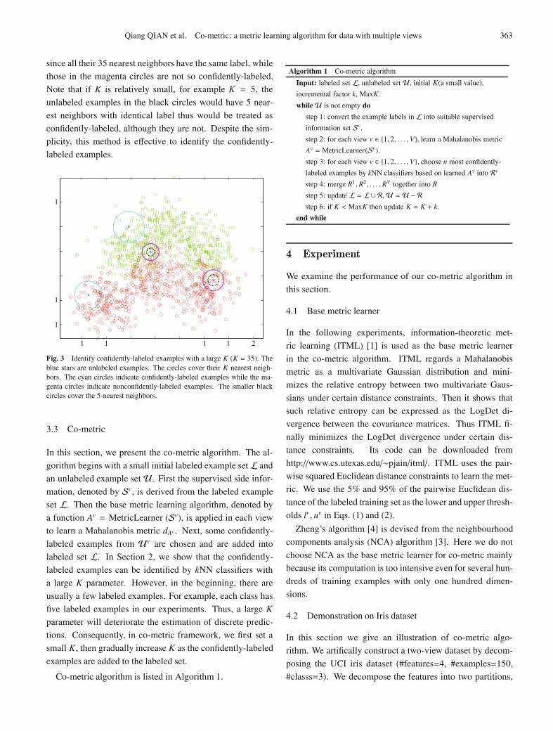
Qiang QIAN et al. Co-metric: a metric learning algorithm for data with multiple views 363

since all their 35 nearest neighbors have the same label, while

those in the magenta circles are not so confidently-labeled.

Note that if K is relatively small, for example K = 5, the

unlabeled examples in the black circles would have 5 near-

est neighbors with identical label thus would be treated as

confidently-labeled, although they are not. Despite the sim-

plicity, this method is effective to identify the confidently-

labeled examples.

Fig. 3 Identify confidently-labeled examples with a large K (K = 35). Theblue stars are unlabeled examples. The circles cover their K nearest neigh-bors. The cyan circles indicate confidently-labeled examples while the ma-genta circles indicate nonconfidently-labeled examples. The smaller blackcircles cover the 5-nearest neighbors.

3.3 Co-metric

In this section, we present the co-metric algorithm. The al-

gorithm begins with a small initial labeled example setL and

an unlabeled example set U. First the supervised side infor-

mation, denoted by Sv, is derived from the labeled example

set L. Then the base metric learning algorithm, denoted by

a function Av = MetricLearner (Sv), is applied in each view

to learn a Mahalanobis metric dAv . Next, some confidently-

labeled examples from Uv are chosen and are added into

labeled set L. In Section 2, we show that the confidently-

labeled examples can be identified by kNN classifiers with

a large K parameter. However, in the beginning, there are

usually a few labeled examples. For example, each class has

five labeled examples in our experiments. Thus, a large K

parameter will deteriorate the estimation of discrete predic-

tions. Consequently, in co-metric framework, we first set a

small K, then gradually increase K as the confidently-labeled

examples are added to the labeled set.

Co-metric algorithm is listed in Algorithm 1.

Algorithm 1 Co-metric algorithm

Input: labeled set L, unlabeled setU, initial K(a small value),

incremental factor k, MaxK.

whileU is not empty do

step 1: convert the example labels in L into suitable supervised

information set Sv.

step 2: for each view v ∈ {1, 2, . . . ,V}, learn a Mahalanobis metric

Av = MetricLearner(Sv).

step 3: for each view v ∈ {1, 2, . . . ,V}, choose n most confidently-

labeled examples by kNN classifiers based on learned Av into Rv

step 4: merge R1,R2, . . . ,RV together into R

step 5: update L = L ∪ R,U = U − Rstep 6: if K < MaxK then update K = K + k.

end while

4 Experiment

We examine the performance of our co-metric algorithm in

this section.

4.1 Base metric learner

In the following experiments, information-theoretic met-

ric learning (ITML) [1] is used as the base metric learner

in the co-metric algorithm. ITML regards a Mahalanobis

metric as a multivariate Gaussian distribution and mini-

mizes the relative entropy between two multivariate Gaus-

sians under certain distance constraints. Then it shows that

such relative entropy can be expressed as the LogDet di-

vergence between the covariance matrices. Thus ITML fi-

nally minimizes the LogDet divergence under certain dis-

tance constraints. Its code can be downloaded from

http://www.cs.utexas.edu/∼pjain/itml/. ITML uses the pair-

wise squared Euclidean distance constraints to learn the met-

ric. We use the 5% and 95% of the pairwise Euclidean dis-

tance of the labeled training set as the lower and upper thresh-

olds lv, uv in Eqs. (1) and (2).

Zheng’s algorithm [4] is devised from the neighbourhood

components analysis (NCA) algorithm [3]. Here we do not

choose NCA as the base metric learner for co-metric mainly

because its computation is too intensive even for several hun-

dreds of training examples with only one hundred dimen-

sions.

4.2 Demonstration on Iris dataset

In this section we give an illustration of co-metric algo-

rithm. We artifically construct a two-view dataset by decom-

posing the UCI iris dataset (#features=4, #examples=150,

#classs=3). We decompose the features into two partitions,

364 Front. Comput. Sci., 2013, 7(3): 359–369

one for each view. Each view has two features, this can be

visualized in two-dimensional space. The examples are ran-

domly split into two even sets, one for training and the other

for testing. three examples per class are randomly chosen

from the training set as the labeled set, and the rest are the

unlabeled set. K is initially set to 3, this is equal to the num-

ber of examples per class in the initial labeled set. The in-

cremental factor k is set to 2. Figure 4 demonstrates the clas-

sification results of the 3NN classifier with the learned Ma-

halanobis metrics at the different iterations in co-metric al-

gorithm as well as the corresponding heatmap of the learned

Mahalanobis metrics. For comparison, Fig. 4 also illustrates

the results on the whole supervised training dataset (including

both labeled set and unlabeled set with labels) on its bottom

row.

• Classification results

Clearly, the classification results on both views gradually

Fig. 4 3NN classification results of co-metric on iris dataset in 13 iterations with ITML as the base metric learner. (Left column: theclassification results on View 1. Middle column: the classification results on View 2. Right column: the heatmaps of learned Mahalanobismetrics. The top 3 rows: results of co-metric. Bottom row: results of full supervised metric learning.)

Qiang QIAN et al. Co-metric: a metric learning algorithm for data with multiple views 365

increases as co-metric makes progress. Compared with the

full supervised results, the final classification areas and the

learned metrics of co-metric are almost the same on both

views. The 3NN classification accuracy increases from

74.6% to 98.7% and from 88.0% to 94.7% on View 1 and

View 2 respectively, which is a considerable boost.

View independence plays an important role in a co-training

style algorithm. Higher view independence is favored and

potentially gives better results [6]. Since co-metric is a co-

training style algorithm, such a statement should also be

right. In Section 5, some experiments are conducted to study

this statement. Here we simply show the view independence

in Table 1. “1” indicates complete dependence and “0” in-

dicates complete independance. We can see that the view

dependence between View 1 and View 2 is very low. That

assures the success of co-metric on this dataset.

Table 1 View correlation on the dataset measured by linear kernel align-ment

Name View 1 View 2

View 1 1.00 0.08

View 2 0.08 1.00

• Our method of choosing confidently-labeled examples

Next, we show the quality of the chosen confidently-

labeled examples by our simple method. Figure 5 shows

the accuracy of the labeled set after the chosen confidently-

labeled examples are added at each iteration. For the first few

iterations, the accuracy stays at 100%, then drops a little, but

remains above 98% for the whole procedure. Consequently,

our simple method works well. Note that when the accuracy

drops at iteration 11, it does not keep dropping but ascends

at the following two iterations. This means that even as the

Fig. 5 The accuracy of the labeled set at each iteration on iris dataset

accuracy becomes lower, our simple method still can possibly

choose the right confidently-labeled examples.

4.3 Performance study of co-metric algorithm

In this section we examine the performance of our co-metric

algorithm. First we introduce the baseline used in our ex-

periments. Then we briefly describe the datasets used in our

experiments and the experimental settings. Finally we show

the experiment results.

4.3.1 Baseline

• Single view (SV) Learn the metric on the labeled

set on each view alone.

• Feature concatenation (FC) Learn the metric on the

concatenated features from each view.

• DCCA [26] Loosely speaking, any linear dimen-

sion reduction algorithm can also be boiled down to a

metric learning procedure, although the so-called met-

ric resulting from any dimension reduction algorithm is

actually a pseudo metric which is not strictly positive

definite and does not always guarantee xi = x j when

d(xi, x j) = 0. Thus discriminative canonical correlation

analysis, as a supervised variant of classical canonical

correlation analysis which can incorporate the label in-

formation, is also introduced as a baseline.

• Zheng’s method (Zheng) [4] A multi-view metric

learning algorithm built on the NCA algorithm. So far

as we know, this is the only multi-view metric learning

method. The λ parameter in this algorithm is chosen

from [10−2, 10−1, 100, 101, 102] and the best results are

reported.

4.3.2 Dataset

• The multiple feature (handwritten) digit dataset

(MFD)1)

MFD dataset is from UCI machine learning repository

[27]. It consists of features of handwritten numerals

(“0”–“9”) extracted from a collection of Dutch utility

maps. Each numeral has 200 examples (for a total of

2 000 examples) with six feature sets (Fac, Fou, Kar,

Pix, Zer, Mor). As declared in Section 1, one of the

prerequisites of co-metric is that each view should sat-

isfy the sufficiency condition. Thus we remove two fea-

ture sets (Zer, Mor) which have large gaps between their

performances (less than 80%) and the top performance

1) http://archive.ics.uci.edu/ml/datasets/Multiple+Features

366 Front. Comput. Sci., 2013, 7(3): 359–369

(above 95%) on the other four views with full super-

vised information.

• Course dataset

This dataset consists of 1 051 web pages collected from

Computer Science department websites at four univer-

sities. Each page is represented by its content and the

text on the links to it, and thus has two views. These

pages have two classes: course and non-course. The

dimensions of this dataset are relatively high (1 840, 3

000 for each view). Learning such large matrices in

Mahalanobis metric it is easy to overfit and computa-

tionally prohibitive. Consequently we reduce the di-

mensions of both views to 100 with the standard latent

semantic analysis method [28].

• 20 newsgroups dataset

We artificially construct a four view two class dataset

from the twenty news categories described in Table

2. For each positive and negative class, we randomly

choose 800 examples from the corresponding news cat-

egories. To avoid overfitting and the intensive compu-

tational burden, the dimensions are also reduced to 100

from 61 189 with latent semantic analysis.

Table 2 The setup of news dataset

View Positive class Negative class

News1 comp.graphics comp.sys.ibm.pc.hardware

News2 rec.motorcycles rec.sport.baseball

News3 sci.crypt sci.med

News4 talk.politics.guns talk.religion.misc

Note that our co-metric can naturally deal with multiple

views larger than two. However, two baselines (DCCA and

Zheng) only deal with two views. Thus, multi-view datasets

are broken down into multiple two-view sub-datasets in the

following experiments.

4.3.3 Experimental settings

The examples are randomly split into two even partitions, one

for training and the other for testing. In the following exper-

iments, we want to test whether co-metric can self-boost its

performance from a small portion of labeled examples with

the help of unlabeled examples. Thus only a small portion of

labeled examples are used in these experiments. Specifically

only five examples per class are randomly chosen from the

training set as the labeled set and the rest are the unlabeled

set. The initial K is set to 5, equal to the number of examples

of each class in the initial labeled set. To keep K odd, the

incremental factor k is set to 2. MaxK is set to 35. The classi-

fication accuracy of the kNN classifier is reported. Note that

the K parameter in the kNN classifier can influence the accu-

racy. To avoid such influence, we run 1NN, 3NN, 5NN, 7NN

and 9NN, and report the highest accuracy. For each experi-

ment, ten trials are run and the mean accuracy and standard

deviation are reported.

4.3.4 Accuracy analysis: two view learning

The experiment results are demonstrated in Table 3. In the

table, the best results are bolded.

Table 3 kNN classification accuracy comparison under two view circum-stance

co-metric SV FC DCCA Zheng

Fac 88.0±1.5 76.1±0.3 81.0±3.2 80.7±3.3 66.8±3.7

Fou 80.0±1.0 72.4±2.2 56.2±2.7 70.2±2.1

Fac 93.0±1.0 76.1±0.3 85.3±3.0 80.7±3.3 66.9±3.4

Kar 93.8±1.6 84.9±2.2 56.4±4.2 82.0±3.7

Fac 93.2±0.6 76.1±0.3 86.4±2.3 80.7±3.3 65.3±3.7

Pix 94.8±0.6 85.7±2.1 78.2±3.9 84.0±2.5

Fou 80.7±1.2 72.4±2.2 88.7±1.9 56.2±2.7 70.0±2.8

Kar 88.0±1.2 84.9±2.2 56.5±4.2 82.0±2.9

Fou 80.9±0.9 72.4±2.2 91.1±1.7 56.7±2.7 69.2±2.7

Pix 89.2±1.0 85.7±2.1 78.2±3.9 83.1±2.7

Kar 94.8±0.6 84.9±2.2 85.6±2.3 56.5±4.2 80.1±3.5

Pix 95.4±0.8 85.7±2.1 78.2±3.9 82.5±2.6

Page 92.1±1.4 79.4±9.7 88.5±2.8 85.5±4.3 87.8±3.7

Link 92.4±0.9 85.8±1.9 80.9±17.9 88.1±2.7

News1 80.6±4.4 59.4±7.3 64.4±7.1 65.4±9.3 63.3±7.7

News2 79.2±2.8 62.6±3.6 62.5±4.9 64.2±4.8

News1 75.7±8.6 59.4±7.3 64.7±6.6 65.3±9.4 63.4±7.7

News3 73.7±10.4 63.4±7.8 66.5±6.4 70.7±8.0

News1 75.8±8.1 59.4±7.3 65.0±8.2 65.3±9.3 63.4±7.8

News4 73.0±8.7 66.4±7.0 73.5±9.3 67.7±8.2

News2 81.2±3.9 62.6±3.6 66.5±6.6 62.5±4.9 64.2±4.6

News3 79.4±3.6 63.4±7.8 66.4±6.4 70.2±8.2

News2 77.6±6.5 62.6±3.6 66.0±6.6 62.5±4.9 63.9±4.2

News4 76.7±6.6 66.4±7.0 73.5±9.3 67.8±8.1

News3 68.9±7.8 63.4±7.8 63.6±7.2 66.4±6.4 71.1±8.1

News4 67.2±8.4 66.4±7.0 73.5±9.3 67.8±8.4

The single view metric learning and concatenated features

metric learning set the baseline of the other algorithms. Con-

catenating features in multiple view into a single one is the

most straightforward method to conduct multi-view learn-

ing although it has some inherent flaws [29]. In our exper-

iment, most of the time feature concatenation only get close

or slightly better results comparing with single view learning.

Our co-metric algorithm gains the best classification accu-

racies, only losses on five out of twenty-six views. Co-metric

manages to outperform the single view metric learning by

ten percent on average and the concatenated view learning

Qiang QIAN et al. Co-metric: a metric learning algorithm for data with multiple views 367

by about six percent. Its ability for exploring multiple view

information and unlabeled information makes it learn better

metrics.

DCCA achieves better performance against single view

and feature concatenation on 20 newsgroup dataset but fails

on both the MFD and Course dataset. One reason for this is

that the maximum reduced dimension is limited by the class

numbers because the rank of the matrix in the DCCA’s ob-

jective is at most equal to the class numbers. Thus, DCCA

may lose some useful information after dimension reduction

due to this defect. While metric learning algorithms (here

ITML) directly learning Mahalanobis distance has no such

limitations. When the dimension of the dataset is not large

(at most about two hundred), learning full Mahalanobis dis-

tance is a better choice. As a result, DCCA cannot overtake

single view metric learning on MFD and Course dataset even

DCCA can explore multiple views information. DCCA also

cannot perform better than co-metric algorithm in most of the

experiments. Because compared with co-metric, DCCA does

not make use of unlabeled examples. When the initial labeled

set is small, DCCA cannot produce a satisfactory classifica-

tion performance.

Next we see how Zheng performs. Zheng has lower ac-

curacy on 12 views during all six experiments on the MFD

dataset, and achieves higher accuracy during seven experi-

ments on Course and 20 newsgroup datasets. It can be seen

that Zheng cannot always boost performance when the la-

beled training set is very small. Compared with DCCA,

Zheng achieves better results on 17 out of 26 total views.

This again verifies that directly learning Mahalanobis dis-

tance can yield better results than rank-limited dimension re-

duction method DCCA. However Zheng fails to yield better

results against our co-metric algorithm. It is reasonable be-

cause Zheng does not explore unlabeled examples.

4.3.5 The Influence of view independence on performance

In this section, we show how the view independence influ-

ences the performance. According to [6], co-training works

better when more independent views are used because learn-

ing on the independent views will bring new independent

labels. Intuitively, this statement should also hold in our

co-metric framework, and in our experiment this is verified.

Although the view independence condition can be relaxed

to relatively loose ε-expanding condition [30], it is relatively

hard to quantify. Thus in this experiment we instead choose

kernel alignment (KA) [31] to measure the view indepen-

dence for its simplicity and interpretability. In terms of KA

measure, perfectly positively-correlated views have the high-

est score 1, perfectly negatively-correlated views have the

lowest score -1 and totally independent views have the score

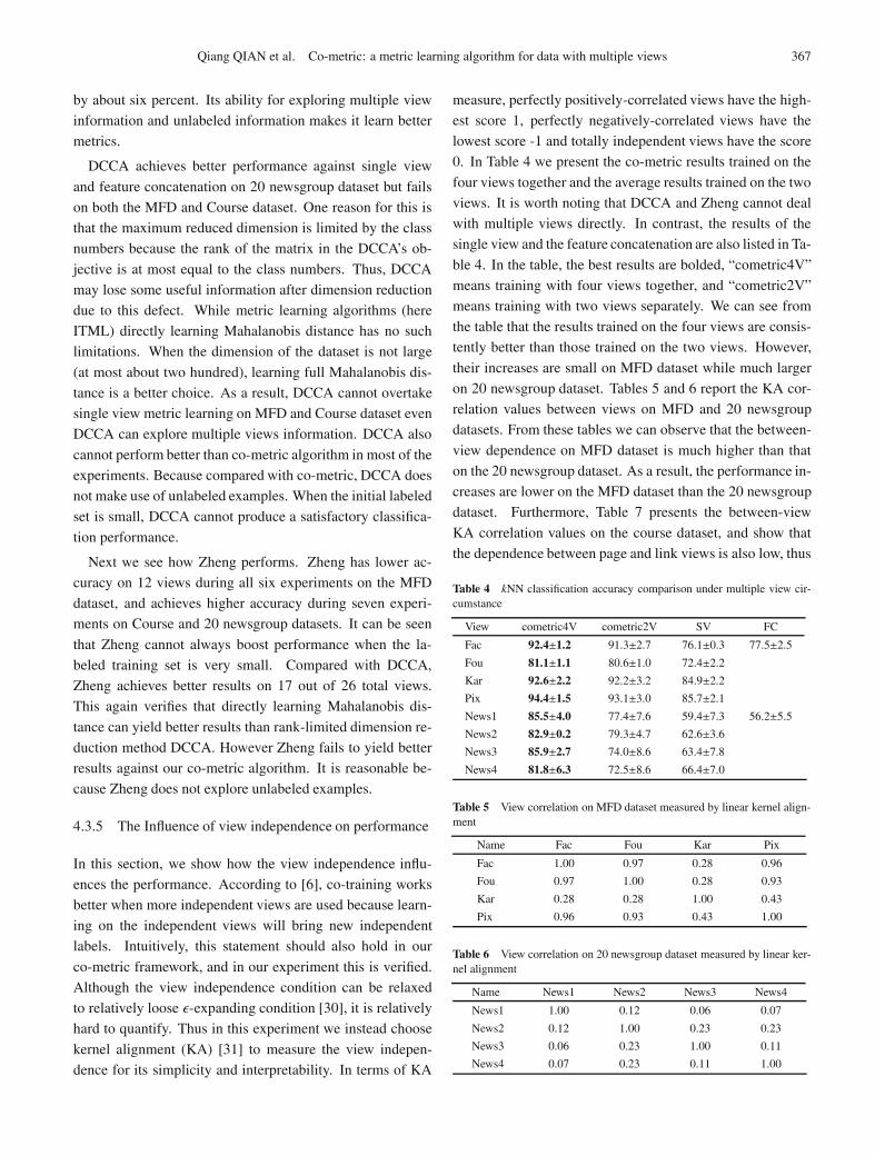
0. In Table 4 we present the co-metric results trained on the

four views together and the average results trained on the two

views. It is worth noting that DCCA and Zheng cannot deal

with multiple views directly. In contrast, the results of the

single view and the feature concatenation are also listed in Ta-

ble 4. In the table, the best results are bolded, “cometric4V”

means training with four views together, and “cometric2V”

means training with two views separately. We can see from

the table that the results trained on the four views are consis-

tently better than those trained on the two views. However,

their increases are small on MFD dataset while much larger

on 20 newsgroup dataset. Tables 5 and 6 report the KA cor-

relation values between views on MFD and 20 newsgroup

datasets. From these tables we can observe that the between-

view dependence on MFD dataset is much higher than that

on the 20 newsgroup dataset. As a result, the performance in-

creases are lower on the MFD dataset than the 20 newsgroup

dataset. Furthermore, Table 7 presents the between-view

KA correlation values on the course dataset, and show that

the dependence between page and link views is also low, thus

Table 4 kNN classification accuracy comparison under multiple view cir-cumstance

View cometric4V cometric2V SV FC

Fac 92.4±1.2 91.3±2.7 76.1±0.3 77.5±2.5

Fou 81.1±1.1 80.6±1.0 72.4±2.2

Kar 92.6±2.2 92.2±3.2 84.9±2.2

Pix 94.4±1.5 93.1±3.0 85.7±2.1

News1 85.5±4.0 77.4±7.6 59.4±7.3 56.2±5.5

News2 82.9±0.2 79.3±4.7 62.6±3.6

News3 85.9±2.7 74.0±8.6 63.4±7.8

News4 81.8±6.3 72.5±8.6 66.4±7.0

Table 5 View correlation on MFD dataset measured by linear kernel align-ment

Name Fac Fou Kar Pix

Fac 1.00 0.97 0.28 0.96

Fou 0.97 1.00 0.28 0.93

Kar 0.28 0.28 1.00 0.43

Pix 0.96 0.93 0.43 1.00

Table 6 View correlation on 20 newsgroup dataset measured by linear ker-nel alignment

Name News1 News2 News3 News4

News1 1.00 0.12 0.06 0.07

News2 0.12 1.00 0.23 0.23

News3 0.06 0.23 1.00 0.11

News4 0.07 0.23 0.11 1.00

368 Front. Comput. Sci., 2013, 7(3): 359–369

Table 7 View correlation on course dataset measured by linear kernelalignment

Name Page Link

Page 1.00 0.23

Link 0.23 1.00

comparing the single view results of Table 3, co-metric also

has likewise better performance.

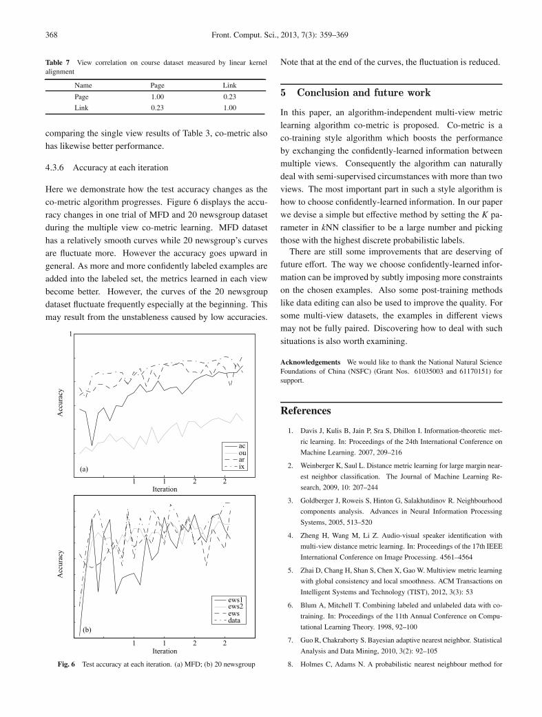
4.3.6 Accuracy at each iteration

Here we demonstrate how the test accuracy changes as the

co-metric algorithm progresses. Figure 6 displays the accu-

racy changes in one trial of MFD and 20 newsgroup dataset

during the multiple view co-metric learning. MFD dataset

has a relatively smooth curves while 20 newsgroup’s curves

are fluctuate more. However the accuracy goes upward in

general. As more and more confidently labeled examples are

added into the labeled set, the metrics learned in each view

become better. However, the curves of the 20 newsgroup

dataset fluctuate frequently especially at the beginning. This

may result from the unstableness caused by low accuracies.

Fig. 6 Test accuracy at each iteration. (a) MFD; (b) 20 newsgroup

Note that at the end of the curves, the fluctuation is reduced.

5 Conclusion and future work

In this paper, an algorithm-independent multi-view metric

learning algorithm co-metric is proposed. Co-metric is a

co-training style algorithm which boosts the performance

by exchanging the confidently-learned information between

multiple views. Consequently the algorithm can naturally

deal with semi-supervised circumstances with more than two

views. The most important part in such a style algorithm is

how to choose confidently-learned information. In our paper

we devise a simple but effective method by setting the K pa-

rameter in kNN classifier to be a large number and picking

those with the highest discrete probabilistic labels.There are still some improvements that are deserving of

future effort. The way we choose confidently-learned infor-

mation can be improved by subtly imposing more constraints

on the chosen examples. Also some post-training methods

like data editing can also be used to improve the quality. For

some multi-view datasets, the examples in different views

may not be fully paired. Discovering how to deal with such

situations is also worth examining.

Acknowledgements We would like to thank the National Natural ScienceFoundations of China (NSFC) (Grant Nos. 61035003 and 61170151) forsupport.

References

1. Davis J, Kulis B, Jain P, Sra S, Dhillon I. Information-theoretic met-

ric learning. In: Proceedings of the 24th International Conference on

Machine Learning. 2007, 209–216

2. Weinberger K, Saul L. Distance metric learning for large margin near-

est neighbor classification. The Journal of Machine Learning Re-

search, 2009, 10: 207–244

3. Goldberger J, Roweis S, Hinton G, Salakhutdinov R. Neighbourhood

components analysis. Advances in Neural Information Processing

Systems, 2005, 513–520

4. Zheng H, Wang M, Li Z. Audio-visual speaker identification with

multi-view distance metric learning. In: Proceedings of the 17th IEEE

International Conference on Image Processing. 4561–4564

5. Zhai D, Chang H, Shan S, Chen X, Gao W. Multiview metric learning

with global consistency and local smoothness. ACM Transactions on

Intelligent Systems and Technology (TIST), 2012, 3(3): 53

6. Blum A, Mitchell T. Combining labeled and unlabeled data with co-

training. In: Proceedings of the 11th Annual Conference on Compu-

tational Learning Theory. 1998, 92–100

7. Guo R, Chakraborty S. Bayesian adaptive nearest neighbor. Statistical

Analysis and Data Mining, 2010, 3(2): 92–105

8. Holmes C, Adams N. A probabilistic nearest neighbour method for

Qiang QIAN et al. Co-metric: a metric learning algorithm for data with multiple views 369

statistical pattern recognition. Journal of the Royal Statistical Soci-

ety: Series B (Statistical Methodology), 2002, 64(2): 295–306

9. Tomasev N, Radovanovic M, Mladenic D, Ivanovic M. A proba-

bilistic approach to nearest-neighbor classification: naive hubness

bayesian kNN. In: Proceedings of the 20th ACM International Con-

ference on Information and Knowledge Management. 2011, 2173–

2176

10. Xing E, Ng A, Jordan M, Russell S. Distance metric learning, with

application to clustering with side-information. Advances in Neural

Information Processing Systems. 2002, 505–512

11. Shalev-Shwartz S, Singer Y, Ng A. Online and batch learning of

pseudo-metrics. In: Proceedings of the 21st International Conference

on Machine Learning. 2004, 94–103

12. Globerson A, Roweis S. Metric learning by collapsing classes. Ad-

vances in Neural Information Processing Systems, 2006

13. Weinberger K, Saul L. Fast solvers and efficient implementations for

distance metric learning. In: Proceedings of the 25th International

Conference on Machine Learning. 2008, 1160–1167

14. Zhou Z, Li M. Semi-supervised learning by disagreement. Knowl-

edge and Information Systems, 2010, 24(3): 415–439

15. Zhou Z. Unlabeled data and multiple views. In: Proceedings of the

1st IAPR TC3 Conference on Partially Supervised Learning. 2011,

1–7

16. Zhou Z, Chen K, Dai H. Enhancing relevance feedback in image re-

trieval using unlabeled data. ACM Transactions on Information Sys-

tems (TOIS), 2006, 24(2): 219–244

17. Wang W, Zhou Z. Multi-view active learning in the non-realizable

case. arXiv preprint arXiv:1005.5581, 2010

18. Nigam K, Ghani R. Analyzing the effectiveness and applicability of

co-training. In: Proceedings of the 9th International Conference on

Information and Knowledge Management(CIKM2000). 2000

19. Brefeld U, Scheffer T. Co-em support vector learning. In: Proceed-

ings of the 21st International Conference on Machine Learning. 2004,

16–24

20. Kumar A, Daume III H. A co-training approach for multi-view spec-

tral clustering. In: Proceedings of the 28th IEEE International Con-

ference on Machine Learning. 2011

21. Yarowsky D. Unsupervised word sense disambiguation rivaling su-

pervised methods. In: Proceedings of the 33rd Annual Meeting on

Association for Computational Linguistics. 1995, 189–196

22. Bickel S, Scheffer T. Multi-view clustering. In: Proceedings of the

Fourth IEEE International Conference on Data Mining. 2004, 19–26

23. Zhang M, Zhou Z. coTrade: confident co-training with data editing.

IEEE Transactions on Systems, Man, and Cybernetics, Part B: Cyber-

netics, 2011, 41(6): 1612–1626

24. Manocha S, Girolami M. An empirical analysis of the probabilis-

tic k-nearest neighbour classifier. Pattern Recognition Letters, 2007,

28(13): 1818–1824

25. Cucala L, Marin J, Robert C, Titterington D. A Bayesian reassessment

of nearest-neighbor classification. Journal of the American Statistical

Association, 2009, 104(485): 263–273

26. Sun T, Chen S, Yang J, Shi P. A novel method of combined feature

extraction for recognition. In: Proceedings of 8th IEEE International

Conference on the Data Mining. 2008, 1043–1048

27. Frank A, Asuncion A. UCI machine learning repository, 2010.

http://archive.ics.uci.edu/ml

28. Dumais S. Latent semantic analysis. Annual Review of Information

Science and Technology, 2004, 38(1): 188–230

29. Sa V R, Gallagher P, Lewis J, Malave V. Multi-view kernel construc-

tion. Machine Learning, 2010, 79(1): 47–71

30. Balcan M, Blum A, Ke Y. Co-training and expansion: towards bridg-

ing theory and practice. Advances in Neural Information Processing

Systems, 2004

31. Shawe-Taylor N, Kandola A. On kernel target alignment. In: Ad-

vances in Neural Information Processing Systems. 2002

Qiang Qian received his BSc from

Nanjing University of Aeronautics and

Astronautics (NUAA), China. Cur-

rently he is a PhD student at the Depart-

ment of Computer Science and Engi-

neering, NUAA. His research interests

include data mining and pattern recog-

nition.

Songcan Chen received his BSc in

mathematics from Hangzhou Univer-

sity (now merged into Zhejiang Uni-

versity) in 1983. In December 1985,

he completed the MSc in computer ap-

plications at Shanghai Jiaotong Univer-

sity and began working at Nanjing Uni-

versity of Aeronautics and Astronautics

(NUAA) from January 1986 as an assistant lecturer. There he re-

ceived a PhD degree in communication and information systems in

1997. Since 1998, as a full professor, he has been with the Depart-

ment of Computer Science and Engineering at NUAA. His research

interests include pattern recognition, machine learning, and neural

computing. In these fields, he has authored or coauthored over 130

scientific journal papers.