CO isotopologues in the Perseus Molecular Cloud Complex: the X-factor and

regional variations

Jaime E. Pineda

Harvard-Smithsonian Center for Astrophysics, 60 Garden St., MS-10, Cambridge, MA 02138,USA

jpineda@cfa.harvard.edu

Paola Caselli

School of Physics and Astronomy, University of Leeds, LS2 9JT, UK

INAF, Osservatorio Astrofisico di Arcetri, Largo E. Fermi 5, I-50125 Firenze, Italy

p.caselli@leeds.ac.uk

and

Alyssa A. Goodman

Harvard-Smithsonian Center for Astrophysics, 60 Garden St., MS-42, Cambridge, MA 02138,USA

agoodman@cfa.harvard.edu

ABSTRACT

The COMPLETE Survey of Star-Forming regions offers an unusually comprehensiveand diverse set of measurements of the distribution and temperature of dust and gas inmolecular clouds, and in this paper we use those data to find new calibrations of the“X-factor” and the 13CO abundance within Perseus. To carry out our analysis, we: 1)apply the NICER (Near-Infrared Color Excess Method Revisited) algorithm to 2MASSdata to measure dust extinction; 2) use dust temperatures derived from re-processedIRAS data; and 3) make use of the 12CO and 13CO (1-0) transition maps gathered byCOMPLETE to measure gas distribution and temperature. Here, we divide Perseusinto six sub-regions, using groupings in a plot of dust temperature as a function ofLSR velocity. The standard X factor, X ≡ N(H2)/W (12CO), is derived both for thewhole Perseus Complex and for each of the six sub-regions with values consistent withprevious estimates. However, the X factor is heavily affected by the saturation of theemission above AV∼4 mag, and variations are found between regions. We derive linearfits to relate W (12CO) and AV using only points below 4 mag of extinction. Thislinear fit yields a better estimation of the AV than the X factor. We derive linear

– 2 –

relations of W (13CO), N(13CO) and W (C18O) with AV . In general, the extinctionthreshold above which 13CO (1-0) and C18O (1-0) are detected is about 1 mag largerthan previous estimates, so that a more efficient shielding is needed for the formationof CO than previously thought. The fractional abundances (w.r.t. H2 molecules) arein agreement with previous works. The (1-0) lines of 12CO and 13CO saturate above4 and 5 mag, respectively, whereas C18O (1-0) never saturates in the whole AV rangeprobed by our study (up to 10 mag). Approximately 60% of the positions with 12CO (1-0) emission have sub-thermally excited lines, and almost all positions have 12CO (1-0)excitation temperatures below the dust temperature. We compare our data with PDRmodels using the Meudon code, finding that 12CO (1-0) and 13CO (1-0) emission canbe explained by these uniform slab models with densities ranging between about 103

and 104 cm−3. In general, local variations in the volume density and non-thermalmotions (linked to different star formation activity) can explain the observations. Higherdensities are needed to reproduce CO data toward active star forming sites, such asNGC 1333, where the larger internal motions driven by the young protostars allow morephotons from the embedded high density cores to escape the cloud. In the most quiescentregion, B5, the 12CO and 13CO emission appears to arise from an almost uniform thinlayer of molecular material at densities around 104 cm−3, and the integrated intensitiesof the two CO isotopologues are the lowest in the whole complex.

Subject headings: dust, extinction — ISM:abundances — ISM:molecules — ISM:individual(Perseus molecular complex)

1. Introduction

Although H2 is the most abundant molecule in the interstellar medium (by about four ordersof magnitude), it cannot be used as a tracer of the physical conditions in a molecular cloud.In fact, being a homonuclear species, H2 does not have an electric dipole moment and even thelowest (electric quadrupole) rotational transitions require temperatures and densities well abovethose found in typical molecular clouds. The next most abundant molecule is 12CO, and since itsdiscovery by Wilson et al. (1970) it has been considered the best tracer of H2 and the total massof molecular clouds (e.g. Combes 1991). Because of its relatively large abundance and excitationproperties, the 12CO (1-0) line is typically optically thick in molecular clouds, so that rarer COisotopomers (in particular 13CO) have also been used to trace the cloud mass in the most opaqueregions. However, previous attempts to derive cloud masses from the thinner isotopomers presenta large scatter (factor of 10), indicating that 13CO line strength is not an entirely straightforwardindicator of gas column. In particular, the following points should be taken into account to deriveless uncertain conversions: 1) preferential photodissociation of 13CO at low optical extinctions, AV ;2) active chemical fractionation in the presence of 13C+ ions, enhancing the relative abundance of13CO in cold gas (Watson 1977); and 3) variations in the 12CO/13CO abundance ratio across the

– 3 –

Galaxy.

The conversion between 12CO (1-0) integrated intensity (W (12CO)) and H2 column density(N(H2)) is usually made using the so-called “X-factor,” defined as

X ≡ N(H2)W (12CO)

. (1)

In order to calibrate this ratio, one needs to measure the column of H2 which is difficult to doreliably.

One method to derive this ratio uses only the 12CO emission and the assumption that molecularclouds are close to virial equilibrium. Solomon et al. (1987) found a tight relation between themolecular cloud virial mass and the 12CO luminosity (MVT = 39(LCO)0.81). This relation enabledthem to derive a ratio of 3.0× 1020 cm−2 K−1 km−1 s for the median mass of the sample (105 M�).In this case, the main source of uncertainty is the assumption of virial equilibrium for the molecularclouds.

Another method uses the generation of gamma rays by the collision of cosmic rays with Hand H2. The H2 abundance is calculated using (assumed optically thin) 21-cm observations of H Iand gamma ray observations in concert. Bloemen et al. (1986) using COS-B data derived a valueof (2.8 ± 0.4) × 1020 cm−2 K−1 km−1 s for the X factor, while Strong & Mattox (1996) derived(1.9 ± 0.2) × 1020 cm−2 K−1 km−1 s using the EGRET data. Uncertainties in gamma-ray-derivedestimates of the X-factor stem from coarse resolution (0.5◦ and 0.2◦ for COS-B and EGRET,respectively) and from the assumption that there are no point sources of gamma rays.

An alternative method to derive the column density of H2 makes use of the IRAS 100 µm datato estimate the total column density of dust, which can then be used, assuming a constant dust-to-gas ratio (=0.01, value adopted also here), to estimate the total column density of Hydrogen(N(H) = N(H I) + 2N(H2)) and derive the conversion factor X. Using this method Dame et al.(2001) derived a value of (1.8± 0.3)× 1020 cm−2 K−1 km−1 s for the disk of the Milky Way, whilede Vries et al. (1987) derived (0.5± 0.3)× 1020 cm−2 K−1 km−1 s for the high-latitude far-infrared“cirrus” clouds in Ursa Major. Frerking et al. (1982) find no correlation at all between W (12CO)and N(H2) in Taurus (where the 12CO (1-0) integrated intensity is roughly constant above 2 magof visual extinction) while in ρ-Ophiuchus they derive (1.8± 0.1)× 1020 cm−2 K−1 km−1 s.

More recently, Lombardi et al. (2006) studied the Pipe Cloud using an extinction map derivedusing the Near Infrared Color Excess Revisited (NICER) technique on 2MASS and 12CO (1-0)data. They derived an X factor of (2.91± 0.05)× 1020 cm−2 K−1 km−1 s, similar to what is foundin cloud core regions and dark nebulae (see compilation by Young & Scoville 1982). However, thefactor derived by Lombardi et al. (2006) includes a correction for Helium and uses the non-standardexpression N(H) = N(H I)+N(H2), while using the standard definition of N(H) = N(H I)+2N(H2)they would derive (1.06± 0.02)× 1020 cm−2 K−1 km−1 s.

Frerking et al. (1982) studied the relation between visual extinction and 13CO data, and found

– 4 –

that the number of H2 molecules per 13CO molecule, [H2/13CO], is 3.7×105 in Taurus and 3.5×105

in Ophiuchus, with extinction thresholds (below which no 13CO is detected) of 1.0 and 1.6 mag,respectively. To make these estimates, Frerking et al. (1982) derived pencil-beam extinctions alongthe line of sight towards a handful of positions with background stars, by using near-infrared (NIR)spectroscopy from Elias (1978) to estimate the spectral type and derive the extinction. However,pencil beam observations do not trace the same material probed by the molecular line emissionobservations, and this can introduce large uncertainties. In fact, Arce & Goodman (1999) comparedspectroscopically-determined extinction and IRAS-derived extinction in a stripe through Taurus,finding a 1-σ dispersion of 15% when the extinctions are compared between 0.9 < AV < 3.0 mag.This unavoidable dispersion is likely to affect previous column density derivations, such as Frerkinget al. (1982), as well.

Previous studies of the 13CO abundance have also been carried out specifically in the portionsof the Perseus Molecular Cloud Complex we study here. Bachiller & Cernicharo (1986) used anextinction map derived from star counting on the Palomar Observatory Sky Survey (Cernicharo& Bachiller 1984). The angular resolution of their extinction map is 2.5′, which is smoothed to5′ resolution for comparison with the 4.4′ resolution of their 13CO data, from which they derivean [H2/13CO] abundance and threshold extinction of 3.8× 105 and 0.8 mag, respectively. Langeret al. (1989) compare 13CO data of 2′ resolution with the extinction map derived by Cernicharo &Bachiller (1984), obtaining [H2/13CO]= 3.6×105 and an extinction threshold of 0.5 mag. However,this study was done only in the B5 region. A summary of earlier measurements of the X-factorand 13CO abundances can be found in §§ 6.2 and 6.3.

The main disadvantage of previous calibrations done on Perseus is that they use optically-based star counting to create extinction maps of regions with high visual extinction (Bachiller &Cernicharo 1986; Langer et al. 1989). For Ophiuchus, Schnee et al. (2005) find that the extinctionderived using optical star counting (Cambresy 1999) is systematically underestimated by ∼ 0.8 magin comparison with near-IR-based extinction mapping. The offset (and resulting inaccuracy) iscaused by the difficulty in fixing the zero-point extinction level – in such a high extinction region –in the optical star counting extinction map. In addition, the derived AV from optical star countingin Perseus does not have a large dynamic range (AV < 5 mag), while the NICER extinction mapused in our work is accurate up to 10 mag with small errors (σAV

< 0.35 mag; see Ridge et al.2006a).

The B5 region in Perseus is special, in that it has been the subject of an unusually high numberof studies seeking to understand its basic physical properties. As shown in Figure 3, B5 is somewhatisolated from the rest of Perseus, and it is only forming a very small number of stars, making itan obviously good choice for detailed study. Young et al. (1982) used a LVG model to derive anaverage density of 1.7×103 cm−3 and kinetic temperatures ∼ 10−15 K, but only for some stripes inthe cloud. Bensch (2006) used 12CO and 13CO maps with C I pointing observations of 12 positionsin a North-South stripe from the central B5 region to model the emission with a PDR code. Fromthis analysis he derives average densities ∼ 3× 103 − 3× 104 cm−3.

– 5 –

The COMPLETE dataset offers the unique opportunity to study the emission of various COisotopologues across the whole Perseus complex with unprecedented sensitivity and spatial resolu-tion. In the present paper, COMPLETE data are analysed in detail to measure the 12CO excitation,the 13CO abundance and the X factor across the complex and study their variations. The observedchanges in the measured quantities are then related to local properties of the gas and dust. UsingPDR codes, we find that local variations in the volume density and non-thermal motions (linkedto different star formation activity) can explain the observations.

The extinction map, molecular and IRAS data used in this paper are presented in Sect. 2.The data selection is discussed in Sect. 3. The six regions in which the Perseus Molecular CloudComplex is divided are identified in Sect. 4. Section 5 contains the analysis of the data, includingthe 13CO column density determination and the curve of growth. Results can be found in Sect. 6.The comparison between observations and PDR models is in Sec. 7 and conclusions are listed inSect. 8.

2. Data

2.1. Extinction Map

We use the Near-Infrared Color Excess Method Revisited (NICER) technique (Lombardi &Alves 2001) on the Two Micron All Sky Survey (2MASS) point source catalog to calculate K-bandextinctions. To derive AV , we use the relation AK = 0.112 AV (Rieke & Lebofsky 1985). Theresulting extinction map has a fixed resolution of 5′, and the pixel scale is 2.5′. The total size ofthe map is 9◦×12◦ and is presented in Ridge et al. (2006a) (see Alves et al. 2007, for more details).

Figure 1 shows the estimated error (uncertainty) in the derived AV for all the points in theextinction map used in this study. The uncertainties are correlated with the extinction valuesbecause more stars per pixel allow for a more accurate measure of extinction. Nevertheless, thelinear slope in Figure 1 is smaller than 0.01, so that the fractional uncertainty in any pixel’sextinction measure remains quite small compared to its value. The median of the error for all ofPerseus using NICER on 2MASS data is 0.2 mag, while in the case of the extinction map derivedby Cernicharo & Bachiller (1984) and used in Bachiller & Cernicharo (1986); Langer et al. (1989)the typical error is ∼ 0.5 mag.

While the improved accuracy offered by our new maps is significant, the increased dynamicrange is even more critical to our analysis. The NICER extinction map of Perseus is accurate upto AV = 10 mag, while the extinction map derived using star counting by Cernicharo & Bachiller(1984) dies out above ∼ 4− 5 mag of visual extinction.

– 6 –

2.2. Molecular Data

We use the line maps of the COMPLETE Survey (Ridge et al. 2006a) to estimate 12CO (1-0)and 13CO (1-0) column densities. Both lines were observed simultaneously using the FCRAO tele-scope. The line maps cover an area of ∼ 6.25◦×3◦ with a 46′′ beam in a 23′′ grid, and the positionsincluded in our analysis are shown in Figure 3. We correct the 12CO (1-0) and 13CO (1-0) maps for amain-beam efficiency assumed to be 0.45 and 0.49, respectively (http://www.astro.umass.edu/∼fcrao/).The flux calibration uncertainty is assumed to be 15% (Mark Heyer, private communication).

In comparing the 12CO integrated intensity presented in Dame et al. (2001) with the integratedintensity of our data smoothed to match the 1/8 ◦ beam resolution, we find the COMPLETEdata and Dame’s measurements to be well fitted by a linear relation of slope 0.9 ± 0.1 and off-set −2 ± 1 K km s−1. We also compare the COMPLETE 13CO integrated intensity with datafrom Bell Labs (Padoan et al. 1999), after smoothing our data to the 100′′ resolution and 1′ gridof Bell Labs data. These data are fitted by a linear relation of slope 0.986 ± 0.003 and off-set−0.53± 0.01 K km s−1, where the small deviation from the 1 : 1 relation is most probably due to asmall misalignment found between the images.

In addition, we use the C18O (1-0) data-cube presented by Hatchell & van der Tak (2003)(and converted into FITS using CLASS90; Hily-Blant et al. 2005-1), taken with FCRAO but witha smaller coverage and lower signal to noise.

We convolve all data-cubes with a Gaussian beam to obtain the same 5′ resolution as theNICER map, and then re-grid them to the extinction map grid of 2.5′.

2.3. Column Density and Dust Temperature from IRAS

To estimate column density accurately from far-infrared (thermal) flux, one needs to alsomeasure or calculate a temperature. Normally, this is accomplished by making measurements attwo separated far-IR wavelengths, making assumptions about dust emissivity, and then calculatingtwo “unknowns” (column density and temperature) from the two measurements of flux. In thehappy case where extinction mapping offers an independent measure of column density over a wideregion, the conversion of FIR flux ratios to column density and temperature can be optimized so asto minimize point-to-point differences in comparisons of extinction- and emission-derived columndensity. The column densities and temperatures derived from dust emission that we use in thispaper and in Goodman et al. (2007) come from the work of Schnee et al. (2005), who re-calibratedIRAS-based maps by using the 2MASS/NICER extinction maps discussed above to constrain thecolumn density conversions.

The “IRAS” data used in Schnee et al. (2005) come from the the IRIS (Improved Reprocessingof the IRAS Survey; Miville-Deschenes & Lagache 2005) flux maps at 60 and 100 µm. The IRISdata have better zodiacal light subtraction, calibration and zero level determinations, and destriping

– 7 –

than the earlier ISSA IRAS survey release.

There are two important caveats to apply to the FIR-based column density and temperaturemeasurements we use here (applicable to previous work as well). First, the column densities are onlyoptimized to reduce scatter in a global (Perseus-wide) comparison of dust extinction and emissionmeasures of column density – they are still calculated based on the measured FIR fluxes at eachpoint, and are thus not constrained to be identical to the 2MASS/NICER values. Second, the dusttemperatures derived by this method are uncertain due to: 1) unavoidable line-of-sight temperaturevariations, which cause increased scatter in comparisons with extinction-based measures and alsocause a bias toward slightly higher temperatures (see Schnee et al. 2006); and 2) the effect ofemission from transiently heated Very Small Grains (see Schnee et al. 2008). That said, the columndensity and temperature estimates based on Schnee et al. (2005) and used in this paper do representa dramatic improvement.

3. Data Editing for Analysis

The total number of pixels with data in all maps is 3765. But in order to have high-qualitydata in every pixel of every map used in our analysis, we trim our maps to exclude particularpositions where any data are not reliable. The procedure used in data editing is described in thisSection.

3.1. Extinction Map

Regions with both high stellar density and high extinction are typically associated with embed-ded populations of young stellar objects (YSOs). Thus, in creating extinction maps, including theseregions, it would be foolish to assume that stars are background to the cloud and have “typical”near-IR colors. Among YSOs, the more evolved objects observable in J, H, and K bands could inprinciple still be used to measure the extinction, but the fact that they are not background objectsstill produces an underestimation of the extinction. This affects the precision of the method muchmore than the non-stellar IR colors (infrared excess) of YSOs. Therefore, we exclude all the regionswith a stellar density larger than 10 stars per pixel from our analysis. This criterion removes 34pixels from our maps. In addition to this editing, we exclude a box around each of the two mainclusters in Perseus: IC348 and NGC1333, removing another 158 pixels from our data, as is evidentin Figure 3 (see Table 1).

– 8 –

3.2. Molecular Transitions

To remain in the analysis, lines must have positive integrated intensities in both 12CO and13CO and peak brightness temperatures of at least 10 and 5 times the RMS noise for 12CO and13CO respectively.

Since 12CO is more abundant than 13CO, and self-shielding is more effective for the 12CO (1-0)transition than for the 13CO (1-0) transition, 12CO emission is always more extended than 13CO,both spatially and kinematically. In addition, 12CO lines are more affected (broadened) by outflowsand are optically-thicker than 13CO. Thus, line-widths for 12CO, σ(12CO), should always be largerthan those of 13CO, σ(13CO). As a result, we keep only positions with

σ(12CO) > 0.8 σ(13CO) ,

where the 0.8 factor has been chosen to take into account the uncertainties in the line-widthdetermination. The line-widths and central velocities of the spectra are obtained through Gaussianfits. This filtering accounts for only 72 out of the 324 pixels edited out in this study.

3.3. Final Data Set

The result of our editing leaves us with 3400 pixels (shown in Figure 3, see § 4 for details oncolor coding), out of an original 3724 pixels with 13CO detections. Note that our pixels are 2×oversampled (see § 2.2), so that 3400 pixels amounts to 3400/4 independent measures.

4. Region Identification

In trying to study Perseus as one object, it became apparent that much of the scatter inboth the X-factor and in 13CO abundance is caused by region-to-region variations (see §§ 6.2 and6.3). So, we have divided the Perseus Molecular Cloud Complex into six regions with the helpof several plots comparing different parameters (e.g. 12CO line-width, 12CO LSR velocity, dustand excitation temperature). Figure 2 is an example of such plots, showing the 12CO velocity,VLSR(12CO) (the VLSR of 12CO and 13CO are very similar) as a function of dust temperature,Td, for all the Perseus data. In this way, we avoid more arbitrary choices and minimize the dataoverlap among the different regions. As can be seen in Figure 2, the six regions cluster aroundcharacteristic values of VLSR and Td, so they are easily identified. Minor further refinements onthe region definitions is done to keep the regions physically connected, as shown in Figure 3. Thisstep is needed primarily because there are regions with two velocity components along the line ofsight and the Gaussian fitting can spontaneously switch from one component to the other. Theeffect of the two components is clearly seen in the points below 2.5 km s−1 in Figure 2, where pointsfrom three different geographical regions are merged into a single region of VLSR − Td space. In

– 9 –

Figure 3 we show the final defined regions: B5, IC348, Shell, B1, NGC1333 and Westend. The Shellregion is essentially the same as the shell–like feature discussed in Ridge et al. (2006b). Westendencompasses L1448, L1455 and other dark clouds in the South-West part of Perseus. We would liketo remark that the criteria adopted to identify the sub-regions in the Perseus Molecular Cloud havebeen chosen because they allow us to find (i) the minimum number of regions needed to improvethe various correlations and (ii) the maximum number of regions with a statistically significantnumber of data points.

In Figure 4 we present the average 12CO and 13CO spectra for the whole cloud and each region,while in Table 2 we show the main properties derived from the average spectra. The central velocityand velocity dispersion are computed from the average 13CO with a Gaussian fit. We can see howdifferent the region averages are from each other and the whole cloud. The gradient in centralvelocity across the cloud and the multiple components of the emission are clearly seen.

5. Analysis

5.1. Column Density Determination

To derive the H2 column density, N(H2), we assume that: (i) all the hydrogen traced bythe derived extinction is in molecular form; (ii) the ratio between N(H) and E(B − V ) is 5.8 ×1021 cm−2 mag−1 as determined by Bohlin et al. (1978); and (iii) RV = 3.1, to obtain

N(H2)AV

= 9.4× 1020 cm−2 mag−1 . (2)

The ratio measured by Bohlin et al. (1978) was calculated only for low extinctions, and it is notclear whether extrapolating to higher extinction regions is wise. In addition, it is well known thatRV can increase up to values close to 4-6 in dense molecular clouds (see e.g. Draine 2003), but weassume RV = 3.1 because it is the average value derived for the Milky Way and therefore our bestestimation when this quantity has not been measured in the Perseus Cloud. This value of RV hasalso been used in all previous works, and therefore it facilitates the comparison.

To estimate 13CO column densities we assume that the emission is optically thin and in LocalThermodynamic Equilibrium (LTE). To estimate the LTE column density, we have to assume anexcitation temperature, Tex, and optical depth, τ .

In general, the intensity of an emission line, Iline, is

Iline = (S − I0)(1− e−τ ), (3)

where S is the source function and I0 is the initial impinging radiation field intensity. The radiationtemperature is defined as

TR = Iνc2

2ν2k, (4)

– 10 –

where Iν is the specific intensity and the filling factor is assumed to be unity. Assuming thatthe source function and initial intensity are black-bodies (with Iν = Bν) at Tex and Tbg = 2.7 K,respectively, then we can write

TR = T0

(1

eT0/Tex − 1− 1

eT0/Tbg − 1

)(1− e−τ ) , (5)

where T0 = hν/k.

Assuming that the 12CO (1-0) transition is optically thick, τ →∞, and that Tmax(12CO) is themain beam brightness temperature at the peak of 12CO, we can derive the excitation temperatureusing eq. (5)

Tex =5.5 K

ln (1 + 5.5 K/(Tmax(12CO) + 0.82 K)), (6)

where 5.5 K≡ hν(12CO)/kB, with ν(12CO)=115.3 GHz, the frequency of the 12CO (1-0) line.

Assuming that the excitation temperature of the 13CO (1-0) line is the same as for the 12CO (1-0) line, the optical depth of 13CO (1-0) can be derived from eq. (5),

τ(13CO) = − ln(

1− Tmax(13CO)/5.3 K1/(e5.3 K/Tex − 1)− 0.16

), (7)

where Tmax(13CO) is the main beam brightness temperature at the peak of 13CO.

The formal error for the excitation temperature, σ(Tex), is

σ(Tex) =

[Tex/

(Tmax(12CO) + 0.82

)]2

1 + 5.5/ (Tmax(12CO) + 0.82)σ12 , (8)

where σ12 is the error in the 12CO peak temperature determination. We estimate that σ12 is0.15 Tmax(12CO) to account for the calibration uncertainty.

Using the definition of column density (Rohlfs & Wilson 1996) and expressions (6) and (7), wederive the 13CO column density as

N(13CO) =(

τ(13CO)1− e−τ(13CO)

)3.0× 1014 W (13CO)

1− e−5.3/Texcm−2 , (9)

where the W (13CO) is the integrated intensity along the line of sight in units of K km s−1. Thisapproximation is accurate to within 15% for τ(13CO) < 2 (Spitzer 1968), and always overestimatesthe column density for τ(13CO) > 1 (Spitzer 1968).

In the determination of the 13CO column density, we use the derived excitation temperatureinstead of the dust temperature because the dust and gas are only coupled at volume densitiesabove ' 105 cm−3 (e.g. Goldsmith 2001), which are typically not traced by 12CO and 13CO (1-0)data. Moreover, if the volume density of the gas falls below a few times 103 cm−3 (the criticaldensity of the 1-0 transition), the 12CO lines are expected to be subthermally excited.

– 11 –

5.2. Curve of Growth

Assuming LTE, the photon escape probability for a slab as a function of optical depth, β(τ),can be written as (Tielens 2005)

β(τ) =

(1− exp(−2.34 τ))/4.68 τ τ < 7

1/4τ[ln

(τ√π

)]1/2τ > 7

, (10)

and the Doppler broadening parameter, b, is related to the atomic weight, A, and the gas temper-ature, T , by

b =

√2 k T

m= 0.1290

√T

Akm s−1 , (11)

where m is the mass of the observed molecule.

The curve of growth relates the optical depth and the Doppler broadening parameter, b, withthe integrated intensity, W , by

W =∫

TMB dv = TR b f(τ) , (12)

wheref(τ) = 2

∫ τ

0β(τ) dτ (13)

in the Rayleigh-Jeans regime. In the above expressions TMB is the main beam brightness temper-ature (which is equal to TR for a filling factor of unity).

Assuming that 13CO emission is optically thin and that the ratio between 13CO and 12CO isconstant in the region, we can write the optical depth as

τ(12CO) = aW (13CO) , (14)

where a is the conversion between W (13CO) and 12CO optical depth.

6. Results

6.1. Curve of Growth Analysis

As shown by Langer et al. (1989) in B5, 12CO and 13CO integrated intensities are correlatedand seem to be well described by the curve of growth (Spitzer 1978). In Figure 5 we show 12COand 13CO integrated intensities for Perseus and the individual regions defined in § 4. We performa fit of the 12CO integrated intensity with a growth curve

W (12CO) = TR b

∫ aW (13CO)

02β(τ)dτ (15)

– 12 –

and present the fit results in Table 3 and Figure 5.

The fits for the growth curve are very good, considering the simplicity of the model. However,it is clear that the correlation is better in the individual regions than in the complex as a whole,with the exception of Westend, in which the fit is less good. Our results for B5 nicely agree bothin shape and amplitude with Langer et al. (1989) (red solid line in Figure 5).

From the fit results we see that for gas at 12 K (intermediate value between average excitationtemperature and dust temperature) the derived Doppler parameters for B5, IC348, B1 and Westendare in reasonable agreement with σV values listed in Table 2. In NGC1333 and the Shell, a largerDoppler parameter is expected because the emission comes from multiple components, as seen inFigure 4.

6.2. The X–factor: using 12CO to derive AV

The integrated intensity along the line of sight of the 12CO (1-0) transition, W (12CO), is oftenused to trace the molecular material. The conversion factor X,

N(H2) = X W (12CO), (16)

is derived, and to compare with previous results (e.g. Dame et al. 2001) it is calculated as

X =⟨

9.4× 1020 AV

W (12CO)

⟩. (17)

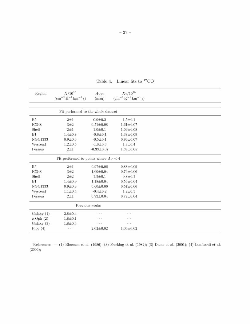
However, the 12CO emission saturates at AV ∼ 4 mag in every region, as shown in Figure 6.Therefore, we perform the estimation of the X factor in two ways: (i) for all the points, and (ii)for only those points with AV < 4 mag, where the column density can still be traced.

Figure 6 also shows that there is a threshold value of extinction below which no 12CO emissionis detected. To take this into account we fit the linear function

AV = AV 12 + X2W (12CO)9.4× 1020

, (18)

where AV 12 is the minimum extinction below which there is no 12CO emission and X2 is the slopeof the conversion (comparable to the X factor). The linear fit is performed using the bivariatecorrelated errors and intrinsic scatter estimator (BCES), which takes into account errors in bothaxes and provides the least biased estimation of the slopes (Akritas & Bershady 1996). The resultsof the X factor and the linear fits are presented in Table 4. In Figure 6, we show only the resultsfor points with AV < 4 mag: a dotted line for the standard X factor and a dashed line for thelinear fit.

The values derived for X using all the points (as previously done in the galactic determinationsof X) are in agreement with the mean value of (1.8 ± 0.3) × 1020 cm−2 K−1 km−1 s derived by

– 13 –

Dame et al. (2001) for the Milky Way. However, this fit is not good in the unsaturated regime(AV < 4 mag). Performing a linear fit to all of the data, including the saturated emission, cangive unreasonable solutions, such as a negative minimum extinction needed to produce 12CO (1-0)integrated intensity.

The linear fit performed to positions with AV < 4 mag gives the best estimate for the extinctionin the unsaturated regions but only provides a lower limit extinction estimate for the saturatedregimes, while the standard X factor provides a poor description of the data in both saturatedand unsaturated regimes. The histograms of the errors associated with the conversions derived forpositions with AV < 4 mag (bottom panels of Figure 6) show that the linear fit (open histogram)provides a more unbiased estimate of the extinction than the X factor (filled histogram). Thisimprovement in the precision of the extinction estimate goes along a reduction in the errors. Thewidth of a Gaussian fitted to the histograms of the regions implies a typical error of 40% and 25%for the X factor and the linear fit, respectively. Performing the same analysis on the histograms ofthe whole cloud gives an error of 59% and 38% for the X factor and the linear fit, respectively.

However, as we can see from Figure 6 the linear relation is not very accurate for AV > 4 mag.Therefore, following the simplest solution of radiative transfer

I = I0

(1− e−τ

),

we fit it to our data withW (12CO) = W0

(1− e−k(AV −Ak12)

), (19)

where W0 is the integrated intensity at saturation, Ak12 is the minimum extinction needed to get12CO emission, and k is the conversion factor between the amount of extinction and the opticaldepth. We perform an unweighted fit of the non-linear function to the data, which yield solutionsthat better follow the overall shape of the W (12CO) as a function of AV . Unfortunately, thebest fits for Westend and Perseus are quite poor and should be regarded with caution. The bestparameters are listed in Table 5 and are shown in Figure 6 as solid curves. We note that thethreshold extinction shows a large scatter, even in the more accurate non-linear fit. This suggeststhat different environmental conditions are causing the observed scatter (see § 7).

6.3. Using 13CO to derive H2 column densities

We expect the 13CO (1-0) transition to be optically thin at low extinction. If this is the case,a simple linear relation between the integrated intensity of 13CO and AV should fit the data,

AV = W (13CO) B13 + AW13 . (20)

The fit is done using the BCES algorithm for points with AV < 5 mag because there is somesaturation in the emission. The results are presented in Table 6 and in Figure 7. Once again, wefind that the minimum extinction needed to detect 13CO and the slope of the linear relation changes

– 14 –

between the regions, though the variation is smaller than with the 12CO data. From Figure 7 wecan clearly see the effect of saturation around 5 mag of extinction in IC348 and B1, similar to whatwas reported by Lada et al. (1994) in the more distant IC 5146, with comparable linear resolution.When comparing our results with the linear fit derived by Lada et al. (1994) we see that the fitparameters are quite different, suggesting that the IC 5146 cloud is quite different from Perseus.The linear fit for IC 5146 would indicate that for a region without extinction there is molecularemission, suggesting that the linear fit has been affected by points with saturated emission or thatthe fit errors are largely underestimated. Comparing our result for B5 with Langer et al. (1989),we find that the slopes are slightly different, but this can be reconciled by performing the linearfit taking all the points (B13 = 0.37 ± 0.1, AW13 = 1.45 ± 0.04) as done by Langer et al. (1989).However, the fit performed by Langer et al. (1989) was done using the extinction map derived byBachiller & Cernicharo (1986), that is limited by AV values below 5 mag of visual extinction (due toa lack of detectable background stars). Also, given that their molecular data has a better resolution(1.5′) than the extinction map (2.5′), they interpolated the 13CO to the extinction positions insteadof smoothing the data to the same resolution. Finally, the threshold extinction value differs fromprevious measurements mainly because it is hard to accurately define the zero point for extinctionmaps derived from optical star counting (as already mentioned, Schnee et al. 2005 reported adifference of ∼ 0.8 mag).

Following the column density determination shown in § 5.1, which takes into account the effectof optical depth and excitation temperature, we investigate the relation between N(13CO) and AV ,fitting a linear function to the data,

AV = N(13CO) c + AV 13, (21)

where c and AV 13 are the parameters of the fit. From the fit we can derive the ratio of abundancesbetween H2 and 13CO as [

H2

13CO

]= 9.4× 1020 c . (22)

The result for the fit over the whole cloud and by regions is shown in Figure 8, and in Table 7 wepresent the best fit parameters. When performing the fit we estimate the error associated with the13CO column density as 15%, due to the uncertainty in the calibration.

As shown in Figure 8, this relation presents a larger scatter, which is also present in individualregions (and it is consistent with previous work; see e.g. Combes 1991). As already pointed out,selective photodissociation and/or chemical fractionation can alter the simple linear relation atlow AV values, whereas optical depth may start to be large at high AV (see e.g. the tendency ofN(13CO) to flatten out at AV > 5 mag in B5, IC348 and B1).

The 13CO abundances derived from the fit present significant variations from region to region(see Table 7). We do not find a correlation between the abundance and the threshold AV 13. Thissuggests that 13CO abundance variations are mainly due to different chemical/physical propertiesin the inner regions of the cloud at AV > AV 13.

– 15 –

Comparing our results with those in Table 7, we see that the abundances agree very well,within the errors, with previous values reported in Perseus, taking also into account the ∼ 0.8 magdifference found by Schnee et al. (2005). This difference is produced by the difficulty in definingthe zero level of extinction, which is harder in the optical star counting method than using NICER.The extinction threshold derived for Perseus is close to the one derived for ρ-Oph by Frerking et al.(1982), but they do not have any data at AV below 2.5 mag and their determination has been doneonly for points with AV > 4 mag.

It is important to note that the numbers cited from previous works do not include the 10-20%calibration uncertainty that we do include in our results, and therefore our results are more accuratethan previous ones.

6.4. Using C18O to derive H2 column densities

We fit a linear relation between the integrated intensity of C18O and AV ,

AV = W (C18O)B18 + AW18 . (23)

The fit results are presented in Table 8 and in Figure 9. We find that, as in the case of 12COand 13CO, both parameters (extinction threshold and slope) vary between regions. However, dueto the fewer points available per region, the errors are larger than for previous fits.

Despite the small number statistics, we still can see that C18O is fairly linear up to at least10 mag. When comparing our results with the linear fit derived by Lada et al. (1994), we see thatthe fit parameters are quite different. However, they performed the fit over a wider AV range (upto 15 mag), and it is possible that despite their efforts the fit could have been affected by emissionwith higher optical depth.

Langer et al. (1989) derived a fit in B5. Unfortunately, we don’t have coverage for B5, andtherefore no direct comparison can be done. Nevertheless, we find that the threshold extinctionvalue derived for B5 is systematically lower than the values derived here for other regions (similar towhat is found in 13CO) while the slope is in agreement (within the error bars) with the parametersderived here.

6.5. 12CO (1− 0) Excitation Temperature vs. Extinction

Being collisionally excited, the excitation temperature of 12CO (1-0) is expected to increaseas we move from the outskirts of the cloud, where the extinction and volume densities may belower than the critical density for the 12CO (1-0) transition, to the most extinguished and densestregions, where 12CO (1-0) is in LTE and faithfully traces the gas kinetic temperature.

– 16 –

The excitation temperature, derived using 12CO and eq. 6, is shown as a function of the visualextinction in Figure 10. In addition we plot the median dust temperature computed in bins ofextinction as horizontal lines. When all the points are plotted (left panel of Figure 10) there is apoor correlation between excitation temperature and extinction. This is a direct result of mixingvery different environments within the cloud in one plot. In fact, from the right panel of Figure 10,where the excitation temperature and visual extinction are plotted for individual regions, it is clearthat the scatter is significantly lower and the excitation temperature rises from ∼ 5 K at low AV

(∼ 2 mag) up to a temperature close to the derived dust temperature in positions with AV > 4. Themore quiescent regions (B1 and B5) present a smaller dispersion, whereas more active regions (IC348and NGC1333) present a larger spread in the excitation temperature, probably because of the largervariation of physical conditions along the line of sight and/or the multiple velocity components. Theregion labeled as “Westend” has a very low excitation temperature when compared with the rest ofthe cloud. As shown in the right panel, in individual regions the dust temperature does not changemore than approximately one degree except in the “Shell” which shows a steady increase with AV ,and in NGC1333 where a peak of the dust temperature is present at AV ∼ 8 mag, probably dueto the internal heating produced by the nearby embedded cluster. On the other hand, the 12COexcitation temperature ranges between 5 and 20 K.

It is important to note that almost all the points lie below the median dust temperature of theregion, indicating that 12CO is tracing gas at volume densities well below 105 cm−3, the lower limitto have dust and gas coupling (Goldsmith 2001). The average excitation temperature for pointsabove 4 mag is 13.8 K, while the standard deviation is 2.3 K. We count the number of positionswhere the 12CO emission is sub-thermal (Tex < 11.5 K) obtaining that it is ∼ 60 %. Westend is aregion with 12CO excitation temperature always below the dust temperature. This could be due toa lower fraction of high density material compared to the other regions. It is interesting that in theregions in the North-East part of the cloud (B5, IC348 and Shell) the dust temperature is closerto 17 K while in the South-West part (B1, NGC1333 and Westend) it is closer to 16 K, suggestingvariations in the ISRF across the Perseus Complex.

7. Modeling using PDR code

To relate the observed variations in the 12CO and 13CO lines with changes in the physicalproperties of the regions, we use the Meudon PDR code (Le Petit et al. 2006)1. This code includesmost physical effects by explicit calculation; in particular it calculates the 12CO shielding, unlike themajority of other codes available (e.g. Rollig et al. 2007), where fitting formulae are used instead.

We use the abundances derived by Lee et al. (1998) (see table 9) for clouds with high metalabundances (more appropriate for the material traced by 12CO and 13CO) a 12C/13C abundance

1Available through http://aristote.obspm.fr/MIS/

– 17 –

ratio of 80 and a cosmic-ray ionization rate of ζ = 10−17 s−1 (a ζ value 6 times larger than theadopted one has also been considered, but found not to change the results by more than 10%; seeAppendix). To reproduce the observed [H2/13CO] ratio we increased the 12C abundance by a factorof 1.8 compared to Lee et al. (1998). To create curves of integrated intensity as a function of AV ,we run PDR models with different extinctions (AV = 0.5, 1, 1.5, 2, 2.5, 3, 4, 5, 8, 10 mag). Each PDRcalculation is performed over a grid of parameters, assuming a slab of constant density illuminatedon both sides: (1) The turbulent velocity is fixed to the Doppler parameter derived from the curveof growth fit assuming TR = 12 K for each region (see Table 3 and § 6.1). (2) The volume densityn = 103, 5×103, 104, 5×104 cm−3. (3) The radiation field is χ = 1 and 3 times the standard Draine’sradiation field (Draine 1978) (other χ values have been explored and reported in the Appendix).

The observed values of W (12CO), W (13CO) and W (12CO)/W (13CO) as a function of AV arecompared with the models results in Figure 11. To perform this comparison, the PDR code output,I =

∫Iνdν, is converted using the definition of brightness temperature (eq. 4):

W =∫

TR dv =I c2

2ν20k

c

ν0=

c3

2ν30k

I , (24)

and the ratio can be expressed as

W (12CO)W (13CO)

=(

ν(13CO)ν(12CO)

)3I(12CO)I(13CO)

(25)

First, we note that PDR models are reasonably good in reproducing 12CO and 13CO ob-servations, if one allows for variations in densities along different lines of sight. One exception isNGC1333, where the points with “excess” in 13CO emission are associated with positions just Southof the NGC1333 stellar cluster, where a second velocity component is observed. This produces lesssaturation in the 13CO emission. Secondly, in the case of 13CO, the Doppler parameter (shown inthe bottom panels of Figure 11) does not affect the results of PDR models within 10%, whereasfor 12CO, differences of ≤40% are present above 2 mag of visual extinction. In fact, the 12COline is optically thick, thus an increase in the line-width produces a significant increase in the linebrightness because of the optical depth reduction. The insensitivity of 13CO integrated intensityto variations of the turbulent line-width leaves the density and radiation field as the two possiblecauses of the observed differences between the regions.

In Figure 11 we show only the effects of density with χ = 1. Small variations (within a factorof 3) of the radiation field intensity slightly shift the curves to higher or lower AV by 1 mag, if theradiation field is larger or smaller, respectively. The main conclusions for individual regions arelisted below:

• B5: this is the most quiescent region in the whole Perseus complex. The best fit for theW (12CO) is a PDR model of a cloud with a narrow range of density change, between 5× 103

and 1×104 cm−3, values consistent with previous analysis. A similar density range is found to

– 18 –

reproduce W (13CO) at AV < 4 mag, whereas 5×104 cm−3 is more appropriate for the emissionat larger extinctions (higher density regions are mainly responsible for the 13CO emission atAV > 4 mag). We note that the integrated intensities of the two CO isotopologues approach(with increasing AV ) the lowest values in the whole sample, suggesting that denser materialis hidden to view because of photon trapping in the narrow range of velocities observed inthis region.

• IC348: in this cluster-forming region, the density spread is larger than in B5, with valuesranging between few × 103 and ' 1 × 104 cm−3. Similarly, the 13CO at low AV (< 4 mag)are reproduced by models with 103 − 104 cm−3, whereas densities larger than 5 × 104 cm−3

are needed above 4 mag. However, the points at AV > 7 mag and W (13CO) > 12 Kkm s−1

lie next to the embedded cluster, so that local heating and enhanced turbulence are probablyincreasing the 13CO brightness (the flattening of the W (13CO) vs. AV curve is in fact lesspronounced than in the case of B5, suggesting less optical depth). Thus, proto-stellar activityis locally affecting the 13CO emission, but not the 12CO.

• Shell: this region shows the largest spread in density for 12CO at all values of AV from1× 103 to about 3× 104 cm−3. At AV > 5 mag the data groups around two separate valuesof W (12CO): ∼ 35 and 55 Kkm s−1. The former group is associated with the (outer) shellreported in dust emission by Ridge et al. (2006b), whereas the latter is located in the innerpart of the shell, maybe exposed to a larger radiation field causing more dissociation of COmolecules. The 13CO emission appears similar to IC348, with the exception of points locatedat low W (13CO) (below 4 Kkm s−1) and AV > 4 mag which are again associated with theinner part of the Shell. This also suggests some further destruction process for the 12CO.

• B1: the 12CO emission is consistent with material at densities between 5×103−3×104 cm−3.Compared with B5, the B1 region shows brighter 12CO lines at lower (as well as higher)extinction. This is probably related to the larger Doppler parameter of B1. Several datapoints at low AV (<2 mag) are well reproduced by PDR models of dense clouds. The needof high densities at low AV also appears in the 13CO panel.

• NGC1333: this is the most active star forming site in the whole Perseus cloud and the be-haviour of the 12CO and 13CO integrated intensities as a function of AV is in fact significantlydifferent when compared to the other regions. First of all, the densities required in the PDRcode to match the data are mostly above 104 cm−3, both for the 12CO and 13CO emission.Secondly, the saturation of the 12CO line becomes evident only at AV > 6 mag (unlike∼ 4 mag, as in the other regions). Here, similarly to what is seen in B1, non-thermal motionsdriven by the embedded protostellar cluster are broadening the CO lines, allowing photonsfrom deeper in the cloud to escape. The effect is more pronounced than in B1, consistent withthe fact that NGC 1333 has the largest Doppler parameter among the six regions. We furthernote that, unlike in IC348, the 12CO (1-0) integrated intensity is also affected by the internalstar formation activity, significantly reducing the saturation and enhancing the brightness at

– 19 –

large AV . Internal motions, likely driven by protostellar outflows, are thus more pronouncedin NGC 1333 than in IC348, likely because of the larger star formation activity.

• Westend: this is the only region where no data points are present at AV > 6 mag, and the12CO, as well as the 13CO, integrated intensity shows a large scatter between AV of 1 and6 mag. These two facts are consistent with an overall lower density and probably clumpymedium, where relatively small high density clumps are located along some lines of sight,whereas a significant fraction of the data (19% of points in 12CO) can be reproduced byuniform PDR model clouds with densities below 5× 103 cm−3.

In general, model predictions for 13CO (1-0) can only reproduce well the observed emission atlow extinction (AV < 3 mag). The complex structure of active star forming regions, in particulardensity and temperature gradients as well as clumpiness along the line of sight (all phenomena notincluded in the PDR code) can of course contribute to the deviations from the uniform PDR models.We point out again that the largest Doppler parameters, i.e. the largest amount of non–thermal(turbulent?) motions, are present in active regions of star formation, so their nature appears tobe linked to the current star formation activity and not to be part of the initial conditions in theprocess of star formation.

In the bottom panel of Fig. 11, the W (12CO)/W (13CO) ratio is shown as a function of AV

for the six regions. The PDR models appear to reproduce well the integrated intensity ratio, for abroad range of AV . As we just saw, the 13CO data preferentially trace higher density material than12CO lines, so the black squares show the ratio between the 12CO and 13CO emission as predictedby PDR models with 5× 103cm−3 for 12CO and 1× 104cm−3 for 13CO lines. One thing to note inthese plots is the large fraction of points at low AV and low W (12CO)/W (13CO) which lie belowthe PDR model curves, in particular for B5, NGC 1333, and Westend, but they lie above theblack squares showing that the PDR model with different densities can reproduce all the emission.Another way to reproduce these data points is by decreasing the interstellar radiation field by afactor of a few. Alternatively, it is possible that these lines of sight intercept material where the13C carbon is still partially in ionized form, so that the reaction 13C+ + 12CO → 12C+ + 13CO+∆E(with ∆E/k = 37 K; Watson 1977) can proceed and enhance the 13CO abundance relative to 12CO.

We finally note here that Bell et al. (2006) have theoretically investigated the variation of theX factor using UCL PDR and Meudon PDR codes. They argue that variations in X can be due tovariations in physical parameters, such as the gas density, the radiation field and the turbulence,in agreement with our findings.

8. Summary and Conclusions

Using the FCRAO 12CO, 13CO and C18O data, and a NICER extinction map produced byCOMPLETE we perform a calibration of the column density estimation using 12CO, 13CO and

– 20 –

C18O emission in Perseus. We report the following results:

• We find a parameter space, VLSR(12CO)–Td, in which different spatial regions of the PerseusMolecular Cloud Complex also cluster, and we designate six regions within the complex (seeFigures 2 and 3). We note that the dust temperature decreases by about 1 K from NorthEast to South West.

• The 12CO data can be modeled with a curve of growth. The fit parameters vary betweenthe six regions and this causes much of the scatter in the W (12CO) vs. W (13CO) plot of thewhole Perseus Complex. The parameters derived from the fits agree with a previous study ofa sub-region of Perseus (B5) to within errors (see Figure 5).

• The X factor, X ≡ N(H2)/W (12CO), is derived from linear fits to the data both for thewhole Perseus Complex and for the six regions. The 12CO saturates at different intensitiesin each region, depending on the velocity structure of the emission, the volume density andradiation field. When the linear fit is done only for the unsaturated emission, the X factoris smaller than that derived for the Milky Way. However, larger values are obtained (closerto that found in the Milky Way) if all the points are included in the fit (see Figure 6 andTable 4). The most active star forming region in Perseus (NGC 1333) has the lowest X factorand the largest 13CO abundance among the six regions.

• The gas excitation temperature varies from 4 K to 20 K, it increases with AV , and it istypically below the dust temperature at all AV . This can be explained if a fraction (' 60%)of the 12CO (1-0) lines is sub-thermally excited, i.e. if the 12CO- emitting gas has volumedensities below ' 3× 103 cm−3.

• The column density of 13CO is derived taking into account the effect of optical depth andexcitation temperature. We find that the threshold extinction above which 13CO (1-0) isdetected is larger than has previously been reported. However, the fractional abundances(w.r.t. H2 molecules) are in agreement with previous determinations. The difference withprevious works is due to the superior zero-point calibration and larger dynamic range of theNICER extinction map, as compared to those derived from optical star counting (see Figure 8and Table 7).

• 13CO abundance variations between the regions do not correlate with the extinction thresholdAV 13, suggesting that the main cause of the variation is likely due to the chemical/physicalproperties of shielded molecular material deeper into the cloud. The 12CO (1-0) and 13CO (1-0) lines saturates at AV > 4, 5 mag, respectively, whereas C18O (1-0) line do not show signsof saturation up to the largest AV probed by our data (10 mag).

• Using the Meudon PDR code we find that the observed variations among the different regionscan be explained with variations in physical parameters, in particular the volume densityand internal motions. Large Doppler parameters imply large values of the CO integrated

– 21 –

intensities (as expected for very optically thick lines) and are typically found in active starforming regions (the largest values of the Doppler parameter and W (12CO) being associatedwith NGC 1333, the most active site of star formation in Perseus). On the other hand,quiescent regions such as B5 appears less bright in CO and only show a narrow range of COintegrated intensities as a function of AV . This is likely due to the fact that the photonsemitted from the higher density regions located deep into the cloud have similar velocitiesrelative to the outer cloud envelope traced by 12CO, so that they are more easily absorbed.Thus, turbulent (or, more generally, non-thermal) motions appear to be a by-product of starformation, more than part of the initial conditions in the star formation process.

This work has shown that local variations in physical conditions significantly affect the relationbetween CO-isotopologue emission and AV , contributing to the observed scatter. The use of astandard X factor, 1.8× 1020 cm−2 K−1 km−1 s, produces an overestimation of the cloud’s mass by∼ 45% when compared to the mass derived from the extinction map, while the lower limit for themass derived using the linear fit to the unsaturated points underestimates the mass by a ∼ 15%.The X factor (as well as the 13CO fractional abundance) depends on the star formation activity,with lower values associated with the more active (and turbulent) regions. Extinctions measured byusing 13CO and previous conversions from the literature are typically underestimated by ∼ 0.8 mag,so that more shielding is needed to produce the observed 13CO compared to previous findings.

JEP is supported by the National Science Foundation through grant #AF002 from the Asso-ciation of Universities for Research in Astronomy, Inc., under NSF cooperative agreement AST-9613615 and by Fundacion Andes under project No. C-13442. This material is based upon worksupported by the National Science Foundation under Grant No. AST-0407172. PC acknowledgessupport by the Italian Ministry of Research and University within a PRIN project.

A. Effect of χ and ζ variation

In Sect. 7 we have explored how changes in volume density and Doppler parameter affect the12CO (1-0) and 13CO (1-0) integrated intensities (W (12CO), W (13CO)) predicted by the MeudonPDR code. Here we show the effects of variations in the interstellar radiation field intensity, in unitsof Draine’s field (χ), and the cosmic-ray ionization rate (ζ) on W (12CO) and W (13CO). Fig. 12shows the results of this parameter space exploration in the particular case of B5 and volumedensity of 5 × 103 cm−3 (similar results apply to the other regions and different densities). Theupper panels display the model results for χ values of 0.5, 1, 5 and 10: the main change is visibleat AV < 4 mag, with a shift of the threshold extinction for 12CO and 13CO emission from about 1to 3 mag for an increase of χ from 0.5 to 10, respectively.

The cosmic-ray ionization rate used in the PDR models described in Sect. 7 is ζ = 1×10−17 s−1.This value is quite uncertain and Dalgarno (2006) suggests a higher rate of 6 × 10−17 s−1 for

– 22 –

molecular clouds (see also van der Tak & van Dishoeck 2000). In the bottom panels of Fig. 12, weshow the predicted W (12CO) and W (13CO) curves for ζ = 6× 10−17 s−1. The larger ζ value doesnot affect the CO emission at AV ≤ 3 mag, and only changes the integrated intensities by about30%. Thus, the effect is not large enough to explain the largest W (13CO) values.

REFERENCES

Akritas, M. G., & Bershady, M. A. 1996, ApJ, 470, 706

Alves, J., Lombardi, M., & Lada, C. J. 2007, In prep.

Arce, H. G., & Goodman, A. A. 1999, ApJ, 517, 264

Bachiller, R., & Cernicharo, J. 1986, A&A, 166, 283

Bell, T. A., Roueff, E., Viti, S., & Williams, D. A. 2006, MNRAS, 371, 1865

Bensch, F. 2006, A&A, 448, 1043

Bloemen, J. B. G. M., Strong, A. W., Mayer-Hasselwander, H. A., Blitz, L., Cohen, R. S., Dame,T. M., Grabelsky, D. A., Thaddeus, P., Hermsen, W., & Lebrun, F. 1986, A&A, 154, 25

Bohlin, R. C., Savage, B. D., & Drake, J. F. 1978, ApJ, 224, 132

Cambresy, L. 1999, A&A, 345, 965

Cernicharo, J., & Bachiller, R. 1984, A&AS, 58, 327

Combes, F. 1991, ARA&A, 29, 195

Dalgarno, A. 2006, Proceedings of the National Academy of Science, 103, 12269

Dame, T. M., Hartmann, D., & Thaddeus, P. 2001, ApJ, 547, 792

de Vries, H. W., Thaddeus, P., & Heithausen, A. 1987, ApJ, 319, 723

Draine, B. T. 1978, ApJS, 36, 595

—. 2003, ARA&A, 41, 241

Duvert, G., Cernicharo, J., & Baudry, A. 1986, A&A, 164, 349

Elias, J. H. 1978, ApJ, 224, 453

Frerking, M. A., Langer, W. D., & Wilson, R. W. 1982, ApJ, 262, 590

Goldsmith, P. F. 2001, ApJ, 557, 736

– 23 –

Goodman, A. A., Pineda, J. E., & Schnee, S. L. 2007, In prep.

Hatchell, J., & van der Tak, F. F. S. 2003, A&A, 409, 589

Hily-Blant, P., Pety, J., & S., G. 2005-1, CLASS evolution: I. Improved OFT support, Tech. rep.,IRAM

Lada, C. J., Lada, E. A., Clemens, D. P., & Bally, J. 1994, ApJ, 429, 694

Langer, W. D., Wilson, R. W., Goldsmith, P. F., & Beichman, C. A. 1989, ApJ, 337, 355

Le Petit, F., Nehme, C., Le Bourlot, J., & Roueff, E. 2006, ApJS, 164, 506

Lee, H.-H., Roueff, E., Pineau des Forets, G., Shalabiea, O. M., Terzieva, R., & Herbst, E. 1998,A&A, 334, 1047

Lombardi, M., & Alves, J. 2001, A&A, 377, 1023

Lombardi, M., Alves, J., & Lada, C. J. 2006, A&A, 454, 781

Miville-Deschenes, M.-A., & Lagache, G. 2005, ApJS, 157, 302

Padoan, P., Bally, J., Billawala, Y., Juvela, M., & Nordlund, A. 1999, ApJ, 525, 318

Ridge, N. A., Di Francesco, J., Kirk, H., Li, D., Goodman, A. A., Alves, J. F., Arce, H. G., Borkin,M. A., Caselli, P., Foster, J. B., Heyer, M. H., Johnstone, D., Kosslyn, D. A., Lombardi, M.,Pineda, J. E., Schnee, S. L., & Tafalla, M. 2006a, AJ, 131, 2921

Ridge, N. A., Schnee, S. L., Goodman, A. A., & Foster, J. B. 2006b, ApJ, 643, 932

Rieke, G. H., & Lebofsky, M. J. 1985, ApJ, 288, 618

Rollig, M., et al. 2007, A&A, 467, 187

Rohlfs, K., & Wilson, T. L. 1996, Tools of Radio Astronomy (Tools of Radio Astronomy, XVI, 423pp. 127 figs., 20 tabs.. Springer-Verlag Berlin Heidelberg New York. Also Astronomy andAstrophysics Library)

Schnee, S., Bethell, T., & Goodman, A. 2006, ApJ, 640, L47

Schnee, S. L., Li, J. G., Goodman, A. A., & Sargent, A. I. 2008, In prep.

Schnee, S. L., Ridge, N. A., Goodman, A. A., & Li, J. G. 2005, ApJ, 634, 442

Solomon, P. M., Rivolo, A. R., Barrett, J., & Yahil, A. 1987, ApJ, 319, 730

Spitzer, L. 1968, Diffuse matter in space (New York: Interscience Publication, 1968)

—. 1978, Physical processes in the interstellar medium (New York Wiley-Interscience, 1978. 333p.)

– 24 –

Strong, A. W., & Mattox, J. R. 1996, A&A, 308, L21

Tielens, A. G. G. M. 2005, The Physics and Chemistry of the Interstellar Medium (The Physics andChemistry of the Interstellar Medium, by A. G. G. M. Tielens, pp. . ISBN 0521826349. Cam-bridge, UK: Cambridge University Press, 2005.)

van der Tak, F. F. S., & van Dishoeck, E. F. 2000, A&A, 358, L79

Watson, W. D. 1977, in ASSL Vol. 67: CNO Isotopes in Astrophysics, ed. J. Audouze, 105–114

Wilson, R. W., Jefferts, K. B., & Penzias, A. A. 1970, ApJ, 161, L43+

Young, J. S., Goldsmith, P. F., Langer, W. D., Wilson, R. W., & Carlson, E. R. 1982, ApJ, 261,513

Young, J. S., & Scoville, N. 1982, ApJ, 258, 467

This preprint was prepared with the AAS LATEX macros v5.2.

Table 1. Clusters Regions Removed

Region Center R.A. Center Decl. Box Size(deg) (deg) (deg2)

IC 348 56.088 32.171 0.480×0.426NGC 1333 52.212 31.483 0.397×0.496

– 25 –

Tab

le2.

Typ

ical

Pro

pert

ies

ofth

eR

egio

nsfr

omA

vera

geSp

ectr

a

Reg

ion

W(1

2C

O)

Tm

ax(1

2C

O)

VL

SR

(12C

O)

σV

(12C

O)

W(1

3C

O)

Tm

ax(1

3C

O)

VL

SR

(13C

O)

σV

(13C

O)

Tex

τ(1

3C

O)

(Kkm

s−1)

(K)

(km

s−1)

(km

s−1)

(Kkm

s−1)

(K)

(km

s−1)

(km

s−1)

(K)

B5

83.2

9.8

40.9

01.6

0.9

99.9

90.6

412

0.3

1

IC348

93.0

9.0

11.1

82.2

0.9

38.9

90.9

512

0.3

5

Shel

l10

2.6

8.7

31.4

92.0

0.5

88.7

21.3

011

0.2

8

B1

12

2.6

6.7

11.5

51.6

0.9

96.8

30.9

911

0.3

3

NG

C1333

15

3.0

6.6

81.8

52.6

0.7

37.0

61.3

811

0.3

1

Wes

tend

10

2.2

4.2

01.9

62.0

0.6

54.5

81.1

99

0.4

4

Per

seus

11

1.7

7.2

62.6

52.2

0.3

97.6

72.1

511

0.3

4

Note

.—

W≡

inte

gra

ted

inte

nsi

ty.

Tm

ax≡

pea

kbri

ghtn

ess

tem

per

atu

re.

VL

SR≡

centr

oid

vel

oci

ty.

σV≡

vel

oci

tydis

per

sion

(=∆

v/√

8ln

2,w

her

e

∆v

isth

efu

llw

idth

at

half

maxim

um

).T

ex≡

exci

tation

tem

per

atu

reder

ived

from

12C

O.

τ≡

13C

Ooptica

ldep

th.

The

1-σ

unce

rtain

tyfo

rin

tegra

ted

inte

nsi

ty,pea

kbri

ghtn

ess

and

exci

tation

tem

per

atu

reis

estim

ate

dbet

wee

n15

and

30%

.

– 26 –

Table 3. Parameters for Growth Curve Fit

Region a TR b

(K−1 km−1 s) (K km s−1)

B5 0.61±0.03 20.5±0.5IC348 0.246±0.007 33.5±0.6Shell 0.223±0.009 40±1B1 0.33±0.01 36.8±0.7NGC1333 0.130±0.006 67±2Westend 0.44±0.03 24.7±0.9Perseus 0.260±0.004 35.9±0.4

– 27 –

Table 4. Linear fits to 12CO

Region X/1020 AV 12 X2/1020

(cm−2 K−1 km−1 s) (mag) (cm−2 K−1 km−1 s)

Fit performed to the whole dataset

B5 2±1 0.0±0.2 1.5±0.1

IC348 3±2 0.51±0.08 1.61±0.07

Shell 2±1 1.0±0.1 1.09±0.08

B1 1.4±0.8 -0.6±0.1 1.38±0.09

NGC1333 0.9±0.3 -0.5±0.1 0.93±0.07

Westend 1.2±0.5 -1.8±0.3 1.8±0.4

Perseus 2±1 -0.33±0.07 1.38±0.05

Fit performed to points where AV < 4

B5 2±1 0.97±0.06 0.88±0.09

IC348 3±2 1.60±0.04 0.76±0.06

Shell 2±2 1.5±0.1 0.8±0.1

B1 1.4±0.9 1.18±0.04 0.56±0.04

NGC1333 0.9±0.3 0.60±0.06 0.57±0.06

Westend 1.1±0.4 -0.4±0.2 1.2±0.3

Perseus 2±1 0.92±0.04 0.72±0.04

Previous works

Galaxy (1) 2.8±0.4 · · · · · ·ρ-Oph (2) 1.8±0.1 · · · · · ·Galaxy (3) 1.8±0.3 · · · · · ·Pipe (4) · · · 2.02±0.02 1.06±0.02

References. — (1) Bloemen et al. (1986); (3) Frerking et al. (1982); (3) Dame et al. (2001); (4) Lombardi et al.

(2006);

– 28 –

Table 5. Parameters for 12CO Fit

Region W0 k Ak12

(Kkm s−1) (mag−1) (mag)

B5 30.92 0.553 1.063IC348 39.27 0.350 1.374Shell 73.31 0.139 0.851B1 43.08 0.691 1.309NGC1333 67.12 0.374 0.748Westend 30.45 0.529 -0.160Perseus 42.29 0.367 0.580

Table 6. Results of Linear Fit to W (13CO)

Region AW13 B13 Reference(mag) (mag K−1 km−1 s)

B5 1.56±0.03 0.323±0.009 1IC348 1.99±0.03 0.36±0.01 1Shell 1.90±0.06 0.40±0.02 1B1 1.64±0.03 0.296±0.009 1NGC1333 1.19±0.03 0.26±0.01 1Westend 0.75±0.06 0.44±0.02 1Perseus 1.46±0.02 0.345±0.006 1

Previous works

IC 5146 -2.6±0.3 1.4±0.1 2B5 0.54±0.13 0.39±0.02 3

References. — (1) This work, linear fit for AV < 5; (2) Lada et al. (1994), linear fit for AV < 5;(3) Langer et al. (1989)

– 29 –

Table 7. Results of Linear Fit to N(13CO)

Region AV 13 c [H2/13CO] Reference(mag) (mag cm−2) ×105

B5 1.62±0.04 (4.0±0.2)×10−16 3.8±0.2 1,aIC348 2.15±0.04 (4.4±0.1)×10−16 4.1±0.1 1,aShell 2.23±0.05 (4.3±0.1)×10−16 4.1±0.1 1,aB1 1.68±0.04 (4.0±0.1)×10−16 3.8±0.1 1,aNGC1333 1.44±0.04 (3.0±0.1)×10−16 2.8±0.1 1,aWestend 1.19±0.05 (5.2±0.2)×10−16 4.9±0.2 1,aPerseus 1.67±0.02 (4.24±0.07)×10−16 3.98±0.07 1,a

Previous works

Perseus B5 0.5±0.1 (3.8±0.2)×10−16 3.6±0.2 2,bPerseus 0.8±0.4 (4.0±0.8)×10−16 3.8±0.8 3,bL1495 0.3±0.3 (4.5±0.6)×10−16 4.2±0.6 4,bL1517 0.3±0.5 (6±2)×10−16 5±1 4,bρ-Oph 1.6±0.3 (3.7±0.4)×10−16 3.5±0.4 5,cTaurus 1.0±0.2 (7.1±0.7)×10−16 6.7±0.7 5,c

Note. — (a) AV derived from NIR colors, (b) AV derived from star counting; (c) AV derivedusing spectra.

References. — (1) This work; (2) Langer et al. (1989); (3) Bachiller & Cernicharo (1986); (4)Duvert et al. (1986); (5) Frerking et al. (1982)

– 30 –

Table 8. Results of Linear Fit to W (C18O)

Region AW18 B18 Reference(mag) (mag K−1 km−1 s)

IC348 2.1±0.4 5±11 1Shell 2.7±0.3 4±7 1B1 2.1±0.1 2.5±0.9 1NGC1333 1.7±0.2 3±2 1Westend 1.6±0.3 3±5 1Perseus 2.4±0.1 2.9±0.9 1

Previous works

IC 5146 -0.7±0.3 10±1 2B5 1.40±0.22 1.8±0.13 3

References. — (1) This work; (2) Lada et al. (1994), linear fit for AV < 15; (3) Langer et al.(1989)

Table 9. Initial chemical abundances with respect to total Hydrogen

Element Abundance

He 0.1C+ 1.307× 10−4

13C+ 1.633× 10−6

N 2.14× 10−5

O 1.76× 10−4

S+ 8.00× 10−6

Fe+ 3.00× 10−7

– 31 –

0 2 4 6 8 10 12AV (mag)

0.15

0.20

0.25

0.30

0.35

0.40

0.45

σ(A

V)

(mag

)

Perseus

Fig. 1.— Error in the Perseus extinction map derived with NICER at each pixel versus the corre-sponding AV . Only the pixels used in this study are displayed here.

– 32 –

Fig. 2.— Central velocity compared with the dust temperature. Perseus is divided into six regionsthat are defined mainly in the space of physical parameters. This separation allows a betterunderstanding of the cloud.

– 33 –

03h50m0.00s 40m0.00s 30m0.00s 20m0.00s

Right Ascension (J2000)

29°

30°

31°

32°

33°

34°

Dec

linat

ion

(J20

00)

03h50m0.00s 40m0.00s 30m0.00s 20m0.00s

Right Ascension (J2000)

29°

30°

31°

32°

33°

34°

Dec

linat

ion

(J20

00)

0 2 3 5 7 8 10A V (mag)

Fig. 3.— (Top) The extinction map derived using NICER. The green border is the region observedin 12CO and 13CO (1-0) by COMPLETE, while the red border is the region observed in C18O (1-0) by Hatchell & van der Tak (2003). (Bottom) The re-gridded molecular data that fulfil therequirements detailed in § 3 are shown as boxes. Each of the defined regions are presented in adifferent color. B5 is green, IC 348 is magenta, the Shell is cyan, B1 is orange, NGC 1333 is blueand Westend is red.

– 34 –

0

1

2

3

4

TM

B (

K)

Perseus12CO

0.0

0.5

1.0

1.5

TM

B (

K)

Perseus13CO

0

1

2

3

4

TM

B (

K)

B512CO

0.0

0.5

1.0

1.5

TM

B (

K)

B513CO

0

1

2

3

4

TM

B (

K)

IC34812CO

0.0

0.5

1.0

1.5

TM

B (

K)

IC34813CO

0

1

2

3

4

TM

B (

K)

Shell12CO

0.0

0.5

1.0

1.5

TM

B (

K)

Shell13CO

0

1

2

3

4

TM

B (

K)

B112CO

0.0

0.5

1.0

1.5

TM

B (

K)

B113CO

0

1

2

3

4

TM

B (

K)

NGC133312CO

0.0

0.5

1.0

1.5

TM

B (

K)

NGC133313CO

-5 0 5 10 15velocity (km s-1)

0

1

2

3

4

TM

B (

K)

Westend12CO

-5 0 5 10 15velocity (km s-1)

0.0

0.5

1.0

1.5

TM

B (

K)

Westend13CO

Fig. 4.— Average 12CO (1-0) and 13CO (1-0) spectra for all Perseus and the six sub-regions.

– 35 –

0 5 10 15 20W(13CO) (K km s-1)

0

20

40

60

W(12

CO

) (K

km

s-1)

Perseus

0

20

40

60

W(12

CO

) (K

km

s-1)

B5 IC348

Shell

0 5 10 15 20W(13CO) (K km s-1)

0

20

40

60

W(12

CO

) (K

km

s-1)

B1

0 5 10 15 20W(13CO) (K km s-1)

NGC1333

0 5 10 15 20W(13CO) (K km s-1)

WestEnd

Fig. 5.— Integrated intensity of 12CO is plotted against the integrated intensity of 13CO. The leftpanel shows all data used while right panel shows each region separately, using the same colors asin Figure 3. The median of the 1-sigma errors are shown in bottom right of each plot. Solid linesare the growth curve fit, while the red curve in B5 is the fit from Langer et al. (1989).

– 36 –

0 2 4 6 8 10AV (mag)

0

20

40

60

W(12

CO

) (K

km

s-1)

Perseus

0

20

40

60

W(12

CO

) (K

km

s-1)

B5

IC348

Shell

0 2 4 6 8 10AV (mag)

0

20

40

60

W(12

CO

) (K

km

s-1)

B1

0 2 4 6 8 10AV (mag)

NGC1333

0 2 4 6 8 10AV (mag)

WestEnd

Fig. 6.— Top: Integrated intensity of 12CO and visual extinction derived using NICER. The leftpanel shows all data used and the right panel shows each region separately, using the same colorsas in Figure 3. Solid lines show the best fit of eq. (19), dotted and dashed lines are the standardW (12CO) X = N(H2) and straight line fits are only for points below AV =4, respectively. Bottom:Histograms of the difference between the observed and expected AV for all data displayed in toppanels. Filled and open histograms are for the standard X factor and linear conversion, shown asdotted and dashed lines in upper panels, respectively.

– 37 –

0 2 4 6 8 10AV (mag)

0

5

10

15

20

25

W(13

CO

) (K

km

s-1)

Perseus

0

5

10

15

20

25

W(13

CO

) (K

km

s-1)

B5

IC348

Shell

0 2 4 6 8 10AV (mag)

0

5

10

15

20

25

W(13

CO

) (K

km

s-1)

B1

0 2 4 6 8 10AV (mag)

NGC1333

0 2 4 6 8 10AV (mag)

WestEnd

Fig. 7.— Left panel shows 13CO Integrated intensity compared with the extinction. The medianof 1-sigma errors are shown in the bottom right corner of each plot. The best linear fit is shownwith a solid line. The right panel shows same plots as the left panel, but for the individual regions.

0 2 4 6 8 10AV (mag)

5

10

15

20

25

30

N(13

CO

) (1

015 c

m-2)

Perseus

5

10

15

20

25

30

N(13

CO

) (1

015 c

m-2)

B5

IC348

Shell

0 2 4 6 8 10AV (mag)

5

10

15

20

25

30

N(13

CO

) (1

015 c

m-2)

B1

0 2 4 6 8 10AV (mag)

NGC1333

0 2 4 6 8 10AV (mag)

WestEnd

Fig. 8.— The left panel shows 13CO column densities as a function of visual extinction. Themedian of the 1-sigma errors are shown in bottom right of each plot. The excitation temperatureis estimated using the 12CO peak temperature, assuming this transition to be optically thick. Thebest fit is shown with a solid line. The right panel show the same as the left panel, but separatedinto different regions.

– 38 –

0 2 4 6 8 10AV (mag)

0.0

0.5

1.0

1.5

2.0

2.5

3.0

3.5

W(C

18O

) (K

km

s-1)

Perseus

0.0

0.5

1.0

1.5

2.0

2.5

3.0

3.5

W(C

18O

) (K

km

s-1)

IC348

Shell

0 2 4 6 8 10AV (mag)

0.0

0.5

1.0

1.5

2.0

2.5

3.0

3.5

W(C

18O

) (K

km

s-1)

B1

0 2 4 6 8 10AV (mag)

NGC1333

0 2 4 6 8 10AV (mag)

WestEnd

Fig. 9.— The left panel shows C18O integrated intensities as a function of visual extinction. Themedian of 1-sigma errors are shown in the bottom right corner of each plot. The best linear fitis shown with a solid line. The right panel shows the same as the left panel, but separated intodifferent regions.

0 2 4 6 8 10AV (mag)

0

5

10

15

20

Tex

(K

)

Perseus

0

5

10

15

20

Tex

(K

)

B5 IC348 Shell

0 2 4 6 8 10AV (mag)

0

5

10

15

20

Tex

(K

)

B1

0 2 4 6 8 10AV (mag)

NGC1333

0 2 4 6 8 10AV (mag)

WestEnd

Fig. 10.— Excitation temperature derived using 12CO plotted against the visual extinction at thesame position. The median of the 1-sigma errors are shown in bottom right of each plot. The solidline is the median dust temperature for each sample within the extinction bin. The left panel showsall data used while the right panel shows them separated by regions.

– 39 –

0

20

40

60

W(12

CO

) (K

km

s-1)

B5 IC348

Shell

0 2 4 6 8 10AV (mag)

0

20

40

60

W(12

CO

) (K

km

s-1)

B1

0 2 4 6 8 10AV (mag)

NGC1333

0 2 4 6 8 10AV (mag)

WestEnd

0

5

10

15

20

25

W(13

CO

) (K

km

s-1)

B5 IC348

Shell

0 2 4 6 8 10AV (mag)

0

5

10

15

20

25

W(13

CO

) (K

km

s-1)

B1

0 2 4 6 8 10AV (mag)

NGC1333

0 2 4 6 8 10AV (mag)

WestEnd

0

10

20

30

40

W(12

CO

)/W

(13C

O)

B5b=1.7 km s-1

n=1 ×103

n=5 ×103

n=1 ×104

n=5 ×104

IC348b=2.8 km s-1

Shellb=3.3 km s-1

0 2 4 6 8 10AV (mag)

0

10

20

30

40

W(12

CO

)/W

(13C

O)

B1b=3.1 km s-1

0 2 4 6 8 10AV (mag)

NGC1333b=5.6 km s-1

0 2 4 6 8 10AV (mag)

WestEndb=2.0 km s-1

Fig. 11.— Results of the PDR modeling. Upper, middle and bottom panels show the comparisonbetween W (12CO), W (13CO) and the ratio W (12CO)/W (13CO) with AV , respectively. Black andgrey lines are derived from PDR models. Unconnected black squares show the ratio between 12COand 13CO emission predicted by the PDR model with densities of 5 × 103 and 1 × 104 cm−3,respectively.

– 40 –

0

20

40

60

W(12

CO

) (K

km

s-1)

B5b=1.7 km s-1

χ=0.5χ=1.0χ=5.0χ=10.

ζ=1 ζ=6

0 2 4 6 8 10AV (mag)

0

5

10

15

20

25

W(13

CO

) (K

km

s-1)

ζ=1

0 2 4 6 8 10AV (mag)

ζ=6

Fig. 12.— PDR results for the particular case of B5 and different values of χ and ζ (in units of10−17 s−1). Black solid, black dotted, gray solid and gray dotted lines show the PDR model resultsfor χ = 0.5, 1.0, 5.0 and 10 times the standard Draine’s radiation field, respectively. Variations inχ mainly affect the low AV emission, whereas different ζ values slightly change the emission valuesat AV > 4 mag.