co exchange between air and water in an arctic alaskan and...

CO2 exchange between air and water in an

Arctic Alaskan and midlatitude Swiss lake:

Importance of convective mixing

Werner Eugster,1 George Kling,2 Tobias Jonas,3 Joseph P. McFadden,4 Alfred Wuest,3

Sally MacIntyre,5 and F. Stuart Chapin III6

Received 14 June 2002; revised 9 January 2003; accepted 11 March 2003; published 24 June 2003.

[1] CO2 exchange between lake water and the atmosphere was investigated at ToolikLake (Alaska) and Soppensee (Switzerland) employing the eddy covariance (EC) method.The results obtained from three field campaigns at the two sites indicate the importance ofconvection in the lake in driving gas flux across the water-air interface. Measurementswere performed during short (1–3 day) periods with observed diurnal changes betweenstratified and convective conditions in the lakes. Over Toolik Lake the EC net CO2 effluxwas 114 ± 33 mg C m�2 d�1, which compares well with the 131 ± 2 mg C m�2 d�1

estimated by a boundary layer model (BLM) and the 153 ± 3 mg C m�2 d�1 obtained witha surface renewal model (SRM). Floating chamber measurements, however, indicated anet efflux of 365 ± 61 mg C m�2 d�1, which is more than double the EC fluxesmeasured at the corresponding times (150 ± 78 mg C m�2 d�1). The differences betweencontinous (EC, SRM, and BLM) and episodic (chamber) flux determination indicatethat the chamber measurements might be biased depending on the chosen samplinginterval. Significantly smaller fluxes ( p < 0.06) were found during stratified periods(51 ± 42mgCm�2 d�1) thanwere found during convective periods (150 ± 45mgCm�2 d�1)by the EC method, but not by the BLM. However, the congruence between averagevalues obtained by the models and EC supports the use of both methods, but ECmeasurements and the SRM provide more insight into the physical-biological processesaffecting gas flux. Over Soppensee, the daily net efflux from the lake was 289 ± 153 mgC m�2 d�1 during the measuring period. Flux differences were significant ( p < 0.002)between stratified periods (240 ± 82mgCm�2 d�1) and periods with penetrative convection(1117 ± 236 mg C m�2 d�1) but insignificant if convection in the lake was weak andnonpenetrative. Our data indicate the importance of periods of heat loss and convectivemixing to the process of gas exchange across the water surface, and calculations of gastransfer velocity using the surface renewal model support our observations. Future studiesshould employ the EC method in order to obtain essential data for process-scaleinvestigations. Measurements should be extended to cover the full season from thaw tofreeze, thereby integrating data over stratified and convective periods. Thus the statisticalconfidence in the seasonal budgets of CO2 and other trace gases that are exchanged acrosslake surfaces could be increased considerably. INDEX TERMS: 0315 Atmospheric Composition

and Structure: Biosphere/atmosphere interactions; 3307 Meteorology and Atmospheric Dynamics: Boundary

layer processes; 0322 Atmospheric Composition and Structure: Constituent sources and sinks; 1845 Hydrology:

Limnology; 1806 Hydrology: Chemistry of fresh water; KEYWORDS: carbon dioxide efflux, gas evasion from

lakes, CO2 flux, eddy covariance, turbulent mixing, water-atmosphere interactions

Citation: Eugster, W., G. Kling, T. Jonas, J. P. McFadden, A. Wuest, S. MacIntyre, and F. S. Chapin III, CO2 exchange between air

and water in an Arctic Alaskan and midlatitude Swiss lake: Importance of convective mixing, J. Geophys. Res., 108(D12), 4362,

doi:10.1029/2002JD002653, 2003.

JOURNAL OF GEOPHYSICAL RESEARCH, VOL. 108, NO. D12, 4362, doi:10.1029/2002JD002653, 2003

1Geographical Institute, University of Bern, Bern, Switzerland.2Department of Ecology and Evolutionary Biology, University of

Michigan, Ann Arbor, Michigan, USA.3Swiss Federal Institute for Environmental Science and Technology,

Dubendorf, Switzerland.

Copyright 2003 by the American Geophysical Union.0148-0227/03/2002JD002653$09.00

ACL 7 - 1

4Department of Ecology, Evolution, and Behavior, University ofMinnesota, St. Paul, Minnesota, USA.

5Marine Science Institute and Institute for Computational Earth SystemScience, University of California, Santa Barbara, California, USA.

6Institute of Arctic Biology, University of Alaska, Fairbanks, Alaska,USA.

1. Introduction

[2] The exchange of gases across the air-water interface ismediated by turbulence from wind shear, convection due toheat loss at the surface, rainfall, and microscale and large-scale wave breaking. All these processes induce turbulencenear the air-water interface, and turbulent eddies and theirassociated vorticity are required for gas fluxes to occur.Whileturbulence due to wave breaking induces large fluxes in theoceans, similar processes affect gas fluxes in lakes andoceans when wind speeds are between 3 and 8 m s�1. Atthese wind speeds, both microscale wave breaking, convec-tion in the water body, and wind shear contribute to aquaticturbulence. The few studies in lakes that consider high andmoderate wind speeds indicate that energy dissipation rates,which represent the magnitude of turbulence in the surfacewaters of lakes, are comparable to conditions in oceans[MacIntyre et al., 1999]. Below wind speeds of 3 m s�1,gas flux is independent of wind speed [Ocampo-Torres et al.,1994]. A number of empirical formulations have beenderived in order to describe gas flux, of which most arebased on wind speed [MacIntyre et al., 1995; Cole andCaraco, 1998; Wanninkhof and McGillis, 1999]. The contri-bution due to convection in the water is poorly understood.Convection is likely to be the dominant mechanism causinggas flux at low wind speeds. Energy budget analyses indicatethat current parameterizations will likely underestimate gasfluxes by a factor of two in tropical environments, whereevaporation is a major component of the surface energybudget [MacIntyre et al., 2001]. The contribution of heatflux has been included in one formulation for gas fluxes[Soloviev and Schluessel, 1994, 2001], but this was derivedfor the oceans and has not been satisfactorily applied to smalllakes [Anderson et al., 1999]. Lakes are often topographi-cally sheltered, affording them protection against strongwinds [Schladow et al., 2002; Kocsis et al., 1999], whichmakes the application of oceanographically derived formu-lations questionable under such conditions [Schladow et al.,2002]. Cole et al. [1994] showed that CO2 flux from smalllakes to the atmosphere can be a large component of thecarbon budget, and even of the surrounding landscape [Klinget al., 1991, 1992; Richey et al., 2002]. Therefore it isimperative that the processes controlling gas exchange withthe atmosphere are well understood and ultimately includedin parameterizations of the gas transfer velocity.[3] Over the past decade, the eddy covariance (EC)

method [e.g., Arya, 1988; Lenschow, 1995] has becomeestablished as the preferred approach for direct measure-ments of fluxes over terrestrial surfaces. Pioneer studiesemploying the EC technique have also been carried out toinvestigate trace gas exchange at the ocean surface [e.g.,Jones and Smith, 1977; Francey and Garratt, 1978; Weselyet al., 1982; Smith and Jones, 1985, 1986; Smith et al.,1991; McGillis et al., 2001] and across lakes [e.g., Edwardset al., 1994; Anderson et al., 1999]. However, EC measure-ments over lakes have so far shown significant disagree-ment with other techniques [see Anderson et al., 1999;Fairall et al., 2000]. Many of the studies of gas fluxes fromsmall water bodies have relied on floating chamber meth-ods, but these methods have been criticized [e.g., Belangerand Korzun, 1990; Stephens, 1978; Livingston and Hutch-inson, 1995]. It is these disagreements in methods and the

resulting uncertainties in both the actual CO2 flux and thespecific mechanisms responsible for the flux, which requirea comparison of methods and an analysis of the physicalprocesses controlling the flux of gas across the air-waterinterface [see also Fairall et al., 2000].[4] In this paper, we report measurements of two lakes in

which water-atmosphere fluxes of CO2, water vapor, andenergy were measured during periods with convectivemixing of the epilimnion: (1) during a cross-calibrationexperiment over Toolik Lake (Alaska), where floatingchamber and EC flux measurements were simultaneouslyperformed over four days in late July 1995 and on one dayin July 1994; and (2) in a subsequent field experiment inSeptember 1998 over Soppensee, a small lake in Switzer-land. For comparison, fluxes were also calculated from awind based model [Cole and Caraco, 1998] developed forsmall lakes and from a surface renewal model whichincorporates turbulence at the air-water interface [MacIntyreet al., 1995]. Flux measurements from both sites revealed acomplex pattern of gas flux which appears to be mainly aresult of the interplay of physical and biogeochemicalprocesses occurring in the atmosphere and in the lakes.During the study at Soppensee, wind speeds never exceeded3 m s�1. This data set allows us to examine the processesregulating gas flux in the absence of strong wind and withconditions of small waves.[5] A more comprehensive set of physical measurements

was obtained during the Soppensee experiment than atToolik Lake. Hence the Soppensee experiment is describedfirst as it provides insight into the Toolik Lake results from1995. The 1994 measurements at Toolik Lake were so shortthat they are only included in this paper for the purpose ofvalidation.

2. Sites, Data, and Methods

2.1. Sites

2.1.1. Toolik lake[6] Toolik Lake (68� 37.910N, 149� 36.320W, 719m a.s.l.)

is a small lake north of the Brooks range in Alaska. For thepast 25 years it has been the focus of arctic studies [O’Brienet al., 1997], being the site of the U.S. Arctic Long-TermEcological Research (LTER) station. Toolik Lake has asurface area of 1.5 km2, an average depth of 7 m, and amaximum depth of 25 m [O’Brien et al., 1997]. The maininlet to the lake provides an inflow of 125 � 103 m3 d�1,which is 71% of the total inflow [O’Brien et al., 1997](measured between 13 May and 31 August 1980). Thehigh dissolved organic carbon (DOC) concentrations (�5–7 mg L�1) reduce penetration of irradiance in the waterwith a typical attenuation coefficient of 0.5 m�1.[7] Dissolved inorganic carbon (DIC) fluxes in Toolik

Lake are dominated by river inflow and outflow, groundwa-ter inputs, and gas evasion to the atmosphere [O’Brien et al.,1997]. The river and groundwater inputs are supersaturatedin CO2 with respect to the atmosphere, and gas evasionaveraged �420 mg C m�2 d�1 during the open water periodof the year of about 100–120 days [Kling et al., 1991, 1992].2.1.2. Soppensee[8] Soppensee is a small holomictic eutrophic lake locat-

ed 20 km northwest of Lucerne, Switzerland (47� 05.460 N,8� 05.000 E, 596 m a.s.l.). It is about 800 m long and 400 m

ACL 7 - 2 EUGSTER ET AL.: CO2 EXCHANGE BETWEEN AIR AND WATER

wide with a surface area of 0.25 km2, and an average andmaximum depth of 12 m and 27 m, respectively. The lakedrains a 1.6 km2 catchment [Lotter, 1989; Gruber et al.,2000]. Soppensee has an outstanding record of varved sedi-ments that have allowed the reconstruction of the environ-mental history [Lotter, 1989] back to the last ice age. Thevarved sediments indicate very stable conditions of thesedimentation cycle and of the redox conditions. A strongthermal stratification generally develops in summer with arather constant epilimnion at about 3–4 m depth, and anoxicconditions in the bottom waters [Gruber et al., 2000].[9] A mass balance of the carbon cycle computed by

Gruber et al. [2000] indicates that most of the inflowcomes from groundwater which is, similar to Toolik Lake,supersaturated with respect to atmospheric CO2. The mod-eled annual CO2 efflux from Soppensee amounts to about164 mg C m�2 d�1 [Gruber et al., 2000]. While Soppenseeitself is surrounded by a narrow band of reed and forestvegetation, the largest fraction of the catchment area isintensely used for agricultural purposes.[10] In autumn, the season during which our field meas-

urements were taken, the surface inflow to and outflow ofDIC from Soppensee is almost zero, and the CaCO3-richground water is the main factor for the supersaturation of thesurface waters with DIC. The DIC concentration in the lakeis rather constant both in the epilimnion and the hypolimni-on, and it increases in the transition zone of the metalimnion[Gruber et al., 2000].

2.2. Eddy Flux Measurements

2.2.1. Instrumentation2.2.1.1. Floating Platforms[11] At Toolik Lake, for the 1995 experiment (27–31

July), we moored a platform near the center of the lake tohave equally good fetch for the EC system of at least 200 min all directions. The platform measured 2.42 � 6.10 m2,and consisted of two elements of equal size that wereattached to each other with a hinge in the middle. Thesurface of the platform was 0.38 m above the lake surfacewhen all equipment was loaded on the float. In 1994 (14–15 July), the instruments were mounted on the northern lakeshore, which required that data with mean wind directionfrom the land were excluded from the analysis.[12] At Soppensee (21–23 September 1998), we used a

much larger and more stable platform to further minimizethe influence of the oscillations observed in the time seriesrecorded at Toolik Lake. The size of this platform was 5 �7 m2, and it was mounted on two boats. Thus the surface ofthe platform was typically 0.80 m above the lake. Thepositioning of the platform was more critical than at ToolikLake because of the smaller size of Soppensee, and thetrees around the lake, representing significant roughnesselements that increase turbulence over the lake. The opti-mum mooring location was determined from ten years ofwind data from three automatic weather stations within 18km distance from the site. The expected fetch determinedby the distance to the shore was �440 m in the best case(with winds from the prevailing wind direction 300�), and�125 m in the worst case.2.2.1.2. Eddy Covariance Systems[13] The two EC systems used at both sites were com-

pletely different and will therefore be described individually.

At Toolik Lake, the set-up consisted of an ATI 3-D sonicanemometer and thermometer (Applied Technologies, Inc.,Boulder, Colorado, United States, model SAT-211/3Vx)operating at 10 Hz in 1994 and 20 Hz in 1995. Measure-ment height was 1.50 m and 1.62 m above the surface in1994 and 1995, respectively. A closed-path infrared gasanalyzer (IRGA) performed CO2 concentration measure-ments. A fast LI-COR 6262 instrument (LI-COR, Lincoln,Nebraska, United States) was used in 1994, providing 5 Hztime resolution, while in 1995 a LI-COR 6252 operating at a1-s time resolution was used. A brass tube (4 mm innerdiameter, 1 m long, wrapped with polyurethane insulationand reflective foil tape to minimize rapid temperaturefluctuations in the air stream) was positioned at a distanceof 15 cm from the center of the sonic anemometer’smeasuring volume. The air-sampling tube was connectedto the gas analyzer by �2.5 m of polypropylene tubing(3.2 mm inner diameter, Bev-a-line), and air was drawnthrough the system by a diaphragm vacuum pump at 8–9 Lmin�1. This rate was adequate to maintain turbulent flow inthe sampling tube and reduce limits on system bandwidthdue to the volume (11.9 cm3 of the gas analyzer cell;Leuning and King [1992], Suyker and Verma [1996], andLeuning and Judd [1996]). A 1-m vacuum hose between theIRGA and the pump was used to reduce the effect of high-frequency pressure fluctuations. The IRGA was calibratedwith zero air and a calibration gas standard (402 ppm,Matheson Gas Products, Montgomeryville, Pennsylvania,United States) under ambient conditions. The values werecross-validated against a LI-COR 6262 instrument; then, theLI-COR 6252 was attached to the pump, and the span wasadjusted in such a way that the concentration readingsmatched the LI-COR 6262 concentration readings. Finally,all data were post-calibrated for the present analysis withindependent concentration measurements performed using agas chromatograph (for details, see Kling et al. [2000]).CO2 concentration and flux values were multiplied by 1.078in this post-calibration step. This procedure was necessarybecause the LI-COR 6252 instrument has no pressurecorrection built in and therefore shows too low concen-trations when air is pulled through the instrument at therequired rate.[14] At Soppensee, we used a Solent HS 3-D research

grade sonic anemometer and thermometer (Gill InstrumentsLtd., Solent, U.K.) that operates at 100 Hz and provideserror-checked averaged measurements at 20 Hz temporalresolution. This instrument also has a built-in inclinometer,which allowed for the identification of any time periodwithin which the float had changed its position. However,the slow response of the inclinometer did not allow forinstantaneous corrections of high-frequency oscillations ofthe float. For CO2 and H2O measurements we used a NOAAopen-path IRGA [Auble and Meyers, 1992], which wasmodified to avoid moisture in the housing and to reducethe internal noise level using a 63 mF capacitor betweensignal and ground. The chopper wheel rotation speed was setto 30 Hz in order to provide the highest possible temporalresolution. The instrument was mounted 2.80 m above lakesurface, at a horizontal distance of 0.74 m from the center ofthe sonic anemometer’s sensor array. Neither pump nortubing were needed for this open-path instrumental set-up.The IRGAwas calibrated with a CO2-free gas and three CO2

EUGSTER ET AL.: CO2 EXCHANGE BETWEEN AIR AND WATER ACL 7 - 3

gas standards (318, 415 and 559.4 ± 2 ppm; Carbagas,Liebefeld, Switzerland). The H2O channel was calibratedwith a dew point generator in the Paul Scherrer Institute(Villigen, Switzerland), using seven dew point temperaturesbetween 0.85 and 18.81�C.2.2.1.3. Additional Measurements From Toolik Lake[15] Net radiation measurements (Rn) were performed

with a Fritschen-type net-radiometer [Fritschen, 1960] fromRadiation and Energy Balance Systems (REBS, Seattle,Washington, United States, model Q*6) and mounted at0.41 m above lake surface. A Davos-type net pyrradiometer[Ohmura and Schroff, 1983] from Swissteco (model S-1,Oberriet, Switzerland) was mounted at 1.62 m height. TheREBS instrument was intercalibrated with the Swisstecoreference instrument in the field at Happy Valley (69�070 N,148�500 W) on 18–19 June 1995, and new calibrationfactors for the REBS instrument were derived and usedthroughout the study. Because of unequal response to short-wave and long-wave radiation of the REBS instruments[Field et al., 1992; Whiteman et al., 1989], differentcalibration coefficients were used for Rn � 0 and Rn < 0.The Davos-type reference instrument was factory-calibratedbefore (19 October 1990) and after (16 September 1995) theintercalibration experiment at Happy Valley.[16] Air temperature and moisture at EC height was

measured with a Vaisala-type thermometer/hygrometer(Campbell Scientific, Logan, Utah, United States, modelHMP35C). At 0.39 and 0.46 m above the lake surface, airtemperature and moisture were measured with a home-builtaspirated psychrometer, which uses the AD592 integratedcircuit temperature sensor (Analog Devices, Inc., Norwood,Massachusetts, United States). One of the sensors was keptmoist with a wick. The psychrometer sensors were calibrat-ed at 0�C over a crushed ice-water bath and at 30�C in awarm water bath. Water temperature was measured atdepths of 0.005, 0.04, 0.14 and 0.34 m with platinumresistor sensors (REBS model STP-1). The wind profilewas measured with hot wire anemometers (TSI, Inc., St.Paul, Minnesota, United States, model 8470) at 0.66, 1.02,1.62 and 2.38 m a.g.l. with a ±3% accuracy in the range0–5.0 m s�1.[17] Radiation and meteorological sensors were polled

every 20 s by a data logger (model 21x, Campbell Scien-tific, Logan, Utah, United States) and averages wererecorded every 6 min.2.2.1.4. Additional Measurements at Soppensee[18] The CO2 concentration gradient was measured

between EC height and 0.30 m above the water surface witha LI-COR 6262 IRGA. The IRGAwas run in absolute modeand the inlets were switched by an automatic valve every30 s. Data from the first 10 s of each cycle were discardedin order to allow the sample cell to adapt to the change inconcentration. The sample flow rate was 5 L min�1.[19] Net radiation was measured with a Swissteco net

pyrradiometer (model S-1; Oberriet, Switzerland) at 0.42 mabove the water surface in order to minimize the influenceof the floating platform. The thin domes of the instrumentwere inflated with pressurized dry air, and the outer surfacewas kept dry by a steady air current over the domes. Thesampling cycle of the CO2 concentration gradient wascontrolled by a data logger (model CR10X, CampbellScientific Ltd., Loughborough, UK) which also collected

the data of the IRGA and the net pyrradiometer, therebyusing an internal averaging interval of 5 min.[20] Additional measurements were obtained from an

Aanderaa Instruments weather station (Bergen, Norway)equipped with a data logger and the following sensors: airtemperature and relative humidity in a radiation shield andcup anemometers at 0.5, 1, 2, and 5 m above lake surface;wind direction, buoy orientation, upward looking pyranom-eter and pyrradiometer sensors at 5 m; and downwardlooking pyranometer and pyrradiometer sensors at 0.5 m.A chain of thermistors assembled from Richard BranckerResearch (Ottawa, Canada) TR-1000 self-contained temper-ature logging units with 0.002 K resolution (absoluteaccuracy ±0.05 K) at depths of 0.5, 2.5, 4.5, 6, 7, 8, 9, 10,12, 17, and 25 m measured temperature in 2-s intervals. ANortek (Sandvika, Norway) 25� beam angle high resolutionacoustic Doppler current profiler (ADCP) operating at1.5MHz (resolution 0.1mm s�1; sampling frequency 0.5 Hz)was employed to measure water velocities between 3.3 and7.2 m depth using 40 vertical bins with 0.1 m spacing. ASeaBird (SBE-Electronics,Washington, D. C., United States)SBE 9/11 CTD profiler with an FP-07 fast response tem-perature probe (response time �15 ms at 0.1 mK resolution)was employed in a cable-constrained uprising mode at�0.08 m s�1 velocity. Data were collected at 96 Hz.2.2.2. Computations[21] The turbulent energy and CO2 fluxes in the vertical

direction above the lake surface were derived from thecovariances of the vertical wind speed w and the energycontent or CO2 concentration c,

Fc ¼ w0c0: ð1Þ

Fc is the vertical turbulent flux of entity c, the overbar denotesa temporal average (30 min were used for Toolik Lakedata, 5 min for Soppensee data according to section 3.1),and primes denote the instantaneous turbulent fluctuationsrelative to its temporal mean, e.g., w0 = w � �w. We use themicrometeorological sign convention with positive valuesfor w and vertical fluxes if they are directed away from thesurface toward the atmosphere, and negative values if thedirection is toward the surface. Ground heat flux is takenpositive when directed from the surface to the water body,and radiative fluxes are positive when directed toward thesurface.[22] The heat exchange between the lake water and the

atmosphere was computed from the CTD temperatureprofiles that were measured at 30-min intervals and thenfiltered over 6 consecutive profiles to eliminate apparentfluxes due to internal wave motion.2.2.3. Data Processing[23] Processing of the raw EC data included the following

steps: (1) removing spikes in the ATI sonic anemometerdata from Toolik Lake using an iterative two-sided filter thatremoves outliers outside the local 30-min average ±3s(where s is the standard deviation; the Solent sonic ane-mometer employed at Soppensee did not require thistreatment because its software does error checking andelimination internally); (2) quality check of 1-min averagedvalues of mean quantities and fluxes; (3) coordinate rotationof u, v and w wind components to align coordinate systemwith the stream lines of the 30-min averages [e.g., Zeman


and Jensen, 1987; McMillen, 1988; Kaimal and Finnigan,1994, pp. 235–239]; (4) determining time lag values forH2O and CO2 channels using a cross-correlation procedurethat finds the maximum absolute correlation within a timelag window of 0.5 t 2.0 s for each 30-min segmentof raw data; (5) de-trending sonic temperature, H2O andCO2 channels using a linear trend elimination procedure(see Rannik and Vesala [1999] for a discussion of linear de-trending versus auto-regressive filtering); (6) computingmean values and turbulent fluxes; (7) calibration of H2Oand CO2 fluxes to account for damping and high frequencylosses using the Eugster and Senn [1995] cospectral cor-rection model (see Horst [2000] for the validity of thisapproach and Massman [2000] and Massman and Lee[2002] for a similar approach); (8) correction of H2O andCO2 fluxes to account for the effect of concurrent densityfluctuations according to Webb et al. [1980].[24] For the final analysis, only those flux measurements

were used which were obtained during periods where themomentum flux was directed toward the surface. If themomentum flux is not downward, then all EC fluxesmeasured under such conditions are not expected to be adirect function of the local surface exchange processes. Thiscriterion eliminated 28% and 6% from our Toolik Lake andSoppensee data sets, respectively.

2.3. Floating Chamber Measurements

2.3.1. Instrumentation[25] Gas flux measurements were taken eight times dur-

ing the sampling period at Toolik Lake by means of afloating chamber. The clear Plexiglas chamber had an areaof 0.2 m2 and a headspace volume of �30 L. From theheadspace at least four headspace gas samples were takenduring the 60-min deployment. The gas samples wereanalyzed on a gas chromatograph with a thermal conduc-tivity detector. Water samples were also taken duringchamber employments, and analyzed for dissolved CO2

content on a gas chromatograph after a headspace equili-bration (see Kling et al. [2000] for further details).2.3.2. Computations[26] Gas exchange at the water surface was estimated

from the floating chamber using a time series of CO2

measurements in the chamber headspace. The fundamentalmodel of the change in gas concentrations (C) over time (t)in the headspace is given by

dC=dt ¼ �k Cmax � Cð Þ; ð2Þ

where k [s�1] is the gas exchange rate, and Cmax is themaximum concentration in the water; as C approaches Cmax,dC/dt approaches zero. The relationship

ln dC=dtð Þ ¼ ln k þ ln Cmax � C0ð Þ � kt; ð3Þ

involving the initial concentration in the headspace C0, wasfitted to the measurements using the least-squares techni-que. The variance in gas flux was taken as the standard errorof the model estimate of ln k + ln (Cmax � C0).[27] Overall fits to the model were good (r2 > 0.91) if

dC/dt was large (3 samples). However, in cases where dC/dtwas small (5 samples), the equation produced poor fits to thedata, and estimates of the slope and intercept were not

significantly different from zero (at p < 0.05). In these cases,a simple linear relationship of C(t) = a0 + a1t provided agood fit (r2 range of 0.85–0.98), and the slope a1 of thisrelationship (a1 = dC/dt) was used to estimate the change ingas concentration during the chamber employment. Overallgas flux (mg C m �2 d�1) was obtained by correcting thedC/dt values in the chamber headspace for the chambervolume and surface area. The variance in gas flux wastaken as the standard error of the model estimate of a1,which was corrected for chamber volume and surface area.[28] In two cases the concentration of CO2 in the chamber

decreased from one headspace measurement to another(�10–15 min apart); although this indicates an uptake ofCO2 by the lake water, the overall flux during these twoemployments (�60 min each) showed a net evasion fromthe lake to the atmosphere.[29] Gas flux was also estimated at Toolik Lake from

wind speed and measured differences between concentra-tions of CO2 in the surface water and in the atmosphere[Cole and Caraco, 1998]. Here we refer to this approach asthe boundary layer model (BLM). Convective mixing in thewater is not explicitly included in this model. We alsoestimated gas flux using a surface-renewal model (SRM)which includes both the effects of wind speed and heat lossat the air-water interface in its formulation [Crill et al.,1988; MacIntyre et al., 1995]. The turbulent velocity scalesdue to wind u

*wand heat loss w

*(the penetrative convec-

tion velocity scale according to Imberger [1985] and Dear-dorff [1970]) were obtained from a surface energy budgetcalculated as done by MacIntyre et al. [2002] using surfaceirradiances and wind speed obtained by the meteorologicalstation. This approach is based on Imberger [1985] with thecomputation of heat flux at the air-water interface includingthe penetration of irradiance into the mixed layer and below.Consequently, it accurately calculates the heating and cool-ing of the surface mixing layer in which turbulent mixingoccurs. The gas transfer velocity kSRM was calculated usingthe small eddy version of the surface-renewal model,kSRMSc

1/2 = c2u*wRet

�1/4, where kSRM is the gas transfervelocity, Sc is the Schmidt number, c2 is an empiricalcoefficient (0.56), u

*wis the turbulent velocity scale, and

Ret is the turbulent Reynolds number. The depth of thesurface mixing layer is the turbulent length scale. It isgenerally demarcated by temperature differences as smallas 0.01�C. Only one temperature profile was measured atToolik Lake during the field campaign, and it showed thedepth of the upper mixed layer was 3 m. The combinationof this profile, the surface meteorological data, and subse-quent time series studies of temperature at Toolik Lake from1998–2000 provide a basis for estimating the depth of themixing layer during a variety of meteorological conditionsat Toolik. During the initial period in which air temperatureswere much cooler than water temperatures, we used 3 m.During the second half of the experiment, when the air-water temperature differencewas less, we used a depth of 1m.When air temperatures exceeded lake temperatures as de-termined by the thermistors in the upper 0.34 m, we let themixing depth be 0.1 m. At Soppensee, we used a mixingdepth during convective conditions of 6 m, a depth based onprofiles of temperature gradients. During heating periods,we used a mixing depth of 1 m. These values must beconsidered as estimates representing relative conditions


within the measurement period and thus provide an under-standing of the physical processes occurring in the lake.Additional computational details are presented by MacIn-tyre et al. [2001, 2002].

3. Data Quality Assessment

3.1. Frequency Analyses

[30] Spectral and cospectral analyzes were used to controlthe proper operation and the time response of the individualinstruments and the flux measurements, respectively. Thew and c spectra at Soppensee exhibited throughout a patterncorresponding to the expected idealized spectra (Figure 1).The typical f �2/3 slope of the inertial subrange started atnatural frequencies beyond approximately 1 Hz, which wasgenerally well below the Nyquist-frequency of the mea-sured time series which was 10 Hz (see example spectra inFigure 1). Traces of white noise in the spectra begin to berelevant at f > 4 Hz (occasionally at f > 1 Hz). The H2Ochannel of the IRGA experienced a certain damping loss athigh frequencies which was much less pronounced in theCO2 channel of the same instrument. This damping is aresult of the additional 63-mF capacitor signal filter and theinternal anti-aliasing filter of the sonic anemometer’s analoginput channels. The overall damping constant of this set-upwas 0.30 s. This damping is not considered critical for ourflux measurements, since its behavior is well understoodand was corrected for using the approach by Eugster andSenn [1995; see also Horst, 2000].[31] Difficulties in measuring very small CO2 fluxes,

however, still remain. In addition to instrumental limitationsto resolve small fluctuations in CO2 concentration, theWebbet al. [1980] density flux can be much larger than the trueflux of CO2 [e.g., Leuning et al., 1982]. Webb et al. [1980]found that the true flux Fc of a scalar quantity is themeasured flux Fraw of that quantity plus an additive density

flux Fr , Fc = Fraw + Fr , where Fr is a function of thesensible and latent heat fluxes. This is certainly a problemfor open path IRGAs such as the one used at Soppensee [seeLeuning and Judd, 1996], but to a lesser extent for theclosed path IRGA used at Toolik Lake. Using the formulasuggested by Leuning and Moncrieff [1990] we estimatethat the tubing used at Toolik Lake reduced temperaturefluctuations by a factor 40 such that the Webb et al. [1980]density flux contribution is quite small, but nonzero becauseof moisture fluctuations. In cases where Fraw is small thesign of Fc could switch when Fr is added. This was the caseduring 10.9% and 30.8% of the time at Toolik Lake andSoppensee, respectively. We used this criterion to estimatethe 95% confidence intervals for CO2 fluxes that might notsignificantly differ from zero. This range was �0.0009 to0.0018 mg C m�2 s�1 at Toolik Lake and 0.0002 to 0.017mg C m�2 s�1 at Soppensee. Note that in the latter case wemeasured during a period where the water remained warmerthan the air at all times, such that Fr > 0. The signal-to-noiseratio of the IRGAs in use was less problematic (medianvalues of 92.5 and 172 were found at Toolik Lake andSoppensee, respectively).3.1.1. Determination of Averaging Timefor Soppensee Data[32] The cospectral analyses showed good correspon-

dence with the idealized cospectra (Figures 2 and 3). Theidealized cospectra scale with normalized frequency n,where n = f � z/�u [e.g., Panofsky and Dutton, 1984] isderived from the natural frequency f, the measurementheight z, and the mean horizontal wind speed �u. This goodagreement was found in all latent heat flux cospectra and theCO2 flux cospectra during periods with low variability ofthe CO2 flux. The only exceptions were found in the case ofCO2 flux during periods with high variability, althoughlatent heat flux cospectra were almost ideal (Figure 3).During such periods the lower frequencies of the cospec-trum were disturbed by low-frequency variations at n <0.0125 (Figure 4). By using Taylor’s frozen turbulencehypothesis and under the assumption of local stationaryturbulence conditions, this frequency scale can be translatedinto a wave number scale, k1 = 2 pf/�u [see Kaimal and

Figure 1. Power spectra of a 1-hour time segment of eddycovariance data collected at Soppensee between 4 and 5hours CET on 22 September 1998. The theoretical slopes ofthe inertial subrange are also given for undamped (/ f �2/3)and damped (/ f �8/3) spectra. High-frequency noise onlyappears in the spectrum of H2O and CO2 at frequencies>7 Hz. The sonic anemometer measurements do not showany signs of high-frequency noise.

Figure 2. CO2 flux cospectra from Soppensee duringperiods without convection in the lake. Composite of three1-hour cospectra (bold line; DOY 265, 12–13 and 15–17hours CET), and idealized undamped (thin dashed line) anddamped cospectra (thin solid line; damping constant 0.30 s;see Eugster and Senn [1995]).


Finnigan, 1994, p. 60]. To convert k1 into spatial wave-length scale, we used the relationship l = 2p/k1 [seePanofsky and Dutton, 1984, p. 74], yielding l = z/n,where l is the spatial wavelength in units of m. With z= 2.8 m, l of this low-frequency contribution is on theorder of 225 m, indicating that lower frequencies are mostlikely affected by the respiration occurring on land, aprocess which cannot directly be related to the CO2 exchangeprocess across the lake surface. Therefore we filtered theSoppensee fluxes by truncating the computation of thecovariance at f = 0.0033 Hz (n � 0.0125; dash-dottedvertical line in Figure 4) in order to eliminate the contribu-tion of CO2 flux that most likely originates from the landsurrounding the lake. This was done by averaging cova-riances over 5-min intervals, which were further block-averaged to 30-min values. It should however be noted thatthis procedure only captures �92% of the flux expectedover ideal terrain as can be determined by integrating theKaimal et al. [1972] cospectra from Kansas.[33] It is remarkable that in contrast to the CO2 flux

measurements (Figure 4), the vapor fluxes, measured withthe same combination of instruments, were nicely obeyingthe idealized cospectrum during these periods (Figure 3).3.1.2. Determination of Averaging Time for ToolikLake Data[34] In the case of Toolik Lake we used standard 30-min

averaging periods. The influence of the surrounding landsurface on the CO2 flux measurements (see Figure 5)appeared to be less problematic than at Soppensee. Thelow-frequency variation seen in Figure 5 is partially elim-inated from the covariance computations by using standard30-min averaging periods. It is expected that the clear gapbetween 0.001 < n < 0.035 separates flux contribution fromthe land (lower frequencies) from the ones that are related tothe lake surface exchange.3.1.3. Oscillations From Floating Platforms[35] In contrast to the measurement set-up on Soppensee,

the floating platform on Lake Toolik was much smaller.Therefore the oscillation of the float due to surface waves isclearly visible in the wind velocity spectra (Figure 6a). On

average, the extra variance introduced in the vertical velocitytime series is on the order of 6% of w02 and restricted to anarrow band of frequencies 0.7 < f < 1.2 Hz (Figure 6a).Although significant, this oscillation does not strongly influ-ence the cospectrum of the flux measurements (Figure 6b).Therefore we believe that there is no need for a special fluxcorrection to eliminate the traces of this oscillation. In thecase of the Soppensee data, the typical wind speed wasclearly lower than over Toolik Lake, and the floating plat-form was more rigid and larger, which reduced the effect ofoscillations to the variation normally observed in spectraldata. The motion contamination due to the gyroscopic effectsdescribed by McGillis et al. [2001] appear to be negligiblebecause of the relatively small perturbations in the lakecompared to the open ocean.

Figure 3. H2O flux cospectra from Soppensee duringperiods with largest CO2 efflux from the lake, composite ofthree 1-hour length data segments (bold line; DOY 265,01–02 and 20–21 hours CET; DOY 266, 21–22 hoursCET). The composite cospectrum closely follows theidealized damped curve at frequencies n > 0.2, indicatingthe high quality of the turbulent flux measurements.

Figure 4. As in Figure 3 but for CO2 flux. Vertical dash-dotted line indicates the cutoff of the 5-min high-passaveraging filter, which eliminates all fluctuations to the leftof that line.

Figure 5. CO2 flux cospectra from Toolik Lake duringperiods without convection in the lake. Composite of four1-hour cospectra (DOY 212, 00–01, 02–03, 04–06 ADT).Fluxes that are computed over standard 30-min intervalsintegrate all information to the right of the vertical dash-dotted line. The inset shows the details of the inertialsubrange slope with the expected undamped slope (solidline) and the damped slope (dashed line). Average z/�u was1.49 s.


3.2. Energy Budget Closure

[36] Good energy budget closure is generally consideredan indication of good quality flux measurement [Baldocchi,1994]. At Soppensee, the heat exchange across the waterinterface was determined by three independent methods: (1)as the residual term GEB-closure = Rn � H � LE asdetermined from the micrometeorological measurements,where Rn is net radiation, and H and LE are turbulentsensible and latent heat fluxes, respectively; (2) GmicT

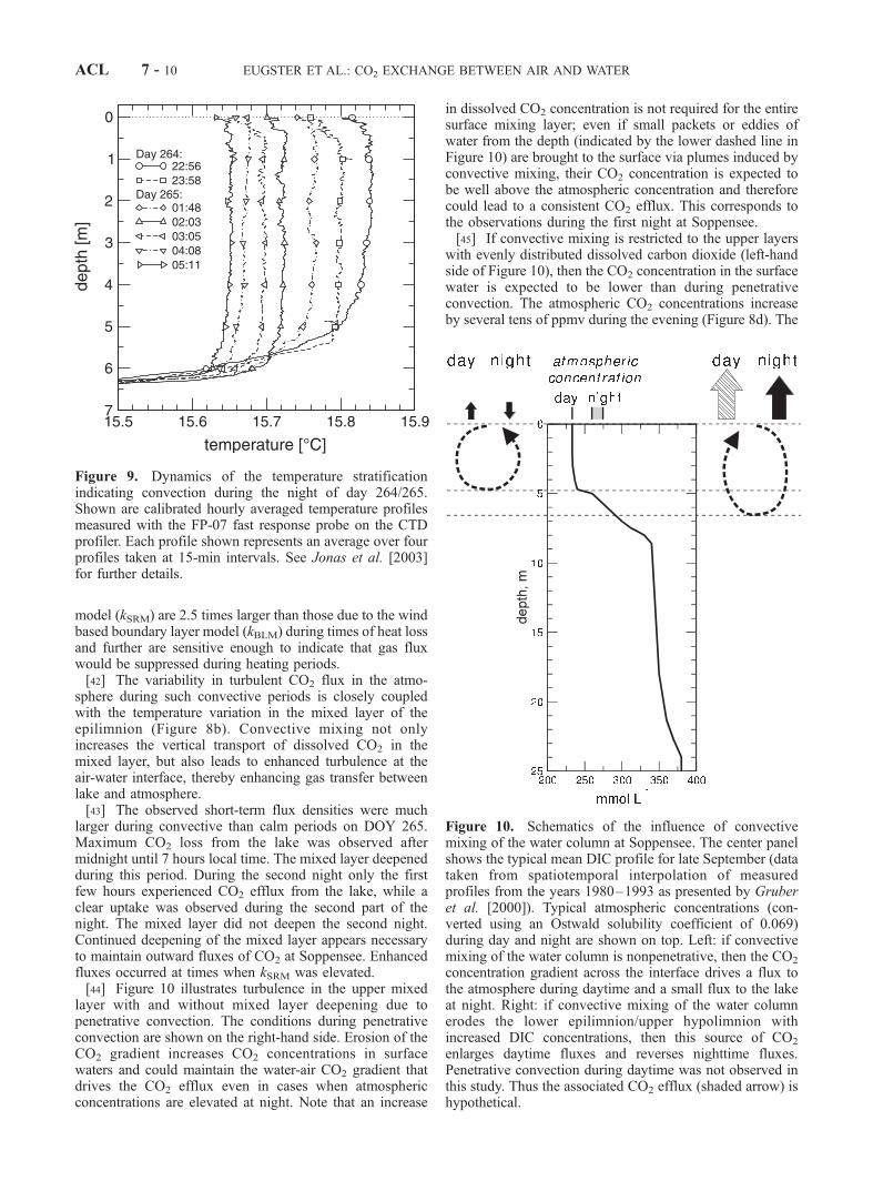
determined from the microstructure temperature profile inthe epilimnion including the penetration and entrainmentzone in the depth range 3.3–7.3 m; and (3) the heatexchange GT-chain determined from the temperatures of thearray of thermistors that were bin averaged for 5-minintervals and then filtered over ±4 hours. In theory weexpect GEB-closure = GmicT = GT-chain since they simplyrepresent the same variable determined in three independentways.[37] Figure 7 depicts the energy budget components for

the time period where measurements from all instrumentsoverlap. Here we use GmicT as a reference, against whichother methods should be tested. The general agreementbetween GmicT and GEB-closure is excellent, thereby confirm-ing the validity of the EC method. The average differencebetween GEB-closure and GmicT was <10 W m�2, with a slightbias toward GEB-closure > GmicT. The EC turbulent fluxmeasurements do not include advective flux components,which might be significant at this location and which maywell be of the same order of magnitude as the differencebetween GmicT and GEB-closure.[38] Overall, the energy budget data in Figure 7 indicate

that the EC flux measurements are of high quality. Inaddition to the quality control performed by using frequencyanalyzes, the agreement of the energy budget estimates alsoindicates excellent performance of the EC instruments.

4. Soppensee CO2 Exchange

[39] Our measurements from Soppensee indicate the ex-istence of two distinctly different regimes of CO2 exchange,

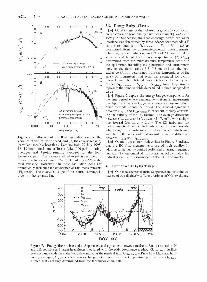
Figure 6. Influence of the float oscillation on (A) thevariance of vertical wind speed, and (B) the covariance w0T 0

v

(turbulent sensible heat flux). Data are from 27 July 1995,18–19 hours local time at Toolik Lake (100-point runningaverages and 5-point running averages for the low-frequency part). The variance added to w02 is restricted tothe narrow frequency band 0.7–1.2 Hz, adding �6% to thetotal variance. However, this float oscillation does notdramatically influence the covariance or flux measurements(Figure 6b). The theoretical slope of the inertial subrange isgiven by the separate line.

Figure 7. Energy fluxes observed at Soppensee, and agreement between methods. Rn: net radiation; Hand LE: sensible and latent heat fluxes measured with the eddy covariance method; GEB-closure: surfaceheat exchange with the water body determined as the residual term GEB-closure = Rn � H� LE, using half-hourly averages; GmicT: surface heat exchange determined from the temperature profiler data; GT-chain:surface heat exchange determined from the thermistor chain data.


illustrated by A and B periods in Figure 8. The A and Bperiods reflect the expected differences between calm con-ditions (A) with warmer atmosphere and thus stably strati-fied surface waters, compared to convective conditions (B)with colder air and the convective mixing of the epilimnion.A and B periods thus reflect the stratification in the lake, notin the air.[40] The A periods exhibited relatively smaller CO2

fluxes with very little variability (Figure 8a). The resultingnet flux was generally in the direction from the water tothe atmosphere, although individual 30-min flux averages(derived from 5-min covariances; compare section 3.1)showed either a zero net CO2 flux, or even a small CO2

uptake. Concurrent independent measurements of TR-1000temperature variation at 4.4 m depth (Figure 8b) andmicrostructure profiler temperature gradients (Figures 8cand 9) confirm the calm and stratified conditions in thewater during the A periods (further details on temperature

profiles in the lake will be presented by Jonas et al.[2003].[41] Epilimnetic temperatures had a high variance during

B periods (Figure 8b). In addition, the CTD profiler showedthat temperature gradients occurred frequently throughoutthe water column during these times (Figures 8c and 9). Thepresence of temperature gradients which reverse sign fre-quently, is indicative of turbulent mixing in the watercolumn [Imberger, 1985]. Rn was negative during B peri-ods, and wind speeds were low. Heat fluxes out of themixed layer occurred during B periods. Turbulent velocityscales in water due to heat loss (w*) are four times largerthan those due to wind forcing (u*w). Hence the mixing wasdriven by heat loss at the air-water interface. During bothnights (days 264/265 and 265/266) radiation fog formedwhich reduced long-wave radiative losses dramaticallyduring the second half of the night. The gas transfervelocities (data not shown) calculated by the surface renewal

Figure 8. Eddy covariance CO2 flux (a) measured above the surface of Soppensee (5-min fluxes blockaveraged over 30-min intervals) and independent measurements of: (b) the 15-min variance of watertemperature at 4.4 m depth; (c) temperature gradient in the depth range 4.5–7.0 m as measured with theCTD profiler, bin averaged upon 5-cm bins; (d) net radiation (bold line), GmicT from Figure 7 (dashedline), and ambient CO2 concentration (thin line); and (e) horizontal wind speed at 2.80 m height. The grayshade levels in Figure 8c are proportional to the vertical temperature gradient in K m�1 (negativenumbers indicate decreasing temperature with depth), and the white line corresponds to the lowerboundary of the convective aquatic layer (B periods), and of the remnant mixed layer (A periods),respectively. The surface water temperatures (not shown) varied between 15.3 and 16.9�C. Letter Adenotes times with low variance of the epilimnion temperature at 4.4 m depth, while B denotes times withsubstantially higher variance.


model (kSRM) are 2.5 times larger than those due to the windbased boundary layer model (kBLM) during times of heat lossand further are sensitive enough to indicate that gas fluxwould be suppressed during heating periods.[42] The variability in turbulent CO2 flux in the atmo-

sphere during such convective periods is closely coupledwith the temperature variation in the mixed layer of theepilimnion (Figure 8b). Convective mixing not onlyincreases the vertical transport of dissolved CO2 in themixed layer, but also leads to enhanced turbulence at theair-water interface, thereby enhancing gas transfer betweenlake and atmosphere.[43] The observed short-term flux densities were much

larger during convective than calm periods on DOY 265.Maximum CO2 loss from the lake was observed aftermidnight until 7 hours local time. The mixed layer deepenedduring this period. During the second night only the firstfew hours experienced CO2 efflux from the lake, while aclear uptake was observed during the second part of thenight. The mixed layer did not deepen the second night.Continued deepening of the mixed layer appears necessaryto maintain outward fluxes of CO2 at Soppensee. Enhancedfluxes occurred at times when kSRM was elevated.[44] Figure 10 illustrates turbulence in the upper mixed

layer with and without mixed layer deepening due topenetrative convection. The conditions during penetrativeconvection are shown on the right-hand side. Erosion of theCO2 gradient increases CO2 concentrations in surfacewaters and could maintain the water-air CO2 gradient thatdrives the CO2 efflux even in cases when atmosphericconcentrations are elevated at night. Note that an increase

in dissolved CO2 concentration is not required for the entiresurface mixing layer; even if small packets or eddies ofwater from the depth (indicated by the lower dashed line inFigure 10) are brought to the surface via plumes induced byconvective mixing, their CO2 concentration is expected tobe well above the atmospheric concentration and thereforecould lead to a consistent CO2 efflux. This corresponds tothe observations during the first night at Soppensee.[45] If convective mixing is restricted to the upper layers

with evenly distributed dissolved carbon dioxide (left-handside of Figure 10), then the CO2 concentration in the surfacewater is expected to be lower than during penetrativeconvection. The atmospheric CO2 concentrations increaseby several tens of ppmv during the evening (Figure 8d). The

Figure 9. Dynamics of the temperature stratificationindicating convection during the night of day 264/265.Shown are calibrated hourly averaged temperature profilesmeasured with the FP-07 fast response probe on the CTDprofiler. Each profile shown represents an average over fourprofiles taken at 15-min intervals. See Jonas et al. [2003]for further details.

Figure 10. Schematics of the influence of convectivemixing of the water column at Soppensee. The center panelshows the typical mean DIC profile for late September (datataken from spatiotemporal interpolation of measuredprofiles from the years 1980–1993 as presented by Gruberet al. [2000]). Typical atmospheric concentrations (con-verted using an Ostwald solubility coefficient of 0.069)during day and night are shown on top. Left: if convectivemixing of the water column is nonpenetrative, then the CO2

concentration gradient across the interface drives a flux tothe atmosphere during daytime and a small flux to the lakeat night. Right: if convective mixing of the water columnerodes the lower epilimnion/upper hypolimnion withincreased DIC concentrations, then this source of CO2

enlarges daytime fluxes and reverses nighttime fluxes.Penetrative convection during daytime was not observed inthis study. Thus the associated CO2 efflux (shaded arrow) ishypothetical.


combination of enhanced atmospheric concentration withlittle or no change in the water concentration could drive anair-water concentration difference that drives a net uptake ofCO2, which could explain the observed downward CO2 fluxon DOY 266. Although there is a weak positive relationshipbetween CO2 gradient measurements below EC height andEC fluxes, the accuracy of our gradient measurements wasnot sufficient to find significant correlations. 78% of ourCO2 gradient measurements were within an estimatedexperimental uncertainty of ±0.8 ppm m�1.[46] Convection in lakes occurs when heat losses exceed

heat inputs (G < 0). The transition from G > 0 to G < 0occurs in late afternoon and persists until next morning(Figure 8d). The largest fluxes of CO2 occurred at thosetimes, but the strongest effluxes of CO2 from the lake wereobserved during the first night of the experiment wherepenetrative convection occurred. A statistical unpaired two-sample t-test with unequal variances indicates that the meanflux of CO2 during A and B periods does not differsignificantly ( p = 0.76). The similarity occurs because bothupward and downward fluxes occurred during B periods,because mixed layer deepening did not always occur. WhenA periods are compared with B periods with penetrativeconvection (Bx in Table 1), differences in CO2 fluxes arehighly significant ( p < 0.002).

5. Toolik Lake CO2 Exchange

[47] Gas exchange at Toolik Lake is likely to be morecomplicated than at Soppensee because wind speeds werehigher, and heat losses also occurred through much of theexperiment and were likely to have contributed to fluxes(Figures 11c and 11d). The calculated heat fluxes (Figure 11c)indicate that the upper water column was likely to be stableonly at mid-day on days 208 and 209. At other times, heatlosses occurred. These were largest from late afternoon onday 208 until mid-morning on day 209 and for a similar

period the following day. Heating of the upper watercolumn occurred only during a brief period on days 210and 211. At mid-day on 211, the upper water columnfrequently shifted between heat losses and heat gains. Heatlosses from late afternoon to mid-morning were 4 timeslower on days 211 and 212 than during days 209 and 210.On the basis of these data, penetrative convection was morelikely on day 209 and 210 than on 211 and 212.[48] The increasing CO2 fluxes (Figure 11a) on DOY 209

section B suggests a correlation between efflux strength andthe convective mixing in the lake similar to the Soppenseedata. This efflux occurred even though the nocturnal CO2

concentrations in air were well above the daytime concen-trations (Figure 11b). However, because of the lack oftemperature profiler data, it is not possible to relate thegrowth of the convective mixing layer to the efflux patternobserved in the EC flux data.[49] During B periods on day 211, heat fluxes out of the

lake are low as are the measured gas effluxes. In contrast,gas fluxes are high early on day 212 when heat loss from thelake was similarly low. This indicates that strong heat losscausing penetrative convection at the lake surface is notrequired for a large gas efflux. Hence the Soppensee modelof Figure 10 does not necessarily also apply to arctic lakesin which CO2 concentrations in water exceed those in theatmosphere even at night.[50] Downward CO2 fluxes were observed from EC meas-

urements during A periods on day 209, 210, and 211. Surfaceheating (G > 0) occurred slightly before each of these fluxevents, and likely would have stratified the upper watercolumn. A transition to heat loss from the lake occurred justprior to and during these downward fluxes (Figure 11c), andwould have created a shallow mixing zone in which theturbulence created could be used to support CO2 fluxes intothe lake. However, measured CO2 concentrations in the lakewere always higher than atmospheric concentrations, andthus these downward fluxes are anomalous with respect tothe observed CO2 gradient. One possible explanation is that adownward CO2 flux occurred at measurement height, but didnot reach the lake. Because this is only likely duringextremely stable atmospheric conditions, we examined theMonin-Obukhov stability parameter z/L in the atmosphereand found that during each period of downward CO2 flux,and only during those periods, z/L was positive whichindicates a more stable atmosphere (data not shown). At allother times z/L was negative and indicated good mixingconditions in the atmosphere.[51] The CO2 fluxes during A periods were statistically

lower than during B periods at the p < 0.06 level. Both theboundary layer model and the surface renewal model showfluxes out of the lake during the entire period and do notshow the large fluxes that occurred on day 209 and day 212.However, average fluxes obtained from these calculationsand the EC measurements are similar (131 ± 2, 153 ± 3, and114 ± 33 mg C m�2 d�1 for BLM, SRM, and EC,respectively). Chamber measurements were higher thanEC, BLM, and SRM approaches during the heating periodon day 208, but were similar to BLM and SRM calculationsat all other times.[52] Figure 12 shows the dependency of CO2 fluxes as a

function of the air-water temperature difference �T (r2 =0.387, p < 0.001) with a slope of �57 to �84 mg C m�2

Table 1. Daily Net CO2 Exchange at Soppensee (in 1998) and

Toolik Lake (in 1995) as Measured With the Eddy Covariance

Method and the Floating Chamber Method and Determined by

Model Calculationsa

Net CO2 Flux

Soppensee Toolik Lake

N CO2 Flux N CO2 Flux

A: stratified periods 33 240 ± 82 59 51 ± 42B: convective periods 54 319 ± 242 105 150 ± 45Bx: very convective periodsb 35 1117 ± 236 – –A + B: total net flux 87 289 ± 153 164 114 ± 33Floating chamberc – – 8 365 ± 61Concurrent EC fluxd – – 16 150 ± 78Boundary layer modele – – 602 131 ± 2Surface renewal modelf – – 597 153 ± 3Model calculationg – 164 – –

aCO2 flux values are given in mg C m�2 d�1 (mean ± standard error). Ndenotes number of 30-min averages in this case.

bExcludes the period DOY 265.95–266.42.cAverage of eight 1-hour chamber deployments.dAverage of sixteen 30-min EC flux averages matching the times of

floating chamber deployments.eBoundary layer model [Cole and Caraco, 1998] computed at 6-min

resolution for the full period.fComputed as done by MacIntyre et al. [2002] at 6-min resolution for the

full period.gAnnual mean [Gruber et al., 2000].


d�1 K�1 (95% confidence interval) and an intercept between�39 and +70 mg C m�2 d�1. This relationship is notexpected to be universal since it implicitly also representsthe difference in CO2 concentration across the air-waterinterface. However, it indicates a possible relevance ofconvective mixing of the epilimnion for CO2 fluxes overlakes if �T is an indicator of the rate of mixing in theepilimnion.[53] The 1994 flux measurements (Figure 13) confirm the

importance of convective mixing for CO2 efflux with a clearanti-correlation between CO2 flux and the air-water temper-ature difference.

6. Discussion

[54] Over ocean surfaces, there is a high degree ofhorizontal homogeneity of surface roughness and hence ofthe mechanically-induced turbulent flow field. In contrast,most lakes are well embedded within a terrestrial environ-ment, with which they are strongly interacting [e.g., Kocsiset al., 1999; Schladow et al., 2002]; and the atmosphericconditions near the lake’s surface are only partially deter-mined by the exchange processes that occur over the lakeitself. From the standpoint of regional and local meteorol-ogy, the fractional cover of the lakes examined in this paperis small compared to the terrestrial surface surroundingthem. Therefore atmospheric conditions are largely deter-mined by the land-surface processes, onto which the lake-

surface processes superimpose a local anomaly. For exam-ple, during daytime a lake may be a cold spot in thelandscape, whereas it is a hot spot at night [see also Sunet al., 1998]. However, the cold lake surface during daytime

Figure 11. CO2 fluxes (reported in carbon flux units) observed over Toolik Lake: (a) eddy covarianceCO2 flux measurements (open circles: 30-min averages; bold line: 9-point running average), boundarylayer model fluxes calculated with the Cole and Caraco [1998] model (dashed line), and floatingchamber fluxes (squares; with standard error bars); (b) atmospheric CO2 concentrations (solid line: fromeddy covariance system; squares: syringe samples analyzed in gas chromatograph); (c) net radiation (thinline) and heat exchange G across air-water interface (bold line); and (d) horizontal wind speed. The datain Figures 11b–11d are 6-min averages. Letters A and B denote stable (G > 0) and convective (G 0)conditions in the epilimnion, respectively. Time is recorded as ADT and the daily solar maximum andminimum occur at 14 and 2 hours ADT, respectively.

Figure 12. Correlation between the CO2 flux over ToolikLake and the temperature difference across the air-waterinterface as measured between 0.39 m above and 0.005 mbelow the lake surface. The solid line is the linear best fit,and the dashed lines indicate the 95% confidence interval ofthe fit.


does not necessarily imply that the atmosphere above it isstably stratified; turbulent eddies nourished by the heat fluxfrom a nearby warm land surface are large enough toimpose turbulent and unstable conditions over the cold lakesurface. At Toolik Lake, for instance, the atmosphericsurface layer was unstable (z/L < 0) during 71% of the timewhile �T across the air-water interface was negative onlyduring 66% of the time (during the Soppensee experimentz/L indicated unstable atmospheric conditions at all times).At night, heat exchange across the warm surface keeps thenear-surface layer above the lake unstably stratified, butcold, potentially moist and CO2-rich air is advected from theupwind lake shore onto the surface, leading to potentiallyrapid increases in atmospheric CO2 concentrations at night.These are not a result of local outgassing of CO2 from thelake, but could significantly modify the flux across the air-water interface via the change in CO2 gradient. This is incontrast to open ocean conditions where the atmosphericconcentration is assumed constant.[55] Another important difference between CO2 fluxes

over oceans and over lakes is related to the proximity ofCO2 sources. The ultimate source of CO2 may be linked toorganic matter in the sediments or the influx of CO2-richgroundwater into the lake, and all but the largest anddeepest lakes are closer to these sources than are the oceans.In addition, regardless of the ultimate source of CO2, theproximate source is most often related to the patterns ofvertical stratification in the lake. The differences in CO2

concentrations between surface and metalimnetic or bottomwaters are usually higher in lakes than in oceans, and thephysical separation between such low versus high zones ofCO2 is lower in lakes than oceans (i.e., thermocline depthsare shallower in lakes). Given these general differences inphysical and chemical characteristics, a given input of

mixing energy will more often tap into sources of CO2-richwater in a lake than in an ocean. The measurements fromSoppensee illustrate how important penetrative convectionis, especially in regards to the striking difference betweenthe CO2 efflux observed early on DOY 265 versus the CO2

flux in the opposite direction early on DOY 266. In additionto the correlations of convective mixing and increased CO2

flux, evidence of a physical mechanism is provided for bythe pattern of surface currents observed with the ADCP inSoppensee. The patterns indicate strong downward plumeswith a characteristic core diameter on the order of 5 m[Jonas et al., 2003] during the night. During the day,vertical velocities were typically below 1 mm s�1 and didnot exhibit much structure [Jonas et al., 2003].[56] The great variability of EC CO2 fluxes, especially

during periods with convective mixing of the epilimnion, isconsistent with the operation of such plume structures in achemically stratified water body. Footprint estimates of theEC flux measurements were performed using the Schmid[1997] source area model. The footprint is defined as thesurface area upwind from the EC instruments that directlyinfluences the magnitude of the observed fluxes. If thefootprint is completely over the lake surface, then advectiveinfluences from the land do not significantly contaminatethe EC measurements. However, if the footprint includes arelevant proportion of the land, then the EC flux measure-ments are no longer representative for the lake surfacealone. On Soppensee the characteristic dimensions of thesurface area that contributes 90% to the total flux measure-ment under unstable conditions was as follows: The instru-ments do not ‘‘see’’ the surface closer than 15 m from themast; the point of maximum contribution is roughly 45 mupwind; the far end of the 90% isoline is at 120 m upwind(thus still within the nearest distance to the shore which was

Figure 13. Eddy covariance flux measurements during the 1994 Toolik Lake experiment. (a) CO2 flux;(b) atmospheric CO2 concentration; (c) net radiation (thin line) and temperature difference measuredbetween 1.5 m above and 0.05 m below the lake surface (thick line); (d) horizontal wind speed.Averaging time is 30 min.


125–440 m away); and the maximum width of the footprintis 16 m (values computed for z = 2.8 m, z0 = 0.001 m, z/L =�0.2, and sv/u* = 1.5; the z0 and sv/u* estimates werederived from our measurements). These values indicate thatthe flux measurements from Soppensee during convectiveperiods (where both the epilimnion and the atmosphericsurface layer are convective) integrate over a lake surfacearea that contains a few plumes only. Therefore we hypothe-size that some of the observed EC flux variability could becaused by significant differences in the plume-related ver-tical CO2 fluxes in the epilimnion. In this case we wouldexpected that the atmospheric turbulence and stability aswell as the diurnal cycle of CO2 concentrations in air are themost relevant factors governing the physics of gas exchangeat the water surface, in addition to the availability of thesevariable and intermittent sources of CO2. The 90% footprintarea at Toolik Lake for similar conditions extended between6 and 52 m upwind with a maximum contribution fromroughly 20 m upwind. With increasing stability the foot-prints in both cases grow larger than the values given here.[57] Footprint modeling is however still a controversial

issue. Although the Schmid [1997] model yields similarvalues for the point of maximum contribution as theSchuepp et al. [1990] model, the assumptions for thetrailing end of the footprint and thus for the potentialcontribution of the land surface to fluxes measured overthe lake are not identical. Schmid [2002] provides a thor-ough review of various footprint calculations and addressestheir limitations and weaknesses. Figure 14 illustrates theproblem for CO2 flux measurements over small lakes duringnocturnal conditions where the lake is warmer than thesurrounding land surface and wind speeds are near calm.Within an internal boundary layer (IBL) a local circulationbetween the land and lake is expected to transport CO2

originating from terrestrial ecosystem respiration to the lake[see Sun et al., 1998, 2001]. At the same time, CO2 is mixedabove the lake surface, is exchanged between atmosphereand the lake, and is mixed in the lake by convection,potentially eroding CO2-rich waters at depth when convec-tion is penetrative. Since EC measurements are not made at

the surface but at some height above it, the flux from thelake surface must be separated from the advective flux fromthe land/lake interaction. Our approach was to use shorteraveraging times for covariances at Soppensee which acts asa high-pass filter that is supposed to eliminate contributionsfrom larger eddies that are most likely associated with theexchange between land and lake. At the same time, it isobvious that by reducing the averaging time we also misssome low-frequency contributions that are not related toexchange processes between land and lake. In future studieswe suggest to measure even closer to the surface than wedid, provided that the IRGA has a shorter optical path lengthand is capable of at least 20 Hz temporal resolution. Thisshould increase the confidence that the EC flux is notsignificantly influenced by land/lake interactions. Thetrade-off is the larger loss on the high-frequency end ofthe flux cospectra. The gain at the low-frequency end of thecospectra appears to be beneficial despite the increase inhigh-frequency losses.[58] Biological processes were not treated explicitly in this

study. It should therefore be kept in mind that photosynthesisduring daytime and respiration during nighttime also influ-ence the CO2 concentrations in surface waters, therebyacting as a local sink during the day and a source duringthe night. However, the great variability in CO2 flux that isonly observed during convective (nocturnal) periods but notduring daytime strongly indicates that biological processesalone cannot explain the observed differences in gas fluxesbetween convective and nonconvective conditions.[59] Profiles of dissolved CO2 concentrations in Toolik

Lake are unavailable for the 1995 campaign, but typicalprofiles in July show surface values of �20–30 mM CO2

and values at the base of the metalimnion (�8 m depth) of50–60 mM. Such differences indicate the potential forpenetrative convection to tap into CO2-rich water and bringit to the surface, thus enhancing both the variability andmagnitude of CO2 flux to the atmosphere. Although mixingto 8 m depth was improbable during our study period, laterin the season when heat losses are greater, even highereffluxes are likely.

Figure 14. Processes influencing the eddy covariance (EC) flux measurements above a lake surface atnight. Because EC measurements cannot be performed directly at the air-water interface, the CO2

exchange with the lake (blue and red arrows) at EC reference height (black dash-dotted line) is measuredtogether with the exchange flux of CO2-rich air from the land surrounding the lake (pink and yellowarrows) where CO2 originates from respiration of soils and vegetation (black arrows). This local lake-breeze type circulation is expected to be restricted in its vertical extent by an internal boundary layer(IBL). See color version of this figure at back of this issue.


[60] The flux footprint areas were smaller over ToolikLake than over Soppensee because of the lower instrumentheight. The small footprint may have contributed to the highvariability of 30-min flux averages. The chamber measure-ments and BLM and SRM models always indicated a netefflux out of the lake, whereas the EC measurementssometimes indicated fluxes into the lake. While the bulkmeasurements of CO2 concentrations in the lake indicatethat fluxes should be outward, if surface waters were stablystratified, biological activity could draw down CO2 concen-trations and lead to lower values in a thin layer near the air-water interface [Soloviev et al., 2001]. While the chambersalways measured an efflux integrated over their full deploy-ment (�60 min), during two partial periods of measurementwithin two different deployments the CO2 concentration inthe chamber decreased, indicating an uptake of CO2 by thelake. These periods of measurement occurred during the Aperiod in the afternoon of DOY 210 and at the very end ofthe measurements made on DOY 212. At these two timesthe EC flux was also into the lake, and G was positive,indicating surface heating and the probable creation of ashallow mixed layer. CO2 drawdown in this layer, calculatedon the basis of average photosynthetic rates in surfacewaters at Toolik in late July (24 mg C m�3 d�1), wasinsufficient to change the sign of the CO2 gradient andaccount for the downward flux.[61] Downward fluxes were also measured at other times

by EC and corresponded to periods of heat losses during theday. At those times, the surface renewal model calculated ahigh gas transfer velocity due to the energy from wind andheat loss being trapped in a shallow mixed layer. At thesetimes the mixing layers were likely large enough that themeasured concentrations of CO2 were accurate and effluxeswould have been out of the lake. Two explanations for theapparent counter-gradient fluxes are likely. First, our dataindicate that these anomalous downward EC fluxes of CO2

only occurred during relatively stable atmospheric condi-tions when the confounding influence of CO2 advectionfrom land may be strongest. Alternatively, because themeasured fluxes were low the absolute accuracy of theEC flux measurements could have been reached. In eithercase, it is apparent that under such conditions higher-qualityEC flux instruments are needed to increase confidence inthe measurements. Therefore our Toolik Lake data recordedunder such conditions may be less reliable than chamber ormodel results.[62] Chamber estimates of fluxes were higher than those

calculated by the SRM and BLM. These two calculationprocedures provided similar average fluxes over the mea-surement period compared to EC. The surface renewalmodel has been used primarily in laboratory studies andin a few oceanographic studies (reviewed by MacIntyre etal. [1995], Soloviev and Schluessel [1994, 2001], Solovievet al. [2001]). It was applied here using estimated mixedlayer depths, but it does provide similar long term averagesto the BLM. Calculated fluxes were higher with this modelthan the BLM during periods of heat loss and during periodswhen the actively mixing layer was shallow. Similarly,Soloviev and Schluessel [2001] found gas transfer velocitiesto be higher when heat loss and bubble production are takeninto account. Soloviev and Schluessel’s model does not takeinto account penetration of short wave irradiance into the

mixing layers and below, and hence will underestimatefluxes. Gas transfer velocities calculated with the surfacerenewal model supported the EC measurements in theSoppensee, indicating that fluxes were stronger when mix-ing due to convection occurred and fluxes would be dampedwith surface heating. With further development, the surfacerenewal model may provide a critical need of more accurateestimates of gas flux over sheltered water bodies wherewinds are low and estimates of gas flux using wind-basedboundary layer models are not likely to be accurate.

7. Conclusions

[63] Direct CO2 exchange measurements above two lakesurfaces apparently show the importance of convectivemixing in surface waters for the CO2 flux. The temporalpattern of CO2 fluxes is more complex than initiallyexpected, making it difficult to use simple wind-speed basedempirical relationships to gain a predictive understanding ofthe CO2 flux. Significant differences between the governingphysical exchange processes over lakes and the oceans mayexist with respect to the horizontal homogeneity of thewater and air surfaces, as well as the proximity to localsources of CO2-rich water. This study clearly demonstratesthat the EC method can provide the necessary temporalresolution and coverage to resolve the importance of rele-vant processes like penetrative convection, which wereneglected in earlier estimates and measurements of CO2

effluxes from lakes.[64] There were strong and significant differences between

CO2 fluxes observed during nonconvective and convectiveconditions within the lakes. The Soppensee data revealedthat CO2 fluxes are increased by a factor 4.7 during periodswith penetrative convection compared to stably stratifiedperiods. Not only does penetrative convection increase gasfluxes during periods with low wind, the associated entrain-ment of metalimnetic water may lead to increased gasconcentrations in surface waters and appreciably enhancegas flux. Thus the process of penetrative convection is mostimportant to gas fluxes when it is coupled to verticalstratification of CO2 in the water.[65] The Soppensee measurements indicate close agree-

ment between the surface energy budget derived from theEC method, the temperature profiler approach, and thecalorimetric heat budget computed from a thermistor chain.The Soppensee results indicate that careful selection ofhigh-quality EC instrumentation in combination with verti-cal profile information from the water body are mostpromising for future research. CO2 exchange across lakesurfaces is a three-dimensional phenomenon and has linksto its terrestrial surroundings. Therefore one-dimensionalapproaches that are well suited for application over oceansurfaces may not succeed under the circumstances typicallyfound for inland waters. While boundary layer models andchamber measurements may result in similar estimates ofCO2 flux compared to EC results, the former methods areincapable of clarifying the important physical mechanismscontrolling gas flux. The surface renewal model, however,holds more promise for illustrating operative physicalprocesses. Explicit consideration of the convective condi-tions in lakes could lead to significantly larger estimates ofCO2 efflux, depending on the frequency of their occurrence


in a given environment. For instance, gas transfer velocitiescalculated using the surface renewal model for tropical lakessuggest that fluxes are likely to be underestimated there by afactor of at least 2 [MacIntyre et al., 2001] and our studyindicates that fluxes based on wind based models may below by 150%. Therefore future studies in water bodies fromthe tropics to the Arctic should include these measurementapproaches that elucidate the times when fluxes occur andmodels that can accurately represent them.

Appendix A: Noise Levels and MeasurementAccuracy

A1. Noise in the LiCOR 6252

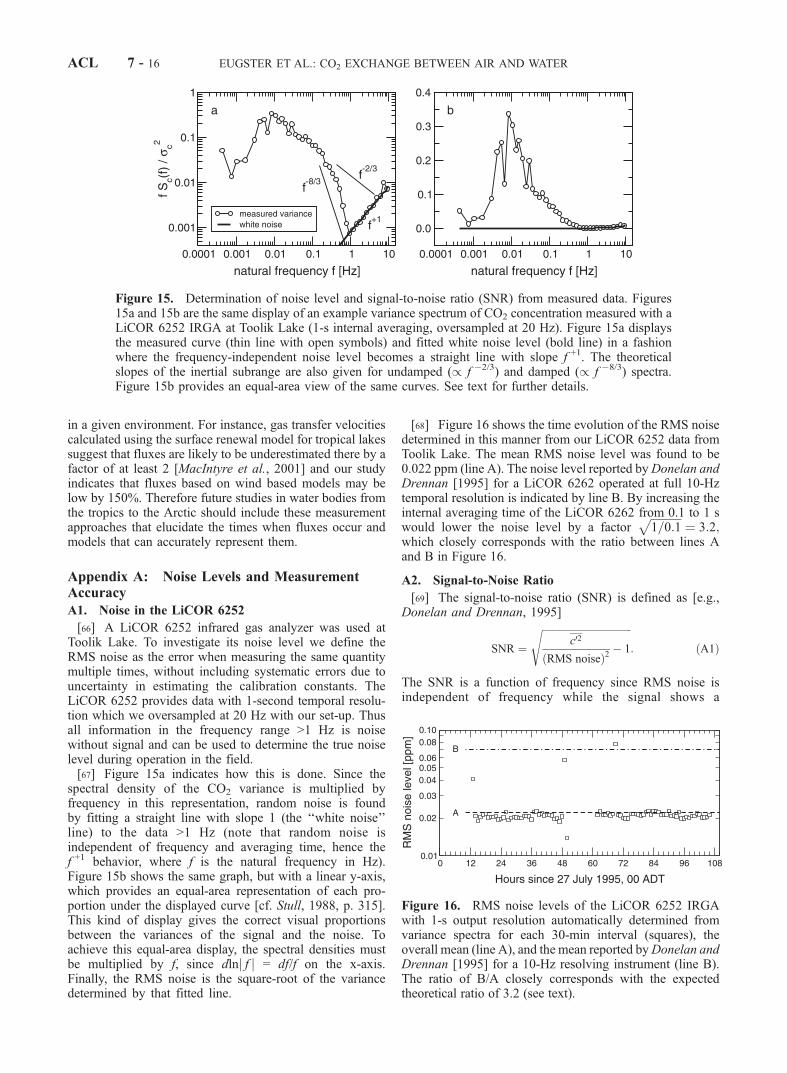
[66] A LiCOR 6252 infrared gas analyzer was used atToolik Lake. To investigate its noise level we define theRMS noise as the error when measuring the same quantitymultiple times, without including systematic errors due touncertainty in estimating the calibration constants. TheLiCOR 6252 provides data with 1-second temporal resolu-tion which we oversampled at 20 Hz with our set-up. Thusall information in the frequency range >1 Hz is noisewithout signal and can be used to determine the true noiselevel during operation in the field.[67] Figure 15a indicates how this is done. Since the

spectral density of the CO2 variance is multiplied byfrequency in this representation, random noise is foundby fitting a straight line with slope 1 (the ‘‘white noise’’line) to the data >1 Hz (note that random noise isindependent of frequency and averaging time, hence thef +1 behavior, where f is the natural frequency in Hz).Figure 15b shows the same graph, but with a linear y-axis,which provides an equal-area representation of each pro-portion under the displayed curve [cf. Stull, 1988, p. 315].This kind of display gives the correct visual proportionsbetween the variances of the signal and the noise. Toachieve this equal-area display, the spectral densities mustbe multiplied by f, since dlnj f j = df/f on the x-axis.Finally, the RMS noise is the square-root of the variancedetermined by that fitted line.

[68] Figure 16 shows the time evolution of the RMS noisedetermined in this manner from our LiCOR 6252 data fromToolik Lake. The mean RMS noise level was found to be0.022 ppm (line A). The noise level reported byDonelan andDrennan [1995] for a LiCOR 6262 operated at full 10-Hztemporal resolution is indicated by line B. By increasing theinternal averaging time of the LiCOR 6262 from 0.1 to 1 swould lower the noise level by a factor

ffiffiffiffiffiffiffiffiffiffiffi1=0:1

p¼ 3:2;

which closely corresponds with the ratio between lines Aand B in Figure 16.

A2. Signal-to-Noise Ratio

[69] The signal-to-noise ratio (SNR) is defined as [e.g.,Donelan and Drennan, 1995]

SNR ¼

ffiffiffiffiffiffiffiffiffiffiffiffiffiffiffiffiffiffiffiffiffiffiffiffiffiffiffiffiffiffiffiffiffiffiffiffic02

RMS noiseð Þ2� 1

s: ðA1Þ

The SNR is a function of frequency since RMS noise isindependent of frequency while the signal shows a

Figure 15. Determination of noise level and signal-to-noise ratio (SNR) from measured data. Figures15a and 15b are the same display of an example variance spectrum of CO2 concentration measured with aLiCOR 6252 IRGA at Toolik Lake (1-s internal averaging, oversampled at 20 Hz). Figure 15a displaysthe measured curve (thin line with open symbols) and fitted white noise level (bold line) in a fashionwhere the frequency-independent noise level becomes a straight line with slope f +1. The theoreticalslopes of the inertial subrange are also given for undamped (/ f �2/3) and damped (/ f �8/3) spectra.Figure 15b provides an equal-area view of the same curves. See text for further details.

Figure 16. RMS noise levels of the LiCOR 6252 IRGAwith 1-s output resolution automatically determined fromvariance spectra for each 30-min interval (squares), theoverall mean (line A), and the mean reported byDonelan andDrennan [1995] for a 10-Hz resolving instrument (line B).The ratio of B/A closely corresponds with the expectedtheoretical ratio of 3.2 (see text).


characteristic frequency spectrum. Equation (A1) cantherefore be clarified by writing

SNR fð Þ ¼

ffiffiffiffiffiffiffiffiffiffiffiffiffiffiffiffiffiffiffiffiffiffiffiffiffiffiffiffiffiffiffiffiffiffiffifficð f Þ02

RMS noiseð Þ2� 1

vuut ðA2Þ

for the SNR observed at a specific frequency.[70] In Figure 15, for example, the SNR( f > 1 Hz) = 0,

since the LiCOR 6252 has an output resolution of 1 Hz. Foreddy covariance flux measurements, however, a low SNR athigh frequency is not a concern, since the SNR tends to getvery large toward the low frequencies. When averaging over5 or 30 min (or even longer periods), the signal used for thevariance and covariance computations is taken from allfrequencies above the truncation frequency determined bythe length of the averaging period. Thus, in this paper, wereport the SNR as the average of f > 0.0033 Hz, which isthe truncation frequency of a 5-min averaging period.

A3. Accuracy of Flux Measurements

[71] The covariance w0c0 is related to the variances of thevertical wind speed sw

2 and of the CO2 fluctuations sc2 via

the correlation coefficient rw,c [e.g., Wilks, 1995, p. 46],

rw;c ¼w0c0

sw � sc: ðA3Þ

[72] Under the assumption that noise is random, and thatnoise in w is not correlated with noise observed in c (thatis, rw,c = 0), then the covariance should be zero no matterhow high the noise level in either signal is. In reality, thisis not perfectly the case, and thus we performed anexperiment by putting our sonic anemometer sensor headtogether with the NOAA IRGA into a cardboard box thatwas coated with plastic bubble wrap to minimize acousticreflections inside the box. The box was then loosely sealedwith tape in order to allow for heat and CO2 exchangewith the laboratory.[73] Data were collected at 20 Hz sampling rate during

20 hours and then processed as 30-min and 5-min aver-ages. The last 9 hours (nighttime, undisturbed) were usedto estimate the minimum repeatable CO2 flux measure-ment, and the first 7 hours (daytime, with disturbances)were used to analyze the potential effects of quick changesin CO2 concentration inside the box on the computedcovariances.A3.1. Minimum Repeatable CO2 Flux Measurement[74] The CO2 concentration in the box was 461 ppm

(laboratory background concentration), dropping from477 ppm after the last person had left to 448 ppm beforethe first person arrived the next morning. The root-mean-square standard deviation of the CO2 flux measurementswere between 0.197 and 0.292 ppm with an average of0.219 ppm for the 5-min averaging interval, and 0.202–0.800 ppm (average 0.443 ppm) for the 30-min averaginginterval, thus indicating that the trend in concentration has alarger influence with the longer averaging time. Neverthe-less, the arbitrary CO2 fluxes ranged between �1.26 � 10�4

and 4.6 � 10�5 mg C m�2 s�1, and between �3.9 � 10�5 and2.2 � 10�5 mg C m�2 s�1 when averaged over 5 and 30 min

intervals, respectively. This is at least two orders of magni-tude better than what would be needed to resolve the fluxesreported in our paper. Thus, despite the clearly higher noiselevel of the NOAA IRGA used at Soppensee, the accuracyof the flux measurements does not seem to be seriouslyaffected by noise. However, the large density flux correc-tions according to Webb et al. [1980] remain a concern foraccurate EC flux measurements over water surfaces.[75] The RMS standard deviations of the wind vector

components were largest for the vertical component. Ourmeasurements were between 0.008 and 0.015 m s�1, andthe correlation coefficient between the noise in c and theone in w (equation (A3)) was between �0.111 and 0.052 forthe 5-min averaging intervals. When averaging was doneover 30 min, all variances and correlations got closer to zeroroughly by the same factor as the length of the averagingperiod increased. If noise in w and c were of the samesource and thus rw,c = 1, the apparent flux computed withequation (A3) would still only be 0.002 mg C m�2 s�1 atworst.[76] Our minimum repeatable CO2 flux measurement

derived in this laboratory experiment under controlled andundisturbed conditions was better than 1.3 � 10�4 and 3.9 �10�5 mg C m�2 s�1 for 5 and 30 min averaging times,respectively.A3.2. Effect of Disturbance on the CO2

Flux Measurement[77] To simulate the effect of advection of high concen-

trations of CO2 from the land to the lake we allowedpeople access to the laboratory where we carried out ourzero flux experiment. The CO2 concentration thus variedbetween 450 and 560 ppm during the first 7 hours of theexperiment. The steepest increase observed was 102 ppmwithin 30 min. The largest (absolute magnitude) of appar-ent CO2 flux measured inside our box was 0.001 and0.005 mg C m�2 s�1 for the 5 and 30 min averages,respectively. Although the change in CO2 concentration inthis simulation was much larger than what was observedover Soppensee, the apparent fluxes are at least one orderof magnitude smaller than the peaks in our measurementsduring convective conditions. Moreover, this experimentclearly demonstrates the expected effect that 5-min aver-ages are less sensitive to such erratic occurrences (oradvection) than 30-min averages.[78] This is not to say that advection is not a relevant

issue. It is to be interpreted in the way that advection is arelevant source for the high CO2 concentration over ourlakes observed at night, but the eddy covariance method,since it is a method to measure turbulent, not advectivefluxes, is quite robust against such effects.

[79] Acknowledgments. The Toolik Lake measurements were per-formed as a part of the Arctic System Science Flux Study funded by U.S.National Science Foundation grants OPP-9318532 (F.S.C.), 9318529, and9615949 (G.K.). Measurements at Soppensee were funded by the SwissNational Science Foundation, grants 20-50761.97 and 2000-063723.00.W.E. was funded by a Hans Sigrist Fellowship grant of the University ofBern for analyzing the data and publishing the results. S.M. was supportedby NSF grants DEB9726930 and DEB0108572. We thank William S.Reeburgh for the loan of the LI-COR 6252 instrument during the 1995experiment and Rolf Siegwolf and Peter Geissbuhler, PSI, for the loan of aLI-COR 6262 instrumental setup used for gradient measurements atSoppensee. Gilda Gamarra, Ian Moore, Bryan Harper, Tom Ravens, andMichael Schurter provided support in the field. Lorenz Moosmann assisted


with data analysis. William Drennan, University of Miami, kindly helped toclarify the issue on signal-to-noise ratios, and three anonymous reviewershelped to improve the manuscript.

ReferencesAnderson, D. E., R. G. Striegl, D. I. Stannard, C. M. Michmerhuizen, T. A.McConnaughey, and J. W. LaBaugh, Estimating lake-atmosphere CO2

exchange, Limnol. Oceanogr., 44, 988–1001, 1999.Arya, S. P. S., Introduction to Micrometeorology, 307 pp., Academic Press,San Diego, 1988.

Auble, D. L., and T. P. Meyers, An open path, fast response infraredabsorption gas analyzer for H2O and CO2, Boundary Layer Meteorol.,59, 243–256, 1992.

Baldocchi, D., A comparative study of mass and energy exchange ratesover a closed C3 (wheat) and an open C4 (corn) crop: II. CO2 exchangeand water use efficiency, Agric. For. Meteorol., 67, 291–321, 1994.

Belanger, T. V., and E. A. Korzun, Critique of the floating-dome techniquefor estimating reaeration rates, J. Environ. Eng., 117, 144–150, 1990.

Cole, J. J., and N. F. Caraco, Atmospheric exchange of carbon dioxide in alow-wind oligotrophic lake measured by the addition of SF6, Limnol.Oceanogr., 43, 647–656, 1998.

Cole, J. J., N. F. Caraco, G. W. Kling, and T. K. Kratz, Carbon dioxidesupersaturation in the surface waters of lakes, Science, 265, 1568–1570,1994.

Crill, P., K. B. Bartlett, J. D. Wilson, D. K. Sebacker, R. C. Harriss, J. M.Melack, S. MacIntyre, L. Lesack, and L. Smith-Morrill, Trophosphericmethane from an Amazon floodplain lake, J. Geophys. Res., 93, 1564–1570, 1988.

Deardorff, J. W., Convective velocity and temperature scales for unstableplanetary boundary layer and for Rayleigh convection, J. Atmos. Sci., 27,1211–1213, 1970.

Donelan, M. A., and W. M. Drennan, Direct field measurements of theflux of carbon dioxide, in Air-Water Gas Transfer, edited by B. Jahne andE. C. Monahan, pp. 677–683, Aeon-Verlag, Heidelberg, Germany, 1995.

Edwards, G. C., H. H. Neumann, G. den Hartog, G. W. Thurtell, and G. E.Kidd, Eddy correlation measurements of methane fluxes using a tunablediode laser at the Kinosheo Lake tower site during the Northern WetlandsStudy (NOWES), J. Geophys. Res., 99, 1511–1517, 1994.

Eugster, W., and W. Senn, A cospectral correction model for measurementof turbulent NO2 flux, Boundary Layer Meteorol., 74, 321–340, 1995.

Fairall, C. W., J. E. Hare, J. B. Edson, and W. McGillis, Parameterizationand micrometeorological measurement of air-sea gas transfer, BoundaryLayer Meteorol., 96, 63–105, 2000.

Field, R. T., L. J. Fritschen, E. T. Kanemasu, E. A. Smith, J. B. Stewart,S. B. Verma, and W. P. Kustas, Calibration, comparison, and correction ofnet radiation instruments used during FIFE, J. Geophys. Res., 97,18,681–18,695, 1992.

Francey, R. J., and J. R. Garratt, Eddy flux measurements over the oceanand related transfer coefficients, Boundary Layer Meteorol., 14, 153–166, 1978.

Fritschen, L. J., Construction and calibration details of the thermal-transdu-cer-type net radiometer, Bull. Am. Meteorol. Soc., 41, 180–183, 1960.

Gruber, N., B. Wehrli, and A. Wuest, The role of biogeochemical cyclingfor the formation and preservation of varved sediments in Soppensee,J. Paleolimnol., 24, 277–291, 2000.

Horst, T. W., On frequency response corrections for eddy covariance fluxmeasurements, Boundary Layer Meteorol., 94, 517–520, 2000.

Imberger, J., The diurnal mixed layer, Limnol. Oceanogr., 30, 737–770,1985.

Jonas, T., A. Wuest, A. Stips, and W. Eugster, Observations of a quasi-shear-free convective boundary layer: Stratification and its implicationson turbulence, J. Geophys. Res., 108, doi:10.1029/2002JC001440, inpress, 2003.

Jones, E. P., and S. D. Smith, A first measurement of sea-air CO2 flux byeddy correlation, J. Geophys. Res., 82, 5990–5992, 1977.

Kaimal, J. C., and J. J. Finnigan, Atmospheric Boundary Layer Flows:Their Structure and Measurement, 289 pp., Oxford Univ. Press, NewYork, 1994.

Kaimal, J. C., J. C. Wyngaard, Y. Izumi, and O. R. Cote, Spectral char-acteristics of surface-layer turbulence, Q. J. R. Meteorol. Soc., 98, 563–589, 1972.

Kling, G. W., G. W. Kipphut, and M. C. Miller, Arctic lakes and streams asgas conduits to the atmosphere: Implications for tundra carbon budgets,Science, 251, 298–301, 1991.

Kling, G. W., G. W. Kipphut, and M. C. Miller, The flux of carbon dioxideand methane from lakes and rivers in arctic Alaska, Hydrobiologia, 240,23–36, 1992.

Kling, G. W., G. W. Kipphut, M. C. Miller, and W. J. O’Brien, Integrationof lakes and streams in a landscape perspective: The importance of

material processing on spatial patterns and temporal coherence, Fresh-water Biol., 43, 477–497, 2000.

Kocsis, O., H. Prandke, A. Stips, A. Simon, and A. Wuest, Comparison ofdissipation of turbulent kinetic energy determined from shear and tem-perature microstructure, J. Mar. Syst., 21, 67–84, 1999.

Lenschow, D. H., Micrometeorological techniques for measuring bio-sphere-atmosphere trace gas exchange, in Biogenic Trace Gases: Mea-suring Emissions From Soil and Water, Methods Ecol., edited by P. A.Matson and R. C. Harriss, pp. 126–163, Blackwell Sci., Malden, Mass.,1995.

Leuning, R., and M. J. Judd, The relative merits of open- and closed-pathanalysers for measurement of eddy fluxes, Global Change Biol., 2, 241–253, 1996.

Leuning, R., and K. M. King, Comparison of eddy-covariance measure-ments of CO2 flux by open- and closed-path CO2 analysers, BoundaryLayer Meteorol., 59, 297–311, 1992.

Leuning, R., and J. Moncrieff, Eddy-covariance CO2 flux measurementsusing open- and closed-path CO2 analysers: Corrections for analyserwater vapour sensitivity and damping of fluctuations in air samplingtubes, Boundary Layer Meteorol., 53, 63–76, 1990.

Leuning, R., O. T. Denmead, A. R. G. Lang, and E. Ohtaki, Effects of heatand water vapor transport on eddy covariance measurement of CO2

fluxes, Boundary Layer Meteorol., 23, 209–222, 1982.Livingston, G. P., and G. L. Hutchinson, Enclosure-based measurement oftrace gas exchange: Applications and sources of error, in Biogenic TraceGases: Measuring Emissions From Soil and Water, Methods Ecol., editedby P. A. Matson and R. C. Harriss, pp. 14–51, Blackwell Sci., Malden,Mass., 1995.

Lotter, A. F., Evidence of annual layering in Holocene sediments of Sop-pensee, Switzerland, Aquat. Sci., 51, 19–30, 1989.

MacIntyre, S., R. Wanninkhof, and J. P. Chanton, Trace gas exchangeacross the air-water interface in freshwater and coastal marine environ-ments, in Biogenic Trace Gases: Measuring Emissions From Soil andWater, Methods Ecol., edited by P. A. Matson and R. C. Harriss, pp. 52–97, Blackwell Sci., Malden, Mass., 1995.

MacIntyre, S., K. M. Flynn, R. Jellison, and J. R. Romero, Boundarymixing and nutrient fluxes in Mono Lake, California, Limnol. Oceanogr.,44, 512–529, 1999.

MacIntyre, S., W. Eugster, and G. W. Kling, The critical importance ofbuoyancy flux for gas flux across the air-water interface, in Gas Transferat Water Surfaces, Geophys. Monogr. Ser., vol. 127, edited by M. A.Donelan et al., pp. 135–139, AGU, Washington, D.C., 2001.

MacIntyre, S., J. R. Romero, and G. W. Kling, Spatial-temporal variabilityin mixed layer deepening and lateral advection in an embayment of LakeVictoria, East Africa, Limnol. Oceanogr., 47, 656–671, 2002.

Massman, W. J., A simple method for estimating frequency response cor-rections for eddy covariance systems, Agric. For. Meteorol., 104, 185–198, 2000.

Massman, W. J., and X. Lee, Eddy covariance flux corrections and uncer-tainties in long-term studies of carbon and energy exchanges, Agric. For.Meteorol., 113, 121–144, 2002.

Matson, P. A., and R. C. Harriss (Eds.), Biogenic Trace Gases: MeasuringEmissions from Soil and Water, Methods Ecol., 394 pp., Blackwell Sci.,Malden, Mass., 1995.

McGillis, W. R., J. B. Edson, J. E. Hare, and C. W. Fairall, Direct covar-iance air-sea CO2 fluxes, J. Geophys. Res., 106, 16,729–16,745, 2001.

McMillen, R. T., An eddy correlation technique with extended applicabilityto non-simple terrain, Boundary Layer Meteorol., 43, 231–245, 1988.

O’Brien, W. J., et al., The limnology of Toolik Lake, in Freshwaters ofAlaska: Ecological Syntheses, Ecol. Ser., vol. 119, edited by A. M. Mil-ner and M. W. Oswood, pp. 61–106, Springer-Verlag, New York, 1997.

Ocampo-Torres, F. J., M. Donelan, N. Merzi, and F. Jia, Laboratory mea-surements of mass transfer of carbon dioxide and water vapour forsmooth and rough flow conditions, Tellus, Ser. B, 46, 16–32, 1994.

Ohmura, A., and K. Schroff, Physical characteristics of the Davos-typepyrradiometer for short- and long-wave radiation, Arch. Meteorol. Geo-phys. Bioklimatol., Ser. B, 33, 57–76, 1983.

Panofsky, H. A., and J. A. Dutton, Atmospheric Turbulence, 397 pp., JohnWiley, New York, 1984.

Rannik, U., and T. Vesala, Autoregressive filtering versus linear detrendingin estimation of fluxes by the eddy covariance method, Boundary LayerMeteorol., 91, 259–280, 1999.

Richey, J. E., J. M. Melack, A. K. Aufdenkampe, V. M. Ballester, and L. L.Hess, Outgassing from Amazonian rivers and wetlands as a large tropicalsource of atmospheric CO2, Nature, 416, 617–620, 2002.

Schladow, S. G., M. Lee, B. E Hrzeler, and P. B. Kelly, Oxygen transferacross the air-water interface by natural convection in lakes, Limnol.Oceanogr., 47, 1394–1404, 2002.

Schmid, H. P., Experimental design for flux measurements: Matching scalesof observations and fluxes, Agric. For. Meteorol., 87, 179–200, 1997.


Schmid, H. P., Footprint modeling for vegetation atmosphere exchangestudies: A review and perspective, Agric. For. Meteorol., 113, 159–183, 2002.

Schuepp, P. H., M. Y. Leclerc, J. I. MacPherson, and R. L. Desjardins,Footprint prediction of scalar fluxes from analytical solutions of thediffusion equation, Boundary Layer Meteorol., 50, 355–373, 1990.

Smith, S. D., and E. P. Jones, Evidence for wind-pumping of air-sea gasexchange based on direct measurements of CO2 fluxes, J. Geophys. Res.,90, 869–875, 1985.

Smith, S. D., and E. P. Jones, Isotopic and micrometeorological ocean CO2

fluxes: Different time and space scales, J. Geophys. Res., 91, 10,529–10,532, 1986.

Smith, S. D., R. J. Anderson, E. P. Jones, R. L. Desjardins, R. M. Moore,O. Hertzman, and B. D. Johnson, A new measurement of CO2 eddy fluxin the nearshore atmospheric surface layer, J. Geophys. Res., 96, 8881–8887, 1991.

Soloviev, A. V., and P. Schluessel, Parameterization of the temperaturedifference across the cool skin of the ocean and of the air-ocean gastransfer on the basis of modelling surface renewal, J. Phys. Oceanogr.,24, 1319–1332, 1994.

Soloviev, A. V., and P. Schluessel, A model of air-sea gas exchangeincorporating the physics of the turbulent boundary layer and the proper-ties of the sea surface, in Gas Transfer at Water Surfaces, Geophys.Monogr. Ser., vol. 127, edited by M. A. Donelan et al., pp. 141–146,AGU, Washington, D.C., 2001.

Soloviev, A. V., J. Edson, W. McGillis, P. Schluessel, and R. Wanninkof,Fine thermohaline structure and gas-exchange in the near-surface layer ofthe ocean during GasEx-98, in Gas Transfer at Water Surfaces, Geophys.Monogr. Ser., vol. 127, edited by M. A. Donelan et al., pp. 181–185,AGU, Washington, D.C., 2001.

Stephens, D. W., Preliminary evaluation of the floating dome method formeasuring reaeration rates, J. Res. U.S. Geol. Surv., 6, 547–552, 1978.

Stull, R. B., An Introduction to Boundary Layer Meteorology, 666 pp.,Kluwer Acad., Norwell, Mass., 1988.

Sun, J., R. Desjardins, L. Marth, and I. MacPherson, Transport of carbondioxide, water vapor, and ozone by turbulence and local circulations,J. Geophys. Res., 103, 25,873–25,885, 1998.

Sun, J., D. Vandemark, L. Mahrt, D. Vickers, T. Crawford, and C. Vogel,Momentum transfer over the coastal zone, J. Geophys. Res., 106,12,437–12,448, 2001.

Suyker, A. E., and S. B. Verma, Eddy correlation measurements of CO2

flux using a closed-path sensor: Theory and field tests against an open-path sensor, Boundary Layer Meteorol., 64, 391–407, 1996.

Wanninkhof, R., and W. M. McGillis, A cubic relationship between gastransfer and wind speed, Geophys. Res. Lett., 26, 1889–1893, 1999.

Webb, E. K., G. I. Pearman, and R. Leuning, Correction of flux measure-ments for density effects due to heat and water vapour transfer, Q. J. R.Meteorol. Soc., 106, 85–100, 1980.

Wesely, M. L., D. R. Cook, R. L. Hart, and R. M. Williams, Air-seaexchange of CO2 and evidence for enhanced upwelling fluxes, J. Geo-phys. Res., 87, 8827–8832, 1982.

Whiteman, C. D., K. J. Allwine, L. J. Fritschen, M. M. Orgill, and J. R.Simpson, Deep valley radiation and surface energy budget microclimates.Part I: Radiation, J. Appl. Meteorol., 28, 414–426, 1989.

Wilks, D. S., Statistical Methods in the Atmospheric Sciences, 467 pp.,Academic, San Diego, Calif., 1995.

Zeman, O., and N. O. Jensen, Modification of turbulence characteristics inflow over hills, Q. J. R. Meteorol. Soc., 113, 55–80, 1987.

��F. S. Chapin III, Institute of Arctic Biology, University of Alaska,

Fairbanks, AK 99775, USA.W. Eugster, Geographical Institute, University of Bern, Hallerstraße 12,

CH-3012 Bern, Switzerland. ([email protected])T. Jonas and A. Wuest, Swiss Federal Institute for Environmental Science

and Technology, Mail Box 611, CH-8600 Dubendorf, Switzerland.G. Kling, Department of Ecology and Evolutionary Biology, University

of Michigan, 830 North University Avenue, Ann Arbor, MI 48109-1048,USA.S. MacIntyre, Marine Science Institute and Institute for Computational

Earth System Science, University of California, 6838 Ellison Hall, SantaBarbara, CA 93106, USA.J. P. McFadden, Department of Ecology, Evolution, and Behavior,

University of Minnesota, St. Paul, MN 55108, USA.


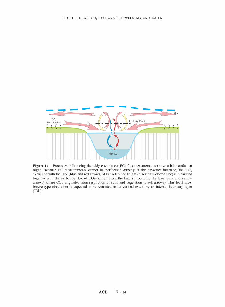
Figure 14. Processes influencing the eddy covariance (EC) flux measurements above a lake surface atnight. Because EC measurements cannot be performed directly at the air-water interface, the CO2

exchange with the lake (blue and red arrows) at EC reference height (black dash-dotted line) is measuredtogether with the exchange flux of CO2-rich air from the land surrounding the lake (pink and yellowarrows) where CO2 originates from respiration of soils and vegetation (black arrows). This local lake-breeze type circulation is expected to be restricted in its vertical extent by an internal boundary layer(IBL).

EUGSTER ET AL.: CO2 EXCHANGE BETWEEN AIR AND WATER

ACL 7 - 14

co exchange between air and water in an arctic alaskan and...

Documents