cmpsci 187 1 computer science 187 introduction to introduction to programming with data structures...

1

CMPSCI 187CMPSCI 187

Computer Science 187Computer Science 187Computer Science 187Computer Science 187

Introduction to Introduction to Programming with Data Structures

Introduction to Introduction to Programming with Data Structures

Lecture 25Lecture 25Graphs - Part 2Graphs - Part 2

Lecture 25Lecture 25Graphs - Part 2Graphs - Part 2

AnnouncementsAnnouncements

2


Directed Graphs: digraphsDirected Graphs: digraphs

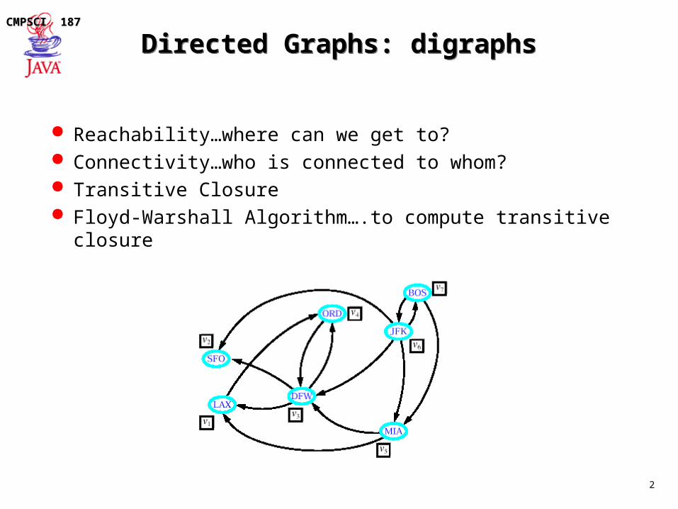
Reachability…where can we get to? Connectivity…who is connected to whom? Transitive Closure Floyd-Warshall Algorithm….to compute transitive closure

3


DigraphsDigraphs

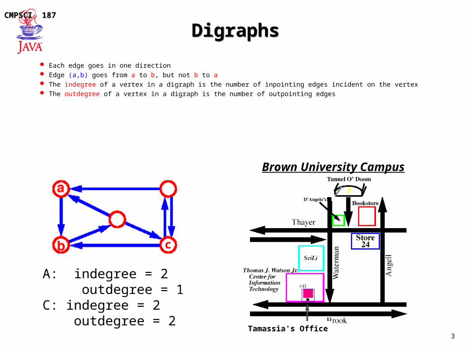
Each edge goes in one direction Edge (a,b) goes from a to b, but not b to a The indegree of a vertex in a digraph is the number of inpointing edges incident on the vertex The outdegree of a vertex in a digraph is the number of outpointing edges

Tamassia's Office

Brown University Campus

A: indegree = 2 outdegree = 1C: indegree = 2 outdegree = 2

c

4


Another Application: SchedulingAnother Application: Scheduling

Scheduling: edge (a,b) means task a must be completed before b can be started

5


Directed Acyclic Graphs: dagsDirected Acyclic Graphs: dags

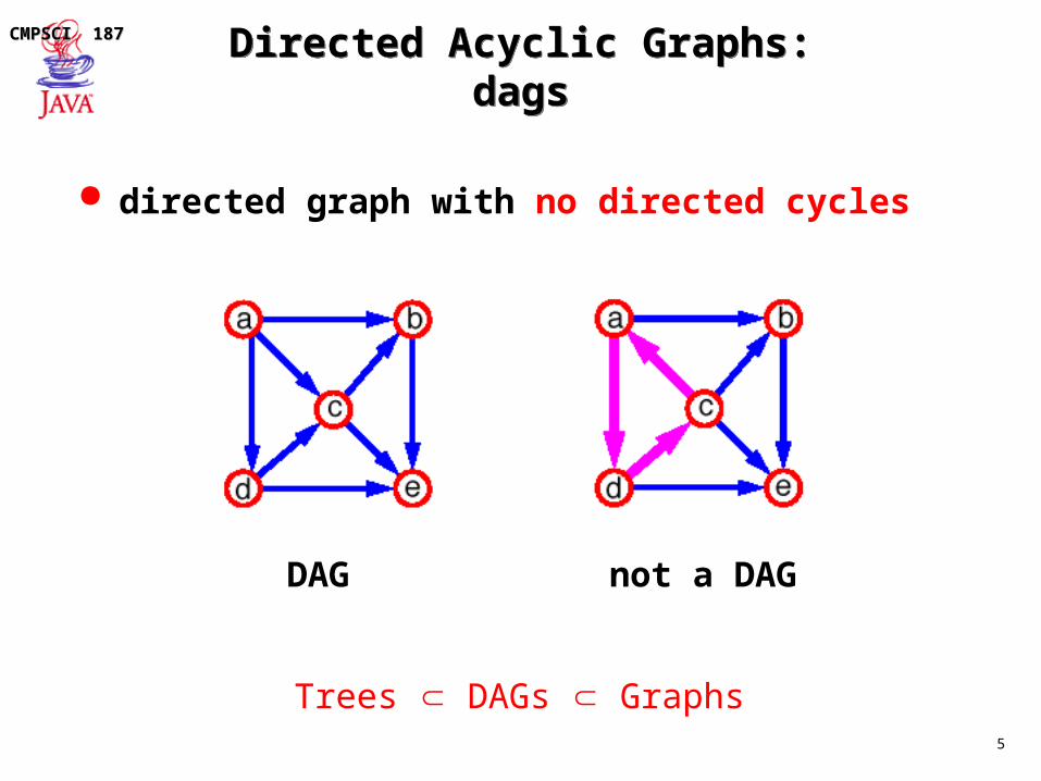
directed graph with no directed cycles

DAG not a DAG

Trees DAGs Graphs

6


Simple Paths and CyclesSimple Paths and Cycles

A simple path repeats no vertices (except that the first can be the last): p = {Seattle, Salt Lake City, San Francisco, Dallas} p = {Seattle, Salt Lake City, Dallas, San Francisco, Seattle}

A cycle is a path that starts and ends at the same vertex: p = {Seattle, Salt Lake City, Dallas, San Francisco, Seattle} p = {Chicago, Dallas, Salt Lake, Chicago, Dallas, Chicago

A simple cycle is a cycle that repeats no vertices except that the first vertex is also the last (in undirected graphs, no edge can be repeated) p = {Seattle, Salt Lake City, Dallas, San Francisco, Seattle}

Seattle

San Francisco

ChicagoSalt Lake City

Dallas

7


Depth First SearchDepth First Search

Same algorithm as for undirected graphs On a connected digraph, may yield unconnected DFS

trees (i.e., a DFS forest)

8


ReachabilityReachability

DFS tree rooted at v: vertices reachable from v via directed paths

Interesting problems dealing with reachability in a digraph G: Given vertices u and v, determine whether u reaches v. Find all vertices of G that are reachable from a given vertex s. Determine whether G is strong connected. Determine whether G is acyclic Compute the transitive closure G* of G.

9


Reachability ExamplesReachability Examples

A directed path from BOS to LAX is shown in red.

Bos

JFK

MIADFW

ORD

SFO

LAX

Bos

JFK

MIADFW

ORD

SFO

LAX

A directed cycle (ORD, MIA, DFW, LAX, ORD) is shown in red; its vertices induce a strongly connected subgraph

Bos

JFK

MIADFW

ORD

SFO

LAX

The subgraph of vertices and edges reachable from ORD is shown in red.

Bos

JFK

MIADFW

ORD

SFO

LAX

Removing the dashed red lines results in a directed acyclic graph.

10


Strongly Connected DigraphStrongly Connected Digraph

Each vertex can reach all other vertices

11


Strongly Connected ComponentsStrongly Connected Components

{ a , c , g }{ f , d , e , b }

12


Transitive ClosureTransitive Closure

Digraph G * is obtained from G using the rule: If there is a directed path in G from a to b, then add the

edge (a,b) to G *

G* is called the transitive closure of G.

G G*

Added

13


DefinitionsDefinitions

Undirected graphs are connected if there is a path between any two vertices

Directed graphs are strongly connected if there is a path from any one vertex to any other

Di-graphs are weakly connected if there is a path between any two vertices, ignoring direction

A complete graph has an edge between every pair of vertices

14


DFS and BFS for DigraphsDFS and BFS for Digraphs

Algorithms are very similar to their undirected counterparts. Algorithms only traverse edges according to their respective directions.

Searches can be used to answer reachability questions DFS on G starting at vertex s visits all the vertices of G that are reachable from s. The DFS tree contains directed paths from s to every vertex reachable from s.

If G is a digraph with n vertices and m edges, then DFS runs in O(n+m). The following problems can be solved by an algorithm that traverse G n times using

DFS; complexities are O(n(n+m)): Computing, for each vertex of G, the subgraph reachable from v Testing whether G is strongly connected Computing the transitive closure G* of G

15


Topological SortTopological Sort

Given a graph, G = (V, E), output all the vertices in V such that no vertex is output before any other vertex with an edge to it.

check inairport

calltaxi

taxi toairport

reserveflight

packbags

takeflight

locategate

16


Topological Sort: General IdeaTopological Sort: General Idea

Label each vertex’s in-degree (# of inbound edges)

While there are vertices remaining

Pick a vertex with in-degree of zero and output it

Reduce the in-degree of all vertices adjacent to it

Remove it from the list of vertices

17


Topological Sort RefinementTopological Sort Refinement

Label each vertex’s in-degree

Initialize a queue to contain all in-degree zero vertices

While there are vertices remaining in the queue

Pick a vertex v with in-degree of zero and output it

Reduce the in-degree of all vertices adjacent to v

Put any of these with new in-degree zero on the queue

Remove v from the queue

18


Weighted GraphsWeighted Graphs

Weighted Graphs weights on the edges of a graph represent distances, costs, etc. An example of an undirected weighted graph:

Shortest Paths

19


Single Source Shortest PathSingle Source Shortest Path

Given a graph G = (V, E) and a vertex s V, find the shortest path from s to every vertex in V

Many variations: directed vs. undirected weighted vs. unweighted cyclic vs. acyclic positive weights only vs. negative weights allowed multiple weight types to optimize

20


The Trouble with Negative Weighted Cycles

The Trouble with Negative Weighted Cycles

A B

C D

E

2 10

1-5

2

What’s the shortest path from A to E?(or to B, C, or D, for that matter)

21


Shortest PathShortest Path

BFS finds paths with the minimum number of edges from the start vertex

Hencs, BFS finds shortest paths assuming that each edge has the same weight

In many applications, e.g., transportation networks, the edges of a graph have different weights.

How can we find paths of minimum total weight? Example - Boston to Los Angeles:

22


Dijkstra's AlgorithmDijkstra's Algorithm

Dijkstra’s algorithm finds shortest paths from a start vertex v to all the other vertices in a graph with

undirected edges (works for directed edges w/minor mods)

nonnegative edge weights

The algorithm computes for each vertex u the distance of u from the start vertex v, that is, the weight of a shortest path between v and u.

The algorithm keeps track of the set of vertices for which the distance has been computed, called the cloud C

23


Dijkstra's Algorithm, cont.Dijkstra's Algorithm, cont.

Every vertex has a label D associated with it. For any vertex u, we can refer to its D label as D[u].

D[u] stores an approximation of the distance between v and u. The algorithm will update a D[u] value when it finds a shorter path from v to u.

When a vertex u is added to the cloud, its label D[u] is equal to the actual (final) distance between the starting vertex v and vertex u.

Initially, we set - D[v] = 0 ...the distance from v to itself is 0... - D[u] = for u v ...these will change...

24


Expanding the CloudExpanding the Cloud

Repeat until all vertices have been put in the cloud: let u be a vertex not in the cloud that has smallest label D[u]. (On

the first iteration, naturally the starting vertex will be chosen.) we add u to the cloud C we update the labels of the adjacent vertices of u as follows

for each vertex z adjacent to u do if z is not in the cloud C then if D[u] + weight(u,z) < D[z] then D[z] = D[u] + weight(u,z)

The above step is called a relaxation of edge (u,z)

v was put in the cloud first. Then this u. Then this u.

85

90

25


PseudoCodePseudoCode

We use a priority queue Q to store the vertices not in the cloud, where D[v] is the key of a vertex v in Q

Algorithm ShortestPath(G, v):Input: A weighted graph G and a distinguished vertex v of G.Output: A label D[u], for each vertex u of G, such that D[u] is the length of a shortest path from v to u in G.

initialize D[v] 0 and D[u] + for each vertex v ulet Q be a priority queue that contains all of the vertices of G using the D labels as keys.while Q do {pull u into the cloud C} u Q.removeMinElement() for each vertex z adjacent to u such that z is in Q do {perform the relaxation operation on edge (u, z) } if D[u] + w((u, z)) < D[z] then D[z] D[u] + w((u, z)) change the key value of z in Q to D[z]return the label D[u] of each vertex u.

26


ExampleExample

BOS BWI 0DFW JFK BWI184LAX MIA BWI 946ORD BWI 621PVD SFO

Parent Distance


Pull JFK into the cloud and continue

27


JFK is the nearestJFK is the nearest

BOS JFK 371BWI 0DFW JFK 1575JFK BWI184LAX MIA BWI 946ORD BWI 621PVD JFK 328SFO

Parent Distance


u

Was Was 621

Was

Was 946Pull PVD into the cloud and continue

28


Followed by PVDFollowed by PVD

BOS JFK 371BWI 0DFW JFK 1575 JFK BWI184LAX MIA BWI 946ORD BWI 621PVD JFK 328SFO

Parent Distance

u


Pull BOS into the cloud and continue

29


Boston is just a bit furtherBoston is just a bit further

BOS JFK 371BWI 0DFW JFK 1575JFK BWI184LAX MIA BWI 946ORD BWI 621PVD JFK 328SFO BOS 3075

Parent Distance


Was

u

Pull ORD into the cloud and continue

30


Chicago is nextChicago is next

BOS JFK 371BWI 0DFW ORD 1423JFK BWI184LAX MIA BWI 946ORD BWI 621PVD JFK 328SFO ORD 2467

Parent Distance

Both were adjusted this turn

u

Was 1575

Was 3075

Pull MIA into the cloud and continue

31


Now MiamiNow Miami

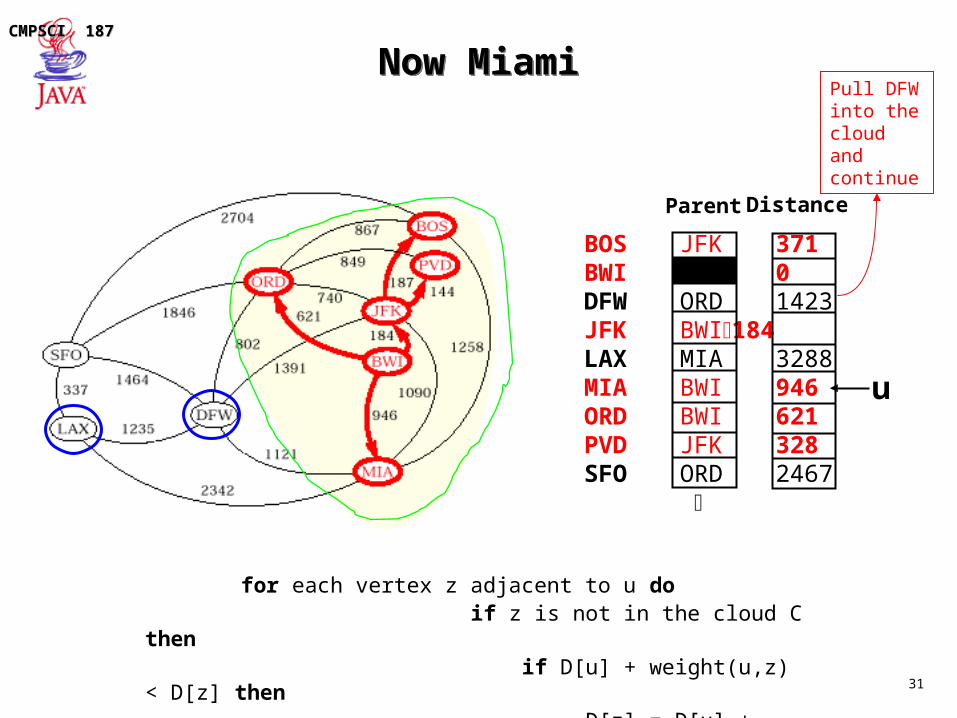
BOS JFK 371BWI 0DFW ORD 1423JFK BWI184LAX MIA 3288 MIA BWI 946ORD BWI 621PVD JFK 328SFO ORD 2467

Parent Distance

u


Pull DFW into the cloud and continue

32


Now Dallas-Fort WorthNow Dallas-Fort Worth

BOS JFK 371BWI 0DFW ORD 1423JFK BWI184LAX DFW 2658 MIA BWI 946ORD BWI 621PVD JFK 328SFO ORD 2467

Parent Distance

LAX was adjusted this turn

Pull SFO into the cloud and continue

u

33


Now San FranciscoNow San Francisco


Parent Distance

34


Finally, LAFinally, LA


Parent Distance

35


Running TimeRunning Time

Let’s assume that we represent G with an adjacency list. We can then step through all the vertices adjacent to u in time proportional to their number (i.e. O(deg u) where deg u in the number of vertices adjacent to u)

The priority queue Q - we have a choice: A Heap: Implementing Q with a heap allows for efficient extraction of vertices

with the smallest D label(O(logN)). Key updates can also be performed in O(logN) time. The total run time is O((n+m)logn) where n is the number of vertices in G and m in the number of edges. In terms of n, worst case time is O(n 2 logn)

An Unsorted Sequence: O(n) when we extract minimum elements, but fast key updates (O(1)). There are only n-1 extractions and m relaxations. The running time is O(n2 +m)

In terms of worst case time, heap is good for small data sets and sequence for larger.

36


Running Time, cont.Running Time, cont.

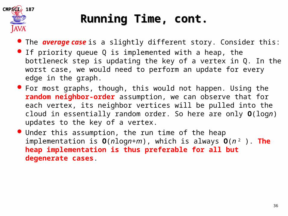
The average case is a slightly different story. Consider this: If priority queue Q is implemented with a heap, the bottleneck step

is updating the key of a vertex in Q. In the worst case, we would need to perform an update for every edge in the graph.

For most graphs, though, this would not happen. Using the random neighbor-order assumption, we can observe that for each vertex, its neighbor vertices will be pulled into the cloud in essentially random order. So here are only O(logn) updates to the key of a vertex.

Under this assumption, the run time of the heap implementation is O(nlogn+m), which is always O(n 2 ). The heap implementation is thus preferable for all but degenerate cases.

37


ObservationsObservations

In our example, the weight is the geographical distance. However, the weight could just as easily represent the cost or time to fly the given route.

We can easily modify Dijkstra’s algorithm for different needs, for instance: If we just want to know the shortest path from vertex v to a single

vertex u, we can stop the algorithm as soon as u is pulled into the cloud.

Or, we could have the algorithm output a tree T rooted at v such that the path in T from v to a vertex u is a shortest path from v to u.

38


Weighted GraphsWeighted Graphs

weight(G') = 800 + 400 + 1200

= 2400

(weight of subgraph G') = (sum of weights of edges of G')

weight(G') = weight(e)

(e G')

39


Minimum Spanning TreeMinimum Spanning Tree

spanning tree of minimum total weight e.g., connect all the computers in a building with the least amount

of cable Examples:

Minimum spanning trees are not generally unique

40


Applications of MSTsApplications of MSTs

Communication networks

VLSI design

Transportation systems

Good approximation to some NP-hard problems (take CS250)

41


Minimum Spanning Tree PropertyMinimum Spanning Tree Property

Let (V',V") be a partition of the vertices of G Let e = (v', v"), be an edge of minimum weight across

the partition,

i.e., v' V' and v" V". There is a MST containing edge e.

42


Proof of PropertyProof of Property

If the MST does not contain a minimum weight edge e, then we can find a better or equal MST by exchanging e for some other edge.

43


Prim-Jarnik Algorithm for the MSTPrim-Jarnik Algorithm for the MST

grows the MST T one vertex at a time cloud covering the portion of T already computed labels D[u] and E[u] associated with each vertex u

E[u] is the best (lowest weight) edge connecting u to T D[u] (distance to the cloud) is the weight of E[u]

44


Differences between Prim’s and Dijkstra’sDifferences between Prim’s and Dijkstra’s

For any vertex u, D[u] represents the weight of the current best edge for joining u to the rest of the tree (as opposed to the total sum of edge weights on a path from start vertex to u).

Use a priority queue Q whose keys are D labels, and whose elements are vertex-edge pairs.

Any vertex v can be the starting vertex. We still initialize all the D[u] values to INFINITE, but we

also initialize E[u] (the edge associated with u) to null. Return the minimum-spanning tree T.

We can reuse code from Dijkstra’s algorithm, and we only have to change a few things. Let’s look at the pseudocode....

45


Prim-Jarnik Pseudo CodePrim-Jarnik Pseudo Code

Algorithm PrimJarnik(G): Input: A weighted graph G. Output: A minimum spanning tree T for G.pick any vertex v of G {grow the tree starting with vertex v}T {v} D[u] 0 E[u] for each vertex u v do D[u] let Q be a priority queue that contains vertices, using the D labels as keyswhile Q do {pull u into the cloud C} uQ.removeMinElement() add vertex u and edge E[u] to T for each vertex z adjacent to u do if z is in Q {perform the relaxation operation on edge (u, z) } if weight(u, z) < D[z] then D[z] weight(u, z) E[z] (u, z) change the key of z in Q to D[z]return tree T

46


ExampleExample

DFW STL 400LAX STL 1800LGA STL 1200MIAMSN STL 800PVDSEASFOSTL

Neighbor D[u]

Start at v = STL

47


Closest is DFWClosest is DFW

DFW STL 400LAX DFW 1500LGA STL 1200MIA DFW 1000MSN STL 800PVDSEASFOSTL

Neighbor D[u]

D[u] updated when DFW added to cloud

48


Now Minneapolis-St. PaulNow Minneapolis-St. Paul

DFW STL 400LAX DFW 1500LGA MSN 1000MIA DFW 1000MSN STL 800PVDSEA MSN 1500SFOSTL

Neighbor D[u]

49


Now LaGuardiaNow LaGuardia

DFW STL 400LAX DFW 1500LGA MSN 1000MIA DFW 1000MSN STL 800PVD LGA 200SEA MSN 1500SFOSTL

Neighbor D[u]

50


Now ProvidenceNow Providence


Neighbor D[u]

PVD

200

51


Now MiamiNow Miami

PVD

200


Neighbor D[u]

MIA

1500

1000

52


Now SeattleNow Seattle

PVD

200

MIA

1500

DFW STL 400LAX DFW 1500LGA MSN 1000MIA DFW 1000MSN STL 800PVD LGA 200SEA MSN 1500SFO SEA 800STL

Neighbor D[u]

800

1500SEA

SFO

1000

53


Now SanFranciscoNow SanFrancisco

PVD

200

MIA

1500

800

1500SEA

SFO

DFW STL 400LAX SFO 400LGA MSN 1000MIA DFW 1000MSN STL 800PVD LGA 200SEA MSN 1500SFO SEA 800STL

Neighbor D[u]

400

1500

1000

54


Finally, Los AngelesFinally, Los Angeles

PVD

200

MIA

1500

800

1500SEA

SFO

400

1500

DFW STL 400LAX SFO 400LGA MSN 1000MIA DFW 1000MSN STL 800PVD LGA 200SEA MSN 1500SFO SEA 800STL

Neighbor D[u]

LAX

1000

55


Final Minimal Spanning TreeFinal Minimal Spanning Tree

STL

DFWMSN

SEALGAMIA

PVD SFO

LAX

800 400

800

400

15001000

200

1000

56


Running TimeRunning Time

Complexity O((n+m) log n)where n = num vertices, m=num edges, and Q is implemented with a heap.

57


Searching HUGE GraphsSearching HUGE Graphs

Consider some really huge graphs…All cities and towns in the World AtlasAll stars in the GalaxyAll ways 10 blocks can be stacked

Huh???

58


Implicitly Generated GraphsImplicitly Generated Graphs

A huge graph may be implicitly specified by rules for generating it on-the-fly

Blocks world: vertex = relative positions of all blocks edge = robot arm could stack one block

stack(blue,red)

stack(green,red)

stack(green,blue)

59


Robotics Blocks WorldRobotics Blocks World

Source = initial state of the blocks Goal = desired state of the blocks Path from source to goal = sequence of actions

(program) for robot arm!

n blocks nn states 10 blocks 10 billion states

stack(blue,red)

stack(green,blue)

Uh-Oh!

60

CMPSCI 187CMPSCI 187 Problem: Branching Factor or Out-degree of each vertex

Problem: Branching Factor or Out-degree of each vertex

Cannot search such huge graphs exhaustively. Suppose we know that goal is only d steps away.

Dijkstra’s algorithm is basically breadth-first search (taking into account the edge weights)

If the out-degree of each node is 10, potentially visits 10d vertices 10 step plan = 10 billion vertices!

61


A Simpler ExampleA Simpler Example

Suppose you live in Manhattan; what do you do?

52nd St

51st St

50th St

10th A

ve

9th A

ve

8th A

ve

7th A

ve

6th A

ve

5th A

ve

4th A

ve

3rd A

ve

2nd A

ve

S

G

62


Best-First SearchBest-First Search

The manhattan distance ( x+ y) is an estimate of the distance to the goal a heuristic value

Best-First Search Order nodes in priority to minimize estimated distance to the goal

Compare: Dijkstra Order nodes in priority to minimize distance from the start

52nd St

51st St

50th St 10th A

ve

9th A

ve

8th A

ve

7th A

ve

6th A

ve

5th A

ve

4th A

ve

3rd A

ve

2nd A

ve

SG

x

y

x= 6 y = 1Distance ~ 7

Best-First Action

63


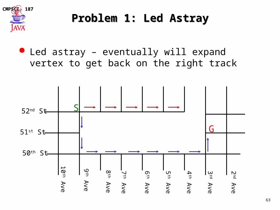
Problem 1: Led AstrayProblem 1: Led Astray

Led astray – eventually will expand vertex to get back on the right track

52nd St

51st St

50th St

10th A

ve

9th A

ve

8th A

ve

7th A

ve

6th A

ve

5th A

ve

4th A

ve

3rd A

ve

2nd A

ve

S

G

64


Problem 2: OptimalityProblem 2: Optimality

With Best-First Search, are you guaranteed a shortest path is found when goal is first seen? when goal is removed from priority queue?

No! Goal is by definition at distance 0: will be removed from priority queue immediately when it is seen, even if a shorter path exists!

52nd St

51st St

9th A

ve

8th A

ve

7th A

ve

6th A

ve

5th A

ve

4th A

ve

S

G

(5 blocks)Best-First Search typically results in a sub-optimal solution!

65


Dijkstra vs. Best-FirstDijkstra vs. Best-First

Dijkstra / Breadth First guaranteed to find optimal solution

Best First often visits far fewer vertices, but may not provide optimal solution

Can we get the best of both?

66


The A* AlgorithmThe A* Algorithm

Order vertices in priority queue to minimize (distance from start) + (estimated distance to goal)

f(n) = g(n) + h(n) Where:

f(n) = priority of a node

g(n) = true distance from start

h(n) = heuristic distance to goal

Suppose the estimated distance (h) is the true distance to the goal (heuristic is a lower bound)

Then: when the goal is removed from the priority queue, we are guaranteed to have found a shortest path!

67


Problem 2 RevisitedProblem 2 Revisited

52nd St

51st St

9th A

ve

8th A

ve

7th A

ve

6th A

ve

5th A

ve

4th A

veS

G

(5 blocks)

Priority = 1+4=5

Dijkstra would have

visited these guys!

50th St

Priority = 5+2=6

68


A Little HistoryA Little History

A* invented by Nils Nilsson & colleagues in 1968 or maybe some guy in Operations Research?

Cornerstone of artificial intelligence still a hot (OK - lukewarm) research topic! iterative deepening A*, automatically generating heuristic functions,

… Method of choice for search large (even infinite) graphs

when a good heuristic function can be found Proofs of optimality exist

69


Remember the Blocks?Remember the Blocks?

“Distance to goal” is not always physical distance Blocks world:

distance = number of stacks to perform heuristic lower bound = number of blocks out of place

# out of place = 2, true distance to goal = 3

1 2 3

70


Other ExamplesOther Examples

Simplifying Integrals vertex = formula goal = closed form formula without integrals arcs = mathematical transformations heuristic = number of integrals remaining in formula

Problem: given chopped up DNA, reassemble Vertex = set of pieces Arc = stick two pieces together Goal = only one piece left Heuristic = number of pieces remaining - 1

Lots More!

71


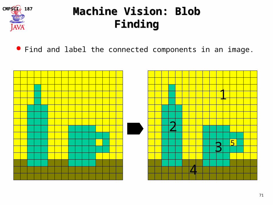
Machine Vision: Blob FindingMachine Vision: Blob Finding

Find and label the connected components in an image.

1

2

3

4

5

72


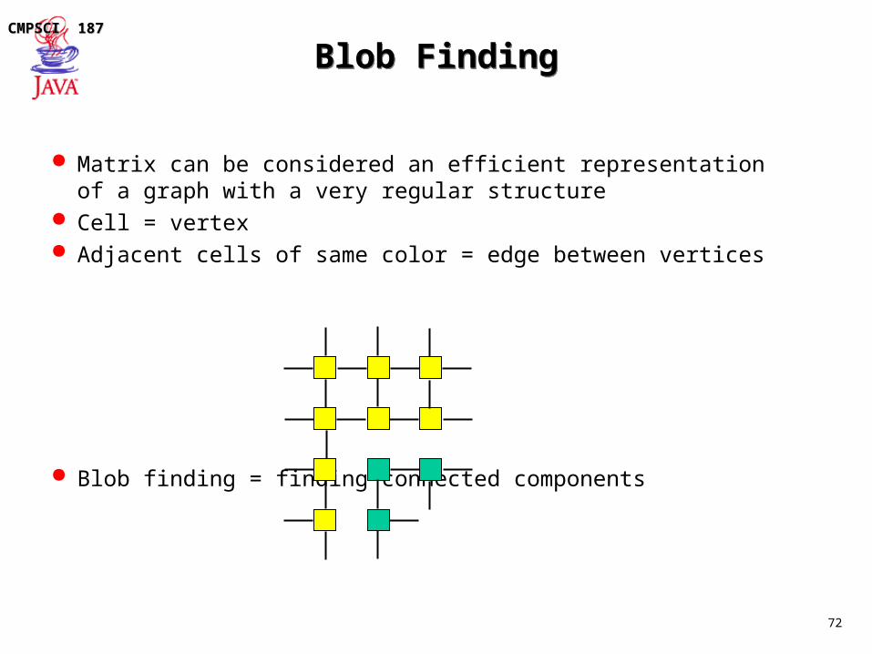
Blob FindingBlob Finding

Matrix can be considered an efficient representation of a graph with a very regular structure

Cell = vertex Adjacent cells of same color = edge between vertices

Blob finding = finding connected components

73


TradeoffsTradeoffs

DFS approache is (essentially) O(E+V) = O(V) for binary images Why?

For each component, DFS (“recursive labeling”) can move all over the image – entire image must be in main memory

Better in practice: row-by-row processing localizes accesses to memory

Algorithm: Scan through image left/right and top/bottom If a cell is same color as (connected to) cell to right or below, then

union them into an equivalence class {SET THEORETIC APPROACH} Give the same blob number to cells in each equivalence class

74


Blob Labeling AlgorithmBlob Labeling Algorithm

Put each cell <x,y> in its own equivalence classFor each cell <x,y>

if color[x,y] == color[x+1,y] thenUnion( <x,y>, <x+1,y> )

if color[x,y] == color[x,y+1] thenUnion( <x,y>, <x,y+1> )

label = 0For each root <x,y>

blobnum[x,y] = ++ label;For each cell <x,y>

blobnum[x,y] = blobnum( Find(<x,y>) )

75


cmpsci 187 1 computer science 187 introduction to introduction to programming with data structures...

Documents