1

CMPE 466COMPUTER GRAPHICSChapter 8

2D Viewing

Instructor: D. Arifler

Material based on- Computer Graphics with OpenGL®, Fourth Edition by Donald Hearn, M. Pauline Baker, and Warren R. Carithers- Fundamentals of Computer Graphics, Third Edition by by Peter Shirley and Steve Marschner- Computer Graphics by F. S. Hill

2

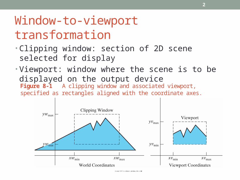
Window-to-viewport transformation

• Clipping window: section of 2D scene selected for display• Viewport: window where the scene is to be displayed on

the output device

Figure 8-1 A clipping window and associated viewport, specified as rectangles aligned with the coordinate axes.

3

Viewing pipeline

Figure 8-2 Two-dimensional viewing-transformation pipeline.

Normalization makes viewing device independentClipping can be applied to object descriptions in normalized coordinates

4

Viewing coordinates

Figure 8-3 A rotated clipping window defined in viewing coordinates.

5

Viewing coordinatesFigure 8-4 A viewing-coordinate frame is moved into coincidence with the world frame by (a) applying a translation matrix T to move the viewing origin to the world origin, then (b) applying a rotation matrix R to align the axes of the two systems.

6

View up vector

Figure 8-5 A triangle (a), with a selected reference point and orientation vector, is translated and rotated to position (b) within a clipping window.

7

Mapping the clipping window into normalized viewport

Figure 8-6 A point (xw, yw) in a world-coordinate clipping window is mapped to viewport coordinates (xv, yv), within a unit square, so that the relative positions of the two points in their respective rectangles are the same.

8

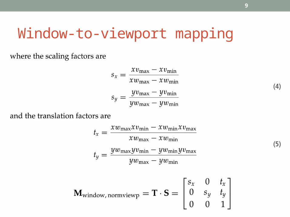
Window-to-viewport mapping

9

Window-to-viewport mapping

10

Alternative: mapping clipping window into a normalized square• Advantage: clipping algorithms are standardized (see

more later)• Substitute xvmin=yvmin=-1 and xvmax=yvmax=1

Figure 8-7 A point (xw, yw) in a clipping window is mapped to a normalized coordinate position (x norm, y norm), then to a screen-coordinate position (xv, yv) in a viewport. Objects are clipped against the normalization square before the transformation to viewport coordinates occurs.

11

Mapping to a normalized square

12

Finally, mapping to viewport

13

Screen, display window, viewport

Figure 8-8 A viewport at coordinate position (xs , ys ) within a display window.

14

OpenGL 2D viewing functions

• GLU clipping-window function

• OpenGL viewport function

15

Creating a GLUT display window

16

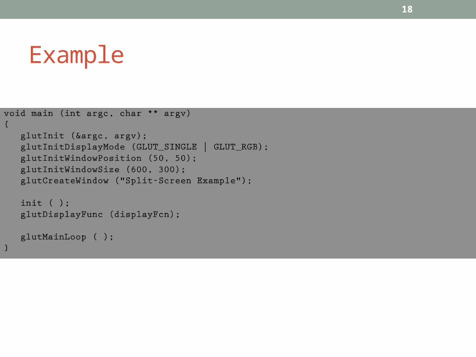
Example

17

Example

18

Example

19

2D point clipping

20

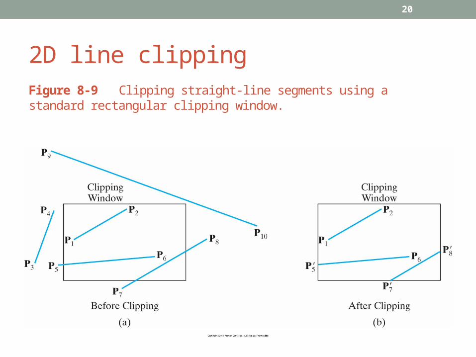
2D line clippingFigure 8-9 Clipping straight-line segments using a standard rectangular clipping window.

21

2D line clipping: basic approach

• Test if line is completely inside or outside• When both endpoints are inside all four clipping

boundaries, the line is completely inside the window• Testing of outside is more difficult: When both endpoints

are outside any one of four boundaries, line is completely outside

• If both tests fail, line segment intersects at least one clipping boundary and it may or may not cross into the interior of the clipping window

22

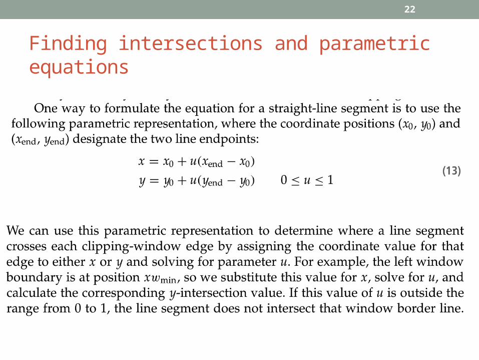
Finding intersections and parametric equations

23

Parametric equations and clipping

24

Cohen-Sutherland line clipping

• Perform more tests before finding intersections• Every line endpoint is assigned a 4-digit binary value

(region code or out code), and each bit position is used to indicate whether the point is inside or outside one of the clipping-window boundaries

• E.g., suppose that the coordinate of the endpoint is (x, y). Bit 1 is set to 1 if x<xwmin

25

Region codes

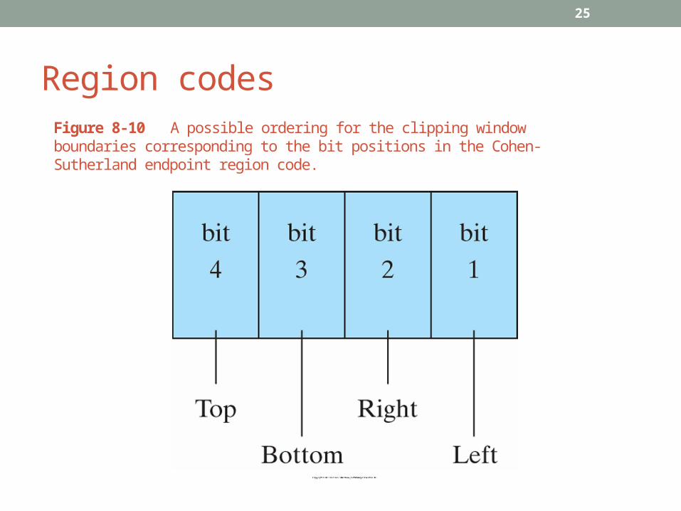
Figure 8-10 A possible ordering for the clipping window boundaries corresponding to the bit positions in the Cohen- Sutherland endpoint region code.

26

Region codesFigure 8-11 The nine binary region codes for identifying the position of a line endpoint, relative to the clipping-window boundaries.

27

Cohen-Sutherland line clipping: steps

• Calculate differences between endpoint coordinates and clipping boundaries

• Use the resultant sign bit of each difference to set the corresponding value in the region code• Bit 1 is the sign bit of x-xwmin

• Bit 2 is the sign bit of xwmax-x

• Bit 3 is the sign bit of y-ywmin

• Bit 4 is the sign bit of ywmax-y

• Any lines that are completely inside have a region code 0000 for both endpoints (save the line segment)

• Any line that has a region code value of 1 in the same bit position for each endpoint is completely outside (eliminate the line segment)

28

Cohen-Sutherland line clipping: inside-outside tests• For performance improvement, first do inside-outside

tests• When the OR operation between two endpoint region

codes for a line segment is FALSE (0000), the line is inside the clipping region

• When the AND operation between two endpoint region codes for a line is TRUE (not 0000), then line is completely outside the clipping window

• Lines that cannot be identified as being completely inside or completely outside are next checked for intersection with the window border lines

29

CS clipping: completely inside-outside?

Figure 8-12 Lines extending from one clipping-window region to another may cross into the clipping window, or they could intersect one or more clipping boundaries without entering the window.

30

CS clipping

• To determine whether the line crosses a selected clipping boundary, we check the corresponding bit values in the two endpoint region codes• If one of these bit values is 1 and the other is 0, the line segment

crosses that boundary

• To determine a boundary intersection for a line segment, we use the slope-intercept form of the line equation

• For a line with endpoint coordinates (x0, y0) and (xEnd, yEnd), the y coordinate of the intersection point with a vertical clipping border line can be obtained with the calculationy=y0+m(x-x0)

31

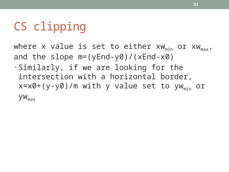
CS clipping

where x value is set to either xwmin or xwmax, and the slope m=(yEnd-y0)/(xEnd-x0)• Similarly, if we are looking for the intersection with a

horizontal border, x=x0+(y-y0)/m with y value set to ywmin or ywmax

32

Liang-Barsky line clipping

33

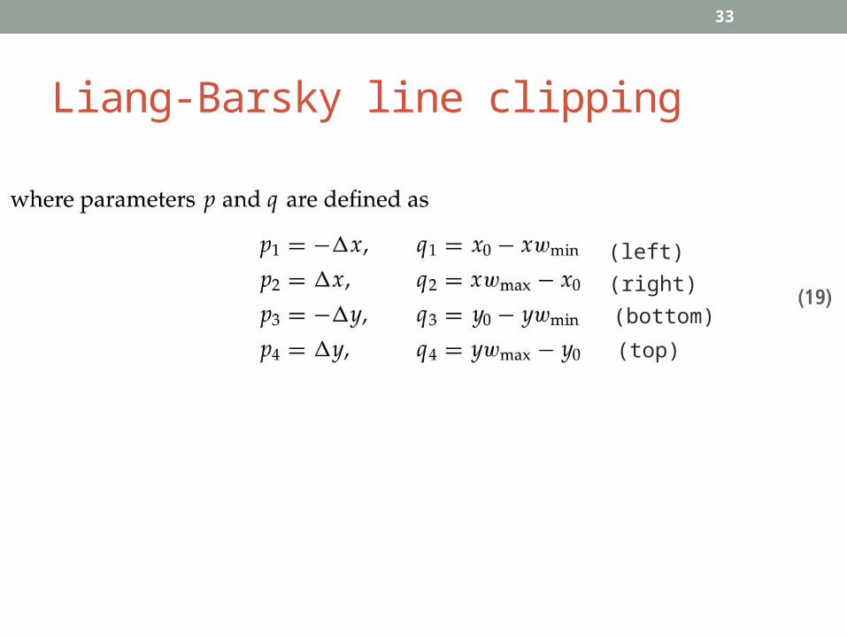
Liang-Barsky line clipping

(left)

(right)

(bottom)

(top)

34

Liang-Barsky line clipping

• If pk=0 (line parallel to clipping window edge)• If qk<0, the line is completely outside the boundary (clip)

• If qk≥0, the line is completely inside the parallel clipping border (needs further processing)

• When pk<0, infinite extension of line proceeds from outside to inside of the infinite extension of this particular clipping window edge

• When pk>0, line proceeds from inside to outside

• For non-zero pk, we can calculate the value of u that corresponds to the point where the infinitely extended line intersects the extension of the window edge k as u=qk/pk

35

LB algorithm

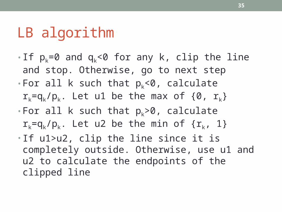
• If pk=0 and qk<0 for any k, clip the line and stop. Otherwise, go to next step

• For all k such that pk<0, calculate rk=qk/pk. Let u1 be the max of {0, rk}

• For all k such that pk>0, calculate rk=qk/pk. Let u2 be the min of {rk, 1}

• If u1>u2, clip the line since it is completely outside. Otherwise, use u1 and u2 to calculate the endpoints of the clipped line

36

Notes

• LB is more efficient than CS• Both CS and LB can be extended to 3D

37

Polygon Fill-Area Clipping

• Sutherland-Hodgman polygon clipping

Figure 8-24 The four possible outputs generated by the left clipper, depending on the position of a pair of endpoints relative to the left boundary of the clipping window.

38

Sutherland-Hodgman polygon clippingFigure 8-25 Processing a set of polygon vertices, {1, 2, 3}, through the boundary clippers using the Sutherland-Hodgman algorithm. The final set of clipped vertices is {1', 2, 2', 2''}.

39

Sutherland-Hodgman polygon clipping

• Send pair of endpoints for each successive polygon line segment through the series of clippers. Four possible cases:

1. If the first input vertex is outside this clipping-window border and the second vertex is inside, both the intersection point of the polygon edge with the window border and the second vertex are sent to the next clipper

2. If both input vertices are inside this clipping-window border, only the second vertex is sent to the next clipper

3. If the first vertex is inside and the second vertex is outside, only the polygon edge intersection position with the clipping-window border is sent to the next clipper

4. If both input vertices are outside this clipping-window border, no vertices are sent to the next clipper

40

Sutherland-Hodgman polygon clipping

• The last clipper in this series generates a vertex list that describes the final clipped fill area

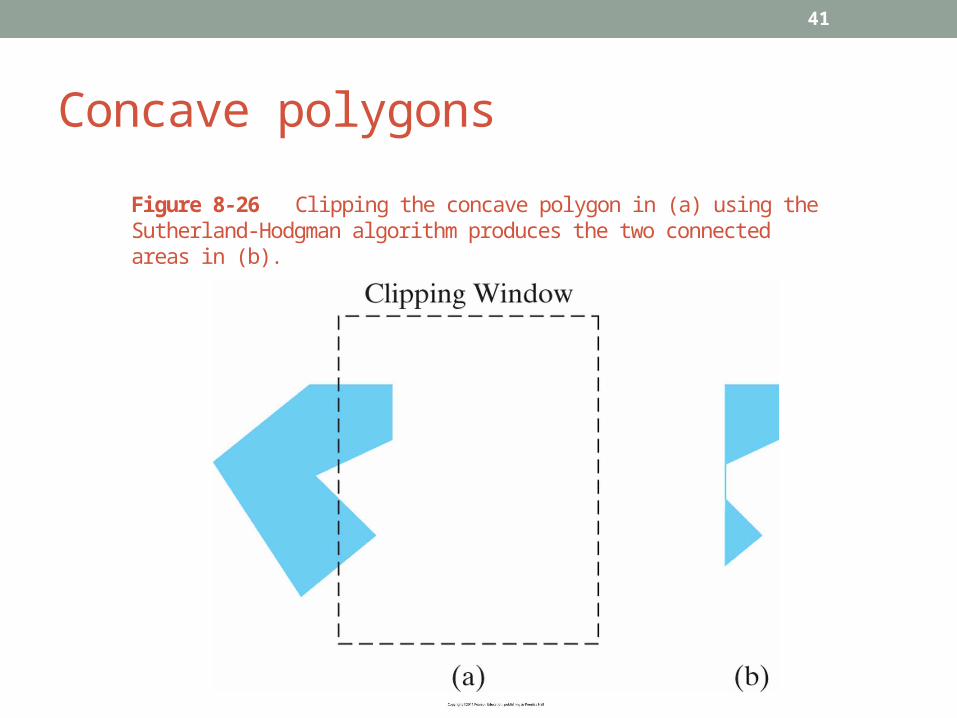
• When a concave polygon is clipped, extraneous lines may be displayed. Solution is to split a concave polygon into two or more convex polygons

41

Concave polygons

Figure 8-26 Clipping the concave polygon in (a) using the Sutherland-Hodgman algorithm produces the two connected areas in (b).