cmat2 / midas comparison · pdf filesystem which performs 3d tomography of the ionosphere....

© Crown copyright Met Office

CMAT2 / MIDAS comparison CEDAR 2014, Seattle. Presenter: Suzy Bingham.

Work by Edmund Henley. UK Met Office.


My interest in attending this workshop is because the UK Met Office is currently in the process of implementing TEC models operationally & semi-operationally. Therefore we need to plan verification of these models.

Edmund Henley works on the ATMOP (Advanced Thermosphere Modelling for Orbit Prediction) project. To explore assimilation of TEC data into CMAT2 he compared CMAT2 with MIDAS.

Table of Contents •  Introduction to MIDAS (observations)

•  Introduction to CMAT2 (model)

•  MIDAS v CMAT2 comparison

•  Ideas for TEC metrics

•  Summary


CMAT2 introduction

•  Coupled Middle Atmosphere & Thermosphere model. •  Developed by University College London & University of Sheffield, UK. •  Stratosphere/mesosphere/thermosphere simulation. Physics terms are based on those

of the Coupled Thermosphere Ionosphere Plasmasphere model (CTIP) & CMAT1. •  3D time-dependent physics-based global circulation model. •  Height range: Thermosphere= 15- ~600km, Ionosphere-plasmasphere= 80-10000km. •  Spatial & vertical resolution: variable. Standard mode is 2° lat, 18°lon, 63 vertical levels.

•  Driven by observed solar (F10.7) & geomagnetic indices (Kp).

•  http://regolith.phys.ucl.ac.uk/httpd/shared_docs/cmat2_UserGuide.pdf


MIDAS introduction

•  Multi-Instrument Data Analysis System which performs 3D tomography of the ionosphere. •  Developed by University of Bath, UK. •  Combines delays in GPS signals to produce near real-time TEC nowcasts every 15mins. •  Met Office run in European mode but can be run in global mode. •  Ionospheric tomography involves taking slant TEC data from dual-frequency GPS receivers & using an algorithm to produce 3D images of electron density. So if background is zero can result in a negative value in MIDAS.

MIDAS TEC map


MIDAS introduction (continued)

•  Measurements can be obtained from a network of ground- & space-based GPS receivers & assimilated into an algorithm along with point estimates of local electron density. •  Initial guess is based on EOFs (ortho-normal functions) & Chapman profiles. See Mitchell & Spencer, Annals of Geophys, Vol 46, 2003, “A 3-D time-dependent algorithm for ionospheric imaging using GPS”. •  Measurements are better where there are many receivers so good over Europe & not good over poles & oceans. •  Reliability masks can be created (although not used here) e.g. to show where there aren’t enough observations. •  More stations have become available since this study. •  http://www.bath.ac.uk/elec-eng/invert/asw.html


Comparison CMAT2 v MIDAS

•  Grids: CMAT2 18° x 2 °, MIDAS 5°x 5 °. •  Aim: to assimilate MIDAS into CMAT2.

•  At each observation time, interpolated from CMAT2 grid to the MIDAS grid. •  Required quality control (QC) of MIDAS data:

Trimmed off data at poles (values>87.5deg N & S) as MIDAS standard run doesn’t include poles.

(QC1) Remove unphysical –ve TEC values in MIDAS due to tomographic technique. (QC2) Remove MIDAS values too far from CMAT2 (to stop CMAT2 from crashing)

(i.e. |CMAT2-MIDAS|/CMAT2 > 50%).

(QC3) Remove spikes (values >6sigma). In MIDAS, the standard deviation (sigma) was found by comparing each point with its 8 neighbouring points. •  Compared data from 2008.


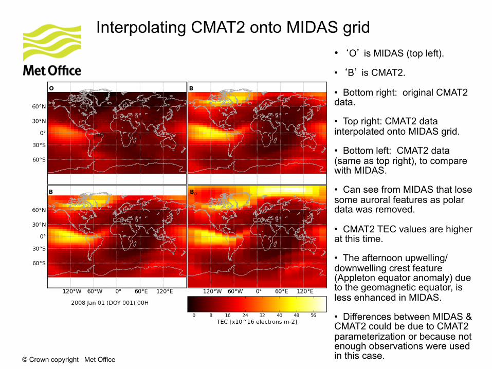
Interpolating CMAT2 onto MIDAS grid •  ‘O’ is MIDAS (top left).

•  ‘B’ is CMAT2.

•  Bottom right: original CMAT2 data.

•  Top right: CMAT2 data interpolated onto MIDAS grid.

•  Bottom left: CMAT2 data (same as top right), to compare with MIDAS.

•  Can see from MIDAS that lose some auroral features as polar data was removed.

•  CMAT2 TEC values are higher at this time.

•  The afternoon upwelling/ downwelling crest feature (Appleton equator anomaly) due to the geomagnetic equator, is less enhanced in MIDAS.

•  Differences between MIDAS & CMAT2 could be due to CMAT2 parameterization or because not enough observations were used in this case.


•  Histograms help to (1) find unphysical values, biases, & spikes in obs (2) give parameters used in QC, (3) choose sensible colour limits for plots. •  Checked data for Jan, Feb, Mar ’08. •  X-axis: TEC, Y-axis: number of grid points (log scale). •  Top left: B (CMAT2) has many more large TEC values. O (MIDAS) has -ve values. QC1 is to remove these unphysical –ve values. •  Top right: When each CMAT2 value is subtracted from equivalent MIDAS value, O-B is negative, showing CMAT2 values are usually larger than MIDAS, i.e. there’s a net -ve bias in (O-B). •  Bottom left: QC2, the relative difference, (O-B)/B, is a background check to ensure CMAT2 won't crash when feeding in observations which are very different from the model background. Isn’t too bad but is skewed –ve (so occurring at large B values). •  Bottom right: QC3, buddy check. To express how far each observation is from average of its neighbours, in terms of sigma (std dev). Removes outliers, i.e. checks that observations don't have unphysical spikes.

Quality control (QC)


•  Top left 4 slides are same as previous but here have limited TEC values to >0 so can see (blue pixels) –ve MIDAS at pole. •  Bottom left: O-B is generally blue so TEC values from CMAT2 are generally bigger than MIDAS (i.e. background is more +ve than MIDAS. White is agreement.

•  In O-B can see equatorial anomaly feature. Can see in CMAT2 but not MIDAS. CMAT2 has better latitudinal resolution. Require more stations at equator for MIDAS to pick out feature.

•  Hint of S American Weddell Sea anomaly on MIDAS (regional study required).

•  Bottom middle: relative difference (O-B)/B.

•  Top right: green pixels are values which were removed by QC check i.e. (1) removal of –ve polar values, (2) where departure from background is too great [i.e. if (O-B)/B was +/-50% then was removed] & (3) spikes >6sigma.

Before & after QC


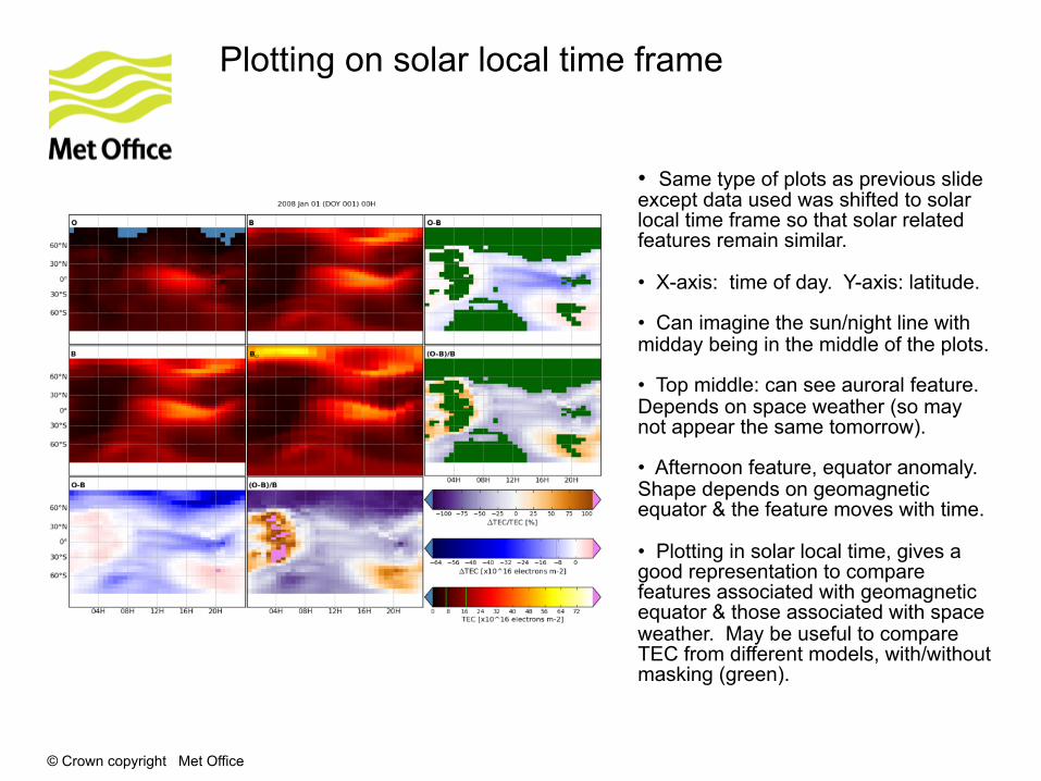
•  Same type of plots as previous slide except data used was shifted to solar local time frame so that solar related features remain similar.

•  X-axis: time of day. Y-axis: latitude. •  Can imagine the sun/night line with midday being in the middle of the plots. •  Top middle: can see auroral feature. Depends on space weather (so may not appear the same tomorrow). •  Afternoon feature, equator anomaly. Shape depends on geomagnetic equator & the feature moves with time. •  Plotting in solar local time, gives a good representation to compare features associated with geomagnetic equator & those associated with space weather. May be useful to compare TEC from different models, with/without masking (green).

Plotting on solar local time frame


•  Shows for each of the different thresholds which are set, how much data is retained as a percentage of overall data.

•  White shows little data. Dark shows most data. Green is no data.

•  Left hand side: geographical frame.

•  Right hand side: solar local time frame.

•  If MIDAS value is not within 25% of background value then it’s removed. So 25% threshold is harsh. Less data at 25% but more agreement between CMAT2 & MIDAS.

•  At the 75% threshold more data is retained but less agreement.

•  Most data is retained in the sub-tropical regions.

•  Most data is removed in the northern winter pole. Probably due to no observations at the pole for MIDAS or differences in climatology or CMAT2 / MIDAS may not be correct.

Varying threshold of QC2 (background check)


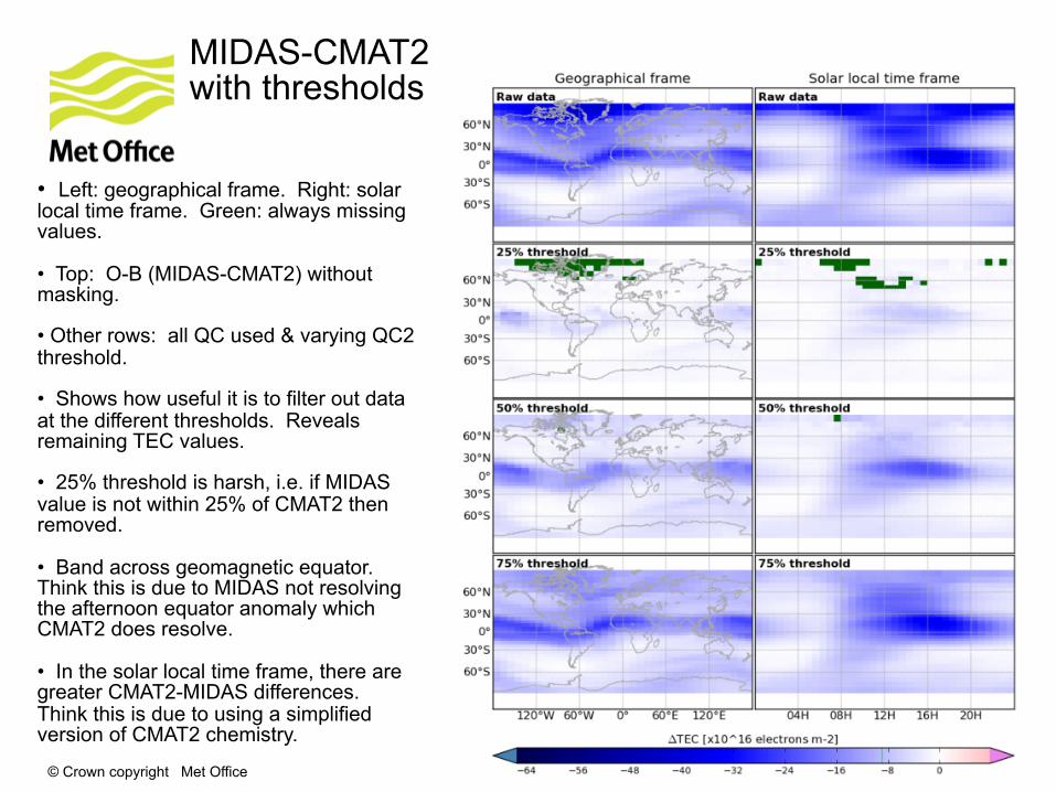
•  Left: geographical frame. Right: solar local time frame. Green: always missing values.

•  Top: O-B (MIDAS-CMAT2) without masking.

•  Other rows: all QC used & varying QC2 threshold.

•  Shows how useful it is to filter out data at the different thresholds. Reveals remaining TEC values.

•  25% threshold is harsh, i.e. if MIDAS value is not within 25% of CMAT2 then removed.

•  Band across geomagnetic equator. Think this is due to MIDAS not resolving the afternoon equator anomaly which CMAT2 does resolve.

•  In the solar local time frame, there are greater CMAT2-MIDAS differences. Think this is due to using a simplified version of CMAT2 chemistry.

MIDAS-CMAT2 with thresholds


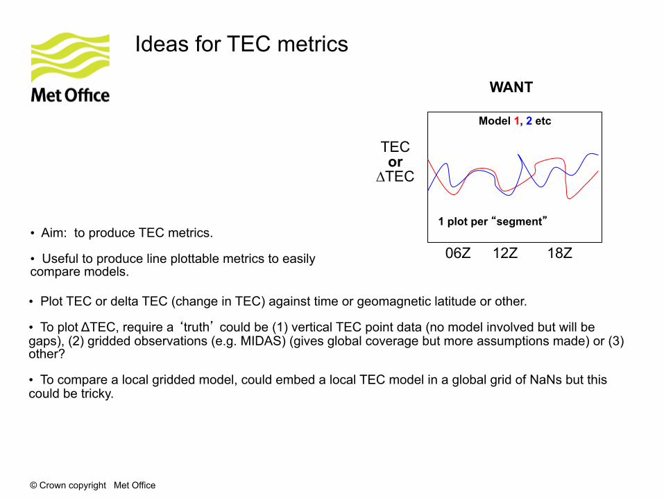
Ideas for TEC metrics

WANT

06Z 12Z 18Z

TEC or

∆TEC

Model 1, 2 etc

1 plot per “segment”

•  Plot TEC or delta TEC (change in TEC) against time or geomagnetic latitude or other.

•  To plot ΔTEC, require a ‘truth’ could be (1) vertical TEC point data (no model involved but will be gaps), (2) gridded observations (e.g. MIDAS) (gives global coverage but more assumptions made) or (3) other?

•  To compare a local gridded model, could embed a local TEC model in a global grid of NaNs but this could be tricky.

•  Aim: to produce TEC metrics.

•  Useful to produce line plottable metrics to easily compare models.


Ideas for TEC metrics (continued)

1 2 3 4

5

5 6

7

8

9

•  As TEC is sensitive to solar (F10.7) & geomagnetic (Kp) activity, probably want to segment up, to study.

•  Could also plot using different sectors: 1.  Geomagnetic (geographic?) latitude (N/S pole, N/S mid-latitude, equatorial sectors),

2.  Local time (day/night, afternoon sectors, etc),

3.  Combination of above (dayside equatorial),

4.  Go directly for features (equatorial anomaly, auroral features, etc).


Summary

•  MIDAS produces TEC maps from the delay in GPS signals.

•  CMAT2 is a model of the coupled middle atmosphere & thermosphere.

•  The two were compared to explore the assimilation of TEC data into CMAT2.

•  The study involved QC of the data. (1) removing unphysical –ve TEC values in MIDAS, (2) removing MIDAS values too far from CMAT2 values (& showing results of applying different thresholds), (3) removing spikes in MIDAS data by comparing values with nearest neighbouring values.

•  Auroral & equatorial features were identified when global maps were compared.

•  Some ideas for line plot TEC metrics include segmenting data in solar local time frame or geomagnetic latitude to view TEC or change in TEC.


Thank you. Questions and answers


Notes


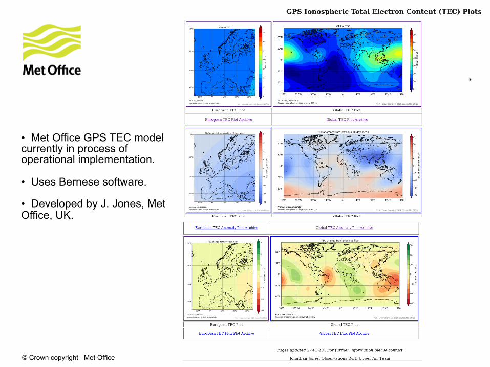
•  Met Office GPS TEC model currently in process of operational implementation.

•  Uses Bernese software.

•  Developed by J. Jones, Met Office, UK.


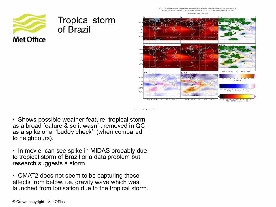
•  Shows possible weather feature: tropical storm as a broad feature & so it wasn’t removed in QC as a spike or a ‘buddy check’ (when compared to neighbours). •  In movie, can see spike in MIDAS probably due to tropical storm of Brazil or a data problem but research suggests a storm.

•  CMAT2 does not seem to be capturing these effects from below, i.e. gravity wave which was launched from ionisation due to the tropical storm.

© Crown copyri ght M et Of f ice

Tropical storm of Brazil


•  CMAT2: Parameterised models include: High latitude electric field model (Foster, Weimer, SuperDARN), Low latitude electric field model (Richmond), Particle Precipitation model (TIROS), Gravity wave schemes (e.g. Hybrid Lindzen-Matzuno parameterisation). •  High latitude auroral precipitation (including the effect of medium energy electrons) is from the TIROS/NOAA auroral precipitation statistical model. •  Electron density is from the Parameterized Ionospheric Model (PIM) which gives a good representation of densities at high latitudes. •  PIM, Parameterised Ionospheric Model: fast global ionospheric & plasmaspheric model based on a combination of the parameterised output of several regional & theoretical ionosphere models & an empirical plasmaspheric model. http://www.cpi.com/products/pim.html. •  Lower boundary 16km tidal forcing from the Global Scale Wave Model (GSWM). Although Edmund used 80km mode so no tidal forcing came into it.

CMAT2


•  CMAT2 Chemistry: Neutrals O, O2, N2 (15 minor species). Ions O+, O2+, NO+ (15 minor species).

•  Lower boundary seasonal forcing from MSISE90 (an NRL mass spectrometer, incoherent scatter radar extended empirical model) or Stratospheric Sounding Unit satellite data (geopotential height instrument on board NOAA-12 & NOAA-14 satellites).

•  Gravity wave drag & geomagnetic activity index (kp) are used.

•  Output: either real-time graphical output or post-run plotting

•  Thermospheric heating, photodissociation & photoionization are calculated due to absorption of solar X-ray, EUV & UV radiation between 0.1-194nm.

•  Mesospheric heating is calculated due to absorption of solar radiation by ozone, oxygen & exothermic neutral chemistry.

•  Radiative cooling parameterisations included are: 9.6m NO emission, 63m atomic oxygen emission, 15.6m CO2 emission,03 9.6m radiative emission.

CMAT2


•  To see relative contribution of different quality control filters. •  Buddy check includes removing unphysical-most. Only removes 2 extra points – one in Arctic where not enough neighbours for an average, another where obs dips near Antartica. •  Buddy doesn't remove weather feature (above Brazil, probably due to gravity waves from tropical storm)) as it's extended & not a spike. •  But background check does remove feature at all values. •  Lots removed at north pole •  Left column: MIDAS, CMAT2, MIDAS-CMAT2. •  Top row: Background check at different thresholds, e.g. if MIDAS-CMAT2>25% then removed. •  Plots showing ‘buddy check’ (comparison with neighbouring values), set at 6sigma. •  Green are the pixels which have been removed after a buddy check. •  Top row: MIDAS, MIDAS-CMAT2 with 25% threshold (harsh), 50% threshold (OK), 75% threshold (generous). •  Middle row: CMAT2, different thresholds for relative change. •  Bottom row: Difference between MIDAS & CMAT2, relative change, buddy check & without a threshold. •  Can see spike removal (70E, 50S) in bottom row, 3rd image along.

Buddy check (QC3) & thresholding (QC2)


MIDAS (O) CMAT2 (B)

Average QC'd JFM MIDAS & CMAT2 Left: MIDAS. Right:CMAT2. Average of data in JFM 2008. Left sides: geographical frame. Right sides: solar local time frame. Top: raw data. Below: using different thresholds for background check (QC2).

cmat2 / midas comparison · pdf filesystem which performs 3d tomography of the ionosphere....

Documents