clustering patterns of urban built-up areas with … patterns of urban built-up areas with curves of...

$: Clustering patterns of urban built-up areas with … patterns of urban built-up areas with curves of fractal scaling behaviour Isabelle ... the spatial organization of an urban pattern$
1 IntroductionThe analysis of urban built-up areas is a fascinating and complex topic (Batty, 2005;Conzen, 2001; Levy, 1999). Fractals have considerable potential for describing, meas-uring, analyzing, and modelling complex realities, whatever the field of application(ecology, physics, remote sensing, etc) (eg see Halley et al, 2004). An interestingaspect of fractals for urban geographers is their ability to summarize the complexity,compactness, and heterogeneity of a spatial distribution in a single value (the fractaldimension, denoted D) that is independent of scale (eg see Batty, 2005; Frankhauser,1998a; 2008; Lam and de Cola, 2002; Lorenz, 2003; Salingaros, 2003).

In this paper we discuss the use of a less common fractal output: the curve ofscaling behaviour, which may provide interesting spatial information about theorganization of urban patterns at different scales. The curve of scaling behaviour iscomplementary to the fractal dimension, which is a more global index. When com-puting curves for several built-up areas, it is interesting to compare their shapes notonly visually but also quantatively. In this paper we suggest the use of a k-medoidalgorithm for this purpose (section 2.3) and apply the method to forty-nine Europeanwards (section 3). The curve of scaling behaviour is seen as an interesting complemen-tary morphometrical measurement, a local index of morphology. Both indicators(fractal dimension and curve of scaling behaviour) should be part of the geographer'stoolbox for exploratory spatial data analysis of urban morphologies.

Clustering patterns of urban built-up areas with curvesof fractal scaling behaviour

Isabelle ThomasFRS-FNRS, CORE, and Department of Geography, Universite catholique de Louvain,Voie du Roman Pays, 34 B-1348, Louvain-la-Neuve, Belgium;e-mail: [email protected]

Pierre FrankhauserTHEMA (CNRS UMR 6049), Universite de Franche-Comte, Besanc° on, France;e-mail: [email protected]

Benoit FrenayMachine Learning Group, Universite catholique de Louvain, Louvain-la-Neuve, Belgium;e-mail: [email protected]

Michel VerleysenMachine Learning Group, Universite catholique de Louvain, Louvain-la-Neuve, Belgium;and SAMOS-MATISSE, Universite Paris 1 Pantheon-Sorbonne, Paris, France;e-mail: [email protected] 23 March 2009; in revised form 19 October 2009; published online 28 June 2010

Environment and Planning B: Planning and Design 2010, volume 37, pages 942 ^ 954

Abstract. Fractal dimension is an index which can be used to characterize urban areas. The use ofthe curve of scaling behaviour is less common. However, its shape gives local information about themorphology of the built-up area. This paper suggests a method based on a k-medoid for clusteringthese curves. It is applied to forty-nine wards of European cities, and shows that the curves addinteresting intraward information to our knowledge of the spatial variation of the urban texture.Moreover, morphological similarities are observed between cities: living, architectural, and planningtrends are not specific to individual cities.

doi:10.1068/b36039

Our results differ from those presented by Thomas et al (2009) where the fractaldimension was `simply' measured on a larger set of urban wards; it made no referenceto curves of scaling behaviour. The two papers are methodologically complementary.

2 Methodological aspectsBinary images are used here: black pixels correspond to built-up areas and white pixelsto open spaces.We tested whether the spatial distribution of the black pixels followeda fractal law. A practical example of output is presented in the appendix. The fractaldimension is first explained (section 2.1), and then the curve of scaling behaviour(section 2.2) is considered. Section 2.3 presents a method for clustering placesaccording to the shape of their curve of scaling behaviour.

2.1 Fractal dimension(s)Fractal dimension is a quantity indicating how completely a fractal fills the space beingstudied as one zooms down to finer and finer scales. There is no unique way of definingand estimating the fractal dimension (D); here it is computed by means of a correlationanalysis (eg see Grassberger and Procaccia, 1983). A small square window of size esurrounds each built-up pixel. The number of built-up pixels in each window is thencounted, which allows the mean number of pair correlations N(e) per window to becomputed. This operation is repeated for windows of different sizes. This results in aseries of measurements that can be represented on a Cartesian graph, where the X-axisis the size of the window e, and the Y-coordinate is the mean number of points perwindow (see the appendix).

The next step consists of fitting this empirical curve to a theoretical curvethat corresponds to a fractal law; that is, a power law which links the number ofcorrelations to the size of the window:

N�e� � aeD , (1)

where a is the prefactor of shape, and summarizes the nonfractal morphologicalproperties of the geometric object being analyzed (for a discussion see eg, Frankhauser,1998b; Gouyet, 1996; Thomas et al, 2009). It can be interpreted as a synthetic indicatorof the local particularities of the pattern across scales, due mainly to the fact that theelements of the built-up structure do not have the same shape. For instance, the sizesof the buildings in a residential area (such as detached houses) differ from the sizes ofthose in an industrial zone. Hence, even if the scaling behaviour and the fractaldimension are the same for both patterns, the mass N(e) differs because the baselengths of the buildings are different. The meaning of a becomes clearer when theidentity a � bD is introduced into equation (1):

N�e� � aeD � bDeD � �be�D � �e 0 �D � N�e 0 � .

In a sense, b corresponds to the average base length of the buildings, which are theconstitutive elements of the urban patterns. Differences in b-values also appear when twopatterns that have been digitized in different ways are compared; that is, when the sizes ofthe pixels differ. Hence, in this study the size of the pixel was controlled and fixed at 4m.

In real-world patterns, fractal behaviour can change across scales. Frankhauser(1998a; 2008) has shown that such changes often occur within rather small ranges of e,especially for small distances corresponding to the size of small blocks of houses orcourtyards. He suggested the introduction of an additional parameter c that allowsthe estimation of D and a by acting on the overall position of the power-law curve.The enlarged fractal then becomes:

N�e� � aeD � c . (2)

Clustering patterns of urban built-up areas 943

A nonlinear regression is here used for estimating a, D, and c that best fit the empiricalcurve (appendix).

The fractal dimension of a built-up area can take any value between 0 and 2.When D � 2 the built-up pattern is uniformly distributed. D � 0 corresponds to alimiting case in which the pattern is made up to one single point (eg a single farmbuilding surrounded by fields). D < 1 corresponds to a pattern of disconnectedelements (a number of built-up clusters separated one from another). D > 1 indicatesconnected elements (1) forming large and small clusters, in which isolated elementsmay also occur. The closer D is to 2, the more the elements are connected to eachother and belong to one single large cluster. From experience, we know that Dprovides quite a good indicator of the morphology of a built-up area (eg see Batty,2005; De Keersmaecker et al, 2003). The absolute value of D is slightly influencedby the estimation technique, the size of the window, and the centring of the window,but these factors do not affect the relative variations and operational conclusions(eg see Thomas et al, 2007).

2.2 Curve of scaling behaviourIn this section we introduce an alternative representation of the empirical results of afractal analysis: the `curve of scaling behaviour' (Frankhauser, 1998a). Palmer (1988)called this a `fractogram', but this terminology is limited to ecology (Leduc et al,1994). In urban analysis the curve of scaling behaviour has been used up to now onlyfor defining critical scales where the fractal behaviour changes; it has often beenused to redefine the size of the window (see Frankhauser, 1989a; 1998b; 2004; Tannierand Pumain, 2005). Batty (2001) used this type of representation, which he called`signature', to analyze simulated urban patterns.

In this paper we consider the potential use of the curve of scaling behaviour forfurther characterizing the morphology of urban areas. Let us recall the underlyinglogic of this type of representation. For this purpose, we start with the original fractallaw in equation (1). Taking the logarithm (2) of this relation yields

logN�e� � log a�D log e ,

which corresponds to a linear relationship between logN(e) and log e. Hence, we obtain

d logN�e�d log e

� D ,

where D corresponds to the constant slope value in the linear relation. However, asalready pointed out, the fractal dimension may depend on the scales of the real-worldpatterns. Then D becomes a function of the scale e [that is, D � D(e)]. It is also possiblethat the typical shape of the objects depends on the scale. In this case this wouldmean that the shapes of house blocks or town sections are not the same as those ofbuildings, which implies that the prefactor a is a function of e.

If we assume that the prefactor a and the fractal dimension D both depend on thedistance parameter, we obtain:

logN�e� � log a�e� �D�e� log e ,

and thus the variation of logN(e) with respect to log e becomes (Frankhauser, 1998a):

d logN�e�d log e

� a�e� � d log a�e�d log e

� dD�e�d log e

log e�D�e� . (3)

(1) In this paper, connectivity is always considered from a fractal point of view.(2) The symbol log has been used since the base of the logarithm does not matter in the given context.

944 I Thomas, P Frankhauser, B Frenay, M Verleysen

According to equation (3), a(e) is equal to a constant D-value, if neither a nor Ddepend on e. However, two additional terms contribute to a(e): one refers to variationsin the shape of the elements which do not affect the fractal behaviour (that is, thehierarchical organization of the pattern) and the other describes the changes of fractalbehaviour across scale.(3) Due to these terms, the a-values may exceed the upper limitvalue of D � 2.

Parameter a(e) describes the relative changes in the built-up mass N(e) with respectto the relative change in the distance. Indeed given that

d logN�e� � dN�e�N�e� ; d log e � de

e,

we obtain

a�e� � d logN�e�d log e

��dN�e�N�e�

��dee

�.

This is a generalization of the usual allometric relationship that is typical of fractals.Empirical curves of scaling behaviour a(e) doöof courseönot allow distinguishing

between the two types of contributions to equation (3); that is, the variation of a(e) andthat of D(e). We may, however expect they provide detailed information to what extentthe spatial organization of an urban pattern changes across scales or remains constant.Experience shows that the variation of a(e) and D(e) usually do not affect the qualityof the fit between the empirical curve and the estimated curve (2). Indeed, whenmeasuring the quality of adjustment between the empirical curve and the estimatedcurve by an R 2 coefficient, we consider the fit between the two curves as `poor' whenR 2 < 0:9999; in these cases, we can either conclude that the studied pattern is notfractal, or that it is multifractal (see Tannier and Pumain, 2005). Hence fractaldimension plays the role of a still-valid mean indicator for scaling behaviour.

2.3 Clustering curvesThe shape of the curve of scaling behaviour a(e) reveals intraward spatial structures.By visually comparing the curves, we can distinguish different types of shapes, but it isnot obvious either how to find objective criteria for defining homogeneous groups ofcurves, nor how to set the number of groups. This question is a rather standardquestion in data analysis, and is known under the name clustering. Clustering consistsof grouping data together according to some appropriate criterion; in our case theobjects are the curves of scaling behaviour, and the criterion is shape similarity.

Methods traditionally used by geographers are here not applicable: linear correla-tion does not assess the resemblance between two shapes. The relationship betweentwo shapes can be nonlinear (horizontal or vertical shifts, rotations, etc), whereascorrelation measures only linear relationships. Other methods better known in statisticsand data analysis overcome this limitation. Among them, the most widely known andused is probably the k-means algorithm. The k-means algorithm consists in (i) findinggroups (called clusters) of objects (here: curves) that are similar (here: in shapes),and (ii) for each group finding a representative, which is usually simply the meanöor centre of gravity or centroidöof the objects.

However, the k-means suffers from a drawback which concerns the interpretability ofthe results: the centroid of experimental data is often not one of the experimental data.

(3) Remember that we assume here that c is a global parameter which does not vary with scale.It may be interpreted as a general error term which summarizes other random errors. Then we mayrewrite the relationship N(e) � aeD � c simply as N(e)ÿ c � N0(e) � aeD � c, which allows us toproceed to the subsequent steps.


Therefore, we here use a slightly different version of k-means which is called k-medoid,where the representative of each cluster is forced to be one of the initial pieces of dataforming the cluster. As an example, let us imagine for the simplicity of the representa-tion that the data are two-dimensional objects; that is, points in a two-dimensionalspace, instead of curves. Figure 1 shows the difference between the centroid and themedoid of the cluster formed by the six illustrated data points: the centroid is the pointin the space which is on average closest to each datapoint, while the medoid is thedatapoint from the initial set which is on average closest to the other datapoints.

The k-medoid algorithm (Bishop, 2006) works as follows. Given a set of curvesa1 , . . . , an , the k-medoid algorithm produces a clustering C � fC1 , . . . , Cmg where them clusters are characterized by the medoids g1 , . . . , gm . These medoids are chosen fromthe n curves: Ck contains the curves that are closer to gk than to any other medoid.More precisely, this algorithm finds the minimum of the function

J�C� �Xmk� 1

J�Ck � �Xmk� 1

Xai 2Ck

d�ai , gk )2 , (4)

where d(ai , gk ) is the dissimilarity between the curve ai and the medoid gk . Finding theminimum of equation (4) gives a set of m medoids that best represent the set of ncurves a1 , . . . , an into m clusters. To find the minimum of equation (4), the k-medoidalgorithm proceeds into two steps: it first computes the dissimilarity d(ai , aj ) betweeneach pair of curves ai and aj , and then it minimizes J(C).

Let us first consider the computation of the dissimilarity d(a, a 0 ) between the twocurves a � (a 1, . . . , aT ) and a 0 � (a 01, . . . , a 0T ) where a 0 is the ith point of a. A simplesolution (see figure 2) is to define

d�a, a 0� �XTi� 1

�a i ÿ a 0i �2 , (5)

4

3

2

5

6

1

Datapoint

Medoid

Centroid

Figure 1. The difference between a centroid and a medoid.

a 0

a

Figure 2. Naive matching between two a-curves.


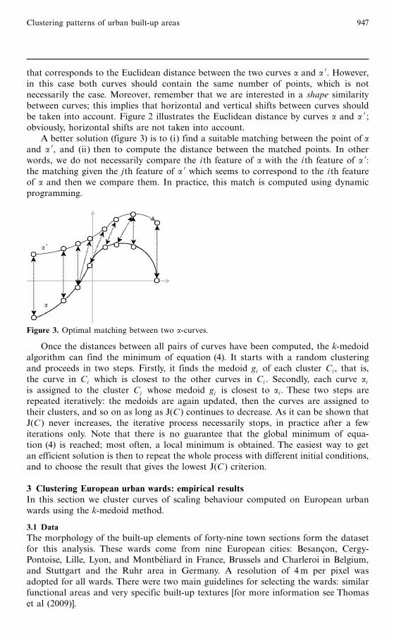
that corresponds to the Euclidean distance between the two curves a and a 0. However,in this case both curves should contain the same number of points, which is notnecessarily the case. Moreover, remember that we are interested in a shape similaritybetween curves; this implies that horizontal and vertical shifts between curves shouldbe taken into account. Figure 2 illustrates the Euclidean distance by curves a and a 0 ;obviously, horizontal shifts are not taken into account.

A better solution (figure 3) is to (i) find a suitable matching between the point of aand a 0, and (ii) then to compute the distance between the matched points. In otherwords, we do not necessarily compare the ith feature of a with the ith feature of a 0:the matching given the jth feature of a 0 which seems to correspond to the ith featureof a and then we compare them. In practice, this match is computed using dynamicprogramming.

Once the distances between all pairs of curves have been computed, the k-medoidalgorithm can find the minimum of equation (4). It starts with a random clusteringand proceeds in two steps. Firstly, it finds the medoid gi of each cluster Ci , that is,the curve in Ci which is closest to the other curves in Ci . Secondly, each curve aiis assigned to the cluster Cj whose medoid gj is closest to ai. These two steps arerepeated iteratively: the medoids are again updated, then the curves are assigned totheir clusters, and so on as long as J(C) continues to decrease. As it can be shown thatJ(C) never increases, the iterative process necessarily stops, in practice after a fewiterations only. Note that there is no guarantee that the global minimum of equa-tion (4) is reached; most often, a local minimum is obtained. The easiest way to getan efficient solution is then to repeat the whole process with different initial conditions,and to choose the result that gives the lowest J(C) criterion.

3 Clustering European urban wards: empirical resultsIn this section we cluster curves of scaling behaviour computed on European urbanwards using the k-medoid method.

3.1 DataThe morphology of the built-up elements of forty-nine town sections form the datasetfor this analysis. These wards come from nine European cities: Besanc° on, Cergy-Pontoise, Lille, Lyon, and Montbeliard in France, Brussels and Charleroi in Belgium,and Stuttgart and the Ruhr area in Germany. A resolution of 4m per pixel wasadopted for all wards. There were two main guidelines for selecting the wards: similarfunctional areas and very specific built-up textures [for more information see Thomaset al (2009)].

a 0

a

Figure 3. Optimal matching between two a-curves.


We limit ourselves to considering built-up areas, without knowing the exact functionof the buildings (residential, service, industrial, etc). The open spaces (white pixels)are considered as lacunae or `green areas' (see section 1).We know that there is a biashere that we could not avoid: these open areas or empty cells include roads. In orderto minimize this bias, we avoided choosing wards containing large transportationinfrastructures, such as railway stations or major roads.

A window was specified around each urban section in such a way that it includedthe built-up area that had been visually selected; the fractal dimension was computedon this window.Very small windows were avoided, following the principle that the errorincreases as the number of observations falls; the ratio between the size of the objectand that of the window is always smaller than 1, in order to avoid measuring artefacts.

A measuring protocol was defined and applied. This ensured rigorous control ofthe quality of the estimate and avoided measurement artefacts (De Keersmaecker et al,2003; Thomas et al, 2009). The same method, with the same control parameters andthe same threshold values, was used for all the windows.

3.2 Fractal analysisThe fractal dimension in this dataset (n � 49) has an average value of 1.84 and mostof the observed values are higher than 1.75 (figure 4). High D-values indicate that thebuilt-up area is homogeneous at different scales, while small D-values reveal hetero-geneity: that is, variety in the built-up areas across scales. In our sample of wards,there is some variation between urban wards. Overall, the wards are globally quitehomogeneous: the value of the first quartile is very high (D � 1:92), and the valueof the median (1.86) is above the mean value. Large values of D are associated withsmall variations of a (figure 5) and R 2 (not illustrated here). The a-values are herealways smaller than 2, confirming the fractal nature of the phenomenon. Asexpected, R 2 is always higher than 0.9999 and increases with D: the higher the valueof D, the denser and more homogeneous the built-up area (that is, the larger itsmass), and, hence, the more urbanized it is (see also Frankhauser, 2008; Thomaset al, 2007). These first results correspond to our expectations: the history andgeography of the city matter, and no clear-cut country effect is visible (see Thomaset al, 2009).

15

10

5

0

Frequency

1.5 1.6 1.7 1.8 1.9 2.0D

Mean: 1.835Standard deviation: 0.113

Figure 4. Statistical distribution of D.

1.5

1.0

0.5

a

1.6 1.7 1.8 1.9 2.0D

Figure 5. Relationship between fractal dimension(D) and prefactor (a).


As figure 5 suggests, even if D reveals the homogeneity/heterogeneity of built-upspace, by itself it is not sufficient to discriminate univocally between two spatialorganizations. Different patterns can lead to the same value of D, and a given valueof D may correspond to different spatial patterns [for a demonstration see Thomaset al (2007)]. Hence D can only be considered as kind of general index.

3.3 Clustering curvesIn spatial analysis it is interesting not only to characterize the morphology of eachpattern by one or several indices (section 3.2), but also to see whether some placeslook alike and why (historical or geographical circumstances). For instance, weexpect settlements which grew up during early periods of industrialization tohave different patterns from medieval centres or 20th-century new towns. Recentobservations seem to confirm such hypotheses (eg see Frankhauser, 2004; 2008;Salingaros, 2003; Thomas et al, 2007; 2008a; 2008b). The aim here is to cluster wardson the basis of the shape of their curve of scaling behaviour. In other words, a curvesuch as that illustrated in figure A3 in the appendix should be clustered with allother curves having the `same' shape: that is to say curves with a minimum valueat low distances, even if this minimum is placed slightly further farther left or right.This last condition makes the problem trickier than simply the computationof a correlation distance. It was tackled using the k-medoid method described insection 2.3.

Figure 6 shows the value of J(C) for different numbers of clusters (k). J(C )decreases as k increases, so that there is no formal criterion for choosing k. For thispaper we chose k � 5, as a compromise between model error and model complexity.The left column in figure 7 gives the composition of the clusters in terms of curves,while the right column gives one example for each cluster (either the medoid or thearea that was visually the most typical).

Let us now compare the clusters in terms of J(C). For better comparison, we willuse the square root of the value divided by the number of curves in the cluster, andlabel this AdjJ(C). AdjJ(C) indicates the average dissimilarity between an a-curveand the medoid of the cluster to which it has been assigned (table 1). The highestvalues of AdjJ(C) are observed for clusters 2 and 3. This means that the curves inthese clusters are the most diverse (see also figure 7), while clusters 0, 1, and 4 consist

1.0

0.8

0.6

0.4

0.2

0.0

J(C)

0 10 20 30 40 50

Number of clusters, k

k � 5

Figure 6. The relationship between J(C ) and the number of clusters, k.


of curves that look more alike. Surprisingly, these last three groups also have highD-values (figure 8).

Clusters 0 and 4 have the highest average D values (D > 1:7) (figure 8); theycorrespond to more or less classic' densely urbanized areas. They often correspond tocity centres with root-like built-up patterns (see section 2.2). However, the shape of thescaling curves is different in clusters 0 and 4 (see the left column of figure 7), due todifferences in the structure of the built-up areas (right column of figure 7). The analysisof the curves of scaling behaviour has thus provided detailed information about thespatial organization of the urban fabric, since the variation in the fractal behaviouracross scales is taken into account.

By looking in more detail at the features of the wards, we can see that cluster 0corresponds to detached houses aligned along roads (regular organization). Thedistances between the buildings are small, but white pixels (open spaces) betweenthe buildings are quite numerous. This explains the substantial drop in the scalingbehaviour at short distances (figure 7, left). As pointed out above, parameter a linksthe relative variation in the built-up areas to that of distance, and in cluster 0 therelative variation is low at short distances. This type of fabric often characterizesthe suburbs of cities. Cluster 4 has similar D-values to cluster 0 (see figure 8), but avisually different built-up morphology: the curves are much flatter (less variation)and the buildings are more densely packed. They are often terraced. Cluster 4 mostlyconsists of dwellings in old city centres, mixed with some larger buildings used asoffices, schools, shops, etc.

Cluster 2 is heterogeneous in terms of the scaling curves (table 1). There are onlythree urban wards in this cluster, and they have atypical scaling curves (figure 7).All three come from the new town of Cergy-Pontoise in France, which was createdin 1969 to manage the development of the Paris Region in terms of habitat, activities,transport, etc. Cergy-Pontoise has avoided both the role of industrial centre and thatof dormitory town, and has succeeded in maintaining the balance between places ofwork, culture, and habitation. This has led to a certain diversity in its built-up areas,as illustrated in figure 7, with a mixture of large apartment blocks (barres) and smalldetached houses (pavillonnaires).

Cluster 3 corresponds to `pure' Corbusian built-up areas. It consists of socialhousing (apartment blocks), in quite uniform and regular formations. In France theseare called Les Grands Ensembles.

Last but not least, cluster 1 consists of areas with buildings covering largeirregular areas. These are mainly free-standing industrial or office buildings, whereintrabuilding distances are considerable. As illustrated by the curves in figure 7,the scaling behaviour is large at small distances due to the size of the buildings.

Table 1. AdjJ(C ) for the five clusters.

Cluster AdjJ(C )

0 0.08781 0.06682 0.11363 0.10264 0.0773


Curves of scaling behaviour Examples

Cluster 0

Cluster 1

Cluster 2

1.8

1.6

1.4

1.2

1.0

1.8

1.6

1.4

1.2

1.0

1.8

1.6

1.4

1.2

1.0

a-value

a-value

a-value

Stutt04Besanc° an03Montbel04Stutt02Charleroi04Lyon07Lyon02Lyon05Bruxelles03Lille04Lille07Lille06Charleroi02Bruxelles05(M) Bruxelles04Montbel03Lille05Besanc° an04

(M) Stutt06Charleroi03Bruxelles06Lyon06Ruhr03

Cergy01(M)Cergy03Cergy04

0 5 10 15 20 25 30

0 5 10 15 20 25 30

0 5 10 15 20 25 30

Scale id

Scale id

Scale id

Brussels 04

Brussels 06

Cergy-Pontoise 01

Figure 7. Cluster composition when k � 5: curves and one example of each type of urbanstructure.


Cluster 3

Cluster 4

1.8

1.6

1.4

1.2

1.0

1.8

1.6

1.4

1.2

1.0

a-value

a-value

0 5 10 15 20 25 30

0 5 10 15 20 25 30

Scale id

Scale id

(M) Besanc° an02Stutt03Stutt08Montbel02Cergy02Lyon04Lille02

Stutt05Besancon01Stutt07Stutt01Montbel01Lyon01Lille08Bruxelles02Bruxelles01Charleroi01Lille01(M) Lille03Charleroi05Lyon03Ruhr04Ruhr02Ruhr01

Besanc° on 02

Lille 03

Figure 7 (continued).

2.0

1.9

1.8

1.7

1.6

0 1 2 3 4

D

Cluster

Figure 8. The distribution of the fractal dimensions, D, in each cluster.


4 ConclusionThis paper has considered scaling behaviour curves, an output of fractal analysis.These curves illustrate how the two fractal parameters vary across scales. Distanceranges can be identified at which substantial changes in spatial organization occur, oralternatively, for which the parameters are stable. Hence the information contained inthese curves turns out to be complementary to that of the fractal dimension D whichremains a useful, but rather general, indicator.

An important contribution of this paper is the use of the k-medoid method tocluster the curves of similar shapes. This method is quite similar to that of k-means,but can use dissimilarity measures which are not distances. Here, it allows a dissim-ilarity to be computed from a matching, which is well suited to curves with horizontalor vertical shifts. It is useful not only for curves of fractal scaling behaviour but also forclustering any other curves in geography (remote sensing, etc). The application to a setof European urban wards showed that the clustering results fit well with planninghistory (areas with similar histories cluster together). Clustering the curves instead ofusing only the fractal dimension undoubtedly adds accuracy to the final result in termsof morphometry.

ReferencesBatty M, 2001, `Generating urban forms from diffusive growth'' Environment and Planning A 23

511 ^ 544Batty M, 2005 Cities and Complexity: Understanding Cities with Cellular Automata, Agent-based

Models, and Fractals (MIT Press, Cambridge, MA)Bishop C, 2006 Pattern Recognition and Machine Learning (Springer, Berlin)Conzen M, 2001, ``The study of urban form in the United States'' Urban Morphology 5(1) 3 ^ 14De Keersmaecker M L, Frankhauser P, Thomas I, 2003, ` Using fractal dimensions to characterize

intra-urban diversity: the example of Brussels'' Geographical Analysis 35 310 ^ 328Frankhauser P, 1998a, ` The fractal approach: a new tool for the spatial analysis of urban

agglomerations'' Population 4 205 ^ 240Frankhauser P, 1998b, ` Fractals geometry of urban patterns and their morphogenesis'' Discrete

Dynamics in Nature and Society 2 127 ^ 145Frankhauser P, 2004, ` Comparing the morphology of urban patterns in Europeöa fractal

approach'', in European Cities: Insights on Outskirts Eds A Borsdorf, P Zembri (ESF COSTOffice, Brussels) pp 79 ^ 105

Frankhauser P, 2008, ``Fractal geometry for measuring and modelling urban patterns'', inThe Dynamics of Complex Urban Systems: An Interdisciplinary Approach Eds S Albeverio,D Andrey, P Giordano, AVancheri (Physica, Heidelberg) pp 213 ^ 243

Gouyet J F, 1996 Physique et Structures Fractales 2nd edition (Masson, Paris)Grassberger P, Procaccia I, 1983, ` Measuring the strangeness of a strange attractor'' Physica D

9 189 ^ 208Halley J, Hartley S, Kallimanis A, KuninW, Lennon J, Sgardelis S, 2004, ` Uses and abuses of

fractal methodology in ecology'' Ecology Letters 7 254 ^ 271Lam N, de Cola L, 2002 Fractals in Geography (The Blackburn Press, Caldwell, NJ)Leduc A, Prairie Y, Bergeron Y, 1994, ` Fractal dimension estimates of a fragmented landscape:

sources of variability'' Landscape Ecology 9 279 ^ 286Levy A, 1999, ` Urban morphology and the problem of the modern urban fabric: some questions

of research'' Urban Morphology 32(2) 79 ^ 85Lorenz W, 2003, ` Fractals and fractal architecture'',Vienna University of Technology,

http://www.iemar.tuwien.ac.at/fractal architecture/subpages/01Introduction.htmlPalmer M, 1988, `Fractal geometry: a tool for describing spatial patterns of plant communities''

Vegetatio 75 91 ^ 102Salingaros N, 2003, ` Connecting the fractal city'', keynote speech, Biennial of Towns and Town

Planners in Europe, Barcelona, http://www.zeta.math.utsa.edu/�yxk833/connecting.htmlTannier C, Pumain D, 2005, ` Fractales et geographie urbaine: aperc° u theorique et application

pratique'' Cybergeo paper 307Thomas I, Frankhauser P, De Keersmaecker M L, 2007, ` Fractal dimension versus density of

the built-up surfaces in the periphery of Brussels'' Papers in Regional Science 86 287 ^ 307


Thomas I, Frankhauser P, Biernacki C, 2008a, ` The morphology of built-up landscapes inWallonia, Belgium: a classification using fractal indices'' Landscape and Urban Planning84 99 ^ 115

Thomas I, Tannier C, Frankhauser P, 2008b, ` Is there a link between fractal dimension andresidential choice at a regional level? '' Cybergeo paper 413

Thomas I, Frankhauser P, Badariotti D, 2009, ` Comparing the fractality of Europeanneighbourhoods: do national contexts matter? '', paper presented at the ERSA 2009conference in Lo« dz and at the ASRDLF 2009 in Clermont Ferrand; copy available from theauthors

AppendixExample of a fractal analysis using Fractalyse (http://www.fractalyse.org/) on a real-world urban area in Brussels (named Bruxelles04), Belgium.

20

15

10

5

0

1.9

1.8

1.7

1.6

1.5

1.4

1.3

4000

3000

2000

1000

0

Scalingbehaviour

Frequency

Empirical/estimatedD

0 50 100 150 0 50 100 150

ÿ4 ÿ2 0 2 4

Difference

Distance Distance

Figure A1. The studied area. Figure A3. Difference between observed andestimated values of D.

Figure A2. Empirical and estimated D-values(2 curves superimposed) according to distance.

Figure A4. Curve of scaling behaviour.

ß 2010 Pion Ltd and its Licensors


Conditions of use. This article may be downloaded from the E&P website for personal researchby members of subscribing organisations. This PDF may not be placed on any website (or otheronline distribution system) without permission of the publisher.

clustering patterns of urban built-up areas with … patterns of urban built-up areas with curves of...

Documents