cluster requiem and the rise of cumulative...
TRANSCRIPT

CLUSTER REQUIEM AND THE RISE OF CUMULATIVE GROWTH THEORY
by
Gary Monroe Kunkle
A dissertation submitted to the faculty of The University of North Carolina at Charlotte
in partial fulfillment of the requirements for the degree of Doctor of Philosophy in
Public Policy
Charlotte
2009
Approved by: Dr. Harrison Campbell Dr. Kent Curran Dr. John Kello
Dr. Suzanne Leland
Dr. Joseph Whitmeyer

ii
©2009 Gary Monroe Kunkle
ALL RIGHTS RESERVED

iii
ABSTRACT
GARY MONROE KUNKLE. Cluster Requiem and the Rise of Cumulative Growth Theory (Under the direction of DR. HARRISON S. CAMPBELL) Industry cluster theory has been the predominant model guiding economic development
policy throughout the world for nearly two decades. As appealing as the cluster approach has
been to regional scientists and policy makers it suffers from a number of theoretical and
empirical shortcomings, including an inability to explain economic dispersion and the presence
of high-growing firms that thrive in non-clustered industries and locations. This dissertation
tracks the growth and survival of a cohort of more than 300,000 establishments operating in
Pennsylvania during the 1997-2007 period. It reveals that firm characteristics are 10-times more
powerful than industry and cluster characteristics, and 50-times more powerful than location
characteristics, in explaining and predicting establishment-level growth and survival. It also
finds a Power Law is present in the distribution of establishment growth, indicating that a sub-
set of businesses systematically accumulate a disproportionate share of employment growth.
Roughly 1% of establishments created 169% of all net new jobs added in the state over a ten-
year period. Growth is further concentrated among businesses that are able to sustain growth
over multiple years. This suggests that the principal driver of regional growth is cumulative firm
growth – the accumulation of a disproportionate amount of growth among a small number of
firms through sustained expansion over multiple years. I conclude that the path to building
better theory and more effective development policies is one that explicitly links regional
growth to the growth of firms. Such an approach should focus on endogenous firm dynamics
rather than exogenous heuristics such as industry and location.

iv
ACKNOWLEDGEMENTS My personal thanks goes to Harry Campbell, my committee Chair, for his wise and patient
advice over the past five years, as well as to the members of my committee who have kindly
allowed the preparation of this dissertation to take a long and winding course. A special place in
my heart is reserved for my wife and partner, Monique Pelle Kunkle, who has never wavered in
her encouragement of my self-actualizing pursuits.

v
TABLE OF CONTENTS LIST OF FIGURES vii
LIST OF TABLES viii
CHAPTER 1: INTRODUCTION AND BACKGROUND 1
CHAPTER 2: LITERATURE REVIEW 12
2.1 Cluster Theory 13
2.1.1 Agglomeration Theory 17
2.1.2 Institutional Theory 18
2.1.3 Industrial Organization Theory 20
2.1.4 Critiques of Cluster Theory 22
2.2 Industry Cluster Policies 27
2.2.1 Cluster Policy Recommendations 28
2.2.2 Policy Interpretations 30
2.2.3 Context of Cluster Policies 31
2.2.4 Appeal of Cluster Policies 34
2.2.5 Critiques of Cluster Policies 36
2.3 Firm-Level Views of Growth 42
2.3.1 Resource-Based View of the Firm 43
2.3.2 Firm Growth: Stochastic or Systematic? 48
2.3.3 Distribution of Firm Growth 52
2.3.4 Firm Growth and Regional Growth 57
2.3.5 Firm Growth and Location 62
2.3.6 Firm Growth and Industry 72

vi CHAPTER 3: INQUIRY DESIGN 75
3.1 Research Questions 75
3.2 Dataset 77
3.3 Research Design 83
3.4 Analysis Method 87
3.5 Establishment Growth and Survival Distributions 93
3.6 Independent Variables 105
CHAPTER 4: ANALYSIS 118
4.1 Test for Power Law 118
4.2 Regression Results 122
4.2.1 Question 1: Explaining Past Growth 122
4.2.2 Question 2: Alternative Definitions of Growth 130
4.2.3 Question 3: Predicting Future Growth and Survival 137
CHAPTER 5: CONCLUSIONS 142
REFERENCES 154
APPENDIX A: INDEPENDENT VARIABLES TEST FOR EQUALITY AND MULTICOLINEARITY 166
APPENDIX B: LOG-LOG COMPARISONS 182
vii
LIST OF FIGURES
FIGURE 1: Porter’s “Sources of locational competitive advantage” 14 FIGURE 2: Stylized Representation of Gaussian versus Laplace Distributions 53 FIGURE 3: Distribution of Absolute Growth, 1997-2007 100 FIGURE 4: Distribution of Relative Growth, 1997-2007 100 FIGURE 5: Distribution of Sustained Growth, 1997-2007 101 FIGURE 6: Log-Normal Distribution of Absolute Growth, 1997-2007 119 FIGURE 7: Log-Log Distribution of Absolute Growth, 1997-2007 120 FIGURE 8: Log-Log Distribution of Absolute Growth, Establishments in Counties in 183 Metro areas of 1m Population or More (RUCC9), 1997-2007 FIGURE 9: Log-Log Distribution of Absolute Growth, Establishments not in Counties in 183
Metro areas of 1m Population or More (RUCC1-8), 1997-2007 FIGURE 10: Log-Log Distribution of Absolute Growth, Establishments in Services 184
Sector, 1997-2007 FIGURE 11: Log-Log Distribution of Absolute Growth, Establishments in Manufacturing 184
Sector, 1997-2007 FIGURE 12: Log-Log Distribution of Absolute Growth, Establishments in Industry 185 Clusters, 1997-2007 FIGURE 13: Log-Log Distribution of Absolute Growth, Establishments not in Industry 185 Clusters, 1997-2007

viii
LIST OF TABLES
TABLE 1: Urban-Rural Differences in New Firm Formation and Small Business 60 Growth Rates, 1980-90
TABLE 2: Average Firm Births and Percent of High Growth Firms by LMA Size in US 61 TABLE 3: Descriptive Statistics for Establishment Growth, 1997-2007 96 TABLE 4: Descriptive Statistics for Establishment Growth, 1997-2002 96 TABLE 5: Descriptive Statistics for Establishment Growth, 2002-2007 97 TABLE 6: Descriptive Statistics for Absolute, Relative, Sustained Growth by Percentile, 98 1997-2007 TABLE 7: Establishment at Various Points along Absolute Growth Distribution, 1997-2007 99 TABLE 8: Correlations of Absolute and Sustained Growth for Three Periods 103 TABLE 9: Correlation of Relative and Sustained Growth for Three Periods 104 TABLE 10: Establishment at Various Points along Sustained Growth Distribution, 1997-2007 105 TABLE 11: Descriptive Statistics for Establishment Survival and Growth in Pennsylvania 106 from 1997-2002 to 2002-2007 TABLE 12: Descriptive Statistics for Firm Characteristics, 1997-2007 109 TABLE 13: Descriptive Statistics for Industry Characteristics, 1997-2007 112 TABLE 14: County Rural-Urban Continuum Codes and Descriptions 113 TABLE 15: County Economic Specialization Codes and Descriptions 114 TABLE 16: Descriptive Statistics of Location Characteristics, 1997-2007 116 TABLE 17: Expected Signs of the Independent Variables based on Theoretical Guidance 117 TABLE 18: Research Question Results by Table and Test Description 122 TABLE 19: Logistic Regression of Establishment-level Net Employment Growth in 123 Pennsylvania for Firm, Industry, Location, and All variables, 1997-2007 (odds ratios)

ix TABLE 20: Logistic Regression of Establishment-level Net Employment Growth in 127 Pennsylvania over Different Periods: 1997-2002, 2002-2007, 1997-2007 (odds ratios) TABLE 21: Logistic Regression of Establishment-level Absolute Growth at the 131
1 percentile, 10 percentile, no growth, 90 percentile, and 99 percentile, 1997-2007 (odds ratios)
TABLE 22: Logistic Regression of Establishment-level Absolute, Relative, and Sustained 135 Growth at 90 percentile, 1997-2007 (odds ratios)
TABLE 23: Logistic Regression to Predict Establishment-level Net Growth during 138 2002-2007 based on 1997-2002 Performance (odds ratios)
TABLE 24: Logistic Regression to Predict Establishment-level Survival until 2007 based 140 on 1997-2002 Performance (odds ratios)
TABLE 25: Group Statistics for Firm Characteristics by Net Growers, 1997-2007 164 TABLE 26: Independent Samples Test of Firm Characteristics by Net Growers, 1997-2002 166 TABLE 27: Correlation Matrix for Firm Characteristics, 1997-2007 167 TABLE 28: OLS Regression with Firm Characteristics on Net Growers, 1997-2007 168 TABLE 29: Group Statistics for Industry Characteristics by Net Growers, 1997-2007 170 TABLE 30: Independent Samples Test of Industry Characteristics by Net Growers, 171 1997-2002 TABLE 31: Correlation Matrix for Industry Characteristics, 1997-2007 172 TABLE 32: OLS Regression with Industry Characteristics on Net Growers, 1997-2007 173 TABLE 33: Statistics for Location Characteristics by Net Employment Growers, 1997-2007 174 TABLE 34: Independent Samples Test of Location Characteristics by Net Growers, 176 1997-2002 TABLE 35: Correlation Matrix for Location Characteristics, 1997-2007 177 TABLE 36: OLS Regression with Location Characteristics on Net Growers, 1997-2007 178

CHAPTER 1: INTRODUCTION AND BACKGROUND
This dissertation tests alternative explanations for establishment-level performance within
the Commonwealth of Pennsylvania over the 1997-2007 period. It applies binary logistic
regression to a cohort of more than 300,000 establishments to measure the relationships
between independent variables representing firm, industry, policy, and location characteristics
against outcomes related to establishment growth and survival. Special attention is given to
exploring the distribution of establishment growth across the population and to explaining the
performance of businesses with exceptional employment growth.
The dominant policy paradigm that guides economic development efforts throughout much
of the world, and in the United States and Europe in particular, is cluster theory. Cluster theory
is based on the belief that firm growth is enhanced by positive externalities that are most readily
available to spatially proximate firms, particularly those in knowledge intensive industries. Yet
cluster theory, along with its foundations in the agglomeration and industrial organization
literatures, is challenged to explain evidence of economic dispersion within developed
economies, and it fails to address the presence of high-growth firms that appear to be randomly
dispersed across industries and populations. The Resource-Based View, originating from
microeconomics, represents an alternative explanation for the drivers of firm-level growth. It
focuses upon idiosyncratic resources and abilities developed within firms with little regard for
constraints or opportunities attributable to location or industry.
Over the past decade, the Commonwealth of Pennsylvania has aggressively pursued
industry cluster policies at both the state and local levels, spending more than 1 billion dollars

2 on these efforts. This dissertation explores whether such policies appear justified given the
patterns of firm growth in this state over this same time period.
Since the early 1990s, countless policymakers and scholars world-wide have been influenced
by the work of Harvard Professor Michael Porter and the cluster model that he articulated in
The Competitive Advantage of Nations (1990) and subsequent writings (e.g. 1997, 2000a,
2000b). Today, thousands of cluster initiatives are pursued by regional and national
governments around the globe and more than 100,000 scholarly works cite Porter’s writings1.
Porter’s cluster model draws heavily from older literature on agglomeration, industrial
organization, and institutional theory. It argues that regional growth and prosperity rise as co-
located firms pursue productivity improvements through sustained innovation and cooperative
rivalry. Clustered firms gain competitive advantage over outside firms due to operating
efficiencies and market position advantages that often entice outside firms to relocate to
clusters. Workers and capital are also drawn to clusters seeking higher returns and wider
opportunities. Well-developed clusters are thought to increase the spatial concentration of
specialized economic activity, resulting in higher standards of living for those within a region.
To cluster theory, the drivers of growth at both the business and regional levels are
primarily exogenous to individual firms. It argues that policies that encourage economic
specialization and the concentration of firms in geographic space are the most effective means
to increasing the number of new firm births, the expansion of existing firms, and the in-bound
relocation of firms into a region. Consequently, cluster theory emphasizes the creation of public
goods that offer the most utility to a subset of firms that policy makers believe have the best
1 A search with the words “Porter” and “cluster” yielded ‘about 131,000’ matches on
www.googlescholar.com; 9/28/2009.

3 chance for growth, while de-emphasizing the growth dynamics within firms or how these may
differ between firms.
In contrast to cluster theory, the Resource Based View (RBV), widely attributed to Edith
Penrose (1959), posits that firm-level growth is driven by endogenous attributes and abilities
whose combination, but not their essential utility, are unique to each business. Talented
managers can foster the ability of their firm to grow through purposeful learning and flexible
organizations, regardless of their location or industry. While a severe deprivation of locally
available resources could reduce the ability of a firm to grow in the short-term, RBV argues that
internal capabilities can enable the firm to overcome such constraints by adapting their
operations. Thus, the potential implication of RBV for development policy is quite different
than that of cluster theory. RBV implies that public policy should focus on building internal
capabilities that support growth within all firms, rather than by supplying specialized public
resources that support a subset of firms chosen by policy makers based on heuristics such as
industry or location.
Several empirical trends present serious challenges to cluster theory advocates. First, over
the past forty years researchers in the United States and Northern Europe have reported the
continuous dispersion of populations and economic activity. Numerous scholars have tracked
the inter-regional migration of employment and workers from the US ‘Rustbelt’ to the ‘Sunbelt’,
as well as intra-regional shifts from central cities to the urban periphery and to smaller towns
and rural areas (for example Schmenner 1982; Birch 1987). British scholars have described the
changes in their own country as the ‘Urban-Rural shift’ as entrepreneurs and firms depart dense
urban counties for less agglomerated areas (for example Keeble and Tyler 1995). Cluster theory
offers no explanation why profit-seeking businesses or rational workers would seek non-
clustered or dispersed locations.

4
Pennsylvania has been severely impacted by population and economic relocation, causing
intense concern for policymakers, from the Governor’s office down to local communities.
While the Commonwealth’s population was 12,432,792 in 2007, between 1940 and 1998 the
state lost a net 1,941,000 to out-migration. Over the 15 years prior to 2000, more than 92,000
relocated to the State of Florida alone (www.city-data.com/states/Pennsylvania-
Migration.html). Between 1930 and 2000, seven urban areas in the state lost more than one
third of their population, while Philadelphia lost 22.2% (www.newpa.com) . Reflecting national
trends, the largest population shifts have been from urban to small towns and rural areas. From
1970 to 2000, the Commonwealth’s cities declined an average of 23.2% in population, while the
population in the smallest townships increased by 48%.
The second trend that is unanswered by cluster theory specifically, and regional science
more generally, regards the ample and growing body of evidence indicating that a substantial
proportion of firms located outside clusters possess competitive abilities that rival or surpass
clustered firms (Smallbone et al. 1999). Firms with exceptional growth exist in all industries,
every state, all metropolitan statistical areas, and nearly every region and county in the United
States (Acs et al. 2008). Most importantly, high-growth firms are not disproportionately
represented in urban areas or knowledge intensive industries, as strongly implied by Porter.
These facts challenge fundamental assumptions, as Vaessen and Keeble (1995) argue:
“Both economic geographers and regional economists have had little if anything to say as to why at least some firms appear to be able to grow and thrive in backwards areas. Every firm which is successfully located outside the existing centres of development contains, in fact, information about the conditional nature of the agglomeration imperative in spatial theory.” (p.490). Van Wissen and Van Dijk (2004) argue that regional science, having inherited a macro-
perspective from classical economics, has contributed little towards building theory that links
firm-level actions with drivers of regional-level growth. They suggest that scholars who seek to

5 better understand the mechanisms that drive regional employment growth might gain a deeper
insight by looking more closely at the forces that influence firm expansion decisions and how
these decisions impact economic activity across space. Without a better understanding of the
internal dynamics of firms, policies designed to increase growth are unlikely to be effective. As
Davis and Haltiwanger (1992) argue,
“the heterogeneity of plant-level job growth and productivity outcomes suggests that
businesses probably exhibit sharply different responses to policy interventions, even within
narrowly defined industries or other sectoral groupings. Because businesses are not easily
classifiable into sectors with homogeneous behavior, policies that grant preferential
treatment to identifiable groups of firms can be poor tools for encouraging or discouraging
particular economic activities” (p.165)
While cluster theory has drawn additional criticism from scholars who question the
soundness of its design (for example, Martin and Sunley 2003), others caution that cluster
policies may induce economic inefficiencies, reduce social welfare, and undermine government
accountability (for example, Gough and Eisenschitz 1996; Glasmeier 2000). Thus, there is ample
reason to question whether cluster theory can be justified as a basis for sound economic
development policy.
The lack of specificity in cluster theory also suggests that it was not designed to allow for
falsification. Whether intentional or not, this approach allows supporters a conceptual back-
door. Cluster advocates have asserted that tests of the theory are themselves misspecified or,
alternatively, that cluster theory was never designed for analytical rigor and is simply a cognitive
organizational tool (see Cortright 2006).
Yet, King et al. (1994) point out, “Each test of a theory affects both the estimate of its
validity and the uncertainty of that estimate; and it may also affect to what extent we wish the
theory to apply” (p.103). Karl Popper (1959) recognized that theories are general constructs of
the way the world works whereas hypotheses are specifically designed tests of the validity and

6 boundaries of the applicability of theories. Although theories imply an almost limitless number
of hypotheses, if one hypothesis is proven false the theory may be falsified entirely or its limits
may have been identified. Popper therefore argues that theories must be crafted in ways that
allow for their falsification.
Sweeney and Feser (2004) argue that if spatial externalities reduce costs or improve
productivity as predicted by Porter and other agglomeration scholars then, “Positive
externalities should also encourage firms to concentrate or cluster geographically, ceteris
paribus, as firms take the benefits of co-location into account in their location decisions” (p.4).
Similarly, Englestoft et al. (2006) argue that if being located in a cluster benefits firms the way
Porter claims, firms located in clusters should perform better than firms outside clusters on
measures such as growth in employment or productivity.
Thus, superior employment creation by firms in clusters compared with firms located
outside clusters is a necessary but insufficient proof that cluster membership improves
competitive advantage as Porter’s theory predicts. This rests on the assumption that highly
competitive firms will, on average, grow more than less competitive firms (see NGA 2006;
Solvell, et al. 2003). According to the logic of Popper, if this superior growth assumption is
untrue it would constitute a partial falsification of cluster theory.
Much of the regional theory that should address the spatial distribution of firm growth has
been developed from data that aggregates firm-level growth dynamics and uses categories such
as industry and location that were designed by government agencies. Every state, under
contract with the federal government, collects quarterly ES202 unemployment compensation
reports from all employers. This data are then combined and standardized by the Bureau of
Census, using heuristics such as location and industry to report the aggregated results. Firm-
level data, which would reveal growth differences by individual businesses, are restricted by

7 confidentiality agreements. Unfortunately, this federal data have been the primary information
used to develop spatial theory.
As Bottazzi and Secchi (2005) explain,
“A common source of problems in considering such aggregate data is the possibility of introducing statistical regularities that are simply the result of the aggregation process and, at the same time, concealing the true properties of the dynamics of business firms that are active in specific sectors.” To better understand the relationship between firm expansion and economic growth
researchers should seek to better understand how firms operate and make decisions (Feser
1998). For example, both Schmenner (1979, 1982) and Birch (1987) using disaggregated data
find that firm expansion is one of the largest contributors to inter-regional employment shifts.
Likewise, Neumark, et al. (2005) found that firm expansion is the most consistent driver of
regional growth, exhibiting positive autocorrelation over time.
Disaggregated business data is thus essential to better understand the drivers of regional
employment growth, develop new firm and regional growth theories (preferably a combination
of both), or devise more effective economic development policies. And because growth is a
temporal phenomenon, researchers should use time-series rather than cross-sectional datasets.
Following this path, this study uses establishment-level data to test whether company-specific
operational characteristics, industry or cluster affiliation, or economic and demographic density
play the largest role in explaining business growth. It uses a time-series dataset that tracks
operational information for a cohort consisting of all surviving businesses in Pennsylvania over a
ten year period.
The Commonwealth of Pennsylvania may be an ideal case for studies of growth and cluster
policies, due to its scale, breadth, representativeness of the overall US economy, and its
aggressiveness in pursuit of industry cluster policies. Pennsylvania is a relatively large U.S. state,
8 with total employment and gross state product ranked sixth largest in the nation by size.
Similarly, the state’s largest city, Philadelphia, is the nation’s sixth largest in terms of population.
However, like much of the country, large areas of Pennsylvania are relatively sparsely
populated, with 37 of the state’s 67 counties containing less than 100,000 residents each.
In 2000, 58.3% of the Pennsylvania workforce was employed in the private sector,
compared with 59.7% of all Americans. Some 16% of Pennsylvanians worked in the
manufacturing industry, and 8.5% in professional, scientific, management, and administrative
services. This compares to 14.1% of all Americans working in manufacturing, and 9.3% working
in these same services industries. Although traditionally dependent upon mining, agriculture,
and heavy manufacturing, the current Pennsylvania economy is highly diversified, containing 73
industries as defined at the 2-digit SIC level.
The Bureau of Census reports that in 2000, 14% of Pennsylvania residents held a bachelor’s
degree and 8.4% held a graduate or professional degree. The national average was not very
different, with 15.5% of U.S. citizens holding a bachelor’s degree and 8.9% a graduate or
professional degree that same year. Likewise, the median household income in Pennsylvania
was $40,106 in 2000, compared with $41,994 across the U.S.; while per capita income in
Pennsylvania was $20,880 compared with U.S. per capita income of $21,587. In fact,
Pennsylvania’s median household income and unemployment rate effectively represent the
national medians; ranked 25th and 26th in the country respectively in 2008 (see Bureau of Labor
Statistics and US Census Bureau).
The Commonwealth of Pennsylvania has some of the most well funded, comprehensive, and
professionalized economic development programs of any U.S. state. There are two state-level
departments responsible for economic development: the Department of Community and
Economic Development (DCED) and the Department of Labor and Industry (L&I). During the

9 2007-2008 fiscal year, DCED had an operating budget of $631.1 million, while L&I received
$122.8 million for programs related to job training and employment development. DCED
received the largest increase in operating budget of any of the state’s department over the 10
years between fiscal 1994-1995 through 2004-2005, when funding increased by a total of
129.3%. In comparison, the Commonwealth’s Department of Education rose 33.9% while
Corrections increased 49.6% (www.issuespa.net).
In addition to operating budgets for DCED and L&I, the Commonwealth has spent more than
2 billion dollars from the state’s tobacco settlement fund towards the Pennsylvania Economic
Stimulus Package during Governor Rendell’s administration. This money has been primarily
directed towards increasing capital availability and education in support of the bioscience
industry cluster (www.newPA.com). In 2004 alone, approximately $140 million was awarded to
70 bioscience companies in the form of loans, grants and tax credits. The 2006-2007 budget
directed $500 million over two years to the creation of a new lifescience fund designed to
accelerate funding to bioscience research and commercialization. Support for the lifescience
industry in Pennsylvania has a long history. Over the past 20 years the state’s Ben Franklin
Technology Partnerships have provided more than $40 million to support bioscience research
partnerships between companies and universities.
In April, 2004, Pennsylvania’s Department of Labor and Industry’s Center for Workforce
Information published “Pennsylvania’s Targeted Industry Clusters” which defines the rationale
behind the cluster strategy. L&I follows a traditional definition of industry clusters:
“An industry cluster consists of a group of industries that are closely linked by common product markets, labor pools, similar technologies, supplier chains, and/or other economic ties. Clusters can take on strategic importance because activities that benefit one group member will generally have positive spillover effects on other members of the cluster.” (L&I, 2004)
10 L&I identified nine ‘targeted industry clusters’ to guide their workforce development efforts.
These clusters are broadly defined in order to be as inclusive as possible. In fact, L&I claims that
these nine clusters account for 69% of all employment in the state. They include: advanced
materials and diversified manufacturing; agriculture and food production; building and
construction; business and financial services; education; information and communications
services; life sciences; logistics and transportation; and lumber, wood, and paper.
The methodology used to identify and define these clusters is ad hoc, at best. L&I explains,
“Industry clusters are determined based on labor market information, data developed through
local area cluster analysis, anecdotal information, and employer feedback.” Perhaps to
introduce some analytical rigor as justification for their selection of these clusters, L&I state:
“Harvard Business School Professor Michael Porter’s framework, which relied on location
quotients to assess an industry’s competitiveness… industries with location quotients above
1.00 are considered competitive” (L&I, 2004).
DCED launched its own version of industry cluster strategy when it issued its October 2005
report “Action Plan for Investing in a New Pennsylvania – Identifying Opportunities for
Pennsylvania to Compete in the Global Economy”. This study was conducted by IBM’s Business
Consulting Services. It developed the rationale for DCED to pursue an industry cluster strategy
to guide its investment attraction and businesses expansion and retention services. In October
2007, IBM and DCED released a follow-up report entitled “Pennsylvania’s Global
Competitiveness Initiative: An investor oriented approach to economic development”. The
centerpiece of this report was the benchmarking of 15 Pennsylvania regions against each other
and against 26 non-Pennsylvania rivals. Strengths and weaknesses were assessed and each
community was given a tailored set of recommendations that it could pursue to “strengthen
their competitive position” within these clusters (www.newpa.com/newsroom/studies-and-

11 reports/download.aspx?id=771). This benchmarking effort cost the state more than 1 million
dollars. (www.teampa.com/newsletter/fullNewsletter_1_08.html.
The industry clusters chosen by IBM and DCED were more specific and less inclusive than
those chosen by L&I, and include: integrated bio-pharma manufacturing; medical equipment &
devices; next generation electronics; powdered metals; agro-food processing; prefabricated
housing; creative industries; regional Head-Quarters (HQs); financial services (advisory,
marketing, back-office support); and alternative energy (wind, solar, biofuel)2.
Chapter 2 provides a literature review of cluster theory and its background; cluster policies
and their appeal and applications; and alternative views and evidence regarding firm-level
growth. Chapter 3 presents the research inquiry including a description of the dataset, research
design and methods, and a discussion of variables. It also presents the three research questions
and related hypotheses. These questions ask, 1) whether firm, industry, cluster policy, and
location characteristics explain past establishment-level growth; 2) how the explanatory power
of independent variables change with different definitions of the dependent growth variable;
and 3) whether these same independent variables, with the addition of past growth as an
explanatory variable, can predict future establishment growth and survival. Chapter 4 presents
evidence that a Power Law is present in the frequency distribution of establishment-level
growth. It then presents the results of binary logistics regressions to answer the research
questions. Chapter 5 provides a discussion of the findings and concluding remarks.
2 These industry clusters are included in the Analysis of Chapter 4.

CHAPTER 2: LITERATURE REVIEW
In 1990, Michael Porter published The Competitive Advantage of Nations which introduced
the world to his industry cluster model. This construct, which skillfully binds theory with policy
prescriptions, has been heralded by politicians, embraced by policymakers, and sanctified by a
host of academic acolytes world-wide.
Porter’s cluster model represents a synthesis of elements taken from agglomeration theory,
institutional theory, and industrial organization theory. It argues that regional growth and
prosperity is determined by the nature of interactions between firms and institutions bound
together by localized and shared knowledge, practices, and norms. While the cluster model
seems tailor-made to the policy context of the United States, its success abroad hints that it
somehow fills a deeper need among its followers.
This chapter describes the elements of Porter’s industry cluster model; its theoretical roots;
its policy prescriptions and their mass appeal. It further introduces the Resource-Based View
and discusses empirical evidence that calls into question cluster theory’s ability to explain
growth within firms and regions. Any attempt to craft an improved or alternative insight into
the causal processes driving economic growth and development must begin with an
appreciation of the dominant paradigm of the day.

13
2.1. Cluster Theory
Porter (2000a) provides what may be the most succinct definition of industry clusters when
he writes: “Clusters are geographic concentrations of interconnected companies, specialized
suppliers, service providers, firms in related industries, and associated institutions (e.g.,
universities, standards agencies, trade associations) in a particular field that compete but also
cooperate” (p15).
These three themes - geographic proximity, interconnected companies and institutions, and
cooperative rivalry – are repeated in Porter’s numerous writings about clusters (for example
1990, 2000a, and 2000b) and they are echoed by other scholars and policy advocates3. Porter
argues that firms residing in clusters enjoy competitive advantages due to their access to
specialized inputs and employees, information and knowledge, institutions and public goods,
performance incentives, and peer pressure (2000b; p.260).
In The Competitive Advantage of Nations (1990) Porter presented a conceptual tool which
has been used repeatedly by Porter and others to explain the cluster theory (Porter 2000a;
Porter 2000b; Duranton 2007). The ‘diamond’, as shown in Figure 1, illustrates how firms and
institutions interact within a geographic context, supported by and responding to product and
factor markets.
‘Factor Conditions’ refer to institutional assets as well as more traditional ‘factors of
production’ found in neoclassical economics. Their characteristics determine the relative quality
and specialization of local attributes when compared with those found in other regions.
‘Demand Conditions’ determine the degree to which firms are able to pursue specialization
3 For example, Hill and Brennan (2000) define clusters as “a geographic concentration of firms or
establishments in the same industry that either have close buy-sell relationships with other industries in the region, use common technologies, or share a specialized labor pool that provides firms with a competitive advantage over the same industry in other places” (p.67).

14 versus low-cost commodity production. Porter (1990) emphasizes the link between
productivity gains and specialization. The ‘Context for Firm Strategy and Rivalry’ relates to the
interaction of firms and institutions within the constraints of culture, rules, and norms shaped
by local practices and history. These relationships can be both competitive and cooperative.
Lastly, ‘Related and Supporting Industries’ supply specialized inputs that contribute to both
supply and demand advantages within the cluster. All components in the diamond are linked
with positive feedback relationships.
Figure 1. Porter’s “Sources of locational competitive advantage” (taken from Porter, 2000b, page 258)
Context for
Firm
Strategy
And Rivalry
Related and
Supporting
Industries
Factor
(Input)
Conditions
• A local context that
encourages appropriate
forms of investment and
sustained upgrading
• Vigorous competition
among locally based
rivals
• Factor quality
• Factor specialization
• Presence of capable, locally
based suppliers
• Presence of competitive
related industries
Demand
Conditions
• Factor (input) quantity and
cost
- natural resources
- human resources
- capital resources
- physical infrastructure
- administrative infrastructure
- information infrastructure
- scientific and technological
infrastructure
• Sophisticated and
demanding local customer(s)
• Unusual local demand in
specialized segments that can
be serviced globally
• Customer needs that
anticipate those elsewhere

15
The diamond model illustrates how the interaction of components within clusters
contributes to improving the ‘competitive advantage’ of the region by raising productivity. He
states “Productivity, then, defines competitiveness” (2000a; p.17). Thus, regional competitive
advantage should be the ultimate objective of development policy because it directly
contributes to rising standards of living (1990, 2000a, 2000b).
One of the most important ways that clusters improve productivity is by improving
participating firms’ access to innovative ideas and spurring them towards continuous
innovation. Knowledge is considered a ‘quasi-public good’ (2000a; p.20), shared between firms
and institutions, which provides insight into new product and production possibilities. The
concept of cooperation among rivals marks a departure from neoclassical economics which
viewed firms as strictly atomistic competitors (Harrison 1991). Local rivalry pits closely
competing firms in contests to develop new products for increasingly specialized and lucrative
market niches, thereby providing the incentive for sustained innovation. Porter (2000a) writes,
“Clusters affect competition in three broad ways that both reflect and amplify the parts of the diamond: (a) increasing the current (static) productivity of constituent firms or industries, (b) increasing the capacity of cluster participants for innovation and productivity growth, and (c) stimulating new business formation that supports innovation and expands the cluster. Many cluster advantages rest on external economies or spillovers across firms, industries and institutions of various sorts. Thus, a cluster is a system of interconnected firms and institutions whose whole is more than the sum of its parts.” (2000a; p.19) Porter links the competitive ability of firms with their location in several ways. He argues
that there are two components of firm-level competitive ability: operating effectiveness and
strategy (2000b; p.257). Operating effectiveness is achieved when firms adopt the ‘best
practices’ in their industry, whereas superior strategy can be realized through product and
market differentiation and specialization. These competitive abilities are dependent upon the
quality of micro-economic factors in the firm’s environment as illustrated in his diamond,
including local pools of technology, skills, and information that is only available to local firms.

16
As clusters grow new firms and labor are drawn into the area or are born within, increasing
the advantages for all participants. Large markets are required to support a specialization
strategy (Duranton 2007). Efficiency and specialization increase in tandem with the
concentration of rivals, customers, and suppliers. Co-location improves the transfer of tacit
knowledge from firm to firm and from institution to firm. “Proximity increases the speed of
information flow…and the rate at which innovations diffuse” (Porter, 1990; p.157). Therefore,
he concludes, “The city or region becomes a unique environment for competing in the industry”.
Porter argues that firms isolated from clusters will not benefit from the competitive and
cooperative pressures that drive perpetual innovative behavior. Isolated firms are slower in
identifying market opportunities and buyer trends, reducing their competitive abilities (Porter
2000a). Isolated firms face “higher costs and steeper impediments to acquiring information and
a corresponding increase in the time and resources devoted to generating such knowledge
internally” (2000b; p.262). The proof of this is the simple fact that competitive firms are co-
located. He explains,
“The presence of a well-developed cluster provides strong benefits to productivity and to the capacity for innovation that are difficult for firms based elsewhere to match. We know this because of the strong tendency for competitive firms to be co-located” (2000b; p.265). An important component of a ‘well-developed cluster’ is, as defined by Porter, co-located
competitive firms. Thus, he argues that the fact that competitive firms are proximate is proof
that proximity itself drives firm competitiveness. This tautology creates a form of circular logic
which is also evident in the positive feedback relationships described in his ‘diamond’ model.
The lack of well specified causal relationships creates both benefits and costs for his model, as
discussed below.
Porter (1981) made an early name for himself when he published in the industrial
organization literature. His later works drew heavily upon these early concepts, adding insights

17 from agglomeration theory and institutional theory (1990, 2000a). These three theoretical
traditions form the foundation for cluster theory. These literatures are also where Porter’s
cluster theory has been most widely heralded.
2.1.1 Agglomeration Theory
Many of Porter’s most influential concepts, such as external economies and knowledge
spillovers, are drawn from agglomeration literature. He acknowledges that “the intellectual
antecedents of clusters date back at least to Marshall (1890/1920)” (Porter 2000a; p.15).
Agglomeration literature uses the concept of spatial externalities to explain why economic
activity concentrates in certain areas. It stresses how concentration is essential for productivity
and economic growth. Sweeney and Feser (2004) explain, “Positive spatial business
externalities (or localized business spillovers) are cost savings or productivity benefits that
accrue to firms as a direct result of their geographic proximity to other businesses” (p.1). These
externalities can take the form of supply-side benefits such as access to new knowledge or
technology, or of demand-side benefits such as urbanization economies (access to large markets
caused by concentrations of populations) or localization economies (proximate firms in the
same industries).
Feser (1998) argues “The concept of scale underlies all theoretical perspectives on external
economies, Marshallian or otherwise” (p.286). Internal returns to scales are possible, according
to the conventional view of the firm, when production concentrated within one firm can achieve
cost savings over a certain range of output levels. Marshall (1890) proposed that returns to
scale were also possible if production was spread among closely related proximate firms. As
Feser (1998) points out, “the externalization of internal economies was critical to the
Marshallian view of the role of geographic proximity in economic development” (p.286).

18
Marshall (1890) observed that smaller firms located in industrial districts could gain the
same efficiencies as large vertically integrated firms. These efficiencies are available through
the sharing by producers of large ‘pools’ of trained labor, as well as specialized inputs from
suppliers. They also increase through innovation and technology up-grading that comes via
technical spillovers (Feser 1998). Cost saving efficiencies can be achieved by producers as the
suppliers and workers they depend upon increase their level of specialization by reorganizing
production processes to enable workers to concentrate on specific tasks. In turn, non-local
labor will move into the region seeking better employment opportunities, training, and higher
wages. Capital will also be attracted by the possibility of higher returns.
As specialization increases, firms will continue to benefit as innovation accelerates and
knowledge is shared via spillovers. Increasing returns occur as more resources are shared;
factor costs fall and productivity rises. Harrison (1991) states, “Therein lies the ‘external’ benefit
to the user firms: in the long run, each individual user’s unit production costs will be lower in the
presence of such infrastructure and specialized pools of labour and capital than if that producer
had to create such factor availabilities for itself” (p.472). This view of the importance of
specialized infrastructure and inputs plays a central role in the formation of industry cluster
policies, as discussed below.
2.1.2 Institutional Theory
While early research into the topic of spatial externalities focused on the issue of proximity,
relatively recent work has concentrated on the conduits through which benefits are transferred
as relationships form between firms and institutions (Sweeney and Feser 2004). Granovetter
(1985) argued that cooperative relationships are formed in inter-firm networks, relying upon
trust that is strengthened over time through shared experience. As Harrison (1991) explains

19 “proximity promotes the ‘digestion’ of experience which leads to trust which promotes
recontracting (and the sharing of common support services) which ultimately enhances regional
growth” (p.477).
Porter writes that “Competitive advantage is created and sustained through a highly
localized process.” (Porter 1990; p.19). Porter couples the insights of agglomeration theory and
its emphasis on cost savings and productivity enhancing external economies, together with
institutional theory and its focus on qualitative ties that link firms in collaborative networks.
Together these lead to improvements in productivity and, hence, regional competitive
advantage.
Institutional theory argues that firms operate within socially constructed frameworks
comprised of laws, rules, norms, values, and acceptable behavior. Firms which participate in
acceptable and legitimate group behavior are more likely to be successful than those that do not
(Oliver 1997). Regional clusters represent the geographic boundaries of the institutionalization
processes that operate through local competition and cooperation. As firms conform to
external social constructs they become homogenous in their behavior and structure. Culture,
regulations, professional organizations, alliances, and the transfers of human capital are some of
the mechanisms that increase homogeneous behavior between firms (Oliver 1997; Furman
2001).
Thus, Porter’s cluster model implies that firms in clusters become homogeneous in their
behavior, practices, and performance. Porter acknowledges this tendency towards
homogeneity when he writes, “When a cluster shares a uniform approach to competing, a sort
of groupthink often reinforces old behaviors, suppresses new ideas, and creates rigidities that
prevent the adaptation of improvements” (2000b; p.262). At some point, he seems to warn,

20 homogeneity can become a form of inbreeding, negatively affecting the competitive quality of
ideas and practices for those within clusters.
2.1.3 Industrial Organization Theory
Industrial Organization (IO) theory is a branch of neoclassical macro-economics that uses
industry as its unit of analysis to investigate the performance of firms within a framework of
industry structure and efficient markets. It begins by assuming that perfect competition
provides efficient resource allocations in the economy. Short-term performance differences
between firms in the same industry are attributed to ‘noise’ or random shocks. Consequently,
firm growth is stochastic, or a ‘random walk’. Any long-term differences in performance are
assumed to be caused by impediments to efficient resource allocations (Rumelt 1991). In this
view, firms are considered homogeneous except for their size and market share (Mauri and
Michaels 1998).
Early in his career Porter claimed to be working on a new theory which synthesized the
insights of IO theory and business policy research (1981). This emerging theory sought to
explain why “strategic groups” of firms in the same or related industries tended to display
similar behavioral and performance characteristics. Sometime later he wrote “My theory begins
from individual industries and competitors and builds up to the economy as a whole” (1990; p.
xiii). Thus, his unit of analysis was not the individual firm but rather groups of similar firms. He
elaborates: “International advantage is often concentrated in narrowly defined industries and
even particular industry segments”, rather than with individual firms (1990; p.10).
Porter began his synthesis by explaining that because IO theory considered all firms as
nearly identical there was little room for explaining sustained intra-industry performance
differences for certain related firms (Porter 1981). He claimed that firms that compete within

21 an industry share similarities in their patterns of rivalry and in their collective reactions to
competitive threats. These similar firms can be ‘clustered’ into ‘strategic groups’. Performance
heterogeneity within industries resulted from defensive positions, or ‘mobility barriers’ which
these groups adopt to protect their market positions. He wrote:
“The argument is that the difficulty of entry into an industry depends on the strategic position the firm seeks to adopt (or on its strategic group). Mobility barriers are deterrents to a shift in strategic position of firms within an industry, deterrents that give some firms stable advantages over others. Thus, mobility barriers provide an explanation of differences in performance by firms in the same industry, and provide a conceptual basis for positioning a firm within its industry.” (p.615)
Porter argues that the structure of an industry determines the conduct of firms, while their
collective behavior determines group performance (1981). The description of how firms create
mobility barriers within strategic groups to guard against competitive threats from outside their
group foreshadows his later explanation of how clustered firms pursue constant innovation in
order to achieve dominance over non-clustered firms. In both examples firms are sorted
according to behavioral similarities and are seen to pursue collective actions to guard their
market advantages. His earlier concept of ‘mobility barriers’ seems to have evolved into
‘sustained innovation’ as found in cluster theory.
Porter is widely associated with the IO tradition, particularly the concept that performance
is principally determined by industry membership and sustained by entry-barriers, among many
scholars who study the determinants of firm-performance (Mauri and Michaels 1998; Lockett
and Thompson 2001; Hafeez, Zhang et al. 2002). IO theory has come under attack for its
treatment of firm heterogeneity. Porter responded in defense of the IO tradition, arguing that
there is support to the IO view that “industry structure is a central determinant of firm
performance, and firm differences are considered against an industry background” (McGahan
and Porter 1997).

22
While Porter’s strategic group model allows for intra-industry performance heterogeneity, it
still assumes that the primary explanation for performance differences at the macro-level is
inter-industry growth differentials. His later works elaborated that competitive advantages are
strongest for ‘relatively sophisticated’ industries which adopt advanced technology, ‘best
practices’, and use highly skilled workers (1990, 2000a, 2000b). These are the key ingredients
for sustained innovation which differentiates the performance of clustered versus non-clustered
firms.
2.1.4 Critiques of Cluster Theory
There has been considerable debate about whether cluster theory contributes anything new
to the understanding of economic development and, more specifically, whether the model
actually works the way the theory and its advocates predict (Glasmeier 2000). Many scholars
have found what they believe are serious flaws in the methods used to construct cluster theory.
To begin, cluster theory as presented in The Competitive Advantages of Nations (1990)
suffers from selection bias. In his landmark work Porter (1990) describes how he studied ten
nations and more than 100 industries that all demonstrate how the diamond model improves
the competitive ability and prosperity of its host country. This research process essentially
selected cases where the dependent variable (competitive success) is held nearly constant. He
did not use a control group or select any cases where the dependent variable was allowed to
vary. Without these methodological foundations, there is no way to ascertain from his data
whether his model works as predicted, is only slightly effective, or is perhaps fundamentally
flawed in its ability to explain either firm behavior or regional growth and development (King et
al. 1994).

23
The lack of specificity in cluster theory is problematic for scholars seeking to explore its
applicability and limitations. Porter does not clearly define his dependent variable. Take, for
example his statement, “Productivity, then, defines competitiveness” (2000a; p.17).
Throughout his writings he frequently alternates between various concepts of ‘productivity’,
‘competitive advantage’, and ‘regional prosperity’ without distinguishing between these
different concepts (see Porter 1990, 2000a, 2000b).
However, the most damaging criticism has been aimed at Porter’s description of clusters’
geographic boundaries (Martin and Sunley 2003; Desrochers and Sautet 2004; Duranton 2007).
While Porter describes clusters as “geographically concentrated” firms he also says that “The
geographic scope of clusters ranges from a region, a state, or even a single city to span nearby
or neighboring countries” (2000a; p.16). Desrochers and Sautet (2004) translate this to mean
that cluster boundaries are “in the eye of the beholder”. Other scholars complain that Porter
does not specify how geographic space relates to his competitive diamond in general, nor to
information spillovers more specifically (McCann and Mudambi 2004; Englestoft et al. 2006).
Martin and Sunley (2003) point out that because the definitions of geographic boundaries and
criteria for firm participation in Porter’s model are so ‘opaque and fuzzy’, his theory covers no
less than 99% of the US economy (p.15)!
Perhaps most important for this dissertation, Martin and Sunley (2003) observe that Porter’s
cluster theory “lacks any serious analysis or theory of the internal organization of business
enterprise” and instead “emphasizes the importance of factors external to firms and somehow
residing in the local environment” (p.17). Bristow (2005) comments that “Porter presumes
some ‘invisible hand’ whereby the pursuit of competitive advantage by firms translates into
increasing productivity and prosperity” (p.293). Yet, in order to understand the forces that

24 drive efficiencies and productivity gains it is essential to appreciate the internal production
organization within firms (Feser 1998).
In particular, the diamond model does not address how knowledge or intellectual property
creates differences between firm successes and failures (Hafeez et al. 2002). For example,
Porter (2000a) states, “the information built up at a cluster can be seen as a quasi-public good”
(p20). Yet, proprietary knowledge acquired through R&D and other innovative processes are
traditionally viewed as sources of above average rents; motivating firms to invest in and protect
their discoveries. Porter fails to discuss any differences in incentives or performance differences
between those firms that create knowledge and those that obtain knowledge through spillovers
or free-riding.
Martin and Sunley (2003) describe how cluster theory’s lack of specificity can be partially
hidden within Porter’s attempts to link his model to a wide range of other theoretical traditions.
They write,
“Porter’s cluster metaphor is highly generic in character, being deliberately vague and sufficiently indeterminate as to admit a very wide spectrum of industrial groupings and specializations (from footwear clusters to wind clusters to biotechnology clusters), demand-supply linkages, factor conditions, institutional set-ups, and so on while at the same time claiming to be based on what are argued to be fundamental processes of business strategy, industrial organization, and economic interaction.” (p.9) Consider how Porter has responded to challenges by scholars in the Resource-Based View
literature who argue that theories that originate in Industrial Organization literature, such as
cluster theory, fail to account for sustainable heterogeneity in firm performance4. Porter
essentially annexes the competing theory into his own model:
“Recent managerial literature has emphasized the development of corporate ‘capabilities’ or ‘resources’. Locational considerations are central in defining these resources and capabilities, and clearly play a crucial role in the ability of firms to access them. Given the benefits of proximity, location theory provides a rationale for why such advantage might be
4 See 2.3.1 for a further discussion of Resource-Based View of the firm.

25
difficult for firms based elsewhere to access and, hence, are more sustainable.” (Porter 2000b; p.266). Most damning, cluster theory appears to be non-falsifiable. Karl Popper (1959) argues that
a theory must be designed so that the hypotheses derived from the theory can be tested (King
et al. 1994). This is the only way for scholars and practitioners to truly know whether the theory
is an accurate depiction of real world events, and to establish the boundaries of the theory’s
applicability. Porter (1990, 2000a, 2000b) does not describe any counterfactual or alternative
explanations for variation in his dependent variable nor does he provide enough specificity in his
model to support the testing of rival hypotheses.
Sweeney and Feser (2004) caution “Clustering or dispersion itself is not evidence of spatial
externalities” because there may be other explanations” (p.7). It is possible that spatial
clustering of related businesses is simply the manifestation of older tendencies of localization
and urbanization (Glasmeier 2000). Spatially clustered firms might be an artifact of the data;
businesses are simply concentrated in human settlements (Malizia and Feser 1999). There is
such a strong normative bias in the industry clustering literature that it is difficult to discern
whether their descriptions of firm behavior represents what actually happens in the real world
or if these studies simply describe what researchers wish to believe (Glasmeier 2000).
Agglomeration theory acknowledges that increasing spatial concentration can result in
higher input costs, particularly related to land and skilled labor, as demand for industrial
properties and housing rises. Concentration can also induce other negative externalities due to
congestion, such as environmental pollution and transportation gridlock (Edmiston 2004). If
congestion costs dominate the benefits derived from agglomeration, dispersion of some
economic activity is likely to result (Lall et al. 2001).

26
Despite the early recognition of negative externalities from geographic concentration in the
agglomeration literature, Porter never makes it clear when it would be best for a firm not to
locate or participate within a cluster (McCann and Mudambi 2004). This is the most important
missing counterfactual in his model. Cluster theory focuses on the centripetal forces that lead
to spatial concentration of economic activity but it says nothing about the centrifugal forces that
act to disperse economic activity. Porter omits any discussion as to whether firms realize or
weigh the costs and benefits of being located in a cluster versus in a dispersed or remote
location.
By not allowing for the possibilities that some firms may rationally choose a non-clustered
location, Porter implies that firms are homogenous in their preferences for cluster amenities
and homogenous in the benefits they receive from clustering. His view is that cluster benefits
always dominate costs induced by agglomeration.
Neoclassical economics, along with cluster theory, minimizes or dismisses empirical
evidence of persistent differences in firm performance within the same industry, location, or
group. The growing field of strategic management literature sought to confront this issue
directly, as explained by Spender (2006),
“Economists treat the firm as an unproblematic black box, unworthy of close attention because competitive firms seek the level of production at which they transform resources into outputs most efficiently, leaving only questions about the management’s choices in the firm’s market. Strategists, on the other hand, see more complexity inside the box and seek explanations beyond market manipulation.” (p.12) Porter (1981, 1990) focuses attention on sustained differences between cluster participants
and non-participants: boundaries defined by an alchemist’s mix of industry and location. His
contribution identified differences between groups rather than differences at the individual firm
level. Instead, he speaks to how firms cooperate to improve and sustain the performance of

27 their group, by strategically positioning themselves against outside threats via mobility barriers
and continuous innovation.
As some scholars began finding empirical evidence of sustained performance differences
between firms in the same industry – even within the same Portarian strategic groups – some
became increasingly interested in finding firm-specific variables to explain heterogeneous
performance (Fahy and Smithee 1999). This renewed interest in the work of Penrose
(1995/1959), and her Resource-Based View (RBV) of the firm. Yet despite considerable
advances in refining firm theory through empirical research, there have been limited citations of
RBV literature in mainstream economic journals or in the cluster literature (Lockett and
Thompson 2001).
Over the past 50 years there has been growing unease about the way economists tend to
dismiss the firm as irrelevant. As Penrose (1995) observed, “the firm is not treated as an
organization in neoclassical economic theory”. Economists tend to focus most on the ‘rules-of-
the-game’, the dynamics causing or preventing allocation efficiencies, rather than the ‘players’
in the game. As Lockett and Thompson (2001) complain, “It is a paradox that while firms take
the proximate decisions affecting resource allocation in the economy, neoclassical economics,
which is centrally concerned with allocative issues, finds the concept of the firm difficult to
handle” (p.727).
2.2 Industry Cluster Policies
There may never have been an academic theory as rapidly and widely adopted by economic
development policymakers as Porter’s cluster model. Although cluster theory represents an
amalgamation of ideas that existed in some form for over a century, most of the credit for the
cluster concept has gone to Porter. His landmark treatise, The Competitive Advantage of

28 Nations (1990), had been cited more than 2,500 times by the end of 2006 (Duranton 2007). A
veritable army of academics and policy advocates have touted the cluster model in articles,
books, and conferences around the world (Desrochers and Sautet 2004). Almost every U.S.
state has incorporated some component of his model in their economic development strategies
(Lockett and Thompson 2001). More than 500 publicly-supported cluster initiatives have been
cataloged in almost every populated corner of the globe (Solvell et al. 2003). Martin and Sunley
(2003) comment, “Clusters, it seems, have become a world-wide fad, a sort of academic and
policy fashion item” (p.6).
2.2.1 Cluster Policy Recommendations
Porter argues that “The central goal of government policy toward the economy is to deploy
a nation’s resources (labor and capital) with high and rising levels of productivity” (1990; p 617).
He reasons that because his cluster model explains the causal forces that drive productivity
improvements at the regional and national level, the primary task of government regarding
development policy is to strengthen or ‘upgrade’ their clusters (2000b). Since all clusters
deserve attention and support, governments should also search for and support latent and
emerging clusters that have not yet been fully recognized (2000a).
Porter (1990, 2000a, 2000b) advises that governments should make aggressive investments
in infrastructure, education, and information tailored to the needs of regional clusters. Policy
makers must work with local businesses and institutions to understand each cluster’s needs and
challenges and to encourage stronger communication and cooperation between all cluster
members. Porter (2000a; 2000b) also argues that cluster-building efforts should reduce
impediments that slow cluster development such as burdensome regulations and address any
perceived lack of public research institutions.

29
According to welfare economics the presence of a market failure is a necessary but
insufficient justification for government intervention in the economy (Bartik 1994; Courant
1994). The concept of market failure can be summarized as a situation that occurs when
markets fail to allocate resources in a manner that maximizes social welfare. One form of
market failure occurs when firms under-invest in particular activities, such as knowledge
generation, which would ostensibly increase overall social welfare through productivity
improvements. Without government intervention, the private returns for welfare-enhancing
investments are less than social returns. Well-designed government interventions could,
theoretically, provide incentives for firms to pursue welfare enhancing investments. However,
the sufficient justification for government intervention only exists when the benefits from such
interventions outweigh their costs (Boardman et al. 2001).
Porter (2000a) uses the market failure rationale to justify cluster policies. He writes
“Governments should play a direct role only in those areas where firms are unable to act (such
as trade policy) or where externalities cause firms to underinvest” (p.617). While it is unclear
from this statement how ‘externalities’ cause problems of underinvestment (as opposed to
being a product of underinvestment), Porter clearly argues that without government assistance
the full productivity-enhancing potential of clusters will not be realized (1990, 2000a, 2000b).
Porter does not describe any particular method to ascertain whether the benefits of specific
cluster policies will outweigh their costs. However, he does argue that policies that support
groups of firms residing in clusters are more efficient than policies aimed at supporting
individual firms. He states, “Interconnections and spillovers within a cluster often are more
important to productivity growth than is the scale of individual firms” (2000a; p.24). Cluster
policies are preferred to older forms of development policies which sought to increase firm’s
scale or to attract investments by large firms. Rather, he advises, “Government at multiple

30 levels should embrace the pursuit of competitive advantage and specialization” (2000a; p.24).
This is best achieved, he argues, through aggressive pursuit of industry cluster policies.
2.2.2 Policy Interpretations
Cluster theory has been applied to policy in many different ways. Most important for this
analysis is how the central themes of cluster theory have been interpreted by policy makers.
The following two examples illustrate these interpretations.
The National Governors Association (NGA) is a networking venue and a repository for policy
‘best practices’, designed to advise and assist U.S. governors and their staffs in developing and
implementing innovative and effective policies5. In 2006, the Innovation America Task Force of
the NGA released a best-practice guide entitled “Cluster-based Strategies for Growing State
Economies” (NGA 2006)6. The Guide begins by attributing the conceptual framework of cluster
theory to Michael Porter and his book “The Competitive Advantages of Nations” (Porter 1990).
Cluster initiatives are defined as “projects, resources, and investments that benefit a specific
set of industries and region” (p.11). Such policies are specifically designed to promote ‘high-
wage, high-growth industries’ with the goal of strengthening economic specialization at both the
firm and regional level. It is claimed that firms that pursue constant change and new innovation
are the heart of a successful cluster. The guide states, “Firms that are part of robust clusters are
in a stronger position to compete successfully in the global economy and thus to contribute to
regional prosperity” (p1).
The guide (NGA, 2006) points out that the spatial areas that comprise clusters are
delineated by a decision making process which is “still as much art as science” (p2). Readers are
5 see www.nga.org.
6 Governor Edward Rendell of Pennsylvania served as a member of the NGA task force that produced the
“Cluster-based Strategies for Growing State Economies” guide.

31 advised to “avoid creating definitions and boundaries that are too narrow, that cannot adjust to
constant change, or that discourage collaboration among clusters” (p.1). Perhaps in reference
to the work of Richard Florida (Florida 2002), entrepreneurs and the ‘creative class’ are seen as
critical production inputs for clusters. As such, urban areas are claimed to be very important to
successful cluster policies because “creative young people seem to avoid suburbs and prefer
central cities” (p18).
In 2003 an effort was undertaken to catalog and analyze more than 500 cluster initiatives
world-wide (Solvell et al. 2003). This study found that most cluster policies focus on technology
and research-intensive industries such as information and communications technology, medical
devices, biopharmaceuticals, and production technologies. The research team claims that most
clusters are formed in cities or smaller regions, reinforcing the notion that spatial density is a
necessary although not sufficient pre-condition for effective cluster initiatives. In addition, the
report states, “It is a well-established fact that firms active in strong clusters and regions with
strong clusters perform better” (p.19), although no proof is offered to substantiate that claim.
The NGA cluster guide and the global survey of cluster initiatives reveal how policy makers
have interpreted Porter’s cluster model. They demonstrate that cluster policies are widely
believed to be most effective when focused on knowledge-intensive industries and urbanized
areas. Cluster boundaries are malleable to the wishes of the policy makers. Perhaps most
importantly, those studies clearly state that firms within clusters are more competitive, perform
better, and are likely to contribute more to ‘regional prosperity’ than non-cluster firms.
2.2.3 Context of Cluster Policies
The popularity that cluster theory has enjoyed among policy makers in the US can be
partially attributed to the governance context into which it has been adopted. The US federalist

32 system allows a significant role for state and local governments to participate in economic
development policies, while the trend towards policy devolution since the 1960s has
empowered non-federal authorities to formulate and implement their own initiatives. Yet, this
does not explain why cluster theory has also been widely adopted outside the US, in countries
with widely different governmental systems and customs. A large part of cluster theory’s appeal
must be attributed to the model’s creator, Michael Porter, and how he tailors the model to fit
the needs of economic development policymakers.
The US government represents a federalist model where power is divided between national
and state governments. This framework was established in the US Constitution which sets forth
national and state governments’ rights and responsibilities (O'Toole 2000). In the economic
sphere the US national government was given power over monetary policy and oversight of
international trade and interstate commerce. States’ powers over the economy were vaguely
defined, allowing states to pursue their own economic development and regional policies, so
long as they did not conflict with national powers. Both the national and state governments
raise taxes, provide public services such as education, invest in infrastructure, and promote
research and development; all with the intention of strengthening their jurisdictions’ economy
(Eisinger 1990; O'Toole 2000). US states follow a unitary government model which creates and
empowers local governments, making local authorities ultimately responsible to state control.
Most local jurisdictions have limited rights to raise funds and implement development policies,
usually within the constraints of mandates established by the states.
The post-war period witnessed the gradual shift of economic development policy from the
federal to the state and local levels (Agranoff and McGuire 2001). As recently as the 1960s, the
federal government was the primary designer and funder of development policies, in pursuit of
President Johnson’s Great Society and War on Poverty initiatives. During that time the federal

33 government channeled program funding through state and local governments. While this
practice restricted administrative discretion it also increased professionalism and management
capacity at lower levels of government. The Nixon administration began the process of
decentralizing development programs by giving state and local authorities more control over
program design and by placing more emphasis on administrative independence (Howitt and
Rubin 1983). State and local governments were given greater latitude to decide how federal
funds could be used and tailored to local needs in exchange for cooperating with and adhering
to broad federal guidelines.
Efforts by President Reagan to shrink the size of the federal government accelerated
devolution by pushing most of the responsibility for design and funding of development
programs to state authorities (Conlan 2000; O'Toole 2000). The decentralization of
development programs corresponded with the rise of neoliberalism at the national level, a
philosophy which emphasized the spatial mobility of capital and took a ‘hands-off’ approach to
development policies (Gough and Eisenschitz 1996). At the same time, centrist strategies took
hold at the state and local levels which attempted to reduce the mobility of capital by
embedding it within local communities. Devolution allowed ‘policy entrepreneurship’, whereby
state and local governments were given considerable latitude to create and adopt programs of
their own design (Sbragia 2000). In recent decades, state and local authorities have tended to
create their own development plans and draw upon resources and expertise from all levels of
government as well as the private sector (Agranoff and McGuire 2001).
Glasmeier (2000) summarized four ‘waves’ of state and local economic development policy,
demonstrating how policy has evolved over the past century. Prior to World War Two, state
and local authorities focused considerable effort on recruiting businesses to their regions based
on relatively lower costs of labor, land, and taxes. These policies may have contributed to the

34 migration of industry from northeastern states to southern states. The second wave, during the
late 1970’s and early 1980’s, focused both on supply-side programs aimed at reducing business
costs as well as demand-side policies that assisted firms expand their markets. For example,
during this time many US states established supplier-matching and export assistance programs.
The third wave saw the privatization of development services as governments enlisted private
firms to provide services such as education, training and modernization. This corresponded with
national efforts to ‘reinvent government’ in an effort to make it more responsive to the needs of
its citizens.
Glasmeier (2000) argues that the fourth and current wave is focused on industry cluster
policy, driven by the insight that “economic activity tends to be sectorally concentrated and
geographically clustered in space” (p.564). She ties the start of this cluster ‘wave’ to Porter’s
book “The Competitive Advantage of Nations” (1990). She writes, “Almost overnight a new
policy domain had been charted as local and state governments quickly latched on to the new
buzz words of networks, clusters, external economies, and so on” (p.564).
2.2.4 Appeal of Cluster Policies
The cluster model presents an integrated framework to organize economic development
theories and practices. As Porter argues, “Clusters represent a new and complementary way of
understanding an economy, organizing economic development thinking and practices, and
setting public policy” (2000a; p.32). Cluster policies provide a holistic framework which supports
policy research, strategic planning, new program design, and provides justification for public
expenditures. The cluster model acts as a unifying force – a common agenda – which can
mobilize and unite firms, government agencies, educational institutions, and research centers to
work for a common cause (Porter 2000b). Cluster policies can either take the form of deliberate

35 attempts to build clusters or they can simply be conceptual guidelines for traditional regional
development programs (Malizia and Feser 1999). Most states now use industry cluster
strategies to guide their business assistance programs, investment attraction and marketing
efforts.
Cluster policies help policymakers and practitioners reduce uncertainty by making sense of a
complex economic and political world. Job creation initiatives and investment attraction efforts
are dependent upon long run and difficult to understand dynamics, while their results are often
beyond the control of program directors (Loveridge and Smith 1992). Integrated cluster
strategies create routines that simplify work processes, perhaps helping practitioners maintain
focus and justifying their actions, even when results are not apparent in the short or medium
term (Lipsky 1980).
Cluster policies are designed to support groups of firms rather than individual firms. This
imparts to economic developers and their constituents a sense of collective action aimed at
achieving higher efficiency and fairness (Cortright 2006). Porter argues that “setting policies to
benefit individual firms distorts markets and uses government resources inefficiently” (2000a;
p.27). Cluster policies offer “higher returns” than working with individual firms due to
economies of scale in service provision, providing further justification to policymakers.
Porter uses simple and straightforward language to explain complicated concepts in the
cluster model. Porter’s writings are infused with familiar terms that carry positive connotations
such as ‘competitive advantage’ and ‘productivity’. The cluster model has few moving parts that
fit together in an intuitive fashion. “Policymakers, economic development practitioners, and
perhaps most important, cluster participants can grasp its major aspects” (Cortright 2006; p.16).
Cluster policies also have political appeal because they can be succinctly summarized in sound-
bites and press releases.

36
Outside the academic literature, Porter’s name is nearly ubiquitously attached to the term
‘cluster’ (Glasmeier 2000; L&A 2004; Cortright 2006; Duranton 2007). His association with the
Harvard Business School imparts legitimacy and a business perspective which is not generally
associated with other academic disciplines. “Clusters have been explained in the more
accessible language of business strategy rather than in the arcane mathematical vernacular of
urban and regional economics” explains Cortright (2006; p.16).
Although Porter has been criticized by many scholars for ‘fuzzy’ specification of his theory,
and circular causality, in a somewhat perverse way these characteristics may benefit the cluster
model in the realm of policy and politics. Vagueness provides policymakers with ample latitude
to mold cluster policies to their own political objectives. It also avoids troublesome issues
arising from counterfactuals and proof of concept. Adherents seem eager to overlook these
vagaries: “In a policy context, the utility of cluster theory should not necessarily be judged by
whether it represents a perfect description of regional economic functions, but rather by
whether it is a better mental model than the alternatives routinely used” (Cortright 2006; p.47).
The irony here is that Cortright, writing on behalf of the Brookings Institute, doesn’t seem to
care as much about how clusters are defined or how well they work, but rather whether the
model is easily understood.
2.2.5 Critiques of Cluster Policies
All public policies run some risk of reducing economic efficiency by misallocating public
resources or inducing market failures through unintended consequences (LeGrand 1991; Zerbe
and McCurdy 1999). Economic development policies inspired by Porter’s cluster model increase
this risk, as critics point out, because they may not work as intended by their advocates. Yet,
cluster policies also possess built-in biases that may reduce social equity at both inter-regional

37 and intra-regional levels. Perhaps worse, they may also weaken government accountability and
thwart the process of democratic representation.
Cluster policies are inherently biased towards urban areas. As discussed in Section 2.1.1
agglomeration theory argues that the level of positive spatial externalities available to firms is
positively correlated with the degree of physical proximity between related firms. There is a
positive feedback mechanism in the cluster model between the number of firms in a cluster; the
amount of skilled labor; the level of cluster specialization; and the level of efficiencies and
innovation that cluster participation provides to its members (Porter 2000a). This implies that
benefits from clusters will be stronger in more densely agglomerated rather than less densely
agglomerated areas. Cluster policies are most frequently directed towards areas of pre-existing
specialization, particularly in larger urban areas (Malizia and Feser 1999). Consequently, public
efforts designed to build clusters act to focus a disproportionate amount of resources towards
urban areas and less resources towards sparsely populated regions. As Peterson (1995) warns,
policy devolution combined with spatially uneven development expenditures can exacerbate
regional inequalities.
Cluster policies have been criticized for failing to address the more severe challenges of
economic development: providing real opportunities for the ‘most vulnerable’ citizens in inner
cities and rural areas (Glasmeier 2000). Bristow (2005) argues that cluster advocates take a
‘one-size-fits-all’ approach when applying cluster theory to policy without regard for important
regional differences. Government officials frequently ‘pinch’ policy ideas from other
jurisdictions without adequately understanding whether they are appropriate (Schnieder and
Ingram 1988). Porter’s prescription for solving the problems of chronic urban unemployment
and abandoned or inadequate infrastructure amounts to nothing more than a one-size-fits-all
advocacy for latent local clusters (Porter 1997). As Glasmeier (2000) argues, “Renewed

38 attempts by academics and practitioners to indiscriminately promote refashioned policy
frameworks such as the contemporary fascination with clusters have been surprisingly silent on
the limited applicability of such ideas to the problems of uneven regional development” (p.574).
Cluster policies are also biased towards certain industries. Cluster theory argues that one of
the principal benefits of spatial agglomeration is knowledge spillovers between firms (Porter
1990, 2000a). The more intensive the use of new technologies and processes, the more likely
they will be shared and provide benefits to others in the cluster. Advocates reinforce the
message that the most effective cluster initiatives are designed to support ‘knowledge intensive’
industries (Solvell et al. 2003; Cortright 2006; NGA 2006). These policies funnel considerable
resources to specialized infrastructure, public research institutions, and higher education for
programs that are aligned with cluster-focused development strategies. Regardless of whether
cluster policies are effective or not, industry favoritism increases inter-regional inequality by
shifting resources towards regions that possess ‘chosen’ industries and away from regions less
endowed.
Some scholars raise the concern that the strategy of regional specialization advocated by
cluster theory increases the vulnerability of local economies to economic downturns (Martin
and Sunley 2003; Desrochers and Sautet 2004). As firms within clusters intensify their
dependence on shared processes and technologies, a form of ‘group-think’ may reduce the
flexibility of the local economy to respond to market and industry changes originating from
outside the cluster. There is also a large amount of literature supporting the idea that
diversified economic areas are more nurturing for innovation and firm births than are
specialized areas (Jacobs 1969; Duranton and Puga 2000).
While cluster advocates believe that increasing a state’s economic specialization will
increase its growth and prosperity, there is mounting evidence that state economies that

39 diversify have shorter and less intense recessions than those that specialize (Kuhlmann et al.
2008). As in portfolio theory in finance, by investing in a wide array of assets with low
correlations on their returns, the overall risk to the portfolio is reduced. As Izraeli and Murphy
(2003) write, “Diversification may provide a form of employment insurance to states during
cyclical downturns”. Workers that are laid off in a more diversified economy can more easily
find work in another industry.
There have been seven recessions in the United States during the 1960-2007 period
(Claessens et al. 2008); since WWII recessions in the US have occurred about every six or seven
years (Srinivasan et al. 2005). State economies experience recessions of differing lengths and
severity, and state-level recessions do not always occur in tandem with national recessions
(Owyang et al. 2003). This is because there are very large differences in the industrial
composition of state economies, as well as large differences between timing and intensity of
business cycles between industries (Garcia-Mila and McGuire, 1993). For example, Goodman
(2001) found that the healthcare industry is countercyclical, whereas engineering and
management services are the most pro-cyclical.
Thus, cluster advocates do not appear to be well informed about the cyclical impact of
economic specialization. Instead, they pursue policies that are likely to increase the severity and
frequency of downturns, while ignoring the fact that aggregate growth does not occur within
the same industries over time. Acs et al. (2008) observe,
“We can see why a diversified economy grows more rapidly than one that is less diversified. The industries that are rapidly growing, which are led by high-impact firms, seem to shift over time. Therefore, encouraging diversity as a policy seems to make much more sense than targeting select industries.” P.32.
Obviously, policies that decrease the risk and impact of recessions should be pursued to
help prevent short-term loss of employment and production. However, recessions have a much

40 longer impact on the wealth and prosperities of economies than has been generally recognized.
Cerra and Saxena (2005), in their study of hundreds of recessions in the developed world, found
that the more frequently recessions occur, the lower the level of long-term economic growth.
Another goal of cluster policies is to embed mobile capital into target communities (Gough
and Eisenschitz 1996). While localities have been competing for mobile capital for many
decades, in the early 1990s states began to use strategic justifications for investment attraction
efforts that target specific firms that developers believe will increase industry specialization in
their region (Markusen 1994). Since that time epoch-size investment incentives have been
given to large-scale investment projects, particularly in the automotive, computer, and life-
science industries. From 1990 (the year that Porter published The Competitive Advantage of
Nations) through 1998, the size of the average investment tax incentive package rose from 10%
of state gross revenues to almost 30% (Fisher 2004). Political backers of these projects
frequently claim that they will lead to the creation of local industry clusters7. Cluster policies
have clearly provided some justification for the intensification of incentive ‘bidding wars’
between states and cities in recent years.
Large scale investment projects have come under considerable criticism by economists as
being inefficient allocations of public resources which inevitably reduce social welfare (LeRoy
and Slocum 1999; Fisher 2004; LeRoy 2005). Devoting massive public resources to one
geographic area is likely to provide concentrated benefits to businesses and constituents in that
region while the costs are borne by all state tax payers for decades to follow. Peterson’s argues
that politicians often attempt to hide the true costs of their largess (1995). And as LeRoy (2005)
7 Well publicized examples have included the Mercedes plant in Alabama, the BMW plant in South
Carolina, and the Dell Computers plant in North Carolina.

41 points out, politicians often argue that these incentives are ‘free’ because they are based on tax
cuts and not actual cash grants, thus ignoring opportunity costs.
Cluster policies are all about ‘picking winners’ in the form of favored industries. Yet most
economists believe that markets are far better at allocating resources than governments
because most government officials do not have a deep appreciation of issues such as technology
discovery processes or market trends (Eisinger 1990; Desrochers and Sautet 2004). Peterson
(1995) comments that politicians and bureaucrats, “are unlikely to be able to make more
sophisticated guesses with the taxpayers’ money than are a multiplicity of businesses and
financiers, whose own fiscal resources are at stake” (p.26). Consequently, cluster policies that
pick winners are unlikely to make efficient allocations of public resources.
Some critics argue that cluster policies are driven by political favoritism (Gough and
Eisenschitz 1996; Martin and Sunley 2003). For example, Lovering (1998) believes that
influential public institutions, local elites, and businesses frequently pressure politicians to enact
cluster policies. He writes, “The business of defining a regional strategy for competitiveness is
inescapably a business of ranking different economic interests and claims – this is not ‘economic
necessity’ but politics and culture” (p.18). Although an advocate of such policies, Markusen
(1994) concedes, “Regional policies aimed at vitality may violate short-term efficiency criteria
and, less often, conflict with equity and democratic goals” (p.4). This may understate the
problem’s magnitude.
Duranton (2007) describes the dual information asymmetry problem related to cluster
policy decisions. Because firms have better information about markets and technology than
governments they are in a superior position to lobby government for subsidies. In turn,
governments know more about the effects of policies than voters. Consequently, it is very
difficult for the average citizen to know whether government subsidies via cluster policies are

42 effective nor not. Courant (1994) wisely reminds us, “We simply do not know enough about
which specific industries to subsidize to have any realistic hope of doing more good than harm
by engaging in subsidies” (p.872).
Perhaps more distressing, politicians often pursue inefficient policies in order to signal to
voters and powerful constituents that they are doing something to solve problems such as
unemployment (Mintrom and Ramsey 1995). Policymakers may face incentives to identify as
many wide-spread and broadly defined clusters as practically possible to avoid offending or
excluding powerful regional or industry interests (Desrochers and Sautet 2004). Yet, the
ultimate value of policy may be found in its ability to achieve the desired results, political or
otherwise. Mintrom and Ramsey (1995) comment, “apparently effective political actions need
not – and often will not – produce effective economic outcomes” (p.6). Peterson (1995) dryly
points out that “State and local officials who enhance the property values and economic
prosperity of their constituents are more likely to be rewarded with reelection” (p.19).
2.3 Firm-Level Views of Growth
While cluster theory and its antecedents principally consider firm behavior only within a
framework defined by industry and location, the Resource-Based View (RBV) speaks to the
internal dynamics of growth within firms without much reference to its spatial or group
contexts. In this way, RBV presents an alternative that can be used to test the validity of cluster
theory in explaining firm growth and - as we shall see by extension - regional growth.
This chapter begins with a discussion of the Resource-Based View, and then reviews
evidence regarding the distribution of firm growth across the population of business
enterprises. It follows with empirical evidence regarding the relationship between firm growth

43 and regional growth; firm growth and industry; and firm growth and location. This review sets
the stage for the analysis which tests alternative explanations of firm growth and survival.
2.3.1. Resource-Based View of the Firm
Edith Penrose was one of the most influential contributors to strategic management during
the second half of the twentieth century (Barney et al. 2001; Kor and Mahoney 2004), and has
been described as the ‘god-mother’ of Resource-Based View, known as ‘RBV’ (Spender 2006).
Her work holds a similar position in RBV as Marshall’s does in agglomeration literature and
Porter’s within cluster literature. As with Marshall and Porter, an almost countless number of
scholars have taken core concepts in different directions; expanding and refining, validating and
invalidating derived hypotheses. The central theme of RBV lies within Penrose’s landmark book
The Theory of the Growth of the Firm, originally published in 1959.
The essential question asked by Penrose (1995/1959) and subsequently developed by RBV
scholars is “What accounts for systematic performance differences between firms in the same
industry?” (Penrose 1995; Oliver 1997; Hoopes et al. 2003; Spender 2006). She develops
answers to this question by looking at the ways firms achieve growth. This perspective
contrasts sharply with Porter’s cluster theory which takes a static view of firm size and growth
(reflecting its IO roots); not directly addressing how firms grow, only how they compete. While
Porter sees competitive ability as largely externally determined, Penrose sees competitive ability
as something internal and idiosyncratic to the firm.
Unlike Porter, Penrose (1995) begins with a definition of the firm:
“The business firm, as we have defined it, is both an administrative organization and a collection of productive resources; its general purpose is to organize the use of its ‘own’ resources together with other resources acquired from outside the firm for the production and sale of goods and services at a profit; its physical resources yield services essential for

44
the execution of the plans for its personnel, whose activities are bound together by the administrative framework within which they are carried out.” (p.31).
Penrose (1995) believes that the economic value created by firms is derived from
idiosyncratic combinations of resources and capabilities which are assembled and deployed by
creative and entrepreneurial managers. Isolation mechanisms protect unique and valuable
strategic resources from being imitated by competitors which helps to sustain performance.
RBV scholars have refined Penrose’s descriptions of resources into three basic categories:
tangible, intangible, or organizational (Spender 2006). Tangible assets can be protected by
property rights, such as patents and contracts, and can be traded in markets. Intangible assets
are decision processes that are not as easily protected by property rights and are thus less
tradable. They can be ‘sticky’ because they reside in people or groups, and are communicated
as tacit knowledge. Organizational assets are skills and routines that are often thought of as
operating procedures or ‘group culture’ that enables tangible and intangible assets to be
assembled, integrated, and deployed by a firm’s management.
Strategic resources can sustain competitive advantage if they are valuable, rare, and
isolated from substitution or imitation (Hoopes et al. 2003). Resources are ‘valuable’ if they
provide market advantages over competitors and ‘rare’ if they are in relatively short supply
versus demand. Penrose (1995) argues that tangible resources can be used in a variety of
different ways; some contributing more to profitability than others. She therefore made a
distinction between resources and the services that they yield when used in particular ways.
This allowed a ‘conceptual space’ to introduce the concept of managerial learning (Spender
2006). She writes,
“The fact that most resources can provide a variety of different services is of great importance for the productive opportunity of a firm. It is the heterogeneity, and not the homogeneity, of the productive services available or potentially available from its resources that gives each firm its unique character.” (p.75)

45
The creative and entrepreneurial insights of managers enable them to assemble resources
into profit enhancing combinations, within the constraints of bounded rationality (Oliver 1997).
Growth-oriented managers are motivated to seek new combinations of resources in order to
perpetuate high levels of performance. The know-how gained through trial, error, and success
is non-rivalrous and can be used to the firm’s advantage in the future. As Spender (2006)
succinctly points out, “What it learns and the rest of the world does not know, is the source of
Penrosian rents” (p.19).
Isolation mechanisms ensure that valuable resources remain rare by preventing duplication
or substitution by competitors. Thus, the sources of superior performance and the mechanisms
for their sustainability are ‘inextricably intertwined’ (Kor and Mahoney 2004). These
mechanisms are often complex, path dependent, unique, and involve causal ambiguity (Oliver
1997). Kor and Mahoney (2004) argue that Penrose described five sources of isolating
mechanisms: “(1) path dependencies in resource deployment; (2) firm-specific knowledge
possessed by managers; (3) shared team-specific experience of managers; (4) entrepreneurial
vision of managers; and (5) the firm’s idiosyncratic capacity to learn and diversify” (p. 186).
RBV holds a position diametrically opposed to that that of the institutional perspective, a
cluster theory pillar that argues firm success is driven by participation and conformity to socially
constructed group norms. As Oliver (1997) explains, “the basic argument of the resources-
based view is that rare, specialized, inimitable resources and resource market imperfections
cause firm heterogeneity, and that successful firms are those that acquire and maintain valuable
idiosyncratic resources for sustainable competitive advantage” (p.700). In essence, conformity
erodes the firm’s ability to achieve superior long-term performance.
Penrose (1995) argues that underutilized resources represent both an opportunity cost to
the firm and an inducement for expansion. An excess supply of resources is created as firms buy

46 more than they need, due to problems of indivisibility. The most important surplus is of
‘inherited managers’ who are experienced human resources that understand how to deploy the
firm’s resources to support expansion. Inherited managers cannot be obtained in markets but
require training and seasoning over time. Thus the number and quality of inherited managers
determines both the rate and the limit of firm growth.
Penrose (1995) wrote “’Expectations’ and not ‘objective facts’ are the immediate
determinants of a firm’s behavior” (p.47). While both neoclassical economics and cluster theory
assume that managers and entrepreneurs make profit maximizing decisions in a world of perfect
information, Penrose views a firm’s external environment as a construct which is created and
altered within a world of bounded rationality. She writes,
“The relevant environment, that is the set of opportunities for investment and growth that its entrepreneurs and managers perceive, is different for every firm and depends on its specific collection of human and other resources. Moreover, the environment is not something ‘out there’, fixed and immutable, but can itself be manipulated by the firm to serve its own purposes.” (p.xiii). Naturally, Penrose (1995) acknowledges that there are external conditions that may induce
a firm to expand, such as changes in market demand or production technologies. But she seeks
to point out that internal dynamics within the firm can produce as strong a motivation for
growth as external conditions. She argues that “growth will take place which cannot be
satisfactorily explained with reference only to changes in the environment of the firm” (p.79, her
emphasis).
Porter (1990, 2000a) argues that constant innovation and change is key to competitive
advantage and that opportunities for innovation are ‘in the air’ in a Marshallian sense;
exogenously available via spillovers to any firm that participates in a cluster. In contrast,
Penrose argues that the determinants of innovative activity are endogenous to the firm.
Heterogeneity, in part, results because some firms find innovation easier, cheaper or more

47 attractive than others (Lockett and Thompson 2001). Whereas Porter sees technology and
‘best practice’ as the manifestation of knowledge, Penrose emphasizes that knowledge also
resides in the ability to plan and implement the combination of resources needed for firm
expansion. She writes,
“Once it is recognized that the very processes of operation and of expansion are intimately associated with a process by which knowledge is increased, then it becomes immediately clear that the productive opportunity of a firm will change even in the absence of any change in external circumstances or in fundamental technological knowledge. New opportunities will open up which did not exist at the time expansion plans were made.” (p.56) RBV’s endogenous view of firm-driven competitive advantage presents a substantial
challenge to Porter’s exogenous view of industry structure or cluster forces as the primary
causes of performance heterogeneity (Hafeez et al. 2002).
This distinction can be illustrated in the example of ‘replication strategy’. Firms in more
than 60 industries pursue replication strategy as they establish large numbers of new and
nearly-identical outlets that produce services or sell products in rapidly expanding geographic
markets (Winter and Szulanski 2001). Their ability to achieve and sustain higher performance
levels than their rivals relies upon their speed in replicating a core business model and making
minor adjustments which reflect slight differences in demand between widely separated local
markets. Thus, superior performance does not necessarily depend on a firm’s ability to
constantly innovate, as is strongly implied in cluster theory.
RBV essentially argues that “there are no such things as strong or weak locations, but only
strong and weak firms” (Hoogstra and Van Dijk 2004). Perhaps as a result of this paradigm,
Penrose (1995) and RBV scholars have contributed very little to theories of regional growth.
They emphasize dynamic activities within the firm rather than how the firm relates to its
environment or how it contributes to the growth or decline of regional economies.

48 2.3.2 Firm Growth as Stochastic or Systematic?
Perhaps the first and most important question for economic development policy is whether
firm-level growth is random or whether it is systematic, at least for some firms. If growth is
entirely random, then the distribution of growth across a large population of firms should
appear as a normal or Gaussian shape. If it is at least partially systematic, then the distribution
of growth may be concentrated among a sub-set of firms that somehow possess the ‘right stuff’
needed to grow. Evidence of autocorrelation of positive growth among at least a sub-set of
firms over time would give additional support to the view that growth is at least partially
systematic. If growth appears to be systematic rather than random, it then follows that the
second most important question for development policy would be “what differentiates those
firms that exhibit exceptional growth from those that do not?”
Neo-classical economics believes that firm growth is ultimately stochastic (Hart 2000). Firms
are thought to have a U-shaped average cost curve and will grow until they reach their
minimum average cost. Smaller firms will grow rapidly until they reach optimal size and then
growth will slow. Over time, firm size and growth will seek equilibrium with very little variance
in mature industries. Once equilibrium is reached, ‘Gibrat’s Law of Proportional Effects’ predicts
that firm growth will pursue a ‘random walk’. Neo-classical economists using data that
aggregates the behavior of individual firms have generally found support for Gibrat’s view
(Evans 1987; Geroski et al. 1997; Hart 2000). These studies argue that for the ‘average firm’
growth rates are not smooth and are almost impossible to predict from one period to the next.
Gibrat’s ‘Law of Proportionate Effect” has become the benchmark for most studies of firm
growth due in part to its simplicity (Stanley, et al. 1996). It is the ‘null hypothesis’ which
researchers use to compare their results from empirical growth studies. Gibrat’s stochastic view
assumes a Gaussian distribution, where the probability density function displays a normal or

49 ‘bell-shaped’ distribution. Accordingly, the proportion of firms is more or less evenly distributed
around the mean of firm growth according to the central limit theorem. This theorem applies
when there is a large sum of independent variables, many of which may not be known. If the
growth of firms does not follow a Gaussian distribution, one of the most fundamental
assumptions of Gibrat’s law is violated.
Gibrat’s theory was developed in the context of constant returns to scale (Bottazzi et al.
2009). This would preclude firms from growing at an increasing rate, particularly after they
reach their minimum average cost of production. Consequently, empirical studies should find
the absence of positive autocorrelations in growth over time (Coad 2007). If the growth of firms
is shown to exhibit autocorrelation anywhere along the distribution, another central assumption
of Gibrat’s law will be violated.
Gibrat’s model also implies that firm growth rates are completely independent of growth in
other firms, even for firms operating in the same markets and geographic space (Bottazzi and
Secchi 2006). If this were so, then firms that experience growth should be randomly distributed
across industries and the spatial distribution of all firms.
The question of codependence is a central issue in the agglomeration literature and is an
important component of cluster theory. While agglomeration theory stresses shared bonds of
locational attributes (markets, resources, ideas, etc.), cluster theory stresses intercooperation
among rivals as well as suppliers and customers.
In contrast, Penrose (1995) argues that the primary limitation to firm growth is the amount
of managerial resources that a firm possesses. The hiring and training of new management has
two effects: it allows for higher growth in the long-term but results in discontinuous growth in
the short-term. Reflecting this, a recent survey found that when managers of high-growth firms
are asked about their top challenges they most frequently cite difficulties managing growth and

50 expansion as well as attracting new management talent (Chan et al. 2006). Garnesey et al.
(2006) write, “The learning process that new firms go through may result in non-linear and
discontinuous growth paths in which sudden spurts of growth are followed by periods of
stagnation” (p.6).
Birch (1987) argues that the typical growing firm starts a growth cycle with a new idea or
product, aggressively pursuing new sales, which stimulates firm expansion. The firm will then
grow as much as possible to take advantage of the new success, eventually expanding
somewhat more than is needed. As the firm nears the point of ‘over-heating’ due to its rapid
expansion, management makes the decisions to ease aggressive growth to align its internal
structure with current and forecasted demand. This growth process might restart and repeat
itself in endless cycles.
Empirical evidence seems to show that sustained growth among firms is rare, and that
erratic growth rates are most common (Garnesey et al. 2006). Summarizing the results of a 10
year study of firm growth in the UK they report,
“Only 6% of the surviving firms grew continuously over the ten years, with another 14% growing continuously after a delay or preparatory period. Another 25% stagnated after an initial growth period, while 37% faced growth setbacks during their early life course” (p.10)
However, Geroski and Gregg (1997) found strong evidence of autocorrelation in profitability
of surviving firms over a 20 year period. Later, Geroski (1998) emphasizes that there is strong
evidence that some firms do demonstrate profitability differences that persist over longer
periods of time, suggesting idiosyncratic path-dependent growth. More recently, Garnesey et
al. (2006) compared their own findings regarding growth sustainability with similar longitudinal
studies in Germany and the Netherlands. They found that a period of growth was most often
followed by another period of growth. For example, when German firms experienced a year of

51 growth, 58% demonstrated growth the following year, while in the Netherlands the figure was
much higher at 91%.
A recent study by Coad (2006) evaluated growth rate autocorrelation, controlling for initial
firm size. He found evidence of a negative serial correlation between periods of growth for
smaller firms but positive correlation for larger firms, thereby rejecting Gibrat’s Law. He argues
that because a large proportion of employment creation is attributable to a relatively small
number of firms, the use of regression techniques that focus on the ‘average firm’ will miss the
impact of outliers. As Davis and Haltiwanger (1992) argue,
“Idiosyncratic factors dominate the determination of gross job creation and destruction.
Easily observable systematic factors related to industry, region, wages, employer size and
age, capital and energy intensity, and foreign competition account for little of the
heterogeneity in plant-level job growth outcomes.” (p.153)
Geroski and Gregg (1997) point out that the widespread belief that recessions are a time of
job losses, while booms are a time of job creation, is only really true in the aggregate. They
argue that job gains during expansions and job losses during recessions are highly concentrated
among a relatively small subset of businesses. Geroski and Gregg (1996) found that 84% of
profit declines and 85% of job losses were concentrated among just 10% of surveyed firms.
Concluding their study of numerous recession and expansion periods, they write, “the swing
from boom to bust moved about 20 per cent of firms from expansion to contraction of
employment, but still left plenty of firms doing one thing or the other (or both in different
establishments, or with respect to different types of jobs)” (Geroski and Gregg 1997; p.101).
Geroski (1998) notes that “studies of company performance in cyclical downturns usually
show that most of the effects of recessions are concentrated in a few firms; many companies
are not substantially affected and some actually prosper during cyclical downturns” (p.6). More
recently, other scholars have found evidence that firms with relatively high levels of growth

52 seem more immune to recessions and cyclical down-turns than slower-growth firms (Davidsson
et al. 2005; Davidsson and Delmar 2006).
There is a growing body of empirical evidence that some firms successfully adopt counter-
cyclical strategies that allow them to achieve superior performance during recessions (Srinivasan
et al. 2005; Alessandri and Bettis 2003; Navarro 2005; Bromiley et al. 2008; Churchill and Lewis
1984; Geroski and Gregg 1996; Mascarenhas and Aaker 1989; Narjoko and Hill 2007; Geroski
and Gregg 1997)8. Unfortunately, there has been very little theory development about how
individual firms adjust to business cycles, since most studies of cycles have been conducted at
the macroeconomic level (Mathews and Tan 2008).
Taken together, this evidence suggests that firm growth is not entirely stochastic for all
firms however it may appear to be so when firm-level data is aggregated. Some firms are able
to sustain growth over multiple periods of time. However, sustainability appears sensitive to
the time interval used in the measurement: growth may be more erratic in the short-term than
in the long-term. This evidence seems to fit Penrose’s dual insights that some firms are able to
sustain performance but still face short-term limits to growth while they train new
management.
2.3.3 Distribution of Firm Growth
In recent years, a number of empirical studies have shown that the distribution of firm
growth across large populations of businesses displays a Laplace rather than a Gaussian shape
(Stanley et al. 1996; Axtell 2001; Stanley and Plerou 2001; Fabritiis et al. 2003; Fu et al. 2005;
Newman 2005; Bottazzi et al. 2009). Laplace distributions are characterized by higher kurtosis
8 I conducted a review of these strategies along with a survey of 600 businesses regarding their growth
strategies before and during the most recent recession which began in 2008. However, these results have not been published and such a discussion is beyond the scope of this dissertation.
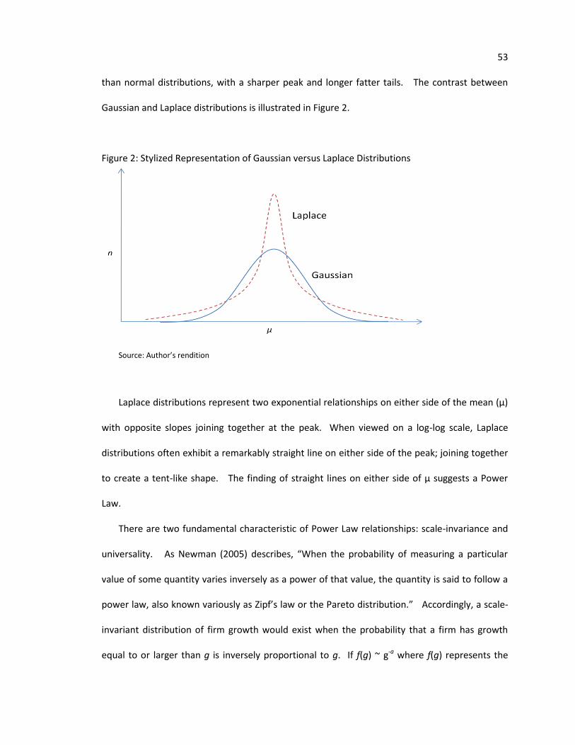
53 than normal distributions, with a sharper peak and longer fatter tails. The contrast between
Gaussian and Laplace distributions is illustrated in Figure 2.
Figure 2: Stylized Representation of Gaussian versus Laplace Distributions
Source: Author’s rendition
Laplace distributions represent two exponential relationships on either side of the mean (µ)
with opposite slopes joining together at the peak. When viewed on a log-log scale, Laplace
distributions often exhibit a remarkably straight line on either side of the peak; joining together
to create a tent-like shape. The finding of straight lines on either side of µ suggests a Power
Law.
There are two fundamental characteristic of Power Law relationships: scale-invariance and
universality. As Newman (2005) describes, “When the probability of measuring a particular
value of some quantity varies inversely as a power of that value, the quantity is said to follow a
power law, also known variously as Zipf’s law or the Pareto distribution.” Accordingly, a scale-
invariant distribution of firm growth would exist when the probability that a firm has growth
equal to or larger than g is inversely proportional to g. If f(g) ~ g-a where f(g) represents the

54 number of firms that have growth of g or greater than g, the exponent a represents the
probability density.
Power Laws were first recognized by Vilfredo Pareto in his study of personal income
distribution in Italian cities more than 100 years ago. He found a scale-invariant distribution
where the number of people having income of x or greater than x was determined by the
exponent a. Pareto went on to measure income distributions at various geographic locations
and scales, including dozens of cities and provinces throughout numerous countries across
Europe, finding similar results.
During the 1930s George Zipf also found scale-invariant relationships in his research on the
frequency of word use in language. He also found that Power Laws held across most languages.
As a result of these early works, the Pareto and Zipf distributions are commonly used to describe
this same Power Law phenomenon.
In more recent years, Power Laws have been found in many probability density distributions
throughout the natural world and even within the field of economics. Newman (2005) explains,
“Power-law distributions occur in an extraordinarily diverse range of phenomena. In addition to city population, the sizes of earthquakes, moon craters, solar flares, computer files and wars, the frequency of words in any human language, the frequency of occurrence of personal names in most cultures, the number of papers scientists write, the number of citations received by papers, the number of hits on web pages, the sales of books, music recordings and almost every other branded commodity, the number of species in biological taxa, people’s annual incomes and a host of other variables all follow power-law distributions.” (page 2).
Power Laws have been found in other economic distributions as well. These include stock
volatility, share volumes traded, and the number of trades per trader (Stanley and Plerou 2001;
Mandelbrot and Hudson 2004). These relationships are demonstrated over different periods of
time, segments of the economy, and different countries, leading to the conclusion that
temporal, industry, or locational variances are not the causal forces driving these distributions.

55 Numerous studies of firm growth have found evidence of Power Laws in the form of straight
lines on the right side of the distribution when charted on a log-log scale. For example, Stanley,
et al. (1996) found Power Laws for U.S. firms using sales and employee data from Compustat
dataset; Axtell (2001) found Power Laws for all tax-paying firms in the US using Compustat and
Census Bureau data; Fu et al. (2005) found Power Laws in the world-wide pharmaceutical
industry using both firm and product sales; Bottazzi and Secchi (2006) found the same
relationship in sales data from Italian manufacturers of various sizes; and Bottazzi et al. (2007)
observed Power Laws in the growth distribution of French manufacturers. In addition, Gatti et
al. (2007) found Power Law distributions among profits for firms located in seven industrialized
countries. These studies generally conclude that distributions are Laplace in nature and are
nearly identical regardless of how size or growth is measured: products or firms; sales or
employees. They also found that Power Laws are demonstrated regardless of which years
define the study period or whether the number of years in the study period increases.
Several scholars have noted that the presence of Power Laws in firm size and growth
distributions has become a benchmark that any new theory of the firm must be able to
adequately explain (Axtell 2001; Stanley and Plerou 2001; Newman 2005). For example, Stanley
et al. (1996) argue that traditional economic theory focuses too heavily on production
technology which varies greatly from product to product. They propose that the development
of a viable theory of the firm must account for commonalities that cross vastly diverse groups of
firms. This change in approach to explaining firm dynamics should focus more on the
‘technology of management’ rather than the ‘technology of production’. They conclude,
“Our central results constitute a test that any accurate theory of the firm must pass. These equations support the possibility that the scaling laws used to describe complex systems comprised of many interacting inanimate particles (as in many physical systems) may be usefully extended to describe complex systems comprised of many interacting animate subsystems (as in economics).” (page 806)

56 Complex systems share the quality of heterogeneous agents that are codependent in their
behavior at some level. This interaction influences their aggregate probability density which is
reflected in Laplace distributions. Scale-invariance leads to similar findings across different
levels of aggregation, behavior measurements, and time periods, which is the hallmark of
universality. As Stanley and Plerou (2001) comment,
“It is becoming clear that almost any system comprised of a large number of interacting units has the potential of displaying power-law behavior. Since economic systems are in fact comprised of a large number of interacting units having the potential of displaying power-law behavior, it is perhaps not unreasonable to examine economic phenomena within the conceptual framework of scaling and universality.”(page 563)
Bottazzi and Secchi (2006) model the Laplace distribution in the growth of Italian firms.
They begin by critiquing Gibrat’s idea that firm growth is independent, even for firms operating
in the same market and geographic space, arguing that because the set of opportunities
available to any given firm is finite within a specific time frame, the seizure of an opportunity by
one firm necessarily reduces the possible number of opportunities available for other firms.
Firms that learn to seize new opportunities are more likely to win new opportunities in the
future, at the expense of their rivals. Consequently, they develop a model that reflects
increasing returns to explain exponential distributions of growth. They write,
“Economies of scale, economies of scope, network externalities and knowledge accumulation are just a few examples of possible economic mechanisms able to generate positive feedbacks within markets, businesses and industries. The overall effect can be described as the emergence of a sort of “attracting force” between the various opportunities that tends to group them in bigger chunks lending to the appearance of two noticeable properties in their unconditional distribution: the presence of a fat tail, which indicates a more likely presence of extremely large number of opportunities assigned to a single firm, and the absence of a natural scale of the underlying process.” (page 14)
Coad (2006) addresses the issue of stochastic processes in Gibrat’s Law of Proportionate
Effects with a study of 10,000 French manufacturing firms. He argues that if serial correlations
exist in annual firm growth, at any point along the distribution, then Gibrat’s strict stochastic

57 assumption is not valid. He argues that early studies of firm growth overlooked Laplace
distributions because of their over-reliance on aggregated data that obscures information on
individual firm performance while employing traditional regression models that dismiss cases of
extreme growth as outliers. He finds autocorrelation in annual growth, which is particularly
strong among larger firms and firms at the far ends of the growth distribution.
Thus, the assumption of increasing returns and the findings of autocorrelation in firm
growth can be viewed as self-reinforcing, and are at the heart of the search for Power Laws in
economics. Durlauf (2005) argues that efforts to find complex systems in economics began as a
search for path dependency, which attempts to explain how shocks can cause permanent
effects on a system. He argues that any suitable model designed to explain a phenomenon such
as firm growth must “adequately respect the purposefulness of individual behavior” within an
environment where agents are interdependent.
A central question of this study is whether this interdependency is best explained by firm-
specific attributes, such as those proposed by the Resource-Based View, or by industry or
location characteristics as strongly advocated by the agglomeration, industrial organization, and
cluster literatures. These questions may be best answered by evaluating the similarities of
Power Law effects across space and industry, as well as by testing the degree of temporal
autocorrelation.
2.3.4 Firm Growth and Regional Growth
Regional employment growth represents the net contributions of individual firms as they
are born, expand, contract, die, and enter or exit a geographical area (Birch 1987; Van Wissen
and Van Dijk 2004; Neumark et al. 2005). Studies evaluating these ‘components of growth’ tend
to agree that the most powerful explanation for differences in regional employment growth,

58 when compared either across space or time, is the magnitude of growth at existing ‘indigenous’
firms. As we shall see, the net effect of all other components of employment change on
regional growth is relatively minor when compared to the expansion of indigenous firms.
The most compelling and widespread evidence shows that a small subset of businesses
achieve exceptional levels of employment growth (re: outliers in the firm growth distribution),
and these firms provide a disproportionate impact on regional employment growth. In fact,
high growth firms appear to be the principle drivers of regional growth differences across space
and time. It is this link between exceptional firm growth and regional employment change that
motivates this dissertation.
David Birch, who compiled his findings into Job Creation in America (1987), was the first
researcher known to use disaggregated firm-level data to inquire into the relationship between
firm growth and regional employment change. Birch (1987) used time-series data that covered
nearly every US firm in existence during the years of 1969 through 1986. He expressed net US
employment change as:
Net Change = (Births - Deaths) + (Expansions - Contractions)
The primary insight offered by Birch (1987) is that regions with high rates of firm births and
a correspondingly high number of growing small firms tend to have faster employment growth
than other regions. While he found that there was little difference in regional rates of firm
contractions and deaths, the variation in firm birth rates and firm growth rates was quite large.
He summarizes: “virtually all of the variation in growth from one place to another is derived
from differences in the rate at which lost jobs are replaced…replacements originate in the
formation of new firms and the growth of existing firms” (p.137).
Birch (1987) focused his writings on the combined effect of birth and expansion of young
firms, arguing that small firms are responsible for almost all net job growth in the economy. He

59 noted that the vast majority of firms in the US are small, with about 90% employing fewer than
20 employees. Other researchers found that less than 5% of start-ups grow to 20 employees
during their first five years after birth (NCE 2001). Another recent paper succinctly explains
“most firms start small, live small, and die small” (Davidsson et al. 2005). Yet, Birch’s instinct to
tout the job generation potential of small firms may have obscured important differences
between the contributions that firm births and firm growth have on regional growth.
More recently, Neumark et al. (2005) used a modified version of Birch’s composition of
employment change to account for firm migration in and out of geographic regions, as
expressed:
Net Change = (Births - Deaths) + (Expansions - Contractions) + (In-Moves - Out-Moves)
Neumark et al. (2005), using a firm-level dataset similar to Birch’s, applied this formula to
California during the 1990s. They find that for every year studied the magnitude of ‘expansions
minus contractions’ was substantially greater than either ‘births minus deaths’ or ‘in-moves
minus out-moves’. In addition, ‘expansions minus contraction’ demonstrated the highest
autocorrelation and was always positive in sign, unlike other components which frequently
changed signs. This indicates that firm expansions are the single most important factor driving
the annual change in employment at the state level. Thus, net expansions are both larger and
more consistent than net births, while the impact of net relocations is negligible.
There is mounting evidence across a range of developed countries that a relatively small
subset of growing firms are responsible for a disproportionate amount of regional net
employment change. Stam (2006) found that a small number of Dutch high-growth firms
contribute far more towards explaining regional employment growth differences than does the
total of firm births. Communities with rapid employment growth tend to possess firms that are

60 experiencing high job growth (Blair and Premus 1987). North and Smallbone (1995, 1996) argue
that most jobs in the UK are created by the most rapidly growing firms.
Contrary to the predictions of agglomeration and cluster theories, firm birth rates and
growth rates are higher in less densely populated counties than in more urban areas of the UK,
as shown in Table 1 (Keeble and Tyler 1995).
Table 1: Urban-Rural Differences in New Firm Formation and Small Business Growth Rates, 1980-90
Region Mean new firm formation rates
Mean small business growth rates
Conurbations 64.4 +8.9
More-urbanized counties 76.7 +14.2
Less-urbanized counties 83.3 +20.5
Rural counties 83.2 +15.7
Source: Keeble and Tyler 1995; p.977
Acs and Malecki (2003) found little regional difference in average firm birth rates when
controlling for Labor Market Area size in the U.S. They write, “There is, on the other hand, a
clear pattern of higher percentages of high-growth firms in smaller LMAs” (p.26). These smaller
LMAs are almost all rural and non-metropolitan communities.
Table 2: Average Firm Births and Percent of High Growth Firms by LMA Size in US.
LMA Size by Population Number of LMAs
Mean Average Firm Birth Rate (1994-1996)
Mean Percentage of High Growth Firms
Less than 50,000 113 3.75 4.73
50,000-99,999 108 3.76 4.50
100,000-200,000 78 3.68 4.38
200,000-500,000 58 3.63 4.21
More than 500,000 37 3.96 3.97
Source: Acs and Malecki 2003, p.26

61
Studies of Dutch firms have found only a weak correlation between firm birth rates and the
location of high-growth firms (Stam 2005; Stam 2006). High-growth firms are more widely
dispersed than firm births, and there is “no clear urban hierarchical logic to the spatial
distribution” of high-growth firms (Stam 2006; p.123).
Dumais et al. (2002) find that areas of high industry concentration (i.e. localization
economies) demonstrate less than a proportional share of firm births and slower average
growth rates of existing firms. On the other hand, firm survival rates are higher in more
concentrated areas. Thus firm births and growth act to decentralize economic activity while
firm deaths, though weaker in strength, contribute to centralization. They write,
“(firm) growth rates are lower in states with a high initial concentration in the industry. New firms are more likely to start away from current geographic centers of the industry, and growth is faster away from those centers, but the risks appear to be higher in the periphery and closures are also higher there.” (p.201). Looking at the spatial distribution of high-growth firms as uncovered in studies spanning
eight countries, Mustar (2002) concluded:
“the occurrence of high-growth firms is roughly in proportion to the overall occurrence of firms across regions, with one or two exceptions per study (which might be due to selection bias). This does not exclude a strong regional concentration of high-growth firms, but such concentration comes along with generally intense economic activity in that region.” (p.25).
Taken together, these studies indicate that firm expansion is responsible for substantially
more regional net employment growth than firm births. They also indicate that neither firm
births nor high growth among firms are disproportionately driven by the spatial density of
populations or firms. Perhaps more importantly, they suggest that high growth firms appear to
be the principle driver of net regional employment change.

62
2.3.5 Firm Growth and Location
For at least half a century human populations and economic activity in much of the United
States have dispersed. These changes are apparent at both the intra-regional and inter-regional
levels (Schmenner 1982; Birch 1987; Essletzbichler 2004). People and businesses have shifted
away from dense urban centers towards the periphery, secondary cities, towns, and rural areas.
Highly agglomerated regions have lost population and employment to less agglomerated
regions. Outside the US, dispersion of manufacturing and total employment has also been acute
in the UK and Northern Europe (Keeble and Tyler 1995; Englestoft et al. 2006).
Changes in the location of US manufacturing and workers has been documented and
studied by many scholars (for example Schmennar 1980, and Birch 1987). Perhaps nowhere
has dispersion been more apparent than in the decline of dense manufacturing ‘Rustbelt’ areas
of the northeastern US and the corresponding rapid growth of many lower-density ‘Sunbelt’
areas in the US south and west. Between 1967 and 1982 the New England, Mid-Atlantic, and
East North Central regions lost 2 million manufacturing jobs while states in the south and west
gained 1.5 million (Essletzbichler 2004). The overall decline in geographic concentration of
economic activity continued into the 1980s throughout the US (Dumais, Ellison et al. 2002),
along with rising concerns about perceived problems associated with ‘urban sprawl’. During
the 1990’s the “massive de-urbanization of manufacturing in American cities” was still
proceeding at a rapid pace as production shifted to “lower-density, less expensive areas”
(Glaeser and Shapiro 2003).
Bram and Anderson (2001) evaluated the 51% decline in manufacturing employment in the
New York-New Jersey region from 1969 through 1999, a time when national losses in
manufacturing employment were less than 9%. This region lost more manufacturing jobs over
this time-span than any other area of the country. They find that the spatial density of

63 manufacturing (average manufacturing jobs per square mile) declined steadily in the ten states
with the highest density while it constantly rose for the ten states with the lowest density.
During this same time, the average US manufacturing density remained relatively unchanged.
Thus, it is not simply true that manufacturing ‘disappeared’ in the US during this time. Rather,
the dominant trend has been the shift of production from regions of high agglomeration to
regions of low agglomeration.
Economic dispersion is also evident in the large-scale shift of US manufacturing from urban
areas to rural areas. From 1967 to 1997 manufacturing employment in metropolitan counties
declined by 1.7 million while, during the same period, rural counties added 930,000 new jobs
(Essletzbichler 2004). During this time rural counties and small towns enjoyed both higher levels
of job creation and lower levels of job destruction than urban counties and large metropolitan
areas. Since the 1980’s rural counties, on average, enjoyed higher manufacturing employment
growth than urban counties in every region of the country.
Dispersion is also evident in household migration and ‘urban sprawl’. In Midwestern states
and the Great Lakes region, the percentage of residents located in the central city of the largest
ten metropolitan areas consistently declined between 1970 and 2000 (Crary et al. 2003). For
example, the percentage of inner city residents in Detroit fell from 33.7% in 1970 to 21.4% in
2000, while Chicago’s inner city proportion fell from 47.4% to 35%. Population decentralization
throughout the country continues to be the “dominant overall trend” as workers and their
families flee cities for suburbs and smaller towns (Berube 2003).
These trends raise very challenging questions for cluster theory. Why would rational
business owners and workers choose to disperse when both agglomeration and cluster theories
argue that positive spatial externalities found in concentrated areas raise productivity and living
standards? Can these population and production shifts be attributed simply to rising costs and

64 negative congestion externalities in urban areas? Alternatively, could decentralized areas be
more appealing in their own right, aside from these other effects? Cluster theory simply fails to
address why many areas of the developed world have witnessed a mass migration of businesses
and workers away from ‘clusters’ and other densely agglomerated areas over the past four
decades.
Early scholars of agglomeration theory recognized ‘deglomeration forces’ as the rising costs
of land and labor caused by increasing spatial concentration of economic activity (Weber 1929).
In recent years scholars have articulated a wider range of dispersion forces which include both
pecuniary (re: price) effects such as Weberian rising wages and rents, as well as non-pecuniary
effects that are transferred outside the pricing system (re: negative externalities of
concentration). These negative externalities can include the congestion of public infrastructure,
environmental pollution, greater propensity of union activity, and space limitations for
expansion (Edmiston 2004). Both cost effects and negative externalities are thought to
counteract, at least in part, the positive externalities of agglomeration. In this view, the
dispersion of economic activity is likely if the costs (both pecuniary and non-pecuniary) of
concentration dominate the benefits.
Some scholars interpret empirical evidence as support for this cost/benefit view of location.
For example, Wallace and Walls (2004) evaluated the California computer manufacturing
industry using firm-level data to measure whether the benefits from agglomeration overcome
increased costs. They find that “the wage increase or congestion effects of proximity to large
numbers of competitors’ employees in computer manufacturing outweigh the potential
advantages of these localization effects through increased labor market availability” (p.24).
Scholars see similar forces at work in the Indian manufacturing industry (Lall et al. 2001).

65
Yet the Weberian notion that firms choose decentralized locations when ‘deglomeration’
forces overpower agglomeration forces fails to explore alternative explanations. The
cost/benefit framework implies that firms actively engage in location decision-making. Yet, the
benefits of agglomeration may be negligible or inconsequential for many firms, leading some to
pursue the default expansion mode of in-situ growth without undergoing an active evaluation of
alternatives. They thus engage in satisficing behavior, avoiding information search costs.
Perhaps more importantly, dispersion may enhance a firm’s competitive advantage in ways
hinted by Penrose (1995) but ignored entirely by Porter (1990, 2000a, 2000b).
Penrose (1995) believes that managers make decisions within the constraints of bounded
rationality. As such, location choice may be as much determined by objective characteristics of
the environment as it is by perception and belief. Studies of site preferences find that firms
overwhelmingly prefer locations they are previously familiar with, particularly within their local
region (Meester 2000). Such behavior can reduce uncertainty when faced with unfamiliar
decisions and substantial operational changes.
Firms overwhelmingly choose on-site expansions as their preferred method to add capacity
(Schmenner 1980). This is usually the least expensive alternative, involving the least amount of
time to plan and execute. It is least disruptive to current operations and is favored by plant and
division managers because it allows them to spread overhead across a larger number of units
(Schmenner 1982). Fortune 500 companies interviewed by Schmenner also mentioned that a
key motivation for on-site expansion was ‘keeping management together’ (1982; p.91). This
seems to match Penrose’s argument that inherited managers are both the primary growth
enabler and limitation.
Start-ups overwhelmingly occur near a founder’s residence. Founders are typically
preoccupied with practical issues related to starting their enterprise – financing, product

66 development, sales, hiring, etc. – rather than engaging in an extensive site search (Pellenbarg
2005). Thus, with start-ups and in-situ growth, expansion increases employment without
necessarily making a firm’s location a strategic planning issue (Walker and Greenstreet 1990).
Location is essentially determined by default to path-dependency. If a firm survives the start-up
period and begins to rapidly grow, at some point they are likely to move to a new facility. At
that point location decision-making begins; often integrated into the firm’s strategic planning
process. Only relocation and branching, rather than in-situ expansion, requires an active site
search, and is thus a form of revealed preference (Pen 2000).
Taste heterogeneity for different types and levels of amenities can also act as a force for
population dispersion (Tabuchi and Thisse 2001). If locations are considered heterogeneous in
their amenities and humans are considered heterogeneous in their preferences, human
populations will disperse. The migration of entrepreneurs seems to play a large role in
determining the spatial pattern of firm births and subsequent expansions (Markusen 2006;
Markusen and Johnson 2006). In the UK, far more founders of rural firms moved prior to
starting their companies than urban firms (Keeble and Tyler 1995). More urban firms were born
in the place where they reside than those in rural areas, while more urban firms move to rural
areas than vice versa. In fact, one-fifth of rural firm founders reported to have moved in order
to establish their firms. Many founders relocate to rural from urban areas for personal
preference reasons, often seeking a better ‘quality of life’. This trend has been observed in the
US as well (Beyers and Lindahl 1996; Henderson 2002).
A more recent study confirmed that more than half of new firms in rural England are
founded by in-bound migrants (Kalantaridis and Bika 2006). These entrepreneurs rely less upon
local suppliers and markets and more upon pre-existing and distant networks outside their new
locations. Other studies of successful firms have also found that their networks are typically

67 non-local rather than local (Acs and Malecki 2003). They write, “The level of innovativeness and
competitiveness of firms in rural areas, or any area, depends not only on the degree to which
firms are tied to local networks of suppliers but also to external markets” (p.22).
Thus, some entrepreneurs - including those that create high-growth firms - may simply like a
place and what it has to offer, move there, and then establish and grow their business. Some
may prefer non-urban amenities or some intrinsic hedonic value of less populated areas. This
fact is conveniently overlooked by scholars that argue that there is an innate and rational
tendency for ‘creative’ individuals, including entrepreneurs, to migrate to urban areas (Florida
2002).
Wojan and Pulver (1995) argue that most location scholars dismiss the prospects of rural
areas, taking for granted that firms will only locate in rural areas during the end of their life-
cycles (see Vernon 1966). This literature tends to treat rural areas as homogeneous and ignores
indications that some locations may be more competitive than others. “Unfortunately, little
attempt has been made to explain why the same industry might prosper in a number of
different types of places or why places with similar endowments do not contain similar
collections of industry” (Wojan and Pulver 1995; p.5).
Cluster theory assumes that co-located firms learn from others in their environment
through knowledge spillovers and that these inputs are needed for innovation. This implies that
firms in areas with little spillover opportunities are unlikely to be as innovative and thus under-
perform when compared to competitors in more agglomerated areas. Thus, agglomeration
literature dismisses the growth potential of remote firms because it assumes that spillovers are
necessary for innovation (North and Smallbone 2000).
Regional science literature generally argues that firms in non-urban areas suffer from a lack
of external resources such as capital, qualified labor, suppliers, infrastructure, as well as low

68 levels of local demand and growth (Birley and Westhead 1990). These deficiencies are expected
to result in lower rates of innovation, supply bottlenecks, pursuit of inefficient vertical
integration strategies, and less success in specialized market niches. These arguments are
found in Porter’s writings as well (1990, 2000a, 2000b).
British researchers have extensively studied the strategies used by rural small and medium
size enterprises (SMEs) to adapt to their environments (Smallbone et al. 1999). They find that
the most common characteristics of remote SMEs are “proactive product and market
development to overcome the limited size and scope of local markets; a labour-intensive
development path to exploit the potential advantages of remote rural labor markets; and a
relatively low level of subcontracting-out of production activities” (p.109). They argue that
these adaptive strategies enable remote SMEs to survive and thrive despite environmental
constraints.
There is also ample empirical evidence that high-growth rural firms are just as innovative as
their urban counterparts (Vaessen and Keeble 1995). Yet high growth is not only associated
with ‘innovation’ but also with expansion into distant markets. Among rural SMEs, there is a
statistically significant association between the development of innovative products or services
and the development of non-local markets (North and Smallbone 2000). For example, firms
with higher growth and profitability are more likely to become exporters (Bernard and Jensen
1999). Exporters tend to produce twice as much output as non-exporters, demonstrate higher
productivity, and pay higher wages than non-exporters. Exporting also tends to increase firm
survivability. It may be that large local markets are not as important for firm-level growth as
implied by agglomeration theory.
The average profits of SMEs in rural and urban areas are not statistically different from one
another, although urban firms do not create as many new jobs as their rural counterparts

69 (Combes and Duranton 2001). Among small and medium-size firms in the UK between 1979 and
1990, those located in remote rural areas generated far more employment on average than did
firms in outer metropolitan areas or central London (North and Smallbone 1995). This may
reflect a self-sufficiency of remotely growing firms.
Expansion constraints reported by urban and rural firms seem to differ (Keeble and Tyler
1995). Perhaps as expected, rural firms report more problems with recruiting experienced staff
as well as dissatisfaction with communication and transportation infrastructure. Rural firms
report less difficulty expanding existing facilities than urban firms, yet they also complain that
there are fewer buildings available for local relocations (Keeble and Tyler 1995).
However, firms in inner-London report more constraints to expansion than periphery or
rural firms, especially regarding labor (North and Smallbone 1995) . Three times as many UK
inner-city firms reported problems with employees regarding issues such as worker age,
retention, and worker motivation. Perhaps as a consequence, London firms were more active
in sub-contracting parts of production to suppliers. “SMEs in inner London have more incentive
to seek ways to achieve growth (or even survival) which avoid the constraining effects of labor
than their rural counterparts” (p.1527). These findings imply that some firms choose rural
areas to avoid growth constraints imposed by urban environments.
Stam (2005) found that Dutch high-growth high-technology firms were commonly found in
rural and peripheral areas. He concludes: “Firms that face greater environmental constraints
than their counterparts in core regions as they grow, may in fact adopt a more pro-active
attitude, via manipulation, immunization and adaptation mechanisms, which in turn renders
them more competitive in wider markets” (p.125). Evidence from the UK suggests that firms
located in rural areas develop innovative ways to over-come local resource constraints
(Smallbone et al. 1999; North and Smallbone 2000). For example, rural firms are more likely to

70 pursue internal training programs in order to overcome shortages in skilled labor (Vaessen and
Keeble 1995). Environmental adaptation can potentially make these firms more competitive
than firms located in relatively resource-rich areas.
Recent research in the entrepreneurship literature indicates that the entrepreneurial
orientation (EO) of a firm may allow it to adapt to adverse constraints imposed by
environmental and resource constraints (Wiklund and Shepherd 2005). EO refers to the way
firms make decisions, combining traits such as innovation, proactive attitude, and risk-taking.
These researchers compared the performance of firms in environments with various levels of
access to financial resources and market dynamism. They found, “while performance increases
with increasing EO for all configurations, it increases at a faster rate for those in a stable
environment with little access to financial capital than for all other combinations of access to
financial capital and environmental dynamism” (p.84). A strong EO can thus act as a mechanism
for differentiation, similar to the old saying that ‘necessity is the mother of invention’ (Wiklund
and Shepherd 2005).
An evaluation of the patterns of advanced technology adoption rates by firms in different
size communities found that firms within urban areas tended to rely upon external expertise
whereas firms in rural areas developed their own in-house talent (Forman et al. 2005).
Agglomeration seems to benefit smaller single-establishment firms more as they substitute
external for internal resources. As firms grow, they tend to develop more internal resources
and have less need for external resources found in cities. This may reinforce a tendency to
relocate to less agglomerated areas as they grow. Other scholars argue that as managers in
rural areas adapt to the resource limitations of their environment they may become more self-
sufficient and less dependent upon external knowledge spillovers or supplier relationships

71 (North and Smallbone 2000). Thus, agglomeration may benefit weaker or younger firms more
than older or more adaptive and innovative firms.
A German study found a slightly negative correlation between technology intensiveness of
an industry and its propensity to agglomerate (Alecke and Alsleben 2004). Industries considered
either high- and medium-technology intensive are agglomerated about average or less than
average when compared with all German industries. Alsleben (2005) also found that firms in
industries characterized by strong competition tend to be less agglomerated.
A recent study of clustering among Dutch firms in the information and communications
industries found that agglomeration effects are not a strong determinant of firm growth (Van
Oort and Stam 2005). These researchers note “knowledge, as an input for growth of incumbent
firms is associated with more endogenous (firm internal) learning aspects, reflected by a
significant correlation with R&D-investment” (p.1). They also note that the level of local
competition within the cluster has a positive effect on firm-birth but a negative effect on firm
growth.
Shaver and Flyer (2000) point out that if firms are considered heterogeneous, then they will
benefit differently from agglomeration. Hence, some firms will benefit from knowledge
spillovers at the expense of others. Firms with the ‘best’ knowledge may wish to avoid
clustering with competitors, while those with ‘poor’ knowledge would more strongly seek to
cluster. This would potentially result in spatial adverse selection, where clusters become
concentrations of mediocrity once superior firms depart.
One of the primary mechanism that facilitates knowledge spillovers is labor turnover which
often takes the form of ‘labor poaching’ when, for example, one firm hires employees with
proprietary knowledge from a competitor (Alsleben 2005). Labor poaching is a way that some
firms can free-ride from the research and development efforts of others. Firms that aggressively

72 invest in R&D have an incentive to protect themselves from loosing valuable rent-generating
knowledge. To do so they can increase wages to make it harder for rivals to poach (Combes and
Duranton 2001; Alsleben 2005). A recent survey found that agglomerated firms were much
more concerned with the risk of ‘head-hunting’ then were dispersed firms (Lublinski 2003).
Perhaps dispersion can thus be considered an isolation mechanism in the spirit of Penrose
(1995).
The studies reviewed here make it clear that the relationship between dense locations and
firm growth is not as powerful as implied by agglomeration or cluster theory. Non-dense
locations may be preferred by rational decision makers, for reasons of taste, path-dependencies,
competitive and/or cost advantages, or other factors not considered here. However, this
evidence does give strong rationale to test the degree to which location influences firm-level
growth as predicted by much of the regional science and cluster literature.
2.3.6 Firm Growth and Industry
As reviewed above, there are plenty of rapidly growing firms located in rural areas that
compete in the same industry segments as urban firms (Henderson 2002). In addition,
numerous studies have shown that firms with high levels of employment growth are found in all
industry sectors and are not over-represented in industries considered as ‘high-technology’ or
‘knowledge-intensive’ (Birch 1987; Autio et al. 2000; NCE 2001; Stam 2005). As Davis,
Haltiwanger, and Schub (1998) observe, “knowing the industry to which an establishment
belongs provides very little information about its job creation or destruction”. These
counterfactual examples clearly imply that the link between clusters and firm-level growth may
not be as strong as described by Porter.

73
There has been a long running debate between scholars about whether firm performance is
best explained by industry-effects as advanced by IO literature and Porter, or by firm-effects as
argued by Penrose and RBV researchers (Porter 1981; Rumelt 1991; McGahan and Porter 1997;
Mauri and Michaels 1998; Hawawini et al. 2003; Ruefli and Wiggins 2003; Hawawini et al. 2005;
Chen and Lin 2006). Empirical studies have measured the dependent variable, firm
performance, primarily in terms of accounting profits, return-on-investment, or return-on-
assets. Industry-effects are measured as the industry association of the firm.
Rumelt (1991) was the first scholar to study firm performance using time-series data. He
found that firm-effects were six times stronger than industry-effects in explaining the variation
of profits among firms in the same industry. He concluded:
“The ‘classic focus on industry analysis’ is mistaken because these industries are too heterogeneous to support classical theory. It is also mistaken because the most important impediments to the equilibrium of long-term rates of return are not associated with industry, but with the unique endowments, positions, and strategies of individual businesses.” (p.168). The dominance of firm-effects over industry-effects has been confirmed by other
researchers (Hawawini et al. 2003; Chen and Lin 2006) and has been grudgingly acknowledged
by Porter himself (McGahan and Porter 1997). It is now generally accepted that firm-effects
explain most of the variance in long-term performance between firms (Geroski 1998; Hoopes et
al. 2003).
Hawawini et. al. (2003) focused their attention on the role of outliers in time-series
performance data, arguing that important firm-specific information is often deleted or obscured
through data aggregation, particularly when researchers use Ordinary Least Squares models.
They write:
“We find that a significant proportion of the absolute estimates of the variance of firm factors is due to the presence of a few exceptional firms in any given industry. In other words, only for a few dominant value creators (leaders) and destroyers (losers) do firm-

74
specific assets seem to matter significantly more than industry factors. For most other firms, i.e. for those that are not notable leaders or losers in their industry, however, the industry effects turn out to be more important for performance than firm-specific factors.” (p.1) They interpret their findings to indicate that industry-effects have the largest impact on the
‘also-rans’ in an industry but not on those firms able to achieve and maintain exceptional
performance (p.14). They later write that there is evidence in their data that economic
performance may be ‘sticky’ in that superior performance seems to persist in a significant
number of companies across most industries (Hawawini et al. 2005).
These results suggest that a firm’s unique attributes have a much greater influence on its
ability to achieve and sustain growth than does its industry affiliation. Birch (1987) reminds us
that the concept of ‘industry’ is a social construct. He wryly observed, “No one reading this
book works for an industry...rather jobs are supplied by a specific company or, perhaps, a
division of a company, or by themselves” (p.1).

CHAPTER 3: INQUIRY DESIGN This dissertation seeks a deeper insight into the phenomenon of firm growth and its
relationship to net employment change within in a region over time. The inquiry is both
empirically based and theory driven, using deductive reasoning to guide the exploratory
inductive analysis. For empirical grounding, it uses establishment-level time-series data to track
the characteristics and performance of a cohort of all known businesses in the Commonwealth
of Pennsylvania over the 1997-2007 period. For theoretical guidance, it is informed by the
works of Gibrat, Porter, and Penrose, among other scholars working in the fields of firm growth,
theory of the firm, cluster theory, agglomeration theory, and industrial organization.
3.1 Research Questions
As discussed previously, both Porter’s cluster theory and Penrose’s RBV rely upon the
fundamental premise that firm-level growth is not entirely random for all businesses. Both
scholars believe that some firms are better endowed than others with either internal (RBV) or
external (cluster theory) attributes that provide them with competitive advantages over rivals.
The presence of these advantages should be revealed by superior growth and survival when
compared with less endowed firms.
Gibrat, in contrast, argues that firm growth is stochastic, meaning that there should be no
lasting systematic performance differences between firms. Thus, Gibrat’s Law of Proportionate
Effect is the null hypothesis to both cluster theory and RBV. This study tests for stochastic firm
growth in two ways: by evaluating whether the distribution of firm growth exhibits tendencies

76 of a Power Law, and by checking if past growth has any ability to predict future firm growth or
survival. The presence of a Power Law would indicate that a subset of firms systematically
accumulates a disproportionate amount of growth, suggesting increasing returns to their
endowments9. However, this alone does not inform us as to which endowments are most likely
to generate performance differences.
Consequently, this study proceeds to test the relative strengths of endowments related to
firm-specific characteristics related to RBV, as well as industry, policy, and location
characteristics representing cluster theory and its associated literatures. These tests compare
the abilities of these respective characteristics to explain past growth and to predict future
growth and survival.
The model used to describe firm growth can be expressed as:
G = f (F, I, C, L, P)
where the dependent variable G is a measure of firm growth, and is a function of independent
variables: F firm characteristics; I, industry sector affiliation; C, cluster policy; L, location
attributes; and P, past performance. In a slightly modified form, S is substituted for G with the
same right-hand variables, where S is survival of the firm to a specific point in time10, whereas:
S = f (F, I, C, L, P)
This inquiry is guided by the following research questions:
Q1: What is the relative strength of firm (F), industry (I), cluster policy (C), or location (L) characteristics to explain firm employment growth,
a: over a ten year period (1997-2007)?
b: over five year pre-recession and post-recession periods (1997-2002 and 2002-2007)?
9 Tests for Power Law in the growth distribution are described and presented in Section 5.1.
10 Tests of this model are presented in Section 5.2.
77 Q2: How do the explanatory strengths of the independent variables F, I, C, and L differ,
a: at different points along the growth distribution (re: from negative to high growth)?
b: by the way employment growth is measured (re: absolute, relative, or sustained)?
Q3: How well do F, I, C, L, and past growth, P, predict,
a: future firm growth (re: growth in 1997-2002 vs. growth in 2002-2007)?
b: future firm survival? (re: growth in 1997-2002 vs. survival through 2007)?
The hypotheses tested in this study are informed by the literature review. Because the
intent of the analysis is to compare alternative theories related to firm growth, we will
generously anticipate that there is at least some validity in both RBV and cluster theory.
Therefore,
H1: Firm growth follows a Power Law, where a subset of establishments accumulates a disproportionate amount of growth over time.
H2: Firm (F), industry (I), cluster policy (C), and location (L) all have significant influence on
explaining establishment-level growth in a past period. H3: Firm (F), industry (I), cluster policy (C), location (L), and past growth (P) all have
significant influence on predicting establishment-level growth and survival in a future period.
The expected relationships between each independent and dependent variable is discussed in
Section 3.6.
3.2 Dataset
This analysis primarily relies upon the National Establishment Time Series database (NETS)
which contains information on all known establishments located in the Commonwealth of
Pennsylvania between 1997 and 2007. NETS was compiled using Dun and Bradstreet’s (D&B’s)
DMI records on an annual basis. Dun’s Market Identifier (DMI) files contain information on

78 more than 100 variables related to firm demographics (e.g. age, location, industry, ownership),
operations (e.g. corporate structure, secondary and tertiary SICs, relocations), as well as
performance (e.g. sales, employees).
D&B, as part of its global business credit rating service, tracks more than 52 million
businesses in more than 200 countries each year. About 11 million of these files are updated
annually. The updates are based on information collected from more than 100 million
telephone calls made each year from four call centers, as well as from legal and bankruptcy
filings, press reports, utilities, government and U.S. Postal Service records, and payment and
collection activities (Acs et al. 2008)11. D&B uses a variety of proprietary data cleaning
processes to cross-check and standardize the data in order to improve reliability. These
processes have been greatly improved over the past two decades and are now augmented by
further screening by Walls & Associates, a boutique data consulting firm who D&B licenses the
use of the DMI files.
D&B assigns a unique DUNS (Data Universal Number System) number to every
establishment. It then reports annual operating information for each of these businesses,
retiring the DUNS number once an establishment dies. The DUNS allows D&B to link the
employment, location, and operating profiles of companies across their parent company
organizations on an annual basis.
Walls & Associates, under contract with D&B, obtains annual updates for all DMI files. It
then uses the DUNS to create a time-series for each company by linking these annual files based
on the DUNS numbers. Walls & Associates then applies a proprietary screening system to
eliminate duplicates and identify reporting anomalies in the records. If a file contains suspicious
information, Walls & Associates cross-checks the information with previous annual records and
11
See also hhtp://mddi.dnb.com/mddi/story.aspx.

79 will then adjust the data based on their own estimate, or eliminate the record. A variable
created by Walls & Associates identifies each file that has been altered and reports how the
change was made.
Birch (1987), a pioneer researcher in the field of firm-level growth, used a dataset similar to
NETS which he compiled himself using D&B records on a bi-annual basis between 1969 and
1986. There are only a few published articles which use NETS (Wallace and Walls 2004;
Neumark, Zhang et al. 2005). These researchers express confidence that NETS is suitable for
studies of both firm-level employment changes and regional employment growth and
agglomeration.
Davis et al. (1998) provide the harshest critique of the use of DMI data by Birch and the U.S.
Small Business Administration (SBA). They argue that because DMI is prepared for commercial
purposes rather than as a tool for statistical analysis, it is an “unsuitable database” for regional
employment analysis (p.70).
There are two key problems with DMI as suggested by Davis, et al (1998) and several
researchers they cite. First, they point out that there is a large discrepancy in the total U.S.
employment figures cited by DMI files when compared with statistics published by the Bureau
of Labor Statistics (BLS) or the Bureau of Census. In particular, they identify what they believe
are “most serious data problems in the DMI files involving younger and smaller businesses”
(p71), suggesting that any conclusions based on DMI files should be “interpreted with special
caution”.
Secondly, Davis et al. (1998) argue that DMI files inadequately account for company births
and deaths. This is particularly troublesome, they believe, in cases where there are mass layoffs
or other large-scale changes in total employment. They conclude that “DMI files are unsuitable
for generating job creation and destruction figures” (p71).

80 To address the first criticism – that DMI files under-report firm births – Acs et al. (2008)
made a comparison of NETS with the Business Information Tracking System (BITS) database that
is jointly prepared by Census Bureau and SBA. BITS is designed to track all private sector firms
over the 1990 to 2006 period. They began by ranking US metropolitan areas based on three
categories of employment size including start-ups using results from the BITS and DMI. They
report that, although the methodologies used by the datasets differ, the MSA rankings are
essentially unchanged.
Acs et al. (2008) also dispute the claim that federal statistics are better at reporting very
small and start-up businesses. They say that all datasets have problems detecting part-time sole
proprietorships, such as part-time waitresses or consultants. DMI, they say, reports
approximately 5 million of these while BLS does not report any. When DMI files were compared
with BLS’s Employment and Earnings Series in July of 2007, BLS reported 138.1 million workers
compared with DMI’s 142.9 million – a difference of 5 million that may be accounted for by the
part-time proprietors tracked by DMI but missed by BLS.
In fact, Acs et all (2008) show that BLS ignores a total of 18 million proprietorships when
counting full-time sole employee businesses, while DMI ignores 13 million. They argue that
both DMI files and Labor Department have weak coverage of firm births because it can take up
to three or more years for these firms to be discovered, identified, and recorded as valid new
businesses.
One of the primary advantages of DMI files over federally-generated statistics is that
government data releases are limited by legal requirements that ensure confidentiality of each
business entity. Most government statistics on business establishments are collected from
ES202 unemployment compensation reports. Consequently, it is not possible to use BLS data to
track changes at the establishment level in key operational characteristics such as employment,

81 location, or ownership. In contrast, DMI data is submitted voluntarily and there are few legal
limitations to the use of the data by researchers and scholars.
Acs, et al (2008) address one of the central critiques of the DMI files: whether data created
by private companies for commercial purposes is suitable for use by academic researchers.
They conclude, “Although D&B does not collect data for scholarly research, it does have an
incentive to ensure its accuracy, as inaccuracies would jeopardize D&B’s core business and
might result in lawsuits” (p17). Unlike federal statistics, NETS allows researchers to fully
decompose the source of employment change into its components: births, deaths, expansions,
contractions, and relocations into and out of a U.S. region.
While there are differences in the employment figures obtained from BLS and DMI datasets,
there are also frequent and substantial discrepancies across federally-generated statistics.
Neumark et al (2005) point out that two of the main sources of overall employment statistics in
the U.S. economy - the Current Population Survey (CPS) and the Current Employment Statistics
(CES) payroll survey – routinely demonstrate ‘large and persistent’ differences and often report
different trends. They also point out that the payroll surveys entirely exclude the self-employed,
casting some doubt on its accuracy.
There have been large improvements in the methodology used to gather, screen, and clean
establishment-level data since Birch’s dataset was developed in the 1980s (Neumark et al 2005).
For example, in 1991 the regional Bell telephone companies were allowed for the first time to
sell the information they collected. This enabled D&B to greatly increase the number of
establishments they reported, simply by using the Yellow Pages to identify new business units.
Neumark et al (2005) compared the employment levels of NETS for the State of California
with several federally-produced datasets including the Quarterly Census of Employment and
Wages (QCEW) and the Current Employment Statistics survey (CES), and the Size of Business

82 data (SOB). They found a correlation of 0.994 in the total level of employment between NETS
and QCEW; a 0.948 correlation between NETS and CES; and a 0.817 correlation between NETS
and SOB. In fact, NETS reports 184% more employment in establishments in the 1-4 employee
size range than SOB, and 29% more in the 5-9 employee size range. They also report NETS had
total employment of 17-22% higher than QCEW for the various size ranges.
Neumark et al. (2005) do conclude that there is a “good deal of rounding of employment
levels in NETS”. They find that there is a concentration of employment numbers that are
divisible by 5, 10, 100, and so on. They believe that numbers are rounded to the closest ‘salient
number’ and that, on an aggregated level, they are unlikely to be biased appreciably because
the variation will be randomly higher or lower. They conclude: “It does, however, mean that
employment change is “sticky” and that our estimates likely underreport the frequency with
which establishments change their levels of employment, thereby underestimating the degree
of employment change caused by establishment expansion and contraction” (p.17).
Another source of ‘stickiness’ is due to the fact that not every establishment is updated each
year. For example, between 1993 and 2002 between half and three-fourths of each year’s
employment levels is based on actual data. The other figures are estimated by either D&B or
Walls & Associates using time-series information. They conclude that NETS compares less
favorably with other data sources when researchers are evaluating short-term employment
changes. However, Neumark et al. (2005) believe that this problem is mitigated if comparisons
are made with at least a three-year interval. “The implication of these findings is that the NETS
database should not be used for measuring very short-term employment changes, but is more
useful for measuring employment changes over periods of a few years or more.” P19.
In addition to the establishment-level data contained in NETS, this study also uses
information from US national and state agencies. This includes demographic data from the US

83 Census Bureau and Department of Agriculture, industry growth data from the Bureau of Labor
Statistics, and policy information from Pennsylvania’s Department of Community and Economic
Development.
Neumark et al. (2005) comment that there is no obvious ‘gold standard’ for firm-level data
because each dataset has its own strengths and weaknesses, as discussed above. However, the
NETS dataset appears to be the only available source of information that will allow the
establishment-level analysis needed to adequately address the research questions posed by this
inquiry.
3.3 Research Design
There has been considerable discussion in the literature regarding the most appropriate
methodologies to use in studies of firm-level growth, particularly related to datasets and
analytical tools. Scholars have generally concluded that growth studies should be longitudinal in
design; tracking firm performance over time. There has also been increased recognition that
firm-level growth is not normally distributed, posing serious problems for traditional regression
analysis. Therefore, researchers must carefully choose appropriate methods that can
accommodate outliers such as high-growth firms.
Several leading scholars in the field of firm growth study believe that the preferred method
for evaluating firm-level growth is to track a cohort of firms over time (Davidsson et al. 2005;
Garnesey et al. 2006). Davidsson and Wiklund (1999) write, “Growth is a process and therefore
designs must be longitudinal” (p.1). Cross-sectional studies disregard problems with
autocorrelation which can bias analytical results (Walker and Greenstreet 1990). There is a
trade-off, however, between using cohort tracking versus a cross-sectional design. Cohort
analysis creates ‘survivor bias’ because it eliminates those firms that died during the study
84 period (Garnesey, Stam et al. 2006). This limitation is considered acceptable to these
researchers, however, when weighed against the benefits of using time-series data to measure a
temporal phenomenon like growth.
Most longitudinal studies track cohorts of firms for four to ten years (Delmar and Davidsson
1998; Mustar 2002). As the tracking period increases, more firms are lost to death and out-
migration, increasing the problem of survivor bias. However, longer tracking periods help
overcome problems with ‘sticky’ performance data which often result when information is self-
reported by firms (Neumark et al. 2005). Using longer study periods also improves
measurement of growth sustainability as it increases the number of observations and thus
strengthens analytical validity (King et al. 1994).
The dataset used in this study is well suited to accommodate longitudinal analysis. It tracks
a cohort of establishments from 1997 through the following ten years, until the end of 2007.
The vast majority of firms never grow beyond a few employees. Consequently, studies of firm
growth often limit their analyses to firms that have grown to at least 20 employees by the
beginning or end of the tracking period (Delmar and Davidsson 1998; NCE 2001; Delmar et al.
2003; Stam 2005). It is also common to limit the analysis of firm growth to one industry sector,
primarily manufacturing, often due to data availability. Such restrictions, by industry or size,
have the benefit of increasing the explanatory power of the analysis in terms of internal validity.
However, they suffer by reducing external validity when the breadth of inquiry is truncated,
which effectively compromises the ability of theorists to generalize the findings.
Most studies of firm growth limit their analysis to independent firms (Stam 2005). In fact,
only 4% of US firms have more than one establishment (Acs and Malecki 2003). Some studies
differentiate between organic growth and growth via acquisition (Delmar and Davidsson 1998).
Recent studies have shown that small and young firms are much more likely to grow organically

85 than are larger and older firms (Davidsson et al. 2005). Failing to control for these important
differences can lead to specification errors and can bias the results of analyses (Walker and
Greenstreet 1990).
There are numerous ways firm growth can be measured, such as changes in employment,
sales, market-share, capitalization, or other variables. However, the most appropriate firm
growth measurement is the one that best matches the theoretical questions posed by the
researcher (Davidsson et al. 2005). The use of employment growth can be an appropriate
measure when researching within the Resource-Based View or for topics related to public
policies. Delmar et al. (2003) write,
“If firms are viewed as bundles of resources, a growth analysis ought to focus on the accumulation of resources, such as employees. Furthermore, when a more macro-oriented interest in job creation is the rationale for the study, measuring growth in employment seems the natural choice” (p.194) However, using employment growth alone does narrow the measurement of firm
performance. Penrose (1995) recognizes the trade-offs inherent in using any single measure of
firm growth, “A measure of plant size in terms of employment will understate the effects of
increasing mechanization, while a measure in terms of capital equipment will distort comparison
of plant sizes between regions where the relative prices of labour and capital are different, or
between periods of time in which the ‘utilization’ of plant has changed” (p.92).
Despite its drawbacks, employment growth remains the preferred measure of firm growth.
Employment growth is not as sensitive to inflation or currency changes when compared with
sales growth or other financial measures (Delmar et al. 2003). In addition, scholars have found a
high correlation between growth measures over time (Hart 2000). For example, the relationship
between firm number, employees, payroll, and sales are correlated at .88 or better (Shaver and

86 Flyer 2000). There also seems to be a correlation between growth and age generally, although
not necessarily between high-growth and age (Mustar 2002).
There are also trade-offs related to the specific choice of employment growth
measurements. Davidsson and Wiklund (1999) recommend using a compound measure of
growth by combining absolute and relative employment growth. This acts to balance the
observation that initial firm size will bias the measurement of absolute and relative growth in
longitudinal studies12. As a pioneer in this field of study, Birch (1987) used a ‘Growth Index’: a
composite that measures employment growth by simply multiplying absolute growth by the rate
of growth.
Perhaps surprisingly, neither the work by Birch (1987) nor any other research reviewed for
this study incorporated measurements of sustainability into their analyses. Yet, the issue of
sustainability is crucial for understanding the dynamics of firm-growth, especially if growth is not
found to be entirely stochastic for all firms. With this in mind, employment growth will be
measured by both absolute and relative growth (re: net and percentage changes in
employment) as well as sustained growth, by accounting for the number of years each
establishment achieved net growth over the study period.
In regards to the independent variables, Coad (2006) argues that when measuring the
relationships between firm-level growth and agglomeration it is important to distinguish
between localization agglomeration and urbanization agglomeration. Accordingly, localization
agglomeration will be calculated in several ways, including firm density (the number of firms in
sector per square mile in a given firm’s county), the economic specialization of county
12
Absolute growth is biased towards firms with relatively large initial size, while relative growth is biased towards firms with relatively small initial size.

87 economies, and the proportion of the local population with college degrees13. Urbanization
agglomeration will be represented by population density per square mile by county; changes in
county population; and the position of each county on an urban-rural continuum.
3.4 Analysis Method
As discussed in Section 2.3.3, a number of recent studies have revealed that the distribution
of firm growth is non-normal (i.e. tent-shaped with fat tails) resembling a Laplace distribution
(Cefis, Ciccarelli et al. 2001; Bottazzi, Cefis et al. 2002; Reichstein, Dahl et al. 2006). There is
mounting evidence of systematic growth outliers: ‘underperformers’ and ‘overperformers’
whose growth varies significantly from the ‘average’ firm over time (Hawawini et al. 2003).
Although there have been contradictory findings in past studies of firm growth, scholars
have begun to realize that the impact of a small number of outliers will be overlooked by
standard regression analysis because such models focus on the effects of average firms (Walker
and Greenstreet 1990; Coad 2006; Garnesey et al. 2006). They conclude that using aggregated
data can lead to specification error and can bias the results of an analysis. Coad (2006) writes:
“A considerable proportion of employment creation takes place within just a handful of fast-growing firms. Conventional regression techniques that focus on what happens to the ‘average firm’, and that dismiss extreme events as ‘outliers’, may thus be inappropriate” (p. 2).
The choice of appropriate method should be based on the ability to measure the effects of
the independent variables on the dependents at different points along the growth continuum.
More specifically, it should be able to report and compare results for establishments that grew
and those that did not grow during a study period, and between those at various cut-points
13
For further discussion of independent variables, see Section 5.4.

88 along the distribution, such as the top and bottom 10% and 1%. A preferred method should also
be able to accommodate dichotomous outcomes such as survival.
Perhaps most relevant to this study’s central research questions, an appropriate method
must be able to rank the relative importance of independent variables. It must be able to
inform which firm, industry, policy, or location characteristics are the most powerful in
explaining growth, exceptional growth, and survival. This is the only way in which researchers
will gain a true insight into the predictive powers of competing theories.
Ordinary least squares (OLS) regression strongly relies upon the assumptions of linearity,
normality, homoscedasity, and equality of variance. These assumptions are violated if
establishment-level growth data exhibits a Laplace distribution. And while quantile regression
would provide a powerful method to test the effects of the predictors on the dependents at
different points along the growth distribution, it shares many of the same assumptions as OLS.
Violating these assumptions can render the analysis results moot. Consequently, these models
have not been chosen for this analysis.
This study uses binary logistic regression (LR) to analyze establishment-level growth and
survival data. LR is designed to test the explanatory and predictive power of both continuous
and categorical independent variables on dichotomous outcomes. It does this by transforming
the dependent into a logit variable using maximum likelihood estimation, in order to estimate
the odds of an event. Maximum likelihood estimation is an iterative algorithm that maximizes
the log likelihood that the odds that observed values of the independent variables predict the
values of the dependents, such as growth, extreme growth, and survival. Accordingly, the odds-
ratios of independent variables can be compared to determine their relative influence on an
outcome variable.

89 Unlike OLS and quantile regression, LR does not assume a linear relationship between
independent and dependent variables, nor do the dependent variables have to be normally
distributed. Dependents do not have to be homoscedastic at each level of the independent
variables, nor do error terms have to be distributed normally (Miles and Shevlin, 2001).
LR does rely upon some assumptions to ensure that the method is employed properly and
the results interpreted with confidence. All relevant variables should be included in the model
and all irrelevant variables excluded. Error terms should be assumed to be independent. There
should be linearity between the independents and the log odds of the dependent. There should
be no multicollinearity. Outliers should be segregated. And finally, sample size should be large.
The dataset used for this analysis contains more than 240,000 cases for the 1997-2007
period. The data for these cases was collected independently for each establishment by Dunn
and Bradstreet. The analysis uses a total of 48 independent variables describing firm, industry,
cluster policy, and location characteristics. These variables were specifically chosen in order to
adequately measure the implications of the appropriate theories. The independent variables
chosen were not the only ones available, but they were the ones that most closely represented
the phenomenon of growth as it relates to the theories in question.
Of particular concern was the issue of multicollinearity14. Appendix A shows that
multicollinearity is not present in the firm or industry variables, but may be an issue with some
of the location variables, particularly related to the services industry15. All variables are included
in the logistic regressions in order to discern whether they are important for some outcomes but
not for others.
14
A fixed effect model was not used in this analysis, partly due to concerns of multicollinearity between the time variables and sustained growth variables. In addition, the large number of cross-sectional units of observation involved would have required a high number of dummy variables, potentially reducing the model’s statistical power. Further research may be needed to properly address these challenges. 15
See Appendix A for other descriptive information of the independent variables.

90 One potential shortcomings of using LR for establishment-level growth studies is that some
information is lost when a continuous variable, such as employment growth, is transformed into
a dichotomous variable by segmenting groups based on their position along the growth
distribution. However, this transformation allows for the inclusion of outliers in the analysis.
This, for example, will allow a comparison of the influence of independents at the ‘growth’, ‘top
10% growth, and ‘top 1% growth’. Outliers are thus accommodated in the method, which is not
possible with OLS.
In the logistic regression presented in the next chapter, there are two tests for the degree to
which the model fits the data: the Hosmer and Lemshow (H&L) and the Omnibus tests. With the
H&L chi-square test of goodness of fit test, a well-fitted model will have an insignificant score
(>0.05) indicating that the null hypothesis of no difference between observed and predicted
values can be rejected. The Omnibus test of model coefficients checks whether the predictor
variables improve the fit of the model better than simply using the intercepts. It thus tests the
ability of the independent variables to jointly predict the outcome of the dependent variable.
For proper fit, the results of the Omnibus test should be significant. H&L test is generally
considered more robust when the sample size is relatively small and when there is a large
proportion of continuous variables in the model. However, for this analysis, the Omnibus test
may be more appropriate because of the large number of cases and the use of relatively few
continuous variables.
Another drawback of using logistic regression is that there is not a widely accepted
alternative to the R-square found in OLS regression. However, this is not a problem for this
analysis, because the goal of this study is not to maximize the overall explanatory power of the
model, and thus seek the highest R-square possible. Rather, the aim of this study is to compare

91 the relative strength of a set of variables representing alternative theoretical explanations of the
outcome variables.
There are two measures of model effect size: the Cox and Snell R-square and Negelkerke’s
R-square. Cox and Snell compares the log likelihood of the base model with the log likelihood
of the final model to interpret an R-square score. The drawback of this approach is that the
maximum is usually less than 1.0, making the results difficult to interpret. Negelkerke’s
approach adjusts the Cox and Snell score so that the score variance is between 0 and 1.
However, while Negelkerke’s R-square is usually higher than Cox and Snell, both values are likely
to be less than a corresponding R-square in OLS when based on the same data and variables.
The regressions presented in Chapter 5 report the Odds Ratio, or Exp(b), for each variable,
along with an indication of significance and the standard error. The odds ratio is the natural log
base of the parameter estimate. It represents the factor by which the odds of the outcome
event, represented by the dependent variable, change for a one-unit increase for a given
independent variable when controlling for all other independent variables. If the Exp(b) is
greater than 1.0, the odds of the outcome increase; while if the Exp(b) is less than 1.0, the odds
of the outcome decrease. When the odds are exactly 1.0, the independent variable has no
effect on the outcome. The significance of each variable is determined by the Wald’s test. The
benefit of reporting the Odds Ratios is that it allows comparison of the relative strength of the
independent variables using both the sign and strength of each significant variable. This is not
as easily determined when unstandardized coefficients are reported.
There are several limitations to this study. Internal validity is reduced, most notably, by
survivor bias. None of the time-periods studied considered job creation from firm births or
relocations into the state. This focus is justified in two ways: first, because the study’s aim was
to focus primarily on establishment expansion and contraction; and secondly, because prior

92 studies found that job changes from the net of births minus deaths, and in-bound minus out-
bound migration, were negligible (Neumark et al. 2005). This study did, however, examine the
survivability of firms during the last series of regressions, although at only one point in time.
Another limit to internal validity regards the manner in which the cluster variables were
created. As discussed in the Introduction, it is not known how IBM and DCED specifically choose
the ten clusters that they believed offered the best job growth opportunities for the state,
because their methodology has not been made public for proprietary reasons. Of particular
concern is whether clusters were chosen because of their relatively superior job creation trends
prior to 2004 and coinciding with the years 1997-2004 of this study. If this were the case, then
the performance of establishments as reported in the regressions are biased upwards, thereby
further weakening the argument by cluster advocates that they are able ex-ante to choose
industries that will demonstrate superior growth in the future. In addition, it is not known how
location played a role in the selection of the clusters and if, for example, consideration was
made for proximity between establishments as is important in cluster theory. Lastly, because
this selection methodology is unknown, and because DCED and L&I do not itemize their budgets
based on these cluster definitions, it is impossible to isolate the impact that cluster policies had
on the growth or survival of firms in these chosen groups.
Internal validity is also reduced because only establishments that were known to D&B were
included. As discussed earlier, the universe of firms tracked by D&B is considerably larger
(about 5 million at the national level) than comparable state and federal sources. Thus, D&B’s
data and the NETS derivative is a closer approximation of a census of all firms than any other
dataset available.
In addition, internal validity would be reduced if the models suffer from omitted variable
bias because time effects were not specifically controlled. Initial attempts at using fixed effects

93 models were thwarted by the size of the dataset and large number of dummy variables
involved, raising problems with degrees of freedom and multicollinearity, particularly in regards
to the sustained growth variables. Despite these concerns, there was early indication that the
variables’ coefficients with time effects controlled were not substantially different from those
found in this study. However, future research may be better able to address the time control
issue.
External validity is always reduced somewhat when a case-study approach is employed.
However, as discussed in Chapter 1, Pennsylvania reflects many of the demographic and
economic patterns evident across the country, such as industrial composition, employment,
household incomes, size and distribution of population across the urban-rural continuum,
dispersion of people and businesses from dense urban areas, and aggressive pursuit of industry
cluster policies. In addition, Pennsylvania is particularly similar in developmental history and
demographic/economic composition to other large states, particularly those in the Mid-West
and North-East. It is also likely that the internal dynamics of firm growth are highly similar to
businesses residing in these and other locations. Consequently, the findings of this study should
prove informative to researchers and policy makers outside of Pennsylvania.
3.5 Establishment Growth and Survival Distributions
The outcome variables used in this analysis are business growth and survival. Growth is
based on employment changes at the establishment-level from the first to the last year of the
study period. All data is based on the 1997-2007 period, which is also divided into two shorter

94 sub-periods representing the five years before the mild recession of late 2001 (1997-2002), and
the five years following the recession (2002-2007)16.
As discussed in Section 3.2 employment change is measured only for the cohort of
establishments operating in Pennsylvania during each and every year of the respective study
periods. Consequently, establishments that moved into or exited the state are excluded, as are
firms that were ‘born’ or ‘died’ during the respective study periods. Growth includes both
organic as well as acquisition and mergers17. Establishments of all sizes are included18, as well as
establishments in all private-sectors19.
Employment growth is measured in four ways. ‘Net growth’ is a dichotomous dependent
variable that indicates whether employment at an establishment was at least one employee
greater in the final year than in the first year of the study period, so that Net Growth = 1 if E1+N -
E1 ≥ 1, where E1 is employment in the first year of the study period and E1+N is employment in the
last year of the period. ‘Absolute’ growth is measured as a continuous variable reflecting the
net change in employment between the first and last year of the study period, or simply E1+N - E1.
‘Relative’ growth, also continuous, represents the rate of growth, measured by dividing each
16
There is a lag of approximately 12 to 18 months in the collection and reporting of NETS data. 17
The independent variable, ‘Change in ownership’ represents either acquisition of the establishment by another firm or merger with another firm that holds ex-post majority ownership, at some time during the 1989-2007 period. The year of ownership change is not available in the dataset. Growth by establishments that acquire other firms are not represented by an independent variable but would be recorded as employment change in the establishment if employment was consolidated to it after the acquisition. 18
The independent variable, ‘Small Size’, denotes establishments with ≤ 20 employees during the first year of the period. In addition, the absolute employment amount is represented by the independent variable ‘Employment, 1997’ and ‘Employment, 2002’. 19
Most studies of firm growth are limited to manufacturing and to establishments with ≥ 20 employees.
Such restrictions would tend to limit the variance and control for exogenous influences on growth, but
they limit the ability of researchers to understand the dynamics of firm growth across the entire spectrum
of firms and industries. Since there is no clear consensus on why size and industry restrictions are
absolutely necessary they are not used but are instead represented by independent variables. As such,
this study may error on the side of inclusion rather than exclusion.

95 establishment’s absolute growth by the number of employees during the first year of the study
period, where ( E1+N - E1) / E1. ‘Sustained’ growth is the number of years during the study period
that the firm added net new employees, or ∑Y, where Y equals all years where (E1+1 - E1) > 1. The
maximum sustained growth possible during 1997-2007 is ten, while the maximum possible for
the 1997-2002 and 2002-2007 periods is five.
The continuous variables ‘Absolute’, ‘Relative’, and ‘Sustained’ growth are converted from
continuous into dichotomous variables by making cut-points along the growth distribution. For
example, Table 21 in Section 4.2.2 presents results for the top and bottom 1% and 10% of the
distribution, as well as for the category ‘No Growth’ which represents the median and mode of
the distribution (as shown below). The dichotomous dependent variable representing survival is
used to determine whether the cohort of establishments operating in Pennsylvania during the
1997-2001 period were still in operation in the state during the year 2007.
There were 314,429 establishments that operated in PA during the entire 1997-2002 period,
with an additional 114,968 that were born and 803 that entered from out-of-state. During
2002-2007, 356,590 establishments operated in the state over the entire period, while 72,294
died and another 1,219 exited the state. This churn left a total of 240,880 establishments that
operated in PA during the entire 1997-2007 period.
Tables 3, 4, and 5 present descriptive statistics for establishment growth for the three
periods (1997-2007, 1997-2002, and 2002-2007). Net Growers is a dichotomous variable
indicating the subset of firms that experienced positive net employment change of at least 1.0
during the period. Absolute, relative, and sustained growth are continuous variables
representing the total net job change, percentage net job change, and years of net job change
for establishments, respectively.

96 Table 3 indicates that over the 1997-2007 period 27% of establishments added net new
employment (64,303 Net Growers out of 240,880 establishments in the cohort). Net Growers
added nearly 12 net new jobs on average, while the average for all establishments in the cohort
was one new job over the period (Absolute Mean = 1.00). While the chart indicates that the
average rate of growth was 48% (Relative Mean = .48), this figure is skewed to the right by the
lower limit of -1.00 and an infinite upper limit. When the number of years of job gains is netted
against years of job losses there is a small positive mean sustained growth (Sustained Mean =
.09).
Table 3: Descriptive Statistics for Establishment Growth, 1997-2007
Growth Cases Minimum Net Job ∆
Maximum Net Job ∆
Sum Mean Standard Error
Standard Deviation
Net Growers
64303 1 8997 754042 11.73 0.30 76.41
Absolute 240880 -6494 8997 241404 1 0.11 55.33
Relative 240880 -1 2999 116316.11 0.48 0.02 7.92
Sustained 240880 -10 10 20591 0.09 0 0.97
Source: Author’s calculations based on NETS
Overall, there was a higher level of growth and less variance during the pre-recession (1997-
2002) period than during the post-recession (2002-2007) years. The mean values for all growth
measures are higher in the earlier period than the later period. For example, mean absolute
growth fell from .96 jobs to .05 jobs from the pre- to the post-recession periods20. In addition,
the average years of sustained growth fell to negative in the post-recession period. The
standard deviations of both absolute and relative growth were notably higher in the later than
the earlier period.
20
This seems to illustrate the ‘jobless recovery’, as the post-2001 recession period was commonly described.

97 Table 4: Descriptive Statistics for Establishment Growth, 1997-2002
Growth Cases Minimum Net Job ∆
Maximum Net Job ∆
Sum Mean Standard Error
Standard Deviation
Net Growers
314429 .00 1.00 60099.00 .19 .00 .39
Absolute 314429 -6494.00 6700.00 302619.00 .96 .08 44.48
Relative 314429 -1.00 1499.00 107415.26 .34 .01 6.70
Sustained 314429 -5.00 5.00 23101.00 .07 .00 .73
Source: Author’s calculations based on NETS
Table 5: Descriptive Statistics for Establishment Growth, 2002-2007
Growth Cases Minimum Net Job ∆
Maximum Net Job ∆
Sum Mean Std. Error Std. Deviation
Net Growers
356590 .00 1.00 52676.00 .15 .00 .35
Absolute 356590 -10190.00 8997.00 17155.00 .05 .09 55.80
Relative 356590 -1.00 4999.00 99561.52 .28 .02 10.99
Sustained 356590 -5.00 5.00 -15480.00 -.04 .00 .67
Source: Author’s calculations based on NETS
Table 6 provides additional insight into the distribution of absolute, relative and sustained
growth over the 1997-2007 period. The typical employment activity for establishments during
this period was stagnation, with no employment growth or loss. However, the gains from
companies expanding employment were slightly higher, on average, than the losses from
companies that contracted. For example, establishments in the top 1% of the growth
distribution added an average of 50 new net jobs, those in the bottom 1% lost an average of 25
net jobs. Hence, the mean values for each of the three growth measures are positive, but the
median and mode of each are 0.0.

98 Table 6: Descriptive Statistics for Absolute, Relative, Sustained Growth by Percentile, 1997-2007
Statistics Absolute Growth
Relative Growth
Sustained Growth
Cases 240880 240880 240880
Mean 1.00 .48 .09
Median .00 .00 .00
Mode .00 .00 .00
Percentiles 1 -25.00 -.81 -2.00
10 -2.00 -.50 -1.00
50 .00 .00 .00
90 4.00 1.00 1.00
99 50.00 8.00 3.00
Skewness 9.73 242.536 .467
Std. Error of Skewness .01 .01 .01
Kurtosis 6295.65 86716.28 5.54
Std. Error of Kurtosis .01 .01 .01
Source: Author’s calculations based on NETS
The distribution of growth by percentiles hints at the presence of fat tails, particularly for
absolute and relative growth. While all three growth measures are skewed to the right, relative
growth is much farther skewed rightward due to the bias in the measurement, as noted earlier.
Although sustained growth shows slight kurtosis at 5.5, (or slightly higher than the 3.0 expected
from a normal Gaussian distribution), both absolute and relative growth have extreme kurtosis
at 6,295 and 86,716 respectively.
Table 7 provides a deeper look at the distribution of absolute growth by comparing the
proportion of establishments at various points along the distribution against their proportion of
total employment growth in the state during the 1997-2007 period. The bottom row shows that
the 240,880 establishments in the cohort created a total of 241,404 net new jobs during the
period. Looking up the chart, there were 2,607 establishments in the bottom 1% of absolute job

99 growth (Absolute 1%) that lost a total of 353,244 net jobs, or an average of 135.5 lost jobs each.
In contrast, the 2,412 establishments with the highest 1% of absolute growth (Absolute 99%)
added a total of 407,753 net new jobs, or an average of 169.1 new jobs each. Thus, the ‘fat-tail’
is evident in the high proportion of overall job creation and destruction found at the extreme
ends of the distribution, indicative of Pareto and Zipf’s distributions.
Table 7: Establishment at Various Points along Absolute Growth Distribution, 1997-2007
Points along Distribution Case (N) % of N Sum of Net New Jobs
% of Net New Jobs
Mean Standard Deviation
Absolute 1% 2,607 1.1% -353244 -146.3% -135.5 341.7
Absolute 10% 30,839 12.8% -491718 -203.7% -15.9 105.8
Absolute None 124,818 51.8% 0 0.0% .0 .0
Absolute 90% 26,971 11.2% 694017 287.5% 25.7 116.5
Absolute 99% 2,412 1.0% 407753 168.9% 169.1 358.4
All Establishments 240,880 100.0% 241404 100.0% 1.0 55.3
Source: Author’s calculations based on NETS
The statistics presented in the two tables above suggest that absolute growth shows traits
of Laplace’s tent-shaped fat-tail distribution. Sustained growth, on the other hand, seems
interestingly close to a normal distribution. These interpretations are confirmed in Figures 3, 4,
and 5 which plot the growth distribution of absolute, relative, and sustained for the 1997-2007
period. They confirm that firm growth, especially when measured in terms of absolute and
relative growth, show a Laplace rather than a Gaussian distribution. Sustained growth would be
very close to normal in shape if such a high proportion of businesses had not failed to grow for
even one of ten years of the study period.

100 Figure 3: Distribution of Absolute Growth, 1997-2007
Figure 4 : Distribution of Relative Growth, 1997-2007

101 Figure 5 : Distribution of Sustained Growth, 1997-2007
The important relationship between absolute and sustained growth is discussed at some
length by Penrose in her treatise on Resource-Based View. As reviewed earlier, she believes
that one period of large growth will tax the abilities and resources of management, reducing the
likeliness that the firm will be able to repeat growth in the short-term. However, her broader
view is that management is adaptive and can learn, so that past growth increases the ability of
the firm to repeat growth over the medium and long term.
The issue of sustained growth and its relationship to absolute growth is essentially ignored
in agglomeration literature. While there may be increasing returns possible for firms due to
external access to growing resources, there is no explicit consideration of whether firms are able
to repeat growth over various time horizons. In contrast, the industrial organization literature,
as stated earlier, relies upon a stochastic view of growth, with random shocks and reversion to
the mean, and no room for increasing returns or management learning.

102 Table 8 shows the correlations between absolute and sustained growth for the three study
periods (1997-2002, 2002-2007, and 1997-2007). All correlations are statistically significant at
the 0.0 level. Consistent with Penrose, there is a slight negative correlation between the two
five year periods. Firms with high levels of absolute growth in the first period tend to have
lower sustained growth in the second, and vice versa. However, the central diagonal shows that
the relationship between absolute and sustained growth in all three periods is positive. In fact,
over the longer period, there is a positive correlation between high sustained growth and high
absolute growth regardless of which earlier period they occurred. This again, seems to support
Penrose and the idea that, over the longer term, firms that are able to learn can sustain growth
even after growth shocks21.
Table 8: Correlations of Absolute and Sustained Growth for Three Periods
Sustained (1997-2002)
Sustained (2002-2007)
Sustained (1997-2007)
Absolute (1997-2002)
Pearson Correlation
.134**
-.016**
.092**
Sig. (2-tailed) .000 .000 .000
N 240880 240880 240880
Absolute (2002-2007)
Pearson Correlation
-.013**
.113**
.064**
Sig. (2-tailed) .000 .000 .000
N 240880 240880 240880
Absolute (1997-2007)
Pearson Correlation
.094**
.102**
.139**
Sig. (2-tailed) .000 .000 .000
N 240880 240880 240880
Source: Author’s calculations based on NETS
21
The regressions presented in Section 4.2 further explore the ability of past sustained growth to predict future growth.

103 A similar relationship exists in the correlations between relative and sustained growth, as
shown in Table 9. For each period, relative and sustained growth are positive and significantly
correlated. However, they are negatively correlated from the first five-year period to the next.
Firms with high relative growth or high sustained growth in the first period are less likely to
repeat high growth in the second. In the longer term, sustained and relative growth are
positively correlated regardless of the time period in which they occurred.
Table 9: Correlation of Relative and Sustained Growth for Three Periods
Sustained (1997-2002)
Sustained (2002-2007)
Sustained (1997-2007)
Relative (1997-2002)
Pearson Correlation
.129**
-.018**
.087**
Sig. (2-tailed) .000 .000 .000
N 240880 240880 240880
Relative (2002-2007)
Pearson Correlation
-.012**
.077**
.040**
Sig. (2-tailed) .000 .000 .000
N 240880 240880 240880
Relative (1997-2007)
Pearson Correlation
.084**
.077**
.115**
Sig. (2-tailed) .000 .000 .000
N 240880 240880 240880
Source: Author’s calculations based on NETS
The relationship between sustained and absolute growth is further illustrated by Table 10,
which shows the proportion of establishments and their respective employment growth at
different levels of sustained growth over the 1997-2007 period. The bottom row contains all
establishments with net employment growth over the period. Businesses with just one year of
growth out of the possible ten (Sustained=1) represent 65.1% of growers but only 48.8% of the
total employment growth among net growers. Note how every year of extra growth
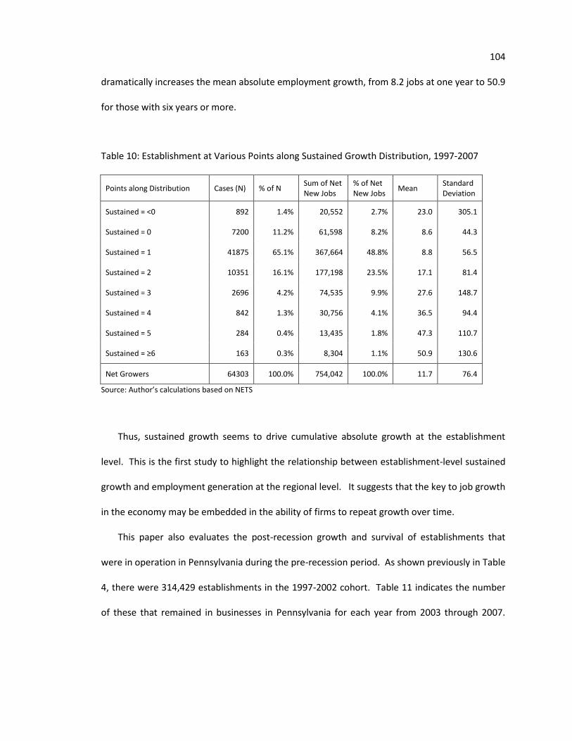
104 dramatically increases the mean absolute employment growth, from 8.2 jobs at one year to 50.9
for those with six years or more.
Table 10: Establishment at Various Points along Sustained Growth Distribution, 1997-2007
Points along Distribution Cases (N) % of N Sum of Net New Jobs
% of Net New Jobs
Mean Standard Deviation
Sustained = <0 892 1.4% 20,552 2.7% 23.0 305.1
Sustained = 0 7200 11.2% 61,598 8.2% 8.6 44.3
Sustained = 1 41875 65.1% 367,664 48.8% 8.8 56.5
Sustained = 2 10351 16.1% 177,198 23.5% 17.1 81.4
Sustained = 3 2696 4.2% 74,535 9.9% 27.6 148.7
Sustained = 4 842 1.3% 30,756 4.1% 36.5 94.4
Sustained = 5 284 0.4% 13,435 1.8% 47.3 110.7
Sustained = ≥6 163 0.3% 8,304 1.1% 50.9 130.6
Net Growers 64303 100.0% 754,042 100.0% 11.7 76.4
Source: Author’s calculations based on NETS
Thus, sustained growth seems to drive cumulative absolute growth at the establishment
level. This is the first study to highlight the relationship between establishment-level sustained
growth and employment generation at the regional level. It suggests that the key to job growth
in the economy may be embedded in the ability of firms to repeat growth over time.
This paper also evaluates the post-recession growth and survival of establishments that
were in operation in Pennsylvania during the pre-recession period. As shown previously in Table
4, there were 314,429 establishments in the 1997-2002 cohort. Table 11 indicates the number
of these that remained in businesses in Pennsylvania for each year from 2003 through 2007.

105 The survival rate falls by approximately 5% per year over the post-recession period, from a high
of 95% in 2003, to 77% in 200722.
Table 11: Descriptive Statistics for Establishment Survival in Pennsylvania from 1997-2002 to 2002-2007
Establishments Number of Survivors
Percentage Standard Deviation
Survived to '03 298576 .95 .22
Survived to '04 283141 .90 .29
Survived to '05 268155 .85 .35
Survived to '06 253592 .81 .39
Survived to '07 242135 .77 .42
Source: Author’s calculations based on NETS
3.6 Independent Variables
Resource-Based View of the firm (RBV) argues that companies that have relatively superior
levels of resources and abilities will out-perform other companies. There are 13 independent
variables that measure different aspects of company operations related to resources and
abilities23. All of these variables are dichotomous.
Businesses that are publicly traded are likely to have better access to capital needed for
R&D and capacity expansion than would private firms. The independent variable ‘Public’ is
compared against the variable ‘Private’, which is not included in the regressions24.
22
Survival is measured for the entire cohort of establishments that were in operation in Pennsylvania during the entire 1997-2002 period. An establishment is considered to have survived to a given year if they remained in business and located in Pennsylvania during that year. 23
I interpret the meaning of each variable according to my personal understanding of the corresponding literature. 24
In order to maintain the necessary degrees of freedom to fit a regression analysis to the data when using dichotomous variables that represent each possible state of a categorical variable, one dichotomous variable must be left out of the regression. The results for the included dichotomous variables are then compared to the omitted version. For example, companies can be either Public or Private. The odds ratio

106 Establishments that are connected through ownership structures to larger organizations are
likely to have a quantitative and/or qualitative resource advantage over stand-alone firms. The
variables that represent connection to larger organizations are ‘Foreign-Owned’, ‘Ownership
Change’, ‘Headquarters’, and ‘Branch’. ‘Foreign-Owned’ is compared with ‘Domestic’, which is
not included in the regressions. Likewise, ‘Headquarters’ and ‘Branch’ are measured against
‘Stand-alone’. ‘Ownership Change’ reports whether the firm has changed headquarters during
the study period. A change in headquarters reflects an acquisition or merger and is assumed to
generally represent a stand-alone firm being acquired by a larger company.
Companies that are better organized are, presumably, better able to coordinate and deploy
resources and abilities, leading to superior performance over other firms. The variables
‘Corporation’ and ‘Partnership’ are compared against ‘Proprietor’. Corporations and
Partnerships are more complex than sole-proprietorships due to their legal structure, tax code
compliance, and use of a board of directors, as well as the internal organization needed to
support higher complexity such as reporting procedures, HR practices, risk control, and strategic
planning among others. Organizations that are relatively less complex are likely to face
challenges as they develop more complex structures to accommodate growth.
Access to a relatively wider geographical range of markets should benefit the firm, by giving
it more opportunities to expand sales and to source unique and competitive supplies. ‘Exporter’
is compared against ‘Non-Exporter’ while ‘Importer’ is compared against ‘Non-Importer’.
Operational flexibility is an indication of managerial ability, as implied by RBV. One measure
of operational flexibility is ‘Primary SIC Changed’, which indicates that the firm has changed the
3-digit SIC code they report as their primary operating activity to Dunn and Bradstreet at some
for Public, when Private is left out of the regression, tells us how much greater the odds of the outcome event are for Public versus Private companies.

107 time during the study period. Companies that have developed value-added services to support
their manufacturing, mining, or agricultural activities also demonstrate operational flexibility.
The variable ‘Services are Non-Primary SIC’ represents establishments that report a 8-digit
services industry SIC as their secondary or tertiary activity but do not report a service industry
SIC as their primary activity.
Finally, companies that have relocated their operations during the study period may have
access to greater levels of resources than firms that have not relocated. Companies that
experience rapid growth consume excess facility space: one of the primary constraints to growth
is the lack of space for warehousing, production, and personnel. On the other hand, relocating
consumes resources in terms of both managerial time and expenses. It is unclear whether
relocation will ultimately increase or decrease establishment-level growth and survival over the
length of the study period. To better discern the effect of relocation, two variables are included
in the 1997-2007 period, indicating whether the firm relocated in the first five years or the
second. These are ‘Relocated ≤ 2001’ and ‘Relocated ≥ 2002’ respectively.
To control for the large proportion of young small establishments, the dichotomous variable
‘Small Size’ represents establishments that have 20 or fewer employees at the beginning of the
study period while ‘First Year’ represents the age of the firm. It follows that a larger number for
the later variable indicates a younger establishment. However, when considering the mean, the
earliest ‘First Year’ recorded is 1989 (the first year this data was compiled in the NETS dataset)
which skews this variable rightward, as will be shown below. In deference to Gibrat, young and
small enterprises are more likely to have higher relative growth but less absolute growth when
compared with larger older firms.

108 Table 12: Descriptive Statistics for Firm Characteristics, 1997-2007
Variables N Minimum Maximum Mean Std. Deviation
Small Size (≤ 20 emps), 1997 240880 .0 1 .912 .283
FirstYear 240880 1989.0 1995 1990.150 1.956
Public 240880 .0 1 .044 .204
Private 240880 .0 1 .956 .204
Foreign-Owned 240880 .0 1 .001 .036
Ownership Changed 240880 .0 1 .069 .254
Corporation 240880 .0 1 .348 .476
Partnership 240880 .0 1 .059 .236
Proprietorship 240880 .0 1 .404 .491
Headquarters 240880 .0 1 .055 .229
Branch 240880 .0 1 .104 .305
Standalone 240880 .0 1 .841 .366
Exporter 240880 .0 1 .018 .134
Importer 240880 .0 1 .008 .091
Primary SIC Changed 240880 .0 1 .108 .310
Services are Non-Primary SIC 240880 .0 1 .045 .207
Relocated ≤ 2001 240880 .0 1 .086 .281
Relocated ≥ 2002 240880 .0 1 .049 .215
Valid N (listwise) 240880
Source: Author’s calculations based on NETS
Table 12 indicates that the vast majority of establishments were small, young, privately-
owned standalone proprietorships; they did not change ownership, SICs, or location, and did not
export or import. Some 9-in-10 establishments had 20 employees or less in 1997. The average
age in 1997, the first year of the study period, was 7 years old. Less than 5% of establishments
were public. Foreign-ownership was very rare at 0.1%. Only 7% of establishments changed

109 ownership over the study period. One third of establishments were corporations while another
6% were partnerships. Some 84% of establishments were standalone. Less than 2% export,
while far fewer import. About 1-in-10 changed their primary SIC, and 1-in-20 reported services
as a secondary or tertiary activity but not their primary business.
The growth of the services industries in recent decades throughout most industrial
economies has been well document. However, there have been surprisingly few studies that
investigate whether services companies are more likely to experience growth, exceptional
growth, or survival when compared with businesses in other industries. This study includes the
sectors of ‘Construction’, ‘Manufacturing’, ‘Agriculture’, and ‘Mining’. The ‘Services’ industry is
the comparison variable and is excluded from the regressions25. Because of the growth of the
services sector in the overall economy, it is anticipated that businesses in the services industry
will have higher odds of growth and survival than will those in other industries.
As discussed earlier, the Pennsylvania Department of Community and Economic
Development (DCED) contracted with IBM to identify and study the 10 ‘industry clusters’ that it
believed held the highest chance for growth in Pennsylvania for the foreseeable future. The
operating assumption of that project was that industry cluster theory had shown that public
organizations could choose ex-ante which industries in their state possess a competitive
advantage over rival locations. They could then organize their economic development efforts,
along with local development partners at the county and city level, to focus upon these clusters;
investing in specialized infrastructure, funding new and highly tailored education and training
25
The Service industry includes businesses in the retail, wholesale, financial, insurance, real estate, transportation, professional services, personal services, and utilities industry segments.

110 programs, and providing direct assistance to these businesses in the form of technical expertise,
technology transfer, low interest loans and grants.26
The exact process for choosing these specific ten industries has not been made public,
however extensive work was involved in preparing reports that detail the trends in these
industries and how they relate to different regions of the state. In addition, DCED used the
study to rally local economic development agencies around coordinated state-wide efforts to
offer support to businesses in these clusters.
The ten industry clusters include bio-pharmaceuticals R&D and production, medical
equipment and devices, “new generation” electronics, alternative energy technology, powdered
metals, prefabricated housing and buildings, agro-food processing, creative and entertainment,
headquarters, and financial services. To create the variables used in this analysis, companies
were considered to be included in the cluster if their 6-digit SIC matched the activities
associated with each industry.
Porter’s cluster theory and other advocates of cluster policies strongly believe that
government is capable of choosing appropriate clusters and to increase the growth in these
industries through tailored policies and programs. Consistent with this belief, it is expected that
firms in all ten of these industry clusters will out-perform other non-cluster companies in terms
of their odds for net growth, exceptional growth, and survival. However, this analysis will not be
able to discern whether cluster policies have directly or indirectly influenced these firms’
performance. The built-in bias towards growth was inherent in the selection process that
DBED and IBM used to select these industries, because their selection was based on at least
26
For more information on Pennsylvania’s Targeted Industry Clusters and associated policies and initiatives, see www.paworkstats.state.pa.us/gsipub/index.asp?docid=407#, www. oewd.psu.edu/files/PA_Cluster2001-04.pdf, and www.teampa.com/newsletter/fullNewsletter_1_08.html.

111 some macro-economic data that illustrated growth trends in Pennsylvania and at the national
level in each of these ten clusters.
Table 13: Descriptive Statistics for Industry Characteristics, 1997-2007
Variables N Minimum Maximum Mean Std. Deviation
Construction Industry 240880 .0 1 .110 .313
Manufacturing Industry 240880 .0 1 .069 .253
Agriculture Industry 240880 .0 1 .032 .175
Mining Industry 240880 .0 1 .002 .042
Services Industry 240880 .0 1 .788 .409
Bio-Pharmaceuticals Cluster 240880 .0 1 .004 .064
Medical Equipment Cluster 240880 .0 1 .004 .062
Electronics Cluster 240880 .0 1 .001 .032
Alternative Energy Cluster 240880 .0 1 .000 .010
Powdered Metals Cluster 240880 .0 1 .008 .087
Prefab Buildings Cluster 240880 .0 1 .044 .206
AgroFood Processing Cluster 240880 .0 1 .020 .139
Creative & Entertainment Cluster
240880 .0 1 .005 .072
Headquarter Cluster 240880 .0 1 .003 .056
Financial Services Cluster 240880 .0 1 .046 .209
Valid N (listwise) 240880
Source: Author’s calculations based on NETS
Table 13 shows that most establishments were in the services industry, with few
participating in any of the Clusters. Consistent with popular perception, the services industry
dominates the Pennsylvania economy in terms of total number of businesses. Nearly 79% of all
establishments reported that their primary business was services. In total, only 13.5% of all

112 Pennsylvania establishments were included in the state’s top ten strategic industry clusters.
More than half of all cluster businesses were found in just two clusters: financial services and
prefabricated buildings.
The central implication of urbanization theory is that human density contributes to
economic growth. Population density creates thick markets for labor, products and services,
and capital. It also facilitates the sharing of ideas which fosters innovation. By extension, a
rapidly growing local population should accelerate these effects. The result should be that firms
that are located in more densely populated areas will have a greater chance to grow and survive
than firms located in more sparsely populated areas. The variable ‘Population Density’ is a
measure of the number of people in each county divided by the size of the county in square
miles. In addition, ‘% Population Change’ measures the percentage of increase in population in
the county where each firm is located during the five year period immediately preceding the
study period.
The United States Department of Agriculture created the Rural-Urban Continuum Codes
(RUCC) to classify counties by their degree of urbanism. There are three metropolitan county
codes, depending on the size of the urban population in that county, and six non-metropolitan
codes that distinguish counties by the size of their urban population and whether they are
adjacent to a metropolitan county. These codes are shown in Table 14 below.

113 Table 14: County Rural-Urban Continuum Codes and Descriptions
Code Description
Metro counties:
RUCC 9 Counties in metro areas of 1 million population or more
RUCC 8 Counties in metro areas of 250,000 to 1 million population
RUCC 7 Counties in metro areas of fewer than 250,000 population
Nonmetro counties:
RUCC 6 Urban population of 20,000 or more, adjacent to a metro area
RUCC 5 Urban population of 20,000 or more, not adjacent to a metro area
RUCC 4 Urban population of 2,500 to 19,999, adjacent to a metro area
RUCC 3 Urban population of 2,500 to 19,999, not adjacent to a metro area
RUCC 2 Completely rural or less than 2,500 urban population, adjacent to a metro area
RUCC 1 Completely rural or less than 2,500 urban population, not adjacent to a metro area
Source: USDA; see www.ers.usda.gov/Data/RuralUrbanContinuumCodes
The county code ‘RUCC9’ is used as the comparison variable and is thus excluded from the
regression. In accordance with the implication of urbanization theory, the odds of growth and
survival should be higher for establishments located in the largest urban area (‘RUCC9’) than in
other counties, and higher in counties that are adjacent to a metro area when compared with
those not adjacent to a metro area.
Localization theory strongly implies that innovation and productivity gains are more easily
achieved by firms located in relatively close proximity to competitors, suppliers, and customers.
If this theory is correct, the performance improvements provided by localization should
manifest themselves in superior establishment level growth.
The United States Department of Agriculture has created the 2004 County Typology Codes
which are relied upon in this analysis. These codes reflect the presence of the dominant

114 economic specialization (or lack of specialization) for each county in the United States. Each
county is assigned only one typology code, which are described in the Table 15 below. The
regressions include ‘Service County Economy’, ‘Manufacturing County Economy’, ‘Mining
County Economy’, and ‘Federal or State County Economy’. For unknown reasons, none of the
67 counties in Pennsylvania were classified by USDA as ‘Farming-dependent’. Based on
localization theory, firms located in specialized counties should out-perform firms located in
‘Nonspecialized’, which is the comparison variable.
Table 15: County Economic Specialization Codes and Descriptions
Variable Name Definition
Service County Economy 45% or more of average annual labor and proprietor’s earnings derived from services during 1998-2000
Manufacturing County Economy 25% or more of average annual labor and proprietor’s earnings derived from manufacturing during 1998-2000
Mining County Economy 15% or more of average annual labor and proprietor’s earnings derived from mining during 1998-2000
Federal or State County Economy 15% or more of average annual labor and proprietor’s earnings derived from Federal or State government during 1998-2000
Non-Specialized Did not meet the dependency threshold for any one of the above industries
Source: USDA; www.ers.usda.gov/Briefing/Rurality/Typology/
The variables ‘# Firms in same Sector & County, 1997’ was created based on the 2-digit SIC
code that is recorded as the establishment’s primary industry of operation. These were grouped
together into five sectors: Services, Manufacturing, Construction, Mining, and Agriculture.
Table 16 indicates that half of all Pennsylvania establishments were located in counties that
were in metropolitan areas that have 1 million population or more. On average, establishments’
county of residence experienced population growth of 2.6% between 1991 and 1996. The
average percentage of local population with a college degree was 23%. Nearly half of the firms
were located in counties that specialized in the services economy, while another third were in

115 counties specializing in manufacturing. There were no establishments located in RUCC5 or in
counties specializing in farming. On average, each establishment was located in a county with
more than 14,000 other firms in their same sector.
Table 16: Descriptive Statistics of Location Characteristics, 1997-2007
Variables N Minimum Maximum Mean Std. Deviation
Population Density, 1996 240880 11.401 11412.333 1614.601 2966.5046
% Population Change, 1991-1996 240880 -.025 .291 .026 .0414
Rural, ≤ 2.5k urban pop, non-metro (RUCC1)
240880 .000 1.000 .002 .0485
Rural, ≤ 2.5k urban pop, metro (RUCC2)
240880 .000 1.000 .002 .0429
Urban pop 2.5-19.9k, non-metro (RUCC3)
240880 .000 1.000 .015 .1218
Urban pop 2.5-19.9k, metro (RUCC4)
240880 .000 1.000 .041 .1983
Urban pop ≥ 20k, non-metro (RUCC5)
240880 .000 .000 .000 .0000
Urban pop ≥ 20k, metro (RUCC6) 240880 .000 1.000 .103 .3034
In metro area of < 250k pop (RUCC7)
240880 .000 1.000 .053 .2247
In metro area of 250k-1m pop (RUCC8)
240880 .000 1.000 .281 .4495
Counties in metro area of ≥ 1 million pop (RUCC9)
240880 .000 1.000 .503 .5000
% College Educated, 2000 240043 8.800 42.500 23.085 8.6080
Service County Economy 240880 .000 1.000 .467 .4989
Manufacturing County Economy 240880 .000 1.000 .333 .4712
Mining County Economy 240880 .000 1.000 .009 .0970
Federal or State County Economy 240880 .000 1.000 .038 .1909
Farming County Economy 240880 .000 .000 .000 .0000
Non-specialized County Economy 240880 .000 1.000 .153 .3602
# Firms in same Sector & County, 1997
240561 1.000 45744.000 14363.115 14898.1709
Valid N (listwise) 239725
Source: Author’s calculations based on NETS

116 Section 4.5 provides descriptions and analysis of the establishment growth variables. Gibrat
expects reversion to the mean for net, absolute, and relative growth. On average, a period of
positive growth should be followed by a period with negative growth. Because Gibrat does not
directly address the concept of sustained growth over numerous years, the relationship
between the first five-year period and the second will follow RBV, and be predicted to be
positive.
Table 17 summarizes the source, expected signs, and appropriate theoretical relationships
for each independent variable as discussed above.

117 Table 17: Expected Signs of the Independent Variables based on Theoretical Guidance
Dependent Variables
Independent Variables Source Growth Survival Theoretical Guidance
Firm Characteristics
Small Size (≤ 20 emps, '97) NETS + - Gibrat’s Law
Headquarters NETS + + Resource-Based View
Branch NETS + + Resource-Based View
First Year NETS - + Gibrat’s Law
Foreign-Owned NETS + + Resource-Based View
Exporter NETS + + Resource-Based View
Importer NETS + + Resource-Based View
Public NETS + + Resource-Based View
Corporation NETS + + Resource-Based View
Partnership NETS + + Resource-Based View
Relocated ≤ 2001 NETS + + Resource-Based View
Relocated ≥ 2002 NETS + + Resource-Based View
Changed Primary SIC NETS + + Resource-Based View
Changed Duns# (Ownership) NETS + + Resource-Based View
Secondary or Tertiary Services (not Primary) NETS + + Resource-Based View
Industry Characteristics
Construction industry NETS - -
Manufacturing industry NETS - -
Agriculture industry NETS - -
Mining industry NETS - -
BioPharmaceuticals Cluster DCED + + Cluster Theory
Medical Equipment Cluster DCED + + Cluster Theory
Electronics Cluster DCED + + Cluster Theory
Alternative Energy Cluster DCED + + Cluster Theory
Powdered Metals Cluster DCED + + Cluster Theory
Prefab Buildings Cluster DCED + + Cluster Theory
AgroFood Processing Cluster DCED + + Cluster Theory
Creative & Entertainment Cluster DCED + + Cluster Theory
Headquarters Cluster DCED + + Cluster Theory
Financial Services Cluster DCED + + Cluster Theory
Location Characteristics
Rural, ≤ 2.5k urban pop, non-metro USDA - - Urbanization
Rural, ≤ 2.5k urban pop, metro USDA - - Urbanization
Urban pop 2.5-19.9k, non-metro USDA - - Urbanization
Urban pop 2.5-19.9k, metro USDA - - Urbanization
Urban pop ≥ 20k, metro USDA - - Urbanization
In metro area of < 250k pop USDA - - Urbanization
In metro area of 250k-1m pop USDA - - Urbanization
Population Density, '96 USCB + + Urbanization
% Population Change, '91-'96 USCB + + Resource-Based View
% College Educated, 2000 USCB + + Resource-Based View
Manufacturing economy USDA - - Localization
Mining economy USDA - - Localization
Federal or State economy USDA - - Localization
Non-Specified economy USDA - - Localization
Firms in same industry & county NETS + + Localization
Firm Growth (1997-2002)
Net Growth NETS 0 0 Gibrat’s Law
Absolute Growth, Top 10% NETS - - Gibrat’s Law
Relative Growth, Top 10% NETS - - Gibrat’s Law
Sustained Growth at 2 yrs NETS + + Resource-Based View
Note: NETS = National Employment Time-Series; DCED = Pennsylvania Department of Community and Economic Development; USDA = United States Department of Agriculture; USCB = United States Census Bureau.

CHAPTER 4: ANALYSIS
This chapter begins with a test for Power Law in the distribution of establishment growth
then proceeds with logistics regressions as described previously. It concludes with a summary of
the findings.
4.1 Test for Power Law
The finding of a Laplace rather than a Gaussian distribution for establishment-level absolute
employment growth leads to the question of whether this growth distribution follows a Power
Law. Newman (2005) discusses two different approaches: visual inspection for linearity in a log-
log distribution plot, and calculating the exponent of the scale-invariant relationship.
To begin, Figure 6 presents the distribution of absolute growth for the 1997-2007 period
with the true values of absolute growth plotted against the log of their frequency. This simple
conversion into a log-normal distribution makes it easier to observe that even with logged
frequencies the distribution retains high kurtosis and a fat tail to the right, indicative of Laplace.

119 Figure 6: Log-Normal Distribution of Absolute Growth, 1997-2007
Figure 7 presents the log-log distribution of absolute growth for the 64,303 establishments
with positive net employment growth during the 1997-2007 period27. For visual inspections,
linearity needs to be present across only part of the distribution to conclude that a Power Law is
applicable (Stanley and Plerou 2001; Durlauf 2005; Newman 2005). Some deterioration of the
goodness-of-fit is common in log-log distributions when the total number of cases is not
extremely large. Despite some variance between bins, a cursory look at Figure 7 shows that
linearity is present across most of the distribution, with the possible exception of the extreme
right end of the distribution.
27
See Table 7 for more details.

120 Figure 7: Log-Log Distribution of Absolute Growth, 1997-2007
A Power Law is a scale-invariant distribution such that if f(g) ~ g-α where f(g) represents the
number of firms that have growth of g or greater than g, the exponent α represents the
probability density. Newman (2005) reports that most Power Laws that occur in nature have an
exponent in the range of 2 ≤ α ≤ 3. He offers the following equation to calculate the exponent
α:
α = 1 + 𝑛 ln𝑥𝑖𝑥𝑚𝑖𝑛
𝑛
𝑖=0
−1
and to calculate the statistical error, σ:
σ = 𝑛 ln𝑥𝑖𝑥𝑚𝑖𝑛
𝑛
𝑖=0
−1
= α − 1
𝑛

121 The set of establishments displayed in Figure 7 contains 43,528 cases (n) with log values
above 0.0. These have a minimum value of 0.69 and a maximum of 9.10. When applied to the
formulas above, the result is 2.23 +/- 0.002. This falls within the range of 2 ≤ α ≤ 3, leading to
the conclusion that a Power Law governs the distribution of absolute growth for the cohort of
Pennsylvania establishments over the 1997-2007 period.
As reviewed earlier, linearity implies universality in accordance with Power Law theory,
where heterogeneous but interdependent agents create scale invariant distributions due to
increasing returns operating at some level within a complex system. These relationships,
whether involving purposeful cooperation (as implied by cluster theory) or resulting from battles
between contestants of heterogeneous abilities (as implied by RBV), manifest themselves into
linearity in log-log displays when some agents accumulate a disproportionate amount of
resources28.
The underlying causal relationships that determine linearity cannot be discerned from
Figure 729. However, Stanley and Plerou (2001) suggest that log-log distributions can be
compared between groups of different cases to see if there are visual differences that indicate
whether a Power Law may be in effect for one group and not for another. Accordingly,
Appendix B compares log-log distributions for a variety of dichotomous variables that are
important to both cluster and agglomeration theories (largest metro vs. other counties; services
vs. manufacturing sector; cluster vs. non-cluster establishments). Visual comparison of these
plots fails to find notable differences between these groups of establishments. This suggests
that these variables (urbanization, sector, cluster designation) do not fundamentally determine
28
The underlying dynamics of heterogeneous independent agents may also produce Power Law behavior in closely related phenomenon that empower or result from Power Law behavior in firm growth distributions (e.g. firm profits or regional growth, respectively). Further investigation in this direction may yield insight into the universality of growth. 29
They are further explored in the logistics regressions in the following section.

122 whether a group of establishments exhibit the increasing return behavior indicative of Power
Law distributions.
4.2 Regression Results
Table 18 provides a cross-reference for each research question; indicating which of the
tables below contains the corresponding study period, independent variables, and model tested.
Table 18: Research question results by table and test description
Question Table Period Dependent Variable Models
Q1a Table 19 1997-2007 Net Employment Growth Firm, Industry, Location, All
Q1b Table 20 3 periods Net Employment Growth All
Q2a Table 21 1997-2007 Absolute Employment Growth ≤ 1%, ≤ 10%, No Growth, ≥90%, ≥ 99%
Q2b Table 22 1997-2007 ≥90% Growth Absolute, Relative, Sustained Growth
Q 3a Table 23 1997-2007 Net Employment Growth (’02-07) Net, Absolute, Relative, Sustained Growth
Q 3b Table 24 1997-2007 Survival to 2007 Net, Absolute, Relative, Sustained Growth
4.2.1 Question 1: Explaining Past Growth
Q1a: What is the relative strengths of firm, industry, cluster policy, or locational characteristics to explain employment growth over a ten year period (1997-2007)?
Table 19 shows the results from logistic regression using the dependent variable net
establishment-level growth over the 1997-2007 period. The first three models include
independent variables related to firm, industry, and location characteristics respectively. The
fourth model combines all of the variables30.
30
Note that the headquarters variable is used as both a firm and an industry characteristic, and has consequently been included only once in Model 4. Also note that the number of cases in Models 3 and 4 declines from 240,880 to 239,725 due to incomplete location data for approximately 1000 cases.

123 Table 19: Logistics Regression of Establishment-level Net Employment Growth in Pennsylvania for Firm, Industry, Location, and All Variables, 1997-2007 (odds ratios)
Independent Variables Firm Industry/Cluster Location All
Exp(B) SE Exp(B) SE Exp(B) SE Exp(B) SE
Firm Characteristics
Small Size (≤ 20 emps), 1997 1.250*** .017
1.263*** .017
First Year 1.019*** .002
1.021*** .002
Public .809*** .026
.796*** .027
Foreign-Owned 1.277** .115
1.254** .115
Ownership Changed 1.038 .024
1.031 .024
Corporation 2.098*** .011
2.128*** .011
Partnership 1.710*** .020
1.713*** .020
Headquarters1 1.216*** .020
1.213*** .020
Branch 2.050*** .022
2.041*** .022
Exporter 1.351*** .033
1.288*** .034
Importer 1.208*** .048
1.231*** .048
Primary SIC Changed 1.258*** .014
1.252*** .015
Services are Non-Primary SIC 1.127*** .022
1.150*** .025
Relocated ≤ 2001 1.559*** .016
1.596*** .016
Relocated ≥ 2002 1.367*** .021
1.396*** .021
Industry and Cluster Characteristics
Construction Industry .952*** .016 .954** .019
Manufacturing Industry 1.368*** .019 1.068*** .023
Agriculture Industry .712*** .035 .860*** .037
Mining Industry 1.451*** .101 1.047 .104
BioPharmaceuticals Cluster 1.322*** .068 1.113 .070
Medical Equipment Cluster 1.317*** .071 1.177** .072
Electronics Cluster 1.419*** .130 1.177 .133
Alternative Energy Cluster .891 .426 .616 .432
Powdered Metals Cluster .964 .053 .978 .055
Prefab Buildings Cluster .906*** .025 .868*** .025
AgroFood Processing Cluster 1.020 .043 1.018 .044
Creative & Entertainment Cluster 1.471*** .059 1.140** .061
Headquarters Cluster1 1.701*** .074
Financial Services Cluster 1.210*** .021 1.083*** .022
Location Characteristics
Population Density, 1996
.999** .000 .999*** .000
% Population Change, 1991-1996
1.238 .142 1.345** .150
Rural, ≤ 2.5k urban pop, non-metro (RUCC1)
1.025 .098 1.099 .100
Rural, ≤ 2.5k urban pop, metro (RUCC2)
.680*** .122 .785* .124
Urban pop 2.5-19.9k, non-metro (RUCC3)
1.030 .042 1.068 .043
Urban pop 2.5-19.9k, metro (RUCC4)
1.035 .030 1.126*** .031
Urban pop ≥ 20k, metro (RUCC6)
1.029 .023 1.064*** .023
In metro area of < 250k pop (RUCC7)
1.077*** .025 1.098*** .026
In metro area of 250k-1m pop (RUCC8)
1.012 .015 .999 .017
% College Educated, 2000
1.006*** .001 1.000 .001
Service County Economy
.950** .022 .936*** .023
Manufacturing County Economy
1.035** .015 1.052*** .015
Mining County Economy
1.021 .050 1.054 .051
Federal or State County Economy
.972 .030 1.007 .031
# Firms in same Sector & County, 1997
.999 .000 1.000 .000
Constant .000*** 4.885 .356*** .005 .315*** .027 .000*** 4.919
Total Observations in analysis 240880 240880 239725 239725
Negelkerke R Square .051 .005
.001 .054
Cox & Snell R Square .035 .003
.001 .037
Model Chi-square 8505.864*** 804.382***
188.087*** 9044.286***
Degrees of Freedom 15 14
15 43
Classification - Overall Percent Correct 73.3 73.3
73.3 73.4
Hosmer and Lemeshow .000 .000 .003 .007
*** significant at 0.01 level 1Same Variable
** significant at 0.05 level
* significant at 0.1 level

124 Of the first three models in Table 19, the one with firm characteristics has the strongest
explanatory power. The Negelkerke R Square for the firm variables model is .051, which is 10-
times higher than the industry/cluster variable model, and more than 50-times higher than the
location variable model. Similar relationships are found using the alternative Cox & Snell R
Square. The Omnibus Chi-Square test confirms that the model adequately fits the data. Overall,
these results strongly suggest that firm characteristics dominate industry, cluster policy, and
location characteristics in explaining establishment-level net employment growth for
Pennsylvania businesses during the 1997-2007 period.
Almost every firm characteristic is significant in both the first model and the fourth which
combines all variables. Consistent with Gibrat, smaller and younger firms are more likely to
grow. The signs and significance of all but one of the other 13 firm variables are consistent with
the predictions of Resource-Based View (RBV).
Companies that were better organized (corporations, partnerships) performed better than
sole proprietorships; establishments with ownership links to larger organizations (foreign-
owned, headquarters, branches, acquisitions) had a higher tendency to grow than stand-alone
firms; and companies with larger geographic selling and sourcing territories (exporters,
importers) tended to out-perform others. Operational flexibility and adaptation (value-added
services, changing SIC codes, and relocating) also tended to increase the propensity to grow.
However, contrary to expectation, public companies were significantly less likely to grow than
private firms.
The second model, which includes industry characteristics, indicates that 11 of the 14
industry variables are significant, however only seven are significant when included with the
other variables in the fourth model. When compared with the services industry, establishments

125 in manufacturing and mining were more likely than those in the services sector to grow,
whereas those in construction and agriculture were less likely to expand employment.
The cluster variables show mixed results. Only three clusters (Medical Equipment, Creative
& Entertainment, and Financial Services) increase odds of net growth and are significant in both
the industry model and when included with the other variables31. Three clusters reduce the
odds of net growth in both models, but only Prefab Buildings is significant. Consequently, the
results for five clusters – half of the cluster set - are inconclusive. These inconsistencies cast
substantial doubt about the power of the cluster approach to explain establishment-level
growth in Pennsylvania during this ten year period, especially when considering the upward bias
built into the choice of these clusters by IBM and DCED.
Only 5 of the 15 location variables are significant in both the third and the fourth model.
The most comprehensive variable that measures urbanization is county-level population
density, which significantly reduces odds of net growth. This indicates that companies in
counties with higher population densities were less likely to grow than firms in less densely
populated counties, contradicting a strong prediction of urbanization theory. Interestingly,
businesses located in counties with relatively high proportion of population growth were more
likely to grow. The Rural Urban County Continuum (RUCC) variables show mixed results. When
compared with the largest urban areas (RUCC9, the comparison variable), companies in smaller
urban areas (RUCC 4, 6, 7) have a higher chance to grow. Non-metro county variables increase
growth odds but are insignificant. Education concentration in the local county has an
indeterminable impact on firm-level growth.
31
Headquarters also significantly increases odds of net growth. This cluster variable also describes a corporate function and is thus included with Firm characteristics in Model 4.

126 The variable that most closely measures localization is the number of firms in the same 2-
digit SIC in the same county. While this variable alternates signs between the third and fourth
model it remains insignificant. When the specialization of the county economy is compared
with non-specified counties, manufacturing economies tend to support establishment growth,
while service economies deter it. Economic specialization does not show a significant effect for
either mining or government activities. Overall, the regression results cast doubt upon the
abilities of both urbanization and localization agglomeration theory to explain establishment-
level employment growth in Pennsylvania over the ten-year study period.
Q1b: What is the relative strength of firm, industry, cluster policy, or locational characteristics
to explain firm employment growth over five-year pre-recession and post-recession periods (1997-2002 and 2002-2007)?
Table 20 reports results for logistic regressions on the dependent variable of net growth for
three periods: the five years preceding and following the economic recession of 2001 (1997-
2002 and 2002-2007), and the entire 10-year period (1997-2007). The 1997-2007 results are the
same as the fourth model in Table 19, and are included in Table 20 for comparison purposes.
Despite differences in the years studied, macro-economic conditions, and the length of the
study periods, the results shown in Table 20 are remarkably similar across the different periods.
While the Negelkerke R Square and Cox & Snell R Square are both higher in the pre-recession
period of 1997-2002 than in the post-recession period of 2002-2007, the difference is not
dramatic.

127 Table 20: Logistic Regression of Establishment-level Net Employment Growth in Pennsylvania over Different Periods: 1997-2002, 2002-2007, 1997-2007 (odds ratios)
Independent Variables 1997-2002 2002-2007 1997-2007
Exp(B) SE Exp(B) SE Exp(B) SE
Firm Characteristics
Small Size (≤ 20 emps), 1997 1.231*** .017 1.251*** .018 1.263*** .017
First Year .999 .002 1.017*** .001 1.021*** .002
Public .868*** .025 .783*** .025 .796*** .027
Foreign-Owned 1.258** .107 1.287** .105 1.254** .115
Ownership Changed 1.073*** .022 1.055** .022 1.031 .024
Corporation 2.014*** .011 2.161*** .012 2.128*** .011
Partnership 1.597*** .020 1.800*** .021 1.713*** .020
Headquarters1 1.440*** .019 .935*** .024 1.213*** .020
Branch 1.883*** .021 2.165*** .019 2.041*** .022
Exporter 1.485*** .033 1.209*** .038 1.288*** .034
Importer 1.335*** .046 1.351*** .050 1.231*** .048
Primary SIC Changed 1.267*** .014 1.496*** .014 1.252*** .015
Services are Non-Primary SIC 1.258*** .024 1.087*** .028 1.150*** .025
Relocated ≤ 2001 1.669*** .015 1.596*** .016
Relocated ≥ 2002 1.577*** .018 1.396*** .021
Industry and Cluster Characteristics
Construction Industry .963* .019 .912*** .021 .954** .019
Manufacturing Industry 1.084*** .022 1.108*** .023 1.068*** .023
Agriculture Industry .589*** .041 1.058 .039 .860*** .037
Mining Industry .935 .101 .911 .118 1.047 .104
BioPharmaceuticals Cluster 1.007 .067 1.330*** .063 1.113 .070
Medical Equipment Cluster 1.245*** .068 1.110 .072 1.177** .072
Electronics Cluster 1.068 .126 1.308** .129 1.177 .133
Alternative Energy Cluster .773 .390 1.125 .340 .616 .432
Powdered Metals Cluster 1.205*** .052 1.056 .057 .978 .055
Prefab Buildings Cluster .842*** .025 .982 .027 .868*** .025
AgroFood Processing Cluster 1.026 .046 .961 .046 1.018 .044
Creative & Entertainment Cluster 1.287*** .053 .964 .054 1.140** .061
Headquarters Cluster1
Financial Services Cluster 1.047** .022 1.099*** .022 1.083*** .022
Location Characteristics
Population Density, 1996 .999*** .000 0.999*** .000 .999*** .000
% Population Change, 1991-1996 0.725* .148 1.574*** .167 1.345** .150
Rural, ≤ 2.5k urban pop, non-metro (RUCC1) 1.146 .097 .986 .109 1.099 .100
Rural, ≤ 2.5k urban pop, metro (RUCC2) .802* .122 .985 .126 .785* .124
Urban pop 2.5-19.9k, non-metro (RUCC3) 1.062 .042 1.149*** .044 1.068 .043
Urban pop 2.5-19.9k, metro (RUCC4) 1.032 .031 1.166*** .033 1.126*** .031
Urban pop ≥ 20k, metro (RUCC6) 1.008 .023 1.092*** .024 1.064*** .023
In metro area of < 250k pop (RUCC7) 1.050* .025 1.170*** .026 1.098*** .026
In metro area of 250k-1m pop (RUCC8) .983 .016 1.071*** .017 .999 .017
% College Educated, 2000 1.000 .001 1.001 .001 1.000 .001
Service County Economy 0.919*** .022 .919*** .023 .936*** .023
Manufacturing County Economy 1.057*** .015 1.051*** .016 1.052*** .015
Mining County Economy 1.038 .051 1.098* .053 1.054 .051
Federal or State County Economy .967 .030 1.030 .031 1.007 .031
# Firms in same Sector & County, 1997 1.000 .000 1.000 .000 1.000 .000
Constant 1.432 4.788 .000*** 2.247 .000*** 4.919
Total Observations in analysis 311300 355010 239725
Negelkerke R Square .052 .041 .054
Cox & Snell R Square .032 .023 .037
Model Chi-square 10250.738*** 8322.401*** 9044.286***
Degrees of Freedom 42 42 43
Classification - Overall Percent Correct 80.9 85.2 73.4
Hosmer and Lemeshow .000 .000 .007
*** significant at 0.01 level 1Same Variable
** significant at 0.05 level
* significant at 0.1 level

128 The influence on the odds of net growth and the significance of the firm-level variables in
the two five-year periods are generally similar to the patterns seen in the 10-year period. In
both 1997-2002 and 2002-2007, smaller size increases the odds for growth, although younger
age is only significant in the later period. The results from all other firm-level variables are
consistent with the predictions of RBV. The exception is that in both periods, public firms have
less chance of growth than privately-held companies. However, more formal organization,
being part of a larger organization, more extensive selling and sourcing networks, and
operational flexibility are all associated with a higher propensity to grow.
An interesting difference in firm-level variables between the two periods is that while
branches tend to out-perform stand-alone businesses in both periods, headquarters out-
perform standalones only in the pre-recession years, while they tend to under-perform
standalones during the post-recession period. It is possible that this is due to some tendency for
HQs to trim staff and overhead costs in response to economic downturns as demand falls to
levels below the pre-recession peak.
The results for industry variables are similar across all three periods as well. Establishments
in the manufacturing and mining industries have a higher probability of growth than do those in
the services industry, whereas construction and agriculture businesses have reduced odds of
growth.
The results of the cluster variables are again mixed. Four of the 10 clusters (when including
headquarters) switch between increasing and decreasing net growth odds between the two
five-year periods. Six of the 10 clusters are significant in one five-year period but not in the
other. Perhaps most importantly, only one cluster (financial services) significantly increases

129 odds of net growth in both the pre-recession and post-recession period32. While large variation
in results for the cluster variables may reflect changes in the macro–economy, they could also
reflect different phases of the business cycle within each industry. Nevertheless, these findings
raise doubts about the ability of government agencies to identify ex-ante which industry clusters
will generate employment growth.
In both the pre- and post-recession periods county population density significantly
decreases odds for net growth. Companies in many secondary metro areas tended to out-
perform those in the most highly populated urban areas, particularly in the second period.
Perhaps more puzzling is that the influence of population growth changes dramatically between
the two periods. During 1997-2002, companies in counties with high population growth were
much less likely to grow, while companies in those same counties were much more likely to
grow during 2002-2007. This may reflect a lag between the upward shift in local demand
generated by rapid population growth and the time it takes for firms to respond by increasing
locally produced supply. However, further investigation is needed to better understand this
phenomenon.
Among specialized county economies, only those focused on manufacturing significantly
out-performed non-specialized economies in both periods. Companies in counties specializing
in the services industry tended to under-perform those in non-specialized counties. It is also
important to note that the number of firms in the same industry and county was insignificant in
both periods.
Overall, these results show remarkable similarity in both periods. Taken together, they offer
strong support for RBV while failing to support the implied predictions of cluster, urbanization,
32
It would be tempting to conclude that financial services are therefore less volatile than other clusters, however major losses and bankruptcies in that industry during 2008-2009 appear to argue otherwise.

130 and localization theories. They tell us that despite the conditions in the macro economy in
Pennsylvania over these two periods, firm-level characteristics dominate industry, cluster, and
location as an explanation for establishment-level growth.
4.2.2 Question 2: Alternative Definitions of Growth
Q2a: How do the explanatory strengths of these independent variables differ at different points along the growth distribution (re: from negative to high growth)?
Table 21 reports the results from logistics regression on absolute employment growth at
different points along the growth distribution. These include the bottom 1% and 10% of the
growth distribution (re: negative growth), no growth (the median and mode), and the top 10%
and 1% of the growth distribution. The period of study is 1997-2007. Each regression contains
the same firm, industry/cluster, and location variables used in the previous tables.
The Omnibus chi-square test reports that all models adequately fit the data, however that is
only confirmed for the first model when using the Hosmer and Lemshow test. Based on the R-
square scores, the models have slightly higher explanatory power towards the higher end of the
growth spectrum.
Looking at firm characteristics, and excluding the results of the bottom 1%, the results show
substantial changes along the growth distribution for almost every variable. Smaller size
increases the odds of stagnation (no growth) and greatly reduces the odds of extreme growth in
the top 10% and 1%. On the other hand, relatively young establishments have greater odds of
extreme growth.

131 Table 21: Logistic Regression of Establishment-level Absolute Growth at the 1 percentile, 10 percentile, no growth, 90 percentile, and 99 percentile, 1997-2007 (odds ratios)
Independent Variables ≤ 1% ≤ 10% No Growth ≥ 90% ≥ 99%
Exp(B) SE Exp(B) SE Exp(B) SE Exp(B) SE Exp(B) SE
Firm Characteristics
Small Size (≤ 20 emps), 1997 .000 85.390 .397*** .018 1.187*** .016 0.559*** .019 .150*** .048
First Year 1.007 .013 .952*** .004 .998 .002 1.044*** .004 1.070*** .012
Public 1.215*** .061 1.056*** .031 1.168*** .025 .850*** .033 1.421*** .069
Foreign-Owned .979 .218 .936 .135 .757** .134 1.346** .122 1.898*** .183
Ownership Changed 1.331*** .055 1.146*** .027 .880*** .023 1.144*** .028 1.377*** .061
Corporation .598*** .096 1.628*** .015 .515*** .010 4.527*** .018 15.292*** .140
Partnership .794* .137 1.328*** .028 .650*** .018 2.929*** .031 11.023*** .165
Headquarters1 1.717*** .056 1.163*** .025 .821*** .020 1.533*** .023 2.234*** .055
Branch .859 .104 1.878*** .027 .515*** .020 4.106*** .029 14.309*** .150
Exporter 1.189** .075 1.193*** .039 .620*** .038 1.293*** .038 1.241*** .079
Importer 1.405*** .089 .993 .056 .784*** .052 1.360*** .053 1.274** .100
Primary SIC Changed 1.183*** .056 1.090*** .019 .784*** .014 1.302*** .019 1.316*** .054
Services are Non-Primary SIC .915 .098 1.149*** .032 .819*** .023 1.172*** .033 1.119 .094
Relocated ≤ 2001 .895* .065 .988 .022 .681*** .015 1.899*** .020 2.039*** .053
Relocated ≥ 2002 1.582*** .085 1.173*** .028 .714*** .020 1.666*** .027 1.642*** .081
Industry and Cluster Characteristics
Construction Industry 1.208 .121 .879*** .027 1.148*** .017 1.185*** .028 1.206* .103
Manufacturing Industry 1.641*** .074 1.308*** .028 .808*** .021 1.179*** .029 1.478*** .079
Agriculture Industry 2.329*** .283 .721*** .056 1.248*** .032 .567*** .072 .875 .272
Mining Industry 1.285 .309 1.144 .126 .961 .102 1.203 .125 2.078*** .276
BioPharmaceuticals Cluster .894 .207 1.078 .087 .873** .067 1.221** .084 1.597*** .171
Medical Equipment Cluster .881 .163 1.045 .081 .824** .077 1.295*** .082 1.296 .171
Electronics Cluster .966 .281 .811 .159 1.011 .140 1.149 .149 1.916** .258
Alternative Energy Cluster 1.459 .549 1.210 .417 1.357 .436 0.402* .512 .000 7369.931
Powdered Metals Cluster .793 .165 1.354*** .061 .819*** .054 .971 .068 .935 .175
Prefab Buildings Cluster .736** .149 1.109*** .033 1.064*** .022 .821*** .036 .846 .128
AgroFood Processing Cluster .803 .151 .870*** .060 1.090** .039 1.344*** .065 1.791*** .138
Creative & Entertainment Cluster 1.327 .233 .833** .089 .965 .059 1.295*** .075 1.796*** .178
Headquarters Cluster1
Financial Services Cluster 1.339*** .093 1.004 .029 .889*** .021 .779*** .033 .924 .092
Location Characteristics
Population Density, 1996 1.000 .000 1.000 .000 1.000*** .000 .999*** .000 1.000 .000
% Population Change, 1991-1996 .318 .768 .395*** .207 1.339** .134 1.594** .218 17.914*** .713
Rural, ≤ 2.5k urban pop, non-metro (RUCC1) .907 .627 1.109 .137 .835** .088 1.244 .153 .527 .734
Rural, ≤ 2.5k urban pop, metro (RUCC2) .660 .754 1.082 .157 1.213** .101 .859 .208 1.287 .615
Urban pop 2.5-19.9k, non-metro (RUCC3) 1.248 .187 1.134** .056 .952 .038 1.124** .064 .810 .239
Urban pop 2.5-19.9k, metro (RUCC4) .827 .169 .976 .043 .918*** .028 1.123** .048 1.034 .168
Urban pop ≥ 20k, metro (RUCC6) .940 .115 1.025 .031 .945*** .021 1.076** .035 0.802** .121
In metro area of < 250k pop (RUCC7) .838 .124 1.032 .035 .923*** .023 1.132*** .037 1.191 .118
In metro area of 250k-1m pop (RUCC8) 1.010 .080 1.068*** .022 .985 .015 1.049** .025 .980 .081
% College Educated, 2000 .994 .006 .999 .002 1.002 .001 1.002 .002 .988** .006
Service County Economy 1.050 .109 .973 .030 1.047** .020 0.911*** .033 .976 .106
Manufacturing County Economy .902 .074 .990 .021 .942*** .014 1.046** .023 .950 .075
Mining County Economy .978 .264 1.158** .067 .856*** .046 1.068 .078 1.188 .282
Federal or State County Economy 1.008 .141 .940 .042 .996 .027 1.033 .044 1.288 .136
# Firms in same Sector & County, 1997 1.000 .000 1.000 7.449E-07 1.000 .000 1.000*** .000 1.000*** .000
Constant .000 26.330 1.673E+41 6.975 41.019 4.379 .000 7.093 .000*** 23.613
Total Observations in analysis 239725 239725
239725 239725
239725
Negelkerke R Square .483 .065
.065 .145
.244
Cox & Snell R Square .054 .035
.049 .073
.026
Model Chi-square 13406.303*** 8513.601***
11979.697*** 18226.326***
6288.621***
Degrees of Freedom 43 43
43 43
43
Classification - Overall Percent Correct 98.9 87.2
59.6 88.8
99.0
Hosmer and Lemeshow 1.000 .000 .000 .001 .000
*** significant at 0.01 level 1Same Variable
** significant at 0.05 level
* significant at 0.1 level

132 There is a remarkable and unexpected pattern among most of the other firm variables. The
odds of extreme growth increase (and the odds of stagnation decrease) for firms with a formal
organization, those part of a larger organization, those having a wide sourcing and selling
territory, and those with greater operational flexibility, as expected by RBV. Yet, these same
characteristics also increase the odds that the establishment will be in the bottom 10% of
growth. This suggests that there are substantial risks associated with the development and
deployment of resources and skills at the establishment level.
It is costly for the firm to incorporate, develop and deploy new value-added services, expand
into new markets, and relocate their operations. It seems that a significant number of
companies mismanaged these investments or are overcome by market forces which make the
costs too great to bear, resulting in downsized operations33. This finding cautions that the
gathering and development of resources and skills as described by RBV does not have a
uniformly positive outcome on the growth of the firm. Further research is needed to discern at
a finer level the internal differences between firms that succeed and those that do not.
The industry variables show a mixed pattern. While the manufacturing industry
demonstrates a pattern similar to the RBV variables described above (re: less likely to stagnate,
more likely to have extreme performance), firms in construction and mining tend to have
greater odds of growth. For some clusters (such as biopharmaceuticals, medical devices,
creative industries) the propensity for growth is higher than for stagnation. Yet, for two clusters
(alternative energy, prefab buildings) establishments have higher odds than others of stagnation
rather than extreme growth. The chances of extreme job loss in the financial services industry
appear greater than the chances for either stagnation or extreme growth. These mixed results
33
If studied with aggregated data, this somewhat off-setting trend may appear to be a reversion-to-the-mean effect, and may partly account for Gibrat’s view that firm growth is stochastic.

133 offer limited support for cluster theory in regards to three of the 10 clusters but undermines the
theory’s general applicability due to the large variation across the different clusters.
If cluster theory performed as expected by its policy advocates there would be a clear
pattern in the influence of cluster membership on establishment growth, particularly at the
extreme ends of the absolute growth distribution. For example, we would expect to see that
establishments in clusters had significantly higher odds of being in the top 1% or 10% of the
distribution and significantly lower odds of being in the bottom 1% and 10% of the distribution.
However, this expected pattern is not evident in Table 21.
Relatively high levels of population density increase the odds of establishment-level
stagnation but decrease the odds for growth in the top 10% of the distribution, challenging the
basic tenets of urbanization theory. However, higher levels of county population growth
dramatically improve the probability for exceptional growth. The odds of extreme growth are
higher in most of the secondary metro areas than for the comparison variable (counties with
urban population ≥ 1 million). Taken together, these results suggest that changes at the margin
of local population size are more important for firm-level growth than the absolute size and
density of the local population.
The economic specialization of counties tends to increase the odds of establishment-level
growth in manufacturing, mining, and government services, but it reduces the odds in service
specialized counties. However, a high number of companies in the same sector and county does
tend to increase the odds of exceptional growth, providing modest support for localization
theory.
Q2b: How do the explanatory strengths of these independent variables differ by the way employment growth is measured (re: absolute, relative, or sustained)?

134 Table 22 displays results from logistic regressions of the top 90% of Absolute, Relative, and
Sustained growth for the 1997-2007 period. The results for Absolute are taken from the fifth
model in Table 21 and are presented for comparison.
The Omnibus tests indicate that all models adequately fit the data. Both R Square
measures show that the explanatory power of the model is highest for Absolute growth.
Overall, the results are similar across the three measures of growth however a few variables do
switch signs across the three models.
As expected, small size is positively associated with extreme relative growth but negatively
related to extreme absolute growth. As noted in the literature review, the measure of absolute
growth is biased towards larger firms while relative growth is biased towards smaller firms.
Smaller establishments are more likely to sustain growth over multiple years than are larger
establishments. The other firm characteristic variables behave in a similar fashion across the
different growth measures.
There is variation across the dependent variables in regards to industry. Establishments in
the construction industry are more likely to have extreme absolute and relative growth but less
likely to sustain growth. On the other hand, agriculture businesses are less likely to have
extreme absolute and sustained growth but more likely to have high relative growth. This raises
questions as to whether industry is a dependable measure of employment growth at the
establishment-level.
Overall, there are more cluster variables that are significant for extreme absolute growth
than for relative or sustained growth. Six significantly increase odds for absolute, while only
two have similar effect for relative growth and four for sustained growth. Only two significantly
increase odds across all measures of growth (headquarters and creative and entertainment),
while one significantly decreases odds across the measures (prefabricated buildings). In other

135 words, only three-of-ten clusters have a consistent impact on high growth, independent of how
growth is measured, and the effect one of these clusters is opposite from the theory’s
predictions.

136 Table 22: Logistic Regression of Establishment-level Absolute, Relative, and Sustained Growth at 90 percentile, 1997-2007 (odds ratios)
Independent Variables Absolute Relative Sustained
Exp(B) SE Exp(B) SE Exp(B) SE
Firm Characteristics
Small Size (≤ 20 emps), 1997 0.559*** .019 3.223*** .031 1.214*** .018
First Year 1.044*** .004 1.072*** .003 1.019*** .003
Public .850*** .033 .751*** .041 .808*** .028
Foreign-Owned 1.346** .122 1.559*** .141 1.193 .117
Ownership Changed 1.144*** .028 1.171*** .034 .999 .024
Corporation 4.527*** .018 1.431*** .014 2.105*** .012
Partnership 2.929*** .031 1.300*** .025 1.717*** .021
Headquarters1 1.533*** .023 1.212*** .026 1.137*** .021
Branch 4.106*** .029 1.031 .031 1.973*** .023
Exporter 1.293*** .038 1.081 .047 1.237*** .035
Importer 1.360*** .053 1.340*** .065 1.258*** .049
Primary SIC Changed 1.302*** .019 1.316*** .018 1.248*** .015
Services are Non-Primary SIC 1.172*** .033 1.061* .030 1.128*** .025
Relocated ≤ 2001 1.899*** .020 1.671*** .019 1.576*** .016
Relocated ≥ 2002 1.666*** .027 1.606*** .024 1.358*** .021
Industry and Cluster Characteristics
Construction Industry 1.185*** .028 1.126*** .024 .960** .020
Manufacturing Industry 1.179*** .029 1.059** .029 1.034 .023
Agriculture Industry .567*** .072 1.260*** .043 .868*** .039
Mining Industry 1.203 .125 1.535*** .125 1.014 .108
BioPharmaceuticals Cluster 1.221** .084 1.074 .090 1.100 .071
Medical Equipment Cluster 1.295*** .082 1.087 .100 1.187** .073
Electronics Cluster 1.149 .149 1.144 .178 1.146 .136
Alternative Energy Cluster 0.402* .512 .517 .753 .516 .471
Powdered Metals Cluster .971 .068 .889 .075 1.082 .055
Prefab Buildings Cluster .821*** .036 .833*** .032 .857*** .026
AgroFood Processing Cluster 1.344*** .065 1.056 .052 1.052 .045
Creative & Entertainment Cluster 1.295*** .075 1.315*** .071 1.189*** .062
Headquarters Cluster1
Financial Services Cluster .779*** .033 .921*** .031 1.080*** .023
Location Characteristics
Population Density, 1996 .999*** .000 .999*** .000 .999*** .000
% Population Change, 1991-1996 1.594** .218 2.203*** .185 1.304* .155
Rural, ≤ 2.5k urban pop, non-metro (RUCC1) 1.244 .153 1.066 .124 1.106 .103
Rural, ≤ 2.5k urban pop, metro (RUCC2) .859 .208 .904 .147 .805* .128
Urban pop 2.5-19.9k, non-metro (RUCC3) 1.124** .064 1.038 .055 1.044 .044
Urban pop 2.5-19.9k, metro (RUCC4) 1.123** .048 1.089** .039 1.129*** .032
Urban pop ≥ 20k, metro (RUCC6) 1.076** .035 1.030 .029 1.051** .024
In metro area of < 250k pop (RUCC7) 1.132*** .037 1.027 .033 1.086*** .026
In metro area of 250k-1m pop (RUCC8) 1.049** .025 .976 .021 .990 .017
% College Educated, 2000 1.002 .002 .998 .002 1.001 .001
Service County Economy 0.911*** .033 .973 .029 .921*** .023
Manufacturing County Economy 1.046** .023 1.019 .019 1.060*** .016
Mining County Economy 1.068 .078 .919 .067 1.027 .053
Federal or State County Economy 1.033 .044 .994 .039 .996 .032
# Firms in same Sector & County, 1997 1.000*** .000 1.000 .000 1.000 .000
Constant .000 7.093 .000*** 5.919 .000*** 5.084
Total Observations in analysis 239725 239725
239725
Negelkerke R Square .145 .036
.049
Cox & Snell R Square .073 .020
.032
Model Chi-square 18226.326*** 4767.495***
7908.919***
Degrees of Freedom 43 43
43
Classification - Overall Percent Correct 88.8 86.1
76.0
Hosmer and Lemeshow .001 .000 .008
*** significant at 0.01 level 1Same Variable
** significant at 0.05 level
* significant at 0.1 level

137 High population density decreases the odds of growth at the firm-level for all three growth
measures. In addition, secondary urban areas generally increase odds of growth when
compared with the largest urban areas. Surprisingly perhaps, the percentage of college
educated workers is not significant for any growth measure. The number of firms in the same
sector and county is only significant for absolute growth. Taken together, these results suggest
that county-level specialization has only a weak effect, at best, on exceptional growth at the
firm-level.
4.2.3 Question 3: Predicting Future Growth and Survival
Q3a: How well do firm, industry, cluster, location, and past growth predict future growth (re: growth in 1997-2002 vs. growth in 2002-2007)?
Table 23 reports results for logistic regressions on establishment-level net growth. The
dataset includes all companies that were in operation in Pennsylvania from 1997 through 2007.
It uses the establishments’ 1997-2002 demographics and performance to predict their growth
during the 2002-2007 period. Thus, the dependent variable is net employment growth during
2002-2007. All independent variables related to firm, industry/cluster, and location
characteristics are included. There are four new independents introduced to the model,
representing establishment performance in the 1997-2002 period. These indicate whether the
establishment experienced net growth and, if so, whether they were also in the top 10% of
absolute, relative, or sustained growth during 1997-200234.
The Omnibus test indicates that the models adequately fit the data, which is also confirmed
for four of the five models with the Hosmer and Lemeshow test. Table 23 also shows that the
model’s predictive ability improves when prior net, absolute, and sustained growth are added.
34
Sustained growth is a dichotomous variable indicating whether the firm added net new employees during at least two of the five years in the 1997-2002 period.

138 Taken together, this suggests that past growth does predict future growth, at least to some
extent. It thus rejects the view that firm-level growth is entirely stochastic from one period to
the next.
The results for almost all dependent variables related to firm, industry, and location
characteristics are nearly the same across the five versions of the model. Only one variable
(manufacturing industry) varies in being significant over the different versions.
All firm-growth variables significantly increase the odds that a firm operating in
Pennsylvania in 1997-2002 would grow in the subsequent 2002-2007 period. Past sustained
growth increases the odds of future growth more than the other measures of growth. In fact,
when included in the model, past sustained growth increases the odds of future growth by more
than 40 of the 42 other independent variables. Furthermore, sustained growth has a stronger
positive influence on future growth than any industry/cluster or location variable.

139 Table 23: Logistic Regression to Predict Establishment-level Net Growth during 2002-2007 based on 1997-2002 Performance (odds ratios)
Independent Variables F, I/C, L F, I/C, L & Net F, I/C, L & Absolute F, I/C, L & Relative F, I/C, L & Sustained
Exp(B) SE Exp(B) SE Exp(B) SE Exp(B) SE Exp(B) SE
Firm Characteristics
Small Size (≤ 20 emps), 1997 1.101*** .021 1.093*** .021 1.109*** .021 1.092*** .021 1.108*** .021
First Year 1.002 .003 1.002 .003 1.001 .003 1.002 .003 1.001 .003
Public .743*** .033 .747*** .033 .746*** .033 .744*** .033 .743*** .033
Foreign-Owned 1.236* .127 1.221 .127 1.219 .127 1.229 .127 1.210 .128
Ownership Changed 1.043 .028 1.039 .028 1.036 .028 1.042 .028 1.035 .028
Corporation 2.095*** .014 2.040*** .014 2.032*** .014 2.088*** .014 2.054*** .014
Partnership 1.696*** .024 1.669*** .025 1.670*** .025 1.692*** .024 1.680*** .025
Headquarters1 .921*** .025 .906*** .025 .901*** .026 .918*** .025 .911*** .026
Branch 1.767*** .026 1.729*** .026 1.724*** .026 1.766 .026 1.760*** .026
Exporter 1.278*** .040 1.253*** .040 1.250*** .040 1.276*** .040 1.249*** .040
Importer 1.364*** .055 1.345*** .055 1.340*** .055 1.359*** .055 1.334*** .055
Primary SIC Changed 1.386*** .017 1.372*** .017 1.374*** .017 1.382*** .017 1.374*** .017
Services are Non-Primary SIC 1.144*** .029 1.134*** .029 1.135*** .029 1.143*** .029 1.139*** .029
Relocated ≤ 2001 1.160*** .019 1.132*** .019 1.131*** .019 1.152*** .019 1.131*** .019
Industry and Cluster Characteristics
Construction Industry .945** .024 .945** .024 .941** .024 .944** .024 .944** .024
Manufacturing Industry 1.065** .027 1.059 .027 1.056 .027 1.064** .027 1.058 .027
Agriculture Industry 1.052 .043 1.067 .043 1.063 .043 1.053 .043 1.059 .043
Mining Industry .928 .127 .929 .127 .924 .127 .925 .127 .934 .127
BioPharmaceuticals Cluster 1.175** .079 1.172** .079 1.171** .079 1.175** .079 1.169** .079
Medical Equipment Cluster 1.029 .085 1.018 .085 1.016 .085 1.028 .085 1.023 .085
Electronics Cluster 1.165 .148 1.161 .148 1.159 .148 1.161 .148 1.136 .148
Alternative Energy Cluster .430 .609 .436 .610 .442 .609 .430 .609 .436 .610
Powdered Metals Cluster 1.103 .064 1.093 .064 1.095 .064 1.103 .064 1.094 .064
Prefab Buildings Cluster .963 .030 .969 .030 .969 .030 .965 .030 .967 .030
AgroFood Processing Cluster .985 .051 .985 .051 .983 .051 .984 .051 .985 .051
Creative & Entertainment Cluster .766*** .078 .756*** .078 .751*** .078 .763*** .078 .741*** .078
Headquarters Cluster1
Financial Services Cluster 1.175*** .027 1.174*** .027 1.179*** .027 1.177*** .027 1.176 .027
Location Characteristics
Population Density, 1996 .999** .000 .999** .000 .999** .000 .999** .000 .999** .000
% Population Change, 1991-1996 1.636*** .180 1.653*** .180 1.650*** .180 1.637*** .180 1.647*** .180
Rural, ≤ 2.5k urban pop, non-metro (RUCC1) 1.032 .125 1.026 .125 1.027 .125 1.030 .125 1.025 .125
Rural, ≤ 2.5k urban pop, metro (RUCC2) .925 .146 .930 .146 .925 .146 .924 .146 .932 .146
Urban pop 2.5-19.9k, non-metro (RUCC3) 1.128** .052 1.126** .052 1.126** .052 1.127** .052 1.127** .052
Urban pop 2.5-19.9k, metro (RUCC4) 1.185*** .037 1.184*** .037 1.184*** .037 1.185*** .037 1.185*** .037
Urban pop ≥ 20k, metro (RUCC6) 1.114*** .028 1.114*** .028 1.113*** .028 1.113*** .028 1.115*** .028
In metro area of < 250k pop (RUCC7) 1.179*** .031 1.177*** .031 1.177*** .031 1.179*** .031 1.180*** .031
In metro area of 250k-1m pop (RUCC8) 1.050** .020 1.051** .020 1.050** .020 1.051** .020 1.052** .020
% College Educated, 2000 1.002 .001 1.002 .001 1.002 .001 1.002 .001 1.002 .001
Service County Economy .927*** .028 .930*** .028 .930*** .028 .927*** .028 .930*** .028
Manufacturing County Economy 1.095*** .019 1.093*** .019 1.094*** .019 1.095*** .019 1.093*** .019
Mining County Economy 1.079 .062 1.077 .062 1.078 .062 1.079 .062 1.078 .062
Federal or State County Economy 1.050 .037 1.050 .037 1.049 .037 1.050 .037 1.049 .037
# Firms in same Sector & County, 1997 1.000 .000 1.000 .000 1.000 .000 1.000 .000 1.000 .000
Firm Growth (1997-2002)
Net Growth 1.265*** .014
Absolute Growth, Top 10%
1.296*** .016
Relative Growth, Top 10%
1.103*** .018
Sustained Growth at 2 yrs
1.729*** .026
Constant .001 5.924 .001 5.929 .003 5.930 .002 5.930 .013 5.934
Total Observations in analysis 311300 311300
311300 311300
311300
Negelkerke R Square .031 .032
.032 .031
.033
Cox & Snell R Square .015 .016
.016 .015
.017
Model Chi-square 4833.147*** 5121.184***
5095.804*** 4861.794***
5234.476***
Omnibus df 42 43
43 43
43
Classification - Overall Percent Correct 88.8 88.8
88.8 88.8
88.8
Hosmer and Lemeshow .217 .136 .031 .308 .072
*** significant at 0.01 level
** significant at 0.05 level
* significant at 0.1 level
1Same Variable

140 Q3b: How well do firm, industry, cluster, location, and past growth predict future survival?
(re: growth in 1997-2002 vs. survival through 2007)? Table 24 reports the results of logistic regression on establishment-level survival. It includes
all establishments that operated in Pennsylvania from 1997 to 2002; many of which went out of
business during the 2002-2007 period35. The model uses each establishment’s demographic
and performance characteristics from 1997-2002 to predict survival to the year 2007. Thus, the
dependent variable is establishment survival in Pennsylvania through 2007. Along with firm,
industry/cluster, and location variables, it also includes performance variables such as net,
absolute, relative, and sustained growth from 1997-2002, similar to Table 23.
Table 24 shows that the inclusion of a growth variable from the 1997-2002 period improves
the ability of the model to predict survival to 2007. The Omnibus Chi-Square test shows that all
models adequately fit the data. Therefore, a firm’s past growth partially predicts its future
survival.
According to the R Square measures, the model which includes net growth in the 1997-2002
has the strongest predictive power. However, when looking at the individual growth variables,
sustained growth increases the odds of survival more than any of the other growth variables.
The significance of all but one of the independent variables are the same in each version of
the model. Only the specialized service economy variable changes from being significant in
three versions and insignificant in the other two, although the influence on the odds of survival
are essentially the same.
These results provide further support for the view that business growth is not completely
stochastic, but that past growth significantly increases the odds of future establishment-level
survival.
35
See Table 11 for the distribution of establishment survival.

141 Table 24: Logistic Regression to Predict Establishment-level Survival until 2007 based on 1997-2002 Performance (odds ratios)
Independent Variables F, I/C, L F, I/C, L & Net F, I/C, L & Absolute F, I/C, L & Relative F, I/C, L & Sustained
Exp(B) SE Exp(B) SE Exp(B) SE Exp(B) SE Exp(B) SE
Firm Characteristics
Small Size (≤ 20 emps), 1997 .987 .018 .972 .018 .992 .018 .970* .018 .988 .018
First Year .924*** .002 .924*** .002 .924*** .002 .924*** .002 .924*** .002
Public 1.031 .025 1.041 .025 1.038 .025 1.034 .025 1.032 .025
Foreign-Owned .959 .131 .941 .132 .940 .132 .947 .131 .946 .131
Ownership Changed .939*** .022 .936*** .022 .933*** .022 .938*** .022 .936*** .022
Corporation 1.528*** .011 1.472*** .011 1.471*** .011 1.517*** .011 1.510*** .011
Partnership 1.413*** .020 1.382*** .020 1.387*** .020 1.407*** .020 1.405*** .020
Headquarters1 1.293*** .024 1.261*** .024 1.256*** .024 1.283*** .024 1.285*** .024
Branch 1.021 .020 .985 .020 .986 .020 1.017 .020 1.017 .020
Exporter 1.438*** .044 1.392*** .044 1.393*** .044 1.432*** .044 1.418*** .044
Importer 1.185*** .059 1.164*** .059 1.160** .059 1.176*** .059 1.171*** .059
Primary SIC Changed 1.341*** .016 1.323*** .016 1.328*** .016 1.333*** .016 1.335*** .016
Services are Non-Primary SIC 1.278*** .025 1.264*** .025 1.268*** .025 1.275*** .025 1.275*** .025
Relocated ≤ 2001 .803*** .015 .776*** .015 .779*** .015 .792*** .015 .793*** .015
Industry and Cluster Characteristics
Construction Industry .946*** .017 .948*** .018 .943*** .017 .944*** .017 .946*** .017
Manufacturing Industry .818*** .021 .814*** .021 .811*** .021 .818*** .021 .815*** .021
Agriculture Industry .835 .031 .852*** .031 .846*** .031 .839*** .031 .838*** .031
Mining Industry .773** .104 .774** .104 .768** .104 .769** .104 .776** .104
BioPharmaceuticals Cluster .823 .065 .823*** .065 .820*** .065 .823*** .065 .821*** .065
Medical Equipment Cluster 1.019 .080 1.001 .081 1.000 .081 1.015 .080 1.015 .080
Electronics Cluster .917 .141 .911 .142 .909 .142 .910 .142 .902 .142
Alternative Energy Cluster .720 .435 .734 .436 .741 .436 .719 .435 .718 .435
Powdered Metals Cluster 1.372*** .061 1.356*** .061 1.362*** .061 1.371*** .061 1.367*** .061
Prefab Buildings Cluster .936*** .023 .943*** .023 .941*** .023 .939** .023 .937*** .023
AgroFood Processing Cluster .884*** .037 .884*** .037 .883*** .037 .883*** .037 .884*** .037
Creative & Entertainment Cluster .563*** .050 .553*** .050 .551*** .050 .558*** .050 .554*** .050
Headquarters Cluster1
Financial Services Cluster 1.049** .022 1.046** .022 1.053** .022 1.051** .022 1.049** .022
Location Characteristics
Population Density, 1996 1.000 .000 1.000* .000 1.000 .000 1.000 .000 1.000 .000
% Population Change, 1991-1996 .614*** .135 .625*** .135 .622*** .135 .615*** .135 .616*** .135
Rural, ≤ 2.5k urban pop, non-metro (RUCC1) .937 .089 .929 .089 .934 .089 .935 .089 .935 .089
Rural, ≤ 2.5k urban pop, metro (RUCC2) .846** .095 .854* .095 .848* .095 .847* .095 .849* .095
Urban pop 2.5-19.9k, non-metro (RUCC3) .974 .040 .971 .040 .972 .040 .973 .040 .974 .040
Urban pop 2.5-19.9k, metro (RUCC4) .910*** .028 .908*** .028 .910*** .028 .910*** .028 .910*** .028
Urban pop ≥ 20k, metro (RUCC6) .986 .021 .985 .021 .985 .021 .985 .021 .986 .021
In metro area of < 250k pop (RUCC7) 1.081*** .024 1.078*** .024 1.079*** .024 1.080*** .024 1.080*** .024
In metro area of 250k-1m pop (RUCC8) .997 .015 .997 .015 .996 .015 .997 .015 .997 .015
% College Educated, 2000 1.000 .001 1.000 .001 1.000 .001 1.000 .001 1.000 .001
Service County Economy .955** .020 .959** .021 .958** .021 .956** .021 .956** .021
Manufacturing County Economy 1.057 .014 1.054*** .014 1.056 .014 1.057*** .014 1.056*** .014
Mining County Economy 1.086** .048 1.084* .048 1.087* .048 1.087* .048 1.086* .048
Federal or State County Economy .971 .028 .973 .028 .971 .028 .972 .028 .970 .028
# Firms in same Sector & County, 1997 .999*** 5.220E-07 .999*** 5.23E-07 .999*** 5.230E-07 .999*** 5.230E-07 .999*** 5.230E-07
Firm Growth (1997-2002)
Net Growth 1.452*** .012
Absolute Growth, Top 10%
1.459*** .015
Relative Growth, Top 10%
1.255*** .015
Sustained Growth at 2 yrs
1.488*** .029
Constant 1.05E+68*** 4.138 9.58E+67 4.145 4.66E+68*** 4.143 6.07E+68*** 4.142 3.09E+68*** 4.140
Total Observations in analysis 311300 311300 311300 311300 311300
Negelkerke R Square .027 .032
.031 .029
.028
Cox & Snell R Square .018 .021
.020 .019
.019
Model Chi-square 5681.587*** 6685.734***
6378.867*** 5915.174***
5890.614***
Omnibus df 42 43
43 43
43
Classification - Overall Percent Correct 77.0 77.0
77.0 77.0
77.0
Hosmer and Lemeshow .002 .000 .001 .000 .000
*** significant at 0.01 level 1Same Variable
** significant at 0.05 level
* significant at 0.1 level

CHAPTER 5: CONCLUSIONS
The objective of this dissertation has been to test competing theories that attempt to
explain business growth and survival. These include industry cluster theory and its antecedents
in agglomeration and industrial organization theories, the Resource-Based View, and Gibrat’s
Law of Proportionate Effect. The analysis used a time-series dataset containing more than
300,000 business establishment that operated in Pennsylvania during the 1997-2007 period. It
evaluated 44 independent variables representing firm characteristics, industry and cluster
characteristics, and location characteristics for each establishment. It also included four
independent variables related to growth in a prior period. The dependent variables included
establishment’s net employment growth, absolute and relative employment change, the
number of years of net growth, and survival. In addition, it tested the distribution of
establishment growth for evidence of Power Law relationships to help explain the existence of a
sub-set of establishments that demonstrate superior growth and to address the question of
whether business growth is stochastic or systematic.
The explanatory power of the model that only contained firm characteristics to explain
establishment-level growth was 10-times higher than the model with only industry and cluster
characteristics, and it was more than 50-times higher than the model containing only location
characteristics. These relationships were found to be consistent over ten years, for both the
pre-recession and post-recession periods, and for various measures of employment growth.
This indicates that firm characteristics dominate industry, cluster, and location characteristics in
explaining establishment-level growth within the study group.

143 Consistent with Resource-Based View (RBV), companies that were better organized, with
external links to larger organizations, more extensive selling and buying networks, and those
with operational flexibility and adaptation traits were the most likely to expand net employment
and survive. These relationships held for all periods studied, including both pre- and post-
recession years, and for various definitions of growth (absolute, relative, and sustained). Yet,
the contribution of RBV-related variables to establishment performance was not unidirectional.
While they reduced the odds of stagnation, they also increased the probability of both extreme
growth and extreme loss when measured at the top and bottom 10% of the growth distribution.
The results implied that developing and deploying attributes associated with RBV increases both
the risk and reward to the firm. This conclusion must be considered when designing
development policies aimed at increasing RBV-related firm attributes, as discussed below.
The effect of industry and cluster affiliation on establishment growth and survival was mixed
and ultimately inconclusive. Businesses in manufacturing and mining were more likely to grow
than those in services sectors, while those in agriculture and construction were less likely to
grow than those in services sectors. Establishments in state-designated industry clusters were
inconsistent in their employment performance when compared with other businesses.
Membership in four clusters significantly increased the odds of net growth over ten years, while
one cluster significantly decreased the odds of growth, and five clusters were insignificant.
However, these results were likely inflated due to selection bias in the choice of clusters by IBM
and the Pennsylvania Department of Community and Economic Development. More troubling
was that the impact of cluster affiliation changed depending on the period studied and the
definition of growth. Only one cluster, Financial Services, had a positive and significant effect on
the odds for net employment growth for both the pre-recession and post-recession periods.
Some clusters increased the odds of stagnation while others increased the odds of both positive

144 and negative extreme employment change. These findings lead to the conclusion that cluster
policies are unlikely to be an efficient means to increase growth of businesses or regions
because governments cannot accurately choose ex-ante which ‘clusters’ are most likely to grow
in the future.
Locations with the highest level of urban density suppressed establishment-level growth,
contrary to predictions by agglomeration and cluster theories. County population density
significantly decreased the odds of growth for all periods studied, and irrespective of whether
growth was measured in terms of absolute, relative, or sustained employment gains. Higher
density also increased the odds of employment stagnation while decreasing the odds of growth
in the top 10% of the absolute growth distribution. For all regressions, businesses located in
some of the smaller urban and non-urban areas tended to outperform establishments located in
the largest urban areas. In contrast, population growth had a positive and significant influence
on growth odds over ten years and during the five year post-recession period however it had a
negative and significant impact on net growth odds during the pre-recession period. This raises
serious questions about potential negative impacts of urbanization policies on firm and regional
growth.
The effects of localization were conflicting or insignificant. The number of establishments in
the same sector and county did not increase the odds of net growth as expected by localization
theory. In fact, it decreased the odds of business survival. While locating in a manufacturing-
specialized county tended to increase establishments’ chances of growth and survival, locating
in service-specialized counties decreased these outcomes. Surprisingly, the proportion of
college-educated population had no significant impact on establishment-level growth or survival
regardless of the growth measurement or time period studied. These findings again undermine

145 the rationale for cluster and other related development policies that seek to increase economic
specialization of firms and regions.
The growth distribution of establishments located in Pennsylvania during the years of 1997-
2007 was found to resemble a Laplace rather than a Gaussian shape. When plotted on a log-log
distribution, firms with positive net growth exhibited linearity along most of the distribution
while the exponent of the scale-invariant distribution indicated that a Power Law was
applicable. This suggested that a complex system was present within establishment-level
growth which, according to the literature, implies increasing returns among heterogeneous but
interdependent agents, where a subset of agents accumulate a disproportionate share of
growth. Furthermore, there were no visible differences between log-log distributions for
establishments in clusters vs. non-clusters; for establishments in the largest metro areas versus
those not in those areas; and for establishments in services versus manufacturing sectors. This
provides further doubt that industry, cluster, or location are the underlying dynamics that cause
a small sub-set of establishments to accumulate a disproportionate share of growth.
Knowing an establishment’s past growth does improve the ability to predict its future
growth and survival. When included with firm, industry, cluster, and location characteristics,
past growth (measured as in the top 10% of absolute, relative, or sustained growth in the
previous five-year period) improves the power of the model to predict net growth and survival
over the subsequent five years. Past sustained growth had the greatest predictive power;
beating 40 of the other 42 variables included in the models. This provides support for the view
that a substantial number of firms do learn how to repeat and maintain growth over multiple
periods. It highlights the importance of exploring new policies that increase the ability of firms
to sustain growth over multiple years, as discussed below.

146 These findings lead to the acceptance of the first hypothesis, that firm growth follows a
Power Law. However, they rejected the following two hypotheses, that firm, industry, cluster,
and location all have consistently significant power in explaining and predicting establishment-
level growth and survival in past and future periods. While firm characteristics did consistently
help to explain and predict growth and survival, the effects of industry and cluster were mixed
and they varied too substantially by study period, definition of growth, and points along the
growth distribution to adhere to cluster theory. In addition, the effect of location was often
found to be opposite from the predictions of agglomeration theory. Higher levels of
urbanization significantly reduced the odds of growth and survival in most of the regression
results, while localization at the county-level had mixed and weak effects at best.
As stated earlier, the intention of this dissertation was not to build a model with the highest
possible explanatory power, but rather to test the relative strength of variables that are strongly
associated with competing theoretical views of establishment employment growth and survival.
Researchers may wish to strengthen the power of the models presented here by including
additional variables that address other environmental factors, establishment or management
characteristics, or inter-establishment relations. For example, other environmental variables
might include transportation access, local taxation, zoning and site-specific regulations, or the
form of local government. Researchers may also wish to use alternative dependent variables,
such as composite measures of employment growth, sales growth, or changes in productivity.
While there are many possibilities to explore other important questions of interest to
researchers and policy makers and to inform the growth literature, these were beyond the
scope of this study.
This study did provide a number of contributions to the literature on firm and regional
growth. It used RBV as a counterfactual to test the limits of cluster theory and its antecedents in

147 the agglomeration and industrial organization literatures. It demonstrated the importance of
using disaggregated establishment-level datasets in studies of business growth and survival. It
also used several new RBV-related variables to track firm activities (re: ‘Primary SIC Changed’
and ‘Services are Non-Primary SIC’). It was the first study to test Gibrat’s theory by evaluating
future growth and survival of establishments. It was the first to test in one model firm, industry,
cluster, and location variables during pre- and post-recession periods, at different points along
the growth distribution, and using different definitions of establishment-level growth. Perhaps
most importantly, it was the first to explore the relationship between absolute and sustained
growth at the establishment level, and to recognize the impact of sustained growth of
businesses on regional employment changes.
The insights gained from this analysis may prove critical in developing a new theory that
links the growth of firms and regions. There are systematic forces evident of complex systems
that concentrate employment growth within a sub-set of a region’s businesses. Approximately
1% of Pennsylvania’s establishments were responsible for generating 169% of all net new jobs
created in the state over the 1997-2007 period36. Yet, absolute growth by exceptional firms tells
only part of the story. While the average firm that grew only one-of-ten years added 8.6 net
new jobs, firms that grew six or more years added more than 50 jobs37. In fact, the correlation
between absolute and sustained growth is positive and significant for all establishments, and
not just for exceptional firms38. Thus, regional employment growth appears to be driven by the
cumulative impact of sustained growth by establishments over multiple years.
Furthermore, the scale invariant distribution in establishment-level growth demonstrates
the hallmark characteristics of a Power Law. In accordance with Power Law theory, market-
36
See Table 7. 37
See Table 10. 38
See Table 8.

148 place interactions among heterogeneous and independent firms enable a sub-set of businesses
to accumulate a disproportionate share of employment growth. These superior growth shares
are not the result of one-off growth events, but are the cumulative product of multiple years of
growth.
I believe that the results of this research offer an opportunity to propose a new theory to
explain firm growth. It combines insights from the Resource-Based View and Power Law
distributions. Accordingly, the ‘Theory of Cumulative Growth’ posits that business growth is a
cumulative process where a sub-set of firms that are best able to repeat growth over multiple
years will accumulate a disproportionate share of employment growth. Cumulative growth also
increases the odds of business survival. This theory is supported by three findings of this study:
that a sub-set of companies do accumulate a disproportionate share of absolute growth; that
absolute growth rises as growth is accumulated over time; and that sustained growth is one of
the strongest predictors of future growth and survival. In addition, exceptional growth appears
to be related to learning, adaptation, and flexible business operations.
The phenomenon of cumulative establishment-level growth may also explain the primary
driver of regional growth. As discussed in Section 2.3.4, the vast majority of regional
employment growth can be attributed to the growth of existing firms39. Building on that insight,
this study found that the majority of job growth among Pennsylvania’s existing firms was
attributable to a very small group that demonstrated exceptional growth over time. Again, this
large contribution to state-level employment growth by this sub-set of firms is largely
attributable to their ability to sustain growth over multiple years. Thus, Cumulative Growth
Theory may prove a link between the growth of firms and regions.
39
Neumark et al. (2005) found that the growth and decline of existing businesses had the greatest impact on state-level net job changes over multiple years; while the impact of firm births/deaths and in-bound/out-bound relocations were negligible.
149 Future research may discover that the growth distribution of regions exhibits a Power Law
pattern similar to the growth distribution of establishments. If true, this may be due to the
principle of self-similarity which is reflected in some scale-invariant distributions, where the
parts of self-similar objects display the same shape as the whole. For example, regions that
accumulate a disproportionate share of employment growth when compared with other regions
may be the ones that have accumulated growth due to a disproportionate share of high-growth
firms in their regions.
By the extension of the principle of self-similarity, it is also plausible that firms that
accumulate disproportionate shares of growth are the same ones that accumulate
disproportionate shares of profits. As discussed in Section 2.3.3, Power Law behavior has been
found in firm profit distributions. Businesses are only able to sustain growth indefinitely if they
are profitable. Consequently, profitability is a necessary condition for growth accumulation. I
thus hypothesize that there is a high correlation between the firms possessing superior profit
shares and firms with superior employment growth shares.
This line of thinking can be extended deeper to the market-place transactions that drive
profits among firms. According to microeconomics, buyers seek transactions that maximize
their utility from among possible sellers, bounded by constraints of imperfect knowledge.
Sellers that offer utility maximizing transactions are likely to become highly successful and reap
superior profits, bounded by their own constraints of operational costs. If utility maximization
among transactions adheres to universality and the self-similarity principle, the subset of sellers
offering maximum utility over time should accumulate a disproportionate share of profits.
Tying these dynamics together with the underlying traits of Power Law, my conjecture is
that firms that provide maximum utility in their product/service offerings will accumulate
superior profits, thereby enabling their superior cumulative growth over multiple years. And if

150 Power Laws are found in the distribution of regional growth, regions with superior growth may
posses a disproportionate share of these high-growth firms. Thus, there is a possibility that the
implications of Cumulative Growth Theory may link microeconomic tendencies in utility
maximization among transactions with macroeconomic tendencies found in differential growth
among regions, setting the foundation for a unified growth theory.
Admittedly, this theoretical attempt is in its infancy. My future research agenda will focus
upon testing the links between the growth shares of regions and firms, and the profit shares of
firms and transactions, in order to test these hypotheses and other implications of Cumulative
Growth Theory. If valid, I believe they would suggest that the most direct path to the goal of
superior regional growth would be policies that effectively support firms’ abilities to maximize
their customers’ utility in their product and service transactions, and to reduce their operational
costs.
Another important question for development policy is “What distinguishes firms that are
able to successfully manage expansion and thereby sustain growth versus those that fail this
process and reduce employment after a period of growth?” The answer to this question is
central to the pursuit of practical development policies aimed at supporting the ability of firms
to continue to expand.
However, at this point, the implications of the findings contained in this dissertation for
economic development policy makers remain both straightforward and profound. First, policy
makers can gain valuable new insights into the drivers of regional growth by focusing more
intensely on the dynamics that propel firm growth and survival, without prejudicing their inquiry
with heuristics such as industry or location. These inquiries are best supported by employing
datasets that track the behavior and traits of individual businesses over time, such as NETS or
via primary research in the form of surveys and case-studies. Policy-makers outside of

151 Pennsylvania may want to apply some of the research methods used in this study to examine
the growth patterns of businesses in their own regions and to identify high-growth firms and
firms with the potential for sustained growth in order to guide business out-reach and improve
businesses retention and assistance services.
Second, these findings should induce serious introspection among policy makers about the
effectiveness, efficiency, and equity of continuing the pursuit of industry cluster policies. It is
clear that the operational characteristics of individual businesses have vastly more influence on
their performance and survival than do their location or industry. Policy makers and their
consultants do not possess the ability to accurately or consistently pick ex-ante which industries
are most likely to grow in the future. So what is predictable? Firms that performed well in
previous periods are best positioned to perform well and survive in the future - regardless of
industry or location. The most profound conclusion of this dissertation is that regional growth is
driven by the collective and cumulative growth of individual businesses, particularly those that
are best able to sustain growth over time. Consequently, the primary objective of economic
development policy should be to strengthen the abilities of businesses in their jurisdictions to
sustain profitable growth over the long-term, rather than continuing to pursue the goal of
increasing the spatial concentration of firms in ‘chosen’ industries.
Third, cluster policies that intend to raise the level of economic specialization of regions may
actually slow long-term growth while prolonging and deepening recessions when compared
with regions with more diversified economies, as discussed in Section 2.2.5. By shifting away
from cluster policies and towards new approaches that aim to support growing businesses in all
industries and all locations, policy makers may improve long-term employment generation in
their regions as well as reduce problems of regional inequality that are exacerbated by the
industry and urban bias inherent in cluster policies.

152 Fourth, the findings of this dissertation implied that economic development initiatives
aimed at increasing sustained growth and survival should directly address the internal abilities
and practices of individual firms. The RBV-related variables tested in this study that were shown
to improve performance and survivability included the attributes of better organization,
external links to larger organizations, more extensive selling and buying networks, as well as
greater operational flexibility and adaptive traits. Small and medium size firms that are
experiencing rapid growth frequently struggle to evolve from an entrepreneurial status, where
the business is managed by the founder and maintains similar operational practices from when
it was first formed, to a more complex and effective structure that can support and sustain long-
term growth. Yet, there are few resources available to help them with this transition. Economic
development programs can improve their support to these companies by providing practical
advice and ‘best-practices’ that they can use to address issues such as strengthening HR
practices, strategic planning, risk control, and assembling a board of advisors. They can also
facilitate networks of business leaders that are facing similar growth challenges, to enable them
to share their own insights into strategies and tactics that have worked (and failed) in evolving
their organizations towards organizational practices and structures that sustain growth.
Fifth, many states already fund a number of programs that address some of the RBV-related
attributes represented in this analysis, whether they are recognized as such or not. For
example, almost all states and a large number of local governments assist companies to export.
This study found that exporting does significantly increase the probability of growth during both
boom and recession periods, as well as improve establishment survival. However, as with many
RBV-related variables, exporting also increases the odds of negative growth. This risk/reward
trade-off must be carefully considered when designing export and other business assistance

153 programs40. This research also suggested that new economic development programs may viably
increase establishment growth and survival by, for example, encouraging import activities,
assisting manufacturers develop value-added services, and by proactively addressing space
constraints faced by rapidly expanding firms. Additional research is needed to better define and
successfully pursue these and other opportunities for policy entrepreneurship.
Finally, businesses that demonstrate rapid and sustained growth over multiple years are
likely to be the most efficient producers in a region. It is obviously in the best interests of
governments to aggressively encourage producers that have proven their efficiency via
profitable growth. Therefore, policy makers should consider whether the regulatory and tax
policies in their regions are specifically designed to reduce the operational constraints of these
firms. For example, companies that are growing rapidly frequently require new facility space for
their expanding operations. Yet, state and local authorities do not tend to expedite the zoning
review and permitting processes for the expansion of these existing facilities or their new
construction based on some review of the growth history of applicants. Delays in these
approval processes can constrain the operational flexibility of high growth firms, reducing the
speed at which they add new jobs, while increasing the odds that such firms relocate to other
areas. Likewise, if profits are a fundamental prerequisite for the continued expansion of these
businesses, policy makers may want to consider new ways to reduce the marginal tax on
business profits towards zero for firms with rapid and sustained growth. This could further
encourage such firms to reinvest profits towards the continued expansion of their operations
and thereby increase the rate of growth in local employment.
40
This may include, for example, stronger screening for ‘export-ready’ applicants and greater emphasis on educating companies to evaluate ex-ante the costs and risks involved in entering new markets.

154
REFERENCES Acs, Z. J., & Malecki, E. J. (2003). Entrepreneurship in Rural America: The Big Picture. In Main
Streets of Tomorrow: Growing and Financing Rural Entrepreneurs. Kansas City: Federal Reserve
Bank.
Acs, Z. J., Parsons, W., & Tracy, S. (2008). High-Impact Firms: Gazelles Revisited. Washington, DC:
SBA Office of Advocacy.
Agranoff, R. M. (2001). American Federalism and the Search for Models of Management. Public
Administration Review , 61 (6), 671-681.
Alecke, B., & Alsleben, C. (2004). Are there really high-tech clusters? The geographic
concentration of German manufacturing industries and its determinants. ZEW Summer
Workshop, 2003. Mannheim.
Alessandri, T. M., & Bettis, R. A. (2003). Surviving the Bulls and the Bears: Robust Strategies and
Shareholder Wealth. Long Range Planning , 36, 13-35.
Alsleben, C. (2005). The Downside of Knowledge Spillover: An Explanation for the Dispersion of
High-tech Industries. Journal of Economics , 84 (3), 217-248.
Autio, E., Arenius, P., & Wallenius, H. (2000). Economic Impact of Gazelle Firms in Finland.
Working Paper Series .
Axtell, R. L. (2001). Zipf Distribution of U.S. Firm Sizes. Science , 293, 1818-1820.
Barney, J., Wright, M., & Ketchen, D. J. (2001). The resource-based view of the firm: Ten years
after 1991. Journal of Management , 27, 625-641.
Bartik, T. (1994). Jobs, Productivity, and Local Economic Development: What Implications Does
Economic Research Have for the Role of Government? National Tax Journal , 47 (4), 847-861.
Bernard, A. B., & Jensen, B. J. (1999). Exceptional export performance: cause, effect, or both?
Journal of International Economics , 47, 1-25.
Berube, A. (2003). Gaining but Losing Ground: Population Change in Large Cities and Their
Suburbs. In B. Katz, & R. E. Lang, Redefining Urban & Suburban America (pp. 33-50). Washington,
D.C.: Brookings Institute Press.
Beyers, W. B., & Lindahl, D. P. (1996). Lone Eagles and High Fliers in Rural Producer Services.
Rural Development Perspectives , 11 (3), 2-10.
Birch, D. L. (1987). Job Creation in America. New York: The Free Press.

155 Birley, S., & Westhead, P. (1990). Growth and Performance Contrasts between 'Types' of Small
Firms. Strategic Management Journal , 11 (7), 535-557.
Blair, J. P., & Premus, R. (1987). Major Factors in Industrial Location: A Review. Economic
Development Quarterly , 1 (1), 72-85.
Boardman, A. E., Greenberg, D. H., Vining, A. R., & Weimer, D. L. (2001). Cost-benefit analysis:
concepts and practices. Upper Saddle River: Prentice Hall.
Bottazzi, G., & Secchi, A. (2006). Explaining the Distribution of Firm Growth Rates. Rand Journal
of Economics , 37 (2), 235-256.
Bottazzi, G., Coad, A., Jacoby, N., & Secchi, A. (2009, April 28). Corporate growth and industrial
dynamics: evidence from French manufacturing. Applied Economics , 1466-4283.
Bram, J., & Anderson, M. (2001). Declining Manufacturing Employment in the New York - New
Jersey Region: 1969-99. Current Issues in Economics and Finance , 7 (1), 1-6.
Bristow, G. (2005). Everyone's a 'winner': problematising the discourse of regional
competitiveness. Journal of Economic Geography , 5 (3), 285-304.
Bromiley, P., Navarro, P., & Sottile, P. (2008). Strategic business cycle management and
organizational performance: a great unexplored research stream. Strategic Organization , 6 (2),
207-219.
Caballero, R. J., & Hammour, M. L. (1999). The Cost of Recessions Revisited: A Reverse-
Liquidationist View. Boston: MIT Department of Economics Working Paper No. 99-22.
Cefis, E. M., Ciccarelli, M., & Orsenigo, L. (2001). The growth of firms: from Gibrat's legacy to
Gibrat's fallacy. EPRIS Working Paper , 12.
Cerra, V., & Saxena, S. C. (2005). Growth Dynamics: The Myth of Economic Recovery.
International Monetary Fund. Washington, DC: IMF Working Paper WP/05/147.
Chan, Y. E., Bhargava, N., & Street, C. T. (2006). Having Arrived: The Homogeneity of High-
Growth Small Firms. Journal of Small Business Management , 44 (3), 426-440.
Chen, Y. M., & Lin, F. J. (2006). Regional development and sources of superior performance
across textile and IT sectors in Taiwan. Entrepreneurship & Regional Development , 18, 227-248.
Churchill, N. C., & Lewis, V. L. (1984). Lessons for Small Business from the Recession. Journal of
Small Business Management (April), 5-17.
Claessens, S., Koss, M. A., & Terrones, M. E. (2008). What Happens During Recessions, Crunches
and Busts? International Monetary Fund. Washington, D.C.: IMF Working Paper No. 08/274.

156 Coad, A. (2007). A Closer Look at Serial Growth Rate Correlation. Review of Industrial
Organization , 31 (1), 1573-7160.
Coad, A. (2006). Understanding the Processes of Firm Growth - a Closer Look at Serial Growth
Rate Correlation. Cahiers de la Maison des Sciences Economiques No. 06051 (Series Rouge) , 17.
Combes, P. P., & Duranton, G. (2001). Labor Pooling, Labor Poaching, and Spatial Clustering.
CERAS Working Paper , 27.
Conlan, T. (2000). The Future of Reform. In The Price of Federalism (pp. 386-398). Washington
D.C.: The Brookings Institute.
Cortright, J. (2006). Making Sense of Clusters: Regional Competitiveness and Economic
Development. Discussion Paper , 58.
Courant, P. N. (1994). How would you know a good economic development policy if you tripped
over one? Hint: Don't just count jobs. National Tax Journal , 47 (4), 863-881.
Crary, D., Erickcek, G., & Goodman, A. (2003). Economic Performance of Michigan Cities and
Metropolitan Areas. In C. L. Ballard, P. N. Courant, & D. C. Drake, Michigan at the Millennium.
East Lansing: Michigan State University Press.
Davidsson, P., & Delmar, F. (2006). High-growth firms and their contribution to employment:
The case of Sweden 1987-96. In P. Davidsson, F. Delmar, & J. Wiklund, Entreneurship and the
Growth of Firms. Cheltenham, UK: Elgar.
Davidsson, P., Achtenhagen, L., & Naldi, L. (2005). Research on Small Firm Growth: A Review.
Proceedings European Institute of Small Business .
Davis, S. J., & Haltiwanger, J. (1992, August). Gross Job Creation, Gross Job Destruction, and
Employment Reallocation. The Quarterly Journal of Economics , 819-863.
Davis, S. J., Haltiwanger, J. C., & Schub, S. (1998). Job Creation and Destruction. Cambridge: The
MIT Press.
Delmar, F., & Davidsson, P. (1998). A Taxonomy of High-Growth Firms. 1998 Babson
Entrepreneurship Research Conference. Ghent.
Delmar, F., & Davidsson, P. (2003). Arriving at the high-growth firm. Journal of Business
Venturing , 18, 189-216.
Descrochers, P., & Sautet, F. (2004). Cluster-Based Economic Strategy, Facilitation Policy and the
Market Process. The Review of Austrian Economics , 17 (2/3), 233-245.
Dumais, G., Ellison, G., & Glaeser, E. L. (2002). Geographic Concentration as a Dynamic Process.
The Review of Economics and Statistics , 84 (2), 193-204.

157 Duranton, G. (2007). California Dreamin': The feeble case for cluster policies. Retrieved from
http://individual.utoronto.ca/gilles/Papers/Cluster.pdf.
Duranton, G., & Puga, D. (2000). Diversity and Specialisation in Cities: Why, Where, and When
Does it Matter? Urban Studies , 37 (3), 533-555.
Durlauf, S. N. (2005). Complexity and Empirical Economics. Economic Journal , 115 (504), F225-
F243.
Edmiston, K. D. (2004). The Net Effects of Large Plant Locations and Expansions on County
Employment. Journal of Regional Sciences , 44 (2), 289-319.
Eisinger, P. (1990). Do the American States Do Industrial Policy? British Journal of Political
Science , 20 (4), 509-535.
Engelstoft, S., Jensen-Butler, C., Smith, I., & Winther, L. (2006). Industrial clusters in Denmark:
Theory and emperical evidence. Papers in Regional Sciences , 85 (1), 73-97.
Essletzbichler, J. (2004). The Geography of Job Creation and Destruction in the U.S.
Manafacturing Sector, 1967-1997. Annals of the Association of American Geographers , 94 (3),
602-619.
Evans, D. S. (1987). The Relationship between Firm Growth, Size, and Age: Estimates for 100
Manufacturing Industries. The Journal of Industrial Economics , 35 (4), 567-581.
Fabritiis, G. D., Pammolli, F., & Riccaboni, M. (2003). On Size and Growth of Business Firms.
Physica A , 324 (1-2), 38-44.
Fahy, J., & Smithee, A. (1999). Strategic Marketing and the Resource Based View of the Firm.
Academy of Marketing Science REview , 1999 (10), 19.
Feser, E. J. (1998). Enterprises, External Economies, and Economic Development. Journal of
Planning Liturature , 12 (3), 283-302.
Fisher, P. (2004). The Fiscal Consequences of Competition for Capital. Reining in the Competition
for Capital. Humphrey Institute of Public Affairs, University of Minnesota.
Florida, R. (2002). The Rise of the Creative Class. New York: Basic Books.
Forman, C., & Goldfarb, A. (2005). Technology Adoption In and Out of Major Urban Areas: When
Do Internal Firm Resources Matter Most? NBER Working Paper Series , 11642.
Fu, D., Pammolli, F., Buldyrev, S., Riccaboni, M., Matia, K., Yamasaki, K., et al. (2005). The growth
of business firms: Theoretical framework and empirical evidence. Proc. Natl. Acad. Sci. USA ,
18801-18806.

158 Fu, D., Pamolli, F., Riccaboni, M., Matia, K., Yamasaki, K., & Stanley, H. E. (2005). The growth of
business firms; Theoretical framework and empirical evidence. Proceedings - National Academy
of Sciences USA , 102 (52), 18801-18806.
Furman, J. L. (2001). Firm Effects vs. Location Effects in the Organization of Pharmaceutical
Researh. MIT -Sloan School of Management , 47.
Garcia-Mila, T., & McGuire, T. J. (1993). Industrial mix as a factor in the growth and variability of
states' economies. Regional Science and Urban Economics , 23, 731-748.
Garnesey, E., Stam, E., & Heffernan, P. (2006). New Firm Growth: Exploring Processes and Paths.
Industry and Innovation , 13 (1), 1-20.
Gatti, D. D., Gaffeo, E., Giulioni, G., Gallegati, M., Kirman, A., Palestrini, A., et al. (2007). Complex
dynamics and empirical evidence. Information Sciences , 177 (5), 1204-1221.
Geroski, P. A. (1998). The growth of firms in theory and in practice. 1998 DRUID Conference on
"Competenies, Governance, and Entrepreneurship".
Geroski, P. A., & Gregg, P. (1997). Coping with Recession: UK Company performance in adversity.
Cambridge, UK: Cambridge University Press.
Geroski, P. A., Machin, S. J., & Walters, C. F. (1997). Corporate Growth and Profitability. The
Journal of Industrial Economics , 45 (2), 171-189.
Geroski, P., & Gregg, P. (1996). What makes firms vulverable to recessionary pressures?
European Economic Review , 40, 551-557.
Glaeser, E. L., & Shapiro, J. M. (2003). City Growth: Which Places Grew and Why. In B. Katz, & R.
E. Lang, Redefining Urban & Suburban America (pp. 13-32). Washington D.C.: Brookings Institute
Press.
Glasmeier, A. K. (2000). Economic Geography in Practice: Location Economic Development
Policy. In G. L. Clark, M. P. Feldman, & M. S. Gertler, The Oxford Handbook of Economic
Geography (pp. 559-579). New York: Oxford University Press.
Goodman, W. C. (2001, October). Employment in service industries affected by recessions and
expansions. Monthly Labor Review , 3-11.
Gough, J., & Einsenschitz, A. (1996). The Construction of Mainstream Local Economic
Development Initiatives: Mobility, Socialization, and Class Relations. Economic Geography , 72
(2), 178-195.
Granovetter, M. (1985). Economic action and social structure: The problem of embeddedness.
American Journal of Sociology , 91 (3), 481-510.

159 Hafeez, K., Zhang, Y., & Malak, N. (2002). Core Competence for Sustainable Competitive
Advantage: A Structured Methodology for Identifying Core Competence. IEE Transactions on
Engineering Management , 49 (1), 28-35.
Harrison, B. (1991). Industrial Districts: Old Wine in New Bottles? Regional Studies , 26 (5), 469-
484.
Hart, P. E. (2000). Theories of Firms' Growth and the Generation of Jobs. Review of Industrial
Organization , 17, 229-248.
Hawawini, G., Subramanian, V., & Verdin, P. (2003). Is Performance Driven by Industry - or Firm-
Specific Factors? A New Look at the Evidence. Strategic Management Journal , 24, 1-16.
Hawawini, G., Subramanian, V., & Verdin, P. (2005). Is performance driven by industry - or firm-
specific factors? A reply to McNamara, Aime, and Vaaler. Strategic Management Journal , 26,
1083-1086.
Henderson, J. (2002). Building the Rural Economy with High-Growth Entrepreneurs. Economic
Review , Third Quarter, 45-70.
Hoogstra, G. J., & Van Dijk, J. (2004). Explaining Firm Employment Growth: Does Location
Matter? Small Business Economics , 22, 179-192.
Hoopes, D. G., Madsen, T. L., & Walker, G. (2003). Guest editors' introduction to the special
issue: Why is there a resource-based view? Towards a theory of competitive heterogeneity.
Strategic Management Journal , 24, 889-902.
Howitt, A., & Rubin, K. (1983). Community Development in Gainsville. Case Studies in Public
Policy , 539.
Izraeli, O., & Murphy, K. J. (2003). The effect of industrial diversity on state unemployment rate
and per capita income. The Annals of Regional Science , 37, 1-14.
Jacobs, J. (1969). The economy of cities. New York: Random House.
Kalantaridis, C., & Bika, Z. (2006). In-migrant entrepreneurship in rural England; beyond local
embeddedness. Entrepreneurship & Regional Development , 18 (March), 109-131.
Keeble, D., & Tyler, P. (1995). Enterprising Behavior and the Urban-Rural Shift. Urban Studies ,
32 (6), 975-997.
King, G., Keohane, R. O., & Verba, S. (1994). Designing Social Inquiry. Princeton: Princeton
University Press.
Kor, Y. Y., & Mahoney, J. T. (2004). Edith Penrose's (1959) Contributions to the Resource-based
View of Strategic Management. Journal of Management Studies , 41 (1), 183-191.

160 Kuhlmann, A., Decker, C. S., & Wohar, M. E. (2008). The Composition of Industry and the
Duration of State Recessions. Regional Analysis & Policy , 38(3), 206-221.
L&I. (2004). Pennsylvania's Targeted Industry Clusters. Harrisburg: Department of Labor and
Industry, Commonwealth of Pennsylvania.
Lall, S., Shalizi, Z., & Deichmann, U. (2001). Agglomeration Economies and Productivity in Indian
Industry. Policy Research Working Paper 2663 , 34.
LeGrand, J. (1991). The Theory of Government Failure. British Journal of Political Science , 21 (4),
423-442.
LeRoy, G. (2005). The Great American Jobs Scam. San Francisco: Berrett-Koehler.
LeRoy, G., & Slocum, T. (1999). Economic Development in Minnesota: High Subsidies, Low
Wages, Absent Standards. Washington, D.C.: Good Jobs First: A Project of the Institute on
Taxation and Economic Policy.
Lin, G. (2001). Comparing Three Spatial Cluster Tests from Rare to Common Spatial Events. 48th
Annual North American Meeting of Regional Science Association International. Chicago.
Lipsky, M. (1980). Street-Level Bureaucracy: Dilemmas of the Individual in Public Services. New
York: Russel Sage Foundation.
Lockett, A., & Thompson, S. (2001). The resource-based view and economics. Journal of
Management , 27, 723-754.
Loveridge, S., & Smith, T. R. (1992). Factors Related to Success in Business Retention and
Expansion Programs. Journal of Community Development Society , 23 (2), 66-78.
Lovering, J. (1999). Theory led by policy: the inadequacies of the 'New Regionalism' (illustrated
from the case of Wales). International Journal of Urban and Regional Research , 23 (2), 379-396.
Lublinski, A. E. (2003). Does Geographic Proximity Matter? Evidence from Clustered and Non-
clustered Aeronautic Firms in Germany. Regional Science , 37.5 (July), 453-467.
Malizia, E., & Feser, E. J. (1999). Understanding Local Economic Development. New Brunswick:
Rutgers University Center for Urban Policy Research.
Mandelbrot, B., & Hudson, R. L. (2004). The (mis) Behavior of Markets - A Fractal View of Risk,
Ruin & Reward. Cambridge, MA: Basic Books.
Markusen, A. (2006). A Consumption Base Theory of Development: An Application to the Rural
Culture Economy. Agricultural and Resource Economics Review , 36 (1), 33.

161 Markusen, A. (1994). American Federalism and Regional Policy. International Regional Science
Review , 16 (1&2), 2-15.
Markusen, A., & Johnson, A. (2006). Artists' Centers: Evolution and Impact on Careers,
Neighborhoods, and Economies. In Project on Regional and Industrial Economics. Minneapolis:
University of Minnesota.
Marshall, A. (1920). Principles of Economics. London: English Language Book Society.
Martin, R., & Sunley, P. (2003). Deconstructing clusters: chaotic concept or policy panacea?
Journal of Economic Geography , 3, 5-35.
Mascarenhas, B., & Aaker, D. A. (1989). Strategy Over the Business Cycle. Strategic Management
Journal , 10 (3), 199-210.
Mathews, J. A., & Tan, H. (2008). Strategic Dimensions of Cyclical Industrial Dynamics: A Study of
the Semiconductor Industry. Entrepreneurship and Innovation - Organizations, Institutions,
Systems and Regions. Copenhagen, Denmark: DRUID.
Mauri, A. J., & Michaels, M. P. (1998). Firm and industry effects within strategic management: an
empirical examination. Strategic Management Journal , 19, 211-219.
McCann, P., & Mudambi, R. (2004). The Location Behavior of the Multinational Enterprise: Some
Analytical Issues. Growth and Change , 35 (4), 491-524.
McGahan, A. M., & Porter, M. E. (1997). How much does industry matter, really? Strategic
Management Journal , 18, 15-30.
Meester, W. J. (2000). Locational self-preference of firms. 40th European Congress of the
Regional Science Association. Barcelona.
Miles, J., & Shevlin, M. (2001). Applying Regression & Correlation. London: SAGE Publications
Ltd.
Minstrom, M., & Ramsey, L. (1995). State Policy Signaling and Firm-Level Employment Decisions.
Annual Meeting of the American Political Science Association. Chicago.
Mustar, P. (2002). High-Growth SMEs and Employment. Working Paper , 139.
Narjoko, D., & Hill, H. (2007). Winners and Losers during a Deep Economic Crisis: Firm-level
Evidence from Indonesian Manufacturing. Asian Economic Journal , 21 (4), 343-368.
Navarro, P. (2005). The Well-Timed Strategy: Managing the Business Cycle. California
Management Review , 48 (1), 1-21.

162 NCE. (2001). High-Growth Companies: Mapping America's Entrepreneurial Landscape.
Washington, D.C.: National Commission on Entrepreneurship.
Neumark, D., Zhang, J., & Wall, B. (2005). Employment Dynamics and Business Relocation: New
Evidence from the National Establishment Time Series. NBER Working Paper Series , 11647.
Newman, M. E. (2005). Power laws, Pareto distributions and Zipf's law. Contemporary Physics ,
46 (5), 323-352.
Newman, M. (2005). Power laws, Pareto distributions and Zipf's law. Contemporary Physics , 46
(5), 323-351.
NGA. (2006). Cluster-Based Strategies for Growing State Economies. Washington D.C.: National
Governors Association, The Council on Competitiveness.
North, D., & Smallbone, D. (2000). Innovative Activity in SMEs and Rural Economic Development:
Some Evidence from England. European Planning Studies , 8 (1).
North, D., & Smallbone, D. (1996). Small Business Development in Remote Rural Areas: the
Example of Mature Manufacturing Firms in Northern England. Journal of Rural Studies , 12 (2),
151-167.
North, D., & Smallbone, D. (1995). The Employment Generation Potential of Mature SMEs in
Different Geographic Environments. Urban Studies , 32 (9), 1517-1534.
Oliver, C. (1997). Sustainable Competitive Advantage: Combining Institutional and Resource-
Based Views. Strategic Management Journal , 18 (9), 697-713.
O'Toole, L. (2000). American Intergovernmental Relations: Foundations, Perspectives and Issues.
Washington D.C.: CQ Press.
Owyang, M. T., Piger, J., & Wall, H. J. (2003). Business Cycle Phases in the U.S. States. Federal
Reserve Bank of St. Louis. Working Paper 2003-011E.
Pellenbarg, P. H. (2005). Firm migration in the Netherlands. 45th ERSA Congress. Amsterdam.
Pen, C.-J. (2000). Actors, causes, and phases in the decision-making process of relocated firms in
the Netherlands. Retrieved from University of Groningen: http://www-sre.wu-
wien.ac.at/ersa/ersaconfs/ersa00/pdf-ersa/pdf/41.pdf
Penrose, E. (1995, 1959). The Theory of the Growth of the Firm. Oxford: Oxford University Press.
Peterson, P. E. (1995). The Price of Federalism. New York: Twentieth Century Fund.
Popper, K. (1959). The logic of scientific discovery. Oxford: Basic Books.

163 Porter, M. E. (2000a). Location, Competition, and Economic Development: Local Clusters in a
Global Economy. Economic Development Quarterly , 14 (1), 15-35.
Porter, M. E. (2000b). Locations, Clusters, and Company Strategy. In G. L. Clark, M. P. Feldman, &
M. S. Gertler, The Oxford Handjob of Economic Geography (pp. 253-274). New York: Oxford
University Press.
Porter, M. E. (1997). New Strategies for Inner-City Economic Development. Economic
Development Quarterly , 11 (1), 11-27.
Porter, M. E. (1990). The Competitive Advantage of Nations. New York: Free Press.
Porter, M. E. (1981). The Contributions of Industrial Organization to Strategic Management.
Academy of Management Review , 6 (4), 609-620.
Reichstein, T., Dahl, M. S., & Ebersberger, M. B. (2006). The Devil Dwells in the Tails: A Quantile
Regression Approach to Firm Growth. DRUID Working Papers No. 06-34 .
Ruefli, T. W., & Wiggins, R. R. (2003). Industry, corporate, and segment effects and business
performance: a non-parametric approach. Strategic Management Journal , 24, 861-879.
Rumelt, R. P. (1991). How much does industry matter? Strategic Management Journal , 12, 167-
185.
Sbragia, A. M. (2000). Entrepreneurial Cities, U.S. Federalism, and Economic Development. In
The Price of Federalism (pp. 217-228). Washington, D.C.: The Brookings Institute.
Schmenner, R. (1980). Choosing New Industrial Capacity: On-Site Expansion, Branching, and
Relocation. The Quarterly Journal of Economics , 95 (1), 103-119.
Schmenner, R. (1979). Look beyond the obvious in plant location. Harvard Business Review , Jan-
Feb, 126-132.
Schmenner, R. (1982). Making business location decisions. Englewood Cliffs: Prentice-Hall, Inc.
Schnieder, A., & Ingram, H. (1988). Systematically Pinching Ideas: A Comparative Approach to
Policy Design. Journal of Public Policy , 8 (1), 61-80.
Shaver, J. M., & Flyer, F. (2000). Agglomeration Economies, Firm Heterogeneity, and Foreign
Direct Investment in the United States. Strategic Management Journal , 21 (12), 1175-1193.
Smallbone, D., North, D., & Kalantaridis, C. (1999). Adapting to peripherality: a study of small
rural manufacturing firms in northern England. Entrepreneurship and Regional Development ,
11, 109-127.

164 Solvell, O., Lindqvist, G., & Ketels, C. (2003). The Cluster Initiative Greenbook. 6th Global TCI
Conference. Gothenburg.
Spender, J. (2006). The RBV, Methodological Individualism, and Managerial Cognition: Practicing
Entrepreneurship. BPS Division, Academy of Management , 38.
Srinivasan, R., Rangaswamy, A., & Lilien, G. L. (2005). Turning adversity into advantage: Does
proactive marketing during a recession pay off? International Journal of Research in Marketing ,
22, 109-125.
Stam, E. (2005). The Geography of Gazelles in The Netherlands. Tijdscrift vor Economische en
Sociale Geografie , 96 (1), 121-127.
Stam, E. (2006). Why Butterflies Don't Leave: Locational behavior of entrepreneurial firms.
Papers on Entrepreneurship, Growth and Public Policy .
Stanley, E. H., & Plerou, V. (2001). Scaling and universality in economics: empirical results and
theoretical interpretation. Quantitative Finance , 1 (6), 563-567.
Stanley, H. E., & Plerou, V. (2001). Scaling and universality in economics: emperical results and
theoretical interpretation. Quantitative Finance , 1 (6), 563-567.
Stanley, M. H., Amaral, L. A., Buldyrev, S. V., Havlin, S., Leschorn, H., Maass, P., et al. (1996).
Scaling behaviour in the growth of companies. Nature , 379, 804-806.
Sweeney, S. H., & Feser, E. J. (2004). Business location and spatial externalities. In M. F.
Goodchild, & D. G. Janelle, Spatially Integrated Social Science. New York: Oxford University
Press.
Tabuchi, T., & Thisse, J. F. (2001). Taste heterogeneity, labor mobility and economic geography.
Discussion Paper Series - Centre for Economic Policy Research (3114).
Vaessen, P., & Keeble, D. (1995). Growth-oriented SMEs in Unfavorable Regional Environments.
Regional Studies , 29 (6), 489-505.
Van Oort, F. G., & Stam, E. (2005). Agglomeration economies and entrepreneurship: Testing for
spatial externalities in the Dutch ICT industry. Discussion Papers on Entrepreneurship, Growth,
and Public Policy , 31.
Van Wissen, L., & Van Dijk, J. (2004). Editorial Introduction: Demography of the firm and spatial
dynamics. The Annals of Regional Science , 38, 193-197.
Vernon, R. (1966). International Investment and International Trade in the Product Cycle. The
Quarterly Journal of Economics , 80 (2), 190-207.

165 Walker, R., & Greenstreet, D. (1990). The Effects of Government Incentives and Assistance on
Location and Job Growth in Manufacturing. Regional Studies , 25 (1), 13-30.
Wallace, N., & Wallas, D. (2004). Agglomeration Economies and the High-Tech Computer. Fisher
Center Working Papers , 292, http://repositories.cdlib.org/iber/fcreue/fcwp/292.
Weber, A. (1929). Theory of the location of industries. Chicago: University of Chicago Press.
Wiklund, J., & Shepherd, D. (2005). Entrepreneurial orientation and small business performance:
a configurational approach. Journal of Business Venturing , 20, 71-91.
Winter, S. G., & Szulanski, G. (2001). Replication as Strategy. Organization Science , 12 (6), 730-
743.
Wojan, T. R., & Pulver, G. C. (1995). Location Patterns of High Growth Industries in Rural
Counties. Growth and Change , 26, 3-22.
Zerbe, R. O., & McCurdy, H. (1999). The Failure of Market Failure. Journal of Policy Analysis and
Management , 18 (4), 558-578.

166
APPENDIX A: INDEPENDENT VARIABLE TESTS FOR EQUALITY OF MEANS AND MULTICOLLINEARITY
This appendix begins with an evaluation of whether there are significant differences
between the means of dichotomous independent variables used in the logistic regression
analyses, first by examining the means and then by applying independent sample t-tests. The
null hypothesis is that the means of the two groups are equal, and therefore undermine the
rationale for including them in regressions. It also evaluates the correlations between
independent variables and runs tests for multicollinearity.
Table 25 shows the means for all independent variables related to firm characteristics,
covering the subset of establishments that demonstrated net employment growth during the
1997-2007 period. It indicates that the means for all variables are different. As stated in
Chapter 3, the NETS dataset, from where the establishment data was obtained, essentially
represents a census of all known establishments in Pennsylvania during the study period rather
than a sample of known businesses. Thus, any differences found in the means should be
considered to be real and not the result of sampling41.
41
T-Tests are traditionally used to test for equality of means for samples rather than census data.

167 Table 25: Group Statistics for Firm Characteristics by Net Growers, 1997-2007
Net Growers
N Mean Standard Deviation
Std. Error Mean
Small Size (≤ 20 emps), 1997
0 176577 .916 .277 .001
1 64303 .901 .298 .001
FirstYear 0 176577 1990.143 1.954 .005
1 64303 1990.171 1.960 .008
Public 0 176577 .042 .201 .000
1 64303 .047 .213 .001
Private 0 176577 .958 .201 .000
1 64303 .953 .213 .001
Foreign-Owned 0 176577 .001 .031 .000
1 64303 .002 .048 .000
Ownership Changed 0 176577 .064 .244 .001
1 64303 .084 .278 .001
Corporation 0 176577 .308 .462 .001
1 64303 .456 .498 .002
Partnership 0 176577 .057 .232 .001
1 64303 .065 .247 .001
Proprietorship 0 176577 .439 .496 .001
1 64303 .308 .462 .002
Headquarters 0 176577 .048 .213 .001
1 64303 .077 .266 .001
Branch 0 176577 .097 .296 .001
1 64303 .123 .329 .001
Standalone 0 176577 .855 .352 .001
1 64303 .800 .400 .002
Exporter 0 176577 .014 .119 .000
1 64303 .029 .168 .001
Importer 0 176577 .007 .082 .000
1 64303 .013 .112 .000
Primary SIC Changed 0 176577 .097 .296 .001
1 64303 .137 .344 .001
Services are Non-Primary SIC 0 176577 .043 .202 .000
1 64303 .051 .221 .001
Relocated ≤ 2001 0 176577 .072 .259 .001
1 64303 .126 .331 .001
Relocated ≥ 2002 0 176577 .044 .205 .000
1 64303 .062 .241 .001

168 Table 26 reports the independent samples t-test for firm characteristics by net employment
growers for the study period. The Levene’s Test for equality of variances is ≤ 0.05 for all
variables, indicating equality of variance cannot be assumed. The reported t-test reports the
results when equal variances cannot be assumed for all variables. It indicates that the means
are significantly different for each independent variable when divided into groups based on net
employment growth.

169 Table 26: Independent Samples Test of Firm Characteristics by Net Growers, 1997-2002
Levene's Test for Equality of Variances
t-test for Equality of Means
F Sig. t Degrees of Freedom
Sig. (2-tailed)
Mean Difference
Std. Error Difference
Small Size (≤ 20 emps), 1997
537.560 .000 11.280 107076.373 .000 .01521 .00135
FirstYear 11.715 .001 -3.116 113837.747 .002 -.028 .009
Public 125.786 .000 -5.476 108765.102 .000 -.00529 .00097
Private 125.786 .000 5.476 108765.102 .000 .00529 .00097
Foreign-Owned
261.541 .000 -6.657 84556.045 .000 -.001 .000
Ownership Changed
1243.622 .000 -16.748 102525.594 .000 -.02077 .00124
Corporation 9790.368 .000 -65.959 107015.688 .000 -.14845 .00225
Partnership 223.076 .000 -7.282 108206.054 .000 -.00815 .00112
Proprietorship 18783.992 .000 60.504 121943.265 .000 .13131 .00217
Headquarters 3017.493 .000 -25.024 95862.968 .000 -.029 .001
Branch 1360.260 .000 -17.795 104546.473 .000 -.026 .001
Standalone 4066.848 .000 31.041 102638.364 .000 .055 .002
Exporter 2226.957 .000 -20.264 89000.790 .000 -.015 .001
Importer 840.207 .000 -12.553 90203.174 .000 -.00607 .00048
Primary SIC Changed
2978.692 .000 -25.956 101117.908 .000 -.03968 .00153
Services are Non-Primary SIC
325.143 .000 -8.689 106012.812 .000 -.00865 .00099
Relocated ≤ 2001
6601.451 .000 -36.954 94351.167 .000 -.05339 .00144
Relocated ≥ 2002
1311.289 .000 -16.906 100043.167 .000 -.01806 .00107
Table 27 shows that there are only two firm characteristic variables with significant
correlations above 0.5: Branch X Public (0.534), and Branch X Ownership Changed (0.657).

170 Table 27: Correlation Matrix for Firm Characteristics, 1997-2007
To check further for the presence of multicollinearity in the firm characteristic variables, a
Ordinary Least Square (OLS) regression is performed using net employment growth
(dichotomous) as the dependent variable, along with associated collinearity statistics and the
Durbin-Watson test. Table 28 indicates that the Durbin-Watson score does not indicate a
problem with multicollinearity for these variables, as the result is not less than 1.0.
Furthermore, the VIF scores on all variables are below 2.5, showing that none of the variables
has significant problems with muticollinearity.
Variables
Small Size (≤ 20 emps), 1997
FirstYear Public Foreign-Owned
Ownership Changed
Corporation Partnership Headquarters Branch Exporter Importer Primary SIC Changed
Services are Non-Primary SIC
Relocated ≤ 2001
Relocated ≥ 2002
Pearson Correlation
1 .058**
-.180**
-.053**
-.208**
-.167**
.024**
-.207**
-.197**
-.178**
-.124**
-.047**
-.018**
-.053**
-.003
Sig. (2-tailed) .000 .000 .000 .000 .000 .000 .000 .000 .000 .000 .000 .000 .000 .212
Pearson Correlation
.058**
1 .047**
.000 .086**
-.117**
-.038**
-.082**
.165**
-.048**
-.022**
-.033**
-.061**
-.041**
.022**
Sig. (2-tailed) .000 .000 .931 .000 .000 .000 .000 .000 .000 .000 .000 .000 .000 .000
Pearson Correlation
-.180**
.047**
1 -.006**
.472**
-.102**
-.051**
.015**
.534**
.019**
.030**
.053**
-.035**
.014**
-.019**
Sig. (2-tailed) .000 .000 .003 .000 .000 .000 .000 .000 .000 .000 .000 .000 .000 .000
Pearson Correlation
-.053**
.000 -.006**
1 .061**
.039**
-.006**
.066**
.003 .088**
.086**
.014**
.006**
.031**
.008**
Sig. (2-tailed) .000 .931 .003 .000 .000 .005 .000 .210 .000 .000 .000 .004 .000 .000
Pearson Correlation
-.208**
.086**
.472**
.061**
1 -.114**
-.060**
.016**
.657**
.041**
.047**
.066**
-.033**
.024**
-.014**
Sig. (2-tailed) .000 .000 .000 .000 .000 .000 .000 .000 .000 .000 .000 .000 .000 .000
Pearson Correlation
-.167**
-.117**
-.102**
.039**
-.114**
1 -.183**
.233**
-.249**
.142**
.069**
.088**
.045**
.142**
.072**
Sig. (2-tailed) .000 .000 .000 .000 .000 .000 .000 .000 .000 .000 .000 .000 .000 .000
Pearson Correlation
.024**
-.038**
-.051**
-.006**
-.060**
-.183**
1 .009**
-.085**
-.017**
-.013**
-.011**
.004 -.011**
-.005*
Sig. (2-tailed) .000 .000 .000 .005 .000 .000 .000 .000 .000 .000 .000 .056 .000 .025
Pearson Correlation
-.207**
-.082**
.015**
.066**
.016**
.233**
.009**
1 -.083**
.132**
.084**
.062**
.028**
.102**
.037**
Sig. (2-tailed) .000 .000 .000 .000 .000 .000 .000 .000 .000 .000 .000 .000 .000 .000
Pearson Correlation
-.197**
.165**
.534**
.003 .657**
-.249**
-.085**
-.083**
1 -.015**
.035**
.038**
-.051**
-.003 -.036**
Sig. (2-tailed) .000 .000 .000 .210 .000 .000 .000 .000 .000 .000 .000 .000 .160 .000
Pearson Correlation
-.178**
-.048**
.019**
.088**
.041**
.142**
-.017**
.132**
-.015**
1 .239**
.075**
.051**
.076**
.020**
Sig. (2-tailed) .000 .000 .000 .000 .000 .000 .000 .000 .000 .000 .000 .000 .000 .000
Pearson Correlation
-.124**
-.022**
.030**
.086**
.047**
.069**
-.013**
.084**
.035**
.239**
1 .045**
.015**
.041**
.013**
Sig. (2-tailed) .000 .000 .000 .000 .000 .000 .000 .000 .000 .000 .000 .000 .000 .000
Pearson Correlation
-.047**
-.033**
.053**
.014**
.066**
.088**
-.011**
.062**
.038**
.075**
.045**
1 .078**
.073**
.025**
Sig. (2-tailed) .000 .000 .000 .000 .000 .000 .000 .000 .000 .000 .000 .000 .000 .000
Pearson Correlation
-.018**
-.061**
-.035**
.006**
-.033**
.045**
.004 .028**
-.051**
.051**
.015**
.078**
1 .025**
-.001
Sig. (2-tailed) .000 .000 .000 .004 .000 .000 .056 .000 .000 .000 .000 .000 .000 .699
Pearson Correlation
-.053**
-.041**
.014**
.031**
.024**
.142**
-.011**
.102**
-.003 .076**
.041**
.073**
.025**
1 -.070**
Sig. (2-tailed) .000 .000 .000 .000 .000 .000 .000 .000 .160 .000 .000 .000 .000 .000
Pearson Correlation
-.003 .022**
-.019**
.008**
-.014**
.072**
-.005*
.037**
-.036**
.020**
.013**
.025**
-.001 -.070**
1
Sig. (2-tailed) .212 .000 .000 .000 .000 .000 .025 .000 .000 .000 .000 .000 .699 .000
Importer
Primary SIC Changed
Services are Non-Primary SIC
Relocated ≤ 2001
Relocated ≥ 2002
Corporation
Partnership
Headquarters
Branch
Exporter
Small Size (≤ 20 emps), 1997
FirstYear
Public
Foreign-Owned
Ownership Changed

171 Table 28: OLS Regression with Firm Characteristics on Net Growers, 1997-2007
Unstandardized Coefficients
Standardized Coefficients
t Sig. Collinearity Statistics
B
Std. Error
Beta
Tolerance VIF
(Constant) -7.108 .923 -7.702 .000
Small Size (≤ 20 emps), 1997
.047 .003 .030 13.909 .000 .846 1.182
FirstYear .004 .000 .016 7.846 .000 .952 1.051
Public -.045 .005 -.021 -8.585 .000 .682 1.466
Foreign-Owned .061 .025 .005 2.495 .013 .979 1.022
Ownership Changed .008 .005 .005 1.784 .074 .536 1.864
Corporation .142 .002 .153 67.938 .000 .791 1.265
Partnership .097 .004 .052 25.161 .000 .943 1.060
Headquarters .043 .004 .022 10.517 .000 .891 1.122
Branch .136 .004 .094 31.681 .000 .454 2.205
Exporter .070 .007 .021 10.066 .000 .896 1.116
Importer .044 .010 .009 4.350 .000 .929 1.076
Primary SIC Changed
.047 .003 .033 16.375 .000 .971 1.030
Services are Non-Primary SIC
.024 .004 .011 5.513 .000 .986 1.014
Relocated ≤ 2001 .095 .003 .061 29.695 .000 .960 1.041
Relocated ≥ 2002 .064 .004 .031 15.441 .000 .985 1.015
n 240880
R Square .036
Adjusted R Square .036
Std. Error of the Estimate
.43440
Durbin-Watson 1.972

172 The means for all industry characteristics, with the exception of Mining Industry and the
Alternative Industry Cluster, are different for establishments with net employment growth, as
shown in Table 29.

173 Table 29: Group Statistics for Industry Characteristics by Net Growers, 1997-2007
Variables Net Growers N Mean Standard Deviation
Std. Error Mean
Construction Industry 0 176577 .113 .316 .001
1 64303 .102 .303 .001
Manufacturing Industry 0 176577 .063 .242 .001
1 64303 .086 .280 .001
Agriculture Industry 0 176577 .034 .182 .000
1 64303 .024 .154 .001
Mining Industry 0 176577 .002 .040 .000
1 64303 .002 .048 .000
Services Industry 0 176577 .789 .408 .001
1 64303 .785 .411 .002
Bio-Pharmaceuticals Cluster 0 176577 .004 .061 .000
1 64303 .005 .072 .000
Medical Equipment Cluster 0 176577 .003 .056 .000
1 64303 .006 .075 .000
Electronics Cluster 0 176577 .001 .029 .000
1 64303 .002 .040 .000
Alternative Energy Cluster 0 176577 .000 .010 .000
1 64303 .000 .011 .000
Powdered Metals Cluster 0 176577 .007 .084 .000
1 64303 .010 .097 .000
Prefab Buildings Cluster 0 176577 .046 .209 .000
1 64303 .041 .197 .001
AgroFood Processing Cluster 0 176577 .021 .142 .000
1 64303 .018 .131 .001
Creative & Entertainment Cluster 0 176577 .005 .068 .000
1 64303 .007 .082 .000
Headquarter Cluster 0 176577 .003 .050 .000
1 64303 .005 .070 .000
Financial Services Cluster 0 176577 .044 .204 .000
1 64303 .052 .223 .001
The Levene’s Tests in Table 30 show that all variables, with the exception of Alternative
Energy Cluster, have variances that cannot be assumed to be similar. Accordingly, the t-test for
all variables, again with the exception of Alternative Energy, are shown with equal variance not

174 assumed. The tests reveal that all industry characteristic variables have statistically different
means, with the exception of Alternative Energy. This is may be due to the very small relative
number of firms in this industry cluster.
Table 30: Independent Samples Test of Industry Characteristics by Net Growers, 1997-2002
Levene's Test for Equality of Variances
t-test for Equality of Means
Variables F Sig. t Degrees of Freedom
Sig. (2-tailed)
Mean Difference
Std. Error Difference
Construction Industry 198.494 .000 7.000 118475.201 .000 .01008 .00141
Manufacturing Industry 1558.077 .000 -19.928 101370.754 .000 -.02322 .00125
Agriculture Industry 640.906 .000 12.578 134089.518 .000 .01014 .00075
Mining Industry 53.740 .000 -3.666 98523.551 .001 -.00071 .00021
Services Industry 15.488 .000 1.974 113511.246 .049 .00372 .00189
Bio-Pharmaceuticals Cluster 105.918 .000 -5.148 99484.158 .000 -.00152 .00032
Medical Equipment Cluster 290.089 .000 -8.521 92284.074 .000 -.00243 .00032
Electronics Cluster 103.716 .000 -5.093 240878 .000 -.00075 .00015
Alternative Energy Cluster .882 .348 -.470 240878 .639 -.00002 .00005
Powdered Metals Cluster 162.081 .000 -6.371 100670.643 .000 -.00257 .00043
Prefab Buildings Cluster 114.838 .000 5.343 120109.385 .000 .00507 .00092
AgroFood Processing Cluster 87.621 .000 4.673 122506.923 .000 .00300 .00062
Creative & Entertainment Cluster
162.255 .000 -6.373 98407.978 .000 -.00212 .00036
Headquarter Cluster 341.198 .000 -9.240 89476.938 .000 -.00238 .00030
Financial Services Cluster 321.369 .000 -8.998 106129.099 .000 -.00867 .00100
The correlation matrix shown in Table 31 indicates that there is only one relationship with a
correlation greater than 0.5: Agriculture Industry X Agrofood Processing Cluster (0.588).

175 Table 31: Correlation Matrix for Industry Characteristics, 1997-2007
The OLS regressions using industry characteristics to explain net growers for 1997-2007 are
shown in Table 32. The Durbin-Watson test indicates that the model does not suffer from
multicollinearity. The VIF scores for the individual independent variables are under 2.0,
suggesting that multicollinearity with these variables should not be a concern.
Variables
Construction Industry
Manufacturing Industry
Agriculture Industry
Mining Industry
Bio-Pharmaceuticals Cluster
Medical Equipment Cluster
Electronics Cluster
Alternative Energy Cluster
Powdered Metals Cluster
Prefab Buildings Cluster
AgroFood Processing Cluster
Creative & Entertainment Cluster
Headquarter Cluster
Financial Services Cluster
Pearson Correlation
1 -.096**
-.064**
-.015**
-.023**
-.022**
-.011**
-.004 -.031**
.373**
-.050**
-.026**
-.014**
-.077**
Sig. (2-tailed) .000 .000 .000 .000 .000 .000 .073 .000 .000 .000 .000 .000 .000
Pearson Correlation
-.096**
1 -.049**
-.012**
.034**
.228**
.118**
.038**
.324**
.021**
.074**
-.020**
.038**
-.060**
Sig. (2-tailed) .000 .000 .000 .000 .000 .000 .000 .000 .000 .000 .000 .000 .000
Pearson Correlation
-.064**
-.049**
1 -.008**
-.012**
-.011**
-.006**
-.002 -.016**
-.039**
.588**
-.013**
-.010**
-.040**
Sig. (2-tailed) .000 .000 .000 .000 .000 .004 .356 .000 .000 .000 .000 .000 .000
Pearson Correlation
-.015**
-.012**
-.008**
1 -.003 -.003 -.001 .000 -.004 -.009**
-.006**
-.003 .020**
-.009**
Sig. (2-tailed) .000 .000 .000 .181 .197 .503 .829 .067 .000 .003 .130 .000 .000
Pearson Correlation
-.023**
.034**
-.012**
-.003 1 -.002 -.002 -.001 -.006**
-.014**
.099**
-.005*
.021**
-.014**
Sig. (2-tailed) .000 .000 .000 .181 .351 .309 .743 .005 .000 .000 .022 .000 .000
Pearson Correlation
-.022**
.228**
-.011**
-.003 -.002 1 -.002 -.001 .241**
-.013**
-.009**
-.005*
.015**
-.014**
Sig. (2-tailed) .000 .000 .000 .197 .351 .327 .752 .000 .000 .000 .027 .000 .000
Pearson Correlation
-.011**
.118**
-.006**
-.001 -.002 -.002 1 .000 .025**
-.007**
-.005*
-.002 .003 -.007**
Sig. (2-tailed) .000 .000 .004 .503 .309 .327 .870 .000 .001 .025 .251 .167 .001
Pearson Correlation
-.004 .038**
-.002 .000 -.001 -.001 .000 1 -.001 -.002 -.001 -.001 .007**
-.002
Sig. (2-tailed) .073 .000 .356 .829 .743 .752 .870 .653 .272 .469 .711 .001 .263
Pearson Correlation
-.031**
.324**
-.016**
-.004 -.006**
.241**
.025**
-.001 1 -.019**
-.013**
-.006**
.000 -.019**
Sig. (2-tailed) .000 .000 .000 .067 .005 .000 .000 .653 .000 .000 .002 .944 .000
Pearson Correlation
.373**
.021**
-.039**
-.009**
-.014**
-.013**
-.007**
-.002 -.019**
1 -.031**
-.016**
-.009**
-.047**
Sig. (2-tailed) .000 .000 .000 .000 .000 .000 .001 .272 .000 .000 .000 .000 .000
Pearson Correlation
-.050**
.074**
.588**
-.006**
.099**
-.009**
-.005*
-.001 -.013**
-.031**
1 -.010**
.000 -.031**
Sig. (2-tailed) .000 .000 .000 .003 .000 .000 .025 .469 .000 .000 .000 .989 .000
Pearson Correlation
-.026**
-.020**
-.013**
-.003 -.005*
-.005*
-.002 -.001 -.006**
-.016**
-.010**
1 .014**
-.016**
Sig. (2-tailed) .000 .000 .000 .130 .022 .027 .251 .711 .002 .000 .000 .000 .000
Pearson Correlation
-.014**
.038**
-.010**
.020**
.021**
.015**
.003 .007**
.000 -.009**
.000 .014**
1 .064**
Sig. (2-tailed) .000 .000 .000 .000 .000 .000 .167 .001 .944 .000 .989 .000 .000
Pearson Correlation
-.077**
-.060**
-.040**
-.009**
-.014**
-.014**
-.007**
-.002 -.019**
-.047**
-.031**
-.016**
.064**
1
Sig. (2-tailed) .000 .000 .000 .000 .000 .000 .001 .263 .000 .000 .000 .000 .000
Creative & Entertainment Cluster
Headquarter Cluster
Financial Services Cluster
Medical Equipment Cluster
Electronics Cluster
Alternative Energy Cluster
Powdered Metals Cluster
Prefab Buildings Cluster
AgroFood Processing Cluster
Construction Industry
Manufacturing Industry
Agriculture Industry
Mining Industry
Bio-Pharmaceuticals Cluster

176 Table 32: OLS Regression with Industry Characteristics on Net Growers, 1997-2007
Unstandardized Coefficients
Standardized Coefficients t Sig.
Collinearity Statistics
B Std. Error Beta Tolerance VIF
(Constant) .263 .001
249.658 .000
Construction Industry -.009 .003 -.006 -2.912 .004 .841 1.189
Manufacturing Industry .065 .004 .037 16.618 .000 .822 1.216
Agriculture Industry -.060 .006 -.024 -9.378 .000 .638 1.568
Mining Industry .078 .021 .007 3.684 .000 .999 1.001
Bio-Pharmaceuticals Cluster
.059 .014 .009 4.190 .000 .981 1.019
Medical Equipment Cluster
.063 .015 .009 4.167 .000 .915 1.093
Electronics Cluster .081 .028 .006 2.879 .004 .985 1.016
Alternative Energy Cluster -.025 .087 -.001 -.288 .773 .998 1.002
Powdered Metals Cluster -.008 .011 -.002 -.734 .463 .863 1.159
Prefab Buildings Cluster -.019 .005 -.009 -3.933 .000 .856 1.168
AgroFood Processing Cluster
.004 .008 .001 .444 .657 .631 1.584
Creative & Entertainment Cluster
.081 .012 .013 6.531 .000 .998 1.002
Headquarter Cluster .120 .016 .015 7.444 .000 .993 1.007
Financial Services Cluster .039 .004 .018 8.916 .000 .982 1.018
n 240880
R Square .003
Adjusted R Square .003
Std. Error of the Estimate .44162
Durbin-Watson 1.962
Table 33 indicates that the means are different for Population Density, % Population
Change, RUCC2, RUCC6, RUCC7, RUCC8, RUCC9, % College Educated, all specialized County
Economies with the exception of Farming, and # Firms in Same County.

177 Table 33: Statistics for Location Characteristics by Net Employment Growers, 1997-2007
Variables Net Growers
N Mean Standard Deviation
Std. Error Mean
Population Density, 1996 0 176577 1650.450 3017.167 7.180
1 64303 1516.159 2820.391 11.122
% Population Change, 1991-1996 0 176577 .025 .041 .000
1 64303 .027 .041 .000
Rural, ≤ 2.5k urban pop, non-metro (RUCC1) 0 176577 .002 .049 .000
1 64303 .002 .048 .000
Rural, ≤ 2.5k urban pop, metro (RUCC2) 0 176577 .002 .045 .000
1 64303 .001 .036 .000
Urban pop 2.5-19.9k, non-metro (RUCC3) 0 176577 .015 .122 .000
1 64303 .015 .122 .000
Urban pop 2.5-19.9k, metro (RUCC4) 0 176577 .041 .198 .000
1 64303 .041 .198 .001
Urban pop ≥ 20k, non-metro (RUCC5) 0 176577 .000 .00000
a .000
1 64303 .000 .00000a .000
Urban pop ≥ 20k, metro (RUCC6) 0 176577 .102 .303 .001
1 64303 .103 .304 .001
In metro area of < 250k pop (RUCC7) 0 176577 .053 .223 .001
1 64303 .055 .229 .001
In metro area of 250k-1m pop (RUCC8) 0 176577 .280 .449 .001
1 64303 .284 .451 .002
Counties in metro area of ≥ 1 million pop (RUCC9)
0 176577 .505 .500 .001
1 64303 .497 .500 .002
% College Educated, 2000 0 175967 23.026 8.581 .020
1 64076 23.248 8.679 .034
Service County Economy 0 176577 .469 .499 .001
1 64303 .460 .498 .002
Manufacturing County Economy 0 176577 .330 .470 .001
1 64303 .341 .474 .002
Mining County Economy 0 176577 .009 .097 .000
1 64303 .010 .097 .000
Federal or State County Economy 0 176577 .037 .190 .000
1 64303 .039 .193 .001
Farming County Economy 0 176577 .000 .000
a .000
1 64303 .000 .000a .000
Non-specialized County Economy 0 176577 .154 .361 .001
1 64303 .151 .358 .001
# Firms in same 2-Digit SIC & County, 1997 0 176360 14451.622 14948.452 35.596
1 64201 14119.985 14756.550 58.239

178 The Levene’s Tests in Table 34 show that % Population Change, RUCC1, RUCC3, RUCC4,
RUCC6, and Mining County Economy have variance that can be assumed equal, while all of the
other location characteristic variables do not. Accordingly, for those that are assumed equal the
t-test results reflect that assumption, whereas the others do not assume equality of means. The
t-test results indicate that RUCC1, RUCC3, RUCC4, RUCC6, Mining County, Federal or State
County Economy and Non-specialized County economies have essentially equal means, whereas
the others do not. Again, because this data is based on a census of all known companies rather
than a sample, there is no compelling reason to exclude any of these variables from the
analyses. However, when interpreting the results of the logistic regressions, we must keep in
mind that a number of the location characteristic variables display similar means for both those
firms that exhibited employment growth and those that did not. This may lead to insignificant
results for those variables in the regression analyses.

179 Table 34: Independent Samples Test of Location Characteristics by Net Growers, 1997-2002
Levene's Test for Equality of Variances
t-test for Equality of Means
Variables F Sig. t Degrees of Freedom
Sig. (2-tailed)
Mean Difference
Std. Error Difference
Population Density, 1996 268.442 .000 9.830 121388.424 .000 134.29140 13.23855
% Population Change, 1991-1996
2.810 .094 -8.184 240878 .000 -.00156 .00019
Rural, ≤ 2.5k urban pop, non-metro (RUCC1)
.773 .379 .439 240878 .660 .00010 .00022
Rural, ≤ 2.5k urban pop, metro (RUCC2)
51.889 .000 3.600 140407.801 .000 .00071 .00018
Urban pop 2.5-19.9k, non-metro (RUCC3)
.204 .652 -.226 240878 .821 -.00013 .00056
Urban pop 2.5-19.9k, metro (RUCC4)
.025 .875 -.079 240878 .937 -.00007 .00091
Urban pop ≥ 20k, metro (RUCC6)
1.739 .187 -.660 240878 .509 -.00092 .00140
In metro area of < 250k pop (RUCC7)
30.765 .000 -2.777 111676.340 .006 -.00287 .00105
In metro area of 250k-1m pop (RUCC8)
20.484 .000 -2.274 113640.478 .023 -.00471 .00208
Counties in metro area of ≥ 1 million pop (RUCC9)
2.572 .109 3.428 240878 .001 .00789 .00230
% College Educated, 2000 11.489 .001 -5.596 112619.221 .000 -.22225 .03992
Service County Economy 71.698 .000 4.007 114282.210 .000 .009 .002
Manufacturing County Economy
91.103 .000 -4.844 113371.016 .000 -.011 .002
Mining County Economy .379 .538 -.308 240878 .758 .000 .000
Federal or State County Economy
11.007 .001 -1.660 112331.125 .100 -.001 .001
Non-specialized County Economy
12.301 .000 1.750 114942.043 .079 .003 .002
# Firms in same 2-Digit SIC & County, 1997
51.649 .000 4.830 115268.955 .000 331.63683 68.25560
The correlation matrix presented in Table 35 indicates that there are five significant
correlations that are above 0.5. These are Service Economy X Population Density (0.689),
Service Economy X % College Educated (0.653), Service Economy X # Firms in same industry &
county (0.634), Manufacturing Economy X Service Economy (-0.661), and Population Density X

180 Firms in same industry & county (0.818). Only the last of these relationships raises concern for
multicollinearity.
Table 35: Correlation Matrix for Location Characteristics, 1997-2007
The OLS regression using location characteristic variables, detailed in Table 36, shows a
Durbin-Watson of 1.960, indicating that when considered together the model does not seriously
suffer from multicollinearity. The VIF score on the independent variables Service County
Economy (5.566) and % College Educated (4.429) are higher than ideal and indicate
multicollinearity related to those variables. However, this score does not exceed the rule-of-
thumb threshold of 10, which would justify removal from the model. And while high
correlations and isolated mulitcollinearity, particularly related to location variables, are likely to
somewhat inflate the explanatory power of the logistic regressions (re: artificially high
Population Density, 1996
% Population Change, 1991-1996
Rural, ≤ 2.5k
urban pop,
non-metro
(RUCC1)
Rural, ≤ 2.5k
urban pop,
metro
(RUCC2)
Urban pop
2.5-19.9k,
non-metro
(RUCC3)
Urban pop
2.5-19.9k,
metro
(RUCC4)
Urban pop ≥
20k, metro
(RUCC6)
In metro area
of < 250k pop
(RUCC7)
In metro area
of 250k-1m
pop (RUCC8)
% College
Educated,
2000
Service
County
Economy
Manufacturi
ng County
Economy
Mining
County
Economy
Federal or
State County
Economy
# Firms in
same 2-Digit
SIC & County,
1997
Pearson Correlation
1 -.444**
-.053**
-.047**
-.127**
-.211**
-.306**
-.197**
-.289**
.317**
.689**
-.412**
-.093**
-.147**
.818**
Sig. (2-tailed) .000 .000 .000 .000 .000 .000 .000 .000 .000 .000 .000 .000 .000 .000
Pearson Correlation
-.444**
1 .007**
-.004 -.040**
.010**
.159**
-.069**
.133**
.249**
-.174**
.138**
-.017**
.127**
-.323**
Sig. (2-tailed) .000 .000 .054 .000 .000 .000 .000 .000 .000 .000 .000 .000 .000 .000
Pearson Correlation
-.053**
.007**
1 -.002 -.006**
-.010**
-.016**
-.012**
-.030**
-.065**
-.045**
-.034**
-.005*
.050**
-.046**
Sig. (2-tailed) .000 .000 .305 .003 .000 .000 .000 .000 .000 .000 .000 .019 .000 .000
Pearson Correlation
-.047**
-.004 -.002 1 -.005**
-.009**
-.015**
-.010**
-.027**
-.063**
-.040**
.032**
-.004*
-.009**
-.041**
Sig. (2-tailed) .000 .054 .305 .009 .000 .000 .000 .000 .000 .000 .000 .039 .000 .000
Pearson Correlation
-.127**
-.040**
-.006**
-.005**
1 -.026**
-.042**
-.029**
-.077**
-.151**
-.116**
.175**
-.012**
-.025**
-.111**
Sig. (2-tailed) .000 .000 .003 .009 .000 .000 .000 .000 .000 .000 .000 .000 .000 .000
Pearson Correlation
-.211**
.010**
-.010**
-.009**
-.026**
1 -.070**
-.049**
-.129**
-.218**
-.134**
.089**
.116**
.042**
-.185**
Sig. (2-tailed) .000 .000 .000 .000 .000 .000 .000 .000 .000 .000 .000 .000 .000 .000
Pearson Correlation
-.306**
.159**
-.016**
-.015**
-.042**
-.070**
1 -.080**
-.211**
-.341**
-.316**
.177**
.201**
.001 -.274**
Sig. (2-tailed) .000 .000 .000 .000 .000 .000 .000 .000 .000 .000 .000 .000 .753 .000
Pearson Correlation
-.197**
-.069**
-.012**
-.010**
-.029**
-.049**
-.080**
1 -.148**
-.119**
-.120**
.026**
-.023**
.196**
-.180**
Sig. (2-tailed) .000 .000 .000 .000 .000 .000 .000 .000 .000 .000 .000 .000 .000 .000
Pearson Correlation
-.289**
.133**
-.030**
-.027**
-.077**
-.129**
-.211**
-.148**
1 -.204**
-.409**
.345**
-.061**
.107**
-.276**
Sig. (2-tailed) .000 .000 .000 .000 .000 .000 .000 .000 .000 .000 .000 .000 .000 .000
Pearson Correlation
.317**
.249**
-.065**
-.063**
-.151**
-.218**
-.341**
-.119**
-.204**
1 .653**
-.427**
-.084**
.051**
.405**
Sig. (2-tailed) .000 .000 .000 .000 .000 .000 .000 .000 .000 .000 .000 .000 .000 .000
Pearson Correlation
.689**
-.174**
-.045**
-.040**
-.116**
-.134**
-.316**
-.120**
-.409**
.653**
1 -.661**
-.092**
-.186**
.634**
Sig. (2-tailed) .000 .000 .000 .000 .000 .000 .000 .000 .000 .000 .000 .000 .000 .000
Pearson Correlation
-.412**
.138**
-.034**
.032**
.175**
.089**
.177**
.026**
.345**
-.427**
-.661**
1 -.069**
-.140**
-.390**
Sig. (2-tailed) .000 .000 .000 .000 .000 .000 .000 .000 .000 .000 .000 .000 .000 .000
Pearson Correlation
-.093**
-.017**
-.005*
-.004*
-.012**
.116**
.201**
-.023**
-.061**
-.084**
-.092**
-.069**
1 -.019**
-.082**
Sig. (2-tailed) .000 .000 .019 .039 .000 .000 .000 .000 .000 .000 .000 .000 .000 .000
Pearson Correlation
-.147**
.127**
.050**
-.009**
-.025**
.042**
.001 .196**
.107**
.051**
-.186**
-.140**
-.019**
1 -.127**
Sig. (2-tailed) .000 .000 .000 .000 .000 .000 .753 .000 .000 .000 .000 .000 .000 .000
Pearson Correlation
.818**
-.323**
-.046**
-.041**
-.111**
-.185**
-.274**
-.180**
-.276**
.405**
.634**
-.390**
-.082**
-.127**
1
Sig. (2-tailed) .000 .000 .000 .000 .000 .000 .000 .000 .000 .000 .000 .000 .000 .000
Mining County Economy
Federal or State County Economy
# Firms in same 2-Digit SIC & County, 1997
In metro area of < 250k pop (RUCC7)
In metro area of 250k-1m pop (RUCC8)
% College Educated, 2000
Service County Economy
Manufacturing County Economy
Rural, ≤ 2.5k urban pop, non-metro (RUCC1)
Rural, ≤ 2.5k urban pop, metro (RUCC2)
Urban pop 2.5-19.9k, non-metro (RUCC3)
Urban pop 2.5-19.9k, metro (RUCC4)
Urban pop ≥ 20k, metro (RUCC6)
Population Density, 1996
% Population Change, 1991-1996

181 Negelkerke R-square), these variables will remain in the analysis and care will be taken when
interpreting the results of the regressions related to these variables.
Table 36: OLS Regression with Location Characteristics on Net Growers, 1997-2007
Unstandardized Coefficients
Standardized Coefficients
t Sig.
Collinearity Statistics
B Std. Error Beta Tolerance VIF
(Constant) .239 .005 44.792 .000
Population Density, 1996 .000 .000 -.007 -2.304 .021 .435 2.297
% Population Change, 1991-1996
.042 .028 .004 1.523 .128 .610 1.640
Rural, ≤ 2.5k urban pop, non-metro (RUCC1)
.005 .019 .001 .265 .791 .958 1.044
Rural, ≤ 2.5k urban pop, metro (RUCC2)
-.066 .021 -.006 -3.113 .002 .971 1.030
Urban pop 2.5-19.9k, non-metro (RUCC3)
.006 .008 .002 .710 .478 .807 1.239
Urban pop 2.5-19.9k, metro (RUCC4)
.007 .006 .003 1.158 .247 .638 1.567
Urban pop ≥ 20k, metro (RUCC6)
.006 .004 .004 1.283 .199 .452 2.213
In metro area of < 250k pop (RUCC7)
.015 .005 .008 3.048 .002 .674 1.484
In metro area of 250k-1m pop (RUCC8)
.002 .003 .002 .791 .429 .440 2.274
% College Educated, 2000 .001 .000 .025 5.797 .000 .226 4.429
Service County Economy -.010 .004 -.012 -2.395 .017 .180 5.566
Manufacturing County Economy
.007 .003 .007 2.292 .022 .421 2.374
Mining County Economy .004 .010 .001 .400 .689 .887 1.128
Federal or State County Economy
-.005 .006 -.002 -.935 .350 .667 1.500
# Firms in same 2-Digit SIC & County, 1997
.000 .000 -.001 -.493 .622 .458 2.185
n 239725
R Square .001
Adjusted R Square .001
Std. Error of the Estimate .44217
Durbin-Watson 1.960

182
APPENDIX B: LOG-LOG COMPARISONS The following charts show comparisons of log-log distributions of absolute growth by
establishment over the 1997-2007 period. Figures 8 and 9 compare establishment growth for
those in the most urban counties (RUCC9) with all other locations; Figures 10 and 11 compare
growth for services and the manufacturing sectors; and Figures 12 and 13 compare growth for
all establishments operating in industry clusters versus all other establishments outside
clusters42.
Visual comparisons allow a quick determination whether Power Laws are in effect for
both groups in a comparison. Again, linearity is only needed over part of the distribution. While
the agglomeration, industrial organization, and cluster literature strongly suggest that some of
these groups should significantly out-perform their comparison group, this is not evident in the
charts. In fact, the charts suggest that there is little difference in the application of Power Laws
across establishments when comparing diverse groups such as largest urban with all others,
services versus manufacturing, and cluster versus non-cluster firms.
42
The exponent α is not calculated for these charts. Both Newman (2005) and Durlauf (2005) caution that with relatively small samples it can be quite difficult to accurately determine where linearity begins and ends, which is necessary to determine α but may lead to erroneous conclusions.

183 Figure 8 : Log-Log Distribution of Absolute Growth, Establishments in Counties in Metro areas of
1m Population or More (RUCC9), 1997-2007
Figure 9: Log-Log Distribution of Absolute Growth, Establishments not in Counties in Metro
areas of 1m Population or More (RUCC1-8), 1997-2007

184 Figure 10: Log-Log Distribution of Absolute Growth, Establishments in Services Sector, 1997-
2007
Figure 11: Log-Log Distribution of Absolute Growth, Establishments in Manufacturing Sector,
1997-2007

185 Figure 12: Log-Log Distribution of Absolute Growth, Establishments in Industry Clusters, 1997-
2007
Figure 13: Log-Log Distribution of Absolute Growth, Establishments not in Industry Clusters,
1997-2007