cluster analysis: a toolbox for...

Cluster Analysis: A Toolbox forMATLAB

Lawrence Hubert

The University of Illinois

Hans-Friedrich Kohn

The University of Missouri

Douglas Steinley

The University of Missouri

Version: February 11, 2008

1

Contents

1 Introduction 51.1 A Proximity Matrix for Illustrating Hierarchical Clustering:

Agreement Among Supreme Court Justices . . . . . . . . . . . 51.2 A Data Set for Illustrating K-Means Partitioning: The Fa-

mous 1976 Blind Tasting of French and California Wines . . . 7

2 Hierarchical Clustering 82.1 Ultrametrics . . . . . . . . . . . . . . . . . . . . . . . . . . . . 12

3 K-Means Partitioning 143.1 K-Means and Matrix Partitioning . . . . . . . . . . . . . . . . 18

4 Beyond the Basics: Extensions of Hierarchical Clustering andK-Means Partitioning 204.1 A Useful Utility: Obtaining a Constraining Order . . . . . . . 234.2 The Least-Squares Finding and Fitting of Ultrametrics . . . . 264.3 Order-Constrained Ultrametrics . . . . . . . . . . . . . . . . . 294.4 Order-Constrained K-Means Clustering . . . . . . . . . . . . . 314.5 Order-Constrained Partitioning . . . . . . . . . . . . . . . . . 33

5 An Alternative and Generalizable View of Ultrametric Ma-trix Decomposition 355.1 An Alternative (and Generalizable) Graphical Representation

for an Ultrametric . . . . . . . . . . . . . . . . . . . . . . . . . 37

6 Extensions to Additive Trees: Incorporating Centroid Met-rics 40

7 Some Bibliographic Comments 48

8 Ultrametric Extensions by Fitting Partitions Containing Con-tiguous Subsets 51

2

9 Ultrametrics and Additive Trees for Two-Mode(Rectangular) Proximity Data 599.1 Two-Mode Ultrametrics . . . . . . . . . . . . . . . . . . . . . 609.2 Two-Mode Additive Trees . . . . . . . . . . . . . . . . . . . . 639.3 Completing a Two-Mode Ultrametric to One Defined on the

Combined Object Set . . . . . . . . . . . . . . . . . . . . . . . 65

10 Some Possible Clustering Generalizations 6710.1 Representation Through Multiple Tree Structures . . . . . . . 6710.2 Individual Differences and Ultrametrics . . . . . . . . . . . . . 6810.3 Incorporating Transformations of the Proximities . . . . . . . 6810.4 Finding and Fitting Best Ultrametrics in the Presence of Miss-

ing Proximities . . . . . . . . . . . . . . . . . . . . . . . . . . 72

A Header Comments for the M-files Mentioned in the Text orUsed Internally by Other M-files; Given in Alphabetical Or-der 76

3

List of Tables

1 Dissimilarities Among Nine Supreme Court Justices. . . . . . 62 Taster Ratings Among Ten Cabernets. . . . . . . . . . . . . . 83 Ultrametric Values (Based on Subset Diameters) Characteriz-

ing the Complete-Link Hierarchical Clustering of Table 1 . . . 134 Squared Euclidean Distances Among Ten Cabernets. . . . . . 205 Dissimilarities Among Ten Supreme Court Justices for the

2005/6 Term. The Missing Entry Between O’Connor and Alitois Represented With an Asterisk. . . . . . . . . . . . . . . . . 73

List of Figures

1 Dendrogram Representation for the Complete-link Hierarchi-cal Clustering of the Supreme Court Proximity Matrix . . . . 11

2 A Dendrogram (Tree) Representation for the Ordered-ConstrainedUltrametric Described in the Text (Having VAF of 73.69%) . . 32

3 An Alternative Representation for the Fitted Values of theOrder-Constrained Ultrametric (Having VAF of 73.69%) . . . 39

4 A Dendrogram (Tree) Representation for the Ordered-ConstrainedUltrametric Component of the Additive Tree Represented inFigure 5 . . . . . . . . . . . . . . . . . . . . . . . . . . . . . . 45

5 An Graph-Theoretic Representation for the Ordered-ConstrainedAdditive Tree Described in the Text (Having VAF of 98.41%) 46

6 A Representation for the Fitted Values of the (Generalized)Structure Described in the Text (Having VAF of 97.97%) . . . 57

4

1 Introduction

A broad definition of clustering can be given as the search for homoge-neous groupings of objects based on some type of available data. There aretwo common such tasks now discussed in (almost) all multivariate analysistexts and implemented in the commercially available behavioral and socialscience statistical software suites: hierarchical clustering and the K-meanspartitioning of some set of objects. This chapter begins with a brief re-view of these topics using two illustrative data sets that are carried alongthroughout this chapter for numerical illustration. Later sections will de-velop hierarchical clustering through least-squares and the characterizing no-tion of an ultrametric; K-means partitioning is generalized by rephrasingas an optimization problem of subdividing a given proximity matrix. Inall instances, the MATLAB computational environment is relied on to ef-fect our analyses, using the Statistical Toolbox, for example, to carry outthe common hierarchical clustering and K-means methods, and our ownopen-source MATLAB M-files when the extensions go beyond what is cur-rently available commercially (the latter are freely available as a Toolboxfrom cda.psych.uiuc.edu/clusteranalysis_mfiles). Also, to maintain areasonable printed size for the present handbook contribution, the Tables ofContents, Figures, and Tables for the full chapter, plus Sections 8, 9, and 10,and the header comments for the M-files in Appendix A, are available from

cda.psych.uiuc.edu/cluster_analysis_parttwo.pdf

1.1 A Proximity Matrix for Illustrating Hierarchical Clustering:Agreement Among Supreme Court Justices

On Saturday, July 2, 2005, the lead headline in The New York Times read asfollows: “O’Connor to Retire, Touching Off Battle Over Court.” Opening thestory attached to the headline, Richard W. Stevenson wrote, “Justice SandraDay O’Connor, the first woman to serve on the United States Supreme Courtand a critical swing vote on abortion and a host of other divisive social issues,announced Friday that she is retiring, setting up a tumultuous fight over hersuccessor.” Our interests are in the data set also provided by the Times thatday, quantifying the (dis)agreement among the Supreme Court justices during

5

St Br Gi So Oc Ke Re Sc Th1 St .00 .38 .34 .37 .67 .64 .75 .86 .852 Br .38 .00 .28 .29 .45 .53 .57 .75 .763 Gi .34 .28 .00 .22 .53 .51 .57 .72 .744 So .37 .29 .22 .00 .45 .50 .56 .69 .715 Oc .67 .45 .53 .45 .00 .33 .29 .46 .466 Ke .64 .53 .51 .50 .33 .00 .23 .42 .417 Re .75 .57 .57 .56 .29 .23 .00 .34 .328 Sc .86 .75 .72 .69 .46 .42 .34 .00 .219 Th .85 .76 .74 .71 .46 .41 .32 .21 .00

Table 1: Dissimilarities Among Nine Supreme Court Justices.

the decade they had been together. We give this in Table 1 in the form ofthe percentage of non-unanimous cases in which the justices disagree, fromthe 1994/95 term through 2003/04 (known as the Rehnquist Court). Thedissimilarity matrix (in which larger entries reflect less similar justices) islisted in the same row and column order as the Times data set, with thejustices obviously ordered from “liberal” to “conservative”:

1: John Paul Stevens (St)2: Stephen G. Breyer (Br)3: Ruth Bader Ginsberg (Gi)4: David Souter (So)5: Sandra Day O’Connor (Oc)6: Anthony M. Kennedy (Ke)7: William H. Rehnquist (Re)8: Antonin Scalia (Sc)9: Clarence Thomas (Th)

We use the Supreme Court data matrix of Table 1 for the various illustrationsof hierarchical clustering in the sections to follow. It will be loaded into aMATLAB environment with the command ‘load supreme_agree.dat’. Thesupreme_agree.dat file is in simple ascii form with verbatim contents asfollows:

.00 .38 .34 .37 .67 .64 .75 .86 .85

.38 .00 .28 .29 .45 .53 .57 .75 .76

.34 .28 .00 .22 .53 .51 .57 .72 .74

.37 .29 .22 .00 .45 .50 .56 .69 .71

6

.67 .45 .53 .45 .00 .33 .29 .46 .46

.64 .53 .51 .50 .33 .00 .23 .42 .41

.75 .57 .57 .56 .29 .23 .00 .34 .32

.86 .75 .72 .69 .46 .42 .34 .00 .21

.85 .76 .74 .71 .46 .41 .32 .21 .00

1.2 A Data Set for Illustrating K-Means Partitioning: The Fa-mous 1976 Blind Tasting of French and California Wines

In the Bicentennial year for the United States of 1976, an Englishman, StevenSpurrier, and his American partner, Patricia Gallagher, hosted a blind winetasting in Paris that compared California cabernet from Napa Valley andFrench cabernet from Bordeaux. Besides Spurrier and Gallagher, nine otherjudges were notable French wine connoisseurs (the raters are listed below).The six California and four French wines are also identified below with theratings given in Table 2 (from 0 to 20 with higher scores being “better”).The overall conclusion is that Stag’s Leap, a U.S. offering, is the winner. (Forthose familiar with late 1950’s TV, one can hear Sergeant Preston exclaiming“sacre bleu”, and wrapping up with, “Well King, this case is closed”.) Ourconcern later will be in clustering the wines through the K-means procedure.

Tasters:1: Pierre Brejoux, Institute of Appellations of Origin2: Aubert de Villaine, Manager, Domaine de la Romanee-Conti3: Michel Dovaz, Wine Institute of France4: Patricia Gallagher, L’Academie du Vin5: Odette Kahn, Director, Review of French Wines6: Christian Millau, Le Nouveau Guide (restaurant guide)7: Raymond Oliver, Owner, Le Grand Vefour8: Steven Spurrier, L’Academie du Vin9: Pierre Tart, Owner, Chateau Giscours10: Christian Vanneque, Sommelier, La Tour D’Argent11: Jean-Claude Vrinat, Taillevent

Cabernet Sauvignons:

A: Stag’s Leap 1973 (US)B: Chateau Mouton Rothschild 1970 (F)C: Chateau Montrose 1970 (F)

7

h

TasterWine 1 2 3 4 5 6 7 8 9 10 11A (US) 14 15 10 14 15 16 14 14 13 16.5 14B (F) 16 14 15 15 12 16 12 14 11 16 14C (F) 12 16 11 14 12 17 14 14 14 11 15D (F) 17 15 12 12 12 13.5 10 8 14 17 15E (US) 13 9 12 16 7 7 12 14 17 15.5 11F (F) 10 10 10 14 12 11 12 12 12 8 12G (US) 12 7 11.5 17 2 8 10 13 15 10 9H (US) 14 5 11 13 2 9 10 11 13 16.5 7I (US) 5 12 8 9 13 9.5 14 9 12 3 13J (US) 7 7 15 15 5 9 8 13 14 6 7

Table 2: Taster Ratings Among Ten Cabernets.

D: Chateau Haut Brion 1970 (F)E: Ridge Monte Bello 1971 (US)F: Chateau Leoville-Las-Cases 1971 (F)G: Heitz “Martha’s Vineyard” 1970 (US)H: Clos du Val 1972 (US)I: Mayacamas 1971 (US)J: Freemark Abbey 1969 (US)

2 Hierarchical Clustering

To characterize the basic problem posed by hierarchical clustering somewhatmore formally, suppose S is a set of n objects, {O1, . . . , On} (for example, inline with the two data sets just given, the objects could be supreme courtjustices, wines, or tasters (e.g., raters or judges)). Between each pair of ob-jects, Oi and Oj, a symmetric proximity measure, pij, is given or possiblyconstructed that we assume (from now on) has a dissimilarity interpretation;these values are collected into an n× n proximity matrix P = {pij}n×n, suchas the 9×9 example given in Table 1 among the supreme court justices. Anyhierarchical clustering strategy produces a sequence or hierarchy of partitionsof S, denoted P0,P1, . . . ,Pn−1, from the information present in P. In partic-

8

ular, the (disjoint) partition P0 contains all objects in separate classes, Pn−1

(the conjoint partition) consists of one all-inclusive object class, and Pk+1 isdefined from Pk by uniting a single pair of subsets in Pk.

Generally, the two subsets chosen to unite in defining Pk+1 from Pk arethose that are “closest”, with the characterization of this latter term speci-fying the particular hierarchical clustering method used. We mention threeof the most common options for this notion of closeness:

(a) complete-link: the maximum proximity value attained for pairs ofobjects within the union of two sets (thus, we minimize the maximum link[or the subset ‘diameter’]);

(b) single-link: the minimum proximity value attained for pairs of objects,where the two objects from the pair belong to the separate classes (thus, weminimize the minimum link);

(c) average-link: the average proximity over pairs of objects defined acrossthe separate classes (thus, we minimize the average link).

We generally suggest that the complete-link criterion be the default se-lection for the task of hierarchical clustering when done in the traditionalagglomerative way that starts from P0 and proceeds step-by-step to Pn−1.A reliance on single-link tends to produce “straggly” clusters that are notvery internally homogeneous nor substantively interpretable; the average-link choice seems to produce results that are the same as or very similarto the complete-link criterion but relies on more information from the givenproximities; complete-link depends only on the rank-order of the proximi-ties. (As we anticipate from later discussion, the average-link criterion hassome connections with rephrasing hierarchical clustering as a least-squaresoptimization task in which an ultrametric (to be defined) is fit to the givenproximity matrix. The average proximities between subsets characterize thefitted values.)

A complete-link clustering of the supreme_agree data set is given by theMATLAB recording below along with the displayed dendrogram in Figure1. (The later dendrogram is drawn directly from the MATLAB Statisti-cal Toolbox routines except for our added two-letter labels for the justices[referred to as ‘terminal’ nodes in the dendrogram], and the numbering of

9

the ‘internal’ nodes from 10 to 17 that represent the new subsets formedin the hierarchy.) The squareform M-function from the Statistics Toolboxchanges a square proximity matrix with zeros along the main diagonal toone in vector form that can be used in the main clustering routine, linkage.The results of the complete-link clustering are given by the 8 × 3 matrix(supreme_agree_clustering), indicating how the objects (labeled from 1to 9) and clusters (labeled 10 through 17) are formed and at what level.Here, the levels are the maximum proximities (or diameters) for the newlyconstructed subsets as the hierarchy is generated. These newly formed clus-ters (generally, n − 1 in number) are labeled in Figure 1 along with thecalibration on the vertical axis as to when they are formed (we note thatthe terminal node order in Figure 1 does not conform to the Justice orderof Table 1; there is no option to impose such an order on the dendrogramfunction in MATLAB. When a dendrogram is done “by hand”, however, itmay be possible to impose such an order (see, for example, Figure 2).

The results could also be given as a sequence of partitions:

Partition Level Formed

{{Sc,Th,Oc,Ke,Re,St,Br,Gi,So}} .86{{Sc,Th,Oc,Ke,Re},{St,Br,Gi,So}} .46{{Sc,Th},{Oc,Ke,Re},{St,Br,Gi,So}} .38{{Sc,Th},{Oc,Ke,Re},{St},{Br,Gi,So}} .33{{Sc,Th},{Oc},{Ke,Re},{St},{Br,Gi,So}} .29{{Sc,Th},{Oc},{Ke,Re},{St},{Br},{Gi,So}} .23{{Sc,Th},{Oc},{Ke},{Re},{St},{Be},{Gi,So}} .22{{Sc,Th},{Oc},{Ke},{Re},{St},{Br},{Gi},{So}} .21{{Sc},{Th},{Oc},{Ke},{Re},{St},{Br},{Gi},{So}} —

>> load supreme_agree.dat

>> supreme_agree

supreme_agree =

0 0.3800 0.3400 0.3700 0.6700 0.6400 0.7500 0.8600 0.8500

10

8 9 5 6 7 1 2 3 4

0.2

0.3

0.4

0.5

0.6

0.7

0.8

Sc Th Oc Ke Re St Br Gi So

10

16

14

12

15

13

11

17

Figure 1: Dendrogram Representation for the Complete-link Hierarchical Clustering of theSupreme Court Proximity Matrix

0.3800 0 0.2800 0.2900 0.4500 0.5300 0.5700 0.7500 0.7600

0.3400 0.2800 0 0.2200 0.5300 0.5100 0.5700 0.7200 0.7400

0.3700 0.2900 0.2200 0 0.4500 0.5000 0.5600 0.6900 0.7100

0.6700 0.4500 0.5300 0.4500 0 0.3300 0.2900 0.4600 0.4600

0.6400 0.5300 0.5100 0.5000 0.3300 0 0.2300 0.4200 0.4100

0.7500 0.5700 0.5700 0.5600 0.2900 0.2300 0 0.3400 0.3200

0.8600 0.7500 0.7200 0.6900 0.4600 0.4200 0.3400 0 0.2100

0.8500 0.7600 0.7400 0.7100 0.4600 0.4100 0.3200 0.2100 0

>> supreme_agree_vector = squareform(supreme_agree)

supreme_agree_vector =

Columns 1 through 9

0.3800 0.3400 0.3700 0.6700 0.6400 0.7500 0.8600 0.8500 0.2800

Columns 10 through 18

0.2900 0.4500 0.5300 0.5700 0.7500 0.7600 0.2200 0.5300 0.5100


0.5700 0.7200 0.7400 0.4500 0.5000 0.5600 0.6900 0.7100 0.3300


0.2900 0.4600 0.4600 0.2300 0.4200 0.4100 0.3400 0.3200 0.2100

11

>> supreme_agree_clustering = linkage(supreme_agree_vector,’complete’)

supreme_agree_clustering =

8.0000 9.0000 0.2100

3.0000 4.0000 0.2200

6.0000 7.0000 0.2300

2.0000 11.0000 0.2900

5.0000 12.0000 0.3300

1.0000 13.0000 0.3800

10.0000 14.0000 0.4600

15.0000 16.0000 0.8600

>> dendrogram(supreme_agree_clustering)

Substantively, the interpretation of the complete-link hierarchical cluster-ing result is very clear. There are three “tight” dyads in {Sc,Th}, {Gi,So},and {Ke,Re}; {Oc} joins with {Ke,Re}, and {Br} with {Gi,So} to form,respectively, the “moderate” conservative and liberal clusters. {St} thenjoins with {Br,Gi,So} to form the liberal-left four-object cluster; {Oc,Ke,Re}unites with the dyad of {Sc,Th} to form the five-object conservative-right. Allof this is not very surprising given the enormous literature on the RehnquistCourt. What is satisfying from a data analyst’s perspective is how veryclear the interpretation is, based on the dendrogram of Figure 1 constructedempirically from the data of Table 1.

2.1 Ultrametrics

Given the partition hierarchies from any of the three criteria mentioned(complete-, single-, or average-link), suppose we place the values for when thenew subsets were formed (i.e., the maximum, minimum, or average proximitybetween the united subsets) into an n× n matrix U with rows and columnsrelabeled to conform with the order of display for the terminal nodes in thedendrogram. For example, Table 3 provides the complete-link results for Uwith an overlay partitioning of the matrix to indicate the hierarchical cluster-ing. In general, there are n− 1 distinct nonzero values that define the levelsat which the n − 1 new subsets are formed in the hierarchy; thus, there aretypically n − 1 distinct nonzero values present in a matrix U characterizingthe identical blocks of matrix entries between subsets united in forming thehierarchy.

12

Sc Th Oc Ke Re St Br Gi So8 Sc .00 .21 .46 .46 .46 .86 .86 .86 .869 Th .21 .00 .46 .46 .46 .86 .86 .86 .865 Oc .46 .46 .00 .33 .33 .86 .86 .86 .866 Ke .46 .46 .33 .00 .23 .86 .86 .86 .867 Re .46 .46 .33 .23 .00 .86 .86 .86 .861 St .86 .86 .86 .86 .86 .00 .38 .38 .382 Br .86 .86 .86 .86 .86 .38 .00 .29 .293 Gi .86 .86 .86 .86 .86 .38 .29 .00 .224 So .86 .86 .86 .86 .86 .38 .29 .22 .00

Table 3: Ultrametric Values (Based on Subset Diameters) Characterizing the Complete-LinkHierarchical Clustering of Table 1

Given a matrix such as U, the partition hierarchy can be retrieved im-mediately along with the levels at which the new subsets were formed. Forexample, Table 3, incorporating subset diameters (i.e., the maximum prox-imity within a subset) to characterize when formation takes place, can beused to obtain the dendrogram and the explicit listing of the partitions inthe hierarchy. In fact, any (strictly) monotone (i.e., order preserving) trans-formation of the n − 1 distinct values in such a matrix U would serve thesame retrieval purposes. Thus, as an example, we could replace the eightdistinct values in Table 3, (.21, .22, .23, .29, .33, .38, .46, .86), by the simpleintegers, (1, 2, 3, 4, 5, 6, 7, 8), and the topology (i.e., the branching pattern)of the dendrogram and the partitions of the hierarchy could be reconstructed.Generally, we characterize a matrix U that can be used to retrieve a partitionhierarchy in this way as an ultrametric:

A matrix U = {uij}n×n is ultrametric if for every triple of subscripts, i, j,and k, uij ≤ max(uik, ukj); or equivalently (and much more understandably),among the three terms, uij, uik, and ukj, the largest two values are equal.

As can be verified, Table 3 (or any strictly monotone transformation of itsentries) is ultrametric; it can be used to retrieve a partition hierarchy, andthe (n− 1 distinct nonzero) values in U define the levels at which the n− 1new subsets are formed. The hierarchical clustering task will be characterizedin a later section as an optimization problem in which we seek to identify a

13

best-fitting ultrametric matrix, say U∗, for a given proximity matrix P.

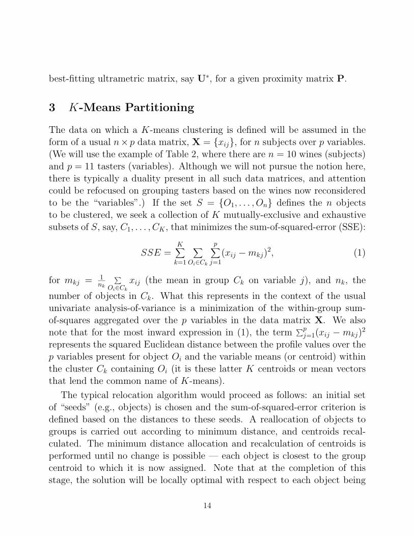
3 K-Means Partitioning

The data on which a K-means clustering is defined will be assumed in theform of a usual n× p data matrix, X = {xij}, for n subjects over p variables.(We will use the example of Table 2, where there are n = 10 wines (subjects)and p = 11 tasters (variables). Although we will not pursue the notion here,there is typically a duality present in all such data matrices, and attentioncould be refocused on grouping tasters based on the wines now reconsideredto be the “variables”.) If the set S = {O1, . . . , On} defines the n objectsto be clustered, we seek a collection of K mutually-exclusive and exhaustivesubsets of S, say, C1, . . . , CK , that minimizes the sum-of-squared-error (SSE):

SSE =K∑

k=1

∑

Oi∈Ck

p∑

j=1(xij −mkj)

2, (1)

for mkj = 1nk

∑Oi∈Ck

xij (the mean in group Ck on variable j), and nk, the

number of objects in Ck. What this represents in the context of the usualunivariate analysis-of-variance is a minimization of the within-group sum-of-squares aggregated over the p variables in the data matrix X. We alsonote that for the most inward expression in (1), the term

∑pj=1(xij − mkj)

2

represents the squared Euclidean distance between the profile values over thep variables present for object Oi and the variable means (or centroid) withinthe cluster Ck containing Oi (it is these latter K centroids or mean vectorsthat lend the common name of K-means).

The typical relocation algorithm would proceed as follows: an initial setof “seeds” (e.g., objects) is chosen and the sum-of-squared-error criterion isdefined based on the distances to these seeds. A reallocation of objects togroups is carried out according to minimum distance, and centroids recal-culated. The minimum distance allocation and recalculation of centroids isperformed until no change is possible — each object is closest to the groupcentroid to which it is now assigned. Note that at the completion of thisstage, the solution will be locally optimal with respect to each object being

14

closest to its group centroid. A final check can be made to determine if anysingle-object reallocations will reduce the sum-of-squared-error any further;at the completion of this stage, the solution will be locally optimal withrespect to (1).

We present a verbatim MATLAB session below in which we ask for twoto four clusters for the wines using the kmeans routine from the StatisticalToolbox on the cabernet_taste data matrix from Table 2. We choose one-hundred random starts (‘replicates’,100) by picking two to four objectsat random to serve as the initial seeds (‘start’,‘sample’). Two local op-tima were found for the choice of two clusters, but only one for three. Thecontrol phrase (‘maxiter’,1000) increases the allowable number of itera-tions; (‘display’,‘final’) controls printing the end results for each of thehundred replications; most of this latter output is suppressed to save spaceand replaced by ... ). The results actually displayed for each number ofchosen clusters are the best obtained over the hundred replications with idx

indicating cluster membership for the n objects; c contains the cluster cen-troids; sumd gives the within-cluster sum of object-to-centroid distances (sowhen the entries are summed, the objective function in (1) is generated); dincludes all the distances between each object and each centroid.

>> load cabernet_taste.dat

>> cabernet_taste

cabernet_taste =

14.0000 15.0000 10.0000 14.0000 15.0000 16.0000 14.0000 14.0000 13.0000 16.5000 14.0000

16.0000 14.0000 15.0000 15.0000 12.0000 16.0000 12.0000 14.0000 11.0000 16.0000 14.0000

12.0000 16.0000 11.0000 14.0000 12.0000 17.0000 14.0000 14.0000 14.0000 11.0000 15.0000

17.0000 15.0000 12.0000 12.0000 12.0000 13.5000 10.0000 8.0000 14.0000 17.0000 15.0000

13.0000 9.0000 12.0000 16.0000 7.0000 7.0000 12.0000 14.0000 17.0000 15.5000 11.0000

10.0000 10.0000 10.0000 14.0000 12.0000 11.0000 12.0000 12.0000 12.0000 8.0000 12.0000

12.0000 7.0000 11.5000 17.0000 2.0000 8.0000 10.0000 13.0000 15.0000 10.0000 9.0000

14.0000 5.0000 11.0000 13.0000 2.0000 9.0000 10.0000 11.0000 13.0000 16.5000 7.0000

5.0000 12.0000 8.0000 9.0000 13.0000 9.5000 14.0000 9.0000 12.0000 3.0000 13.0000

7.0000 7.0000 15.0000 15.0000 5.0000 9.0000 8.0000 13.0000 14.0000 6.0000 7.0000

>> [idx,c,sumd,d] = kmeans(cabernet_taste,2,’start’,’sample’,’replicates’,100,’maxiter’,1000,’display’,’final’)

2 iterations, total sum of distances = 633.208

3 iterations, total sum of distances = 633.063 ...

idx =

2

2

2

15

2

1

2

1

1

2

1

c =

11.5000 7.0000 12.3750 15.2500 4.0000 8.2500 10.0000 12.7500 14.7500 12.0000 8.5000

12.3333 13.6667 11.0000 13.0000 12.6667 13.8333 12.6667 11.8333 12.6667 11.9167 13.8333

sumd =

181.1875

451.8750

d =

329.6406 44.3125

266.1406 63.3125

286.6406 27.4792

286.8906 76.8958

46.6406 155.8125

130.3906 48.9792

12.5156 249.5625

50.3906 290.6458

346.8906 190.8958

71.6406 281.6458

_______________________________________________________________________________________________________________



idx =

1

1

1

1

2

3

2

2

3

2

c =

14.7500 15.0000 12.0000 13.7500 12.7500 15.6250 12.5000 12.5000 13.0000 15.1250 14.5000

11.5000 7.0000 12.3750 15.2500 4.0000 8.2500 10.0000 12.7500 14.7500 12.0000 8.5000

7.5000 11.0000 9.0000 11.5000 12.5000 10.2500 13.0000 10.5000 12.0000 5.5000 12.5000

sumd =

117.1250

16

181.1875

50.1250

d =

16.4688 329.6406 242.3125

21.3438 266.1406 289.5625

34.8438 286.6406 155.0625

44.4688 286.8906 284.0625

182.4688 46.6406 244.8125

132.0938 130.3906 25.0625

323.0938 12.5156 244.8125

328.2188 50.3906 357.8125

344.9688 346.8906 25.0625

399.5938 71.6406 188.0625

_______________________________________________________________________________________________________________






idx =

4

4

4

4

2

3

2

2

3

1

c =

7.0000 7.0000 15.0000 15.0000 5.0000 9.0000 8.0000 13.0000 14.0000 6.0000 7.0000

13.0000 7.0000 11.5000 15.3333 3.6667 8.0000 10.6667 12.6667 15.0000 14.0000 9.0000

7.5000 11.0000 9.0000 11.5000 12.5000 10.2500 13.0000 10.5000 12.0000 5.5000 12.5000

14.7500 15.0000 12.0000 13.7500 12.7500 15.6250 12.5000 12.5000 13.0000 15.1250 14.5000

sumd =

0

85.6667

50.1250

117.1250

d =

485.2500 309.6111 242.3125 16.4688

403.0000 252.3611 289.5625 21.3438

362.0000 293.3611 155.0625 34.8438

17

465.2500 259.2778 284.0625 44.4688

190.2500 30.6111 244.8125 182.4688

147.0000 156.6944 25.0625 132.0938

76.2500 23.1111 244.8125 323.0938

201.2500 31.9444 357.8125 328.2188

279.2500 401.2778 25.0625 344.9688

0 127.3611 188.0625 399.5938

The separation of the wines into three groups (having objective functionvalue of 348.438) results in the clusters: {A,B, C,D}, {E, G, H, J}, {F, I}.Here, {A,B, C, D} represents the four absolute “best” wines with the soleU.S. entry of Stag’s Leap (A) in this mix; {E, G,H, J} are four wines that arerated at the absolute bottom (consistently) for four of the tasters (2,5,6,11)and are all U.S. products; the last class, {F, I}, includes one French and oneU.S. label with more variable ratings over the judges. This latter group alsocoalesces with the best group when only two clusters are sought. From anonchauvinistic perspective, the presence of the single U.S. offering of Stag’sLeap in the “best” group of four (within the three-class solution) does notsay very strongly to us that the U.S. has somehow “won”.

3.1 K-Means and Matrix Partitioning

The most inward expression in (1),

∑

Oi∈Ck

p∑

j=1(xij −mkj)

2, (2)

can be interpreted as the sum of the squared Euclidean distances betweenevery object in Ck and the centroid for this cluster. These sums are ag-gregated, in turn, over k (from 1 to K) to obtain the sum-of-squared-errorcriterion that we attempt to minimize in K-means clustering by the judiciouschoice of C1, . . . , CK . Alternatively, the expression in (2) can be re-expressedas

1

2nk

∑

Oi,Oi′∈Ck

p∑

j=1(xij − xi′j)

2, (3)

or a quantity equal to the sum of the squared Euclidean distances betweenall object pairs in Ck divided by twice the number of objects, nk, in Ck. Ifwe define the proximity, pii′, between any two objects, Oi and Oi′, over the p

18

variables as the squared Euclidean distance, then (3) could be rewritten as

1

2nk

∑

Oi,Oi′∈Ck

pii′.

Or, consider the proximity matrix P = {pii′} and for any clustering, C1, . . . , CK ,the proximity matrix can be schematically represented as

C1 · · · Ck · · · CK

C1 P11 · · · P1k · · · P1K...

... · · · ... · · · ...Ck Pk1 · · · Pkk · · · PkK...

... · · · ... · · · ...CK PK1 · · · PKk · · · PKK

where the objects in S have been reordered so each cluster Ck represents acontiguous segment of (ordered objects) and Pkk′ is the nk×nk′ collection ofproximities between the objects in Ck and Ck′. In short, the sum-of-squared-error criterion is merely the sum of proximities in Pkk weighted by 1

2nkand

aggregated over k from 1 to K (i.e., the sum of the main diagonal blocks ofP). In fact, any clustering evaluated with the sum-of-squared-error criterioncould be represented by such a structure defined with a reordered proximitymatrix having its rows and columns grouped to contain the contiguous objectsin C1, . . . , CK .

To give an example of this kind of proximity matrix for our cabernetexample, the squared Euclidean distance matrix among the wines is given inTable 4 with the row and column objects reordered to conform to the three-group K-means clustering. The expression in (3) in relation to Table 4 wouldbe given as

1

2n1

∑

Oi,Oi′∈C1

pii′ +1

2n2

∑

Oi,Oi′∈C2

pii′ +1

2n3

∑

Oi,Oi′∈C3

pii′ =

1

2(4)(937.00) +

1

2(4)(1449.50) +

1

2(2)(200.50) =

19

ClassWine

C1/A C1/B C1/C C1/D C2/E C2/G C2/H C2/J C3/F C3/IC1/A .00 48.25 48.25 86.50 220.00 400.50 394.00 485.25 160.25 374.50C1/B 48.25 .00 77.00 77.25 195.25 327.25 320.25 403.00 176.00 453.25C1/C 48.25 77.00 .00 131.25 229.25 326.25 410.25 362.00 107.00 253.25C1/D 86.50 77.25 131.25 .00 202.50 355.50 305.50 465.25 202.25 416.00C2/E 220.00 195.25 229.25 202.50 .00 75.50 102.00 190.25 145.25 394.50C2/G 400.50 327.25 326.25 355.50 75.50 .00 79.50 76.25 160.25 379.50C2/H 394.00 320.25 410.25 305.50 102.00 79.50 .00 201.25 250.25 515.50C2/J 485.25 403.00 362.00 465.25 190.25 76.25 201.25 .00 147.00 279.25C3/F 160.25 176.00 107.00 202.25 145.25 160.25 250.25 147.00 .00 100.25C3/I 374.50 453.25 253.25 416.00 394.50 379.50 515.50 279.25 100.25 .00

Table 4: Squared Euclidean Distances Among Ten Cabernets.

117.1250 + 181.1875 + 50.1250 = 348.438

This is the same objective function value from (1) reported in the verbatimMATLAB output.

4 Beyond the Basics: Extensions of Hierarchical Clus-

tering and K-Means Partitioning

A brief introduction to the two dominant tasks of hierarchical clustering andK-means partitioning have been provided in the previous two sections. Here,several extensions of these ideas will be discussed to make the analysis tech-niques generally more useful to the user. In contrast to earlier sections wherethe cited MATLAB routines were already part of the Statistics Toolbox, theM-files from this section on are available (open-source) from the authors’ website:

http://cda.psych.uiuc.edu/clusteranalysis_mfiles

We provide the help “header” files for all of these M-files in an Appendix Ato this chapter; these should be generally helpful in explaining both syntaxand usage.

The four subsections below deal successively with the following topics (withexamples to follow thereafter):

20

(a) The hierarchical clustering task can be reformulated as locating a best-fitting ultrametric, say U∗ = {u∗ij}, to the given proximity matrix, P, suchthat the least-squares criterion

∑

i<j

(pij − u∗ij)2 ,

is minimized. The approach can either be confirmatory (in which we lookfor the best-fitting ultrametric defined by some monotone transformation ofthe n − 1 values making up a fixed ultrametric), or exploratory (where wemerely look for the best-fitting ultrametric without any prior constraint asto its form). In both cases, a convenient normalized loss measure is given bythe variance-accounted-for (VAF):

VAF = 1−∑

i<j(pij − u∗ij)2

∑i<j(pij − p)2 ,

where p is the average off-diagonal proximity value in P. This is directlycomparable to the usual VAF measure familiar from multiple regression.

(b) In identifying a best-fitting ultrametric and displaying it subsequentlythrough a dendrogram, there is a degree of arbitrariness in how the terminalnodes are ordered. If we treat the dendrogram as a “mobile” and allow theinternal nodes to act as universal joints with freedom of 360◦ degree rotation,there are 2n−1 equivalent orderings of the terminal nodes (in our example, 28 is256), and none is preferred a priori. To impose some meaning on the terminalnode ordering, we provide two routines that either impose a given orderingor look for a “best” one that could be used for display in the exploratoryidentification of a best-fitting ultrametric. These routines rely on a prelim-inary identification of a least-squares best-fitting anti-Robinson matrix (ananti-Robinson (AR) matrix is one in which the entries never decrease whenmoving within the rows or columns away from the main diagonal entries).Treating the fitted AR matrix as the collection of “proximities” in their ownright, the process of finding a best-fitting ultrametric is then carried out,producing a dendrogram that is consistently displayable with respect to theconstraining order. In effect, we are combining the two (somewhat) differenttasks of hierarchical clustering and the seriation of an object set by reordering

21

the rows and columns of P to display as closely as possible, a particularlyappealing AR gradient in its entries.

(c) In observing that the K-means criterion could be reinterpreted througha proximity matrix defined by squared Euclidean distances, it was also notedthat the clusters could be represented as contiguous segments of orderedobjects in a reordered proximity matrix. We exploit this connection byrephrasing the search for the better (in the sense of hopefully being moresubstantively interpretable) partitions by imposing a preliminary order onthe squared Euclidean proximity matrix; then, for a given number of clus-ters, a (globally) optimal subdivision is found based on the K-means criterion(the M-file that carries this out is an implementation of an order-constraineddynamic programming (DP) routine that can handle a very large numberof objects with guaranteed (order-constrained) optimality for the traditionalK-means criterion). It appears that this tandem strategy of finding an orderfirst and then carrying out a K-means subdivision, does well in its genera-tion of substantively interpretable partitions. It’s as if we are simultaneouslyoptimizing two objective functions — one that provides a typically good ap-proximate AR ordering for the squared Euclidean distances (an AR orderingthat, in fact, might be interpretable more-or-less “as is”), and a second thatis not prone to the local optimum problem plaguing all K-means iterativemethods because it is based on a DP strategy guaranteeing global optimality(albeit within an order-constrained context).

(d) The idea of providing an optimal mechanism for subdividing an order-constrained proximity matrix (and not one just based on squared Euclideandistances), gives a natural means for generalizing the usual (agglomerative)hierarchical clustering methods, such as complete- or average-link. Defininga good preliminary constraining order for the proximity matrix, an optimiza-tion routine (based on DP) is implemented that will give optimal partitionsinto 2 to n − 1 classes respecting the preliminary order (having classes con-taining objects contiguous with respect to it), and minimizing the maximumsuch measure obtained over the classes making up the partitions (the max-imum proximity [or diameter] within a class for the complete-link criterion;the average of the proximities within a class for the average-link criterion).The “minimum of the maximum” is used because otherwise a tendency will

22

exist to produce just one large class for each optimal partition; also, thisseems a closer analogue to agglomerative hierarchical clustering when we tryto minimize a maximum as each partition is constructed from the proceedingone. Stated alternatively, the best single partition optimization analogue tohierarchical clustering, with the latter’s myopic process and greedy “best itcan do” at each next level, would be the optimization goal of minimizing themaximum subset measure over the classes of a partition. In the case of ourK-means interpretation in (c), a simple sum over the classes can be optimizedthat does not generally lead to the “one big class” triviality, apparently be-cause of the divisions by twice the number of objects within each class in thespecific loss function used in the optimization.

4.1 A Useful Utility: Obtaining a Constraining Order

In implementing an order-constrained K-means clustering strategy, an ap-propriate initial ordering must be generated to constrain the clustering inthe first place. Although many strategies might be considered, a particularlypowerful one appears definable through what is called the quadratic assign-ment (QA) task and a collection of local-improvement optimization heuristics.As typically defined, a QA problem involves two n × n matrices, A = {aij}and T = {tij}, and we seek a permutation to maximize the cross-productstatistic

Γ(ρ) =∑

i6=j

aρ(i)ρ(j)tij . (4)

The notation {aρ(i)ρ(j)} implies a reordering (by the permutation ρ(·)) of therows and simultaneously the columns of A so that the rows (and columns)now appear in the order ρ(1) Â ρ(2) Â · · · Â ρ(n). For our purposes, thefirst matrix A could be identified with the proximity matrix P containingsquared Euclidean distances between the subject profiles over the p variables;the second matrix contains a target defined by a set of locations equally-spaced along a line, i.e., T = {|j − i|} for 1 ≤ i, j ≤ n. (More generally,P could be any proximity matrix having a dissimilarity interpretation; useof the resulting identified permutation, for example, would be one way ofimplementing an order-constrained DP proximity matrix subdivision.)

23

In attempting to find ρ to maximize Γ(ρ), we try to reorganize the prox-imity matrix as Pρ = {pρ(i)ρ(j)}, to show the same pattern, more or less, asthe fixed target T; equivalently, we maximize the usual Pearson product-moment correlation between the off-diagonal entries in T and Pρ. Anotherway of rephrasing this search is to say that we seek a permutation ρ that pro-vides a structure as “close” as possible to an AR form for Pρ, i.e., the degreeto which the entries in Pρ, moving away from the main diagonal in eitherdirection never decrease (and usually increase); this is exactly the patternexhibited by the equally-spaced target matrix T. In our order-constrainedK-means application, once the proximity matrix is so reordered by ρ, welook for a K-means clustering result that respects the order generating the“as close as we can get to an AR” patterning for the row/column permutedmatrix.

The type of heuristic optimization strategy we use for the QA task imple-ments simple object interchange/rearrangement operations. Based on givenmatrices A and T, and beginning with some permutation (possibly chosenat random), local interchanges and rearrangements of a particular type areimplemented until no improvement in the index can be made. By repeat-edly initializing such a process randomly, a distribution over a set of localoptima can be achieved. Three different classes of local operations are usedin the M-file, order.m: (i) the pairwise interchanges of objects in the currentpermutation defining the row and column order of the data matrix A. Allpossible such interchanges are generated and considered in turn, and when-ever an increase in the cross-product index would result from a particularinterchange, it is made immediately. The process continues until the currentpermutation cannot be improved upon by any such pairwise object inter-change. The procedure then proceeds to (ii): the local operations consideredare all reinsertions of from 1 to kblock (which is less than n and set by theuser) consecutive objects somewhere in the permutation defining the currentrow and column order of the data matrix. When no further improvementcan be made, we move to (iii): the local operations are now all possible rota-tions (or inversions) of from 2 to kblock consecutive objects in the currentrow/column order of the data matrix. (We suggest a use of kblock equal to 3as a reasonable compromise between the extensiveness of local search, speed

24

of execution, and quality of solution.) The three collections of local changesare revisited (in order) until no alteration is possible in the final permutationobtained.

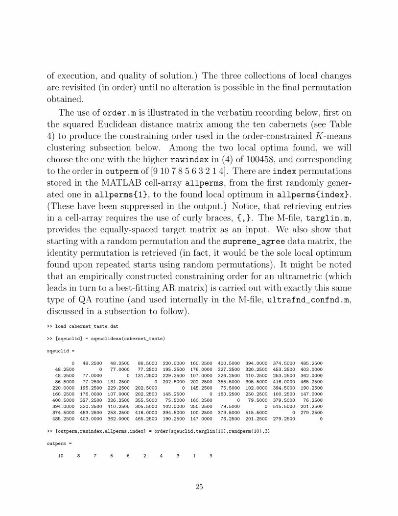
The use of order.m is illustrated in the verbatim recording below, first onthe squared Euclidean distance matrix among the ten cabernets (see Table4) to produce the constraining order used in the order-constrained K-meansclustering subsection below. Among the two local optima found, we willchoose the one with the higher rawindex in (4) of 100458, and correspondingto the order in outperm of [9 10 7 8 5 6 3 2 1 4]. There are index permutationsstored in the MATLAB cell-array allperms, from the first randomly gener-ated one in allperms{1}, to the found local optimum in allperms{index}.(These have been suppressed in the output.) Notice, that retrieving entriesin a cell-array requires the use of curly braces, {,}. The M-file, targlin.m,provides the equally-spaced target matrix as an input. We also show thatstarting with a random permutation and the supreme_agree data matrix, theidentity permutation is retrieved (in fact, it would be the sole local optimumfound upon repeated starts using random permutations). It might be notedthat an empirically constructed constraining order for an ultrametric (whichleads in turn to a best-fitting AR matrix) is carried out with exactly this sametype of QA routine (and used internally in the M-file, ultrafnd_confnd.m,discussed in a subsection to follow).

>> load cabernet_taste.dat

>> [sqeuclid] = sqeuclidean(cabernet_taste)

sqeuclid =

0 48.2500 48.2500 86.5000 220.0000 160.2500 400.5000 394.0000 374.5000 485.2500

48.2500 0 77.0000 77.2500 195.2500 176.0000 327.2500 320.2500 453.2500 403.0000

48.2500 77.0000 0 131.2500 229.2500 107.0000 326.2500 410.2500 253.2500 362.0000

86.5000 77.2500 131.2500 0 202.5000 202.2500 355.5000 305.5000 416.0000 465.2500

220.0000 195.2500 229.2500 202.5000 0 145.2500 75.5000 102.0000 394.5000 190.2500

160.2500 176.0000 107.0000 202.2500 145.2500 0 160.2500 250.2500 100.2500 147.0000

400.5000 327.2500 326.2500 355.5000 75.5000 160.2500 0 79.5000 379.5000 76.2500

394.0000 320.2500 410.2500 305.5000 102.0000 250.2500 79.5000 0 515.5000 201.2500

374.5000 453.2500 253.2500 416.0000 394.5000 100.2500 379.5000 515.5000 0 279.2500

485.2500 403.0000 362.0000 465.2500 190.2500 147.0000 76.2500 201.2500 279.2500 0

>> [outperm,rawindex,allperms,index] = order(sqeuclid,targlin(10),randperm(10),3)

outperm =

10 8 7 5 6 2 4 3 1 9

25

rawindex =

100333

index =

11

>> [outperm,rawindex,allperms,index] = order(sqeuclid,targlin(10),randperm(10),3)

outperm =

9 10 7 8 5 6 3 2 1 4

rawindex =

100458

index =

18


>> [outperm,rawindex,allperms,index] = order(supreme_agree,targlin(9),randperm(9),3)

outperm =

1 2 3 4 5 6 7 8 9

rawindex =

145.1200

index =

19

4.2 The Least-Squares Finding and Fitting of Ultrametrics

A least-squares approach to identifying good ultrametrics is governed bytwo M-files, ultrafit.m (for confirmatory fitting) and ultrafnd.m (for ex-ploratory finding). The syntaxes for both are as follows:

[fit,vaf] = ultrafit(prox,targ)

[find,vaf] = ultrafnd(prox,inperm)

26

Here, prox refers to the input proximity matrix; targ is of the same size asprox, with the same row and column order, and contains values conforming toan ultrametric (e.g., the complete-link ultrametric values of Table 3); inpermis an input permutation of the n objects that controls the heuristic searchprocess for identifying the ultrametric constraints to impose (this is usuallygiven by the built-in random permutation randperm(n), where n is replacedby the actual number of objects; different random starts can be tried inthe heuristic search to investigate the distribution of possible local optima);fit and find refer to the confirmatory or exploratory identified ultrametricmatrices, respectively, with the common meaning of variance-accounted-forgiven to vaf.

A MATLAB session using these two functions is reproduced below. Thecomplete-link target ultrametric matrix, sc_completelink_target, with thesame row and column ordering as supreme_agree induces a least-squares con-firmatory fitted matrix having VAF of 73.69%. The monotonic function, sayf(·), between the values of the fitted and input target matrices can be given asfollows: f(.21) = .21; f(.22) = .22; f(.23) = .23; f(.29) = .2850; f(.33) =.31; f(.38) = .3633; f(.46) = .4017; f(.86) = .6405. Interestingly, an ex-ploratory use of ultrafnd.m produces exactly this same result; also, thereappears to be only this one local optimum identifiable over many randomstarts (these results are not explicitly reported here but can be replicated eas-ily by the reader. Thus, at least for this particular data set, the complete-linkmethod produces the optimal [least-squares] branching structure as verifiedover repeated random initializations for ultrafnd.m).

>> load sc_completelink_target.dat

>> sc_completelink_target

sc_completelink_target =

0 0.3800 0.3800 0.3800 0.8600 0.8600 0.8600 0.8600 0.8600

0.3800 0 0.2900 0.2900 0.8600 0.8600 0.8600 0.8600 0.8600

0.3800 0.2900 0 0.2200 0.8600 0.8600 0.8600 0.8600 0.8600

0.3800 0.2900 0.2200 0 0.8600 0.8600 0.8600 0.8600 0.8600

0.8600 0.8600 0.8600 0.8600 0 0.3300 0.3300 0.4600 0.4600

0.8600 0.8600 0.8600 0.8600 0.3300 0 0.2300 0.4600 0.4600

0.8600 0.8600 0.8600 0.8600 0.3300 0.2300 0 0.4600 0.4600

0.8600 0.8600 0.8600 0.8600 0.4600 0.4600 0.4600 0 0.2100

0.8600 0.8600 0.8600 0.8600 0.4600 0.4600 0.4600 0.2100 0

>> load supreme_agree.dat;

27

>> [fit,vaf] = ultrafit(supreme_agree,sc_completelink_target)

fit =

0 0.3633 0.3633 0.3633 0.6405 0.6405 0.6405 0.6405 0.6405

0.3633 0 0.2850 0.2850 0.6405 0.6405 0.6405 0.6405 0.6405

0.3633 0.2850 0 0.2200 0.6405 0.6405 0.6405 0.6405 0.6405

0.3633 0.2850 0.2200 0 0.6405 0.6405 0.6405 0.6405 0.6405

0.6405 0.6405 0.6405 0.6405 0 0.3100 0.3100 0.4017 0.4017

0.6405 0.6405 0.6405 0.6405 0.3100 0 0.2300 0.4017 0.4017

0.6405 0.6405 0.6405 0.6405 0.3100 0.2300 0 0.4017 0.4017

0.6405 0.6405 0.6405 0.6405 0.4017 0.4017 0.4017 0 0.2100

0.6405 0.6405 0.6405 0.6405 0.4017 0.4017 0.4017 0.2100 0

vaf =

0.7369

>> [find,vaf] = ultrafnd(supreme_agree,randperm(9))

find =

0 0.3633 0.3633 0.3633 0.6405 0.6405 0.6405 0.6405 0.6405

0.3633 0 0.2850 0.2850 0.6405 0.6405 0.6405 0.6405 0.6405

0.3633 0.2850 0 0.2200 0.6405 0.6405 0.6405 0.6405 0.6405

0.3633 0.2850 0.2200 0 0.6405 0.6405 0.6405 0.6405 0.6405

0.6405 0.6405 0.6405 0.6405 0 0.3100 0.3100 0.4017 0.4017

0.6405 0.6405 0.6405 0.6405 0.3100 0 0.2300 0.4017 0.4017

0.6405 0.6405 0.6405 0.6405 0.3100 0.2300 0 0.4017 0.4017

0.6405 0.6405 0.6405 0.6405 0.4017 0.4017 0.4017 0 0.2100

0.6405 0.6405 0.6405 0.6405 0.4017 0.4017 0.4017 0.2100 0

vaf =

0.7369

As noted earlier, the ultrametric fitted values obtained through least-squares are actually average proximities of a similar type used in average-linkhierarchical clustering. This should not be surprising given that any sum-of-squared deviations of a set of observations from a common value is minimizedwhen that common value is the arithmetic mean. For the monotonic functionreported above, the various values are the average proximities between thesubsets united in forming the partition hierarchy:

.21 = .21; .22 = .22; .23 = .23; .2850 = (.28 + .29)/2;

.31 = (.33 + .29)/2; .3633 = (.38 + .34 + .37)/3;

.4017 = (.46 + .42 + .34 + .46 + .41 + .32)/6;

.6405 = (.67 + .64 + .75 + .86 + .85 + .45 + .53 + .57 + .75 + .76 +

.53 + .51 + .57 + .72 + .74 + .45 + .50 + .56 + .69 + .71)/20.

28

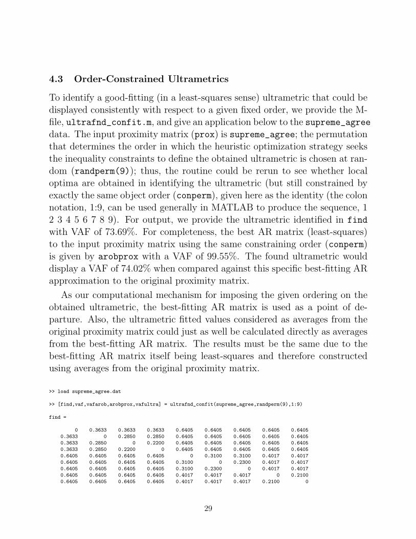
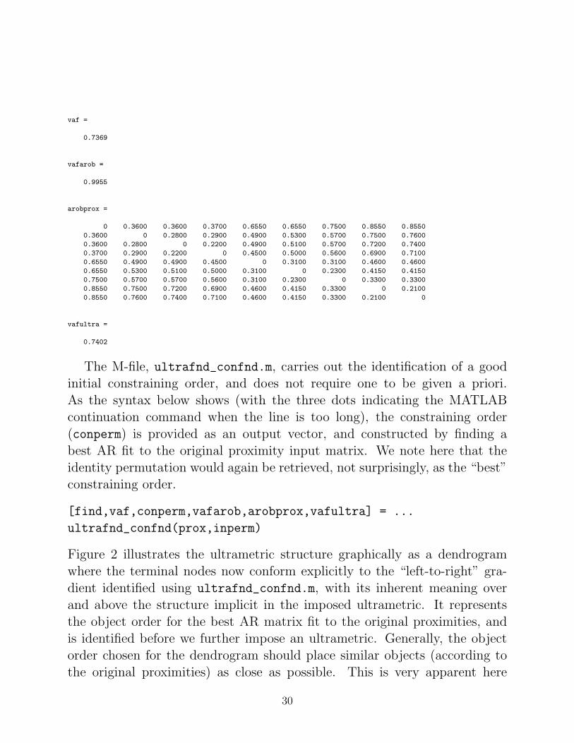
4.3 Order-Constrained Ultrametrics

To identify a good-fitting (in a least-squares sense) ultrametric that could bedisplayed consistently with respect to a given fixed order, we provide the M-file, ultrafnd_confit.m, and give an application below to the supreme_agreedata. The input proximity matrix (prox) is supreme_agree; the permutationthat determines the order in which the heuristic optimization strategy seeksthe inequality constraints to define the obtained ultrametric is chosen at ran-dom (randperm(9)); thus, the routine could be rerun to see whether localoptima are obtained in identifying the ultrametric (but still constrained byexactly the same object order (conperm), given here as the identity (the colonnotation, 1:9, can be used generally in MATLAB to produce the sequence, 12 3 4 5 6 7 8 9). For output, we provide the ultrametric identified in find

with VAF of 73.69%. For completeness, the best AR matrix (least-squares)to the input proximity matrix using the same constraining order (conperm)is given by arobprox with a VAF of 99.55%. The found ultrametric woulddisplay a VAF of 74.02% when compared against this specific best-fitting ARapproximation to the original proximity matrix.

As our computational mechanism for imposing the given ordering on theobtained ultrametric, the best-fitting AR matrix is used as a point of de-parture. Also, the ultrametric fitted values considered as averages from theoriginal proximity matrix could just as well be calculated directly as averagesfrom the best-fitting AR matrix. The results must be the same due to thebest-fitting AR matrix itself being least-squares and therefore constructedusing averages from the original proximity matrix.


>> [find,vaf,vafarob,arobprox,vafultra] = ultrafnd_confit(supreme_agree,randperm(9),1:9)

find =

0 0.3633 0.3633 0.3633 0.6405 0.6405 0.6405 0.6405 0.6405

0.3633 0 0.2850 0.2850 0.6405 0.6405 0.6405 0.6405 0.6405

0.3633 0.2850 0 0.2200 0.6405 0.6405 0.6405 0.6405 0.6405

0.3633 0.2850 0.2200 0 0.6405 0.6405 0.6405 0.6405 0.6405

0.6405 0.6405 0.6405 0.6405 0 0.3100 0.3100 0.4017 0.4017

0.6405 0.6405 0.6405 0.6405 0.3100 0 0.2300 0.4017 0.4017

0.6405 0.6405 0.6405 0.6405 0.3100 0.2300 0 0.4017 0.4017

0.6405 0.6405 0.6405 0.6405 0.4017 0.4017 0.4017 0 0.2100

0.6405 0.6405 0.6405 0.6405 0.4017 0.4017 0.4017 0.2100 0

29

vaf =

0.7369

vafarob =

0.9955

arobprox =

0 0.3600 0.3600 0.3700 0.6550 0.6550 0.7500 0.8550 0.8550

0.3600 0 0.2800 0.2900 0.4900 0.5300 0.5700 0.7500 0.7600

0.3600 0.2800 0 0.2200 0.4900 0.5100 0.5700 0.7200 0.7400

0.3700 0.2900 0.2200 0 0.4500 0.5000 0.5600 0.6900 0.7100

0.6550 0.4900 0.4900 0.4500 0 0.3100 0.3100 0.4600 0.4600

0.6550 0.5300 0.5100 0.5000 0.3100 0 0.2300 0.4150 0.4150

0.7500 0.5700 0.5700 0.5600 0.3100 0.2300 0 0.3300 0.3300

0.8550 0.7500 0.7200 0.6900 0.4600 0.4150 0.3300 0 0.2100

0.8550 0.7600 0.7400 0.7100 0.4600 0.4150 0.3300 0.2100 0

vafultra =

0.7402

The M-file, ultrafnd_confnd.m, carries out the identification of a goodinitial constraining order, and does not require one to be given a priori.As the syntax below shows (with the three dots indicating the MATLABcontinuation command when the line is too long), the constraining order(conperm) is provided as an output vector, and constructed by finding abest AR fit to the original proximity input matrix. We note here that theidentity permutation would again be retrieved, not surprisingly, as the “best”constraining order.

[find,vaf,conperm,vafarob,arobprox,vafultra] = ...

ultrafnd_confnd(prox,inperm)

Figure 2 illustrates the ultrametric structure graphically as a dendrogramwhere the terminal nodes now conform explicitly to the “left-to-right” gra-dient identified using ultrafnd_confnd.m, with its inherent meaning overand above the structure implicit in the imposed ultrametric. It representsthe object order for the best AR matrix fit to the original proximities, andis identified before we further impose an ultrametric. Generally, the objectorder chosen for the dendrogram should place similar objects (according tothe original proximities) as close as possible. This is very apparent here

30

where the particular (identity) constraining order imposed has an obviousmeaning. We note that Figure 2 is not drawn using the dendrogram routinefrom MATLAB because there is no convenient way in the latter to controlthe order of the terminal nodes (see Figure 1 as an example where one of the256 equivalent mobile orderings is chosen [rather arbitrarily] to display thejustices). Figure 2 was done “by hand” in the LATEX picture environmentwith an explicit left-to-right order imposed among the justices.

4.4 Order-Constrained K-Means Clustering

To illustrate how order-constrained K-means clustering might be implemented,we go back to the wine tasting data and adopt as a constraining order thepermutation [9 10 7 8 5 6 3 2 1 4] identified earlier through order.m. In theverbatim analysis below, it should be noted that an input matrix of

wineprox = sqeuclid([9 10 7 8 5 6 3 2 1 4],[9 10 7 8 5 6 3 2 1 4])

is used in partitionfnd_kmeans.m, which then induces the mandatory con-straining identity permutation for the input matrix. This also implies alabeling of the columns of the membership matrix of [9 10 7 8 5 6 3 2 1 4] or[I J G H E F C B A D]. Considering alternatives to the earlier K-means anal-ysis, it is interesting (and possibly substantively more meaningful) to notethat the two-group solution puts the best wines ({A,B,C,D}) versus the rest({E,F,G,H,I,J}) (and is actually the second local optima identified for K = 2with an objective function loss of 633.208). The four-group solution is veryinterpretable and defined by the best ({A,B,C,D}), the worst ({E,G,H,J}),and the two “odd-balls” in separate classes ({F} and {G}). Its loss value of298.300 is somewhat more than the least attainable of 252.917 (found for theless-than-pleasing subdivision, ({A,B,C,D},{E,G,H},{F,I},{J}).>> load cabernet_taste.dat

>> [sqeuclid] = sqeuclidean(cabernet_taste)

sqeuclid =

0 48.2500 48.2500 86.5000 220.0000 160.2500 400.5000 394.0000 374.5000 485.2500

48.2500 0 77.0000 77.2500 195.2500 176.0000 327.2500 320.2500 453.2500 403.0000

48.2500 77.0000 0 131.2500 229.2500 107.0000 326.2500 410.2500 253.2500 362.0000

86.5000 77.2500 131.2500 0 202.5000 202.2500 355.5000 305.5000 416.0000 465.2500

220.0000 195.2500 229.2500 202.5000 0 145.2500 75.5000 102.0000 394.5000 190.2500

31

Figure 2: A Dendrogram (Tree) Representation for the Ordered-Constrained UltrametricDescribed in the Text (Having VAF of 73.69%)

St Br Gi So Oc Ke Re Sc Th

i i i i i i i i i

y

y

y

y

y

y

y

~

-.21 -.22 -.23

-.29-.31

-.36

-.40

-.64

32

160.2500 176.0000 107.0000 202.2500 145.2500 0 160.2500 250.2500 100.2500 147.0000

400.5000 327.2500 326.2500 355.5000 75.5000 160.2500 0 79.5000 379.5000 76.2500

394.0000 320.2500 410.2500 305.5000 102.0000 250.2500 79.5000 0 515.5000 201.2500

374.5000 453.2500 253.2500 416.0000 394.5000 100.2500 379.5000 515.5000 0 279.2500

485.2500 403.0000 362.0000 465.2500 190.2500 147.0000 76.2500 201.2500 279.2500 0

>> wineprox = sqeuclid([9 10 7 8 5 6 3 2 1 4],[9 10 7 8 5 6 3 2 1 4])

wineprox =

0 279.2500 379.5000 515.5000 394.5000 100.2500 253.2500 453.2500 374.5000 416.0000

279.2500 0 76.2500 201.2500 190.2500 147.0000 362.0000 403.0000 485.2500 465.2500

379.5000 76.2500 0 79.5000 75.5000 160.2500 326.2500 327.2500 400.5000 355.5000

515.5000 201.2500 79.5000 0 102.0000 250.2500 410.2500 320.2500 394.0000 305.5000

394.5000 190.2500 75.5000 102.0000 0 145.2500 229.2500 195.2500 220.0000 202.5000

100.2500 147.0000 160.2500 250.2500 145.2500 0 107.0000 176.0000 160.2500 202.2500

253.2500 362.0000 326.2500 410.2500 229.2500 107.0000 0 77.0000 48.2500 131.2500

453.2500 403.0000 327.2500 320.2500 195.2500 176.0000 77.0000 0 48.2500 77.2500

374.5000 485.2500 400.5000 394.0000 220.0000 160.2500 48.2500 48.2500 0 86.5000

416.0000 465.2500 355.5000 305.5000 202.5000 202.2500 131.2500 77.2500 86.5000 0

>> [membership,objectives] = partitionfnd_kmeans(wineprox)

membership =

1 1 1 1 1 1 1 1 1 1

2 2 2 2 2 2 1 1 1 1

3 2 2 2 2 2 1 1 1 1

4 3 3 3 3 2 1 1 1 1

5 4 3 3 3 2 1 1 1 1

6 5 4 4 4 3 2 2 2 1

7 6 6 5 4 3 2 2 2 1

8 7 6 5 4 3 2 2 2 1

9 8 7 6 5 4 3 2 2 1

10 9 8 7 6 5 4 3 2 1

objectives =

1.0e+003 *

1.1110

0.6332

0.4026

0.2983

0.2028

0.1435

0.0960

0.0578

0.0241

0

4.5 Order-Constrained Partitioning

Given the broad characterization of the properties of an ultrametric describedearlier, the generalization to be mentioned within this subsection rests onmerely altering the type of partition allowed in the sequence, P0,P1, . . . ,Pn−1.

33

Specifically, we will use an object order assumed without loss of generalityto be the identity permutation, O1 ≺ · · · ≺ On, and a collection of partitionswith fewer and fewer classes consistent with this order by requiring the classeswithin each partition to contain contiguous objects. When necessary, and ifan input constraining order is given by, say, inperm, that is not the identity,we merely use the input matrix, prox_input = prox(inperm,inperm); theidentity permutation then constrains the analysis automatically, although ineffect the constraint is given by inperm which also labels the columns ofmembership.

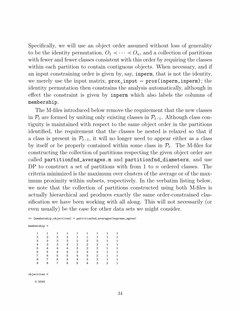
The M-files introduced below remove the requirement that the new classesin Pt are formed by uniting only existing classes in Pt−1. Although class con-tiguity is maintained with respect to the same object order in the partitionsidentified, the requirement that the classes be nested is relaxed so that ifa class is present in Pt−1, it will no longer need to appear either as a classby itself or be properly contained within some class in Pt. The M-files forconstructing the collection of partitions respecting the given object order arecalled partitionfnd_averages.m and partitionfnd_diameters, and useDP to construct a set of partitions with from 1 to n ordered classes. Thecriteria minimized is the maximum over clusters of the average or of the max-imum proximity within subsets, respectively. In the verbatim listing below,we note that the collection of partitions constructed using both M-files isactually hierarchical and produces exactly the same order-constrained clas-sification we have been working with all along. This will not necessarily (oreven usually) be the case for other data sets we might consider.

>> [membership,objectives] = partitionfnd_averages(supreme_agree)

membership =

1 1 1 1 1 1 1 1 1

2 2 2 2 1 1 1 1 1

3 3 3 3 2 2 2 1 1

4 3 3 3 2 2 2 1 1

5 4 4 4 3 2 2 1 1

6 5 4 4 3 2 2 1 1

7 6 5 5 4 3 2 1 1

8 7 6 5 4 3 2 1 1

9 8 7 6 5 4 3 2 1

objectives =

0.5044

34

0.3470

0.3133

0.2833

0.2633

0.2300

0.2200

0.2100

0

>> [membership,objectives] = partitionfnd_diameters(supreme_agree)

membership =

1 1 1 1 1 1 1 1 1

2 2 2 2 1 1 1 1 1

3 3 3 3 2 2 1 1 1

4 3 3 3 2 2 2 1 1

5 4 4 4 3 2 2 1 1

6 5 4 4 3 2 2 1 1

7 6 5 5 4 3 2 1 1

8 7 6 5 4 3 2 1 1

9 8 7 6 5 4 3 2 1

objectives =

0.8600

0.4600

0.3800

0.3300

0.2900

0.2300

0.2200

0.2100

0

5 An Alternative and Generalizable View of Ultramet-

ric Matrix Decomposition

A general mechanism exists for decomposing any ultrametric matrix U intoa (nonnegatively) weighted sum of dichotomous (0/1) matrices, each repre-senting one of the partitions of the hierarchy, P0, . . . ,Pn−2, induced by U(note that the conjoint partition is explicitly excluded in these expressions

for the numerical reason we allude to below). Specifically, if Pt = {p(t)ij }, for

0 ≤ t ≤ n−2, is an n×n symmetric (0/1) dissimilarity matrix corresponding

to Pt in which an entry p(t)ij is 0 if Oi and Oj belong to the same class in Pt and

otherwise equal to 1, then for some collection of suitably chosen nonnegativeweights, α0, α1, . . . , αn−2,

U =n−2∑

t=0αtPt .

35

Generally, the nonnegative weights, α0, α1, . . . , αn−2, are given by the (dif-ferences in) partition increments that calibrate the vertical axis of the den-drogram. Moreover, because the ultrametric represented by Figure 2 wasgenerated by optimizing a least-squares loss function in relation to a givenproximity matrix P, an alternative interpretation for the obtained weights isthat they solve the nonnegative least-squares task of

min{αt≥0, 0≤t≤n−2}

∑

i<j

(pij −n−2∑

t=0αtp

(t)ij )2, (5)

for the fixed collection of dichotomous matrices P0,P1, . . . ,Pn−2. Althoughthe solution to (5) is generated indirectly in this case from the least-squaresoptimal ultrametric directly fitted to P, in general, for any fixed proxim-ity matrix P and collection of dichotomous matrices, P0, . . . ,Pn−2, howeverobtained, the nonnegative weights αt, 0 ≤ t ≤ n − 2, solving (5) can beobtained with any nonnegative least-squares optimization method. We willroutinely use in particular (and without further comment) the code rewrit-ten in MATLAB for a subroutine originally provided by Wollan and Dykstra(1987) based on a strategy for solving linear inequality constrained least-squares tasks called iterative projection.

In the verbatim script below, the M-file, partitionfit.m, is used to recon-struct the order-constrained ultrametric for the supreme_agree data set. Thecrucial component is in constructing the m× n matrix (member) that definesclass membership for the m = 8 nontrivial partitions generating the ultra-metric. Note in particular that the unnecessary conjoint partition involvinga single class is not included (in fact, its inclusion would produce a numericalerror in the least-squares subcode integral to partitionfit.m; thus, therewould be a nonzero value for end_condition). The M-file partitionfit.m

will be relied upon again when we further generalize the type of structuralrepresentations possible for a proximity matrix in a later section.

>> member = [1 1 1 1 2 2 2 2 2;1 1 1 1 2 2 2 3 3;1 2 2 2 3 3 3 4 4;1 2 2 2 3 4 4 5 5;

1 2 3 3 4 5 5 6 6;1 2 3 3 4 5 6 7 7;1 2 3 4 5 6 7 8 8;1 2 3 4 5 6 7

8 9]

member =

1 1 1 1 2 2 2 2 2

1 1 1 1 2 2 2 3 3

36

1 2 2 2 3 3 3 4 4

1 2 2 2 3 4 4 5 5

1 2 3 3 4 5 5 6 6

1 2 3 3 4 5 6 7 7

1 2 3 4 5 6 7 8 8

1 2 3 4 5 6 7 8 9

>> [fitted,vaf,weights,end_condition] = partitionfit(supreme_agree,member)

fitted =

0 0.3633 0.3633 0.3633 0.6405 0.6405 0.6405 0.6405 0.6405

0.3633 0 0.2850 0.2850 0.6405 0.6405 0.6405 0.6405 0.6405

0.3633 0.2850 0 0.2200 0.6405 0.6405 0.6405 0.6405 0.6405

0.3633 0.2850 0.2200 0 0.6405 0.6405 0.6405 0.6405 0.6405

0.6405 0.6405 0.6405 0.6405 0 0.3100 0.3100 0.4017 0.4017

0.6405 0.6405 0.6405 0.6405 0.3100 0 0.2300 0.4017 0.4017

0.6405 0.6405 0.6405 0.6405 0.3100 0.2300 0 0.4017 0.4017

0.6405 0.6405 0.6405 0.6405 0.4017 0.4017 0.4017 0 0.2100

0.6405 0.6405 0.6405 0.6405 0.4017 0.4017 0.4017 0.2100 0

vaf =

0.7369

weights =

0.2388

0.0383

0.0533

0.0250

0.0550

0.0100

0.0100

0.2100

end_condition =

0

5.1 An Alternative (and Generalizable) Graphical Representationfor an Ultrametric

Two rather distinct graphical ways for displaying an ultrametric are givenin Figures 2 and 3. Figure 2 is in the form of a traditional dendrogram(or a graph-theoretic tree) where the distinct ultrametric values are used tocalibrate the vertical axis and indicate the level at which two classes are unitedto form a new class in a partition within the hierarchy. Each new class formedis represented by a closed circle, and referred to as an internal node of thetree. Considering the nine justices to be the terminal nodes (represented byopen circles and listed left-to-right in the constraining order), the ultrametric

37

value between any two objects can also be constructed by taking one-half ofthe minimum path length between the two corresponding terminal nodes(proceeding upwards from one terminal node through the internal node thatdefines the first class in the partition hierarchy containing them both, andthen back down to the other terminal node, with all horizontal lengths in thetree used for graphical purposes only and assumed to be of length zero). Orif the vertical axis calibrations were themselves halved, the minimum pathlengths would directly provide the fitted ultrametric values. There is onedistinguished node in the tree of Figure 2 (indicated by the biggest solidcircle), referred to as the ‘root’ and with the property of being equidistantfrom all terminal nodes. In contrast to various additive tree representationsto follow in later sections, the defining characteristic for an ultrametric is theexistence of a position on the tree equidistant from all terminal nodes.

Figure 3 provides an alternative representation for an ultrametric. Here, apartition is characterized by a set of horizontal lines each encompassing theobjects in a particular class. This presentation is possible because the justicesare listed from left-to-right in the same order used to constrain the construc-tion of the ultrametric, and thus, each class of a partition contains objectscontiguous with respect to this ordering. The calibration on the vertical axisnext to each set of horizontal lines representing a specific partition is the in-crement to the fitted dissimilarity between two particular justices if that pairis not encompassed by a continuous horizontal line for a class in this partition.For an ultrametric, a nonnegative increment value for the partition Pt is justαt ≥ 0 for 0 ≤ t ≤ n−2 (and noting that an increment for the trivial partitioncontaining a single class, Pn−1, is not defined nor given in the representationof Figure 3). As an example and considering the pair (Oc,Sc), horizontal linesdo not encompass this pair except for the last (nontrivial) partition P7 ; thus,the fitted ultrametric value of .40 is the sum of the increments attached to thepartitions P0, . . . ,P6: .2100+ .0100+ .0100+ .0550+ .0250+ .0533+ .0383 =.4016(≈ .4017, torounding.

38

Figure 3: An Alternative Representation for the Fitted Values of the Order-ConstrainedUltrametric (Having VAF of 73.69%)


i i i i i i i i i-.21

-.01 -.01

-.06-.02

-.05

-.04

-.24

39

6 Extensions to Additive Trees: Incorporating Cen-

troid Metrics

A currently popular alternative to the use of a simple ultrametric in classifica-tion, and what might be considered an extension, is that of an additive tree.Generalizing the earlier characterization of an ultrametric, an n× n matrix,D = {dij}, can be called an additive tree metric (matrix) if the ultrametricinequality condition is replaced by

dij + dkl ≤ max{dik + djl, dil + djk} for 1 ≤ i, j, k, l ≤ n (the additive treemetric inequality). Or equivalently (and again, much more understandable),for any object quadruple Oi, Oj, Ok, and Ol, the largest two values amongthe sums dij + dkl, dik + djl, and dil + djk are equal.

Any additive tree metric matrix D can be represented (in many ways) as asum of two matrices, say U = {uij} and C = {cij}, where U is an ultrametricmatrix, and cij = gi +gj for 1 ≤ i 6= j ≤ n and cii = 0 for 1 ≤ i ≤ n, based onsome set of values g1, . . . , gn. The multiplicity of such possible decompositionsresults from the choice of where to place the root in the type of graphicalrepresentation we give in Figure 5.

To eventually construct the type of graphical additive tree representationof Figure 5, the process followed is to first graph the dendrogram inducedby U, where (as for any ultrametric) the chosen root is equidistant fromall terminal nodes. The branches connecting the terminal nodes are thenlengthened or shortened depending on the signs and absolute magnitudesof g1, . . . , gn. If one were willing to consider the (arbitrary) inclusion of asufficiently large additive constant to the entries in D, the values of g1, . . . , gn

could be assumed nonnegative. In this case, the matrix C would representwhat is called a centroid metric, and although a nicety, such a restriction isnot absolutely necessary for the extensions we pursue.

The number of ‘weights’ an additive tree metric requires could be equatedto the maximum number of ‘branch lengths’ that a representation such asFigure 5 might necessitate, i.e., n branches attached to the terminal nodes,and n−3 to the internal nodes only, for a total of 2n−3. For an ultrametric,the number of such ‘weights’ could be identified with the n−1 levels at which

40

the new subsets get formed in the partition hierarchy, and would representabout half of that necessary for an additive tree. What this implies is thatthe VAF measures obtained for ultrametrics and additive trees are not di-rectly comparable because a very differing number of ‘free weights’ must bespecified for each. We are reluctant to use the word ‘parameter’ due to theabsence of any explicit statistical model and because the topology (e.g., thebranching pattern) of the structures that ultimately get reified by imposingnumerical values for the ‘weights’, must first be identified by some type ofcombinatorial optimization search process. In short, there doesn’t seem tobe an unambiguous way to specify, for example, the number of estimated‘parameters’, the number of ‘degrees-of-freedom’ left over, or how to ‘adjust’the VAF value as we can do in multiple regression so it has an expected valueof zero when there is ‘nothing going on’.

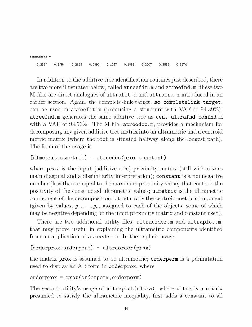
One of the difficulties in working with additive trees and displaying themgraphically is to find some sensible spot to site a root for the tree. Dependingon where the root is placed, a differing decomposition of D into an ultramet-ric and a centroid metric is implied. The ultrametric components inducedby the choice of root can differ widely with major substantive differencesin the branching patterns of the hierarchical clustering. The two M-filesdiscussed below, cent_ultrafnd_confit.m and cent_ultrafnd_confnd.m,both identify best-fitting additive trees to a given proximity matrix butwhere the terminal nodes of (an) ultrametric portion of the fitted matrixare then ordered according to a constraining order (conperm) that is eitherinput (in cent_ultrafnd_confit.m), or is identified as a good one to use(in cent_ultrafnd_confnd.m) and then given as an output vector. In bothcases, a centroid metric is first fit to the input proximity matrix; the resid-ual matrix is carried over to the order-constrained ultrametric constructionsroutines (ultrafnd_confit.m or ultrafnd_confnd.m), and thus, the root ischosen naturally for the ultrametric component. The whole process then iter-ates with a new centroid metric estimation, an order-constrained ultrametricre-estimation, and so on until convergence is achieved for the VAF values.

We illustrate below what occurs for our supreme_agree data and theimposition of the identity permutation (1:9) for the terminal nodes of theultrametric. The relevant outputs are the ultrametric component in targtwo

41

and the lengths for the centroid metric in lengthsone. To graph the additivetree, we first add .60 to the entries in targtwo to make them all positive andgraph this ultrametric as in Figure 4. Then, (1/2)(.60) = .30 is subtractedfrom each term in lengthsone; the branches attached to the terminal nodesof the ultrametric are then stretched or shrunk accordingly to produce Figure5. (These stretching/shrinking factors are as follows: St: (.07); Br: (−.05);Gi: (−.06); So: (−.09); Oc: (−.18); Ke: (−.14); Re: (−.10); Sc: (.06);Th: (.06).) We note that if cent_ultrafnd_confnd.m were invoked to finda good constraining order for the ultrametric component, the VAF could beincreased slightly (to 98.56% from 98.41% for Figure 5) using the conperm of[3 1 4 2 5 6 7 9 8]. No real substantive interpretative difference, however, isapparent from the structure given for a constraining identity permutation.

>> [find,vaf,outperm,targone,targtwo,lengthsone] = cent_ultrafnd_confit(supreme_agree,randperm(9),1:9)

find =

0 0.3800 0.3707 0.3793 0.6307 0.6643 0.7067 0.8634 0.8649

0.3800 0 0.2493 0.2579 0.5093 0.5429 0.5852 0.7420 0.7434

0.3707 0.2493 0 0.2428 0.4941 0.5278 0.5701 0.7269 0.7283

0.3793 0.2579 0.2428 0 0.4667 0.5003 0.5427 0.6994 0.7009

0.6307 0.5093 0.4941 0.4667 0 0.2745 0.3168 0.4736 0.4750

0.6643 0.5429 0.5278 0.5003 0.2745 0 0.2483 0.4051 0.4065

0.7067 0.5852 0.5701 0.5427 0.3168 0.2483 0 0.3293 0.3307

0.8634 0.7420 0.7269 0.6994 0.4736 0.4051 0.3293 0 0.2100

0.8649 0.7434 0.7283 0.7009 0.4750 0.4065 0.3307 0.2100 0

vaf =

0.9841

outperm =

1 2 3 4 5 6 7 8 9

targone =

0 0.6246 0.6094 0.5820 0.4977 0.5313 0.5737 0.7304 0.7319

0.6246 0 0.4880 0.4606 0.3763 0.4099 0.4522 0.6090 0.6104

0.6094 0.4880 0 0.4454 0.3611 0.3948 0.4371 0.5939 0.5953

0.5820 0.4606 0.4454 0 0.3337 0.3673 0.4097 0.5664 0.5679

0.4977 0.3763 0.3611 0.3337 0 0.2830 0.3253 0.4821 0.4836

0.5313 0.4099 0.3948 0.3673 0.2830 0 0.3590 0.5158 0.5172

0.5737 0.4522 0.4371 0.4097 0.3253 0.3590 0 0.5581 0.5595

0.7304 0.6090 0.5939 0.5664 0.4821 0.5158 0.5581 0 0.7163

0.7319 0.6104 0.5953 0.5679 0.4836 0.5172 0.5595 0.7163 0

targtwo =

0 -0.2446 -0.2387 -0.2027 0.1330 0.1330 0.1330 0.1330 0.1330

42

-0.2446 0 -0.2387 -0.2027 0.1330 0.1330 0.1330 0.1330 0.1330

-0.2387 -0.2387 0 -0.2027 0.1330 0.1330 0.1330 0.1330 0.1330

-0.2027 -0.2027 -0.2027 0 0.1330 0.1330 0.1330 0.1330 0.1330

0.1330 0.1330 0.1330 0.1330 0 -0.0085 -0.0085 -0.0085 -0.0085

0.1330 0.1330 0.1330 0.1330 -0.0085 0 -0.1107 -0.1107 -0.1107

0.1330 0.1330 0.1330 0.1330 -0.0085 -0.1107 0 -0.2288 -0.2288

0.1330 0.1330 0.1330 0.1330 -0.0085 -0.1107 -0.2288 0 -0.5063

0.1330 0.1330 0.1330 0.1330 -0.0085 -0.1107 -0.2288 -0.5063 0

lengthsone =

0.3730 0.2516 0.2364 0.2090 0.1247 0.1583 0.2007 0.3574 0.3589

>> [find,vaf,outperm,targone,targtwo,lengthsone] = cent_ultrafnd_confnd(supreme_agree,randperm(9))

find =

0 0.3400 0.2271 0.2794 0.4974 0.5310 0.5734 0.7316 0.7301

0.3400 0 0.3629 0.4151 0.6331 0.6667 0.7091 0.8673 0.8659

0.2271 0.3629 0 0.2556 0.4736 0.5072 0.5495 0.7078 0.7063

0.2794 0.4151 0.2556 0 0.4967 0.5303 0.5727 0.7309 0.7294

0.4974 0.6331 0.4736 0.4967 0 0.2745 0.3168 0.4750 0.4736

0.5310 0.6667 0.5072 0.5303 0.2745 0 0.2483 0.4065 0.4051

0.5734 0.7091 0.5495 0.5727 0.3168 0.2483 0 0.3307 0.3293

0.7316 0.8673 0.7078 0.7309 0.4750 0.4065 0.3307 0 0.2100

0.7301 0.8659 0.7063 0.7294 0.4736 0.4051 0.3293 0.2100 0

vaf =

0.9856

outperm =

3 1 4 2 5 6 7 9 8

targone =

0 0.6151 0.4556 0.4787 0.3644 0.3980 0.4404 0.5986 0.5971

0.6151 0 0.5913 0.6144 0.5001 0.5337 0.5761 0.7343 0.7329

0.4556 0.5913 0 0.4549 0.3406 0.3742 0.4165 0.5748 0.5733

0.4787 0.6144 0.4549 0 0.3637 0.3973 0.4397 0.5979 0.5964

0.3644 0.5001 0.3406 0.3637 0 0.2830 0.3253 0.4836 0.4821

0.3980 0.5337 0.3742 0.3973 0.2830 0 0.3590 0.5172 0.5158

0.4404 0.5761 0.4165 0.4397 0.3253 0.3590 0 0.5595 0.5581

0.5986 0.7343 0.5748 0.5979 0.4836 0.5172 0.5595 0 0.7163

0.5971 0.7329 0.5733 0.5964 0.4821 0.5158 0.5581 0.7163 0

targtwo =

0 -0.2751 -0.2284 -0.1993 0.1330 0.1330 0.1330 0.1330 0.1330

-0.2751 0 -0.2284 -0.1993 0.1330 0.1330 0.1330 0.1330 0.1330

-0.2284 -0.2284 0 -0.1993 0.1330 0.1330 0.1330 0.1330 0.1330

-0.1993 -0.1993 -0.1993 0 0.1330 0.1330 0.1330 0.1330 0.1330

0.1330 0.1330 0.1330 0.1330 0 -0.0085 -0.0085 -0.0085 -0.0085

0.1330 0.1330 0.1330 0.1330 -0.0085 0 -0.1107 -0.1107 -0.1107

0.1330 0.1330 0.1330 0.1330 -0.0085 -0.1107 0 -0.2288 -0.2288

0.1330 0.1330 0.1330 0.1330 -0.0085 -0.1107 -0.2288 0 -0.5063

0.1330 0.1330 0.1330 0.1330 -0.0085 -0.1107 -0.2288 -0.5063 0

43

lengthsone =

0.2397 0.3754 0.2159 0.2390 0.1247 0.1583 0.2007 0.3589 0.3574

In addition to the additive tree identification routines just described, thereare two more illustrated below, called atreefit.m and atreefnd.m; these twoM-files are direct analogues of ultrafit.m and ultrafnd.m introduced in anearlier section. Again, the complete-link target, sc_completelink_target,can be used in atreefit.m (producing a structure with VAF of 94.89%);atreefnd.m generates the same additive tree as cent_ultrafnd_confnd.m

with a VAF of 98.56%. The M-file, atreedec.m, provides a mechanism fordecomposing any given additive tree matrix into an ultrametric and a centroidmetric matrix (where the root is situated halfway along the longest path).The form of the usage is

[ulmetric,ctmetric] = atreedec(prox,constant)

where prox is the input (additive tree) proximity matrix (still with a zeromain diagonal and a dissimilarity interpretation); constant is a nonnegativenumber (less than or equal to the maximum proximity value) that controls thepositivity of the constructed ultrametric values; ulmetric is the ultrametriccomponent of the decomposition; ctmetric is the centroid metric component(given by values, g1, . . . , gn, assigned to each of the objects, some of whichmay be negative depending on the input proximity matrix and constant used).

There are two additional utility files, ultraorder.m and ultraplot.m,that may prove useful in explaining the ultrametric components identifiedfrom an application of atreedec.m. In the explicit usage

[orderprox,orderperm] = ultraorder(prox)

the matrix prox is assumed to be ultrametric; orderperm is a permutationused to display an AR form in orderprox, where

orderprox = prox(orderperm,orderperm)

The second utility’s usage of ultraplot(ultra), where ultra is a matrixpresumed to satisfy the ultrametric inequality, first adds a constant to all

44

Figure 4: A Dendrogram (Tree) Representation for the Ordered-Constrained UltrametricComponent of the Additive Tree Represented in Figure 5


i i i i i i i i i

yy

~

y

y

y

y-.09

-.36 -.37-.40

-.49

-.59

-.73

45

Figure 5: An Graph-Theoretic Representation for the Ordered-Constrained Additive TreeDescribed in the Text (Having VAF of 98.41%)

St

BrGi

So

Oc

Ke

Re

Sc Th

i

ii

i

i

i

i

i i

yy

~

y

y

y

y

-.00

-.10

-.20

-.30

-.40

-.50

46

values in ultra to make the entries positive; the MATLAB Statistics Tool-box routine, dendrogram.m, is then invoked to plot the resulting ultrametricmatrix.


>> load sc_completelink_target.dat

>> [fit,vaf] = atreefit(supreme_agree,sc_completelink_target)

fit =

0 0.3972 0.3850 0.3678 0.6748 0.6670 0.6756 0.8456 0.8470

0.3972 0 0.2635 0.2464 0.5533 0.5456 0.5542 0.7242 0.7256

0.3850 0.2635 0 0.2200 0.5411 0.5333 0.5419 0.7119 0.7133

0.3678 0.2464 0.2200 0 0.5239 0.5162 0.5247 0.6947 0.6962

0.6748 0.5533 0.5411 0.5239 0 0.2449 0.2535 0.4235 0.4249

0.6670 0.5456 0.5333 0.5162 0.2449 0 0.2300 0.4158 0.4172

0.6756 0.5542 0.5419 0.5247 0.2535 0.2300 0 0.4243 0.4258

0.8456 0.7242 0.7119 0.6947 0.4235 0.4158 0.4243 0 0.2100

0.8470 0.7256 0.7133 0.6962 0.4249 0.4172 0.4258 0.2100 0

vaf =

0.9489

>> [find,vaf] = atreefnd(supreme_agree,randperm(9))

find =

0 0.4151 0.3400 0.3629 0.6329 0.6668 0.7091 0.8659 0.8673

0.4151 0 0.2794 0.2556 0.4965 0.5304 0.5727 0.7295 0.7309

0.3400 0.2794 0 0.2271 0.4972 0.5311 0.5734 0.7302 0.7316

0.3629 0.2556 0.2271 0 0.4734 0.5073 0.5496 0.7064 0.7078

0.6329 0.4965 0.4972 0.4734 0 0.2745 0.3168 0.4736 0.4750

0.6668 0.5304 0.5311 0.5073 0.2745 0 0.2483 0.4051 0.4065

0.7091 0.5727 0.5734 0.5496 0.3168 0.2483 0 0.3293 0.3307

0.8659 0.7295 0.7302 0.7064 0.4736 0.4051 0.3293 0 0.2100

0.8673 0.7309 0.7316 0.7078 0.4750 0.4065 0.3307 0.2100 0

vaf =

0.9856

>> [ulmetric,ctmetric] = atreedec(find,1.0)

ulmetric =

0 0.8168 0.7410 0.7877 1.1327 1.1327 1.1327 1.1327 1.1327

0.8168 0 0.8168 0.8168 1.1327 1.1327 1.1327 1.1327 1.1327

0.7410 0.8168 0 0.7877 1.1327 1.1327 1.1327 1.1327 1.1327

0.7877 0.8168 0.7877 0 1.1327 1.1327 1.1327 1.1327 1.1327

1.1327 1.1327 1.1327 1.1327 0 0.9748 0.9748 0.9748 0.9748

1.1327 1.1327 1.1327 1.1327 0.9748 0 0.8724 0.8724 0.8724

1.1327 1.1327 1.1327 1.1327 0.9748 0.8724 0 0.7543 0.7543

1.1327 1.1327 1.1327 1.1327 0.9748 0.8724 0.7543 0 0.4768

1.1327 1.1327 1.1327 1.1327 0.9748 0.8724 0.7543 0.4768 0

ctmetric =

47

-0.1327

-0.2691

-0.2684

-0.2922

-0.3671

-0.3332

-0.2909

-0.1341

-0.1327

>> [orderprox,orderperm] = ultraorder(ulmetric)

orderprox =

0 0.7877 0.7877 0.8168 1.1327 1.1327 1.1327 1.1327 1.1327

0.7877 0 0.7410 0.8168 1.1327 1.1327 1.1327 1.1327 1.1327

0.7877 0.7410 0 0.8168 1.1327 1.1327 1.1327 1.1327 1.1327

0.8168 0.8168 0.8168 0 1.1327 1.1327 1.1327 1.1327 1.1327

1.1327 1.1327 1.1327 1.1327 0 0.7543 0.7543 0.8724 0.9748

1.1327 1.1327 1.1327 1.1327 0.7543 0 0.4768 0.8724 0.9748

1.1327 1.1327 1.1327 1.1327 0.7543 0.4768 0 0.8724 0.9748

1.1327 1.1327 1.1327 1.1327 0.8724 0.8724 0.8724 0 0.9748

1.1327 1.1327 1.1327 1.1327 0.9748 0.9748 0.9748 0.9748 0

orderperm =

4 3 1 2 7 8 9 6 5

7 Some Bibliographic Comments

There are a number of book-length presentations of cluster analysis methodsavailable (encompassing differing collections of subtopics within the field).We list several of the better ones to consult in the reference section to fol-low, and note these here in chronological order: Anderberg (1973); Hartigan(1975); Spath (1980); Barthelemy and Guenoche (1991); Mirkin (1996); Ara-bie, Hubert, and DeSoete (1996); Everitt and Rabe-Hesketh (1997); Gordon(1999). The items that would be closest to the approaches taken here withMATLAB and the emphasis on least-squares, would be the monograph byHubert, Arabie, and Meulman (2006), and the review articles by Hubert,Kohn, and Steinley (in press); and Steinley and Hubert (2008).

48

References

[1] Anderberg, M. (1973). Cluster analysis for applications. New York: Aca-demic Press.

[2] Arabie, P., Hubert, L., & DeSoete, G. (Eds.) (1996). Clustering andclassification. River Edge, NJ: World Scientific.

[3] Barthelemy, J.-P., & Guenoche, A. (1991). Trees and proximity repre-sentations. Chichester: Wiley.

[4] Brossier, G. (1987). Etude des matrices de proximite rectangulaires envue de la classification [A study of rectangular proximity matrices fromthe point of view of classification]. Revue de Statistiques Appliquees,35(4), 43–68.

[5] Everitt, B. S., & Rabe-Hesketh, S. (1997). The analysis of proximitydata. New York: Wiley.

[6] Furnas, G. W. (1980). Objects and their features: The metric repre-sentation of two class data. Unpublished doctoral dissertation, StanfordUniversity.

[7] Gordon, A. D. (1999). Classification. London: Chapman & Hall/CRC.

[8] Hartigan, J. (1975). Clustering algorithms. New York: Wiley.

[9] Hubert, L., Arabie, P., & Meulman, J. (2006). The structural repre-sentation of proximity matrices with MATLAB. ASA-SIAM Series onStatistics and Applied Probability. Philadelphia: SIAM.

[10] Hubert, L., Kohn, H.-F., & Steinley, D. (in press). Order-constrainedproximity matrix representations: Ultrametric generalizations and con-structions with MATLAB. To appear in: Methodological developmentsof statistics in the social sciences. New York: Wiley.

[11] Mirkin, B. (1996). Mathematical classification and clustering. Dordrecht:Kluwer.

49

[12] Spath, H. (1980). Cluster analysis algorithms. Chichester, U.K.: EllisHorwood.

[13] Steinley, D., & Hubert, L. (2008). Order constrained solutions in K-means clustering: Even better than being globally optimal. Psychome-trika, 73, xxx–xxx.

[14] Wollan, P. C., & Dykstra, R. L. (1987). Minimizing linear inequalityconstrained Mahalanobis distances. Applied Statistics, 36, 234–240.

50

8 Ultrametric Extensions by Fitting Partitions Con-

taining Contiguous Subsets

The M-file, partitionfit.m, is a very general routine giving a least-squaresapproximation to a proximity matrix based on a given collection of parti-tions. Thus, no matter how the set of candidate partitions might be chosen,a least-squares fitted matrix to the given proximity matrix is achieved. Forexample, if we simply use the nested partitions constructed from an ultramet-ric, the ultrametric would be retrieved when the latter is used as the inputproximity matrix. In this section, we show how partitionfit.m can alsobe used to select partitions from a predefined set (this selection is done bythose partitions assigned strictly positive weights) that might serve to recon-struct the proximity matrix well. The M-file, consec_subsetfit.m, defines(n(n−1)/2)−1 candidate partitions each characterized by a single contiguouscluster of objects, with all objects before and after this contiguous set formingindividual clusters of the partition (the minus 1 appears in the count due tothe (conjoint) partition defined by a single contiguous set being excluded).The M-file, consec_subsetfit_alter.m, varies the specific definition of thepartitions by including all objects before and all objects after the contiguousset (when nonempty) as separate individual clusters of the partitions.

As can be seen from the verbatim output provided below, the nonnegativeweighted partitions from consec_subsetfit.m, producing a fitted matrixwith VAF of 92.61%, are as follows:

Partition Partition Increment

{{St,Br,Gi,So},{Oc},{Ke},{Re},{Sc},{Th}} .1939{{St,Br,Gi,So,Oc},{Ke},{Re},{Sc},{Th}} .0300{{St,Br,Gi,So,Oc,Ke},{Re},{Sc},{Th}} .0389{{St,Br,Gi,So,Oc,Ke,Re},{Sc},{Th}} .1315{{St},{Br,Gi,So,Oc,Ke,Re,Sc,Th}} .1152{{St},{Br},{Gi,So,Oc,Ke,Re,Sc,Th}} .0052{{St},{Br},{Gi},{So,Oc,Ke,Re,Sc,Th}} .0153{{St},{Br},{Gi},{So},{Oc,Ke,Re,Sc,Th}} .2220{{St},{Br},{Gi},{So},{Oc},{Ke,Re,Sc,Th}} .0633{{St},{Br},{Gi},{So},{Oc},{Ke},{Re,Sc,Th}} .0030

Similarly, we have a very high VAF of 98.12% based on the more numerouspartitions generated from consec_subsetfit_alter.m:

51


{{St,Br},{Gi,So,Oc,Ke,Re,Sc,Th}} .0021{{St,Br,Gi},{So,Oc,Ke,Re,Sc,Th}} .0001{{St,Br,Gi,So},{Oc,Ke,Re,Sc,Th}} .0001{{St,Br,Gi,So,Oc,Ke},{Re,Sc,Th}} .0100{{St,Br,Gi,So,Oc,Ke,Re},{Sc,Th}} .1218{{St},{Br,Gi},{So,Oc,Ke,Re,Sc,Th}} .0034{{St},{Br,Gi,So,Oc},{Ke,Re,Sc,Th}} .0056{{St},{Br,Gi,So,Oc,Ke,Re},{Sc,Th}} .0113{{St},{Br,Gi,So,Oc,Ke,Re,Sc},{Th}} .0038{{St},{Br,Gi,So,Oc,Ke,Re,Sc,Th}} .1170{{St,Br},{Gi,So},{Oc,Ke,Re,Sc,Th}} .0165{{St,Br},{Gi,So,Oc,Ke,Re,Sc,Th}} .0095{{St,Br,Gi},{So,Oc},{Ke,Re,Sc,Th}} .0197{{St,Br,Gi},{So,Oc,Ke,Re,Sc,Th}} .0115{{St,Br,Gi,So},{Oc,Ke,Re,Sc,Th}} .2294{{St,Br,Gi,So,Oc},{Ke,Re,Sc,Th}} .0353{{St,Br,Gi,So,Oc,Ke},{Re,Sc,Th}} .0400{{St,Br,Gi,So,Oc,Ke,Re},{Sc,Th}} .0132

{{St},{Br},{Gi},{So},{Oc},{Ke},{Re},{Sc},{Th}} .2050


>> [fitted,vaf,weights,end_condition,member] = consec_subsetfit(supreme_agree);

>> fitted

fitted =

0 0.4239 0.4239 0.4239 0.6178 0.6478 0.6866 0.8181 0.8181

0.4239 0 0.3087 0.3087 0.5026 0.5326 0.5715 0.7029 0.7029

0.4239 0.3087 0 0.3035 0.4974 0.5274 0.5663 0.6977 0.6977

0.4239 0.3087 0.3035 0 0.4821 0.5121 0.5510 0.6824 0.6824

0.6178 0.5026 0.4974 0.4821 0 0.2901 0.3290 0.4604 0.4604

0.6478 0.5326 0.5274 0.5121 0.2901 0 0.2657 0.3972 0.3972

0.6866 0.5715 0.5663 0.5510 0.3290 0.2657 0 0.3942 0.3942

0.8181 0.7029 0.6977 0.6824 0.4604 0.3972 0.3942 0 0.3942

0.8181 0.7029 0.6977 0.6824 0.4604 0.3972 0.3942 0.3942 0

>> vaf

vaf =

0.9261

>> weights

weights =

0

0

0.1939

0.0300

0.0389

0.1315

0

0

0

0

0

0

0

0.1152

0

0

0

52

0

0

0.0052

0

0

0

0

0.0153

0

0

0

0.2220

0

0

0.0633

0

0.0030

0

0

>> end_condition

end_condition =

0

>> member

member =

1 1 3 4 5 6 7 8 9

1 1 1 4 5 6 7 8 9

1 1 1 1 5 6 7 8 9

1 1 1 1 1 6 7 8 9

1 1 1 1 1 1 7 8 9

1 1 1 1 1 1 1 8 9

1 1 1 1 1 1 1 1 9

1 2 2 4 5 6 7 8 9

1 2 2 2 5 6 7 8 9

1 2 2 2 2 6 7 8 9

1 2 2 2 2 2 7 8 9

1 2 2 2 2 2 2 8 9

1 2 2 2 2 2 2 2 9

1 2 2 2 2 2 2 2 2

1 2 3 3 5 6 7 8 9

1 2 3 3 3 6 7 8 9

1 2 3 3 3 3 7 8 9

1 2 3 3 3 3 3 8 9

1 2 3 3 3 3 3 3 9

1 2 3 3 3 3 3 3 3

1 2 3 4 4 6 7 8 9

1 2 3 4 4 4 7 8 9

1 2 3 4 4 4 4 8 9

1 2 3 4 4 4 4 4 9

1 2 3 4 4 4 4 4 4

1 2 3 4 5 5 7 8 9

1 2 3 4 5 5 5 8 9

1 2 3 4 5 5 5 5 9

1 2 3 4 5 5 5 5 5

1 2 3 4 5 6 6 8 9

1 2 3 4 5 6 6 6 9

1 2 3 4 5 6 6 6 6

1 2 3 4 5 6 7 7 9

1 2 3 4 5 6 7 7 7

53

1 2 3 4 5 6 7 8 8

1 2 3 4 5 6 7 8 9

>> [fitted,vaf,weights,end_condition,member] = consec_subsetfit_alter(supreme_agree)

fitted =

0 0.3460 0.3740 0.4053 0.6347 0.6700 0.7200 0.8550 0.8550

0.3460 0 0.2330 0.2677 0.4971 0.5380 0.5880 0.7342 0.7380

0.3740 0.2330 0 0.2396 0.4855 0.5264 0.5764 0.7227 0.7264

0.4053 0.2677 0.2396 0 0.4509 0.5114 0.5614 0.7076 0.7114

0.6347 0.4971 0.4855 0.4509 0 0.2655 0.3155 0.4617 0.4655

0.6700 0.5380 0.5264 0.5114 0.2655 0 0.2550 0.4012 0.4050

0.7200 0.5880 0.5764 0.5614 0.3155 0.2550 0 0.3512 0.3550

0.8550 0.7342 0.7227 0.7076 0.4617 0.4012 0.3512 0 0.2087

0.8550 0.7380 0.7264 0.7114 0.4655 0.4050 0.3550 0.2087 0

vaf =

0.9812

weights =

0.0021

0.0001

0.0001

0

0.0100

0.1218

0

0.0034

0

0.0056

0

0.0113

0.0038

0.1170

0.0165

0

0

0

0

0.0095

0.0197

0

0

0

0.0115

0

0

0

0.2294

0

0

0.0353

0

0.0400

0.0132

0.2050

54

end_condition =

0

member =

1 1 9 9 9 9 9 9 9

1 1 1 9 9 9 9 9 9

1 1 1 1 9 9 9 9 9

1 1 1 1 1 9 9 9 9

1 1 1 1 1 1 9 9 9

1 1 1 1 1 1 1 9 9

1 1 1 1 1 1 1 1 9

1 2 2 9 9 9 9 9 9

1 2 2 2 9 9 9 9 9

1 2 2 2 2 9 9 9 9

1 2 2 2 2 2 9 9 9

1 2 2 2 2 2 2 9 9

1 2 2 2 2 2 2 2 9

1 2 2 2 2 2 2 2 2

1 1 3 3 9 9 9 9 9

1 1 3 3 3 9 9 9 9

1 1 3 3 3 3 9 9 9

1 1 3 3 3 3 3 9 9

1 1 3 3 3 3 3 3 9

1 1 3 3 3 3 3 3 3

1 1 1 4 4 9 9 9 9

1 1 1 4 4 4 9 9 9

1 1 1 4 4 4 4 9 9

1 1 1 4 4 4 4 4 9

1 1 1 4 4 4 4 4 4

1 1 1 1 5 5 9 9 9

1 1 1 1 5 5 5 9 9

1 1 1 1 5 5 5 5 9

1 1 1 1 5 5 5 5 5

1 1 1 1 1 6 6 9 9

1 1 1 1 1 6 6 6 9

1 1 1 1 1 6 6 6 6

1 1 1 1 1 1 7 7 9

1 1 1 1 1 1 7 7 7

1 1 1 1 1 1 1 8 8

1 2 3 4 5 6 7 8 9

To see how well one might do by choosing only eight partitions (i.e., thesame number needed to define the order-constrained best-fitting ultramet-ric), the single (disjoint) partition defined by nine separate classes is cho-sen in both instances, plus the seven partitions having the highest assignedpositive weights. For those picked from the partition pool identified byconsec_subsetfit.m, the VAF drops slightly from 92.61% to 92.51% basedon the partitions:

55


{{St,Br,Gi,So},{Oc},{Ke},{Re},{Sc},{Th}} .1923{{St,Br,Gi,So,Oc},{Ke},{Re},{Sc},{Th}} .0301{{St,Br,Gi,So,Oc,Ke},{Re},{Sc},{Th}} .0396{{St,Br,Gi,So,Oc,Ke,Re},{Sc},{Th}} .1316{{St},{Br,Gi,So,Oc,Ke,Re,Sc,Th}} .1224

{{St},{Br},{Gi},{So},{Oc,Ke,Re,Sc,Th}} .2250{{St},{Br},{Gi},{So},{Oc},{Ke,Re,Sc,Th}} .0671


For those selected from the set generated by consec_subsetfit_alter.m,the VAF again drops slightly from 98.12% to 97.97%. But in some absolutesense given the size of the VAF, the eight partitions listed below seem to beabout all that can be extracted from this particular justice data set.


{{St,Br,Gi,So,Oc,Ke,Re},{Sc,Th}} .1466{{St},{Br,Gi,So,Oc,Ke,Re,Sc,Th}} .1399{{St,Br},{Gi,So},{Oc,Ke,Re,Sc,Th}} .0287{{St,Br,Gi},{So,Oc},{Ke,Re,Sc,Th}} .0326{{St,Br,Gi,So},{Oc,Ke,Re,Sc,Th}} .2269{{St,Br,Gi,So,Oc},{Ke,Re,Sc,Th}} .0316{{St,Br,Gi,So,Oc,Ke},{Re,Sc,Th}} .0500


The three highest weighted partitions have very clear interpretations:

{Sc,Th} versus the rest; {St} versus the rest; {St,Br,Gi,So} as the left versus{Oc,Ke,Re,Sc,Th} as the right. The few remaining partitions revolve aroundseveral other less salient (adjacent) object pairings that are also very inter-pretable in relation to the object ordering from liberal to conservative. Wegive a graphical representation for this latter culled collection of partitions inFigure 6. Again, the partition increments are not included in a fitted valuewhenever a continuous horizontal line encompasses the relevant objects in adefining cluster of the partition.

>> member = [1 1 1 1 5 6 7 8 9;1 1 1 1 1 6 7 8 9;1 1 1 1 1 1 7 8 9;1 1 1 1 1 1 1 8 9;

1 2 2 2 2 2 2 2 2;1 2 3 4 5 5 5 5 5;1 2 3 4 5 6 6 6 6;1 2 3 4 5 6 7

8 9]

member =

1 1 1 1 5 6 7 8 9

1 1 1 1 1 6 7 8 9

1 1 1 1 1 1 7 8 9

1 1 1 1 1 1 1 8 9

1 2 2 2 2 2 2 2 2

1 2 3 4 5 5 5 5 5

1 2 3 4 5 6 6 6 6

56

Figure 6: A Representation for the Fitted Values of the (Generalized) Structure Describedin the Text (Having VAF of 97.97%)


i i i i i i i i i-.21

-.23

-.15

-.14

-.05-.03-.03-.03

57

1 2 3 4 5 6 7 8 9


fitted =

0 0.4245 0.4245 0.4245 0.6168 0.6469 0.6865 0.8181 0.8181

0.4245 0 0.3021 0.3021 0.4944 0.5245 0.5641 0.6957 0.6957

0.4245 0.3021 0 0.3021 0.4944 0.5245 0.5641 0.6957 0.6957

0.4245 0.3021 0.3021 0 0.4944 0.5245 0.5641 0.6957 0.6957

0.6168 0.4944 0.4944 0.4944 0 0.2895 0.3291 0.4607 0.4607

0.6469 0.5245 0.5245 0.5245 0.2895 0 0.2620 0.3936 0.3936

0.6865 0.5641 0.5641 0.5641 0.3291 0.2620 0 0.3936 0.3936

0.8181 0.6957 0.6957 0.6957 0.4607 0.3936 0.3936 0 0.3936

0.8181 0.6957 0.6957 0.6957 0.4607 0.3936 0.3936 0.3936 0

vaf =

0.9251

weights =

0.1923

0.0301

0.0396

0.1316

0.1224

0.2350

0.0671

0

end_condition =

0

>> member = [1 1 1 1 1 1 1 9 9;1 2 2 2 2 2 2 2 2;1 1 3 3 9 9 9 9 9;1 1 1 4 4 9 9 9 9;

1 1 1 1 5 5 5 5 5;1 1 1 1 1 6 6 6 6;1 1 1 1 1 1 7 7 7;1 2 3 4 5 6 7

8 9]

member =

1 1 1 1 1 1 1 9 9

1 2 2 2 2 2 2 2 2

1 1 3 3 9 9 9 9 9

1 1 1 4 4 9 9 9 9

1 1 1 1 5 5 5 5 5

1 1 1 1 1 6 6 6 6

1 1 1 1 1 1 7 7 7

1 2 3 4 5 6 7 8 9


fitted =

0 0.3450 0.3736 0.4062 0.6331 0.6647 0.7147 0.8613 0.8613

0.3450 0 0.2337 0.2664 0.4933 0.5248 0.5748 0.7215 0.7215

0.3736 0.2337 0 0.2377 0.4933 0.5248 0.5748 0.7215 0.7215

0.4062 0.2664 0.2377 0 0.4606 0.5248 0.5748 0.7215 0.7215

0.6331 0.4933 0.4933 0.4606 0 0.2693 0.3193 0.4659 0.4659

0.6647 0.5248 0.5248 0.5248 0.2693 0 0.2551 0.4017 0.4017

0.7147 0.5748 0.5748 0.5748 0.3193 0.2551 0 0.3517 0.3517

58

0.8613 0.7215 0.7215 0.7215 0.4659 0.4017 0.3517 0 0.2051

0.8613 0.7215 0.7215 0.7215 0.4659 0.4017 0.3517 0.2051 0

vaf =

0.9797

weights =

0.1466

0.1399

0.0287

0.0326

0.2269

0.0316

0.0500

0.2051

end_condition =

0

9 Ultrametrics and Additive Trees for Two-Mode

(Rectangular) Proximity Data

The proximity data considered thus far for obtaining some type of structure,such as an ultrametric or an additive tree, have been assumed to be onone intact set of objects, S = {O1, . . . , On}, and complete in the sense thatproximity values are present between all object pairs. Suppose now thatthe available proximity data are two-mode, and between two distinct objectsets, SA = {O1A, . . . , OnaA} and SB = {O1B, . . . , OnbB}, containing na andnb objects, respectively, given by an na × nb proximity matrix Q = {qrs}.Again, we assume that the entries in Q are keyed as dissimilarities, anda joint structural representation is desired for the combined set SA ∪ SB.We might caution at the outset of the need to have legitimate proximitiesto make the analyses to follow very worthwhile or interpretable. There aremany numerical elicitation schemes where subjects (e.g., raters) are askedto respond to some set of objects (e.g., items). If the elicitation is for, say,preference, then proximity may be a good interpretation for the numericalvalues. If, on the other hand, the numerical value is merely a rating given onsome more-or-less objective criterion where only errors of observation induce

59

the variability from rater to rater, then probably not.

Conditions have been proposed in the literature for when the entries in amatrix fitted to Q characterize an ultrametric or an additive tree represen-tation. In particular, suppose an na × nb matrix, F = {frs}, is fitted to Qthrough least squares subject to the constraints that follow:

Ultrametric (Furnas, 1980):

for all distinct object quadruples, OrA, OsA, OrB, OsB, where OrA, OsA ∈ SA

and OrB, OsB, ∈ SB, and considering the entries in F corresponding to thepairs, (OrA, OrB), (OrA, OsB), (OsA OrB), and (OsA, OsB), say frArB

, frAsB,

fsArB, fsAsB

, respectively, the largest two must be equal.

Additive trees (Brossier, 1987):

for all distinct object sextuples, OrA, OsA, OtA, OrB, OsB, OtB, where OrA,OsA, OtA ∈ SA and OrB, OsB, OtB, ∈ SB, and considering the entries in Fcorresponding to the pairs (OrA, OrB), (OrA, OsB), (OrA, OtB), (OsA, OrB),(OsA, OsB), (OsA, OtB), (OtA, OrB), (OtA, OsB), and (OtA, OtB), say frArB

,frAsB

, frAtB , fsArB, fsAsB

, fsAtB , ftArB, ftAsB

, ftAtB , respectively, the largest twoof the following sums must be equal:

frArB+ fsAsB

+ ftAtB ;frArB

+ fsAtB + ftAsB;

frAsB+ fsArB

+ ftAtB ;frAsB

+ fsAtB + ftArB;

frAtB + fsArB+ ftAsB

;frAtB + fsAsB

+ ftArB.

9.1 Two-Mode Ultrametrics

To illustrate the fitting of a given two-mode ultrametric, a two-mode targetis generated by extracting a 5× 4 portion from the 9× 9 ultrametric targetmatrix, sc_completelink_target, used earlier. This file has contents asfollows (sc_completelink_target5x4.dat):

0.3800 0.3800 0.8600 0.8600

0.2900 0.2200 0.8600 0.8600

0.8600 0.8600 0.3300 0.4600

0.8600 0.8600 0.2300 0.4600

0.8600 0.8600 0.4600 0.2100

60

The five rows correspond to the judges, St, Gi, Oc, Re, Th; the four columnsto Br, So, Ke, Sc. As the two-mode 5 × 4 proximity matrix, the appro-priate portion of the supreme_agree proximity matrix will be used in thefitting process; the corresponding file is called supreme_agree5x4.dat, withcontents:

0.3000 0.3700 0.6400 0.8600

0.2800 0.2200 0.5100 0.7200

0.4500 0.4500 0.3300 0.4600

0.5700 0.5600 0.2300 0.3400

0.7600 0.7100 0.4100 0.2100

Because of the way the joint set of row and columns objects is numbered, thefive rows are labeled from 1 to 5 and the four columns from 6 to 9. Thus, thecorrespondence between the justices and the numbers obviously differs fromearlier applications:

1:St; 2:Gi; 3:Oc; 4:Re; 5:Th; 6:Br; 7:So; 8:Ke; 9:Sc

The M-file, ultrafittm.m, fits a given ultrametric to a two-mode proxim-ity matrix, and has usage

[fit,vaf] = ultrafittm(proxtm,targ)

where proxtm is the two-mode (rectangular) input proximity matrix (with adissimilarity interpretation); targ is an ultrametric matrix of the same size asproxtm; fit is the least-squares optimal matrix (with variance-accounted-forof vaf) to proxtm satisfying the two-mode ultrametric constraints implicit intarg. An example follows using sc_completelink_target5x4 for targ andsupreme_agree5x4 as proxtm:

>> load supreme_agree5x4.dat

>> load sc_completelink_target5x4.dat

>> supreme_agree5x4

supreme_agree5x4 =

0.3000 0.3700 0.6400 0.8600

0.2800 0.2200 0.5100 0.7200

0.4500 0.4500 0.3300 0.4600

0.5700 0.5600 0.2300 0.3400

0.7600 0.7100 0.4100 0.2100

>> sc_completelink_target5x4

sc_completelink_target5x4 =

61

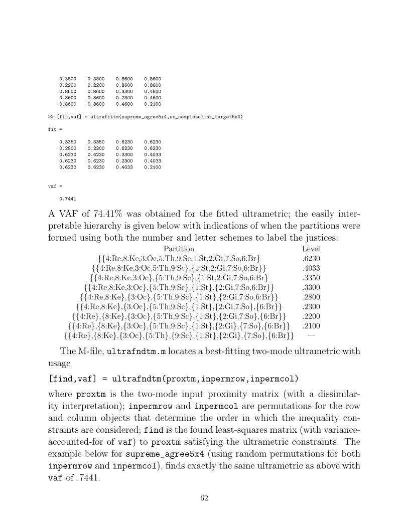
0.3800 0.3800 0.8600 0.8600

0.2900 0.2200 0.8600 0.8600

0.8600 0.8600 0.3300 0.4600

0.8600 0.8600 0.2300 0.4600

0.8600 0.8600 0.4600 0.2100

>> [fit,vaf] = ultrafittm(supreme_agree5x4,sc_completelink_target5x4)

fit =

0.3350 0.3350 0.6230 0.6230

0.2800 0.2200 0.6230 0.6230

0.6230 0.6230 0.3300 0.4033

0.6230 0.6230 0.2300 0.4033

0.6230 0.6230 0.4033 0.2100

vaf =

0.7441

A VAF of 74.41% was obtained for the fitted ultrametric; the easily inter-pretable hierarchy is given below with indications of when the partitions wereformed using both the number and letter schemes to label the justices:

Partition Level{{4:Re,8:Ke,3:Oc,5:Th,9:Sc,1:St,2:Gi,7:So,6:Br} .6230

{{4:Re,8:Ke,3:Oc,5:Th,9:Sc},{1:St,2:Gi,7:So,6:Br}} .4033{{4:Re,8:Ke,3:Oc},{5:Th,9:Sc},{1:St,2:Gi,7:So,6:Br} .3350

{{4:Re,8:Ke,3:Oc},{5:Th,9:Sc},{1:St},{2:Gi,7:So,6:Br}} .3300{{4:Re,8:Ke},{3:Oc},{5:Th,9:Sc},{1:St},{2:Gi,7:So,6:Br}} .2800{{4:Re,8:Ke},{3:Oc},{5:Th,9:Sc},{1:St},{2:Gi,7:So},{6:Br}} .2300{{4:Re},{8:Ke},{3:Oc},{5:Th,9:Sc},{1:St},{2:Gi,7:So},{6:Br}} .2200{{4:Re},{8:Ke},{3:Oc},{5:Th,9:Sc},{1:St},{2:Gi},{7:So},{6:Br}} .2100{{4:Re},{8:Ke},{3:Oc},{5:Th},{9:Sc},{1:St},{2:Gi},{7:So},{6:Br}} —

The M-file, ultrafndtm.m locates a best-fitting two-mode ultrametric withusage

[find,vaf] = ultrafndtm(proxtm,inpermrow,inpermcol)

where proxtm is the two-mode input proximity matrix (with a dissimilar-ity interpretation); inpermrow and inpermcol are permutations for the rowand column objects that determine the order in which the inequality con-straints are considered; find is the found least-squares matrix (with variance-accounted-for of vaf) to proxtm satisfying the ultrametric constraints. Theexample below for supreme_agree5x4 (using random permutations for bothinpermrow and inpermcol), finds exactly the same ultrametric as above withvaf of .7441.

62

>> [find,vaf] = ultrafndtm(supreme_agree5x4,randperm(5),randperm(4))

find =

0.3350 0.3350 0.6230 0.6230

0.2800 0.2200 0.6230 0.6230

0.6230 0.6230 0.3300 0.4033

0.6230 0.6230 0.2300 0.4033

0.6230 0.6230 0.4033 0.2100

vaf =

0.7441

9.2 Two-Mode Additive Trees

The identification of a best-fitting two-mode additive tree will be done some-what differently than for a two-mode ultrametric representation, largely be-cause of future storage considerations when huge matrices might be consid-ered. Specifically, a (two-mode) centroid metric and a (two-mode) ultrametricmatrix will be identified so that their sum is a good-fitting two-mode addi-tive tree. Because a centroid metric can be obtained in closed-form, we firstillustrate the fitting of just a centroid metric to a two-mode proximity matrixwith the M-file, centfittm.m. Its usage is of the form

[fit,vaf,lengths] = centfittm(proxtm)

giving the least-squares fitted two-mode centroid metric (fit) to proxtm,the two-mode rectangular input proximity matrix (with a dissimilarity in-terpretation). The n values (where n = number of rows(na) + number ofcolumns(nb)) serve to define the approximating sums, ur + vs, where the ur

are for the na rows and the vs for the nb columns; these ur and vs values aregiven in the vector lengths of size n×1, with row values first followed by thecolumn values. The closed-form formula used for ur (or vs) can be given sim-ply as the rth row (or sth column) mean of proxtm minus one-half the grandmean. In the example below using the two-mode matrix, supreme_agree5x4,a two-mode centroid metric by itself has a (paltry) vaf of .1090.

>> [fit,vaf,lengths] = centfittm(supreme_agree5x4)

fit =

0.5455 0.5355 0.4975 0.5915

63

0.4355 0.4255 0.3875 0.4815

0.4255 0.4155 0.3775 0.4715

0.4280 0.4180 0.3800 0.4740

0.5255 0.5155 0.4775 0.5715

vaf =

0.1090

lengths =

0.3080

0.1980

0.1880

0.1905

0.2880

0.2375

0.2275

0.1895

0.2835

The identification of a two-mode additive tree with the M-file, atreefndtm.m,proceeds iteratively. A two-mode centroid metric is first found and the origi-nal two-mode proximity matrix residualized; a two-mode ultrametric is thenidentified for the residual matrix. The process repeats with the centroid andultrametric components alternatingly being refit until a small change in theoverall VAF occurs. The M-file has the explicit usage

[find,vaf,ultra,lengths] = ...

atreefndtm(proxtm,inpermrow,inpermcol)

Here, proxtm is the rectangular input proximity matrix (with a dissimilar-ity interpretation); inpermrow and inpermcol are permutations for the rowand column objects that determine the order in which the inequality con-straints are considered; find is the found least-squares matrix (with variance-accounted-for of vaf) to proxtm satisfying the two-mode additive tree con-straints. The vector lengths contains the row followed by column values forthe two-mode centroid metric component; ultra is the ultrametric compo-nent. In the example given below, the identified two-mode additive-tree forsupreme_agree5x4 has vaf of .9953. The actual partition hierarchy is givenin the next section along with an indication of when the various partitionsare formed using a utility M-file that completes a two-mode ultrametric so itis defined over the entire joint set.

64

>> [find,vaf,ultra,lengths] = atreefndtm(supreme_agree5x4,randperm(5),randperm(4))

find =

0.3000 0.3768 0.6533 0.8399

0.2732 0.2200 0.5251 0.7117

0.4625 0.4379 0.3017 0.4883

0.5755 0.5510 0.2333 0.3400

0.7488 0.7243 0.4067 0.2100

vaf =

0.9953

ultra =

-0.2658 -0.1644 0.1576 0.1576

-0.1644 -0.1931 0.1576 0.1576

0.1576 0.1576 0.0668 0.0668

0.1576 0.1576 -0.1145 -0.1945

0.1576 0.1576 -0.1145 -0.4978

lengths =

0.3368

0.2086

0.0759

0.1889

0.3623

0.2290

0.2045

0.1589

0.3456

9.3 Completing a Two-Mode Ultrametric to One Defined on theCombined Object Set

Instead of relying only on our general intuition (and problem-solving skills) totransform a fitted two-mode ultrametric to one we could interpret directly asa sequence of partitions for the joint set SA∪SB, the M-file, ultracomptm.m,provides the explicit completion of a given two-mode ultrametric matrix toa symmetric proximity matrix (defined on SA ∪ SB and satisfying the usualultrametric constraints). Thus, this completion, in effect, estimates the (miss-ing) ultrametric values that must be present between objects from the samecluster and from the same mode. The general syntax has the form

[ultracomp] = ultracomptm(ultraproxtm)

65

where ultraproxtm is the na×nb fitted two-mode ultrametric matrix; ultracompis the completed n×n proximity matrix having the usual ultrametric patternfor the complete object set of size n = na +nb. As seen in the example below,the use of ultrafndtm.m on supreme_agree5x4, and the subsequent appli-cation of ultracomptm.m (plus ultraorder.m on ultracomp), leads directlyto the partition hierarchy given following the verbatim output.

>> [ultracomp] = ultracomptm(ultra)

ultracomp =

0 -0.1644 0.1576 0.1576 0.1576 -0.2658 -0.1644 0.1576 0.1576

-0.1644 0 0.1576 0.1576 0.1576 -0.1644 -0.1931 0.1576 0.1576

0.1576 0.1576 0 0.0668 0.0668 0.1576 0.1576 0.0668 0.0668

0.1576 0.1576 0.0668 0 -0.1945 0.1576 0.1576 -0.1145 -0.1945

0.1576 0.1576 0.0668 -0.1945 0 0.1576 0.1576 -0.1145 -0.4978

-0.2658 -0.1644 0.1576 0.1576 0.1576 0 -0.1644 0.1576 0.1576

-0.1644 -0.1931 0.1576 0.1576 0.1576 -0.1644 0 0.1576 0.1576

0.1576 0.1576 0.0668 -0.1145 -0.1145 0.1576 0.1576 0 -0.1145

0.1576 0.1576 0.0668 -0.1945 -0.4978 0.1576 0.1576 -0.1145 0

>> [orderprox,orderperm] = ultraorder(ultracomp)

orderprox =

0 -0.2658 -0.1644 -0.1644 0.1576 0.1576 0.1576 0.1576 0.1576

-0.2658 0 -0.1644 -0.1644 0.1576 0.1576 0.1576 0.1576 0.1576

-0.1644 -0.1644 0 -0.1931 0.1576 0.1576 0.1576 0.1576 0.1576

-0.1644 -0.1644 -0.1931 0 0.1576 0.1576 0.1576 0.1576 0.1576

0.1576 0.1576 0.1576 0.1576 0 -0.4978 -0.1945 -0.1145 0.0668

0.1576 0.1576 0.1576 0.1576 -0.4978 0 -0.1945 -0.1145 0.0668

0.1576 0.1576 0.1576 0.1576 -0.1945 -0.1945 0 -0.1145 0.0668

0.1576 0.1576 0.1576 0.1576 -0.1145 -0.1145 -0.1145 0 0.0668

0.1576 0.1576 0.1576 0.1576 0.0668 0.0668 0.0668 0.0668 0

orderperm =

6 1 7 2 9 5 4 8 3

Partition Level{{6:Br,1:St,7:So,2:Gi,9:Sc,5:Th,4:Re,8:Ke,3:Oc}} .1576{{6:Br,1:St,7:So,2:Gi},{9:Sc,5:Th,4:Re,8:Ke,3:Oc}} .0668{{6:Br,1:St,7:So,2:Gi},{9:Sc,5:Th,4:Re,8:Ke},{3:Oc}} −.1145{{6:Br,1:St,7:So,2:Gi},{9:Sc,5:Th,4:Re},{8:Ke},{3:Oc}} −.1644{{6:Br,1:St},{7:So,2:Gi},{9:Sc,5:Th,4:Re},{8:Ke},{3:Oc}} −.1931{{6:Br,1:St},{7:So},{2:Gi},{9:Sc,5:Th,4:Re},{8:Ke},{3:Oc}} −.1945{{6:Br,1:St},{7:So},{2:Gi},{9:Sc,5:Th},{4:Re},{8:Ke},{3:Oc}} −.2658{{6:Br},{1:St},{7:So},{2:Gi},{9:Sc,5:Th},{4:Re},{8:Ke},{3:Oc}} −.4978{{6:Br},{1:St},{7:So},{2:Gi},{9:Sc},{5:Th},{4:Re},{8:Ke},{3:Oc}} —

66

10 Some Possible Clustering Generalizations

10.1 Representation Through Multiple Tree Structures

The use of multiple structures to represent additively a given proximity ma-trix, whether they be ultrametrics or additive trees, proceeds directly throughsuccessive residualization and iteration. We restrict ourselves to the fittingof two such structures but the same process would apply for any such num-ber. Initially, a first matrix is fitted to a given proximity matrix and a firstresidual matrix obtained; a second structure is then fitted to these first resid-uals, producing a second residual matrix. Iterating, the second fitted matrixis now subtracted from the original proximity matrix and a first (re)fittedmatrix obtained; this first (re)fitted matrix in turn is subtracted from theoriginal proximity matrix and a new second matrix (re)fitted. This processcontinues until the vaf for the sum of both fitted matrices no longer changessubstantially.

The M-files, biultrafnd.m and biatreefnd.m fit (additively) two ultra-metric or additive tree matrices in the least-squares sense. The explicit usagesare

[find,vaf,targone,targtwo] = biultrafnd(prox,inperm)

[find,vaf,targone,targtwo] = biatreefnd(prox,inperm)

where prox is the given input proximity matrix (with a zero main diagonaland a dissimilarity interpretation); inperm is a permutation that determinesthe order in which the inequality constraints are considered (and thus can bemade random to search for different locally optimal representations); findis the obtained least-squares matrix (with variance-accounted-for of vaf) toprox, and is the sum of the two ultrametric or additive tree matrices targoneand targtwo.

We will not given an explicit illustration of using two fitted structures torepresent a proximity matrix. The data set we have been using, supreme_agree,is not a good example for multiple structures because only one such deviceis really needed to explain everything present in the data. More suitableproximity matrices would probably themselves be obtained by a mixture or

67

aggregation of other proximity matrices, reflecting somewhat different under-lying structures; hopefully, these could be “teased apart” in an analysis usingmultiple additive structures.

10.2 Individual Differences and Ultrametrics

One aspect of the given M-files introduced in earlier sections but not empha-sized, is their possible use in the confirmatory context of fitting individual dif-ferences. Explicitly, we begin with a collection of, say, N proximity matrices,P1, . . . ,PN , obtained from N separate sources, and through some weightingand averaging process, construct a single aggregate proximity matrix, PA.On the basis of PA, suppose an ultrametric or additive tree is constructed;we label the latter the “common space” consistent with what is usually donein the (weighted) Euclidean model in multidimensional scaling. Each of theN proximity matrices then can be used in a confirmatory fitting of an ultra-metric (with, say, ultrafit.m) or an additive tree (with, say, atreefit.m).A very general “subject/private space” is generated for each source and wherethe branch lengths are unique to that source, subject only to the topology(branching) constraints of the group space. In effect, we would be carryingout an individual differences analysis by using a “deviation from the mean”philosophy. A group structure is first identified in an exploratory mannerfrom an aggregate proximity matrix; the separate matrices that went intothe aggregate are then fit in a confirmatory way, one-by-one. There does notseem to be any particular a priori advantage in trying to carry out this process“all at once”; to the contrary, the simplicity of the deviation approach and itsimmediate generalizability to a variety of possible structural representations,holds out the hope of greater substantive interpretability.

10.3 Incorporating Transformations of the Proximities

In the use of either a one- or two-mode proximity matrix, the data wereassumed ‘as is’, and without any preliminary transformation. It was notedthat some analyses leading to negative values might be more pleasingly inter-pretable if they were positive, and thus, a sufficiently large additive constantwas imposed on the original proximities (without any real loss of generality).

68

In other words, the structures fit to proximity matrices have an invariancewith respect to linear transformations of the proximities. A second typeof transformation is implicit in the use of additive trees where a centroid(metric), fit as part of the whole representational structure, has the effect ofdouble-centering (i.e., for the input proximity matrix deviated from the cen-troid, zero sums are present within rows or columns). In effect, the analysismethods iterate between fitting an ultrametric and a centroid, attemptingto squeeze out every last bit of VAF. Maybe a more direct strategy (andone that would most likely not affect the substantive interpretations materi-ally) would be to initially double-center (either a one- or two-mode matrix),and then treat the later to the analyses we wish to carry out, without againrevisiting the double-centering operation during the iterative process.

A more serious consideration of proximity transformation would involvemonotonic functions of the type familiar in nonmetric multidimensional scal-ing. We provide two utilities, proxmon.m and proxmontm.m, that will allowthe user a chance to experiment with these more general transformations forboth one- and two-mode proximity matrices. The usage is similar for bothM-files in providing a monotonically transformed proximity matrix that isclosest in a least-squares sense to a given (usually the structurally fitted)matrix:

[monproxpermut,vaf,diff] = proxmon(proxpermut,fitted)

[monproxpermuttm,vaf,diff] = proxmontm(proxpermuttm,fittedtm)

Here, proxpermut (proxpermuttm) is the input proximity matrix (which mayhave been subjected to an initial row/column permutation, hence the suffixpermut), and fitted (fittedtm) is a given target matrix (typically the rep-resentational matrix such as the identified ultrametric); the output matrix,monproxpermut (monproxpermuttm), is closest to fitted (fittedtm) in aleast-squares sense and obeys the order constraints obtained from each pairof entries in (the upper-triangular portion of) proxpermut or proxpermuttm.As usual, vaf denotes “variance-accounted-for” but here indicates how muchvariance in monproxpermut (monproxpermuttm) can be accounted for byfitted (fittedtm); finally, diff is the value of the least-squares loss func-

69

tion and is one-half the squared differences between the entries in fitted

(fittedtm) and monproxpermut (monproxpermuttm).

A script M-file is listed in the verbatim output below that gives an ap-plication of proxmon.m using the best-fitting ultrametric structure found forsupreme_agree. First, ultrafnd.m is invoked to obtain a fitted matrix (fit)with vaf of .7369; proxmon.m then generates the monotonically transformedproximity matrix (monproxpermut) with vaf of .9264 and diff of .0622. Thestrategy is repeated one-hundred times (i.e., finding a fitted matrix based onthe monotonically transformed proximity matrix, finding a new monotoni-cally transformed matrix, and so on). To avoid degeneracy (where all matri-ces would just converge to zeros), the sum of squares of the fitted matrix isnormalized (and held constant). Here, a perfect vaf of 1.0 is achieved (anda diff of 0.0); the structure of the proximities is now pretty flattened withonly four new clusters explicitly identified in the partition hierarchy (the lev-els at which these are formed are given next to the clusters): (Sc,Th):.2149;(Gi,So):.2251; (Ke,Re):.2353; (Br,Gi,So):.2916. Another way of stating thisis to observe that the monotonically transformed proximity matrix has onlyfive distinct values, and over 86% are at a common value of .5588, the levelat which the single all-inclusive subset is formed.

>> type ultra_monotone_test

load supreme_agree.dat [fit,vaf] =

ultrafnd(supreme_agree,randperm(9))

[monprox,vaf,diff] = proxmon(supreme_agree,fit)

sumfitsq = sum(sum(fit.^2));

for i = 1:100

[fit,vaf] = ultrafit(monprox,fit);

sumnewfitsq = sum(sum(fit.^2));

fit = sqrt(sumfitsq)*(fit/sumnewfitsq);

[monprox,vaf,diff] = proxmon(supreme_agree,fit);

end

fit

vaf

diff

monprox

70

supreme_agree

>> ultra_monotone_test

fit =

0 0.3633 0.3633 0.3633 0.6405 0.6405 0.6405 0.6405 0.6405

0.3633 0 0.2850 0.2850 0.6405 0.6405 0.6405 0.6405 0.6405

0.3633 0.2850 0 0.2200 0.6405 0.6405 0.6405 0.6405 0.6405

0.3633 0.2850 0.2200 0 0.6405 0.6405 0.6405 0.6405 0.6405

0.6405 0.6405 0.6405 0.6405 0 0.3100 0.3100 0.4017 0.4017

0.6405 0.6405 0.6405 0.6405 0.3100 0 0.2300 0.4017 0.4017

0.6405 0.6405 0.6405 0.6405 0.3100 0.2300 0 0.4017 0.4017

0.6405 0.6405 0.6405 0.6405 0.4017 0.4017 0.4017 0 0.2100

0.6405 0.6405 0.6405 0.6405 0.4017 0.4017 0.4017 0.2100 0

vaf =

0.7369

monprox =

0 0.3761 0.3633 0.3761 0.6405 0.6405 0.6405 0.6405 0.6405

0.3761 0 0.2850 0.2850 0.5211 0.6405 0.6405 0.6405 0.6405

0.3633 0.2850 0 0.2200 0.6405 0.6405 0.6405 0.6405 0.6405

0.3761 0.2850 0.2200 0 0.5211 0.6405 0.6405 0.6405 0.6405

0.6405 0.5211 0.6405 0.5211 0 0.3558 0.3100 0.5211 0.5211

0.6405 0.6405 0.6405 0.6405 0.3558 0 0.2300 0.4017 0.4017

0.6405 0.6405 0.6405 0.6405 0.3100 0.2300 0 0.3761 0.3558

0.6405 0.6405 0.6405 0.6405 0.5211 0.4017 0.3761 0 0.2100

0.6405 0.6405 0.6405 0.6405 0.5211 0.4017 0.3558 0.2100 0

vaf =

0.9264

diff =

0.0622

fit =

0 0.5588 0.5588 0.5588 0.5588 0.5588 0.5588 0.5588 0.5588

0.5588 0 0.2916 0.2916 0.5588 0.5588 0.5588 0.5588 0.5588

0.5588 0.2916 0 0.2251 0.5588 0.5588 0.5588 0.5588 0.5588

0.5588 0.2916 0.2251 0 0.5588 0.5588 0.5588 0.5588 0.5588

0.5588 0.5588 0.5588 0.5588 0 0.5588 0.5588 0.5588 0.5588

0.5588 0.5588 0.5588 0.5588 0.5588 0 0.2353 0.5588 0.5588

0.5588 0.5588 0.5588 0.5588 0.5588 0.2353 0 0.5588 0.5588

0.5588 0.5588 0.5588 0.5588 0.5588 0.5588 0.5588 0 0.2149

0.5588 0.5588 0.5588 0.5588 0.5588 0.5588 0.5588 0.2149 0

vaf =

1

71

diff =

0

monprox =

0 0.5588 0.5588 0.5588 0.5588 0.5588 0.5588 0.5588 0.5588

0.5588 0 0.2916 0.2916 0.5588 0.5588 0.5588 0.5588 0.5588

0.5588 0.2916 0 0.2251 0.5588 0.5588 0.5588 0.5588 0.5588

0.5588 0.2916 0.2251 0 0.5588 0.5588 0.5588 0.5588 0.5588

0.5588 0.5588 0.5588 0.5588 0 0.5588 0.5588 0.5588 0.5588

0.5588 0.5588 0.5588 0.5588 0.5588 0 0.2353 0.5588 0.5588

0.5588 0.5588 0.5588 0.5588 0.5588 0.2353 0 0.5588 0.5588

0.5588 0.5588 0.5588 0.5588 0.5588 0.5588 0.5588 0 0.2149

0.5588 0.5588 0.5588 0.5588 0.5588 0.5588 0.5588 0.2149 0

supreme_agree =

0 0.3800 0.3400 0.3700 0.6700 0.6400 0.7500 0.8600 0.8500

0.3800 0 0.2800 0.2900 0.4500 0.5300 0.5700 0.7500 0.7600

0.3400 0.2800 0 0.2200 0.5300 0.5100 0.5700 0.7200 0.7400

0.3700 0.2900 0.2200 0 0.4500 0.5000 0.5600 0.6900 0.7100

0.6700 0.4500 0.5300 0.4500 0 0.3300 0.2900 0.4600 0.4600

0.6400 0.5300 0.5100 0.5000 0.3300 0 0.2300 0.4200 0.4100

0.7500 0.5700 0.5700 0.5600 0.2900 0.2300 0 0.3400 0.3200

0.8600 0.7500 0.7200 0.6900 0.4600 0.4200 0.3400 0 0.2100

0.8500 0.7600 0.7400 0.7100 0.4600 0.4100 0.3200 0.2100 0

10.4 Finding and Fitting Best Ultrametrics in the Presence ofMissing Proximities

The various M-files discussed thus far have required proximity matrices tobe complete in the sense of having all entries present. This was true even forthe two-mode case where the between-set proximities are assumed availablealthough all within-set proximities were not. Three different M-files are men-tioned here (analogues of order.m, ultrafit.m, and ultrafnd.m) allowingsome of the proximities in a symmetric matrix to be absent. The missingproximities are identified in an input matrix, proxmiss, having the same sizeas the input proximity matrix, prox, but otherwise the syntaxes are the sameas earlier:

[outperm,rawindex,allperms,index] = ...

order_missing(prox,targ,inperm,kblock,proxmiss)

[fit,vaf] = ultrafit_missing(prox,targ,proxmiss)

72

St So Br Gi Oc Ke Ro Sc Al Th1 St .00 .28 .32 .31 .43 .62 .74 .70 .87 .762 So .28 .00 .17 .36 .14 .50 .61 .64 .64 .753 Br .32 .17 .00 .36 .29 .57 .56 .59 .65 .704 Gi .31 .36 .36 .00 .43 .47 .52 .61 .59 .725 Oc .43 .14 .29 .43 .00 .43 .33 .29 * .436 Ke .62 .50 .57 .47 .43 .00 .29 .35 .13 .417 Ro .74 .61 .56 .52 .33 .29 .00 .12 .09 .188 Sc .70 .64 .59 .61 .29 .35 .12 .00 .22 .169 Al .87 .64 .65 .59 * .13 .09 .22 .00 .17

10 Th .76 .75 .70 .72 .43 .41 .18 .16 .17 .00

Table 5: Dissimilarities Among Ten Supreme Court Justices for the 2005/6 Term. TheMissing Entry Between O’Connor and Alito is Represented With an Asterisk.

[find,vaf] = ultrafnd_missing(prox,inperm,proxmiss)

The proxmiss matrix guides the search and fitting process so the missing dataare ignored whenever they should be considered in some kind of comparison.Typically, there will be enough other data available that this really doesn’tpose any difficulty.

As an illustration of the M-files just introduced, Table 5 provides data onthe ten supreme court justices present at some point during the 2005/6 term,and the percentage of times justices disagreed in non-unanimous decisionsduring the year. (These data were in the New York Times on July 2, 2006,as part of a “first-page, above-the-fold” article bylined by Linda Greenhouseentitled “Roberts Is at Court’s Helm, But He Isn’t Yet in Control”.) Thereis a single missing value in the table between O’Connor (Oc) and Alito (Al)because they shared a common seat for the term until Alito’s confirmationby Congress. Roberts (Ro) served the full year as Chief Justice so no missingdata entries involve him. As can be seen in the verbatim output to follow,an empirically obtained ordering (presumably from “left” to “right”) usingorder_missing.m is

1:St Â 4:Gi Â 3:Br Â 2:So Â 5:Oc Â 6:Ke Â 7:Ro Â 8:Sc Â 9:Al Â 10:Th

suggesting rather strongly that Kennedy will most likely now occupy the mid-dle position (although possibly shifted somewhat to the right) once O’Connor

73

is removed from the court’s deliberations. The best-fitting ultrametric ob-tained with ultrafnd_missing.m has VAF of 72.75%, and is given below inpartition hierarchy form using the justice ordering from order_missing.m,except for the slight interchange of Sc and Al (this allows the fitted ultra-metric to display its perfect AR form, as the verbatim output shows).

>> load supreme_agree_2005_6.dat

>> load supreme_agree_2005_6_missing.dat

>> supreme_agree_2005_6

supreme_agree_2005_6 =

0 0.2800 0.3200 0.3100 0.4300 0.6200 0.7400 0.7000 0.8700 0.7600

0.2800 0 0.1700 0.3600 0.1400 0.5000 0.6100 0.6400 0.6400 0.7500

0.3200 0.1700 0 0.3600 0.2900 0.5700 0.5600 0.5900 0.6500 0.7000

0.3100 0.3600 0.3600 0 0.4300 0.4700 0.5200 0.6100 0.5900 0.7200

0.4300 0.1400 0.2900 0.4300 0 0.4300 0.3300 0.2900 0 0.4300

0.6200 0.5000 0.5700 0.4700 0.4300 0 0.2900 0.3500 0.1300 0.4100

0.7400 0.6100 0.5600 0.5200 0.3300 0.2900 0 0.1200 0.0900 0.1800

0.7000 0.6400 0.5900 0.6100 0.2900 0.3500 0.1200 0 0.2200 0.1600

0.8700 0.6400 0.6500 0.5900 0 0.1300 0.0900 0.2200 0 0.1700

0.7600 0.7500 0.7000 0.7200 0.4300 0.4100 0.1800 0.1600 0.1700 0

>> supreme_agree_2005_6_missing

supreme_agree_2005_6_missing =

0 1 1 1 1 1 1 1 1 1

1 0 1 1 1 1 1 1 1 1

1 1 0 1 1 1 1 1 1 1

1 1 1 0 1 1 1 1 1 1

1 1 1 1 0 1 1 1 0 1

1 1 1 1 1 0 1 1 1 1

1 1 1 1 1 1 0 1 1 1

1 1 1 1 1 1 1 0 1 1

1 1 1 1 0 1 1 1 0 1

1 1 1 1 1 1 1 1 1 0

>> [outperm,rawindex,allperms,index] = ...

order_missing(supreme_agree_2005_6,targlin(10),randperm(10),3,supreme_agree_2005_6_missing);

>> outperm

outperm =

10 9 8 7 6 5 2 3 4 1

>> [find,vaf] = ultrafnd_missing(supreme_agree_2005_6,randperm(10),supreme_agree_2005_6_missing)

find =

0 0.3633 0.3633 0.3100 0.3633 0.5954 0.5954 0.5954 0.5954 0.5954

0.3633 0 0.2300 0.3633 0.1400 0.5954 0.5954 0.5954 0.5954 0.5954

0.3633 0.2300 0 0.3633 0.2300 0.5954 0.5954 0.5954 0.5954 0.5954

0.3100 0.3633 0.3633 0 0.3633 0.5954 0.5954 0.5954 0.5954 0.5954

0.3633 0.1400 0.2300 0.3633 0 0.5954 0.5954 0.5954 0 0.5954

0.5954 0.5954 0.5954 0.5954 0.5954 0 0.2950 0.2950 0.2950 0.2950

0.5954 0.5954 0.5954 0.5954 0.5954 0.2950 0 0.1725 0.0900 0.1725

74

0.5954 0.5954 0.5954 0.5954 0.5954 0.2950 0.1725 0 0.1725 0.1600

0.5954 0.5954 0.5954 0.5954 0 0.2950 0.0900 0.1725 0 0.1725

0.5954 0.5954 0.5954 0.5954 0.5954 0.2950 0.1725 0.1600 0.1725 0

vaf =

0.7275

>> find([1 4 3 2 5 6 7 9 8 10],[1 4 3 2 5 6 7 9 8 10])

ans =

0 0.3100 0.3633 0.3633 0.3633 0.5954 0.5954 0.5954 0.5954 0.5954

0.3100 0 0.3633 0.3633 0.3633 0.5954 0.5954 0.5954 0.5954 0.5954

0.3633 0.3633 0 0.2300 0.2300 0.5954 0.5954 0.5954 0.5954 0.5954

0.3633 0.3633 0.2300 0 0.1400 0.5954 0.5954 0.5954 0.5954 0.5954

0.3633 0.3633 0.2300 0.1400 0 0.5954 0.5954 0 0.5954 0.5954

0.5954 0.5954 0.5954 0.5954 0.5954 0 0.2950 0.2950 0.2950 0.2950

0.5954 0.5954 0.5954 0.5954 0.5954 0.2950 0 0.0900 0.1725 0.1725

0.5954 0.5954 0.5954 0.5954 0 0.2950 0.0900 0 0.1725 0.1725

0.5954 0.5954 0.5954 0.5954 0.5954 0.2950 0.1725 0.1725 0 0.1600

0.5954 0.5954 0.5954 0.5954 0.5954 0.2950 0.1725 0.1725 0.1600 0

Partition Level{{1:St,4:Gi,3:Br,2:So,5:Oc,6:Ke,7:Ro,9:Al,8:Sc,10:Th}} .5954{{1:St,4:Gi,3:Br,2:So,5:Oc},{6:Ke,7:Ro,9:Al,8:Sc,10:Th}} .3633{{1:St,4:Gi},{3:Br,2:So,5:Oc},{6:Ke,7:Ro,9:Al,8:Sc,10:Th}} .3100{{1:St},{4:Gi},{3:Br,2:So,5:Oc},{6:Ke,7:Ro,9:Al,8:Sc,10:Th}} .2950{{1:St},{4:Gi},{3:Br,2:So,5:Oc},{6:Ke},{7:Ro,9:Al,8:Sc,10:Th}} .2300{{1:St},{4:Gi},{3:Br},{2:So,5:Oc},{6:Ke},{7:Ro,9:Al,8:Sc,10:Th}} .1725{{1:St},{4:Gi},{3:Br},{2:So,5:Oc},{6:Ke},{7:Ro,9:Al},{8:Sc,10:Th}} .1600{{1:St},{4:Gi},{3:Br},{2:So,5:Oc},{6:Ke},{7:Ro,9:Al},{8:Sc},{10:Th}} .1400{{1:St},{4:Gi},{3:Br},{2:So},{5:Oc},{6:Ke},{7:Ro,9:Al},{8:Sc},{10:Th}} .0900{{1:St},{4:Gi},{3:Br},{2:So},{5:Oc},{6:Ke},{7:Ro},{9:Al},{8:Sc},{10:Th}} —

75

A Header Comments for the M-files Mentioned in the

Text or Used Internally by Other M-files; Given in

Alphabetical Order

arobfit.m

function [fit, vaf] = arobfit(prox, inperm)

% AROBFIT fits an anti-Robinson matrix using iterative projection to% a symmetric proximity matrix in the $L_{2}$-norm.%% syntax: [fit, vaf] = arobfit(prox, inperm)%% PROX is the input proximity matrix ($n \times n$ with a zero main% diagonal and a dissimilarity interpretation);% INPERM is a given permutation of the first $n$ integers;% FIT is the least-squares optimal matrix (with variance-% accounted-for of VAF) to PROX having an anti-Robinson form for% the row and column object ordering given by INPERM.

arobfnd.m

function [find, vaf, outperm] = arobfnd(prox, inperm, kblock)

% AROBFND finds and fits an anti-Robinson% matrix using iterative projection to% a symmetric proximity matrix in the $L_{2}$-norm based on a% permutation identified through the use of iterative quadratic% assignment.%% syntax: [find, vaf, outperm] = arobfnd(prox, inperm, kblock)%% PROX is the input proximity matrix ($n \times n$ with a zero main% diagonal and a dissimilarity interpretation);% INPERM is a given starting permutation of the first $n$ integers;% FIND is the least-squares optimal matrix (with% variance-accounted-for of VAF) to PROX having an anti-Robinson% form for the row and column object ordering given by the ending% permutation OUTPERM. KBLOCK defines the block size in the use of the% iterative quadratic assignment routine.

76

atreedec.m

function [ulmetric,ctmetric] = atreedec(prox,constant)

% ATREEDEC decomposes a given additive tree matrix into an% ultrametric and a centroid metric matrix (where the root is% halfway along the longest path).%% syntax: [ulmetric,ctmetric] = atreedec(prox,constant)%% PROX is the input proximity matrix (with a zero main diagonal% and a dissimilarity interpretation);% CONSTANT is a nonnegative number (less than or equal to the% maximum proximity value) that controls the% positivity of the constructed ultrametric values;% ULMETRIC is the ultrametric component of the decomposition;% CTMETRIC is the centroid metric component of the decomposition% (given by values $g_{1},...,g_{n}$ for each of the objects,% some of which may actually be negative depending on the input% proximity matrix used).

atreefit.m

function [fit,vaf] = atreefit(prox,targ)

% ATREEFIT fits a given additive tree using iterative projection to% a symmetric proximity matrix in the $L_{2}$-norm.%% syntax: [fit,vaf] = atreefit(prox,targ)%% PROX is the input proximity matrix (with a zero main diagonal% and a dissimilarity interpretation);% TARG is a matrix of the same size as PROX with entries% satisfying the four-point additive tree constraints;% FIT is the least-squares optimal matrix (with% variance-accounted-for of VAF) to PROX satisfying the% additive tree constraints implicit in TARG.

atreefnd.m

function [find,vaf] = atreefnd(prox,inperm)

% ATREEFND finds and fits an additive tree using iterative projection% heuristically on a symmetric proximity matrix in the $L_{2}$-norm.

77

%% syntax: [find,vaf] = atreefnd(prox,inperm)%% PROX is the input proximity matrix (with a zero main diagonal% and a dissimilarity interpretation);% INPERM is a permutation that determines the order in which the% inequality constraints are considered;% FIND is the found least-squares matrix (with variance-accounted-for% of VAF) to PROX satisfying the additive tree constraints.

atreefndtm.m

function [find,vaf,ultra,lengths] = ...atreefndtm(proxtm,inpermrow,inpermcol)

% ATREEFNDTM finds and fits a two-mode additive tree;% iterative projection is used% heuristically to find a two-mode ultrametric component that% is added to a two-mode centroid metric to% produce the two-mode additive tree.%% syntax: [find,vaf,ultra,lengths] = ...% atreefndtm(proxtm,inpermrow,inpermcol)%% PROXTM is the input proximity matrix% (with a dissimilarity interpretation);% INPERMROW and INPERMCOL are permutations for the row and column% objects that determine the order in which the% inequality constraints are considered;% FIND is the found least-squares matrix (with variance-accounted-for% of VAF) to PROXTM satisfying the additive tree constraints;% the vector LENGTHS contains the row followed by column values for% the two-mode centroid metric component;% ULTRA is the ultrametric component.

biatreefnd.m

function [find,vaf,targone,targtwo] = biatreefnd(prox,inperm)

% BIATREEFND finds and fits the sum% of two additive trees using iterative projection% heuristically on a symmetric proximity matrix in the $L_{2}$-norm.%% syntax: [find,vaf,targone,targtwo] = biatreefnd(prox,inperm)

78

%% PROX is the input proximity matrix (with a zero main diagonal% and a dissimilarity interpretation);% INPERM is a permutation that determines the order in which the% inequality constraints are considered;% FIND is the found least-squares matrix (with variance-accounted-for% of VAF) to PROX and is the sum of% the two additive tree matrices TARGONE and TARGTWO.

biultrafnd.m

function [find,vaf,targone,targtwo] = biultrafnd(prox,inperm)

% BIULTRAFND finds and fits the sum% of two ultrametrics using iterative projection% heuristically on a symmetric proximity matrix in the $L_{2}$-norm.%% syntax: [find,vaf,targone,targtwo] = biultrafnd(prox,inperm)%% PROX is the input proximity matrix (with a zero main diagonal% and a dissimilarity interpretation);% INPERM is a permutation that determines the order in which the% inequality constraints are considered;% FIND is the found least-squares matrix (with variance-accounted-for% of VAF) to PROX and is the sum% of the two ultrametric matrices TARGONE and TARGTWO.

cent ultrafnd confit.m

function [find,vaf,outperm,targone,targtwo,lengthsone] = ...cent_ultrafnd_confit(prox,inperm,conperm)

% CENT_ULTRAFND_CONFIT finds and fits an additive tree by first fitting% a centroid metric and secondly an ultrametric to the residual% matrix where the latter is constrained by a given object order.%% syntax: [find,vaf,outperm,targone,targtwo,lengthsone] = ...% cent_ultrafnd_confit(prox,inperm,conperm)%% PROX is the input proximity matrix (with a zero main diagonal% and a dissimilarity interpretation); CONPERM is the given% input constraining order (permutation) which is also given% as the output vector OUTPERM;% INPERM is a permutation that determines the order in which the

79

% inequality constraints are considered in identifying the ultrametric;% FIND is the found least-squares matrix (with variance-accounted-for% of VAF) to PROX satisfying the additive tree constraints. TARGTWO is% the ultrametric component of the decomposition; TARGONE is the centroid% metric component defined by the lengths in LENGTHSONE.

cent ultrafnd confnd.m

function [find,vaf,outperm,targone,targtwo,lengthsone] = ...cent_ultrafnd_confnd(prox,inperm)

% CENT_ULTRAFND_CONFND finds and fits an additive tree by first fitting% a centroid metric and secondly an ultrametric to the residual% matrix where the latter is displayed by a constraining object order that% is also identified in the process.%% syntax: [find,vaf,outperm,targone,targtwo,lengthsone] = ...% cent_ultrafnd_confnd(prox,inperm)%% PROX is the input proximity matrix (with a zero main diagonal% and a dissimilarity interpretation);% INPERM is a permutation that determines the order in which the% inequality constraints are considered in identifying the ultrametric;% FIND is the found least-squares matrix (with variance-accounted-for% of VAF) to PROX satisfying the additive tree constraints. TARGTWO is% the ultrametric component of the decomposition; TARGONE is the centroid% metric component defined by the lengths in LENGTHSONE; OUTPERM is the% identified constraining object order used to display the ultrametric% component.

centfit.m

function [fit,vaf,lengths] = centfit(prox)

% CENTFIT finds the least-squares fitted centroid metric (FIT) to% PROX, the input proximity matrix (with a zero main diagonal% and a dissimilarity interpretation).%% syntax: [fit,vaf,lengths] = centfit(prox)%% The $n$ values that serve to define the approximating sums,% $g_{i} + g_{j}$, are given in the vector LENGTHS of size $n \times 1$.

80

centfittm.m

function [fit,vaf,lengths] = centfittm(proxtm)

% CENTFITTM finds the least-squares fitted two-mode centroid metric% (FIT) to PROXTM, the two-mode rectangular input proximity matrix% (with a dissimilarity interpretation).%% syntax: [fit,vaf,lengths] = centfittm(proxtm)%% The $n$ values (where $n$ = number of rows + number of columns)% serve to define the approximating sums,% $u_{i} + v_{j}$, where the $u_{i}$ are for the rows and the $v_{j}$% are for the columns; these are given in the vector LENGTHS of size% $n \times 1$, with row values first followed by the column values.

consec subsetfit.m

function [fitted,vaf,weights,end_condition,member] =consec_subsetfit(prox)

% CONSEC_SUBSETFIT defines a collection of partitions involving% consecutive subsets for the object set and then calls partitionfit.m% to fit a least-squares approximation to the input proximity matrix based% on these identified partitions.%% syntax [fitted,vaf,weights,end_condition,member] = consec_subsetfit(prox)%% PROX is the n x n input proximity matrix (with a zero main diagonal% and a dissimilarity interpretation); MEMBER is the m x n matrix% indicating cluster membership, where each row corresponds to a specific% partition (there are m partitions in general); the columns of MEMBER% are in the same input order used for PROX. The partitions are defined% by a single contiguous cluster of objects, with all objects before and% after this contiguous set forming individual clusters of the partitions.% The value of m is (n*(n-1)/2) - 1; the partition defined by a single% contiguous partition is excluded.% FITTED is an n x n matrix fitted to PROX (through least-squares)% constructed from the nonnegative weights given in the m x 1 WEIGHTS% vector corresponding to each of the partitions. VAF is the variance-% accounted-for in the proximity matrix PROX by the fitted matrix FITTED.% END_CONDITION should be zero for a normal termination of the optimization% process.

81

consec subsetfit alter.m

function [fitted,vaf,weights,end_condition,member] =consec_subsetfit_alter(prox)

% CONSEC_SUBSETFIT_ALTER defines a collection of partitions involving% consecutive subsets for the object set and then calls partitionfit.m% to fit a least-squares approximation to the input proximity matrix based% on these identified partitions.%% syntax [fitted,vaf,weights,end_condition,member] = ...% consec_subsetfit_alter(prox)%% PROX is the n x n input proximity matrix (with a zero main diagonal% and a dissimilarity interpretation); MEMBER is the m x n matrix% indicating cluster membership, where each row corresponds to a specific% partition (there are m partitions in general); the columns of MEMBER% are in the same input order used for PROX. The partitions are defined% by a single contiguous cluster of objects, with all objects before and% all objects after this contiguous set (when nonempty) forming% separate individual clusters of the partitions.% (These possible three-class partitions when before and after subsets are% both nonempty) distinguish consec_subsetfit_alter.m from consec_subsetfit.m).% The value of m is (n*(n-1)/2) - 1; the partition defined by a single% contiguous partition is excluded.% FITTED is an n x n matrix fitted to PROX (through least-squares)% constructed from the nonnegative weights given in the m x 1 WEIGHTS% vector corresponding to each of the partitions. VAF is the variance-% accounted-for in the proximity matrix PROX by the fitted matrix FITTED.% END_CONDITION should be zero for a normal termination of the optimization% process.

dykstra.m

code only; no help file

function [solution, kuhn_tucker, iterations, end_condition] = ...dykstra(data,covariance,constraint_array,constraint_constant,equality_flag)

insertqa.m

function [outperm, rawindex, allperms, index] = ...insertqa(prox, targ, inperm, kblock)

82

% INSERTQA carries out an iterative% Quadratic Assignment maximization task using the% insertion of from 1 to KBLOCK% (which is less than or equal to $n-1$) consecutive objects in% the permutation defining the row and column order of the data% matrix.%% syntax: [outperm, rawindex, allperms, index] = ...% insertqa(prox, targ, inperm, kblock)%% INPERM is the input beginning permutation% (a permutation of the first $n$ integers).% PROX is the $n \times n$ input proximity matrix.% TARG is the $n \times n$ input target matrix.% OUTPERM is the final permutation of PROX with the cross-product% index RAWINDEX with respect to TARG.% ALLPERMS is a cell array containing INDEX entries corresponding% to all the permutations identified in the optimization from% ALLPERMS{1} = INPERM to ALLPERMS{INDEX} = OUTPERM.

order.m

function [outperm,rawindex,allperms,index] =order(prox,targ,inperm,kblock)

% ORDER carries out an iterative Quadratic Assignment maximization% task using a given square ($n x n$) proximity matrix PROX (with% a zero main diagonal and a dissimilarity interpretation).%% syntax: [outperm,rawindex,allperms,index] = ...% order(prox,targ,inperm,kblock)%% Three separate local operations are used to permute% the rows and columns of the proximity matrix to maximize the% cross-product index with respect to a given square target matrix% TARG: pairwise interchanges of objects in the permutation defining% the row and column order of the square proximity matrix;% the insertion of from 1 to KBLOCK% (which is less than or equal to $n-1$) consecutive objects in% the permutation defining the row and column order of the data% matrix; the rotation of from 2 to KBLOCK% (which is less than or equal to $n-1$) consecutive objects in% the permutation defining the row and column order of the data% matrix. INPERM is the input beginning permutation (a permutation

83

% of the first $n$ integers).% OUTPERM is the final permutation of PROX with the% cross-product index RAWINDEX% with respect to TARG. ALLPERMS is a cell array containing INDEX% entries corresponding to all the% permutations identified in the optimization from ALLPERMS{1} =% INPERM to ALLPERMS{INDEX} = OUTPERM.

order missing.m

function [outperm,rawindex,allperms,index] = ...order_missing(prox,targ,inperm,kblock,proxmiss)

% ORDER_MISSING carries out an iterative Quadratic Assignment maximization% task using a given square ($n x n$) proximity matrix PROX (with% a zero main diagonal and a dissimilarity interpretation; missing entries% PROX are given values of zero).%% syntax: [outperm,rawindex,allperms,index] = ...% order_missing(prox,targ,inperm,kblock,proxmiss)%% Three separate local operations are used to permute% the rows and columns of the proximity matrix to maximize the% cross-product index with respect to a given square target matrix% TARG: pairwise interchanges of objects in the permutation defining% the row and column order of the square proximity matrix;% the insertion of from 1 to KBLOCK% (which is less than or equal to $n-1$) consecutive objects in% the permutation defining the row and column order of the data% matrix; the rotation of from 2 to KBLOCK% (which is less than or equal to $n-1$) consecutive objects in% the permutation defining the row and column order of the data% matrix. INPERM is the input beginning permutation (a permutation% of the first $n$ integers). PROXMISS is the same size as PROX (with% main diagonal entries all zero); an off-diagonal entry of 1.0 denotes an% entry in PROX that is present and 0.0 if it is absent.% OUTPERM is the final permutation of PROX with the% cross-product index RAWINDEX% with respect to TARG. ALLPERMS is a cell array containing INDEX% entries corresponding to all the% permutations identified in the optimization from ALLPERMS{1} =% INPERM to ALLPERMS{INDEX} = OUTPERM.

84

pairwiseqa.m

function [outperm, rawindex, allperms, index] = ...pairwiseqa(prox, targ, inperm)

% PAIRWISEQA carries out an iterative% Quadratic Assignment maximization task using the% pairwise interchanges of objects in the% permutation defining the row and column% order of the data matrix.%% syntax: [outperm, rawindex, allperms, index] = ...% pairwiseqa(prox, targ, inperm)%% INPERM is the input beginning permutation% (a permutation of the first $n$ integers).% PROX is the $n \times n$ input proximity matrix.% TARG is the $n \times n$ input target matrix.% OUTPERM is the final permutation of% PROX with the cross-product index RAWINDEX% with respect to TARG.% ALLPERMS is a cell array containing INDEX entries corresponding% to all the permutations identified in the optimization from% ALLPERMS{1} = INPERM to ALLPERMS{INDEX} = OUTPERM.

partitionfit.m

function [fitted,vaf,weights,end_condition] =partitionfit(prox,member)

% PARTITIONFIT provides a least-squares approximation to a proximity% matrix based on a given collection of partitions.%% syntax: [fitted,vaf,weights,end_condition] = partitionfit(prox,member)%% PROX is the n x n input proximity matrix (with a zero main diagonal% and a dissimilarity interpretation); MEMBER is the m x n matrix% indicating cluster membership, where each row corresponds to a specific% partition (there are m partitions in general); the columns of MEMBER% are in the same input order used for PROX.% FITTED is an n x n matrix fitted to PROX (through least-squares)% constructed from the nonnegative weights given in the m x 1 WEIGHTS% vector corresponding to each of the partitions. VAF is the variance-% accounted-for in the proximity matrix PROX by the fitted matrix FITTED.

85

% END_CONDITION should be zero for a normal termination of the optimization% process.

partitionfnd averages.m

function [membership,objectives] = partitionfnd_averages(prox)

% PARTITIONFND_AVERAGES uses dynamic programming to% construct a linearly constrained cluster analysis that% consists of a collection of partitions with from 1 to% n ordered classes.%% syntax: [membership,objectives] = partitionfnd_averages(prox)%% PROX is the input proximity matrix (with a zero main diagonal% and a dissimilarity interpretation);% MEMBERSHIP is the n x n matrix indicating cluster membership,% where rows correspond to the number of ordered clusters,% and the columns are in the identity permutation input order% used for PROX.% OBJECTIVES is the vector of merit values minimized in the% construction of the ordered partitions, each defined by the% maximum over clusters of the average proximities within subsets.

partitionfnd diameters.m

function [membership,objectives] = partitionfnd_diameters(prox)

% PARTITIONFND_DIAMETERS uses dynamic programming to% construct a linearly constrained cluster analysis that% consists of a collection of partitions with from 1 to% n ordered classes.%% syntax: [membership,objectives] = partitionfnd_diameters(prox)%% PROX is the input proximity matrix (with a zero main diagonal% and a dissimilarity interpretation);% MEMBERSHIP is the n x n matrix indicating cluster membership,% where rows correspond to the number of ordered clusters,% and the columns are in the identity permutation input order% used for PROX.% OBJECTIVES is the vector of merit values minimized in the% construction of the ordered partitions, each defined by the% maximum over clusters of the maximum proximities within subsets.

86

partitionfnd kmeans.m

function [membership,objectives] = partitionfnd_kmeans(prox)

% PARTITIONFND_KMEANS uses dynamic programming to% construct a linearly constrained cluster analysis that% consists of a collection of partitions with from 1 to% n ordered classes.%% syntax: [membership,objectives] = partitionfnd_kmeans(prox)%% PROX is the input proximity matrix (with a zero main diagonal% and a dissimilarity interpretation);% MEMBERSHIP is the n x n matrix indicating cluster membership,% where rows correspond to the number of ordered clusters,% and the columns are in the identity permutation input order% used for PROX.% OBJECTIVES is the vector of merit values minimized in the% construction of the ordered partitions, each defined by the% sum over clusters of the average (using a division by twice the% number of objects in the class) of the proximities within subsets.

proxmon.m

function [monproxpermut, vaf, diff] = proxmon(proxpermut, fitted)

% PROXMON produces a monotonically transformed proximity matrix% (MONPROXPERMUT) from the order constraints obtained from each% pair of entries in the input proximity matrix PROXPERMUT% (symmetric with a zero main diagonal and a dissimilarity% interpretation).%% syntax: [monproxpermut, vaf, diff] = proxmon(proxpermut, fitted)%% MONPROXPERMUT is close to the% $n \times n$ matrix FITTED in the least-squares sense;% the variance accounted for (VAF) is how% much variance in MONPROXPERMUT can be accounted for by% FITTED; DIFF is the value of the least-squares criterion.

proxmontm.m

function [monproxpermuttm, vaf, diff] = ...proxmontm(proxpermuttm, fittedtm)

87

% PROXMONTM produces a monotonically transformed% two-mode proximity matrix (MONPROXPERMUTTM)% from the order constraints obtained% from each pair of entries in the input two-mode% proximity matrix PROXPERMUTTM (with a dissimilarity% interpretation).%% syntax: [monproxpermuttm, vaf, diff] = ...% proxmontm(proxpermuttm, fittedtm)%% MONPROXPERMUTTM is close to the $nrow \times ncol$% matrix FITTEDTM in the least-squares sense;% The variance accounted for (VAF) is how much variance% in MONPROXPERMUTTM can be accounted for by FITTEDTM;% DIFF is the value of the least-squares criterion.

sqeuclidean.m

code only; no help file

function [sqeuclid] = sqeuclidean(data)

targlin.m

function [targlinear] = targlin(n)

% TARGLIN produces a symmetric proximity matrix of size% $n \times n$, containing distances% between equally and unit-spaced positions% along a line: targlinear(i,j) = abs(i-j).%% syntax: [targlinear] = targlin(n)

ultracomptm.m

function [ultracomp] = ultracomptm(ultraproxtm)

% ULTRACOMPTM provides a completion of a given two-mode ultrametric% matrix to a symmetric proximity matrix satisfying the% usual ultrametric constraints.%% syntax: [ultracomp] = ultracomptm(ultraproxtm)

88

%% ULTRAPROXTM is the $nrow \times ncol$ two-mode ultrametric matrix;% ULTRACOMP is the completed symmetric% $n \times n$ proximity matrix having the usual% ultrametric pattern for $n = nrow + ncol$.

ultrafit.m

function [fit,vaf] = ultrafit(prox,targ)

% ULTRAFIT fits a given ultrametric using iterative projection to% a symmetric proximity matrix in the $L_{2}$-norm.%% syntax: [fit,vaf] = ultrafit(prox,targ)%% PROX is the input proximity matrix (with a zero main diagonal% and a dissimilarity interpretation);% TARG is an ultrametric matrix of the same size as PROX;% FIT is the least-squares optimal matrix (with% variance-accounted-for of VAF) to PROX satisfying the ultrametric% constraints implicit in TARG.

ultrafit missing.m

function [fit,vaf] = ultrafit_missing(prox,targ,proxmiss)

% ULTRAFIT_MISSING fits a given ultrametric using iterative projection to% a symmetric proximity matrix in the $L_{2}$-norm.%% syntax: [fit,vaf] = ultrafit_missing(prox,targ,proxmiss)%% PROX is the input proximity matrix (with a zero main diagonal% and a dissimilarity interpretation); also, missing entries in the input% proximity matrix PROX are given values of zero.% TARG is an ultrametric matrix of the same size as PROX;% FIT is the least-squares optimal matrix (with% variance-accounted-for of VAF) to PROX satisfying the ultrametric% constraints implicit in TARG. PROXMISS is the same size as PROX (with main% diagonal entries all zero); an off-diagonal entry of 1.0 denotes an% entry in PROX that is present and 0.0 if it is absent.

89

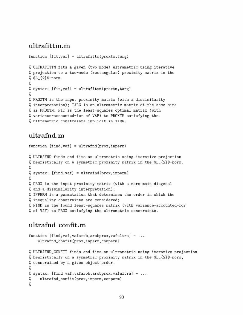
ultrafittm.m

function [fit,vaf] = ultrafittm(proxtm,targ)

% ULTRAFITTM fits a given (two-mode) ultrametric using iterative% projection to a two-mode (rectangular) proximity matrix in the% $L_{2}$-norm.%% syntax: [fit,vaf] = ultrafittm(proxtm,targ)%% PROXTM is the input proximity matrix (with a dissimilarity% interpretation); TARG is an ultrametric matrix of the same size% as PROXTM; FIT is the least-squares optimal matrix (with% variance-accounted-for of VAF) to PROXTM satisfying the% ultrametric constraints implicit in TARG.

ultrafnd.m

function [find,vaf] = ultrafnd(prox,inperm)

% ULTRAFND finds and fits an ultrametric using iterative projection% heuristically on a symmetric proximity matrix in the $L_{2}$-norm.%% syntax: [find,vaf] = ultrafnd(prox,inperm)%% PROX is the input proximity matrix (with a zero main diagonal% and a dissimilarity interpretation);% INPERM is a permutation that determines the order in which the% inequality constraints are considered;% FIND is the found least-squares matrix (with variance-accounted-for% of VAF) to PROX satisfying the ultrametric constraints.

ultrafnd confit.m

function [find,vaf,vafarob,arobprox,vafultra] = ...ultrafnd_confit(prox,inperm,conperm)

% ULTRAFND_CONFIT finds and fits an ultrametric using iterative projection% heuristically on a symmetric proximity matrix in the $L_{2}$-norm,% constrained by a given object order.%% syntax: [find,vaf,vafarob,arobprox,vafultra] = ...% ultrafnd_confit(prox,inperm,conperm)%

90

% PROX is the input proximity matrix (with a zero main diagonal% and a dissimilarity interpretation);% INPERM is a permutation that determines the order in which the% inequality constraints are considered in obtaining the ultrametric;% CONPERM is the given constraining object order;% VAFAROB is the VAF of the anti-Robinson matrix fit, AROBPROX, to PROX;% VAFULTRA is the VAF of the ultrametric fit to AROBPROX;% FIND is the found least-squares matrix (with variance-accounted-for% of VAF) to PROX satisfying the ultrametric constraints, and given% in CONPERM order.

ultrafnd confnd.m

function [find,vaf,conperm,vafarob,arobprox,vafultra] = ...ultrafnd_confnd(prox,inperm)

% ULTRAFND_CONFND finds and fits an ultrametric using iterative projection% heuristically on a symmetric proximity matrix in the $L_{2}$-norm, and% also locates a initial constraining object order.%% syntax: [find,vaf,conperm,vafarob,arobprox,vafultra] = ...% ultrafnd_confnd(prox,inperm)%% PROX is the input proximity matrix (with a zero main diagonal% and a dissimilarity interpretation);% INPERM is a permutation that determines the order in which the% inequality constraints are considered in obtaining the ultrametric;% CONPERM is the identified constraining object order;% VAFAROB is the VAF of the anti-Robinson matrix fit, AROBPROX, to PROX;% VAFULTRA is the VAF of the ultrametric fit to AROBPROX;% FIND is the found least-squares matrix (with variance-accounted-for% of VAF) to PROX satisfying the ultrametric constraints, and given% in CONPERM order.

ultrafnd missing.m

function [find,vaf] = ultrafnd_missing(prox,inperm,proxmiss)

% ULTRAFND_MISSING finds and fits an ultrametric using iterative projection% heuristically on a symmetric proximity matrix in the $L_{2}$-norm.%% syntax: [find,vaf] = ultrafnd_missing(prox,inperm,proxmiss)%% PROX is the input proximity matrix (with a zero main diagonal

91

% and a dissimilarity interpretation); also, missing entries in the input% proximity matrix PROX are given values of zero.% INPERM is a permutation that determines the order in which the% inequality constraints are considered;% FIND is the found least-squares matrix (with variance-accounted-for% of VAF) to PROX satisfying the ultrametric constraints. PROXMISS is% the same size as PROX (with main% diagonal entries all zero); an off-diagonal entry of 1.0 denotes an% entry in PROX that is present and 0.0 if it is absent.

ultrafndtm.m

function [find,vaf] = ultrafndtm(proxtm,inpermrow,inpermcol)

% ULTRAFNDTM finds and fits a two-mode ultrametric using% iterative projection heuristically on a rectangular proximity% matrix in the $L_{2}$-norm.%% syntax: [find,vaf] = ultrafndtm(proxtm,inpermrow,inpermcol)%% PROXTM is the input proximity matrix (with a% dissimilarity interpretation);% INPERMROW and INPERMCOL are permutations for the row and column% objects that determine the order in which the% inequality constraints are considered;% FIND is the found least-squares matrix (with variance-accounted-for% of VAF) to PROXTM satisfying the ultrametric constraints.

ultraorder.m

function [orderprox,orderperm] = ultraorder(prox)

% ULTRAORDER finds for the input proximity matrix PROX% (assumed to be ultrametric with a zero main diagonal)% a permutation ORDERPERM that displays the anti-% Robinson form in the reordered proximity matrix% ORDERPROX; thus, prox(orderperm,orderperm) = orderprox.%% syntax: [orderprox,orderperm] = ultraorder(prox)

ultraplot.m

function [] = ultraplot(ultra)

92

% ULTRAPLOT gives a dendrogram plot for the input ultrametric% dissimilarity matrix ULTRA.%% syntax: [] = ultraplot(ultra)

93

cluster analysis: a toolbox for...

Documents