Clouds, Precipitation, and Marine Boundary Layer Structure duringthe MAGIC Field Campaign

XIAOLI ZHOU AND PAVLOS KOLLIAS

Department of Atmospheric and Oceanic Sciences, McGill University, Montreal, Quebec, Canada

ERNIE R. LEWIS

Biological, Environmental and Climate Sciences Department, Brookhaven National Laboratory, Upton, New York

(Manuscript received 2 May 2014, in final form 16 December 2014)

ABSTRACT

The recent ship-basedMarine ARMGCSS Pacific Cross-Section Intercomparison (GPCI) Investigation of

Clouds (MAGIC) field campaign with the marine-capable Second ARM Mobile Facility (AMF2) deployed

on the Horizon Lines cargo container M/V Spirit provided nearly 200 days of intraseasonal high-resolution

observations of clouds, precipitation, and marine boundary layer (MBL) structure on multiple legs between

Los Angeles, California, and Honolulu, Hawaii. During the deployment, MBL clouds exhibited a much

higher frequency of occurrence than other cloud types and occurredmore often in thewarm season than in the

cold season.MBL clouds demonstrated a propensity to produce precipitation, which often evaporated before

reaching the ocean surface. The formation of stratocumulus is strongly correlated to a shallow MBL with

a strong inversion and a weak transition, while cumulus formation is associated with a much weaker inversion

and stronger transition. The estimated inversion strength is shown to depend seasonally on the potential

temperature at 700 hPa. The location of the commencement of systematic MBL decoupling always occurred

eastward of the locations of cloud breakup, and the systematic decoupling showed a strong moisture strati-

fication. The entrainment of the dry warm air above the inversion appears to be the dominant factor triggering

the systematic decoupling, while surface latent heat flux, precipitation, and diurnal circulation did not play

major roles. MBL clouds broke up over a short spatial region due to the changes in the synoptic conditions,

implying that in real atmospheric conditions the MBL clouds do not have enough time to evolve as in the

idealized models.

1. Introduction

On average, near 30% of the global oceans are cov-

ered with low-level clouds [see the International Satel-

lite Cloud Climatology Project (ISCCP) online dataset,

at http://isccp.giss.nasa.gov/climanal7.html]. These pre-

vailing marine boundary layer (MBL) clouds are a key

component in Earth’s radiation budget, from which

stratocumulus (Sc) clouds exert a strong negative net

radiative effect due to their low height and high areal

coverage, by strongly reflecting incoming solar radiation

but only weakly influencing the outgoing longwave ra-

diation (Wood 2012). Cumulus (Cu) have a reduced

effect on the radiation due to their low areal coverage

(Wood 2012; Karlsson et al. 2010) but play a critical role

in the vertical redistribution of moisture and energy in

the lower troposphere (Tiedtke et al. 1988). Thus, it is

important for global climate models to accurately rep-

resent these cloud regimes.

The evolution, with increasing sea surface tempera-

ture (SST), from Sc regimes to Cu regimes in the trade

wind regions and then eventually to congestus and deep

convective Cuover thewarmerwaters of the intertropical

convergence zone is well documented (e.g., Albrecht

et al. 1995a,b; Karlsson et al. 2010). An inversion layer

that is often thought of as the top of the MBL typically

caps the Sc. A regime with Cu under Sc usually occurs

during the progression between Sc and Cu and is associ-

ated with a weakly stable layer below the inversion base

that is characterized by a sharp decrease of moisture with

height (e.g., Krueger et al. 1995; Bretherton and Wyant

Corresponding author address: Xiaoli Zhou, Department of

Atmospheric and Oceanic Sciences, Burnside Hall, Room 945, 805

Sherbrooke Street West, Montreal QC H3A0B9, Canada.

E-mail: xiaoli.zhou@mail.mcgill.ca

2420 JOURNAL OF CL IMATE VOLUME 28

DOI: 10.1175/JCLI-D-14-00320.1

� 2015 American Meteorological Society

BNL-107366-2015-JA

1997; Jones et al. 2011). This stable layer, referred here

as the transition layer, separates a region below of sur-

face flux–driven turbulence from a region above domi-

nated by radiatively driven convection (Bretherton and

Wyant 1997) and acts to isolate the upperMBL from the

surface moisture supply. When this vertical moisture

stratification gets sufficiently strong, systematic decoupling

occurs and the MBL remains decoupled with further in-

crease in SST. This systematic decoupling is a crucial first

step in the Sc-to-Cu transition and is not affected by the

diurnal cycle of radiation (Wyant et al. 1997).

Because of the lack of full understanding of the mech-

anisms responsible for the evolution of MBL structure

and clouds, global weather and climate prediction models

still do not accurately reproduce the evolution between

these cloud regimes, and the locations of Sc breakup and

the rates of change of cloud coverage vary widely among

different models, which generally underestimate cloud

amounts in the Sc region while overestimating them in the

Cu region (Teixeira et al. 2011).

One of the main factors hindering progress in repre-

senting these clouds in numerical models has been the lack

of observational data. Most of the observational datasets

used to evaluate the cloud-related processes are satellite

based. Satellite data have proven valuable in determining

the climatological links between MBL inversion base

height (MBLH) and cloud cover (e.g., Heck et al. 1990;

Wang et al. 1993; Wood and Bretherton 2004). However,

satellite observations cannot provide information on de-

tailed vertical cloud and thermodynamic structure of the

MBL especially during decoupling conditions (Wood and

Bretherton 2004; Karlsson et al. 2010). The difficulty in

accurately observing low-level clouds with small-scale

variability (Xu and Cheng 2013) further restricts the ap-

plicability of satellite data in the understanding of the

transition between these cloud regimes.

In addition to satellite data, several field campaigns

have been conducted to study MBL clouds and the

mechanisms responsible for the Sc-to-Cu transition.

These previous ship- or aircraft-based efforts provided a

wealth of information with regard to the vertical structure

of the MBL and associated clouds. However, they were

primarily conducted in a fairly small region and focused

on studying one specific cloud type. For example, the

First ISCCP Regional Experiment (FIRE; Albrecht

et al. 1988) focused on Sc and cirrus cloud regimes; the

Tropical InstabilityWave Experiment (TIWE; Albrecht

et al. 1995b) focused on the trade wind Cu boundary

layer structure; and during the Atlantic Stratocumulus

Transition Experiment (ASTEX; Albrecht et al. 1995a)

a transition region in which Cu form beneath Sc was

observed. Albrecht et al. (1995b) compared the large-

scale forcing and thermodynamic profiles from these

three field experiments and concluded that the increase

in SST is important in the thinning of the Sc. The same

study provided evidence that the boundary layer struc-

ture and the associated transition from Sc to Cu may be

more complicated than originally thought. More re-

cently, Jones et al. (2011) examined in detail the coupled

and decoupled boundary layers in the Variability of

the American Monsoon Systems (VAMOS) Ocean–

Cloud–Atmosphere–Land Study Regional Experiment

(VOCALS-REx; Wood et al. 2011). One of the major

findings in Jones et al. (2011) is that the difference

between MBLH and the lifting condensation level

(LCL) best predicts decoupling.

Previous numerical studies have demonstrated that

the systematic decoupling is mainly driven by the in-

creasing surface latent heat flux (LHF) as a response to

the increasing entrainment due to the warmer SST (e.g.,

Bretherton and Wyant 1997; Sandu and Stevens 2011).

The subsequent Sc breakup was explained as a result of

the further increase of the SST that causes the Cu to be-

come deeper and more vigorous, penetrating farther into

the inversion and entraining more dry air from above the

inversion (Wyant et al. 1997; Sandu and Stevens 2011).

Although numerical studies have advanced our knowl-

edge of MBL structure and clouds, simulations have

usually simplified the problem by assuming the constant

divergence and free-tropospheric lapse rates (Bretherton

and Wyant 1997), but neither assumption is supported by

observations.

There are noticeable discrepancies between idealized

model simulations and observational findings. For in-

stance, the dominant effect of the LHF on MBL decou-

pling was not observed in VOCAL-REx (Jones et al.

2011). Additionally, the assumption of a constant free-

atmosphere lapse rate might introduce biases because

MBLH and boundary layer mixing ratios are very

sensitive to above-inversion features (Albrecht 1984;

Krueger et al. 1995). At the same time, the availability

of comprehensive, long-term observations that docu-

ment the gradual MBL decoupling and Sc-to-Cu tran-

sitions is limited.

The recent Marine ARM GCSS Pacific Cross-Section

Intercomparison (GPCI) Investigation of Clouds (MAGIC)

field campaign provided high-resolution profiling ob-

servations from the coast of California to Honolulu for

over 200 days. The collected dataset is the most ex-

tensive direct, long-term, intraseasonal set of mea-

surements of MBL structure and cloud evolution from

Sc to Cu over large downwind regions. Here, we in-

vestigate the potential of the dataset in advancing our

understanding of the systematic MBL decoupling and

Sc breakup to be compared with and constrain the

modeling studies.

15 MARCH 2015 ZHOU ET AL . 2421

The remainder of the manuscript is organized as fol-

lows. Brief descriptions of the MAGIC field campaign

and of the Second ARM Mobile Facility (AMF2) in-

struments are provided in section 2, and themethodology

used for this study is introduced in section 3. Results are

presented in section 4, and a summary of these results and

plans for future work are presented in section 5.

2. Observations

a. The MAGIC field campaign

The MAGIC field campaign (http://www.arm.gov/

sites/amf/mag/) deployed the U.S. Department of En-

ergy (DOE) Atmospheric Radiation Measurement

Program Mobile Facility 2 (AMF2) on the commercial

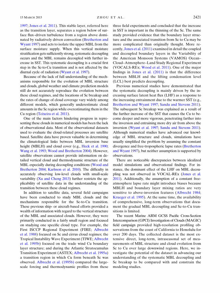
cargo container shipHorizon Spirit (Fig. 1a). TheMAGIC

transect is very near the line from the coast of California

to the equator (358N, 1258W to 18S, 1738W) that was

chosen by modelers to compare model results for the

Global Energy and Water Experiment (GEWEX)

Cloud System Studies (GCSS) Pacific Cross-Section

Intercomparison (GPCI) study, in which more than

20 climate and weather-prediction models participated

(Teixeira et al. 2011).Thus,MAGICwith its unprecedented,

intraseasonal, high-resolution ship-based observations is

expected to provide constraint, validation, and support

for the aforementionedmodeling efforts and at the same

time contribute in improving our understanding of the

Sc-to-Cu transition along this GPCI transect.

From October 2012 through September 2013, the

Spirit completed 20 round trips between Los Angeles,

California, and Honolulu, Hawaii. Each trip is called

a ‘‘leg,’’ and legs are numbered sequentially as ‘‘LegxxA’’

for the trips from Los Angeles to Honolulu and

‘‘LegxxB’’ for the return trips (Fig. 1b). During the legs

from Los Angeles, the Spirit traveled at ;21kt

(;10.5ms21; 1 kt5 0.51ms21) and covered the 4100-km

distance in 4.5 days. The Spirit returned to Los Angeles

at ;16 kt (;8m s21), making the trip in approximately

6.5 days (the lower speed resulting in lower fuel costs

and allowing the ship to remain on a two-week sched-

ule; Lewis et al. 2012). The departure and arrival times

of MAGIC legs are listed in appendix A. Two techni-

cians associated with the MAGIC campaign lived on

FIG. 1. (a) Horizon Spirit showing location of the bridge regionwhere theAMF2was located. (b) Tracks ofMAGIC

legs between California and Hawaii (red lines) and great circle route (blue line).

2422 JOURNAL OF CL IMATE VOLUME 28

board the Spirit during the deployment to maintain

the instrumentation, launch radiosondes, and perform

other tasks.

b. AMF2 instrumentation and data description

The AMF2 contains a state-of-the-art instrumentation

suite and was designed to operate in a wide range of cli-

mate conditions and locations, including shipboard de-

ployments. The AMF2 was located on the bridge deck

of the Spirit, approximately 16m above mean sea level

(MSL). The primary AMF2 instruments used in the cur-

rent study are 1) a Ka-band ARM zenith radar (KAZR),

2) a laser ceilometer, 3) a Vaisala weather station, 4) an

inertial navigational location and attitude system (NAV),

5) the Marine Meteorological System (MARMET) in-

stalled on the mast of the Spirit approximately 27m

above sea level and an Infrared SST Autonomous Ra-

diometer (ISAR), and 6) radiosondes (four or eight per

day). AMF2 also contained a motion-stabilized W-band

radar, a radar wind profiler, a broadband and spectral

radiometer suite, aerosol instrumentation, and other

instruments. The operational status of all instruments

during the campaign is summarized in appendix B.

There were some time periods when the KAZR was not

acquiring data for various reasons (e.g., installation,

power outages, etc.), but KAZR measurements were

obtained for all of Leg03A through Leg08B, Leg11, and

Leg14A through Leg17B. The analyses presented here

are based on these data, in total 22 transits between

California and Hawaii through the Sc-to-Cu transition

region comprising more than 3000 h. The data are sep-

arated into two seasons: the warm season, Leg11 and

Leg14 to Leg17 (25 May–6 June and 7 July–29 August

2013), and the cold season, Leg03 to Leg08 (6 October–

27 December 2012).

1) KA-BAND ARM ZENITH RADAR

The KAZR, formerly known as the millimeter

wavelength cloud radar (MMCR; Moran et al. 1998), is

a 35-GHz profiling Doppler radar that retrieves in-

formation on the vertical distribution of the hydrome-

teors in the atmospheric column. Because of its short

wavelength (8.6mm), the KAZR has sufficient sensi-

tivity to detect MBL clouds with little attenuation under

moderate drizzle conditions. The KAZR might fail to

detect very thin liquid clouds and it can provide in-

accurate hydrometeor-layer heights during heavy pre-

cipitation because of severe radar signal attenuation

(Matrosov 2007), but because a ceilometer was used

[section 2b(2)] and because there was very little heavy

precipitation during MAGIC, these issues should have

little effect on the results of this study. The KAZR uti-

lizes a new digital receiver that provides higher temporal

(less than 2 s) and spatial (30m) resolution than the

MMCR (Widener et al. 2012). It is unaffected by Bragg

scattering and has small antennaswith narrow beamwidths

as well as limited sidelobes (Kollias et al. 2007). During

MAGIC, the KAZR was configured to have temporal

resolution of about 0.4 s to oversample the ship motion,

thus enabling compensation of the effects of this mo-

tion on the radar observables during data post-

processing. In this study, all KAZR measurements

have been averaged over 4 s, which allows for the de-

tection of small-scale Cu.

2) CEILOMETER

A ceilometer (Vaisala model CT25K) operating at

a wavelength of 910nm was used to detect the base

heights of clouds. The ceilometer’s range resolution was

10m, and its temporal resolution was near 16 s for Leg03

and Leg04 and 3 s for the other legs. To maintain the 4-s

temporal resolution, it is assumed that each reported

base height is representative of the entire original time

period.

3) VAISALA WEATHER STATION

AVaisala weather stationWXT-520 installed as part of

a suite of meteorological instruments associated with the

Aerosol Observing System of the AMF2 (AOSMET)

measured rain intensity at 1-s resolution, which was used

to detect the presence of precipitation reaching the

ground (see section 3c).

4) NAVIGATIONAL LOCATION AND ATTITUDE

NAV provided ship location and attitude with a tem-

poral resolution of 1 s during the period between No-

vember 3 and 3December 2012 (Leg05A to Leg07A), and

0.1 s for the rest of the deployment. As all macroscopic

data are averaged over 4 s, both temporal resolutions are

sufficiently accurate for the present comparisons.

5) MARINE METEOROLOGICAL MEASUREMENT

AND MARINE FLUX DATASETS

TheMARMETXdataset (http://www.arm.gov/campaigns/

amf2012magic/) contains standard surfacemeteorological

parameters measured by the MARMET: temperature

(T), pressure (P), relative humidity (RH), and apparent

and true wind speed and direction; and the sea surface

skin temperature (SSST) measured by the ISAR (with

an accuracy of better than 0.18C). The Marine Flux

dataset (MARFLUX; http://www.arm.gov/campaigns/

amf2012magic/) contains the surface fluxes of moisture

and sensible and latent heat calculated by the TOGA

COARE air–sea flux algorithm (Fairall et al. 1996)

using the MARMETX variables. Both MARMETX

and MARFLUX have a time resolution of 1min.

15 MARCH 2015 ZHOU ET AL . 2423

6) ATMOSPHERIC SOUNDINGS

Standard radiosondes (Vaisala model MW-31, SN

E50401) were launched every 6 h to measure vertical

profiles of the thermodynamic state of the atmosphere

(T, P, RH, and wind speed and direction). During

Leg14, which occurred in July 2013, launches weremade

every 3 h to provide a more detailed picture of the at-

mospheric structure. Only soundings providing mea-

surements as high as 15 km were used in this study (389

in all). The radiosondes collected data every 2 s during

their ascent, providing a typical vertical resolution of

10m in the troposphere. However, owing to the limited

launching frequency (four to eight per day), sounding

data can be interpolated to higher-resolution time steps

with only limited confidence.

3. Methodology

a. Hydrometeor mask

A hydrometer mask was applied to the raw KAZR

reflectivity measurements to identify the radar range

gates that contain appreciable returns from hydrome-

teors. Following Rémillard et al. (2012), this mask uses

the algorithm of Hildebrand and Sekhon (1974) and

a two-dimensional (time–height) filter to identify the

number of hydrometeor layers in the atmospheric col-

umn and their corresponding boundaries. The lowest

hydrometeor boundary is not necessarily the cloud base

because the KAZR cannot distinguish cloud drops from

precipitation particles below the cloud base.

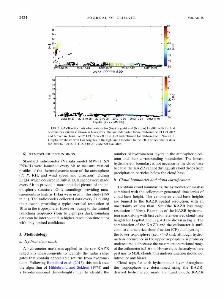
b. Cloud boundaries and cloud classification

To obtain cloud boundaries, the hydrometeor mask is

combined with the ceilometer-generated time series of

cloud-base height. The ceilometer cloud-base heights

are binned to the KAZR spatial resolution, with an

uncertainty of less than 15m (the KAZR has range

resolution of 30m). Examples of the KAZR hydrome-

teor mask along with first ceilometer-derived cloud-base

heights for Leg04A and Leg04B are shown in Fig. 2. The

combination of the KAZR and the ceilometer is suffi-

cient to characterize cloud fraction (CF) and layering in

the lower troposphere (i.e., ,;3 km), although hydro-

meteor occurrence in the upper troposphere is probably

underestimated because the maximum operational range

of the ceilometer is 5–6km.However, as the analysis here

pertains to MBL clouds, this underestimation should not

introduce any biases.

Cloud tops for each hydrometeor layer throughout

the troposphere are determined using the KAZR-

derived hydrometeor mask. In liquid clouds, KAZR

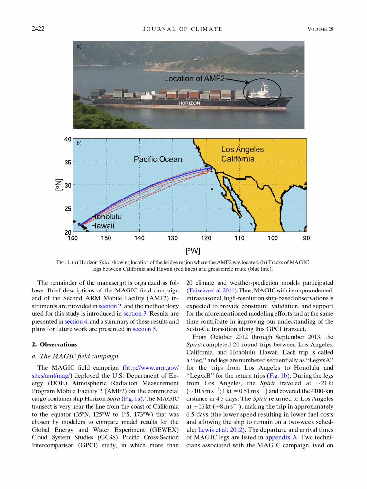
FIG. 2. KAZR reflectivity observations for (top) Leg04A and (bottom) Leg04B with the first

ceilometer cloud base shown as black dots. The Spirit departed from California on 21 Oct 2012

and arrived in Hawaii on 25 Oct, then left on 26 Oct and returned to California on 1 Nov 2012.

Graphs are shown with Los Angeles to the right and Honolulu to the left. The ceilometer data

for 0000 to ;2116 UTC 22 Oct 2012 are not available.

2424 JOURNAL OF CL IMATE VOLUME 28

reflectivitymeasurements below the first cloud-base height

determined by the ceilometer are used to characterize

precipitation (see next section). If no ceilometer data are

available, noKAZRdata below 300m are used, since they

often contain artifacts (especially when no precipitation is

present). In cases when the first ceilometer-derived base

height is 100m or more less than the first KAZR-defined

hydrometeor base height, the two clouds are considered

independent, with the first cloud-top height undetermined;

otherwise the first KAZR hydrometeor top is considered

to be the first cloud top.

Once the cloud boundaries are determined, each

time–height cluster of KAZR echoes with more than

25 connected pixels (in time–height space) is considered

to be a cloud entity. To obtain realistic bases of multiple-

layer cloud entities, the bases of the second cloud level

are further smoothed according to the ceilometer-

derived base heights. KAZR echoes below the newly

defined cloud bases are neglected. Each cloud entity is

categorized into one of four types based on its average

base and top heights (Table 1; see Fig. 3a as an example):

high-level, midlevel, MBL, or cumulus congestus and

deep convective. High-level clouds have average base

heights of at least 6 km. Midlevel clouds have average

base heights between 3 and 6km. MBL clouds have

average base heights and top heights less than 3km, or

have undetermined average top heights. Cumulus con-

gestus and deep convective clouds have average base

heights less than 3km but average top heights of at least

3 km. The statistical results of cloud properties pre-

sented in this study are not sensitive to the specific

values chosen for the thresholds.

An MBL cloud layer is detected if more than 10% of

cloud bases are measured over a continuous range of

heights during 1h (a one-gate gap is allowed). The cloud

bases here refer to the first and second ceilometer-derived

bases and the first three hydrometeor-mask bases.

As the focus of this study is MBL clouds, emphasis is

placed on these clouds, which are further divided into three

subtypes: stratocumulus, cumulus, and indeterminate (e.g.,

Figs. 3b and 3c). Sc are low clouds composed of an en-

semble of individual convective elements that together

assume a layered form (Wood 2012), whereas Cu clouds

are separate convective elements. The difference be-

tween Sc and Cu in this study is based on their time

durations: a cloud is defined as Sc if it lasts more than

20min, and as Cu if its duration is less than 20min. Sc

clouds are also required to have a narrow cloud-top

height distribution that is restricted by a specific stan-

dard deviation threshold that depends on its duration

(see Table 1 for details). The remaining MBL cloud

clusters make up the subtype ‘‘indeterminate.’’ Because

of the limited nature of theMAGIC observations (1D in

distance/time and height), these cloud types are not

mutually exclusive.

Because of their ship-based origin, the cloud macro-

scopic data for each leg depend on both time and location

(e.g., Figs. 1 and 2). To account for slight ship-course

deviations between different legs (Fig. 1b), all of the

cloud macroscopic data are binned to a uniform great-

circle route with 40-m resolution (the approximate dis-

tance covered by the ship in 4 s) in order to examine the

evolution of cloud properties along this representative

great-circle transect. Finally, all the cloud macroscopic

data are averaged over 36 km (the approximate distance

covered by the ship in 1 h) and converted to the corre-

sponding latitude along the great-circle route. The fre-

quency of occurrence of MBL cloud every 36km are

considered to represent the CF over that area and are

referred to as CF36 in this paper.

c. Precipitation classification

KAZR observations, the KAZR-derived hydrometer

mask, ceilometer-derived cloud-base heights, surface

rainfall occurrence from the weather stations, and 08Cisotherm heights derived from interpolated radiosonde

data are used characterize precipitation. KAZR echoes

are classified as either cloud or precipitation; no attempt

is made to distinguish ice hydrometeors from liquid

cloud drops or precipitation. Because the cloud-base

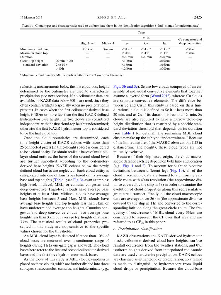
TABLE 1. Cloud types and characteristics used to differentiate them in the identification algorithm (‘‘Ind’’ stands for indeterminate).

Type

High level Midlevel

MBL Cu congestus and

deep convectiveSc Cu Ind

Minimum cloud base $6 km 3–6 km ,3 km* ,3 km* ,3 km* ,3 km

Maximum cloud top — — ,3 km ,3 km ,3 km $3 km

Duration — — $20min ,20min $20min —

Cloud-top height

standard deviation

20min to 2 h — — ,100m — $100m —

2 to 10 h — — ,160m — $160m —

.10 h — — ,200m — $200m —

*Minimum cloud base for MBL clouds is either below 3 km or undetermined.

15 MARCH 2015 ZHOU ET AL . 2425

heights are determined from the ceilometer data, every

KAZR echo below the first cloud-base height is classi-

fied as precipitation. The ceilometer quality control flag

was checked to ensure that no water was present on the

ceilometer window (which would occur in the case of

intense precipitation reaching the surface), since this

would strongly attenuate the signal and result in in-

accurate readings.

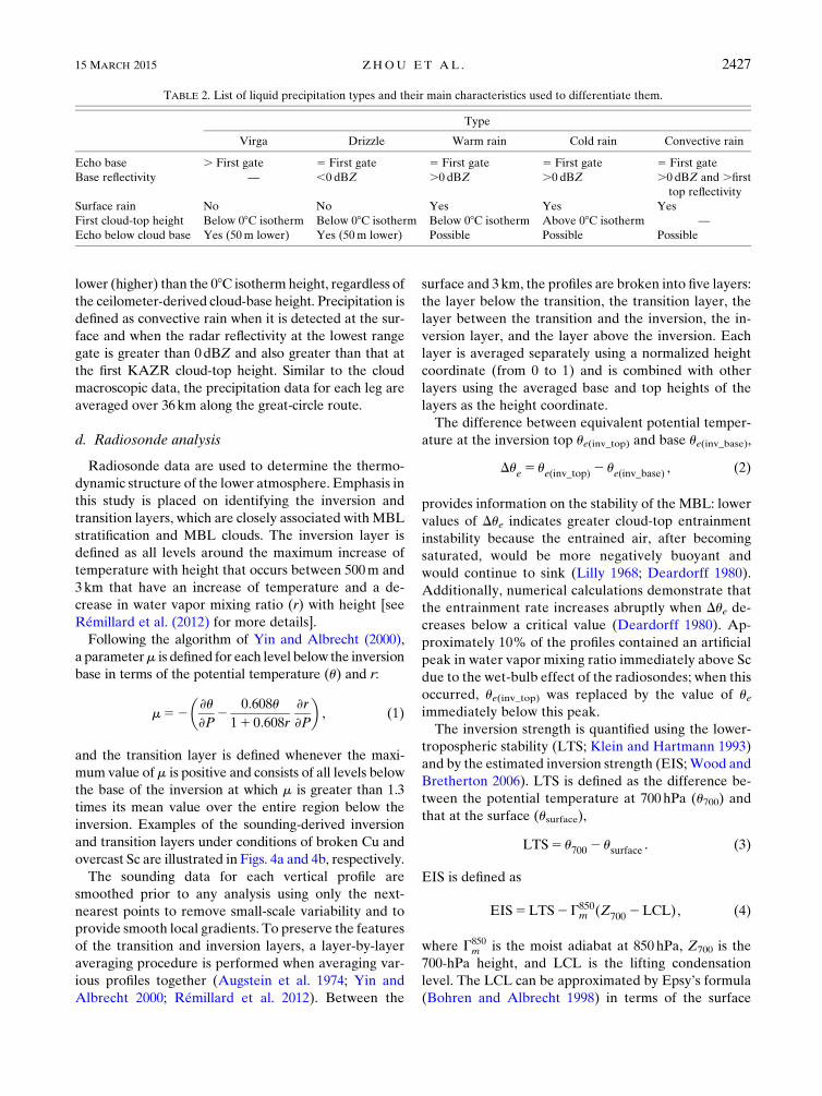
Precipitation is classified into five types (Table 2):

virga, drizzle, warm rain, cold rain, and deep convective

rain (e.g., Fig. 3d). Precipitation that is not detected at

the surface is either virga or drizzle. The distinction

between the two is based on the detection of KAZR

echoes in the lowest range gate (around 120m ASL

before Leg11A, and 240m ASL for the later legs): virga

is defined as precipitation that is detected at least 50m

below the ceilometer cloud base and does not reach the

lowest KAZR range gate, whereas drizzle is detected at

the KAZR lowest range gate. This distinction provides

a qualitative indicator of light rain intensity and indicates

the portion of the subcloud layer affected by evaporation.

Under this proposed definition only rain that falls

through a cloud and not that from the side of a cloud

could be considered virga. Precipitation is defined as

warm (cold) rain when it is detected at the surface and

when the first KAZR-derived cloud top is above 3kmbut

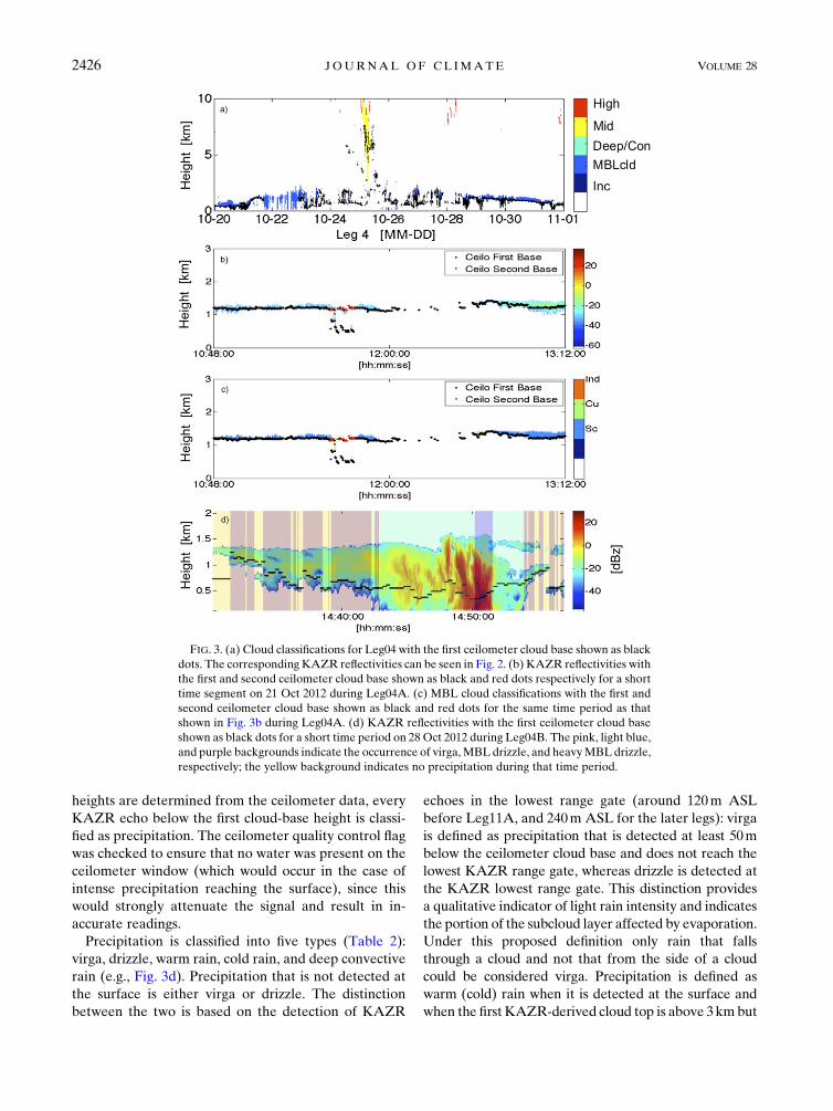
FIG. 3. (a) Cloud classifications for Leg04 with the first ceilometer cloud base shown as black

dots. The corresponding KAZR reflectivities can be seen in Fig. 2. (b) KAZR reflectivities with

the first and second ceilometer cloud base shown as black and red dots respectively for a short

time segment on 21 Oct 2012 during Leg04A. (c) MBL cloud classifications with the first and

second ceilometer cloud base shown as black and red dots for the same time period as that

shown in Fig. 3b during Leg04A. (d) KAZR reflectivities with the first ceilometer cloud base

shown as black dots for a short time period on 28 Oct 2012 during Leg04B. The pink, light blue,

and purple backgrounds indicate the occurrence of virga,MBL drizzle, and heavyMBL drizzle,

respectively; the yellow background indicates no precipitation during that time period.

2426 JOURNAL OF CL IMATE VOLUME 28

lower (higher) than the 08C isotherm height, regardless of

the ceilometer-derived cloud-base height. Precipitation is

defined as convective rain when it is detected at the sur-

face and when the radar reflectivity at the lowest range

gate is greater than 0dBZ and also greater than that at

the first KAZR cloud-top height. Similar to the cloud

macroscopic data, the precipitation data for each leg are

averaged over 36km along the great-circle route.

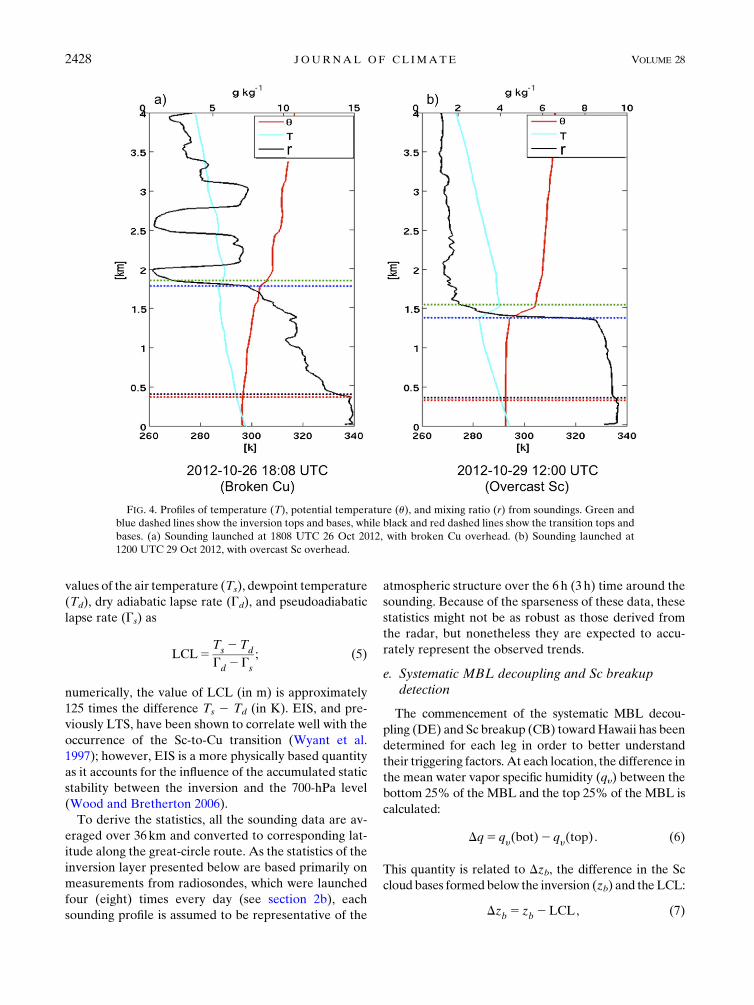
d. Radiosonde analysis

Radiosonde data are used to determine the thermo-

dynamic structure of the lower atmosphere. Emphasis in

this study is placed on identifying the inversion and

transition layers, which are closely associated with MBL

stratification and MBL clouds. The inversion layer is

defined as all levels around the maximum increase of

temperature with height that occurs between 500m and

3km that have an increase of temperature and a de-

crease in water vapor mixing ratio (r) with height [see

Rémillard et al. (2012) for more details].

Following the algorithm of Yin and Albrecht (2000),

a parameterm is defined for each level below the inversion

base in terms of the potential temperature (u) and r:

m52

�›u

›P2

0:608u

11 0:608r

›r

›P

�, (1)

and the transition layer is defined whenever the maxi-

mum value ofm is positive and consists of all levels below

the base of the inversion at which m is greater than 1.3

times its mean value over the entire region below the

inversion. Examples of the sounding-derived inversion

and transition layers under conditions of broken Cu and

overcast Sc are illustrated in Figs. 4a and 4b, respectively.

The sounding data for each vertical profile are

smoothed prior to any analysis using only the next-

nearest points to remove small-scale variability and to

provide smooth local gradients. To preserve the features

of the transition and inversion layers, a layer-by-layer

averaging procedure is performed when averaging var-

ious profiles together (Augstein et al. 1974; Yin and

Albrecht 2000; Rémillard et al. 2012). Between the

surface and 3km, the profiles are broken into five layers:

the layer below the transition, the transition layer, the

layer between the transition and the inversion, the in-

version layer, and the layer above the inversion. Each

layer is averaged separately using a normalized height

coordinate (from 0 to 1) and is combined with other

layers using the averaged base and top heights of the

layers as the height coordinate.

The difference between equivalent potential temper-

ature at the inversion top ue(inv_top) and base ue(inv_base),

Due 5 ue(inv_top) 2 ue(inv_base) , (2)

provides information on the stability of the MBL: lower

values of Due indicates greater cloud-top entrainment

instability because the entrained air, after becoming

saturated, would be more negatively buoyant and

would continue to sink (Lilly 1968; Deardorff 1980).

Additionally, numerical calculations demonstrate that

the entrainment rate increases abruptly when Due de-creases below a critical value (Deardorff 1980). Ap-

proximately 10% of the profiles contained an artificial

peak in water vapor mixing ratio immediately above Sc

due to the wet-bulb effect of the radiosondes; when this

occurred, ue(inv_top) was replaced by the value of ueimmediately below this peak.

The inversion strength is quantified using the lower-

tropospheric stability (LTS; Klein and Hartmann 1993)

and by the estimated inversion strength (EIS; Wood and

Bretherton 2006). LTS is defined as the difference be-

tween the potential temperature at 700hPa (u700) and

that at the surface (usurface),

LTS5 u7002 usurface . (3)

EIS is defined as

EIS5LTS2G850m (Z700 2LCL), (4)

where G850m is the moist adiabat at 850 hPa, Z700 is the

700-hPa height, and LCL is the lifting condensation

level. The LCL can be approximated by Epsy’s formula

(Bohren and Albrecht 1998) in terms of the surface

TABLE 2. List of liquid precipitation types and their main characteristics used to differentiate them.

Type

Virga Drizzle Warm rain Cold rain Convective rain

Echo base . First gate 5 First gate 5 First gate 5 First gate 5 First gate

Base reflectivity — ,0 dBZ .0 dBZ .0 dBZ .0 dBZ and .first

top reflectivity

Surface rain No No Yes Yes Yes

First cloud-top height Below 08C isotherm Below 08C isotherm Below 08C isotherm Above 08C isotherm —

Echo below cloud base Yes (50m lower) Yes (50m lower) Possible Possible Possible

15 MARCH 2015 ZHOU ET AL . 2427

values of the air temperature (Ts), dewpoint temperature

(Td), dry adiabatic lapse rate (Gd), and pseudoadiabatic

lapse rate (Gs) as

LCL5Ts 2Td

Gd 2Gs

; (5)

numerically, the value of LCL (in m) is approximately

125 times the difference Ts 2 Td (in K). EIS, and pre-

viously LTS, have been shown to correlate well with the

occurrence of the Sc-to-Cu transition (Wyant et al.

1997); however, EIS is a more physically based quantity

as it accounts for the influence of the accumulated static

stability between the inversion and the 700-hPa level

(Wood and Bretherton 2006).

To derive the statistics, all the sounding data are av-

eraged over 36 km and converted to corresponding lat-

itude along the great-circle route. As the statistics of the

inversion layer presented below are based primarily on

measurements from radiosondes, which were launched

four (eight) times every day (see section 2b), each

sounding profile is assumed to be representative of the

atmospheric structure over the 6 h (3 h) time around the

sounding. Because of the sparseness of these data, these

statistics might not be as robust as those derived from

the radar, but nonetheless they are expected to accu-

rately represent the observed trends.

e. Systematic MBL decoupling and Sc breakupdetection

The commencement of the systematic MBL decou-

pling (DE) and Sc breakup (CB) towardHawaii has been

determined for each leg in order to better understand

their triggering factors. At each location, the difference in

the mean water vapor specific humidity (qy) between the

bottom 25% of the MBL and the top 25% of the MBL is

calculated:

Dq5 qy(bot)2qy(top). (6)

This quantity is related to Dzb, the difference in the Sc

cloud bases formed below the inversion (zb) and theLCL:

Dzb 5 zb 2LCL, (7)

FIG. 4. Profiles of temperature (T), potential temperature (u), and mixing ratio (r) from soundings. Green and

blue dashed lines show the inversion tops and bases, while black and red dashed lines show the transition tops and

bases. (a) Sounding launched at 1808 UTC 26 Oct 2012, with broken Cu overhead. (b) Sounding launched at

1200 UTC 29 Oct 2012, with overcast Sc overhead.

2428 JOURNAL OF CL IMATE VOLUME 28

where zb is calculated as the maximum MBL cloud bases

(averaged over 36km) within four degrees longitude sur-

rounding each radiosonde. The linear relationship be-

tween Dq and Dzb (Fig. 5a) with the slope (276mkgg21)

and intercept (200m) comparable to those found in Jones

et al. (2011), demonstrate thatDq is a robust proxy forDzb.Some scatter is introduced since Dq comes from a single

profile while Dzb is an averaged maximum value. Biases

might be introduced when no Sc was detected near a ra-

diosonde or whenMBLHwas not well represented due to

the very shallow MBL near the coast of California. Thus

only those radiosondes within 1.5 standard deviations of

the least squares fit and that to the west of 1238W were

used (336 in total). A threshold of Dq . 1.5gkg21 (or

equivalently Dzi . 600m) is found appropriate to capture

the systematic decoupledMBL (Fig. 5b). Compared to the

threshold of Dq. 0.5gkg21 (Dzi . 150m) for all kinds of

decoupling in VOCAL-REx (Jones et al. 2011), the sys-

tematic decoupling showed much stronger moisture

stratification below the inversion. Subsequently, the DE

during each transect is then defined as the most easterly

profile of a group of profiles with continuous decoupling

features (Dq . 1.5 gkg21). Between the detected and the

nearest east radiosonde launches, the Dq criteria for de-

coupling is replaced by the difference of the instantaneous

ceilometer-derived cloud base height and LCL calculated

by the ship-measured T and RH. Compared to the sys-

tematic decoupling, the weak decoupled MBL is also

studied in this paper and is defined as theMBLwith Dzi.150m [consistent with Jones et al. (2011)].

Because of mesoscale influences, CF36 sometimes shows

variability and does not represent well the major cloud

evolution along the transect. To reduce the effects of me-

soscale variability and to more objectively capture CB, the

frequency of occurrence of the MBL clouds was averaged

over 108km (CF108). CB is then defined as the location

along the transect from California to Hawaii where CF108decreased from being greater than 80% for at least three

continuous points (324km) east of 1308Wtobeing less than

15%. Values of CF108 were generally not sensitive to the

above criteria. No cloud breakup points are determined if

values of CF108 east of 1308W were not sufficiently high

(Leg06A, Leg06B, Leg08A, Leg08B, and Leg17B) or if

they did not become sufficiently low (Leg15B). Those legs

FIG. 5. (a) The scatterplot of radiosonde-derived Dq for all the legs andmaximumDzbwithinfour degrees longitude surrounding each radiosonde. The solid black line is the least squares fit

with slope 276m kg g21 and intercept 200m. The dashed black line represents the thermody-

namic argument derived in Jones et al. (2011). The red dots indicate outliers outside 1.5

standard deviations of the least squares fit. (b) Radiosonde-derived Dq for all the legs along the

normalized path from California to DE to Hawaii.

15 MARCH 2015 ZHOU ET AL . 2429

are associated with either midlatitude or tropical cyclones,

or very strong cloud outbreaks thus do not represent the Sc

breakup in a general sense, and their exclusion helps to

elucidate the more general aspects of the transition.

4. Results

The results presented below are separated into two sec-

tions. The first section includes general statistical description

of MBL clouds, precipitation, thermodynamics, and their

seasonal behavior. The second section focuses on the study

of MBL systematic decoupling and cloud breakup.

a. General statistics of MBL clouds, precipitation, andthermodynamics

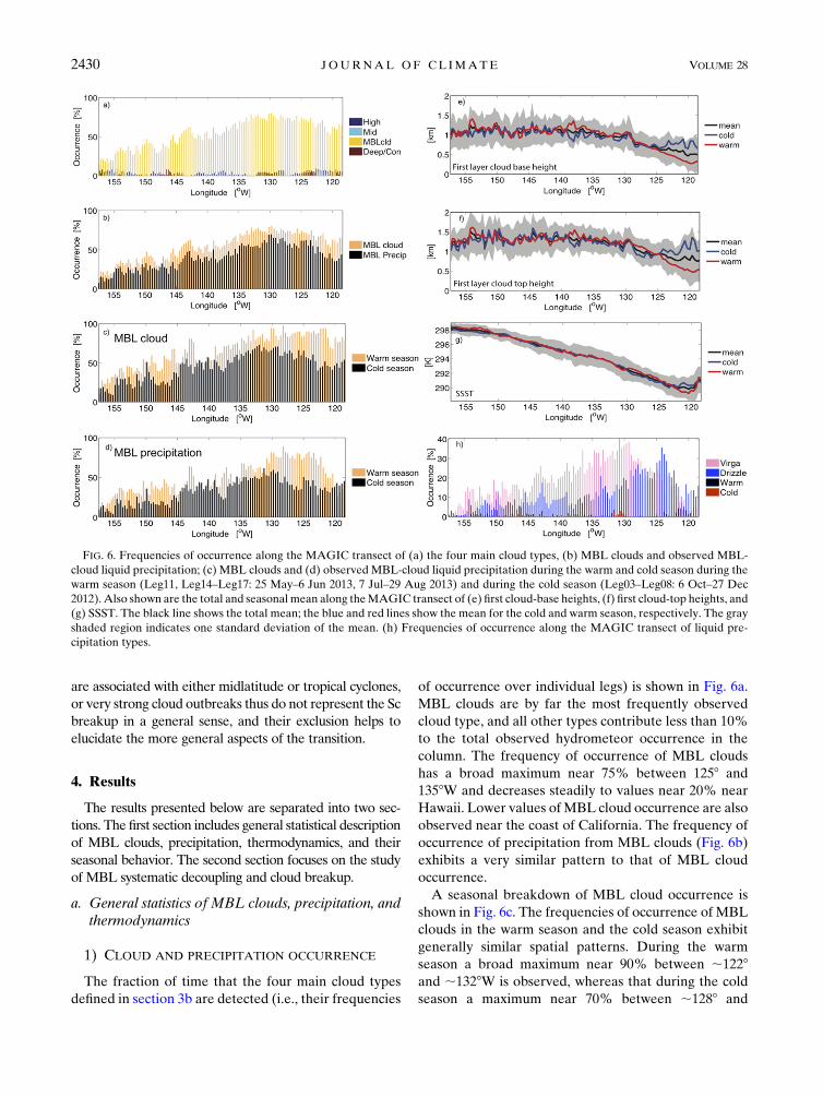
1) CLOUD AND PRECIPITATION OCCURRENCE

The fraction of time that the four main cloud types

defined in section 3b are detected (i.e., their frequencies

of occurrence over individual legs) is shown in Fig. 6a.

MBL clouds are by far the most frequently observed

cloud type, and all other types contribute less than 10%

to the total observed hydrometeor occurrence in the

column. The frequency of occurrence of MBL clouds

has a broad maximum near 75% between 1258 and

1358W and decreases steadily to values near 20% near

Hawaii. Lower values ofMBL cloud occurrence are also

observed near the coast of California. The frequency of

occurrence of precipitation from MBL clouds (Fig. 6b)

exhibits a very similar pattern to that of MBL cloud

occurrence.

A seasonal breakdown of MBL cloud occurrence is

shown in Fig. 6c. The frequencies of occurrence of MBL

clouds in the warm season and the cold season exhibit

generally similar spatial patterns. During the warm

season a broad maximum near 90% between ;1228and ;1328W is observed, whereas that during the cold

season a maximum near 70% between ;1288 and

FIG. 6. Frequencies of occurrence along the MAGIC transect of (a) the four main cloud types, (b) MBL clouds and observed MBL-

cloud liquid precipitation; (c) MBL clouds and (d) observed MBL-cloud liquid precipitation during the warm and cold season during the

warm season (Leg11, Leg14–Leg17: 25 May–6 Jun 2013, 7 Jul–29 Aug 2013) and during the cold season (Leg03–Leg08: 6 Oct–27 Dec

2012). Also shown are the total and seasonal mean along theMAGIC transect of (e) first cloud-base heights, (f) first cloud-top heights, and

(g) SSST. The black line shows the total mean; the blue and red lines show the mean for the cold and warm season, respectively. The gray

shaded region indicates one standard deviation of the mean. (h) Frequencies of occurrence along the MAGIC transect of liquid pre-

cipitation types.

2430 JOURNAL OF CL IMATE VOLUME 28

;1328W is observed. On average, the observed MBL

cloud occurrence in the warm season is 20%–40%

higher than that observed in the cold season.

As expected, the frequency of occurrence of pre-

cipitation (Fig. 6d) is also generally higher during the

warm season than during the cold season. During the

warm season precipitation exhibits a maximum of

;80% between;1238 and;1318W, but during the cold

season the broad maximum of ;55% is observed be-

tween ;1288 and ;1368W. In contrast to the relatively

high frequency of occurrence of clouds during the warm

season east of 1248W, the corresponding frequency of

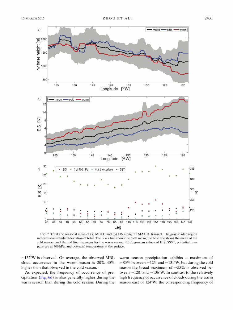
FIG. 7. Total and seasonal mean of (a) MBLH and (b) EIS along the MAGIC transect. The gray shaded region

indicates one standard deviation of total. The black line shows the total mean, the blue line shows the mean of the

cold season, and the red line the mean for the warm season. (c) Leg-mean values of EIS, SSST, potential tem-

perature at 700 hPa, and potential temperature at the surface.

15 MARCH 2015 ZHOU ET AL . 2431

occurrence of precipitation decreases rapidly. This

might be attributed to the presence of thin clouds at this

region (average thickness of 180m east of 1248W com-

pared to 300m west of 1248W).

The mean cloud-base height (Hb; Fig. 6e) and mean

cloud-top height (Ht; Fig. 6f) of the lowest cloud layer

show little seasonal variability except for the regions east

of 1258W. Mean values of Hb increase gradually from

0.6kmnear the coast of California to 1kmnear 1358Wand

remain at around 1km farther west but exhibit increasing

fluctuations, reflecting the intermittent presence of small-

scaleCu clouds below the Sc. TheHt values are on average

230m greater than those of Hb and also exhibit fluctua-

tions west of 1358W. East of 1258W we found the most

noticeable difference inHb andHt between the warm and

cloud season. The lowerHb east of 1258Wduring thewarm

season might be attributed to the stronger coastal up-

welling that results in lower SST (Fig. 6g), while the higher

Ht east of 1258W during the cold season might be attrib-

uted to a frontal system that occurred during Leg06B and

a low pressure system during Leg07B.

Most of the precipitation produced by MBL clouds is

in the form of virga (Fig. 6h). Virga is the dominant

precipitation type over the entire transect except for the

region east of 1268W. The virga frequency of occurrence

peaks at 40% near 1308W, whereas that of drizzle

(precipitation that reaches the lowest range gate) ex-

hibits a sharp maximum of more than 30% near 1248W,

contributing to the noticeable peak of precipitation

frequency at this location (Figs. 6b,d). The increasing

frequency of occurrence virga and decreasing frequency

of occurrence of drizzle from 1248 to 1308W (Fig. 6h)

might be attributed to the increasing cloud-base height

(Fig. 6e) caused by the warmer SST (Fig. 6g) away from

the California coast. The low frequencies of occurrence

(less than 10%) of both virga and drizzle near Hawaii

are consistent with the low frequency of occurrence of

MBL clouds there (Figs. 6a–c). At the same time, the

low frequencies of occurrence of both virga and drizzle

east of 1248W is associated with the presence of thinner

clouds in that region (Figs. 6e,f) and to the higher

in-cloud cloud droplet concentrations. Themean surface

CCN at 1198N is on average 150 cm3 higher than that

around 1228W (Lohmann and Feichter 2005).

2) SPATIAL AND SEASONAL BEHAVIOR OF MBLHAND EIS

The mean and seasonal values of MBLH and EIS

[Eq. (4)] along the MAGIC transect are shown in Fig. 7.

The mean MBLH (Fig. 7a) generally increases from Cal-

ifornia to Hawaii, with slightly lower values in the warm

season. The largest differences in MBLHs between the

warm season and cold season are observed east of 1258W,

with those observed during the cold season being nearly

twice as high as those during the warm season near the

coast of California. The low MBLH east of 1258W during

the warm season results in thin clouds [see section 4a(1)]

and correspondingly a low frequency of precipitation there

(Fig. 6d). The deeper MBL during the cold season is

consistent with the highHt (Fig. 6f), whichmight be due to

synoptic influences [see section 4a(1)]. The decrease in

MBLH between 1458 and 1508W can also be attributed to

synoptic influences and is discussed below. The trend in

MBLHalong theMAGIC transect (Fig. 7a) follows that of

Ht (Fig. 6f) east of 1358W, indicating the capped feature of

the MBL, while values of Ht west of 1358W are generally

less than those of MBLH, indicatingMBL decoupling and

Cu-under-Sc cloud regimes.

FIG. 8. Frequencies of occurrence of cloud types (a) over the entire deployment and (b) during

the cold season and warm season.

2432 JOURNAL OF CL IMATE VOLUME 28

The mean EIS (Fig. 7b) decreases gradually from 9K

near the coast of California to around 2K near Hawaii,

with values in the warm season being 1–3K higher and

those during the cold season 1–3K lower, the differences

decreasing toward Hawaii. EIS shows a strong linear re-

lationship with SST along the transect (figure not shown),

while in terms of the seasonal variability, leg-mean EIS

is mainly determined by the leg-mean potential tem-

perature at 700 hPa (Fig. 7c). This quantity exhibits

a larger seasonal variability, ranging from 7 to 11K

among different legs due to the subsidence of the dry

warm air from above the inversion layer, while usurface,

which depends largely on SST, varies less than 1K

between seasons.

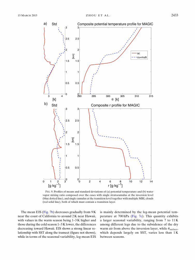
FIG. 9. Profiles of means and standard deviations of (a) potential temperature and (b) water

vapor mixing ratio composed over the cases with single stratocumulus at the inversion level

(blue dotted line), and single cumulus at the transition level together withmultipleMBL clouds

(red solid line), both of which must contain a transition layer.

15 MARCH 2015 ZHOU ET AL . 2433

It is likely that the seasonal variability of EIS (Fig. 7b)

contributes to the seasonal variability in the frequency

of occurrence of MBL clouds (higher amount of MBL

cloud in the warm season and lower in the cold season),

consistent with the conclusion of Wood and Bretherton

(2006) that stratus cloud fraction is largely determined

by EIS. The higher frequency of occurrence of MBL

clouds during the warm season when EIS was higher

(Fig. 6c) reflects the importance of the strong warm-

season large-scale Hadley cell (Xu and Cheng 2013) that

brings dry warm air downward, leading to higher values

of u700 (Fig. 7c).

3) SC AND CU OCCURRENCE AND

THERMODYNAMIC FEATURES

Frequencies of occurrence of the two important MBL

cloud types, Sc and Cu, are examined in this section.

Statistics of total and seasonal occurrence of Sc and Cu

are shown in Fig. 8. The frequency of occurrence of Sc

attains a broad maximum near 60% between 1258 and1358W, and decreases to near 0% near Hawaii. The

decrease in frequency of occurrence of Sc is not uniform

along the MAGIC transect, and is greatest near 1378Wand near 1448W, consistent with the sharp decreases in

MBL cloud occurrence (Fig. 6a) at these locations. In

contrast, the frequency of occurrence of Cu is always

low, but steadily increases from near 5% near the coast

of California to over 10% near Hawaii. Sc are more

frequently observed during the warm season than during

the cold season, while the occurrence of Cu is almost the

same for both seasons, with slightly more frequent cold-

season Cu close to the coast of California and slightly

more warm-season Cu close to Hawaii.

The comparison between ceilometer-detected Sc base

height and MBLH from 143 corresponding radiosondes

indicate that 80% of the Sc clouds formed directly below

the MBL inversion. Accordingly ceilometer-detected

Cu bases heights show broader distribution but mainly

occur near the top of the transition layer detected in 74

corresponding radiosondes (figures not shown). Figure 9

shows the averaged thermodynamic structure for Cu

(including multilayerMBL cloud) and single-layer Sc. A

total of 141 radiosondes were analyzed: 104 with Sc near

the inversion (Sc top no more than 200m below the

MBLH) and 37 with Cu near the transition or multilayer

cases (Cu base more than 200m above the transition-

layer tops). Application of a layer-by-layer averaging

method for the soundings for each cloud category (see

section 3d for details) requires detectable inversion and

transition layers. Analyses of theMAGIC sounding data

indicate that both layers are present in the vast majority

(94%) of the soundings. Note that the presence of

a transition layer does not necessarily indicate a sys-

tematic decoupled MBL (see section 3e).

As seen in Fig. 9, the large vertical gradients in po-

tential temperature and water vapor mixing ratio near

1.5 km indicate the heights and strengths of the inversion

layers, while the smaller changes below 1km correspond

to transition layers (Fig. 9). The standard deviations of

both potential temperature and mixing ratio for both

categories are relatively small below the inversion layer,

indicating little seasonal variability in profiles of these

quantities. Sc cases exhibit lower inversion- and

transition-layer heights than Cu cases, and they have

greater potential temperature differences across the in-

version (around 10K compared to near 5K for Cu); the

mixing ratio differences across the inversion are nearly the

same for both cases, around 6gkg21. Sc cases exhibit

smaller jumps across the transition layer than Cu for both

potential temperature (,0.5K compared to near 1K for

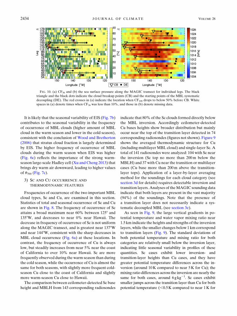
FIG. 10. (a) CF36 and (b) the sea surface pressure along the MAGIC transect for individual legs. The black

triangle and the black dots indicate the cloud breakup points (CB) and the starting points of the MBL systematic

decoupling (DE). The red crosses in (a) indicate the location when CF108 drops to below 50% before CB. White

spaces in (a) denote times when CF36 was less than 10%, and those in (b) denote missing data.

2434 JOURNAL OF CL IMATE VOLUME 28

Cu) and mixing ratio (,1gkg21 compared to 2gkg21 for

Cu); thus Cu cases are associated with a much stronger

transition layer than Sc, implying a greater chance of

a decoupled MBL. However, this stronger transition re-

sults in part because the cumuli help maintain the transi-

tion layer by mixing dry and warm air from the free

troposphere downward.

b. MBL systematic decoupling and cloud breakup

The locations of DE and CB for each leg are shown in

Fig. 10. Consistent with previous studies (e.g., Albrecht

et al. 1995a; Bretherton and Pincus 1995; Wyant et al.

1997; Sandu and Stevens 2011), DE occurred east of CB

(when the latter was determined) on all legs. In this

section, legs with both DE and CB detected are further

examined with the intention of discussing some of the

potential controlling factors that are usually neglected in

the numerical simulations.

1) POSSIBLE CONTROLLING FACTORS OF MBLSYSTEMATIC DECOUPLING

Since DEs and CBs occurred at different locations for

individual transects, a normalization of each leg is re-

quired in order to develop composites of variables

across these points. Each leg is divided into three re-

gions: east of DE, between DE and CB, and west of CB,

and the distance along the transect in each region is

normalized (i.e., for each leg, the distance from Cal-

ifornia to any location east of DE is divided by the dis-

tance between California and CB, and similarly for the

region between DE and CB, and CB and Hawaii).

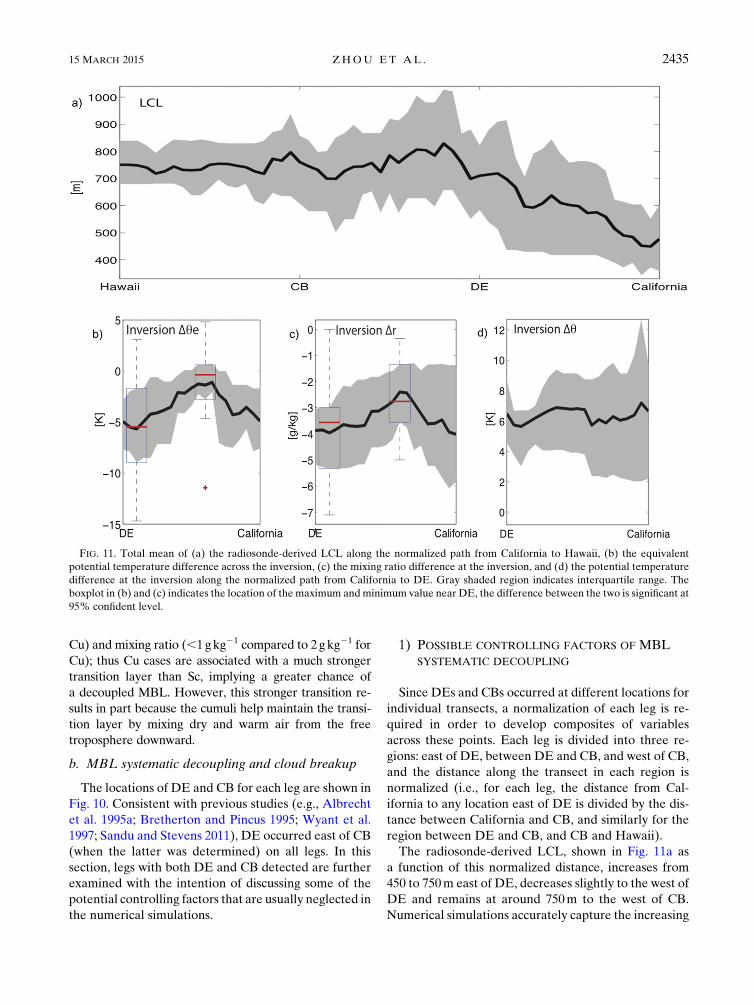
The radiosonde-derived LCL, shown in Fig. 11a as

a function of this normalized distance, increases from

450 to 750m east of DE, decreases slightly to the west of

DE and remains at around 750m to the west of CB.

Numerical simulations accurately capture the increasing

FIG. 11. Total mean of (a) the radiosonde-derived LCL along the normalized path from California to Hawaii, (b) the equivalent

potential temperature difference across the inversion, (c) the mixing ratio difference at the inversion, and (d) the potential temperature

difference at the inversion along the normalized path from California to DE. Gray shaded region indicates interquartile range. The

boxplot in (b) and (c) indicates the location of the maximum and minimum value near DE, the difference between the two is significant at

95% confident level.

15 MARCH 2015 ZHOU ET AL . 2435

trend of LCL with increasing SST over the well-mixed

MBL (Wyant et al. 1997; Sandu and Stevens 2011).

The LCL height is more sensitive to the surface

moisture than to the temperature. Thus, the increas-

ing LCL height implies a gradual drying of the MBL,

mainly due to the increasing entrainment rate with

higher SST that is necessary to maintain the energy

balance (Bretherton and Wyant 1997). During MAGIC,

it is found that the LCL increase rapidly near DE

(Fig. 11a), and the maximum increase in LCL with SST

near DEs ranges from 122 to 369mK21. The MAGIC

observations suggest that this sudden dryness of the

MBL is correlated with the entrainment of dryness

above the inversion.

Figure 11b shows the mean Due (i.e., averaged over

legs) over normalized distance from California to DE.

The value ofDue initially increased to near22K and then

decreased to26K at DE. This decrease is mainly due to

the large mean mixing ratio difference across the in-

version (Fig. 11c). Plausible explanations for the drier

conditions above the inversion are small displacements of

the Hadley cell or cold outbreaks behind trailing cold

fronts of midlatitude cyclones indicated by the increasing

sea surface pressure from California to DE (Fig. 10b).

The advection due to the large-scale circulation might

also contribute. Meanwhile, the increase in both the

potential temperature above the inversion (caused by

the subsidence of the dry warm air) and that below

(due to the increasing SST; Fig. 6g) explains the

maintenance of the mean potential temperature dif-

ference across the inversion of near 6K (Fig. 11d),

which contributed less to the decrease Due. The drop in

Due east of the DE point increases (Fig. 12) the cloud-

top entrainment instability and the entrainment rate

(Deardorff 1980) and subsequently less moisture in the

MBL. Consistent with the ‘‘deepening-warming mech-

anism’’ (Bretherton and Wyant 1997), our analysis

concurs that entrainment plays a crucial role in inducing

the MBL decoupling and the MAGIC observations also

suggest that the dry warm air above the inversion might

be an important trigger.

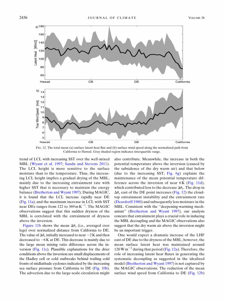
One would expect a dramatic increase of the LHF

east of DE due to the dryness of theMBL; however, the

mean surface latent heat was maintained around

120Wm22 during that period (Fig. 12a). Therefore, the

role of increasing latent heat fluxes in generating the

systematic decoupling as suggested in the idealized

model (Bretherton and Wyant 1997) is not captured by

the MAGIC observations. The reduction of the mean

surface wind speed from California to DE (Fig. 12b)

FIG. 12. The total mean (a) surface latent heat flux and (b) surface wind speed along the normalized path from

California to Hawaii. Gray shaded region indicates interquartile range.

2436 JOURNAL OF CL IMATE VOLUME 28

regulates the increase of the LHF, when the ship moves

from the edge to the center of the high pressure system

(Fig. 10b). Thus, we conclude that LHF might be im-

portant in maintaining the systematic decoupling, but

LHF does not play the dominant role in inducing de-

coupling in MAGIC, which is consistent with the con-

clusion of Jones et al. (2011).

Apart from the systematic decoupling, the weak de-

coupling (Dzi . 150m) east of DE is also investigated.

Broad peaks of the frequency of occurrence of virga and

drizzle were found east of DE, while these frequencies

decreased to below 20% when MBL was decoupled (fig-

ures not shown). We found that 87% of these are associ-

ated with precipitation. We conclude that precipitation

might play a role in inducing decoupling, but this decou-

pling is usuallyweak andnot continuous; thus, precipitation

did not show a dominant impact on systematic decoupling.

Meanwhile, diurnal decoupling might also partly explain

the weak decoupling east of DE since 73%of this occurred

in the local daytime from 6:00 a.m. to 6:00 p.m.

2) POSSIBLE CONTROLLING FACTORS OF MBLCLOUD BREAKUP DURING MAGIC

Values of CF36 are typically high along the eastern

part of theMAGIC transect (Fig. 10a), especially during

the warm season (Fig. 6). The locations where CF108

drop to below 50% are usually close to CB (CF108 drops

to below 15%), indicating the abrupt MBL cloud

breakup (Fig. 10a) At the same time, CB is typically

located on the west edge of high pressure systems

(Fig. 10b), implying the role of synoptic interference in

the observed MBL cloud breakup.

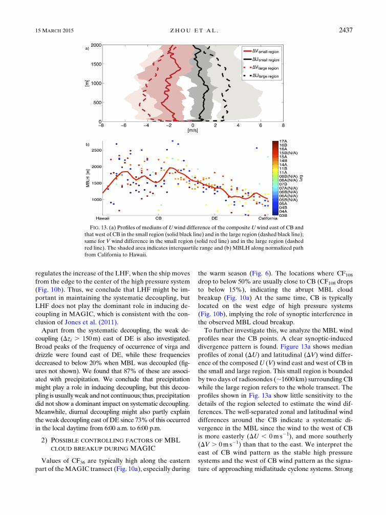
To further investigate this, we analyze the MBL wind

profiles near the CB points. A clear synoptic-induced

divergence pattern is found. Figure 13a shows median

profiles of zonal (DU) and latitudinal (DV) wind differ-

ence of the composedU (V) wind east and west of CB in

the small and large region. This small region is bounded

by two days of radiosondes (;1600km) surrounding CB

while the large region refers to the whole transect. The

profiles shown in Fig. 13a show little sensitivity to the

details of the region selected to estimate the wind dif-

ferences. The well-separated zonal and latitudinal wind

differences around the CB indicate a systematic di-

vergence in the MBL since the wind to the west of CB

is more easterly (DU , 0m s21), and more southerly

(DV . 0m s21) than that to the east. We interpret the

east of CB wind pattern as the stable high pressure

systems and the west of CB wind pattern as the signa-

ture of approaching midlatitude cyclone systems. Strong

FIG. 13. (a) Profiles of medians ofUwind difference of the compositeUwind east of CB and

that west of CB in the small region (solid black line) and in the large region (dashed black line);

same for V wind difference in the small region (solid red line) and in the large region (dashed

red line). The shaded area indicates interquartile range and (b) MBLH along normalized path

from California to Hawaii.

15 MARCH 2015 ZHOU ET AL . 2437

uplifting convergence in the east-approaching cyclones

was compensated by the divergence nearby. The drop of

the MBLH near CBs provides evidence of the com-

pensating subsidence (Fig. 13b), which is absent in the

idealized model with uniformed large-scale forcing.

Moreover, the averaged mixing ratio difference above

the inversion was nearly doubled in the small region

(not shown). We conclude that the switch of the syn-

optic environment to the unstable cyclone system can

rapidly break up the MBL cloud and drive vigorous

Cu or deep convective clouds.

5. Summary and discussion

The MAGIC field campaign, with nearly 200 days of

ship-based observations during 20 round trips along the

4000-km transect between California and Hawaii, pro-

vided an unparalleled opportunity to acquire data on

properties of MBL clouds, precipitation, and thermo-

dynamic structure. The measurements obtained during

that campaign are used in this manuscript to examine

the location and potential controlling factors of sys-

tematic MBL decoupling and Sc breakup.

MBL clouds were by far the most frequently observed

cloud type during the MAGIC campaign. MBL clouds

occurred more often during the warm season (Fig. 5),

reflecting the importance of the strong warm-season

large-scale Hadley cell (Xu and Cheng 2013). Among

the different MBL cloud types, Sc was the dominant

MBL cloud type and occurred more frequently during

the warm season than during the cold season (Fig. 8b),

while the occurrence of Cu was less strongly affected by

subsidence and exhibited nearly the same behavior for

both seasons (Fig. 8b).

The formation of Sc just below the inversion requires

a shallow MBL with a strong inversion and a weak tran-

sition (Fig. 9), providing a greater opportunity to have

well-mixed MBL conditions. In contrast, Cu and multi-

layer clouds are usually associated with a much stronger

transition, implying a greater chance of decoupling in

the MBL.

Therewas ahigh frequencyof occurrenceof precipitation

throughout the campaign. However, the precipitation from

the MBL clouds is weak and often evaporated well before

reaching the ocean surface (Fig. 6e). EIS experienced

a seasonal variation caused by that of u700 (Fig. 7c) and

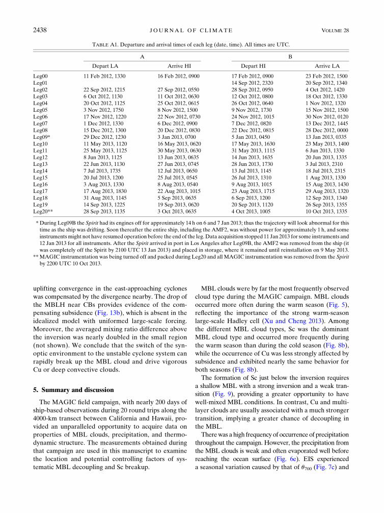
TABLE A1. Departure and arrival times of each leg (date, time). All times are UTC.

A B

Depart LA Arrive HI Depart HI Arrive LA

Leg00 11 Feb 2012, 1330 16 Feb 2012, 0900 17 Feb 2012, 0900 23 Feb 2012, 1500

Leg01 14 Sep 2012, 2320 20 Sep 2012, 1340

Leg02 22 Sep 2012, 1215 27 Sep 2012, 0550 28 Sep 2012, 0950 4 Oct 2012, 1420

Leg03 6 Oct 2012, 1130 11 Oct 2012, 0630 12 Oct 2012, 0800 18 Oct 2012, 1330

Leg04 20 Oct 2012, 1125 25 Oct 2012, 0615 26 Oct 2012, 0640 1 Nov 2012, 1320

Leg05 3 Nov 2012, 1750 8 Nov 2012, 1500 9 Nov 2012, 1730 15 Nov 2012, 1500

Leg06 17 Nov 2012, 1220 22 Nov 2012, 0730 24 Nov 2012, 1015 30 Nov 2012, 0120

Leg07 1 Dec 2012, 1330 6 Dec 2012, 0900 7 Dec 2012, 0820 13 Dec 2012, 1445

Leg08 15 Dec 2012, 1300 20 Dec 2012, 0830 22 Dec 2012, 0815 28 Dec 2012, 0000

Leg09* 29 Dec 2012, 1230 3 Jan 2013, 0700 5 Jan 2013, 0450 13 Jan 2013, 0335

Leg10 11 May 2013, 1120 16 May 2013, 0620 17 May 2013, 1630 23 May 2013, 1400

Leg11 25 May 2013, 1125 30 May 2013, 0630 31 May 2013, 1115 6 Jun 2013, 1330

Leg12 8 Jun 2013, 1125 13 Jun 2013, 0635 14 Jun 2013, 1635 20 Jun 2013, 1335

Leg13 22 Jun 2013, 1130 27 Jun 2013, 0745 28 Jun 2013, 1730 3 Jul 2013, 2310

Leg14 7 Jul 2013, 1735 12 Jul 2013, 0650 13 Jul 2013, 1145 18 Jul 2013, 2315

Leg15 20 Jul 2013, 1200 25 Jul 2013, 0545 26 Jul 2013, 1310 1 Aug 2013, 1330

Leg16 3 Aug 2013, 1330 8 Aug 2013, 0540 9 Aug 2013, 1015 15 Aug 2013, 1430

Leg17 17 Aug 2013, 1830 22 Aug 2013, 1015 23 Aug 2013, 1715 29 Aug 2013, 1320

Leg18 31 Aug 2013, 1145 5 Sep 2013, 0635 6 Sep 2013, 1200 12 Sep 2013, 1340

Leg19 14 Sep 2013, 1225 19 Sep 2013, 0620 20 Sep 2013, 1120 26 Sep 2013, 1355

Leg20** 28 Sep 2013, 1135 3 Oct 2013, 0635 4 Oct 2013, 1005 10 Oct 2013, 1335

*During Leg09B the Spirit had its engines off for approximately 14 h on 6 and 7 Jan 2013; thus the trajectory will look abnormal for this

time as the ship was drifting. Soon thereafter the entire ship, including the AMF2, was without power for approximately 1 h, and some

instrumentsmight not have resumed operation before the end of the leg.Data acquisition stopped 11 Jan 2013 for some instruments and

12 Jan 2013 for all instruments. After the Spirit arrived in port in Los Angeles after Leg09B, the AMF2 was removed from the ship (it

was completely off the Spirit by 2100 UTC 13 Jan 2013) and placed in storage, where it remained until reinstallation on 9 May 2013.

**MAGIC instrumentation was being turned off and packed during Leg20 and all MAGIC instrumentation was removed from the Spirit

by 2200 UTC 10 Oct 2013.

2438 JOURNAL OF CL IMATE VOLUME 28

generally decreased due to the increasing SST. MBLH

generally increased along the transect from California

to Hawaii (Fig. 7). East of 1358W the spatial behavior

of MBLH parallels that of the first cloud-top height

(Figs. 5f and 6d), indicating the capped feature of

the MBL.

The locations of MBL systematic decoupling are

determined for individual legs. It is found that

a threshold of Dq. 1.5 g kg21 separates the well-mixed

profiles from the systematic decoupled ones (Fig. 5b).

Compared to the threshold of Dq. 0.5 g kg21 found in

VOCAL-REx (Jones et al. 2011), the MAGIC sys-

tematic decoupling showed much stronger moisture

stratification below the inversion. Precipitation and

diurnal circulation correlate well with the weak de-

coupling points between California and DEs, but nei-

ther of them plays a dominant role in the systematic

decoupling.

A rapid increase of LCL height was found near DEs

(Fig. 11a), indicating more rapid drying of the MBL.

Correspondingly, the mean cloud-top instability showed

a sudden increase, mainly due to the large mixing ratio

difference across the inversion (Figs. 11b,c). These ob-

servations imply that the dry warm air from above the

inversion is likely of great importance triggering the

systematic decoupling. Consistent with the results in

VOCAL-REx (Jones et al. 2011), LHF does not play the

dominant role in inducing systematic decoupling in

MAGIC. Meanwhile, the mixed layer cloud thickness

duringMAGIC did not correlate well with the systematic

decoupling due to the sudden change of LCL near DEs,

further implying that the strong entrainment was driven

more by the cloud-top instability than by the in-cloud

turbulence.

DEs nearly always occurred east of CBs (if present)

(Fig. 10). MBL clouds tend to break up abruptly at

a location that is typically on the west edge of high

pressure systems (Fig. 10b). A change in synoptic pat-

tern (i.e., different air mass) was often found near CB,

which is associated with systematic divergence in the

MBL. The divergence, together with downdrafts, com-

pensated for the convergent uplifting in the approaching

cyclones. We conclude that the cloud evolution in the

idealized model seldom occurs in reality due to synoptic

interference.

Acknowledgments. The MAGIC deployment was

supported and undertaken by the U.S. Department of

Energy (DOE) Atmospheric Radiation Measure-

ment (ARM) Program Climate Research Facility. The

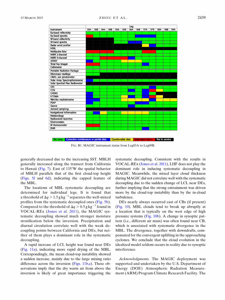
FIG. B1. MAGIC instrument status from Leg03A to Leg09B.

15 MARCH 2015 ZHOU ET AL . 2439

current research was supported by the DOE Atmo-

spheric System Research (ASR) Program (Office of

Science, OBER). ERL was supported by the ASR

Program under Contract DE-AC02-98CH10886. Data

used for the analyses were downloaded from the

ARM archive (www.arm.gov) except for the MARMET

and MARFLUX data, which were provided by

Dr. Michael Reynolds of RMR Co. We thank David

Painemal of NASA Langley Research Center for

providing surface cloud condensation nuclei (CCN)

data. We acknowledge the team of scientists and

technicians who made this work possible by collecting

the data and maintaining the instruments, and espe-

cially Horizon Lines and the captain and crew of the

Horizon Spirit for their hospitality. Special thanks go

to the cloud research group at McGill University

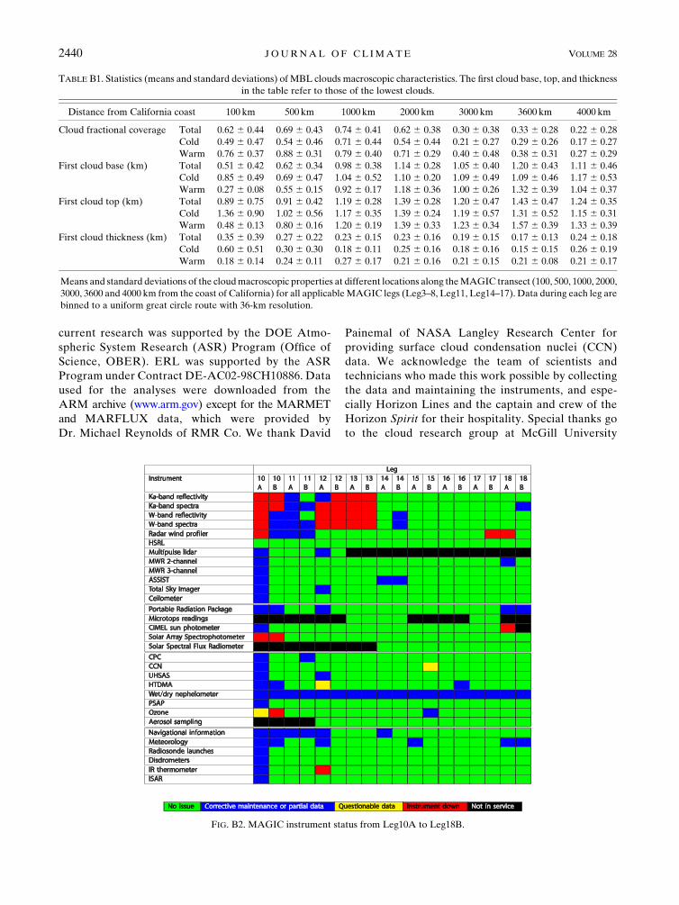
TABLE B1. Statistics (means and standard deviations) of MBL clouds macroscopic characteristics. The first cloud base, top, and thickness

in the table refer to those of the lowest clouds.

Distance from California coast 100 km 500 km 1000 km 2000 km 3000 km 3600 km 4000 km

Cloud fractional coverage Total 0.62 6 0.44 0.69 6 0.43 0.74 6 0.41 0.62 6 0.38 0.30 6 0.38 0.33 6 0.28 0.22 6 0.28

Cold 0.49 6 0.47 0.54 6 0.46 0.71 6 0.44 0.54 6 0.44 0.21 6 0.27 0.29 6 0.26 0.17 6 0.27

Warm 0.76 6 0.37 0.88 6 0.31 0.79 6 0.40 0.71 6 0.29 0.40 6 0.48 0.38 6 0.31 0.27 6 0.29

First cloud base (km) Total 0.51 6 0.42 0.62 6 0.34 0.98 6 0.38 1.14 6 0.28 1.05 6 0.40 1.20 6 0.43 1.11 6 0.46

Cold 0.85 6 0.49 0.69 6 0.47 1.04 6 0.52 1.10 6 0.20 1.09 6 0.49 1.09 6 0.46 1.17 6 0.53

Warm 0.27 6 0.08 0.55 6 0.15 0.92 6 0.17 1.18 6 0.36 1.00 6 0.26 1.32 6 0.39 1.04 6 0.37

First cloud top (km) Total 0.89 6 0.75 0.91 6 0.42 1.19 6 0.28 1.39 6 0.28 1.20 6 0.47 1.43 6 0.47 1.24 6 0.35

Cold 1.36 6 0.90 1.02 6 0.56 1.17 6 0.35 1.39 6 0.24 1.19 6 0.57 1.31 6 0.52 1.15 6 0.31

Warm 0.48 6 0.13 0.80 6 0.16 1.20 6 0.19 1.39 6 0.33 1.23 6 0.34 1.57 6 0.39 1.33 6 0.39

First cloud thickness (km) Total 0.35 6 0.39 0.27 6 0.22 0.23 6 0.15 0.23 6 0.16 0.19 6 0.15 0.17 6 0.13 0.24 6 0.18

Cold 0.60 6 0.51 0.30 6 0.30 0.18 6 0.11 0.25 6 0.16 0.18 6 0.16 0.15 6 0.15 0.26 6 0.19

Warm 0.18 6 0.14 0.24 6 0.11 0.27 6 0.17 0.21 6 0.16 0.21 6 0.15 0.21 6 0.08 0.21 6 0.17

Means and standard deviations of the cloudmacroscopic properties at different locations along theMAGIC transect (100, 500, 1000, 2000,

3000, 3600 and 4000 km from the coast of California) for all applicableMAGIC legs (Leg3–8, Leg11, Leg14–17). Data during each leg are

binned to a uniform great circle route with 36-km resolution.

FIG. B2. MAGIC instrument status from Leg10A to Leg18B.

2440 JOURNAL OF CL IMATE VOLUME 28

(www.clouds.mcgill.ca) for their helpful comments

and constructive criticism.

APPENDIX A

MAGIC Campaign Schedule

Departure and arrival times of each leg are listed in

Table A1.

APPENDIX B

MAGIC Instrument Status

a. Instrument status table Leg03A to Leg09B

The first leg with MAGIC instrumentation was

Leg01B during which the ISAR was installed. (MAGIC

instrument status from Leg03A to Leg09B is shown in

Figure B1, for cloud characteristic statistics see Table

B1). During Leg02A and Leg02B, for which instrument

status designations are not listed, the radars and other

instruments were being set up; some collected data during

these legs. During Leg03most of the instruments were up

and collecting data. On Leg09B, the instruments were

without power for extended times and were being shut

down. The instruments were removed from the ship after

Leg09B from January 2013 until May 2013.

b. Instrument status table Leg10A to Leg18B

MAGIC instruments were redeployed during

Leg10A, and the campaign continued until the end of

Leg20B. (MAGIC instrument status from Leg10A to

Leg18B is shown in Figure B2.) The technicians did not

report instrument status designations for Leg19A and

Leg19B, but these were probably similar to those for

Leg18B. During Leg20A and Leg20B the instruments

were being turned off, so few data were collected during

these legs (although sonde launches occurred on

Leg20A, meteorological data were collected until the

ship returned to port, and both radars were operating for

most of the two legs).

REFERENCES

Albrecht, B. A., 1984: A model study of downstream variations of

the thermodynamic structure of the trade winds. Tellus, 36A,

187–202, doi:10.1111/j.1600-0870.1984.tb00238.x.

——, D. A. Randall, and S. Nicholls, 1988: Observations of ma-

rine stratocumulus clouds during FIRE. Bull. Amer. Meteor.

Soc., 69, 618–626, doi:10.1175/1520-0477(1988)069,0618:

OOMSCD.2.0.CO;2.

——,C. S. Bretherton, D. Johnson,W.H. Scubert, andA. S. Frisch,

1995a: The Atlantic Stratocumulus Transition Experiment—

ASTEX. Bull. Amer. Meteor. Soc., 76, 889–904, doi:10.1175/

1520-0477(1995)076,0889:TASTE.2.0.CO;2.

——,M. P. Jensen, andW. J. Syrett, 1995b: Marine boundary layer

structure and fractional cloudiness. J. Geophys. Res., 100 (D7),

14 209–14 222, doi:10.1029/95JD00827.

Augstein, E., H. Schmidt, and F. Ostapoff, 1974: The vertical

structure of the atmospheric planetary boundary layer in un-

disturbed trade winds over the Atlantic Ocean. Bound.-Layer

Meteor., 6, 129–150, doi:10.1007/BF00232480.

Bohren, C., and B. Albrecht, 1998:Atmospheric Thermodynamics.

Oxford University Press, 402 pp.

Bretherton, C. S., and R. Pincus, 1995: Cloudiness and marine

boundary layer dynamics in the ASTEX Lagrangian experi-

ments. Part I: Synoptic setting and vertical structure. J. Atmos.

Sci., 52, 2707–2723, doi:10.1175/1520-0469(1995)052,2707:

CAMBLD.2.0.CO;2.

——, andM. C.Wyant, 1997: Moisture transport, lower-tropospheric

stability, and decoupling of cloud-topped boundary layers.

J.Atmos. Sci., 54, 148–167, doi:10.1175/1520-0469(1997)054,0148:

MTLTSA.2.0.CO;2.

Deardorff, J., 1980: Cloud top entrainment instability. J. Atmos.

Sci., 37, 131–147, doi:10.1175/1520-0469(1980)037,0131:

CTEI.2.0.CO;2.

Fairall, C. W., E. F. Bradley, D. P. Rogers, J. B. Edson, and G. S.

Young, 1996: Bulk parameterization of air–sea fluxes for Trop-

ical Ocean–Global Atmosphere Coupled Ocean–Atmosphere

Response Experiment. J. Geophys. Res., 101 (C2), 3747–3764,

doi:10.1029/95JC03205.

Heck, P.W., B. J. Byars, D. F. Young, P.Minnis, and E. F. Harrison,

1990: A climatology of satellite derived cloud properties over

marine stratocumulus regions. Preprints, Conf. on Cloud

Physics, San Francisco, CA, Amer. Meteor. Soc., J1–J7.

Hildebrand, P. H., and R. Sekhon, 1974: Objective determina-

tion of the noise level in Doppler spectra. J. Appl. Meteor.,

13, 808–811, doi:10.1175/1520-0450(1974)013,0808:

ODOTNL.2.0.CO;2.

Jones, C. R., C. S. Bretherton, and D. Leon, 2011: Coupled vs.

decoupled boundary layers in VOCALS-REx. Atmos. Chem.

Phys., 11, 7143–7153, doi:10.5194/acp-11-7143-2011.

Karlsson, J., G. Svensson, S. Cardoso, J. Teixeira, and S. Paradise,

2010: Subtropical cloud-regime transitions: Boundary layer

depth and cloud-top height evolution in models and observa-

tions. J. Appl. Meteor. Climatol., 49, 1845–1858, doi:10.1175/

2010JAMC2338.1.

Klein, S. A., andD. L. Hartmann, 1993: The seasonal cycle of low

stratiform clouds. J. Climate, 6, 1587–1606, doi:10.1175/

1520-0442(1993)006,1587:TSCOLS.2.0.CO;2.

Kollias, P., E. Clothiaux, M. Miller, B. Albrecht, G. Stephens, and

T. Ackerman, 2007:Millimeter-wavelength radars: New frontier

in atmospheric cloud and precipitation research. Bull. Amer.

Meteor. Soc., 88, 1608–1624, doi:10.1175/BAMS-88-10-1608.

Krueger, S. K., G. T. McLean, and Q. Fu, 1995: Numerical simu-

lation of the stratus-to-cumulus transition in the subtropical

marine boundary layer. Part I: Boundary-layer structure. J. At-

mos. Sci., 52, 2839–2850, doi:10.1175/1520-0469(1995)052,2839:

NSOTST.2.0.CO;2.

Lewis, E. R., and Coauthors, 2012: MAGIC: Marine ARM GPCI

Investigation of Clouds. DOE/SC-ARM-12-020, U.S. De-

partment of Energy, 12 pp.

Lilly, D. K., 1968: Models of cloud-topped mixed layers under

a strong inversion. Quart. J. Roy. Meteor. Soc., 94, 292–309,

doi:10.1002/qj.49709440106.

Lohmann, U., and J. Feichter, 2005: Global indirect aerosol ef-

fects: A review.Atmos. Chem. Phys., 5, 715–737, doi:10.5194/

acp-5-715-2005.

15 MARCH 2015 ZHOU ET AL . 2441

Matrosov, S. Y., 2007: Potential for attenuation-based estimations

of rainfall rate fromCloudSat.Geophys. Res. Lett., 34,L05817,

doi:10.1029/2006GL029161.

Moran, K. P., B. E. Martner, M. J. Post, R. A. Kropfli, D. C.

Welsh, and K. B. Widener, 1998: An unattended cloud-

profiling radar for use in climate research. Bull. Amer. Meteor.

Soc., 79, 443–455, doi:10.1175/1520-0477(1998)079,0443:

AUCPRF.2.0.CO;2.

Rémillard, J., P. Kollias, E. Luke, and R. Wood, 2012: Marine

boundary layer cloud observations in the Azores. J. Climate,

25, 7381–7398, doi:10.1175/JCLI-D-11-00610.1.

Sandu, I., and B. Stevens, 2011: On the factors modulating the

stratocumulus to cumulus transitions. J. Atmos. Sci., 68, 1865–

1881, doi:10.1175/2011JAS3614.1.

Teixeira, J., and Coauthors, 2011: Tropical and subtropical cloud

transitions in weather and climate prediction models: The

GCSS/WGNE Pacific Cross-Section Intercomparison (GPCI).

J. Climate, 24, 5223–5256, doi:10.1175/2011JCLI3672.1.

Tiedtke, M., W. A. Hackley, and J. Slingo, 1988: Tropical fore-

casting at ECMWF: The influence of physical parameteri-

zation on the mean structure of forecasts and analyses.

Quart. J. Roy. Meteor. Soc., 114, 639–664, doi:10.1002/

qj.49711448106.

Wang, S., B.A.Albrecht, and P.Minnis, 1993: A regional simulation

of marine boundary layer clouds. J. Atmos. Sci., 50, 4022–4043,

doi:10.1175/1520-0469(1993)050,4022:ARSOMB.2.0.CO;2.

Widener, K., N. Bharadwaj, and K. Johnson, 2012: Ka-band ARM

Zenith Radar (KAZR) instrument handbook. DOE Office of

Science Atmospheric RadiationMeasurement (ARM) Program,

19 pp.

Wood, R., 2012: Stratocumulus clouds.Mon. Wea. Rev., 140, 2373–

2423, doi:10.1175/MWR-D-11-00121.1.

——, and C. S. Bretherton, 2004: Boundary layer depth, entrain-

ment, and decoupling in the cloud-capped subtropical and

tropical marine boundary layer. J. Climate, 17, 3576–3588,

doi:10.1175/1520-0442(2004)017,3576:BLDEAD.2.0.CO;2.

——, and ——, 2006: On the relationship between stratiform low

cloud cover and lower-tropospheric stability. J. Climate, 19,

6425–6432, doi:10.1175/JCLI3988.1.

——,andCoauthors, 2011: TheVAMOSOcean–Cloud–Atmosphere–

Land Study Regional Experiment (VOCALS-REx): Goals,

platforms, and field operations.Atmos. Chem. Phys., 11, 627–

654, doi:10.5194/acp-11-627-2011.

Wyant,M.C., C. S. Bretherton, H.A. Rand, andD.E. Stevens, 1997:

Numerical simulations and a conceptual model of the sub-

tropical marine stratocumulus to trade cumulus transition.

J.Atmos. Sci., 54, 168–192, doi:10.1175/1520-0469(1997)054,0168:

NSAACM.2.0.CO;2.

Xu, K.-M., and A. Cheng, 2013: Evaluating low cloud simulation

from an upgradedmultiscalemodeling frameworkmodel. Part

I: Sensitivity to spatial resolution and climatology. J. Climate,

26, 5717–5740, doi:10.1175/JCLI-D-12-00200.1.

Yin, B., andB.A.Albrecht, 2000: Spatial variability of atmospheric

boundary layer structure over the eastern equatorial Pacific.

J. Climate, 13, 1574–1592, doi:10.1175/1520-0442(2000)013,1574:

SVOABL.2.0.CO;2.

2442 JOURNAL OF CL IMATE VOLUME 28