climate sensitive site index models for norway

Draft

Climate sensitive site index models for Norway

Journal: Canadian Journal of Forest Research

Manuscript ID cjfr-2015-0155.R3

Manuscript Type: Article

Date Submitted by the Author: 02-Feb-2016

Complete List of Authors: Antón-Fernández, Clara; Norwegian Institute of Bioeconomy Research Mola-Yudego, Blas; Norwegian Institute of Bioeconomy Research Dalsgaard, Lise; Norwegian Institute of Bioeconomy Research Astrup, Rasmus; Norwegian Institute of Bioeconomy Research

Keyword: climate change, Picea abies, Pinus sylvestris, boreal forest, productivity

https://mc06.manuscriptcentral.com/cjfr-pubs

Canadian Journal of Forest Research

Draft

1

Climate sensitive site index models for Norway

Clara Antón-Fernández, Blas Mola-Yudego, Lise Dalsgaard, and Rasmus

Astrup

1

Clara Antón-Fernández,1 Blas Mola-Yudego, Lise Dalsgaard, and Rasmus Astrup.Norwegian Institute of Bioeconomy Research

1Corresponding author (e-mail: [email protected]).

Can. J. For. Res. 99: 1–33 (2016) DOI: 10.1139/Zxx-xxx © 2016 NRC Canada

of 34



Draft

2 Can. J. For. Res. Vol. 99, 2016

Abstract: The present study aims to develop biologically sound and parsimonious2

site index models for Norway to predict changes in site index under different climatic3

conditions. The models are constructed using data from the Norwegian national4

forest inventory (NNFI) and climate data from the Norwegian meteorological5

institute. Site index was modeled using the potential modifier funtional form, with6

a potential component (POT) depending on site quality classes, and two modifier7

components (MOD): temperature, and moisture. Each of these modifiers was based8

on a portfolio of candidate variables. The best model for spruce dominated stands9

included temperature as modifier (R2 = 0.56). In the case of pine and deciduous10

dominated stands, the best models included both modifiers (R2 of 0.40 and 0.54,11

for temperature and moisture respectively). We illustrate the use of the models by12

analyzing the possible shift in SI for year 2100 under one (RCP4.5) of the benchmark13

scenarios adopted by the IPCC for its fifth Assessment Report. The models presented14

can be valuable for evaluating the effect of climate change scenarios in Norwegian15

forest.16

Key words: Climate change, Picea abies, Pinus sylvestris, Norway spruce, Scots pine,17

deciduous, boreal forest, productivity.18

©2016 NRC Canada

of 34



Draft

Antón-Fernández, Mola-Yudego, Dalsgaard, Astrup 3

1. Introduction19

Quantification and prediction of stand productivity is a key question in forest research,20

with evident implications in forest planning. The productivity of a given area has traditionally21

been estimated by measuring the height of dominant trees at a given age. This value, known22

as site index (SI), is assumed to be a valid surrogate for the potential productivity of a23

particular site. Site index is widely used as a measure of site quality as it can be estimated24

from direct measurements of height and age, and it is a good predictor of volume growth and25

yield (Weiskittel et al., 2011). Site index is also a prevalent key predictor in most traditional26

growth and yield models.27

The site index reflects inherent site characteristics, such as soil and climate, which are28

directly related to forest productivity. Except in the case of intensively managed stands (e.g.29

plantations subject to irrigation or fertilization) site index is generally assumed to remain30

constant through time (Assmann, 1970), as average soil and climatic variables have been31

assumed to remain stable. Therefore, many approaches oriented towards the estimation of site32

index include topographic or locational variables (e.g. slope, latitude, altitude) that relate to33

climate and soil conditions, providing good accuracy in the estimates.34

However, this static approach does no longer hold in the present context of future climatic35

changes, as it is reasonable to expect changes in site index in parallel to changes in climate36

conditions (e.g. Kauppi et al., 2014). This climatic uncertainty context urges for the devel-37

opment of adequate tools for a more dynamic estimation of site index. This is particularly38

relevant in high latitudes, where current climate change scenarios predict the largest tempera-39

ture increases (Stocker et al., 2013). In these regions, temperature is the main variable driving40

forest productivity, and therefore the expected changes will strongly affect forest productivity41

(Peltola et al., 2010).42

Climatic projections for Norway forecast a generally warmer and wetter climate (Stocker43

et al., 2013). The forecasted conditions for Norway are outside the range of conditions cur-44

rently present in Norway, particularly in the southernmost part. Hence, the importance of45

having a site index model that gives biologically sound estimates outside the range of ob-46

served conditions. Several empirical approaches for predicting SI from biophysical predictors,47

©2016 NRC Canada

of 34



Draft

4 Can. J. For. Res. Vol. 99, 2016

including climatic variables, have been developed. These approaches range from linear models48

(e.g., Nigh et al., 2004; Sharma et al., 2012) to nonparametric approaches (e.g., Sabatia and49

Burkhart, 2014; Weiskittel et al., 2011). Some nonparametric approaches seem to have gained50

some popularity, e.g. the random forest model (e.g., Crookston et al., 2010; Weiskittel et al.,51

2011), because of their high accuracy and lack of assumptions about how the independent52

variables relate to each other and the dependent variable. This approach has, however, an53

important drawback, that when used outside the range of the training data its predictions are54

unreliable (Sabatia and Burkhart, 2014). Linear regression models and similar approaches like55

generalized additive models, GAM, (e.g., Albert and Schmidt, 2010) or other semiparamet-56

ric additive smoothing approaches (e.g., Nothdurft et al., 2012) share, somehow, a similar57

drawback: since SI has biological constrains that are not directly considered within the linear58

model, linear models could predict unrealistic values when used outside the range of the fitting59

data.60

The present study aims to develop biologically sound and parsimonious models for pre-61

dicting changes in site index under different climatic conditions for the three main species in62

Norway. The models are constructed using data from the Norwegian national forest inventory63

and climate data from the Norwegian meteorological institute. We illustrate how the SI models64

can be used by estimating the SI shift in 2100 under one of the IPCC climate change scenarios.65

2. Material and methods66

2.1. Data sources67

The forest measurements for this study were based on data from the Norwegian National68

Forest Inventory (NNFI) measured during the period 2009-2013. The NNFI consists of perma-69

nent plots laid systematically on a 3x3 km grid, covering an extension from latitude 58.8N up70

to 70.8N. The grid covers the whole country except for the northernmost region (Finnmark).71

Plots with more than 20% of Sitka spruce (Picea sitchensis (Bong.) Carr.) were excluded, due72

to differences in measurement methods, and only plots located in productive forestland were73

considered, resulting in 8943 plots included in the calculations. The main species in Norway74

are, in this order, Norway spruce (Picea abies (L.) Karst.), Scots pine (Pinus sylvestris L.) and75

birch (Betula pendula Roth. and Betula pubecens Ehr.).76

©2016 NRC Canada

of 34



Draft


Site index (SI) was defined as the average height of the 100 thickest trees per hectare at77

the reference age of 40 years, and it is estimated at each cycle of the NNFI. At each plot78

the SI was assessed for the main species by selecting at least one dominant tree within a 0.179

ha circle. The selection of the dominant tree was done by visual assessment. The heights of80

the selected trees were measured and their corresponding ages were estimated from increment81

cores. The resulting data was used to estimate the SI according to Tveite and Braastad (1981),82

which places SI in classes: 6 (5-6.5), 8 (6.5-9.5), 11 (9.5-12.5), 14 (12.5-15.5), 17 (15.5-18.5),83

20 (18.55-21.5), 23(21.5-24.5), and 26 (>24.5) m.84

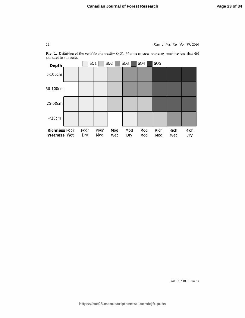
In addition, records of soil depth and understory vegetation class were taken at each plot.85

The understory vegetation classes were grouped into 9 categories (Astrup et al., 2010), accord-86

ing to their position along a gradient in nutrients (poor, moderate, and rich) and moisture87

(wet, moderate, and dry). The soil depth was classified in 4 categories: soil depth below 2588

cm, between 25 and 50 cm, between 50 and 100 cm, and above 100 cm. The resulting com-89

bination of soil richness, moisture, and depth form a total of 36 potential combinations, most90

of which are only represented by a small number of plots. These combinations were the basis91

of a categorical variable that organized richness, moisture and soil depth into five biologically92

meaningful groups. The groups were defined to minimize the SI variability for each species93

within each group. The new site quality variable (SQ) had a value of 1 to indicate the poorest94

sites and 5 to indicate the best sites (Figure 1).95

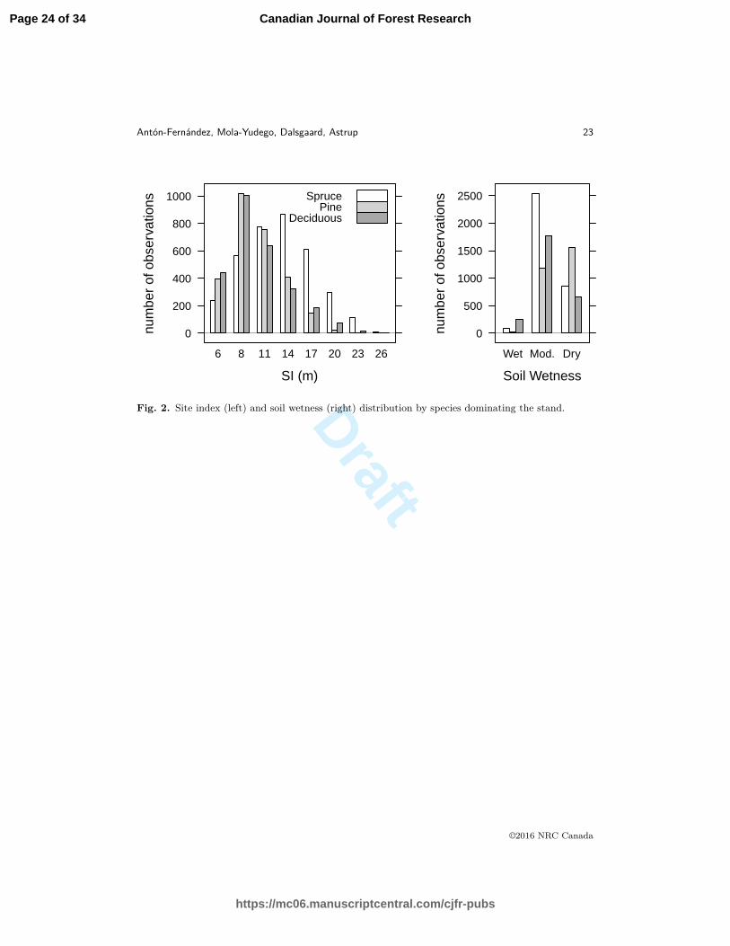
The location of spruce, pine and deciduous dominated stands in Norway is therefore re-96

flected in their frequency in each of the SQ groups defined (Table 1). Pine dominated stands97

are mostly located on poor sites (SQ1) while they are rare on the best sites (SQ5), whereas98

spruce dominated and deciduous dominated stands were mostly distributed in SQ3 and SQ4.99

The distribution of plots among SI classes is similar for deciduous and pine dominated stands100

(Figure 2). The lower SI classes are most commonly dominated by pine and deciduous species,101

while spruce dominated stands lead SI classes higher than 11m. The highest SI observed, 26m,102

is only found in few (12) spruce dominated stands. With respect to soil wetness, deciduous103

and spruce dominated stands are most common in moderate soils while pine are most common104

in dry soils (Figure 2). Most of the plots classified as wet are dominated by deciduous species,105

and only 18 of the plots classified as wet are dominated by pines.106

©2016 NRC Canada

of 34



Draft

6 Can. J. For. Res. Vol. 99, 2016

Historical climate data (1900-2008) at the plot level were provided by the Norwegian mete-107

orological institute. Monthly precipitation and temperature were geographically interpolated108

from about 400 weather stations throughout Norway. 30-years averages were calculated us-109

ing data from 1979-2008 (MET7908). We used the multimodel (67) ensemble mean monthly110

temperature and precipitation outcomes from representative concentration pathway (RCPs)111

4.5 (Thomson et al., 2011) from the CMIP5 21st century experiments (Royal Meterological112

Institute of The Netherlands (KNMI), 2014), RCP4.5, for projecting SI changes in 2100 for113

NNFI plots currently on forestland. RCP4.5 is one of the benchmark scenarios adopted by the114

IPCC for its fifth Assessment Report (Moss et al., 2008).115

2.2. Modeling approach116

Since the aim of this study is to predict changes in site index under changing climatic117

conditions it is important that the selected modeling approach produces models that behave118

well beyond the range of current climatic conditions. We use a multiplicative potential (POT)119

modifier (MOD) functional form for the SI model (SI = POT ×MOD) where MOD is scaled to120

only have values between 0 and 1. This functional form has the advantage of being constrained121

and robust since the predicted SI will not exceed the potential even when approaching the122

limits of the empirical data used for model development. In this modelling approach both123

the potential and modifiers are estimated as parameters in a nonlinear regression model. The124

applied modelling approach is equivalent to that frequently applied in studies of tree diameter125

growth where an estimated potential maximum growth rate (estimated as part of a nonlinear126

regression model) is modified according to site factors or competition for light or belowground127

resources (e.g. Lilles and Astrup, 2012; Canham and Uriarte, 2006). The approach applied in128

this analysis is different than the more conventional potential modifier approach (as in Belcher129

and Brand, 1982) where the potential is estimated in a separate analysis, and often using a130

different data set, than the one used for fitting the modifier. It is similar to the conventional131

potential modifier approach in the sense that the modifiers vary between 0 and 1 and modify132

how close to realization of the potential the estimated SI is.133

The SI was, therefore, modeled using the multiplicative potential modifier functional form.134

This functional form has two components: The potential component (POT), which can be135

©2016 NRC Canada

of 34



Draft


interpreted as the mean SI at a given SQ when neither temperature or moisture are limiting,136

and a modifier component (MOD) which reduces the potential site index according to relevant137

variables, in the form SI = POT × MOD. The modifier component can consist of one or138

several multiplicative modifiers, each of them taking values between 0 and 1, e.g. MOD =139

MOD1 · MOD2, which results in MOD varying between 0 and 1, and the model predicting140

values between 0 and POT . The potential modifier functional form is commonly used to model141

growth, where the lower limit of zero makes sense. However, when applied to SI modeling a142

value of zero does not make biological sense. Therefore, to account for a lower SI limit of 6,143

which is the minimum SI measured in the NNFI, we redefined the basic form of the model as:144

6 + (POT − 6) × MOD.145

The candidate modifiers included a temperature effect, MODT , and a moisture surplus146

effect MODM . For each modifier, a simple portfolio of candidate variables was considered.147

The modifier MODT included variables related to temperature that may affect SI, namely the148

number of growing days (GD, number of days with average temperature above 5◦C), and com-149

binations of the 30-year monthly average temperatures, for instance the temperature sum for150

spring and summer months (TSUM). The modifier MODM included variables related to water151

availability that may restrict the SI, and included several combinations of the 30-year monthly152

average precipitation, the Palmer drought severity index (Palmer, 1965), PDSI, for the grow-153

ing season months, the topographic wetness index (Beven and Kirkby, 1979), TWI, and the154

monthly moisture surplus defined as the difference between 30-year monthly average precipita-155

tion and the average monthly potential evapotranspiration (MSJ). We followed Thornthwaite156

(1948) to calculate potential evapotranspiration (PET) using the 30-year monthly average157

temperature:158

PET = 16K

(

10T

I

)m

I =12∑

i=1

(

T

5

)1.514

; m = 6.75 × 10−7I3− 7.71 × 10−5I2 + 1.79 × 10−2 + 0.492

©2016 NRC Canada

of 34



Draft

8 Can. J. For. Res. Vol. 99, 2016

K =(

N

12

)(

NDM

30

)

; N =(

24π

)

ωs

ωs = arccos (− tan φ tan δ) ; δ = 0.4093 sin(

2πJ

365− 1.405

)

159

Where T is the monthly-mean temperature (°C), I is a heat index, which is calculated as160

the sum of 12 monthly index values i, m is a coefficient depending on I, K is a correction161

coefficient computed as a function of the latitude and month, NDM is the number of days of162

the month, N is the maximum number of sun hours, ωs is the hourly angle of sun rising, φ is163

the latitude in radians, and δ is the solar declination in radians, J is the average Julian day of164

the month.165

The plots were grouped according to dominant species (spruce, pine, and deciduous plots)166

and equations were fit to each of these categories separately. All the candidate variables were167

preliminarily explored by examining graphically and analytically their explanatory power for168

site index, for each modifier and for each species. To explore the strength and shape of the169

relationship between site index and the candidate variables we fitted linear tail-restricted170

cubic splines (5 knots) functions to each candidate variable and species (Harrell, 2001). When171

analyzing the strenght of the association between site index and the candidate variables, cubic172

splines offer the advantage of allowing departures from the assumption of linearity in the173

association. In addition, correlation matrices were computed and examined, to determine the174

degree of intercorrelation among variables.175

The criteria for including the candidate variables in the final version of the models were:176

they had to be significant at the 0.05 level, and they had to provide the highest explanatory177

power of the candidate variables.178

Concerning the model shape of the modifiers, two basic forms were considered. Variables179

increasing with the value of the explanatory variable were modelled using the logistic functions180

1/ (1 + exp(−βX)), where X is a vector of explanatory variables, and β is the vector of param-181

eters to be estimated. Relationships reaching a peak at certain point and decreasing afterwards182

were modelled using the Weibull function γ/α · ((X − µ) /α)γ−1 exp (− ((X − µ) /α)γ), where183

X ≥ µ, and α>0, scaled to be bounded between 0 and 1. The Weibull function is a widely used184

©2016 NRC Canada

of 34



Draft


and flexible function that have a shape parameter (γ), a scale parameter(α), and a location185

parameter (µ). To bound the Weibull function between 0 and 1, we added a scaling factor186

(1/ξ) which multiplied the whole function and was calculated as the maximum value of the187

function, and we redefined X as188

X =

X

µ

X ≥ µ

otherwise.

Thus, (X − µ) will never be negative, and values of X below µ will result in the modifier189

taking a value of 0.190

The basic form of the model was 6+(POT − 6)×MOD, where MOD = MODT ×MODM ,191

resulting in two models, named md1 and md2. Model md1 includes the temperature modifier192

MODT , and model md2 includes both the temperature and the moisture availability modifier193

MODM .194

Finally, the models were assessed in order to identify which modifiers, and in which com-

bination, resulted in a better model. The assessment was based in the Akaike information

criterion, AIC, (Akaike, 1974), and BIC (Schwarz, 1978), and the proportion of variance ex-

plained by the model relative to that explained by the simple mean of the data, adjusted by

the sample size (n) and the number of regressors (p):

R2

adj = 1 −

(

n − 1n − p − 1

)

(

1 − R2)

R2 = 1 −

(

∑

i (yi − fi)2

∑

i (yi − y)2

)

where y is the mean of the observed SI, fi is the ith model predicted SI, and yi is the ith195

observed SI.196

To avoid, as much as possible, problems with convergence we used a simulated annealing197

algorithm (Goffe et al., 1994) implemented in the likelihood package (Murphy, 2015) in R198

(R Core Team, 2015) to fit all models. The likelihood package allows to find the maximum199

likelihood estimates of statistical models using simulated annealing, a global optimization200

©2016 NRC Canada

of 34



Draft

10 Can. J. For. Res. Vol. 99, 2016

algorithm, with or without bounded searches.201

2.3. Projections202

The temperature and precipitation outcomes from the multimodel ensemble for RCP4.5203

have a 0.5 degree spatial resolution. Since the source and resolution of these data are differ-204

ent from the ones used for fitting the models (MET7908), we estimated the 30-years monthly205

average temperature at each plot for the 2071-2100 period as the sum of MET7908 and the pro-206

jected change according to RCP4.5. We calculated the projected change according to RCP4.5207

as the difference between the average monthly temperature for the 1979-2008 period available208

from RCP4.5 and the 2071-2100 monthly average from RCP4.5. We used the estimates of the209

30-years monthly averages for the 2071-2100 period, calculated as the sum of MET7908 and210

the projected change according to RCP4.5, to calculate the variables required by the models,211

TSUM and MSJ.212

3. Results213

3.1. Model fitting214

Several candidate variables for MODT were available. The preliminary correlation matrices215

of the candidate variables showed that temperature and number of growing days were highly216

correlated and that the best temperature-based variable had higher correlation with SI than217

the number of growing days for all species. Among the best temperature variables there was218

little variation in their correlation with SI, and the correlation among them was high (>0.94).219

The graphical evaluation of the residuals of the linear tail-restricted cubic splines revealed220

that April, May, and June monthly temperatures performed best, but different months tended221

to perform better in different regions (e.g. northern region), while the sum of temperature in222

spring and early summer had a more consistent residual pattern. Therefore, we selected tem-223

perature in spring and early summer, defined as the sum of the 30-year average temperatures224

in April, May, and June (TSUM), for MODT . The range and distribution of these variables225

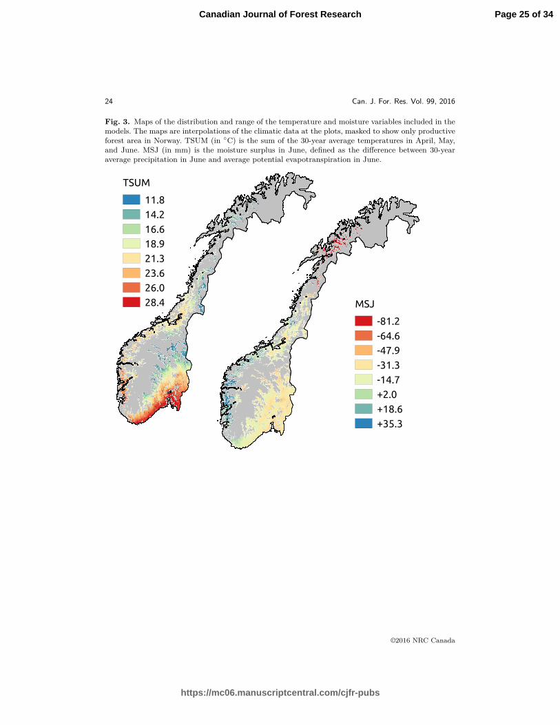
is shown in Figure 3.226

For MODM the correlations among candidate variables and SI were smaller than for227

MODT , but stronger for deciduous than for spruce or pine. Measures of goodness-of-fit (resid-228

©2016 NRC Canada

of 34



Draft


ual standard error and coefficient of determination R2) of the linear tail-restricted cubic splines229

revealed that water surplus in June outperformed all variables. Therefore, we selected moisture230

surplus in June (MSJ), defined as the difference between 30-year average precipitation in June231

and average potential evapotranspiration in June.232

The preliminary analysis determined the parameters that varied with SQ and the most233

adequate functional form for each modifier and for each species. We assessed graphically the234

need to make each parameter dependent on the SQ group. Table 2 shows the two modifiers235

selected for each species. In general, the variability explained by the best models, as measured236

by R2, was highest for spruce dominated plots, followed by deciduous and pine dominated237

plots. For all species the largest variability was explained by temperature.238

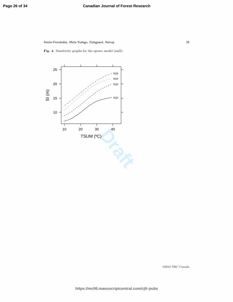
Consistently with the limiting factor theory, the sensitivity analyses revealed that the effect239

of temperature on SI was smaller for poorer sites and that this effect increases with site quality240

for all species (Figures 4, 5, and 6)241

In the spruce dominated stands, a large part of the variability was already explained by the242

model including TSUM (md1) in addition to the SQ factor (Table 3). In pine dominated stands243

(Table 3), model md2, with two modifiers, performed best. The full model (md2) improved AIC244

and R2 while keeping the estimates of the parameters within the expected range. A decrease245

in moisture surplus at the wetter sites results in an increase in SI, but once the optimum246

was reached, a drier climate (lower moisture surplus) results in a decrease in SI. The effect of247

temperature was greater at optimal moisture surplus, and it was very limited at the lowest248

and highest moisture surplus limits.249

Thus, we regarded md2 (temperature as modifier), md2 (temperature and moisture surplus250

as modifiers) and md2 (temperature and moisture surplus as modifiers) as the best models251

for spruce, pine and deciduous dominated stands, respectively. The selected models show little252

apparent trend in plots of residual values against either predicted values (Figure 7) or any of253

the indendent variables (data not shown).254

3.2. Projections255

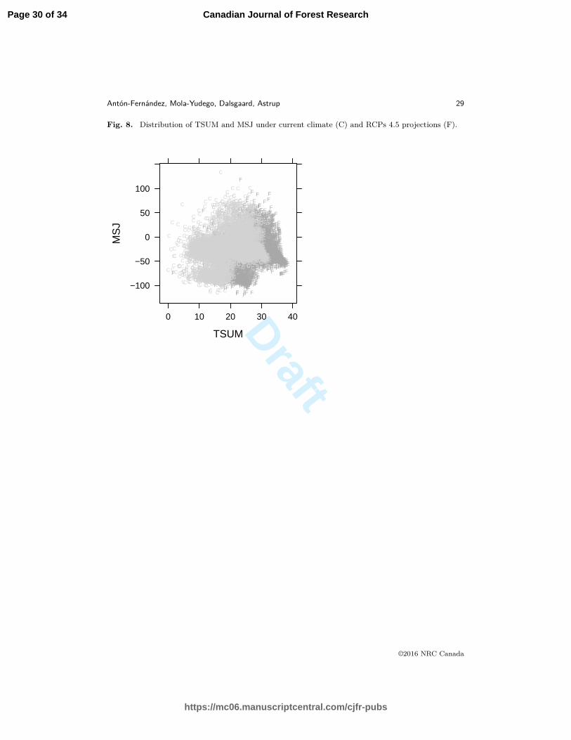
Climatic projections for Norway forecast a generally warmer and wetter climate, which256

results in a similar range of MSJ values, but a generally higher TSUM (Figure 8). Projections257

©2016 NRC Canada

of 34



Draft

12 Can. J. For. Res. Vol. 99, 2016

for SI in 2100 for the NNFI plots used for fitting the models were calculated by adding the258

expected change to the current SI. That is, we used the best models for each species to estimate259

SI for current conditions and for conditions in 2100, we then calculated the difference between260

these two and applied it to the current SI on each plot. For all species the patterns of SI remain261

similar to the current patterns of SI. The projections show that in most plots there will be an262

increase or no change in SI, with pine being the species less affected by climate change. The263

projections show constant or increasing SI, with very rare occurrences of decreasing SI (Figure264

9). The largest changes in SI are for spruce dominated stands, where the projections show an265

increase in SI of at least 1 meter in most regions, with a higher increase in the central part of266

Norway and plots close to the tree line in the southern part of Norway. For pine dominated267

stands the increase in SI was more moderate, with most of the plots experiencing little change.268

For deciduous dominated stands the change in SI was bellow 3 meters in most plots, with little269

change in the northernmost regions, and only few plots experiencing increases of SI above 3270

meters. The range of MSJ on the original data (-115, 134) does not differ much from the range271

of MSJ on RCP4.5 (-119, 118), being the average change in MSJ -6.5 mm. The average change272

in TSUM in RCP4.5 with respect to MET7908 was 6.5 ◦C. The range of TSUM change from273

(0, 32.5) in MET7908 to (1.6, 38.5) in RCP4.5.274

4. Discussion275

The present paper explains the variations of SI in Norway according to climatic and soil276

conditions by using an empirical approach. The models are fit using an extensive data pool277

resulting from the NNFI and environmental variables from the Norwegian meteorological insti-278

tute. Thus, an application to recent climate conditions becomes straightforward. At the same279

time, the models are biologically sound, and efficiently represent the main limitations to forest280

growth in Norwegian conditions.281

However, there are limitations in the data used for the estimation of the SI: in general,282

the overall estimation of site index based on a reference height is a difficult task subject283

to measurement error and the site classes in Norway are defined in intervals, which reduces284

the precision of the predictions. Despite these limitations, the NNFI is the largest data set285

available for the region and covers systematically a broad geographical region with diverse286

©2016 NRC Canada

of 34



Draft


climate conditions, thus providing a solid empirical basis for the models presented.287

The models presented precision levels similar to other recent studies of SI prediction using288

alternative statistical approaches (e.g. Seynave et al., 2005; Albert and Schmidt, 2010; Aertsen289

et al., 2010). In Norway, Sharma et al. (2012) presented SI models for Norway spruce and Scots290

pine with higher predictive power than the ones presented here. Sharma et al. (2012) used linear291

regression models and the year of stand establishment, the temperature sum (degree days above292

5ºC), location, topography, soil, and understory vegetation variables as explanatory variables.293

Although Sharma’s et al. R2 values may look promising (up to 0.85 for Norway spruce and294

0.72 for Scots pine), their models present several limitations when used for prognoses under295

climate change. They assume a linear relationship between temperature sum and SI, thus296

higher temperatures will always, regardless of precipitation, result in higher SI. The inclusion of297

the year of stand establishment results in a continuous trend of higher SI in newly established298

stands, which may result in illogical SI when used for prediction of long-term prognoses.299

Recent studies on SI prediction have focused on modeling the spatial SI trends. For example,300

Albert and Schmidt (2010) used generalized additive regression models with a two-dimensional301

location component to model the spatial SI trend. We chose not to include location components302

in our models because, in our case, location is correlated with the main variables of interest303

(the correlations between TSUM and latitude and longitude are 0.47, and 0.36 respectively,304

and between MMS and latitude and longitude are 0.47, and 0.72, respectively) and that would305

cause confounding of the effects of changes in the climatic variables. Other options to address306

spatial correlation is that of Nothdurft et al. (2012), who applied a simplified universal kriging307

method using B-spline basis functions to provide spatio-temporal predictions of site index308

for an area of Southwest Germany. The Nothdurft et al. (2012) approach requires that the309

mean function of the spatial site-index process, the one that depends on climatic variables, to310

be linear. Since the relationship between SI and most of the climatic variables is non-linear,311

the relationships are linearized through the B-spline functions. Nothdurft et al. (2012) chose312

the number and location of the B-spline knots heuristically to avoid illogical behavior when313

extrapolating beyond the range of the model data. The strength of the approach selected in the314

present paper is that we ensure biologically sound results beyond the current range of climatic315

conditions, and that behavior is defined by the data and the basic form of the models, avoiding316

©2016 NRC Canada

of 34



Draft

14 Can. J. For. Res. Vol. 99, 2016

having to select heuristically some of the parameters. Other interesting approach to model the317

effects of biophysical factors on tree growth is to model the effect of biophysical factors on the318

potential tree height as it is done in SILVA (Pretzsch et al., 2002). This approach, however,319

requires data on dominant height, which is neither currently recorded by the NNFI nor is320

available from experimental plots in a representative scale for Norwegian conditions.321

Our results show that SI increases with temperature. Due to interaction effects between322

temperature and site quality, the increase becomes more pronounced with increasing site qual-323

ity. This results are congruent with Sigurdsson et al. (2013), who found that the effect of324

increase on temperature or CO2 on mature Norway spruce in the boreal zone was not evident325

unless nutrient availability was improved. Our results are also consistent with Pretzsch et al.326

(2014) findings that growth acceleration, likely due to climate change, for Norway spruce since327

1960 in Central Europe is stronger in more fertile sites.328

The effects of the variables included in the final version of the models were logical and329

in line with previous studies. In Norway, Andreassen et al. (2006) underlined the effect of330

temperature and precipitation on Norway spruce growth based on tree-ring series. Andreassen331

et al. (2006) concluded that, of the variables explored, June temperature and precipitation332

had the largest influence on tree ring increments of the variables explored, which is consistent333

with our results. For all three species, most of the variability was explained by MODT , which334

is also consistent with previous studies on the relationship between climatic factors and tree335

growth in Fennoscandia, which show that growth is mainly determined by summer temperature336

(e.g. Ge et al., 2011; Andreassen et al., 2006). Ge et al. (2011) used a process-based growth337

model to assess the impacts of climate change on stem wood growth. They found that most of338

the variability of annual growth in Norway spruce in Finland was explained by temperature,339

particularly June temperature, while the relationship between annual growth and monthly340

precipitation was more subtle. Andreassen et al. (2006) also found stronger correlations of341

growth with summer temperatures than with monthly precipitation for Norway spruce in342

Norway. The fact that moisture surplus is not included in the final model for spruce is not343

to say that that moisture surplus is not an important factor in spruce dominated stands344

productivity. Rather, it indicates that moisture surplus is not a limiting factor within the345

current range of spruce dominated stands.346

©2016 NRC Canada

of 34



Draft


For pine dominated stands the optimal MSJ is lower than for deciduous dominated stands.347

This is not surprising, since pine dominated stands are already dominating the drier sites in348

Norway (Figure 2).349

One of our main objectives was to make the models biologically sound, which is a require-350

ment when the aim of the models is to forecast the productivity of large non-homogeneous351

areas. To achieve this objective we used empirical data and a modeling approach that bounds352

the response of the model between a maximum, the potential, and a minimum, defined as the353

minimum recorded SI (6m). As a result of this, even if the conditions on a plot for a certain354

species become unsuitable for the survival of the species or the plot becomes unproductive, the355

model will still give an estimate of the SI between the minimum and the maximum. Predict-356

ing the suitability of a site for the survival or establishment of a species should be answered357

separately, and it is not within the scope of this paper.358

There are other considerations that should be taken into account when applying climate359

sensitive SI models. One should be careful when applying these models to already established360

stands, as the climate-growth response of the stands already established might depend on361

the provenance of the trees, their age, and elevation, among other factors (Primicia et al.,362

2015). Productivity might also be affected by other factors that might change with time and363

that are not considered here, like CO2, nitrogen deposition (Sigurdsson et al., 2013), nutrient364

availability, and solar radiation.365

The potential component (POT) is the mean SI index at a given site quality (SQ) when366

neither temperature or moisture are limiting. Even under the best climatic conditions there367

are other factors that limit the growth of trees, such as light and nutrient availability, or me-368

chanical factors (e.g. wind, snow). Since the fit of a model is usually performed by minimizing369

weighted errors, the model will predict the average SI found under certain site conditions,370

temperature, and precipitation, which will never be the maximum SI observed because of the371

imperfect correlation between SI and the variables of the models, and the error implicit in372

the measurements of the variables. Thus, the models correctly predict trends due to a change373

in temperature or precipitation, but they will predict expected SI under given conditions. In374

order to predict future SI under climate change, we suggest that the models should be used375

to predict SI change (predicted SI in future climate - predicted SI in current climate) which376

©2016 NRC Canada

of 34



Draft

16 Can. J. For. Res. Vol. 99, 2016

then is added to the currently observed SI. If no information about the current site index is377

available, the models can be used directly but with an expectation of a larger error than when378

current site index information is available. If there is information about current SI and the379

model is used to predict SI change, the predicted SI can exceed POT.380

Thanks to the broad array of conditions currently present in Norway we have been able to381

use the space-for-time substitution, an approach widely used in other fields such as biodiversity382

modeling (Blois et al., 2013), to predict climate change effects on SI for Norway. The space-for-383

time substitution assumes that spatial and temporal variation are equivalent. This approach is384

commonly used accross fields when long-term time-series data are not available. However, this385

approach has some drawbacks that should be considered. For example, as with any empirical386

model, caution should be used when extrapolating beyond the original range. Also, although387

SI is assessed at each cycle of the NNFI, the observed SI is the result of the stand history and388

climate throughout the life of the trees currently in the stand, and as so, it is an imperfect389

measurement of the current SI if a new stand were to be established. Since the observed SI is390

the result of the compound response over the life span of the trees, we chose to use the average391

of the climatic variables over the last 30-years, instead of using only more recent data, as the392

explanatory variable for our SI models.393

When the best models are applied using climate projections for 2100 (RCP4.5), the patterns394

of change observed in Figure 9 reflect the behavior of the models. The general trend for all plots395

considered and all species is an increase in SI for 2100. For more extreme climate scenarios (e.g.396

RCP8.5) the results may be considerably different than under RCP4.5. The moisture indicator,397

MSJ, does not change dramatically between MET7908 and RCP4.5, which is why there are only398

very few plots with a decrease in SI greater than 1 meter (Figure 9). Contrary to the presented399

results, studies from other parts of the boreal forest indicate reduced forest productivity. For400

example, projections for Canada under climate change indicate a likely decrease in productivity401

in areas with relative high water stress and low water-holding capacity, but an increase on forest402

productivity on sites with high water-holding capacity during the 21st century (Johnston et al.,403

2009). In northern Finland, where soil moisture seldom limits forest growth, stem wood growth404

are expected to be higher under climate change, while in sourthern Finnland stem wood growth405

is, on average, lower under climate change due to limited water availability compared with the406

©2016 NRC Canada

of 34



Draft


current climate (Ge et al., 2011). Climatic projections for Norway forecast a generally warmer407

and wetter climate (Stocker et al., 2013), and at least for RCP4.5, it seems that the higher408

precipitation will, in general, compensate the higher water requirements and result in higher409

productivity for most areas in Norway and mainly for spruce and deciduous dominated stands.410

Finally, despite the restrictions of the modelling approach and the obvious limitations411

in forest growth prognoses, the models presented in this paper present a robust and easily412

applicable basis for SI prediction in boreal conditions.413

5. References414

References415

Aertsen, W., Kint, V., van Orshoven, J., Özkan, K., Muys, B., 2010. Comparison and ranking416

of different modelling techniques for prediction of site index in Mediterranean mountain417

forests. Ecological Modelling 221, 1119–1130.418

Akaike, H., 1974. A new look at the statistical model identification. IEEE transactions on419

automatic control 19, 716–723.420

Albert, M., Schmidt, M., 2010. Climate-sensitive modelling of site-productivity relationships421

for Norway spruce (Picea abies L. Karst.) and common beech (Fagus sylvatica L.). Forest422

Ecology and Management 259, 739–749.423

Andreassen, K., Solberg, S., Tveito, O.E., Lystad, S.L., 2006. Regional differences in climatic424

responses of Norway spruce (Picea Abies L. Karst) growth in Norway. Forest Ecology and425

Management 222, 211–221.426

Assmann, E., 1970. Principles of forest yield study. Pergamon Press Ltd., Oxford.427

Astrup, R., Dalsgaard, L., Eriksen, R., Hylen, G., 2010. Utviklingsscenarioer for karbonbind-428

ing i Norges skoger [Development scenarios for carbon sequestration in Norwegian forest].429

Oppdragsrapport fra Skog og landskap 16/10. Norwegian Forest and Landscape Institute.430

Ås, Norway. In Norwegian with English summary.431

Belcher, D.M., Brand, G.J., 1982. A description of STEMS- the stand and tree evaluation and432

modeling system. Gen. Tech. Rep.433

©2016 NRC Canada

of 34



Draft

18 Can. J. For. Res. Vol. 99, 2016

Beven, K.J., Kirkby, M.J., 1979. A physically based, variable contributing area model of basin434

hydrology. Hydrological Sciences Bulletin 24, 43–69.435

Blois, J.L., Williams, J.W., Fitzpatrick, M.C., Jackson, S.T., Ferrier, S., 2013. Space can436

substitute for time in predicting climate-change effects on biodiversity. Proc. Natl. Acad.437

Sci. U.S.A. 110, 9374–9379.438

Canham, C.D., Uriarte, M., 2006. Analysis of neighborhood dynamics of forest ecosystems439

using likelihood methods and modeling. Ecological Applications 16, 62–73.440

Crookston, N.L., Rehfeldt, G.E., Dixon, G.E., Weiskittel, A.R., 2010. Addressing climate441

change in the forest vegetation simulator to assess impacts on landscape forest dynamics.442

Forest Ecology and Management 260, 1198–1211.443

Ge, Z.M., Kellomäki, S., Peltola, H., Zhou, X., Wang, K.Y., Väisänen, H., 2011. Impacts of444

changing climate on the productivity of Norway spruce dominant stands with a mixture of445

Scots pine and birch in relation to water availability in southern and northern Finland. Tree446

Physiol. .447

Goffe, W.L., Ferrier, G.D., Rogers, J., 1994. Global optimization of statistical functions with448

simulated annealing. Journal of Econometrics 60, 65–99.449

Harrell, F.E., 2001. Regression modelling strategies with applications to linear models, logistic450

regression, and survival analysis. Springer, New York, NY.451

Johnston, M.H., Campagna, M., Gray, P.A., Kope, H.H., Loo, J.A., Ogden, A.E., O’Neill, G.,452

Price, D.T., Williamson, T.B., 2009. Vulnerability of Canada’s tree species to climate change453

and management options for adaptation: an overview for policy makers and practitioners.454

Res. Coun. Pub. 12416-1E10. Canadian Council of Forest Ministers.455

Kauppi, P.E., Posch, M., Pirinen, P., 2014. Large Impacts of Climatic Warming on Growth of456

Boreal Forests since 1960. PLoS ONE 9, e111340.457

Lilles, E.B., Astrup, R., 2012. Multiple resource limitation and ontogeny combined: a growth458

rate comparison of three co-occurring conifers. Can. J. For. Res. 42, 99–110.459

©2016 NRC Canada

of 34



Draft


Moss, R.H., Babiker, M., Brinkman, S., Calvo, E., Carter, T., Edmonds, J.A., Elgizouli, I.,460

Emori, S., Lin, E., Hibbard, K., others, 2008. Towards new scenarios for analysis of emis-461

sions, climate change, impacts, and response strategies. Technical Report. Pacific Northwest462

National Laboratory (PNNL), Richland, WA (US).463

Murphy, L., 2015. likelihood: Methods for maximum likelihood estimation, R package version464

1.7.465

Nigh, G., Ying, C.C., Qian, H., 2004. Climate and productivity of major conifer species in the466

interior of British Columbia, Canada. Forest Science 50, 659–671.467

Nothdurft, A., Wolf, T., Ringeler, A., Böhner, J., Saborowski, J., 2012. Spatio-temporal pre-468

diction of site index based on forest inventories and climate change scenarios. Forest Ecology469

and Management 279, 97–111.470

Palmer, W., 1965. Meteorological drought. Res. Pap. 45 45. U.S. Weather Bureau.471

Peltola, H., Ikonen, V.P., Gregow, H., Strandman, H., Kilpeläinen, A., Venäläinen, A., Kel-472

lomäki, S., 2010. Impacts of climate change on timber production and regional risks of473

wind-induced damage to forests in Finland. Forest Ecology and Management 260, 833–845.474

Pretzsch, H., Biber, P., Schütze, G., Uhl, E., Rötzer, T., 2014. Forest stand growth dynamics475

in Central Europe have accelerated since 1870. Nature Communications 5.476

Pretzsch, H., Biber, P., Ďurský, J., 2002. The single tree-based stand simulator SILVA: con-477

struction, application and evaluation. Forest Ecology and Management 162, 3–21.478

Primicia, I., Camarero, J.J., Janda, P., Čada, V., Morrissey, R.C., Trotsiuk, V., Bače, R.,479

Teodosiu, M., Svoboda, M., 2015. Age, competition, disturbance and elevation effects on480

tree and stand growth response of primary Picea abies forest to climate. Forest Ecology and481

Management 354, 77–86.482

R Core Team, 2015. R: A language and environment for statistical computing. R Foundation483

for Statistical Computing. Vienna, Austria.484

©2016 NRC Canada

of 34



Draft

20 Can. J. For. Res. Vol. 99, 2016

Royal Meterological Institute of The Netherlands (KNMI), 2014. CMIP5 Scenario Runs485

- Surface Variables [online]. http://climexp.knmi.nl/selectfield\_cmip5.cgi\?id=486

someone@somewhere. [accessed 14 jun 2014].487

Sabatia, C.O., Burkhart, H.E., 2014. Predicting site index of plantation loblolly pine from488

biophysical variables. Forest Ecology and Management 326, 142–156.489

Schwarz, G., 1978. Estimating the dimension of a model. Ann. Stat. 6, 461–464.490

Seynave, I., Gégout, J.C., Hervé, J.C., Dhôte, J.F., Drapier, J., Bruno, E., Dumé, G., 2005.491

Picea abies site index prediction by environmental factors and understorey vegetation: a492

two-scale approach based on survey databases. Canadian Journal of Forest Research 35,493

1669–1678.494

Sharma, R.P., Brunner, A., Eid, T., 2012. Site index prediction from site and climate variables495

for Norway spruce and Scots pine in Norway. Scandinavian Journal of Forest Research 27,496

619–636.497

Sigurdsson, B.D., Medhurst, J.L., Wallin, G., Eggertsson, O., Linder, S., 2013. Growth of498

mature boreal Norway spruce was not affected by elevated [CO2] and/or air temperature499

unless nutrient availability was improved. Tree Physiology 33, 1192–1205.500

Stocker, T.F., Qin, D., Plattner, G.K., Tignor, M., Allen, S.K., Boschung, J., Nauels, A., Xia,501

Y., Bex, V., Midgley, P.M. (Eds.), 2013. Climate change 2013: The physical science basis.502

Contribution of Working Group I to the Fifth Assessment Report of the Intergovernmental503

Panel on Climate Change. Cambridge University Press, Cambridge, United Kingdom and504

New York, NY, USA.505

Thomson, A.M., Calvin, K.V., Smith, S.J., Kyle, G.P., Volke, A., Patel, P., Delgado-Arias, S.,506

Bond-Lamberty, B., Wise, M.A., Clarke, L.E., Edmonds, J.A., 2011. RCP4.5: a pathway for507

stabilization of radiative forcing by 2100. Climatic Change 109, 77–94.508

Thornthwaite, C.W., 1948. An approach toward a rational classification of climate. Geograph-509

ical review 38, 55–94.510

Tveite, B., Braastad, H., 1981. Bonitering for gran, furu og bjork. Norsk Skogbruk 27, 17–22.511

©2016 NRC Canada

of 34



Draft


Weiskittel, A.R., Crookston, N.L., Radtke, P.J., 2011. Linking climate, gross primary produc-512

tivity, and site index across forests of the western United States. Canadian Journal of Forest513

Research 41, 1710–1721.514

©2016 NRC Canada

of 34



Draft

of 34



Draft


SI (m)

num

ber

of o

bser

vatio

ns

0

200

400

600

800

1000

6 8 11 14 17 20 23 26

SprucePine

Deciduous

Soil Wetness

num

ber

of o

bser

vatio

ns

0

500

1000

1500

2000

2500

Wet Mod. Dry

Fig. 2. Site index (left) and soil wetness (right) distribution by species dominating the stand.

©2016 NRC Canada

of 34



Draft

24 Can. J. For. Res. Vol. 99, 2016

Fig. 3. Maps of the distribution and range of the temperature and moisture variables included in themodels. The maps are interpolations of the climatic data at the plots, masked to show only productiveforest area in Norway. TSUM (in ◦C) is the sum of the 30-year average temperatures in April, May,and June. MSJ (in mm) is the moisture surplus in June, defined as the difference between 30-yearaverage precipitation in June and average potential evapotranspiration in June.

��

��

��

��

��

��

��

�

��

��

��

��

��

��

��

��

��

©2016 NRC Canada

of 34



Draft


Fig. 4. Sensitivity graphs for the spruce model (md2).

TSUM (ºC)

SI (

m)

10

15

20

25

10 20 30 40

SQ2

SQ3

SQ4

SQ5

©2016 NRC Canada

of 34



Draft

26 Can. J. For. Res. Vol. 99, 2016

Fig. 5. Contour plots showing the behavior of md2 for pine dominated stands. Grey rectanglesindicate combinations of MSJ, TSUM and SQ that existed in the fitting dataset.

TSUM (ºC)

MS

J (m

m)

−50

0

50

10 20 30

78

9

SQ1

7

89

1011

1213

SQ2

78

910

1112

1314

SQ3

10 20 30

−50

0

507

8 910

1112

1314

1516

17

SQ4

©2016 NRC Canada

of 34



Draft


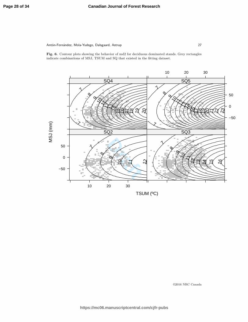
Fig. 6. Contour plots showing the behavior of md2 for deciduous dominated stands. Grey rectanglesindicate combinations of MSJ, TSUM and SQ that existed in the fitting dataset.

TSUM (ºC)

MS

J (m

m)

−50

0

50

10 20 30

7

8

9

10 11 12

SQ2

7

89

10 1112 13 14 15 16

SQ3

7

78

910 11 12 13 14 15 16 17 18 19 20

SQ4

10 20 30

−50

0

50

7

7

89

10 111213 14 15 16 17 18 19 20 21 22 23

SQ5

©2016 NRC Canada

of 34



Draft

28 Can. J. For. Res. Vol. 99, 2016

Fig. 7. Residuals of the best model for each species against the predicted SI. A loess smooth functionwith span smoothing parameter = 2/3 and degree of local polynomial = 1 is shown in black.

Predicted SI (m)

Res

idua

ls (

m)

−10

−5

0

5

10

10 15 20

spruce−10

−5

0

5

10

pine−10

−5

0

5

10

deciduous

©2016 NRC Canada

of 34



Draft


Fig. 8. Distribution of TSUM and MSJ under current climate (C) and RCPs 4.5 projections (F).

TSUM

MS

J

−100

−50

0

50

100

0 10 20 30 40

FFFFF

F FF

FF FFF

FFFF FFF

FF FFF

FF FFFF

F FFFFFF

F FF FFF FFF

FFF FFFF

FFFF FFFF

FFFF F

FFFFFFF F

F FF FFFF FFF

FFFFFFF

F

F

FF F

F

FF

FF

FFF

FFF

FF

FFF F

F FF FFF

FF

FFF FFF F

FFF

F FFFF

F

FFFFF

F FFFFF FFFFFFFF F

F F FF FFF F

F

F

FF

FFFF

F F

F

FF

FF

F

FF

FF

FFF

FFFFFFF

F

F FF

FF FFF

FFFFFF FFFF

F FFF

F

FFF

F F

FF

FFF

FF FF FF

FFF F F

FFFF

FFF

FFF

FF

F

FF

FFF FF

FF F

F

FF

FF FFF F

FF

FF

FF FFFF

FF

FF

F FFFFF

FFFFFFF F F

F FF

FFFF

F

FF

FF

F

F

FF

F

FF

F F FFF FF

FF

F

F FF

FFF

F

F

F FF

F

FFF

F

FFF

FF

FFF FF FF

FF F

F

FF

FF

F

F

FF

FF

F

F

F

FF F FFF

FFF

FF FFFF

FFFF FFF F F FF

FF

FFFF FF

FF

F

FFF

FF FF F

F

FF FFF

FFF

F

F

FF

F

FF FF F

FF

F

FF

FF

F F

F

F

FFF

F

FF

F

F

FFF

FF FFF F

F

FFF

FF

FFFF

FFFFF

F

F

FFF

FFF

FFF

F

FF

F

FFFF

FF

F F

FF F

FF

F

FF FFF F

FFF

F

FFF

F F

FF FF

FFF

F

FF FFF

F FFFFF F

FF F

FF FF

FFF

F

F

FFF F

F F

F FF

F

FF

F

F

FF

F FFFF

FF

F

F

FF FF

FF

FF

FF F

FF

F FFF

F

F

F

FF

FF

F F

F

FF F

F

F

F

F

F

FFF

F

F

FFFF F

FFF

F

F FF

FF

FF

F

FF

FFF

FF

F

F

F

F

F

F

F

F

FF

FF

F F FFF FFFF

F F

FF

F

FFF

FFFF F

FF

FF

FFFF F F

F

FF

FF

F FF F F F FF

FFF

F F

FF

F

F

F

FF

F FF

FF F

FF

FF F

FF F

FFF

FF

FFFFFF

FFFF

F FFF FF F

F

FFFF

FF

FF

F FFF FF FF

FF F

FF

F

F

F

F

FF

FF

FF

FF

FF F

FF

FF

F

FFFF

F FF

F

FF

FF

FF

F

F FF

F FF

FFF

FF F

F FF

FF

FF

FF FFFF

FFFF

FF FFF F

F

FFF F

F F

F

F

FF

FFFF

FF F

F FFFF

FFF

FF

FF

FF

FF

F

F

FF

F

F

F

F

F

FF

F

FF

FF

FF FF F FF

FF

FF

F FFF

F F

F

FF

F

FF

F FF

FF

FFF

FFF

FFFF

FF

FFF

FFFF F

FFF

F

F

FF

FF

F

FFF

FFFF FF

F FF

FFF

FF

FFF

FFF

FFFF

F

F

FF

F

F

F

FF

FF

FFF F

F

F F F

F FFFF

FFFFF

FFFF

FFF

FFFFFFFF

FFFFF

FFFFFFFF FFF

F FFFFFF

FF FFFFFFFFFF FFFF

FF FFF F FFFFF FFF FFF F

FFFFFFF FFF F

FFFF

FFF FF FFFF

FF

FFF

FFFFFFFFFF

F F

F FFFFF FFF FFF FFFFFF FFFFF FF FFF FFFFF

FF FFF FFFFFFFFF FF FFFFF FFF FFF F

FFF FF

FFFF FF FF

F

F FF FF FFF FFFFFF FF F FFFFFFFFF FFFF FFF

FFFF

FFFFF

F

FFFFFFF

FF FFF FFF FFF

F

F

FFF

FFF FF FFFF FFF F FFFFFF FFFF

FF FFF FFF FFF FFFFF F FFFF FFFFFFF

FFFFFF FFFF

FFFFFF F

FFF

FF FFFF

FFFF

FFFFFFF

FFFFFF

F FFF FFFFFF

FFF FFFFF FFFFFF FFFFFF FF

FFF

FF FFFFFF FFFFFFFFFFFFFF

FFFF

FFF

FFFFF FFFFFFFFFFFF FF FFFFFFFFF FF

FFFFFF FFFFFFFFFF FF FF FFFFFFF

FF

FFF

FF

FF

FF

F FFFF

FF

FFF FFFF

F FFFF

FF FFF

FFF FFFF

FF F

FF F FFFFFF

FFFFFF

F FF

FFF

FF FF FFF FFF F

FF FF FFFFFFFFF FF FF FF FFFFFFF FFFFFF FFF FFFFFF FF FFFFFFFFFF FF FFF FF FF FFF FFFF FFFF

FF

F F FFFFF FFF FFF FF FF

F F F FF FF

FFFFF

FFFFFFF FF F FFFFFF

F FFF FFFF FFFF

FF FFFFFFFFFFFFF FFFFFF FFF FFF FFF FFFFFFF

FFFFFFF FFFFF FFF FFFF

FFFF

FFFFFF

FFFF F F

FFFF

FF FF FFFF

FFF FFF

FFFF FF

FF

FF

FFFFFF

FFF

FFF

FF FFF FF F F

FFF

F FFF FFFFFFF

FFFFF F

FFFFFFFF

FF FFF

FF

FF FFF F

FF FFF FFF F F

F FF FFFFFFFF

FFFF

FF FFF

F FFF

FFF

FFFFFF

FF

FF FFFF

FFFFFFFF F FFFF F FFFF

FF FF FF F

FF

FFF

FFFFF

FFFF F

FF FF FFFF

FFF

FF FFF FF

FF F FF

FFF FFF F FF

FFF

FFF FFFFF F FFF FF FFFF FF

FFF FF FFFFF

FF

FF

FF FF F F

FFF

FFFF

F

F FFF F

FF

FFF F

FF FFF

FF FF

FFF

FF FF

FFFFF

FFFFF F FFFFF

F

F

FFF F

FF

FFFF FFFFFFF

F FFFF F

FFF

FFFF F F

FF

FF

F

FFF F FF

FFF

FF F

F

FFFF

FF FF FF

F FFF

FF FFF FFFFF

FFFF F FFF

FFFF

FF FFFF FF

F FFFFFF

FF F F

FFFF FFFFFF FF

FFFFF

F FFFFF FF FF

FFFF

FFF

F FFFFFF F

FF F

F FFF FF

FF

FF

F F FFFFFF FFF F FF

FFF

FF F FFF

F F FF FF

FFFF FF FF FF F

FF FF F FF FFFFFFFF FF FFFFFF FFF FFFFFF F F FFFFF F FF F

FFFFFFF F F FFF F FFFFFF

FF FF

FFFFFF

F F FFF

FF FFFF FF

FFFFFFF FFF FFF

F FFF

FFFF FFFFF F

F

F FF FF

F FFF FFF

FFF

FFFF F FF FFF

FF

FF

FF

F

FF FFFF FFF

FF FFFFFF

FF

FFFFFFFFFFFFF

FFF

FFFF FF

F

F FF F

FFFFF

F F FFFFFFF FFFFF FF FFF F

FF FF

F FF FF F

FF

F

F F FF FFF FF FFFFF FFF FFFFFF F

FFFF

FF FF

FFFFF F F FFFFFF

FFFFF

F

FF

FFFF FF FFFF

FFF FFF FFFFFF

FFF FFFF F FF

FF F

FFFF FF

FF

FFF F FF FFFFFF FFFFFFFFF

FF

F FFFFF F

FFFF F

FFFF

F

F

FF

FFF FFF

FFF

FFFF

FFFF

FFFFFFF

FF FF

FF F F FFF F

FFF

FF

FFF

FFFFF FF F

F

F

F

F

F

F

F

FF F FFF

FF

FFF

FFF

FF

F

F

F F FF FFF FFFF

FFFFF

FFFF

FFF FFFF FF

FFF FFFFF

FFFFFF

FFFF

F FF F

FF F

FF FF F FF FF

FF

FFF F FFFFF

FF

FF FF

FF

FFFF

FF

FF

FF

F

FF

F FFFF

FF FFFF

FFF

F FFF FFFF FFF

F

FFF F

F

FFFFF

F FFF

F FF

FFF

F F

FF

FF F

FFF

FF

FF

FFF

F

F FF

FFF

FF

FFFF

F

FFFF

FFF

FFF F

FFFFFF

F FFF

FF FF

F

FFF

FF F

FF

F FFF FFF

FF

F

F

FFF

FF

FF

FF

FFF

FF

FF

FFFF FF F

FFFFF

FFFFFFF FFF

FFF

FF FF FFF F FF FF

FF

FFFFFFFFFF

F FF

FF

F FF FFF F

F

FF

F

FF

F FF

F F F FFFF FFF

F

FF

FF FF

FFFFFFF

F

FF

F FF FFFFF

FF

FF

F

FFFFFFF

F FFF FF FFFF

F

FF

FF

FFF

F

F

F

FF

FFFF

FF

FFF

FFFFF

FFFFFFFF FFFFFFFFF

F

FFFFF

FFFF FFFFFFFFF FF

F

FFF FFF FFFFFFF FFFFFF FFFFFFF FF

FF

F FFF FFFF FF

FF

FF FF

F FF FFF

FF

FF

FF FFFFFFFFFFFF

FFFFFFFFFFFFFFFF

F

FFFF

FFFFFFF

FFFFFFFFFFF

F FFFFFFFFFFFFFFFF

FFFFFFFFFFFFFFF FFFFFFFFFFFFFFFFFF FFFFFFFFFF FFFF

FFFFFFFFFF

FF F

FFFFF

FFF

FF F

F

F FF F FFFFF

FF

FFFFF FFF F F FFFF

FFF FF

FF

FF F

FFF F FFFF FF

FFFF FFFF

F F FFF F F FF FFFFF

FF

FFF FFF FFF FF FF FFFF

FF FF

FFF

FFFF FF FFF FF FFF

FF

F

FF

F

FFFFFF

FFFFFF FFF FF FFFFF FF

FFFFF FFF F F F

FF FF FF FFFF F FFFFFFFFFF

FFFFFFFFFFFF

FFFFFF

FFFFFFFFF FFFF FFFF FFFFFFFFF

FFFFFFFFFFFFFFFFFFFFF

FFFFFFFFF

FFFFFFFF FFFFFFFFFFFFFFFFFFFFFFF

FFFFFFFFFFF FFFFFFFF

FFFF FFFFFFFFFFFFFFFFFF FFFFF FFFFFFFFFFFFFFFFF FFFF FFFFF FF F F

F F F F FFFFFFFFF

F F FFFFFFF

F FF

F FFFFF FFFF

F

FF FF F

FF

FF FF F

FFF

F FFF FFFFF

FFFFFFF FF FFF F

FFFFF FF FFF

F FF

FFF FFF FFFFFFF

FF F

FFF

FF FF

FF

F

F FF FF FF FF F

FFFF FF

FFFFF

F

FF FF

F FFFFFFF FFF FF

FFF FFFF

FFF

FFF

FFFFFF

FF F

F

F FFF

FF

FF F

FFFFFFFFF

FF FFFFFFFFFFFFFFFFFF

FFFFF

F FFFFFF

FFFFFF FFF FFFFFFFFFFFF FFFFFF FFFFFFF FFFFF FFFFFFF

FFFFF FFF

FFFFFFF

FF

FF

FFF

FFFFFF

FFF

F FFF

FFFF

FFF F

FFFFF FFFF FFF FFF FFFFFFFF FFF FFFFFFFFFFFF F FFFFFFFFFFFFF

FFFFFFF

F FFFFFFF FFFFFFFFF

FF FF FFF FFFFFF FFFFFFFFF

FFF F

FFFF FFF FFF FF FFF FF

FFFFFFF F

FF

F F F FF FF FF FF

FFF FFF FFF F

F FFFFF FFFF

FF

F

FFF

FF FFF

F

F

FFFF

FF

FFFFF

FFFFF FFF

FF FFFFF F FFFF FFFFF

FF

FF FF F

FF FFFFF

F FFFFF

FFFFFFF F

FFF FF

FFFF

FFF FF FF

FF

FFF

FFFFFFFFF FF

FF

F FFF FF

FFFFFFF FFF

F FF FFF FFFFFF FF F FFFF FFFF

FFF

FFFFFFFFFFFF

FFFFFFFF F FF FF

FFFFFFFFF F FFFF FFFFF F

FFFFFFF F

FFF FF FFF FFFF F FFFFFF FFFF F FFF

FFFF

F

FF

FFF FFF

FFFFFFFFF FF F

F F FFFF

FFF F F

F

F FF

FF

FFFFFF

FFF FFF

FF FFFFFFF F FFFFF FFF

FFF FFFFFFFF F

FFFFFF

FF FFFFFFF FF FFFF FFFFF FFF FFF F FFF

FFFF FFF FFFFF FFFFFF FF FFFFFFF

FF FF

FFF FF FFFF FFF

FFF

FF FF FFF F FFF

FFF FF

FF F

FFF

FFFFFF

FF

F FFFFFFFF FFF F

FFF F FF FF

FFFF

FFF

FF FFF FF FFFFFF FFFF FFF FFFFFF FFFFF FF

FFFF F FFFFF FFF FF

FF FF FF FFF FFFFFF

F FFFFFF FFFF

FFFF FFFF F

F FFF FF FFFFFF F

FFFF FFFF FFFF FF FF FF F

F

FF

F FF

FFFFFF FFFFF FFFFFFF F FF FFFF F

FFFFFF F

FF FFFF

FFF

FFFF FF FFFFFF FF

FFFFFF

FF

FFFF FFF

FFFF FF

F FFFFF

FF FFFFFFFFFF FFFFFFFF FFFF FFFFFFFFFFFFF FFF

FFF

FFFFFF

FFFF F

FFFFFFFFF FFFFFFF FFFF FF FF FFF F

FFF FF F FFFFFFFFFFFFFFFFFF FF FFF FFF

FFFFFFF FFFFFFFF FFF FF FFFFF FFFFF

FFF FFF FFF

FFFFF

FFF FFFFFF FFFFFFFF FF FFFF FFFF FFF FFF FF

F FF F

FFF

FF FFFFFFFF FF

FF FF FF

FFF

FF FFF

FFF FFFFF FFFFFF

F FF FFF FFFFFFF FFFF F F

F FF FFFFFF FFF

FFFFFF

FFFFF FF

FFFFFF

FF

FF

FFFF

FFF

FF

FFFF FFFF

FF FF FFFF F

FFF

FF F FF

FFF

FFF FFF FFFFFFFFFF F FFFF F FFFF FFF

FFF

F FF FFFFFF FF

FFFFFFFF FFF

FF FF

FFFFF FFFFF F F

F F FFFFFFF FF

FFF FFFF

FFF FF

FFF FF FF

FFF

FFFFF

FFFF

FFF

FFFFFF FFF F

F FF FFFF FFF FFFFFFFFFFFFFF

FF FF FFFFFF

FFF FFFFF

FFFFFFFFFFFF

FF

FFFFFFF FFF

FFFFFF F FFF FFF FFF F

FFFFFF

FFFFFFFF

FFF

F FFFF F

FF

F FFF

FFF

FF

FFF FFFF

FFF

FFF

F F

F

FFF

F

F

FF

F

FFF

FF

FF

F

FFFFFFFF

FF

FF

FFFFFF FF

FF

FF

FF FF F

FF FFFFFF F

F FF

FFF

F FF

FFFF

FF

FF

FFFF FFFF

FFF F

FF

FFF

FF

FF F FFF FFFFFF F FF

FFFF FF FF

FF

FF

FFFFF

FFF

FFFF FF

FFF FFFFFFFF

FF FF

FFFF FFFF FF

FF FF FF

F FF

F FFFF F FFF FFF FFFF FF

FF

FF

F FFF FFFFF FFFFFFFFFF F F

F FFFF FFF FFFF FFFF FF FF FF FFF FF

FFF

FFF

F

F

FF FFFFF F F FF F

FFFFF

FFFF

FF FF F FFFFFF F

FFFFFFF

FFF FF F FFFF FF F FF FF

FFFFFF F

FFFF FFFF FFFFFFF F FF

FFFFF F FF F FFFFFFF

FFFFFF

FF FF

FFF

FF

FFFFF F

F FFFFF

FFF

F FFF FF FF

FF F FF

FFFFFF FFFF FFFFF F FFF F FFFFF F FFFF FFFFFFFFF FF

FFFFFFFFFF FFFFFF

FFFF

FFFFFF FF FF FFFFF FF FFFFFF F FFF FFF FF FF FFF FFF FFFFFFF FFFF F

F F FFF FF

F FFF

FF FF F FF

FFF

F

FF F FF F

F F FFFFF F F F FFF FFFFFFFF FFF FF FFF F

FF FFFFFF FF FFFFFFFF FFF

F FFF FFFFFFF

FF FFF

FF FFF

FF FF F F F

F FFF

FFF FF F

F FFF FFFFF FF F FFFFFF FFFF FF FFFF

FFFFFF FFFF FFF

FFF FFFFFF F

FFFFFFF

F FFF

FFF

FFFF

F FF FF

FFFFFFFFFFFF

FFFF FFFFF

FF

FFFFFF

FFFFFF FFFF FFFFF

F

F

F

F

F FFFF FFFFFF FFF FFFF

FFFFFFF F FF FF FF FFF

FF

FFFFFFFFFF

FFF FF

FFF

FF F

FF FF FFFFFF FF

FF

FFF

FFFFF

FF FFF F FF F

FFF

F

F FF FF FF FF

FF FF FFFFFF

FFF FFFFF

FF FF FFF F FFF FF FFFFF FFFFFF

F FF FFF F FF FFFF FFF

FFFFF FFF F

FFFF FFFF FFF FF

FFFF

F FF FFF

FF FFFF

FFF FFFFFF

F F FF

FFFFFFF FFFF

FFFF

FF

FF FF F

FF

F

F

FFF

F

FF FF

FFFF FFF

FFFF

FF FF

FF

FFFF

FF

FF

FFFF FFF

FFFFFF

FF

FFFF

FFFFFFFFFFFF FFFF

FFFF FFFFF F

FFF FFFFF

FF

FF

FFF FFFF

FFFF

FF

FFFF FFF

FFFF FF

FF F

F FFF

FFF

FFFFFFF F

F F

FF

FFF

FFFF FFFF

FF

FFFF

F FF

F FFFF

FFFF

F

F

F

FF

FFF

F

FF

FFFF F

FFF FFF

FFF FF FFF

FFFFF

FFF

FFFFFF FF

FFF

F

F

FF

FF

FFF

FF

FFFFFFFFF

F

F

FF

FFFFFFF FF

FFF

FFFF

F FF FFF F

FFF

F FF FFFF

FF

FFF

FFFF

FFF

FF FFF FFF

F

FF

F

FF

FFFF

F

FF

F

FFFFF

FF F

FFFF FF

FF F

FFFF

FF

FF FFF

FF

FFFFFFF

FF FFFF FFFFF FFFFFF FF FFFFFFF

FFFF FFFF FFFFFFFF

FF FFFFF FF FF FFF FFF F FF

FFFFF

FF FFFFFFF FF FFFFFF

FFFFF

FFFFF

F

FFFF FF

FF

FF

F

F

FF

FF

FF

FFF FFFFF

F FF

FFF

F

FFF

FFF

F

FFFFFFFFFFFFFF FF FFFFFFFFF FFFF FFFFFFFF FFFFF FF FFF FFFFFFF FFFFFFF F

FFFFFFF FFFF FFFFFF FF FFFFFFFFFF

FFFFFFF FFFF FF

FFFFFFF

F FFF FFFFFFFFF

FFFFFF FFFF FF FFF

FF FFFFFF F

FF

FFFFFFF FFFF FFF

FFF

FFFFFFFFFFFFFFFF

FFF

FFFFFF

FFFF

F

FFFFF

FFFF FFFF FFF F FFFF FFFFFFF

FFFFFFFFFFFFFFF F FFFFF F

FF FFF FFFF FFFFFFFFFFF

FFF FFFF FFFFFFFF FFF F

FF FF FFF FFFF F FF FF FF FFFF FFFFFF FFFFFF FF FFFFFFFFFF F FF F

FF

FFF

FFF F FF F FF F F

F FFFFFFFF

FFF FF FFF FFFFFFFF FFFFF FFFFFFF FFFF FFFFFFFFFF F FFFFFFFFFFF FFF FF FF FFFFFFFFFF FFFFFF FFFFF F FFF FFFFFF

FFF FFF FFF FFFF F FFFFFFFF FF FFFFFFFFFF FF FFFFF FF FFFFF

FF FF

FF FFF F FFF FFFFF

FF FF

FFFF FF FF

FF F

F

FF

F

FF

FF

FFF FFFFF FFFF

F

FFF FFFF F

FFF

FFFFFFFF

FFF

FF FF FF

FFFF FFF FF

FF

FFFFFFF

F FF FFFF

FF

FF FF FFFFFFF FFFF F

FFFFFFFF

F FFFFFFFF

FFF

F FF FFFFFF FFFFFFF FFF F

FFFFF FF

FFFF F FFF

FFFF

FFF FF FFFFF

FF FFF

FFFF FFFFF FFFFF

FFF FFFF F FFF F FFF FFF

FFFFFFF

F

FF

F

F

F

FFFFF

FFF

F

FFF FF FF FF FFFFF

F

FF

FF

F

FFF

F

FFFF

FF FFF

F

F

F

FFFFF

F

FF

FF

F FF FF

FFFF FF FFFFF FF

FFFF FF

F

FFFFF

FFF

FFFFFFFFF

F FF

FF

F FF

F

FF

FFF

FF

F

FF

FFFF FFF

FFFF FF

F

F

F

FF

FF

FF

F

F

F

F

FFF

FF

FF

F

FF

FF

F

FFFF F

F F FF

FF

FF

FFF FF

F

FF FF F

FF

FF

F

F F

FFF

F

F

FFF

FFF

FFF FFFFF

FFFF FF FFF

F FF FF

FF FF FFF FF

FF

FF

F F FF

FFF

FF F

FFF FF FFFF

FF F FF

FFFF F

F

FF

FFFF

FFF

FFF

F

FF

FFF FFFFF

F

F

FF

FF

F

F

F

FFFF

FFFFF FF

F FFFFFF

F

F

FF

F FFFF

F F

FFF

FF

FF

F

FFF

FF

FFFF

F

F

F FFF

FF

F

FFFFF

F

FF FF

F

FFF

FF F

F

F

FF

F F

F

F

FF

F

F

FFFFFF

FFFFF F FFFF FFFF

FFFFFF FFF FFFF F

FF

F

F

F

F

FF

FF

F FFFFF

FF

FF FFFF

F

F FFF FF

FF

FFFF

F FF

FFFFFF

FF

FFFF F

FFFF F

FFF

F

FF

F

FF F

FF

FFFF

F FF

F FFF FF F F

F

F

F

F

F

F

F

FFFFF

FFFF FFFF FF

FFF

FFFF F F

F F

F

FF

F

F

FF F

F

F

FF FF

FF

F

FF

F FFF F F F

FFFF

F FF FF

F FFF F

F

FFF

F F F

FF

FFF

F

F FFFFF

FF F

FF

FF FFF FF

FFFFF

F FFF

FFFF FFF F

FF

FFF

F

FFF

FFFF FF FF

FFFFF FFF FF

F FF FFF

FFFFFFF

FFFFFFF FFFF

FFF F

FF F

F FFFF

FF

F FFFFFF

F

F

F

FFF

FF

FFFFF

FFF

FF F

F FF FF

FFFF F

F FFF FFF

FF

FF

FF F

F

F

F

FF

FF FFFF F

F FF

FF

F

F FF

F

FF F FFFF

FFF

FF

FF

FF

FFFFF FFFF FF

FF FFF FF

FFF

F FF F F

FFFFFF F

FF

FFF

F FFF FFF F

F

FF

FFF

FFFF

FFFF

FFFF FFFF

FF

F

F FF FF

FF FF FFFFFF

FF

F FFF

F FFFFFF FFF FFF F

FF FF

FF

FF F

F

FFFF FF

F FFF F

FFFFF FF F FF

F FF FFF FFF

FF F FF FFFF FF

FF

FFF

F

FFF

FF F FFFF FFF

FFF

FF

F FF

FFFF F

F F FFF

FF

FFF F

FF

F

FFF

FF

F

FFF

FFFFF

F

FFFFFF

F

FF

FF FFF

FF

FFF

F

F FFFFFFFF

FF

FF

FF FFFF

F F FFF FFFF FF F FF FF FFFFFFFF

FFF FFFFF

F FFF

FF

F

FF

FF

FFF

FF F

FFFFFFF

FFF F

FF

FFF FFFF FFF

F FFFFF

FF

FF FF

FF FF

FF

FFF FFFF FF

F F FFFF FFF F FFFFF FF FFFFFFFF

F FFFFFF FF FFF FFF FFF

F FFFFFF

F F F FF

FF FFFFFF FFF FF

FFFFF

FFF F

F

FFFF

FF

FF

F F

F

F

F

FF FFF

FF

FF

FFF FF

FF

FFF F FFF

FF

FF

FFFF

F

FF

FFF FFF

F

FFFFFF FF

FFFFF FF F

FF

FFFF F

FF

FF FF FFF F F FFFF

F F FFF

FF

FF FFF F

F FFF

F F

FF FFFFF

FFFF FFF F FFFFF

CCCCC

C CC

CC

CC

CCCC

C CCC

CC CCCCC CCCC

C CCCCCC

C CCCCC CCC

CCC CCCCCCCC CCC

CCCCC C

CCCCCCCCC C

CCCCC CCCC

CCCC

CC

C

C

CC C

C

CC

CC

CCC

CCC

CC

CCC C

C CCCC

CCC

CCC C

CC C

CCC

C CCCC

C

CCCCC

C CCCCC CCCCCCCC C

C C CC CCC C

C

C

CC

C CCC

C C

C

CC

CC

C

CC

CC

CCC

CCCCCCC

C

C CC

CC CCCCCCCC

CCCCC

CCC

CC

CC CC C

C

C

CCC

CC CC CC

CCC C C

CCC

C

CCC

CCC

CC

C

CC

CCC C

CC

C C

C

CC

CC CCC C

CC

CC

CC C

CCCC

CC

CC CC

CCC

CCCCC

CC C C

C CC

CCCC

C

CC

CC

C

C

CC

C

C C

C C CCC CC

CC

C

CCC

CC C

C

C

CC

CC

CCC

C

CCC

CC

CCCCC CCCC C

C

CC

CC

C

C

CCC

CC

C

C

CCC CCC

CCC CC CCCC

CCCC CCC C C CC

CC

C CCC CC

CC

C

C CCCC CC C

C

CCCCC

CCC

CC

CC

C

CC CC C

CC

C

CC

CC

C C

C

C

CCCC

CC

CC

CCC

CC CCC C

CCCC

CCCC

CC

CCCCC

C

C

CCC

CC

CCCC

C

CC

C

CCCC

CC

C C

CC C

CC

C

CCCCC C

CCC

C

CCC

CC

CCCCC CC C

CC CCC C CCC

CC C

CC C

CC CC

CCC

C

C

CCC C

C C

CCC

C

CC

C

C

CC

C CCCC

CC

C

C

CC CC

CC

CC

CC C

CC

C CCC

C

C

C

CC

CC

C C

C

CC C

C

C

C

C

C

CCC

C

C

CCCC C

CCC

C

C CC

CC

CC

C

CC

CCC

CC

C

C

C

C

C

C

C

C

CC

CC

C C CCC CCCC

C C

CC

C

CCC

CCC

CC

CCCC

CCCCC C

C

CC

CC

C CC CC CCC

CCC

CC

CC

C

C

C

CC

C CC

CC C

CC C

C CCC C

CCCCC

C

CCCCC

CCCC

C CCC CC C

C

CCCC

CC

CC

C CCC CC C

CC

CC

CC

C

C

C

C

C C

CC

CC

CC

CC C

CC

CC

C

CCC CC CC

C

CC

C

C

CC

C

C CC C CC

CCC

C

C CC C

C

CC

CC

CC C

CCC

CCCC

CCCCC C

C

CCC C

C C

C

C

CC

CCC

CC

C CC CCCC

CCC

CC

CC

CC CC

C

C

CC

C

C

C

C

C

CC

C

CC

CC

CCC

C C CC

CC

CC

C CCC

CCC

CC

C

CC

C CC

CC

C CCCCC

CCCC

CC

CCC

CCC

C C

CCC

C

C

C

CCC

C

CCC

CCCC CCC C

C

CCC

CC

CC CC

CCCCC

CC

C

CC

C

C

C

C

C

C

CCC

C CC

C C C

CC

CCCCCC

CCCCCC

CCCCCCCCCC

CCCCCC

CCCCCCCC C CCCCCCCCC

CC CCCCCCCCCCCCCC

CC CCC C CCCCC CCCCCCC

CCCCCCC CCC C

CCCC

CCC CC CCCCC CC

CC CCCCCCCCCC

C C

C CCCCC CCC CCC CCCCCC CCCCC CC CCCCCCCCCC CCC CCC

CCCCCC CC CCCCCCCC CCC CCC

C CCCC

CC CC CCC

C CC CC CC

C CCCCCC CC C CCCCCC CCC CCCC CC

CCCC CC

CCCCC

CCCCCCC

CC CCC CCC CCC

C

C

CCC CCC

CCCCCC CCC C CCCCCC CCCCCC CCC C

CC CCC CCCCC C CCCC CCCCCCC

CCCCCC CCCC CCCC

CCCC

CCCC CCCC

CCCC

CCCCCC

CCCCCC

CC CCCCCCCC

CC

CC CCCCC CCCCCC CCCCCCCC

CCC

CC CCCCCC CCCCCCCCCCCCCC

CCCC

CCCCCCCC CC

CCCCCCCCCC CC CCCCCCCCC CC

CCCCCC CCCCCCCCCC CC CC CCCCCCCCC

CCCC

C CC

CC C CCCCC

CCCC CCC

C C CC CCCC CCC

CCC CC

CC

CC CCC C CC

CCCCCC

CCCCC CC

CCC

CCCC CCC CCC CCC CC CCCCCCCCC CC CC CC CCCCCCC CCCCCC CCC CCCCCCCC CCCCCCCCCC CC CCC CC CC CCC CCCC C

CCCC

CC C CCCCCCCC CCC CC C

CC C C CC C

CC

CCCCCCCCCCC CC C CCCCCC

CCCC CCCCCCCC

CCCCCCCCCCCCCCC CCCCCC CCC CCCCCCCCCCCCC

CCCCCCC CCCCCCCCCCCC

CCCC

CCCC

CCC

CCC C C CCCC

CC CCCCCC CC

C CCCC

CCC CC

CC

CC CCC CCC

CCC

CCCC

C CCC CC C C

CCC

C C CC CC CCCCCCCCC

C CCC CCCCCCC

C CCCC

CCC CCC C

CC CCC CCC C C

C CCCCC CCC

CC

CCCCCC CC

C

C CCC

CCCC

CCCCCCC CCCCCC

CCCCCCCC C CCCC C CCCCC

C CC CCCC

CC

CCCC

CCCCCCC C

CC CC CCCC C CC CC CCC CC

CC C CC

CCC CCC C CC

CCC

CCC CCCCC C CCCCC CCCCCC

CCC CC CCC

CCC

CCC

CC C

C C CC

CC

CCCC

C

C CCC C

CCCC

C C

CC CCC

CCCC

CCC

CC CC

CCCCCCC

CCC C CCCCCC

CCCC C

C CCCCC CCCC

CCCC CC

CC CC CC

CCCC C C

CC

CC

C

CCC C CC

CCC

CCC

C

CCC

CCC CC CC

C CCC

CC CCC CCCCCCC

CC C CCCCCC

C CC CC CC CCCCCCCCC

CC C CCCCC CCC

CCC CCC

CCCCC C CCCC CC CC

CCCCCCC

C C CCCCC C CC CC CCC CC

CC

CC

C C CCCCCC CC

C C CCCC

C CC C CCC

C C CC CC

CCCC CC CC CCC CCCC CCC CCCCCCCC CC CCCCCC CCC CCCCCC C C CCCCC C CC C

CCCCCCC C C CCC C CCCCCCCC C

CCCCCC

CC C C

CCCC CCCC CC

CCCCCCC CCCCCC

C CCC

CCCC CCCCC C

CC CC C

CC CCC CC

CCCC

CCCC C CCCCC

CC

CC

CC

C

CC CCCC CCC

CC CCCCCC

CC

CCCCCCCCCCCCC

CCC

CCCCCC

CC C

C CCCCC

CC C C

CCCCCC CCCCCCCCCC C

CC CC

C CCCC C

CC

CC C CC CCC CC CCCCC CCC CCCCCCC

CCCC CC CC CCCCC C C CCCCCC

CCCCC

C

CC CCCC CC CCCC

CCC CCC CCCCCC

CCC CCCC C CC C

C CCCCC C

CC

CCCC C CC CCCCC

C CCCCCCCCC

CC

CCC CC C CC CCC C

CCCC

C

C

CC

C CC CCCC

C

C

CCCC

CCCC

CCCCCCC

CC CC

CC C CCCC C

CCC

CC

CCC

CCCCC CC

C

C

CC

C

C

C

C

CC C CCC

CCCCC

CCC

CC

C

C

C C CC CCC CCCCCC

CCCCCCC

CCC CCCC CCCCC CCC

CC CCCCCC

CCCC

C CC C

CC C

CCCC C CC CC C

C CCC C CCCC CC

CC

C CC

CC

CCCC

CC

CC

CC

C

CC

CC

CCC

CC CCCC

CCC

C CCC CCCC C

CCC

C

CC CC

CCC

CC

C CCC

C CC

C

CC

C C

CC

CC C

CCC

C

C

CC

CCC

C

C CC

CCC

CC

CCCC

C

CC

CC

CCC

CCC C

CCCCCC

C CC

CC

C CC

C

CC

C

CC C

CC

C CCC CC C

CC

C

C

CCC

CC

C

CC

C

CCC

C CC

CCCC

C CC C

CCCCC

CCCC CCC CCC

CCC

CC CC CCC C CC

CCC

CC

CCCCCCCCC

C CC

CC

CCC CC

C CC

CC

C

CC

C CCC C C CCCC CC

C

C

CC

CC CC

CCCCCCCC

CC

C CC CCCCC

CC

CC

C

CCCCCCC

C CCC CC

CCCCC

CC

CC

CC

CC

C

C

CC

CC

CCCC

CCC

CCCCCC

CCCCCCC CC

CCCCCCC

C

CCCCC

CCCC CCCCCCCCCCC

C

CCC CCC CCCCCCC CCCCCC CCCCCCC CCCC

C CCC CCCC CCCC

CC CC

C CC CC

CCC

CC

CCCCCCCCCCCCCC

CCCCCCCCCCCCCCCC

CCC

CCCCCCC

CC

CCCCCCCCCCC

C CCCCCCCCCCCCCCC

CCCCCCCCCCCCCCCCCCCCCCCCCCCCCCCCCC CCCCCCCCCC CCCCCCCCCCCC

CCC

C CCCCC

CCC

CC

C CC

C CCCCCCCC

CC

CCCCC CCC C C CCC

CCCCC

C

CC

CC C

CCC CCCCC C

CC

CCC C

CCCCC CCCC C C

C CCCCCCC

CCC CCC CCC CCCC CCCC

CC CC

CCC

CCCC CC CCC CC CCC

CC

CCC

CC

CCCCCC

CCCCC CCC CC CCCCCCC

CCC

CC CCC C C C

CC CC CC CCCC C CCCCCCCCCCCCCCCCCCCCCC

CCCCCCCCCCCCCCC CCCC CCCC CCCCCC

CCC

CCCCCCCCCCCCCCCCCCCCC

CCCCCCCCC

CCCCCCCCCCCCCCCCCCCCCC

CCCCCC

CCCCCCCCCCCCCCCCCCCCCCCCCCCCCCCCCC

CCCCCCCCCC CCCCCCCCCCCCCCCCCCCCCCCCCC CCCCCCC C CC C C CCCCCCCCCC C CCC

CCCC CC C

CC CCC

CC CCCC C

CC CC C

CC

CC CC CCC

CC CCCCCC

CCC

CCCCCC CCCCC C

CCCCC CCCCC

CCC

CCC CCC CCCCCCC

CC C

CCC

CC CC

CC

C

C CC CC CC CC CCCCC C

CCCCCC

C

CC

CC

CCCCC CCC CCCCC CCC CC

CCCC

C

CC

C

CCCCCCCC C

C

C CCCC

CC

C CCCCCC

CCCC

CC CCCCCCCCCCCCCCCCCCC CCCCC C

CCCCCCCCCCC CCC CCCCCCCCCCCC CCCCCC CCCCCCC CCCCC C

CCCCCC

CCCCCC

CCCC

CCCCCC

CCC

CCC

CCCCCC

CCC

CCC C

CCCC

CC

C CCCCCC CCCC CCC CCC CCCCCCCC CCC CCCCCCCCCCCCCCCC

CCCCCCCCCCCCC

CCCCCCCCCCCC CCCCCCCCCCC CC CCCCCCCCC CCCCCCCCCCC CC

CCCC CCC CCC CCCCCCC CCC CCCC CCC

C CC CC CC CC CCCCC C

CC CCC CC CCCCC CCC

CC

C CC

CCCC C

CCC

C

CCCC

CC

CCCCC

CCCCC CC

CCC CCCCC C CCCC CCCCC

CC

CCCC C

CCCCCCCC CCC

CCC CCCCCC CCCC CC

CCCC

CCCCC CC CC CC

CCCCCCCCCCC CCC

C CCCC CC CCCCCC CCC

C CC CCC CCCCCC CC C CCCC CCCC

CCC

CCCCCCCCCCCC

CCCCCCCC C CCC

CCCCCCCCCC CCCCCC

CCCC CCCCCCCC C

CCC CC CCC CCCC CCCCCCCCCCC C CCC

CCCC

C

CC

CCC CC

CCCCCCCCCC CC C

C C CCCC

CCC C C

C

C CC

CC

CCCCCC

CCC CC CCC CCCCCCC C CCCCC CCC

CCCCCCCCCCC C

CCCCCCCC CCCCCCC CC CCCC CCCCC CCCCCC C CCCCCCC CCC CCCCC CCCCCC CC CCCCCCCCC CC

C CC CC CCCC CCCCC

C

CC CC CCC C CCC

CCC CC

CC C

CCC

CCCCCC

CCC CCCCC CCC CCC C

CCC C CC CCCC

CCC

CC

CC CCC CC CCCCCC CCCC CCC CCCCCCCCCCC CC

CCCC C CCC CCCCC CCC

C CC CCCCCCCCCCCCCCCCCC CC

CCCCCC CCCC CCCCCCC CC

CCCC CCCCC CCCC CCCC CC CCCCCC

C CC C C CCCCCC CCCCC CCCCCCC CCC CC

CC CCCCCC

C CCC CCCC

CCC

CCCCCC CCCCCC CC

CCCCCC

CC

CCCC CCCCC

CC CCCCCCC C CC CCCCCCCCCCCCCCCCCC C

CCCCCCCCCCCCCCCC CCC

CCCCCC

CCCCC

CC CCCCCCCC

CCCCCCCCC CCCC CC CC CCC CCCC CCC CCCC

CCCCCCCCCCCCCC CC CCCCCCCCC

CCCCCCCCCCCC CCC CC CCCCC CCCCCC CC CCC CCC

CC CCCCCC CCCCCC CCCCCCCC CC CCCC CCCC CCC CCC C C

C CC CCCC

CC CCCCCCCC CC CC CC C

CCCC

CC CCC CCC CCCCC CCCCCC

C CC CCC CCCCCC

C CCCC C CC CC CCCCC C CCC

CCCCCC

CCCCC CCCCC

CCCC

C CC

CCC CCC

CC

CCC

CC CCCC CCCC CCCC C

CCC CC C C

C

CCC

CCC CCC CCCCCCCCCC C CCCC C CCCC CCCC CC

C CC CCCCCC CC

CCCCCCCC CCC

CC CCCCCCC CCC

CC C CC C CCC

CCCC CC

CCCCCCC

CCC CC

CCC CC CC

CCC

CCCCC

CCCC

CCC

CCCCC

C CCC CC CC CCCCCCCCCCCCCCCCCCCCC CC CC CCCCC

CCCC CCCCC

CCCCCCCCCCCC

CC

CCCCCCC CCC

CCCCCC C CCC CCCCCC C

CCCCCCCCCC

CCCC

CCC

C CCCC CCC

CCCC

CCC

CCCCC CCC

CC

CCC CC

CC

C

C CCC

CC

CC

CCC

CC

CC

C

CCCCCC CC

CCC

C

CCCCCC CC

CC

CC

CC CC CCC CCCCCC C

C CC

CC

CCC

C

CCC CC

C CC

CCCC CCCC

CCC CCC

CCC C

CCC C C

CC CCCCCC C CCCCCC CC CC

CC

CC

CCCCC

CCC

CCCC CC

CCC CCCCCCCCCC CC CC

CC CCCC CCCC C

C CCC C

CC CCCC C C

CC CCC CCCC CCC

CC

CC CCC CCCCC CCCCCCCC

CC C CC CCCC CCC CCCCCCCC CC CC CC CCC CC CCC

CCC

C

C

CC CCCCC C C CCCCC

CCC

CCCC

CCCCC CCCCCC C

CCCCCCCCCC CC CCCCC CCC CC C

CC

CCCCCCC

CCC CCCCCC CCCCC CCC CCCCC C CC C CCC

CCCCC CCCCCC

C CC CCC

CC

CCCCC C C CCCC

CCC

CCCCC CC C

CC

C C CC

CCCCCC CCCC CCCCC C CCC C CCCCC C CCCC CCCCCCCCC CC CCCCCCCCCC CCCCCC

CCCC CCCCCC CC CC CCCCCCC CCCCCC CCCC CCC C

C CCCCC CCCCCCCCCC CCCCCC

C CCC CCC CCC

CC CC C CC

CCC

C

CC C CC CC C CCC

CC C C C CCC CCCCCCCC CCC CC CCC CCC CCCCCC CC CCCCCCCCCCC

C CCC CCCC

CCC

CC CCC

CC CCC

CC CC C C C

C CCC

CCC CC C

CCCC CCCCC CC CCCCCCC C

CCC CC CCCCC CCCCC CCCCCCC

CCC CCCCCC C

CCCCCCC

C CCC

CCC CC

CCC

CC CC

CCCCCCCCCCCC

CCCC CCCCC

CC CC CCCC CCCCCC CCCC CC

CCC

C

C

C

CC CCCC CCCCCC CCC CCCC

CCCCCCCC CC CCCC CCC

CC

CCCCCCCCCC

CCC CC

CC CC

C C

CC CC CCCCCC CC

CC

CCC

CCCCC

CC CCC C CC C

CCC

C

C CC CC CC CC

CC CC CCCCC

CCCC CC

CCCCC CC CCCC CC

C CC CCCCC CCCCCCC CC CC

CC CC CCCC CC

CCCCCC CC

C CC

CCC CCCC CCC CCC

CCC

C CC CCC

CC CCCC

CCC CCCC

CC

CC CC

CCCCC

CC CCCC

CCCC

CC

CC CC C

CC

C

C

CCC

C

CC CC

CCCC CCC

CCC

CCC CC

CCCCC

CC

C

CC

CCCC CCC

CCCCCC

CC

CCCC

CCCCCC

CCCCCC CCCC

CCCC CCCCC C

CCC CCCCC

CC

CC

CCC CCCC

CCCC

CC

CCCC CCC

CCCC CC

CC CC CCC

CCC

CCCCCCCC

C C

CC

CC

C

CCCC CCCC

CC

CC

CCC C

C

C CCCC

CCCC

C

C

C

CC

CCC

C

CC

CCCC C

CCC CCC

CCC C

C CCC

CCCCC

CCC

CCCCCC CC

CCC

C

C

CC

CC

CCC

CC

CCCCCCCCC

C

C

CC

CCCCCCC C

C CCC

CCCC

C CC CCC C

CCC

C CC CCCC

CC

CCC

CCCC

CCC

CC CCC CC

C

C

CC

C

CC

CCCC

C

CC

C

CCCCCC

C CC

CCC CC

CCC

C

CCC

CC

CC CCC

CCCCC

CCCCCC CCCC CCC

CC CCCCCCCC CCCCCCC

CCCCCCCC CCCC

CCCC

CC CC

CCC CC CC CCC CCC C CCCC CCC

CC CCCCCCC

CC CCCCCC

CCCCC

CC

CCC

C

CCCC CC

CC

CC

C

C

CC

CC

CC

CCC CCCCC

C CC

CCC

C

CCC

CCC

C

CCCCCCCCCCCCCC CCCCCCCCCCCCCCCCCCCCCCC CCCCC CCCCC CCCCCCCCCCCCCC C

CCCCCCC CCCC CCCCCC CC CCCCCCCCCCCCCCCCCCCCC CCCCC

CCCCC CCC CCC

CCCCCCCCCCCC CCC

C CC CCCC

CCCCCCC CC CCCC

CCCC CCCC CCCCCC

CCCCCCCC CCCCCCCC

CCC

CCCCCCCC CCC

CC CCC CCCC CCCC CCC C CCCCCCCCCCC

CCCCCCCCCCCCCCC CCCCCC C

CC CCCCCCC CCCCCCCCCCC

CCC CC

CC CCCCCCCC CCC CCC CC CCC CCCC C CC CC CC CCCC CCCCCC CCCCCC CC CCCCCCCCCC CCC C

CC

CCCCCC CCC C C

C C CC CCCC

CCCCCCC CC CCCCCCCCCCC CCCCC CCCCCCC CCCCCCCCCCCCCCC CCCCCCCCCCCCCC CC CC CCCCCCCCCC CCCCCC CCC

CC C CCC CCCCCC

CCC CC

C CCC CCCC C CCCCCCCC CC CCCCCCCCCCCCCCCCC CCCCCCCCC C

CCC

CCC

C CCC CCCCCCC C

CCCCCC

CCCCCC

C

CC

C

CC

CC

CCC CCCCC CCCC

C

CCC CCCC C C

CC CCCCCCCC

CCC

CC CCCC

CCCC CCC CCCC

CCCCCCC

C CC CCCC

CC

CC C

C CCCCCCC CCCC CC

C

CCCCCC

C CCCCCCCCCC CC CC CCCC CC CCCCCCC CCC C

CC CCC CCCCCC C CCC

CCCCCCC CC CCCCC

CCCCC

CCC

CCCCCC CCCCC

CCC CCCC C CCC C CCC CCC

CCCCCCC

C

CC

C

C

C

CCCCC

CCC

C

CCCCC CC CC CCCCC

C

CC

CC

C

CCC

C

CCCC

CC CCC

C

C

C

CCCCC

C

C

C

CC

CC

C CC

CCCC CC CC

CCC CC

CCCC CC

C

CCCCC

CCC

CCCCC

CCC

CC C

C

CC

CC

C

C

CC

CCC

CC

C

CC

CCCC CCC

CCCC CC

C

C

CCC

CC

CC

C

C

C

C

CCC

CC

CC

C

CC

CC

C

CCCC

CCC CC

CC

CC

CCC C

C

C

CC CC C

CC

CC

C

C C

CCCC

C

CCC

CCC

CCCCCCCC CCCC CCCC

CC CC C C

CC CC CCC CCC C C

CC C C

CC

CC CC C

CCC CC CCCCCC C CC

CCCC C

C

CC

CCCC

CCC

CCC

C

CC

CCC CCCCC

C

C

CC

CC

C

CC

CCCC

CCCCC CC

C CCCCCC

C

C

CC

C CCCC

C C

CCC

CC

C

C

C

CCC

C

C

C CCC

C

C

C CCC

CC

C

CCCCC

C

CC C

C

C

CCCCC C

C

CCCC C

C

C

CC

C

C

CCCCCC CCCCC C CCCC CC

CC CCCCCC CCC CCCC C

CC

C

C

C

C

CC

CC

CCC

CCC

CCCC CCCC

C

C CCC CC

CC

CCCC

C CC

CCCCCC

CC

CCCC C

CCCC C

CCC

C

CC

CC

C C

CC

CCCC

CCCCCCC CC C C

C

C

C

C

C

C

C

CCCCC

CCCC CCCC CC

CCC

CCCC

C CC C

C

CC

CC

CC C

C

C

CC CCC

C C

CC

C CCC C C CCC

CC

C CC CC

C CCC C

C

CCC

C C C

CCCCC

C

C CCCCC

CC C

CC

CC CCC CC

CCCCCC C

CCCCCC CCC C

CC

CCC

CCCCCCCC C

C CCCCC

CC CCC CCC C

C CCCCCCCC

CC

CCCCCCC CCC CCC

C CCC CC CCCC

CCC CCC

CCC

C

CC

CCC

CC

CCCC

C CC CCC C

C CC CC

CCCC C

C CCC CCC

CC

CC

CC C

C

C

CC

CCC C

CCC CC C CC

CC

C CC

C

CC C CCC C

CCC

CC

CC

CC

CCCCC CCCCCC CC C

CCCCC

CCC CC C C

CCCCCC C

CC

CCC

C CC

C CCC CC

CC

CCC

CCCC

CCCC

CCC C CCCC CC

C

C CC CCCC CC CCCC

CCCC

C CCC

C CCCCCC CCC CCC C

CC

CC CCC

CCC

CCCC CC

CCCCC

CCCCC CC CCCC CC CCC C

CC

CC C CC CCCCCCC

CCCC

C

CC CCC

CC

CCC CCC

CCCC C

C CC

CCCC CC C CC

CC

C

C CC CC

C

C

CCC

CC

C

CCC

CCCCC

C

CCCCCC

C

CCCCC

CC

CCCC

CC

C CCCCCCCC

CC

CC

CC CCCC

C C CCC CCCC CC C CC CC CCCCCCCC CCC CCCCC

C CCC

CC

C

CC

CCC

CCC

CCC CC CCCC

CCC CCC

CCC CCCCCC

CCCCCC

CC

C

CCC

CCC C

CC

CCCCCCCC C

CC C CCCC CCC C CC

CCC CCCCCCCCCCC CCCCCC CC CCCCCC C

CCC C

CCCCCC C C CC

CC CCCCCCCCC CC

CCCCC

CCC C

CCCCC

C CCCC C

C

C

C

CC CCCC

C CC CCC CCC

CCCC C

CCC

CC

C

C CCCC

CCC

CCCCCCC

CC CCCC CCC

CCCC CC CC

CCC

CC CCCCC CC CCC CC CCCC

C C CCCCC CC CCC C

C C CCC C CC CCC CC

CC CC CCC C CCCCC

©2016 NRC Canada

of 34



Draft

of 34



Draft


Table 1. Number of observations by sitequality and species dominating the stand.The + indicates categories aggregatedwith the next closest category.

Spruce Pine Deciduous

SQ1 + 1183 +SQ2 712 927 433SQ3 1697 540 1061SQ4 915 110 928SQ5 172 + 265Total 3496 2760 2687

©2016 NRC Canada

of 34



Draft

32 Can. J. For. Res. Vol. 99, 2016

Table 2. Definition of the components for each species group. [SQ] indicates when the parametersvary with the site quality parameter.

spruce dominatedP OT π0[SQ]

MODT (1 + exp (−τ1 [SQ] · T SUM + τ0 [SQ]))−1

MODM (1 + exp (−µ1 · MSJ + µ0))−1

pine dominatedP OT π0[SQ]

MODT (1 + exp (−τ1 · T SUM + τ0 [SQ]))−1

MODM ξ−1· µ1/α · ((MSJ − µ0) /α)µ1−1 exp (− ((MSJ − µ0) /α)µ1 )

deciduousP OT π0[SQ]

MODT (1 + exp (−τ1 · T SUM + τ0))−1

MODM ξ−1· µ1/α · ((MSJ − µ0) /α)µ1−1 exp (− ((MSJ − µ0) /α)µ1 )

©2016 NRC Canada

of 34



Draft


Table 3. Parameter estimates and measures of goodness of fit for the twocandidate models for the three species.

spruce pine pine deciduous deciduousParameters md1 md1 md2 md1 md2

π0[SQ1] 9.0797 9.469π0[SQ2] 15.4929 12.7145 13.3917 14.4688 13.041π0[SQ3] 21.7727 13.3343 14.7684 20.1651 18.0119π0[SQ4] 22.9493 16.7999 17.8809 25.3659 22.5634π0[SQ5] 26.1775 29.5949 25.9418τ1 0.1576 0.2068 0.1126 0.1125τ0 3.1924 2.7009τ0[SQ1] 1.8948 2.4028τ0[SQ2] 2.3125 2.9211τ0[SQ3] 1.7933 2.4689τ0[SQ4] 2.5339 3.0053ξ 0.0076 0.0060µ1 1.5042 1.8939µ0 -103.5199 -115.2986α 98.0557 137.4867AIC 17427 13121 12844 12742 12539BIC 17508 13180 12921 12784 12598R2

adj 0.56 0.33 0.40 0.50 0.54RMSE 2.91 2.60 2.47 2.58 2.49

©2016 NRC Canada

of 34



climate sensitive site index models for norway

Documents