1

Climate Risk Management: the Case of Tropical Cyclones

Carolyn W. Changa, Jack S.K. Changb, Kian Guan Limc

JEL classification: G13 Keywords: Tropical cyclones, Catastrophe risk management, Doubly-binomial Tree with stochastic intensity arrival and random time steps; Option Pricing a Department of Finance, California State University, Fullerton b Department of Finance & Law, California State University, Los Angeles c Singapore Management University, Singapore Please forward correspondence to:

Professor Jack S.K. Chang 2858 Bentley Way

Diamond Bar, CA 91765 jskchang@roadrunner.com

2

Climate Risk Management: the Case of Tropical Cyclones

ABSTRACT

Global warming has induced an increasing number of deadly tropical cyclones with a continuing trend.

Developing high-functional climate risk management tools in forecasting, catastrophe modeling, pricing and

hedging is crucial to curtail destruction. We develop a hurricane futures and futures-option pricing model in a

doubly-binomial framework with stochastic news arrival intensity, and a corresponding dynamic market-

consensus forward-looking hurricane forecasting model by using transactional price changes of traded

hurricane derivative contracts as the predictor. Our model can forecast when a hurricane will make landfall,

how destructive it will be, and how this destructive power will evolve from inception to landfall.

3

Introduction

How tropical cyclone activity will respond to human induced global warming is a topic of much popular

interest and scientific debate. This is especially true since Hurricane Katrina, a powerful category 5 storm,

devastated the gulf coast of the United States in 1995 as it passed through. Two frequently asked questions

on global warming and Atlantic hurricanes are i) Have humans already caused a discernible increase in

Atlantic hurricane activity? ii) What changes in Atlantic hurricane activity are expected for the late 21st century,

given the pronounced global warming scenarios from current IPCC (Intergovernmental Panel on Climate

Change) models?

A consensus1 has been developed by the global community of tropical cyclone researchers and

forecasters as represented at the 6th International Workshop on Tropical Cyclones of the WMO (World

Meteorological Organization) in November 2006, indicating that it is likely that greenhouse warming will cause

hurricanes in the coming century to be more destructive by being more intense and having higher rainfall rates

than present-day hurricanes. Among the evidence provided is a comprehensive idealized hurricane intensity

modeling study by Knutson and Tuleya (Journal of Climate, 2004).2 According to this study, an 80 year build-

up of atmospheric CO2 at 1%/yr (compounded) leads to roughly a one-half category increase in potential

hurricane intensity on the Saffir-Simpson scale and an 18% increase in precipitation near the hurricane core. A

1%/yr CO2 increase is an idealized scenario of future climate forcing. An implication is that if the frequency of

tropical cyclones remains the same over the coming century, a greenhouse-gas induced warming may lead to

an increasing risk in the occurrence of highly destructive category-5 storms. This finding has been shared by

many other recent studies, e.g. Emanuel (Nature, 2005). As noted by IPCC, however, there is considerable

uncertainty in projections of future radiative forcing of earth's climate.

In light of the economic impact of global warming and in particular to the insurance industry, the global

investment community has participated in the debate by developing new catastrophe risk management tools.

New 10-day hurricane forecasting tools have been developed by global weather risk specialists like WSI and

Guy Carpenter, and new catastrophe simulation models have been developed by highly skillful, multi-

disciplinary-based specialist vendors like AIR, RMS and EqeCAT. Since Hurricane Katrina, several new

hurricane futures and options contracts have also been developed for trading on exchanges for related parties

to mitigate their extreme weather exposures. In an effort to mitigate the costs of extreme weather events, i.e.

creating building codes, setting insurance premiums and planning for evacuations and relief efforts, federal

agencies have also increased funding to finance weather research programs, aiming at improving the accuracy

of hurricane tracking and intensity forecasts through developing high-resolution dynamic numerical simulation

and prediction, statistical and hybrid models to enhance risk assessment.

In this research, we develop a new pricing and hedging model of hurricane futures and futures options

and up which develop a novel and alternative idea to forecast hurricane activities. Because hurricanes are

complex dynamical systems whose intensities at any given time are affected by a variety of physical processes,

many of which are poorly understood, prevailing individual meteorological and statistical hurricane forecasting

models have been increasingly skillful in tracking hurricanes but not in forecasting their intensities, often

4

yielding inconsistent forecasting results. Since Hurricane Katrina, several new hurricane futures and options

contracts have been developed for trading on exchanges the hurricane futures and options listed on CME

(Chicago Mercantile Exchange) since 2007, the hurricane futures contracts listed on IEM ( Iowa Electronic

Markets) since 2006, and the newly launched (from June 29, 2009) Eurex hurricane futures contracts. Since

traders of these contracts employ all available forecasting models, public or proprietary, to forecast hurricanes

in order to make their pricing and trading decisions, by using the transactional price levels of these contracts as

the predictor and with calibration through the developments of pricing models, one can gain a market

consensus on future hurricane activities out of all of the individual models employed and thus produce a

consistent forecast.

In the finance literature there has been only one research so far that deals with this topic. Kelly et al.

(2009) use the IEM futures data to predict whether a hurricane will or will not make landfall in a given area.

They find that futures price changes are more accurate than the NHC for storms more than five days from

landfall (69% to 54%), but less accurate for storms two days or less from landfall (90% versus 100%). Our

investigation will be based on the more comprehensive CHI contracts3 to predict 1) by using CHI futures data

how destructive a hurricane will be when it makes landfall in a given area, and 2) by using the CME futures

option data when this landfall will occur and how the predicted destructive power will change over time from

inception to landfall.

The rest of our paper is organized as follows: In Section 2, we briefly introduce current hurricane

forecasting models and the CME CHI futures and options contracts. In Section 3, we analyze current hurricane

futures and futures options pricing methodologies to determine which method is most appropriate to employ for

our purpose and then develop our pricing model. In Section 4, we discuss how to extract out the market

consensus view about hurricane activities from transactional CHI futures and futures options prices by using

calibration, and then illustrate our forecast. In Section 5, we expanded the model to allow a hurricane to make

landfall on a random date. In section 6, we conclude the paper and discuss future research directions.

2. Hurricane Forecasting and the CME CHI Futures and Futures Options Contracts

2.1. Hurricane Forecasting

Prevailing hurricane forecast models vary widely in structure and complexity. They can be simple

enough to run in a few seconds on a PC or complex enough to require several hours on a supercomputer.

Dynamical models, also known as numerical models, using high-speed computers to solve the physical

equations of motion governing the atmosphere, are the most complex. The simpler statistical models, in

contrast, use historical relationships between storm behavior and storm-specific details such as location and

date to forecast. Statistical-dynamical models blend both dynamical and statistical techniques by making a

forecast based on established historical relationships between storm behavior and atmospheric variables

provided by dynamical models. Trajectory models move a tropical cyclone (TC) along based on the prevailing

flow obtained from a separate dynamical model. Finally, ensemble or consensus models are created by

5

combining the forecasts from a collection of other models. Table 1 below list most common track and intensity

models employed by NHC (National Hurricane Center) at the US.

______________________________

Insert Table 1 About Here ________________________________

While prevailing models have been increasingly successful in the forecasts of hurricane tracks,

hurricane intensity forecasts are very difficult tasks. Hurricanes are complex dynamical systems whose

intensities at any given time are affected by a variety of physical processes, some of which are internal and

others of which involve interactions between the storms and their environments. Since many of these

processes are poorly understood, there is presently little skill in forecasts of the intensity change of individual

storms. Available computer powers also have limits on their horizontal resolutions to values eyes and eye-walls

properly. It is generally agreed however that there exist thermodynamic limits to intensity that apply in the

absence of significant interaction between storms and their environment. While there remains some

uncertainty about how to calculate such limits, they do appear to provide reasonable upper bounds on the

intensities of observed storms. One particular advantage of limit calculations is they depend only on sea

surface temperature and the vertical temperature structure of the atmosphere, so they are easily calculable

from standard data sets as shown in Figure 1 below.4

______________________________

Insert Figure 1 About Here ________________________________

2.2. The CME CHI Futures and Futures Options Contracts

Following the devastating 2005 hurricane season, the CME Group developed three types of contracts

for hurricane futures and options. The underlying index for various hurricane futures and options on futures

contracts is called the CME Hurricane Index (CHI). It is maintained and calculated by EqeCAT, a leading

authority on extreme-risk modeling. CHI determines a numerical measure of the potential for damage from a

hurricane, using publicly available data from NHC of the National Weather Service. The CHI incorporates

maximum wind velocity and size (radius) of hurricane force winds as illustrated in Figure 2 below and is a

continuous measurement. The commonly used Saffir-Simpson Hurricane Scale (SSHS) classifies hurricanes in

categories from 1 to 5 by considering the velocity but the radius of a hurricane, and thus can not be used to

measure the actual physical impact, making it less than optimal for use by the insurance community and the

public at large. For example, Hurricane Katrina in 2005 was described as a weak category-4 storm at the time

of its landfall but exerted significantly more physical damage than Hurricane Wilma, at one point in its life the

strongest storm on record.

6

______________________________

Insert Figure 2 About Here ________________________________

There are two types of event-driven CHI futures contracts the Eastern USA contract, and the CHI-

Cat-In-A-Box contract that covers the major oil & gas production in the Gulf of Mexico. They trade as follows:

at the beginning of each season, storm names are used from a list, starting with A and ending with Z,

maintained by the World Meteorological Organization. In the event that more than 21 named events occur in a

season, additional storms will take names from the Greek alphabet: Alpha, Beta, Gamma, Delta, and so on.

Named hurricanes must make landfall in the Eastern U.S. (Brownsville, TX to Eastport, ME) for the Eastern

USA contract and Galveston-Mobile area (

South, and the corresponding segment of the U.S. coastline on the North) for the CHI-Cat-In-A-Box contract,

respectively. Trading shall terminate at 9:00 A.M. on the first Exchange business day that is at least two

calendar days following the dissipation or exit from the designated area of a named storm.

All futures contracts remaining open at the termination of trading shall be settled using the reported

respective CHI final value and CHI-Cat-In-A-Box final value (for the latter the maximum calculated CHI value

while the hurricane is within the Box) by EqeCAT. As an initial attempt and to focus on the fundamental issues,

in this research we concentrate on the Eastern USA contract. CME has also offered seasonal, seasonal

maximum and second event seasonal types of contracts. Since these contracts are not straight event-driven

but based on the total, maximum or second event in an entire season, they are irrelevant to our study. Two

types of American-style call options are traded on these futures contracts plain vanilla and binary. Payoff for

the former is the in-the-money amount but $10,000 for the latter.

3. Pricing Hurricane Futures and Futures Options: a Discrete-Time No-Arbitrage martingale Approach

We are interested in using the CHI futures data to predict the expected destructive power of a hurricane

on the expiration date, i.e. when it makes landfall, and using hurricane futures options data to predict when this

date will be, and how this power will evolve over time in three-fold: how likely

news regarding the velocity, size and location of the hurricane that may affect this prediction will arrive in the

next period, and when news does arrive, will the hurricane accentuate or attenuate and to

what extent? In other words, we would need data on transaction arrival as a proxy to news arrival and data on

price changes per transaction arrival to update the prediction. Existent approaches for pricing catastrophe

(CAT hereafter) derivatives include Aase (2001), Cummins and Geman (1995), and Chang, Chang, and Yu

(1996, and CCY hereafter) for pricing CBOT CAT futures and futures call spreads; Bakshi and Madan (2002),

Aase (1999) and Geman and Yor (1997) for pricing CBOT PCS-type cash options; Lee and Yu (2002) and

Loubergé, Kellezi, and Gilli (1999]) for pricing CAT bonds; and Jaimungal and Wang (2006) for pricing

CatEPut. Among them, only CCY is based on both transaction arrival and price changes as explain below.

7

CCY have proposed a unique "randomized operational time" approach to price CAT futures options.

This "randomized operational time" concept, originated in probability theory (Feller (1971), is widely applied in

systems and engineering fields. It dictates that a simple change of time scale will frequently reduce a general

nonstationary process in the usual calendar-time scale to its stationary operational counterpart in a new time

scale dictated by the nature of things. In the finance literature, Clark (1973) first applies this concept to

subordinate stock returns to news arrivals with transaction arrivals being a market proxy, while in the insurance

literature CCY first apply this concept to subordinate CAT futures return to CAT futures transaction arrivals.

This time- change transforms a calendar-time CAT option with stochastic volatility to an isomorphic

transaction-time CAT option with random maturity (to reflect the randomness of transaction arrivals). CCY then

derive a transaction-time option pricing formula as a risk- s (1976) prices over the

the transaction

arrival intensity and the per-transaction futures volatility. Therefore as Geman and Yor (1997) have suggested,

unlike other pricing models that are developed in calendar time and do not incorporate information conveyed in

transaction arrivals, CCY is unique in having the merit of illuminating the information conveyed by transactions.

The CCY methodology is thus the only one that would be relevant to our purpose of calibrating hurricane

activities.

To apply the CCY setup however we encounter four problems: 1) unlike usual transaction arrivals in

financial markets that can be approximately continuous, hurricane news arrivals are sporadic, discrete and

random, 2) CCY only price European-type of options but the CHI futures options are of the American-type with

the early exercise feature, 3) the intensity of catastrophe arrival in CCY is assumed to be constant, however

hurricane arrivals is event-specific and often exhibits time-varying arrival intensity with mean-reversion (see

Levi and Partrat (1991) for a discussion on arrival processes of different types of natural disasters in the

U.S.A.), and 4)

hurricane will make landfall is uncertain. Chang, Chang and Lu (2008) have discretized CCY by employing a

doubly-binomial framework consistent with the compound binomial models of Gerber (1984, 1988) and others

severity (or intensity in the

hurricane forecasting literature) uncertainties in discrete time to circumvent the first two problems. In this

paper, we would develop a generalization of CCL incorporating a discretized mean-reverting stochastic arrival

intensity process to further circumvent the last two problems.

3.1. The Hurricane Futures Process

CME contracts are settled based on the CME Hurricane Index (CHI) values, which measures the

destructive potential of a hurricane. Since this index is physical in nature, its arrival uncertainty should exhibit

no correlation with changes in financial prices, and thus the risks as to when a hurricane will make landfall and

how destructive it will be should be non-systematic (see Hoyt and McCullough, 1999, for empirical evidence

and why this benefit of diversification is one major motivation for portfolio managers to invest in catastrophe

products). This implies price embeds no risk premiums and thus should be a forwarding-looking

8

market prediction of the expected CHI value on the landfall date. Coupled with the increasingly successful

tracking forecast, this also implies when pricing futures options one can circumvent the problem about random

maturity by using the expected maturity (the expected landfall date) without the need to factor the maturity risk

premium into the option price.

To model how the futures price , next we set up a

doubly-binomial model as in Gerber (1984, 1988) and others in the actuarial risk theory to model futures price

changes. The first binomial is to determine if a transaction will arrive and the second to determine if the

corresponding futures price jumps up or down. Thus constructed, the total price change over n time steps is a

random sum of k price changes, where k !"# is the number of transaction arrivals. Transaction arrival is

defined as any news that will impact on the stochastic change of the CHI index value. This construction

essentially defines a subordinated binomial process2; where the sequence of transaction arrivals serves as the

directing process and the subsequent futures price changes from transaction to transaction form the parent

process. In other words, we subordinate binomial futures price changes to random transaction arrivals such

that the futures price will only change when a transaction arrives, irrespective of the passage of calendar time.

The parent process, or the price change from transaction to transaction, is a stationary recombining binomial

tree that will be used later to develop the transaction-time option pricing model.

Subordination collapses the two binomial processes onto to the following trinomial futures price

changes:

uF with probability gh one transaction arrives and the futures price / jumps up at a gross rate u, F F with probability 1-g no transaction arrives and the futures price stays the same, \ dF with probability g(1-h) one transaction arrives and the futures price jumps down at a gross rate d, where F denotes the futures price at the beginning of the period, u and d denote the respective constant up

and down gross jump sizes, g and 1-g denote the respective transaction arrival and no arrival probabilities, and

g and 1-g denote the respective jump up and down probabilities upon an arrival. We let R denote one plus the

riskless rate over one period with the usual regularity condition that u>R>d to prevent riskless arbitrage.

Next we model the changes of hurricane arrival intensity as a mean-reverting Ornstein-Uhlenbeck

process:

(1) ,dZj)dt(mdj

jjjj

where j denotes the speed of adjustment, mj the long-run mean rate, j

2 the instantaneous variance, and Z j

the standard Wiener process. This process exhibits mean-reversion and clustering. Surrounding the time of

news about a hurricane arrival, the intensity takes on higher values to reflect the lumpiness of news arrival, but

it reverts back to the long-run mean level mj after the arrival, and vice-versa. While j itself governs the intensity

of arrival, the speed of adjustment parameter j governs the level of persistence of the intensity process.

9

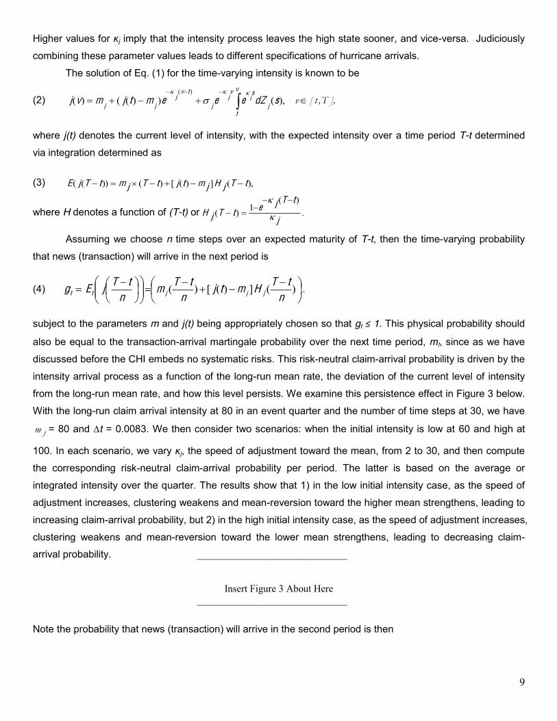
Higher values for j imply that the intensity process leaves the high state sooner, and vice-versa. Judiciously

combining these parameter values leads to different specifications of hurricane arrivals.

The solution of Eq. (1) for the time-varying intensity is known to be

(2) ,)())(()()( v

tj

si

vj

j

tvj

jjsdZeeemtjmvj $"%"&'(

where j(t) denotes the current level of intensity, with the expected intensity over a time period T-t determined

via integration determined as

(3) ),(])([)())(( tTjHjmtjtTjmtTjE

where H denotes a function of (T-t) or .)(

1)(j

tTjetTjH

Assuming we choose n time steps over an expected maturity of T-t, then the time-varying probability

that news (transaction) will arrive in the next period is

(4) )(])([)(n

tTHmtj

n

tTm

n

tTjEg

jjjtt .

subject to the parameters m and j(t) being appropriately chosen so that gt 1. This physical probability should

also be equal to the transaction-arrival martingale probability over the next time period, mt, since as we have

discussed before the CHI embeds no systematic risks. This risk-neutral claim-arrival probability is driven by the

intensity arrival process as a function of the long-run mean rate, the deviation of the current level of intensity

from the long-run mean rate, and how this level persists. We examine this persistence effect in Figure 3 below.

With the long-run claim arrival intensity at 80 in an event quarter and the number of time steps at 30, we have

)* = 80 and t = 0.0083. We then consider two scenarios: when the initial intensity is low at 60 and high at

100. In each scenario, we vary j, the speed of adjustment toward the mean, from 2 to 30, and then compute

the corresponding risk-neutral claim-arrival probability per period. The latter is based on the average or

integrated intensity over the quarter. The results show that 1) in the low initial intensity case, as the speed of

adjustment increases, clustering weakens and mean-reversion toward the higher mean strengthens, leading to

increasing claim-arrival probability, but 2) in the high initial intensity case, as the speed of adjustment increases,

clustering weakens and mean-reversion toward the lower mean strengthens, leading to decreasing claim-

arrival probability. ______________________________

Insert Figure 3 About Here

______________________________

Note the probability that news (transaction) will arrive in the second period is then

10

(5)

.])([)(2])([)(2

21

n

tTHmtj

n

tTm

n

tTHmtj

n

tTm

n

tTjE

n

tTjEm

jjjjjj

ttt

The future forward-looking mt+i and so on, can similarly be calculated as Et{j(i([T-t]/n))}- Et{j([i-1]([T-t]/n))}.

3.2. Risk-Neutralization

Next we apply the discrete-time no-arbitrage martingale pricing methodology to determine the price-

change martingale probability and then develop the risk-neutralized tree. No-arbitrage dictates the following

one-period martingale representations for the futures price:

(6) "+,-./0*,-*/01,*.,

where p and 1-p are the respective equivalent martingale probability measures over one step for the asset

price to move up and down; and m and 1-m are the respective equivalent martingale probability measures over

one step for transaction arrival and non-arrival. As we have shown before m = g.

Solving Eq. (6) and simplifying, we identify the price-change martingale probability:

(7) +1+/. ,

where u (=exp( 1)) and d (= 1/u) are the gross up/down movements of the futures price. This probability

measure resembles closely in format to the standard binomial measure with one difference - u and d here are

determined by the per-transaction volatility 1 only. This is because in our model the futures price will only

jump when a transaction arrives, irrespective of the passage of calendar time.

To summarize, the risk-neutral trinomial tree is obtained by superimposing a jump process on a

standard binomial process such that the movement of the underlying asset at calendar time t over a generic

calendar-time period is modeled by the following trinomial setup:

uFt with probability p1 = mp, / Ft - Ft with probability p2 = 1-m, \ dFt with probability p3 = m(1-p),

where in each period, a transaction arrives with probability m and upon its arrival futures price either jumps up

to uFt with probability p or jumps down to dFt with probability 1-p.

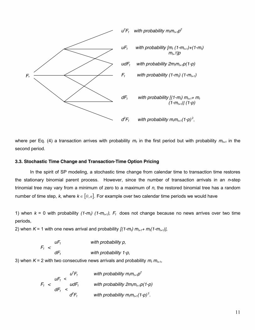
Because the transaction-arrival probability is time-varying however, the futures price evolves over two time

periods as follows:

11

where per Eq. (4) a transaction arrives with probability mt in the first period but with probability mt+1 in the

second period.

3.3. Stochastic Time Change and Transaction-Time Option Pricing

In the spirit of SP modeling, a stochastic time change from calendar time to transaction time restores

the stationary binomial parent process. However, since the number of transaction arrivals in an n-step

trinomial tree may vary from a minimum of zero to a maximum of n, the restored binomial tree has a random

number of time step, k, where k !"# . For example over two calendar time periods we would have

1) when k = 0 with probability (1-mt) (1-mt+1), Ft does not change because no news arrives over two time

periods, 2) when K = 1 with one news arrival and probability [(1-mt) mt+1+ mt(1-mt+1)], uFt with probability p, Ft < dFt with probability 1-p, 3) when K = 2 with two consecutive news arrivals and probability mt mt+1, u2Ft with probability mtmt+1p2 uFt < Ft < udFt with probability 2mtmt+1p(1-p) dFt < d2Ft with probability mtmt+1(1-p) 2.

u2Ft with probability mtmt+1p2 uFt with probability [mt (1-mt+1)+(1-mt) mt+1]p udFt with probability 2mtmt+1p(1-p) Ft with probability (1-mt) (1-mt+1) dFt with probability [(1-mt) mt+1+ mt (1-mt+1)] (1-p) d2Ft with probability mtmt+1(1-p) 2,

Ft F

12

In other words, our task now is to price an isomorphic option with random maturity in transaction time. We

solve this problem by using the Euler equation as a conditional expectation over the transaction arrival

uncertainty. More specifically, the normalized price of an n-period call option can be solved as a random sum

of the arrival-probability-weighted normalized prices of n+1 k-transaction fixed-maturity options (denoted as Ck):

(8) !

#2 %

22

% 345

3-!04 , which simplifies to

(9) !

#22245-!04 ,

where BT is the price of the matching bond, 25 is the transaction-arrival martingale probability measure of k

claim arrivals in n periods, and Ck is the transaction-time American binomial futures call price with k

transactions in maturity. In the case of European options with an N transaction-time-step setup, Ck is

(10) 6

#7

762

722%2 8,+1-70934 ,

where 76-2./072.-:760:7:6-7029 is the N-step martingale probability that the ending futures price level is

,+1 762

72 with ;"

1/+;"<12

26=2

2/ and

22

22 +1

+/. . Since Ck is now priced by the standard binomial model

defined over transaction time but not calendar time, the size of the gross up/down rate now depends on the

transaction-time interval 6=22 .

As in CCY, this pricing model links an option value to the expected intensity of transaction arrival and

the per transaction futures volatility ( 1). As the intensity increases, the tree grows faster, and thus the option

price increases to reflect the larger expected total price volatility, and vice versa. For forecasting we will need

at least three transactional option prices to simultaneously track three parameters: 1) the per transaction

volatility ( 1); 2) the speed of intensity adjustment ( j); and 3) the long-run mean intensity level (mj). By

equation (7), it is seen that 1 also determines u as well as the probability the destructive power will go up, p.

By equation (5), it is seen that, supposing we know current intensity j(t), given j and mj, we can forecast the

probability of news arrival in the future periods, mt+i. Collectively, these values offer a market consensus view

as to how likely a hurricane will change activity level in the next time period, and if it does happen, how likely

the change will be to accentuate and to what new level.

13

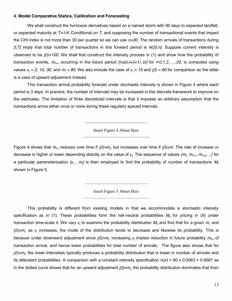
4. Model Comparative Statics, Calibration and Forecasting

We shall construct the hurricane derivatives based on a named storm with 90 days to expected landfall,

or expected maturity at T=1/4. Conditional on T, and supposing the number of transactional events that impact

the CHI index is not more than 30 per quarter so we can use n=30. The random arrivals of transactions during

[t,T] imply that total number of transactions in this forward period is k [0,n]. Suppose current intensity is

observed to be j(t)=100. We shall first construct the intensity process in (1) and show how the probability of

transaction events, mt+i, occurring in the future period [t+i t,t+(i+1)! t] for , is computed using

values j = 2, 15, 30, and mj = 80. We also include the case of j = 15 and j(t) = 60 for comparison as the latter

is a case of upward adjustment instead.

This transaction arrival probability forecast under stochastic intensity is shown in Figure 4 where each

period is 3 days. In practice, the number of intervals may be increased in this discrete framework to improve on

the estimates. The limitation of finite discretized intervals is that it imposes an arbitrary assumption that the

transactions arrive either once or none during these regularly spaced intervals.

______________________________

Insert Figure 4 About Here ________________________________

Figure 4 shows that mt+i reduces over time if j(t)>mj, but increases over time if j(t)<m. The rate of increase or

decrease is higher or lower depending directly on the value of j. The sequence of values {mt, mt+1, mt+2 for

a particular parameterization { j , mj} is then employed to find the probability of number of transactions Mk

shown in Figure 5.

______________________________

Insert Figure 5 About Here

________________________________

This probability is different from existing models in that we accommodate a stochastic intensity

specification as in (1). These probabilities form the risk-neutral probabilities Mk for pricing in (9) under

transaction time-scale k. We vary j to examine the probability distribution Mk and find that for a given mj and

j(t)>mj, as j increases, the mode of the distribution tends to decrease and likewise its probability. This is

because under downward adjustment since j(t)>mj, increasing j implies reduction in future probability mt+i of

transaction arrival, and hence lower probabilities for total number of arrivals. The figure also shows that for

j(t)<mj, the lower intensities typically produces a probability distribution that is lower in number of arrivals and

its attendant probabilities. A comparison with a constant intensity specification mj t = 80 x 0.0083 = 0.6667 as

in the dotted curve shows that for an upward adjustment j(t)>mj, the probability distribution dominates that from

14

using an averaged constant intensity. The situation is converse for the case of downward adjustment where

j(t)<mj.

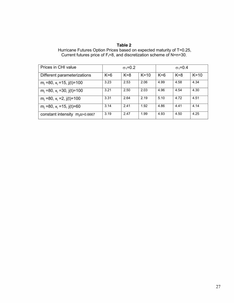
Next, we employ N time-steps to compute the discretized binomial American option prices with random

maturity at transaction times . The transaction-time volatility is fixed at 1=0.2 k/N and separately

1=0.4 k/N in order to evaluate the hurricane futures option no-arbitrage prices. The latter prices are computed

for options with different strike prices at K=6 (in-the-money), K=8 (at-the-money), and K=10 (out-of-the-money)

for a named storm with a traded CHI futures at value Ft=8. For option pricing, an annual riskfree rate of 2% is

assumed. The price results for different sets of parameterizations are shown in Table 2 below. N in principle

should be as large as is computationally feasible, and as N increases, the binomial trees under transaction

maturity should converge to their counterparts under lognormal diffusion. For computational tractability, we

demonstrate the methods here using N=n=30 for all k.

______________________________

Insert Table 2 About Here ________________________________

From Table 2, it is seen that the American-styled hurricane futures option prices increase significantly

with increase in transaction-time volatility 1, with moneyness, and with decrease in j (since j(t)-mj=20 here

indicates an adjustment downward toward the long-run mean). We also compared the American futures option

prices with European ones without early exercise and for cases of low transaction volatilities, the early exercise

premium becomes more significant as American-styled futures options are worth more than European-styled

futures options when the upward price potential becomes less and immediate exercise for positive profit

becomes more valuable. Comparing with the case of long-run constant intensity by setting j(t)=mj=80, it is seen

that whenever j(t)>mj, the American futures option prices will be higher than in the case of constant intensity.

In Figure 6 below, we plot in 3-dimension the hurricane futures option price as a function of j taking the

range 2 to 30, and of 1 under unit transaction time taking the range 0.1 to 0.9. Current futures price is F0=8,

and the strike price is K=8. Maturity is T=1/4. Riskfree interest rate is assumed to be 2% p.a. It is seen that the

price surface increases in 1 and decreases slowly in j (in the case j(t)>mj) for any given option with strike K.

The price surface corresponds to a particular value of mj. Here mj=80 and j(t)=100.

______________________________

Insert Figure 6 About Here ________________________________

15

Any given futures option price level forms a 3-dimensional surface in mj - j " space. Two such surfaces from

two derivatives would form an intersection of a curve at points equivalent to the observed market prices of the

two derivatives. Three derivatives would be able to provide an intersection equivalent to a point in mj - j "

space, and hence providing the implied values of ,,jj

m and j. Once the three parameters are implied at

any trading time t before landfall, they can be used to form a risk-neutral or similarly physical probability

distribution of the CHI values at the expected landfall or maturity time. This is done using the random variable

tiN

ki

kTFduF

~ . We employ all the binomial trees for each k to construct the implied risk-neutral distribution of

TF~

for our forecasting and risk management purposes. For each k, we have n nodal values of FT at T, and thus

N probability values. Conditional on k, these probability values sum to one. Since the probability of observing k

transactions in T is Mk, we have the unconditional probability of nodal value tiN

ki

kTFduF

~ as

.)1()!(!!)()~Pr( iN

kpi

kpiNi

N

kMikPkMT

F

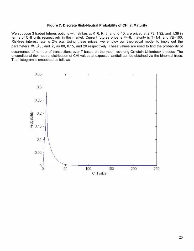
Next Suppose 3 traded futures options with strikes at K=6, K=8, and K=10, are priced at 2.73, 1.92, and

1.38 in terms of CHI units respectively in the market. Using the above theoretical model, we can imply out the

parameters ,,jj

m and j to be 80, 0.15, and 20 respectively, and given j(t)=100 which is assumed to be

observed. Then the risk-neutral distribution of CHI values at expected landfall is shown in Figure 7. This

implied probability distribution provides a forecast of how destructive it will be when it makes landfall with time-

varying arrival probabilities. As the implied probability distribution is tracked over time, it also provides

information on how its expected destructive power will behave over time from inception to landfall. Figure 7

shows that the mean and also mode of the distribution is 8, the current future value, with a probability of about

30%. The distribution is skewed to the right.

______________________________

Insert Figure 7About Here ________________________________

The distribution also provides a way of measuring the risk or probability of hurricane devastation when

the CHI value is expected to exceed certain thresholds. Hurricane Katrina for example made landfall with a

CH

value of 6.9, a mild to medium-sized storm. From the distribution, we can infer that the probability of exceeding

CHI value of 20 is about 4.95% or close to 5%. Hence there is a 5% chance of a serious hurricane hit within 90

days in this example.

In Table 3 below, we also demonstrate a dynamic market-consensus forward-looking forecast as to

how the expected destructive power of a hurricane would evolve from news arrival to news arrival given a

transactional arrival of 30 over 90 days. As shown in the Table, the value in the cell of each node of the

16

binomial tree denotes the expected destructive power in that period. The probability values at the bottom rows

indicate the probability that the news will arrive in the next time period, and p denotes the probability that the

power would increase upon news arrival. By using market-clearing transactional futures and futures options

prices as the predictor, we have developed a transaction-time binomial market-consensus forward-looking

hurricane intensity forecasting model as illustrated.

______________________________

Insert Table 3 About Here ________________________________

5. An Expanded Model with Random Maturity and Forecasting

If we are to model the pricing more completely taking into account the random nature of the landfall or

random optimal stopping of the futures options and futures contract, then we have to introduce an additional

parameter s equivalent to the probability of survival or non-exit of contract each period. This is a minimal model

and can be generalized considering probability of landfall each period or probability of exit of contract to be

dependent over time as the geographical location and direction of the hurricane formation becomes clearer

and closer to the designated areas. With a simplifying assumption of risk-neutral probability s of survival

independent of previous numbers of times of survival, the probability of survival up to and exit at end of

transaction period u is Qu = su (1-s) for -1, and Qn = sn where m is the maximum number of

transaction periods after which survival is zero. We define survival with respect to transaction time. Then using

the framework in (9), the American futures option price can be generalized to

(11) n

kkk

m

n

uCMQC

00

,

where we can define C0 = 0. In principle, n can be a very large number, though in practice, we shall limit n to a

maximum number of plausible transaction periods. A finite n is also necessary for tractable price computation

in this numerical scheme. In this model, there is an additional parameter in s, and so 4 options data must now

be used in order to imply out the various parameters including s. As discussed earlier, the term n

kkk CMnC

0 is a price conditional on maturity T being such that it is the duration of n transaction periods,

and that for the numerical scheme, we can use N=n. Based on the distribution of Qu, the expected maturity

would now be smaller than n.

17

6. Concluding Remarks and Futures Research directions

We develop a hurricane futures and futures-option pricing model in a doubly-binomial framework with

stochastic news arrival intensity, and a corresponding dynamic market-consensus forward-looking hurricane

forecasting model by using transactional price changes of traded hurricane derivative contracts as the predictor.

Our model can forecast when a hurricane will make landfall, how destructive it will be, and how this destructive

power will evolve from inception to landfall. Since from operational forecasting we know that model consensus

is usually superior to any individual model, our market consensus forecast could provide a functional

alternative to prevailing individual models. Since tropical cyclones arrivals are event-specific, one possible

extension is to incorporate additional stylized effects into the futures price process. Empirical verifications to

examine the performance and robustness of the model are also warranted before our predictor is actually

applied.

References

Ané, T. and H. Geman, 2000: Order Flow, Transaction Clock, and Normality of Asset Returns, Journal of Finance, 55, 2259-2284.

Black, F., 1976: The Pricing of Commodity Contracts, Journal of Financial Economics 3, 167-179. Chang, C.W.. J.S.K. Chang, and M.T. Yu, 1996: Pricing catastrophe insurance futures call spreads: a

randomized operational time approach, The Journal of Risk and Insurance, 63, 599-617. Chang, C.W.. J.S.K. Chang, and W. Lu, 2008: Pricing catastrophe options in discrete operational time,

Insurance: Mathematics and Economics, 43, 422-430. Chang, C.W.. J.S.K. Chang, and W. Lu, 2010: Pricing catastrophe options with stochastic claim arrival intensity

in claim time, Journal of Banking & Finance, 34, 24-32. Cox, J.C., S.A. Ross, and M. Rubinstein, 1979: Option Pricing: A Simplified Approach, Journal of Financial

Economics 7, 229-263 Emanuel, K.A., 1987: The dependence of hurricane intensity on climate. Nature, 326, 483-485.

Emanuel, K.A., 1988: The maximum intensity of hurricanes. J. Atmos. Sci., 45, 1143-1155.

Emanuel, K.A., 1995: The behavior of a simple hurricane model using a convective scheme based on subcloud-layer entropy equilibrium. J. Atmos. Sci., 52, 3959-3968.

Emanuel, K., C. DesAutels, C. Holloway, and R. Korty, 2004: Environmental control of tropical cyclone intensity. J. Atmos. Sci., 61, 843-858

Emanuel, K., S. Ravela, E. Vivant, and C. Risi. 2006: A Statistical-Deterministic Approach to Hurricane Risk Assessment. Bull. Amer. Meteor. Soc., 87, 299 314. Online Supplement

18

Emanuel, K. A., 2005: Increasing destructiveness of tropical cyclones over the past 30 years. Nature, 436, 686-688. Online supplement to this paper.

Emanuel, K., 2006: Climate and tropical cyclone activity: A new model downscaling approach. J. Climate, 19, 4797-4802.

Emanuel, K., R. Sundararajan, and J. Williams, 2008: Hurricanes and global warming: Results from downscaling IPCC AR4 simulations. Bull. Amer. Meteor. Soc,, 89, 347-367.

Free, M., M. Bister and K. Emanuel, 2004: Potential intensity of tropical cyclones: Comparison of results from

radiosonde and reanalysis data. J. Climate, 17, 1722-1727 Geman, H., 2005: From Measure Changes to Time Changes in Asset Pricing, Journal of Banking & Finance 29,

2701-2722. Gerber, H.U.,1984: Error Bounds for the Compound Poisson Approximation, Insurance: Mathematics and

Economics 3, 191-194. Gerber, H.U., 1988: Mathematical Fun with the Compound Binomial Process, ASTIN Bulletin 18,161-168. Huang, C.F., and R.H. Litzenberger, 1988, Foundations for Financial Economics, New York: Elsevier Science

Publishing. Kelly D.L., D. Letson, F. Nelson, and D. Nolan, 2009: Evolution of Subjective Hurricane Risk Perception: A

Bayesian Approach, Working Paper, University of Miami Abess Center for Ecosystems Science and Policy.

Jaimungal S., and T. Wang, 2006: Catastrophe Options with Stochastic Interest Rates and Compound Poisson

Losses, Insurance: Mathematics and Economics, 38, 469-483. Knutson T.R., and R.E. Tuleya, 2004: Impact of CO2-Induced Warming on Simulated Hurricane Intensity and

Precipitation: Sensitivity of the Choice of Climate Control and Convective Parameterization, Journal of Climate, 17, 3477-3495.

Lee, J.P., and M.T. Yu, 2002: Pricing Default-Risky CAT Bonds with Moral Hazard and Basis Risk, Journal of

Risk and Insurance 69, 25-44. Levi, C., and C. Partrat, 1991: Statistical Analysis of Natural Events in the United States, ASTIN Bulletin 21,

253-276.

Luo, Z., G. L. Stephens, K. A. Emanuel, D. G. Vane, N. Tourville, and J. M. Haynes, 2008: On the use of CloudSat and MODIS data for estimating hurricane intensity. IEEE Geoscience Remote Sensing Lett., 5, 13-16.

19

End Notes

1 The summary statement is "The surfaces of most tropical oceans have warmed by 0.25-0.5 degree Celsius

during the past several decades. The IPCC considers that the likely primary cause of the rise in global mean

surface temperature in the past 50 years is the increase in greenhouse gas concentrations.......Some recent

scientific articles have reported a large increase in tropical cyclone energy, numbers, and wind-speeds in some

regions during the last few decades in association with warmer sea surface temperatures. Other studies report

that changes in observational techniques and instrumentation are responsible for these increases."

2 Knutson and Tuleya use future climate projections from nine different global climate models and four different

versions of the GFDL (Geophysical Fluid Dynamics Lab) hurricane model. The GFDL hurricane model used is

an enhanced resolution version of the model used to predict hurricanes operationally at NOAA's National

Centers for Environmental Prediction.

3 We focus on the CME contracts since their underlying CME Hurricane Index (CHI) measures the destructive

potential of a hurricane calculated using its intensity and radius, but the Eurex contracts are settled based on

ervices (PCS) unit, while the IEM contracts are based on

tracking - where a given hurricane makes its first landfall.

4 Emanuel et al. (2004) have developed an atmospheric hurricane intensity forecast model that is a simple

axisymmetric-balance model coupled to an equally simple one-dimensional ocean model, phrased in angular

momentum coordinates. Emanuel et al. (2006) graft the above model to a statistical track generation model to

simulate hurricane intensity movement along generated hurricane tracks.

20

Figure 1: A climotological hurricane potential intensity map for monthly mean maximum surface wind speeds (m/s)

Figure 2: The destructive power of a hurricane

21

Figure 3: Risk-Neutral Claim Arrival Probability per period under Constant Averaged Intensity

We assume that the claim arrival intensity follows a mean-reverting Ornstein-Uhlenbeck process and then we examine how the risk-neutral transaction claim-arrival probability, mt, is affected by the deviation of the current level of arrival intensity from the long-run mean rate, j(t)-mj, and the speed of adjustment, j. With the long-run arrival intensity set at 80 and the number of time steps at 30 in an event quarter, we compute mt as a function of j ranging from 2 to 30 in two scenarios: when the initial intensity is low at 60 and high at 100.

22

Figure 4: Transaction Arrival Probability Forecast

We assume that the claim arrival intensity follows a mean-reverting Ornstein-Uhlenbeck process. T=1/4, n=30, mj=80. Different values of k and initial intensity j0 are used to forecast the transaction arrival probability mt+i at future period [t+i t,t+(i+1)! Each period is 3 days in this current setup.

23

Figure 5: Probability of Number of periods of Transaction Arrivals

We assume that the claim arrival intensity follows a mean-reverting Ornstein-Uhlenbeck process. T=1/4, n=30, mj=80. Different values of k and initial intensity j0 are used to forecast the transaction arrival probability mt+i at

The sequence of values {mt, mt+1, mt+2

j , mj} is then employed to find the probability of number of transactions Mk shown below. The case of constant intensity m is derived using mj as per period probability.

24

Figure 6: Weather Futures Call Price Surface

The price surface corresponds to mj=80, j(t)=100, and varying levels of j taking the range 2 to 30, and of 1 under unit transaction time taking the range 0.1 to 0.9. Current futures price is F0=8, and the strike price is K=8. Maturity is T=1/4. Riskfree interest rate is 2% p.a.

25

Figure 7: Discrete Risk-Neutral Probability of CHI at Maturity

We suppose 3 traded futures options with strikes at K=6, K=8, and K=10, are priced at 2.73, 1.92, and 1.38 in terms of CHI units respectively in the market. Current futures price is F0=8, maturity is T=1/4, and j(t)=100. Riskfree interest rate is 2% p.a. Using these prices, we employ our theoretical model to imply out the parameters ,,

jjm and

j as 80, 0.15, and 20 respectively. These values are used to find the probability of

occurrences of number of transactions over T based on the mean-reverting Ornstein-Uhlenbeck process. The unconditional risk-neutral distribution of CHI values at expected landfall can be obtained via the binomial trees. The histogram is smoothed as follows.

26

Table 1

Summary of the mostly commonly used NHC track and intensity models.

intensity the parameters forecast column.

!"#$%&$'()*+,*-./ 0123/4&/ 15+$/ 1*#$6*.$'/78%9:/ ;")"#$,$)'/

<==*(*"6/!>2/=-)$("',/ <329/ / / 1)?@/4.,/!AB%C$-+D5'*("6/36E*F/&5."#*('/9"G-)",-)5/7C3&9:/#-F$6/ C3&9/ HE6,*I6"5$)/)$J*-."6/F5."#*("6/ 9/ 1)?@/4.,/

!AB%>E))*(".$/A$",D$)/K$'$")(D/".F/3-)$("',*.J/H-F$6/7>AK3:! >AK3/ HE,6,*I6"5$)/)$J*-."6/F5."#*("6/ 9/ 1)?@/4.,/!AB%C6-G"6/3-)$("',/B5',$#/7C3B:/ C3B</ HE6,*I6"5$)/J6-G"6/F5."#*("6/ 9/ 1)?@/4.,/

!",*-."6/A$",D$)/B$)L*($/C6-G"6/8.'$#G6$/3-)$("',/B5',$#/7C83B:/ 08H!/ 2-.'$.'E'/ 9/ 1)?@/4.,/M.*,$F/N*.JF-#/H$,/<==*($/#-F$6@/"E,-#",$F/,)"(?$)/7MNH81:/ MNH/ HE6,*I6"5$)/J6-G"6/F5."#*("6/ 9/ 1)?@/4.,/

MNH81/O*,D/'EGP$(,*L$/QE"6*,5/(-.,)-6/"++6*$F/,-/,D$/,)"(?$)/ 8CKK/ HE6,*I6"5$)$F/J6-G"6/F5."#*("6/ 9/ 1)?@/4.,/

!"L5/<+$)",*-."6/C6-G"6/;)$F*(,*-./B5',$#/7!<C0;B:/ !C;B/ HE6,*I6"5$)/J6-G"6/F5."#*("6/ 9/ 1)?@/4.,/!"L5/L$)'*-./-=/C3&9/ C3&!/ HE6,*I6"5$)/)$J*-."6/F5."#*("6/ 9/ 1)?@/4.,/

8.L*)-.#$.,/2"."F"/C6-G"6/8.L*)-.#$.,"6/HE6,*'("6$/H-F$6/ 2H2/ HE6,*I6$L$6/J6-G"6/F5."#*("6/ 9/ 1)?@/4.,/8E)-+$"./2$.,$)/=-)/H$F*E#I)".J$/A$",D$)/3-)$("',*.J/782HA3:/H-F$6/ 8HR/ HE6,*I6"5$)/J6-G"6/F5."#*("6/ 9/ 1)?@/4.,/

S$,"/".F/"FL$(,*-./#-F$6/7'D"66-O/6"5$):/ S0HB/ B*.J6$I6"5$)/,)"P$(,-)5/ 8/ 1)?/S$,"/".F/"FL$(,*-./#-F$6/7#$F*E#/6"5$):/ S0HH/ B*.J6$I6"5$)/,)"P$(,-)5/ 8/ 1)?/

S$,"/".F/"FL$(,*-./#-F$6/7F$$+/6"5$):/ S0H&/ B*.J6$I6"5$)/,)"P$(,-)5/ 8/ 1)?/9*#*,$F/")$"/G")-,)-+*(/#-F$6/ 9S0K/ B*.J6$I6"5$)/)$J*-."6/F5."#*("6/ 8/ 1)?/

!>2TU/70,6".,*(:/ 0TU8/ B,",*',*("6IF5."#*("6/ 8/ 1)?/!>2TV/7;"(*=*(:/ ;TV8/ B,",*',*("6IF5."#*("6/ 8/ 1)?/

294;8KW/726*#",-6-J5/".F/;$)'*',$.($/#-F$6:/ 29;W/ B,",*',*("6/7G"'$6*.$:/ 8/ 1)?/B>43<KW/726*#",-6-J5/".F/;$)'*',$.($/#-F$6:/ B>3W/ B,",*',*("6/7G"'$6*.$:/ 8/ 4.,/

&$("5IB>43<KW/726*#",-6-J5/".F/;$)'*',$.($/#-F$6:/ &B3W/ B,",*',*("6/7G"'$6*.$:/ 8/ 4.,/B,",*',*("6/>E))*(".$/4.,$.'*,5/;)$F*(,*-./B(D$#$/7B>4;B:/ B>4;/ B,",*',*("6IF5."#*("6/ 8/ 4.,/

B>4;B/O*,D/*.6".F/F$("5/ &B>;/ B,",*',*("6IF5."#*("6/ 8/ 4.,/9-J*',*(/C)-O,D/8QE",*-./H-F$6/ 9C8H/ B,",*',*("6IF5."#*("6/ 8/ 4.,/;)$L*-E'/(5(6$/<329@/"FPE',$F/ <324/ 4.,$)+-6",$F/ 8/ 1)?@/4.,/;)$L*-E'/(5(6$/C3&9@/"FPE',$F/ C3&4/ 4.,$)+-6",$FIF5."#*("6/ 8/ 1)?@/4.,/

;)$L*-E'/(5(6$/C3&9@/"FPE',$F/E'*.J/"/L")*"G6$/*.,$.'*,5/-=='$,/(-))$(,*-./,D",/*'/"/=E.(,*-./-=/=-)$("',/,*#$X/!-,$/,D",/=-)/,)"(?@/C>H4/".F/C3&4/")$/

*F$.,*("6/C>H4/ 4.,$)+-6",$FIF5."#*("6/ 8/ 1)?@/4.,/

;)$L*-E'/(5(6$/>AK3@/"FPE',$F/ >A34/ 4.,$)+-6",$FIF5."#*("6/ 8/ 1)?@/4.,/;)$L*-E'/(5(6$/C3B@/"FPE',$F/ C3B4/ 4.,$)+-6",$FIF5."#*("6/ 8/ 1)?@/4.,/;)$L*-E'/(5(6$/MNH@/"FPE',$F/ MNH4/ 4.,$)+-6",$FIF5."#*("6/ 8/ 1)?@/4.,/

;)$L*-E'/(5(6$/8CKK@/"FPE',$F/ 8CK4/ 4.,$)+-6",$FIF5."#*("6/ 8/ 1)?@/4.,/;)$L*-E'/(5(6$/!C;B@/"FPE',$F/ !C;4/ 4.,$)+-6",$FIF5."#*("6/ 8/ 1)?@/4.,/;)$L*-E'/(5(6$/C3&!@/"FPE',$F/ C3!4/ 4.,$)+-6",$FIF5."#*("6/ 8/ 1)?@/4.,/;)$L*-E'/(5(6$/8HR@/"FPE',$F/ 8HR4/ 4.,$)+-6",$FIF5."#*("6/ 8/ 1)?@/4.,/

0L$)"J$/-=/C>H4@/8CK4@/!C;4@/".F/C3B4/ CM!0/ 2-.'$.'E'/ 8/ 1)?/Y$)'*-./-=/CM!0/(-))$(,$F/=-)/#-F$6/G*"'$'/ 2CM!/ 2-))$(,$F/(-.'$.'E'/ 8/ 1)?/

;)$L*-E'/(5(6$/08H!@/"FPE',$F/ 08H4/ 2-.'$.'E'/ 8/ 1)?@/4.,/0L$)"J$/-=/C>H4@/8CK4@/!C;4@/>A34@/".F/C3B4/ 12<!/ 2-.'$.'E'/ 8/ 1)?/

Y$)'*-./-=/12<!/(-))$(,$F/=-)/#-F$6/G*"'$'/ 122!/ 2-))$(,$F/(-.'$.'E'/ 8/ 1)?/0L$)"J$/-=/",/6$"',/Z/-=/C>H4@/8CK4@/!C;4@/>A34@/C3B4@/C3!4@/8HR4/ 1Y2!/ 2-.'$.'E'/ 8/ 1)?/

Y$)'*-./-=/1Y2!/(-))$(,$F/=-)/#-F$6/G*"'$'/ 1Y22/ 2-))$(,$F/(-.'$.'E'/ 8/ 1)?/0L$)"J$/-=/9C8H@/>A34@/C>H4@/".F/&B>;/ 42<!/ 2-.'$.'E'/ 8/ 4.,/

0L$)"J$/-=/",/6$"',/Z/-=/&B>;@/9C8H@/C>H4@/>A34@/".F/C3!4/ 4Y2!/ 2-.'$.'E'/ 8/ 4.,/3BM/BE+$)I$.'$#G6$/ 3BB8/ 2-))$(,$F/(-.'$.'E'/ 8/ 1)?@/4.,/

27

Table 2 Hurricane Futures Option Prices based on expected maturity of T=0.25,

Current futures price of Ft=8, and discretization scheme of N=n=30.

Prices in CHI value 1=0.2 1=0.4

Different parameterizations K=6 K=8 K=10 K=6 K=8 K=10

mj =80, "!=15, j(t)=100 3.23 2.53 2.06 4.99 4.58 4.34

mj =80, " =30, j(t)=100 3.21 2.50 2.03 4.96 4.54 4.30

mj =80, " =2, j(t)=100 3.31 2.64 2.19 5.10 4.72 4.51

mj =80, " =15, j(t)=60 3.14 2.41 1.92 4.86 4.41 4.14

constant intensity mj t=0.6667 3.19 2.47 1.99 4.93 4.50 4.25

28

Table 3 Market-Consensus Forward-Looking Forecast of Hurricane CHI values

using implied parameters m=80, k=20, =0.15; u=1.1618, d=0.8607, p=0.4625. Parameters are conditioned on 30 transaction arrivals over 90 days. Each

Period in the binomial tree below denotes 3 days. /

/

/ / / / / / / / / / / / / / / /[WXT\/

// / / / / / / / / / / / / / /

]WX^^/ W]XZ^//

/ / / / / / / / / / / / / /W]XZ^/ _UX_\/ _VX]]/

// / / / / / / / / / / / /

_UX_\/ _VX]]/ ^WXUW/ ^\XU]//

/ / / / / / / / / / / /_VX]]/ ^WXUW/ ^\XU]/ Z]XW]/ ZZXU]/

// / / / / / / / / / /

^WXUW/ ^\XU]/ Z]XW]/ ZZXU]/ VTX]U/ V]XT_//

/ / / / / / / / / /^\XU]/ Z]XW]/ ZZXU]/ VTX]U/ V]XT_/ V_XWU/ VZXWW/

// / / / / / / / /

Z]XW]/ ZZXU]/ VTX]U/ V]XT_/ V_XWU/ VZXWW/ V\XU\/ TXZT//

/ / / / / / / /ZZXU]/ VTX]U/ V]XT_/ V_XWU/ VZXWW/ V\XU\/ TXZT/ UX\\/ ]XUT/

// / / / / / /

VTX]U/ V]XT_/ V_XWU/ VZXWW/ V\XU\/ TXZT/ UX\\/ ]XUT/ WXT^/ WXV\//

/ / / / / /V]XT_/ V_XWU/ VZXWW/ V\XU\/ TXZT/ UX\\/ ]XUT/ WXT^/ WXV\/ _X^T/ ^X[U/

// / / / /

V_XWU/ VZXWW/ V\XU\/ TXZT/ UX\\/ ]XUT/ WXT^/ WXV\/ _X^T/ ^X[U/ ^XZW/ ZXU\//

/ / / /VZXWW/ V\XU\/ TXZT/ UX\\/ ]XUT/ WXT^/ WXV\/ _X^T/ ^X[U/ ^XZW/ ZXU\/ ZX_V/ ZX\[/

// / /

V\XU\/ TXZT/ UX\\/ ]XUT/ WXT^/ WXV\/ _X^T/ ^X[U/ ^XZW/ ZXU\/ ZX_V/ ZX\[/ VX[T/ VXW_//

/ /TXZT/ UX\\/ ]XUT/ WXT^/ WXV\/ _X^T/ ^X[U/ ^XZW/ ZXU\/ ZX_V/ ZX\[/ VX[T/ VXW_/ VX^Z/ VXV_/

//

UX\\/ ]XUT/ WXT^/ WXV\/ _X^T/ ^X[U/ ^XZW/ ZXU\/ ZX_V/ ZX\[/ VX[T/ VXW_/ VX^Z/ VXV_/ \XTU/ \XU_// +)-G/ \XUZ/ \XU\/ \X[U/ \X[]/ \X[W/ \X[^/ \X[Z/ \X[V/ \X[V/ \X[\/ \X[\/ \X]T/ \X]T/ \X]U/ \X]U/ \X]U// +$)*-F/ \/ V/ Z/ ^/ _/ W/ ]/ [/ U/ T/ V\/ VV/ VZ/ V^/ V_/ VW//

/ / / / / / / / / / / / / /[Z\XV_/

// / / / / / / / / / / / /

]VTXU^/ W^^X_T//

/ / / / / / / / / / / /W^^X_T/ _WTXVU/ ^TWXZZ/

// / / / / / / / / / /

_WTXVU/ ^TWXZZ/ ^_\XV[/ ZTZX[T//

/ / / / / / / / / /^TWXZZ/ ^_\XV[/ ZTZX[T/ ZWZX\\/ ZV]XT\/

// / / / / / / / /

^_\XV[/ ZTZX[T/ ZWZX\\/ ZV]XT\/ VU]X]T/ V]\X]U//

/ / / / / / / /ZTZX[T/ ZWZX\\/ ZV]XT\/ VU]X]T/ V]\X]U/ V^UX^\/ VVTX\_/

// / / / / / /

ZWZX\\/ ZV]XT\/ VU]X]T/ V]\X]U/ V^UX^\/ VVTX\_/ V\ZX_]/ UUXVT//

/ / / / / /ZV]XT\/ VU]X]T/ V]\X]U/ V^UX^\/ VVTX\_/ V\ZX_]/ UUXVT/ [WXT\/ ]WX^^/

// / / / /

VU]X]T/ V]\X]U/ V^UX^\/ VVTX\_/ V\ZX_]/ UUXVT/ [WXT\/ ]WX^^/ W]XZ^/ _UX_\//

/ / / /V]\X]U/ V^UX^\/ VVTX\_/ V\ZX_]/ UUXVT/ [WXT\/ ]WX^^/ W]XZ^/ _UX_\/ _VX]]/ ^WXUW/

// / /

V^UX^\/ VVTX\_/ V\ZX_]/ UUXVT/ [WXT\/ ]WX^^/ W]XZ^/ _UX_\/ _VX]]/ ^WXUW/ ^\XU]/ Z]XW]//

/ /VVTX\_/ V\ZX_]/ UUXVT/ [WXT\/ ]WX^^/ W]XZ^/ _UX_\/ _VX]]/ ^WXUW/ ^\XU]/ Z]XW]/ ZZXU]/ VTX]U/

//

V\ZX_]/ UUXVT/ [WXT\/ ]WX^^/ W]XZ^/ _UX_\/ _VX]]/ ^WXUW/ ^\XU]/ Z]XW]/ ZZXU]/ VTX]U/ V]XT_/ V_XWU// UUXVT/ [WXT\/ ]WX^^/ W]XZ^/ _UX_\/ _VX]]/ ^WXUW/ ^\XU]/ Z]XW]/ ZZXU]/ VTX]U/ V]XT_/ V_XWU/ VZXWW/ V\XU\// ]WX^^/ W]XZ^/ _UX_\/ _VX]]/ ^WXUW/ ^\XU]/ Z]XW]/ ZZXU]/ VTX]U/ V]XT_/ V_XWU/ VZXWW/ V\XU\/ TXZT/ UX\\// _UX_\/ _VX]]/ ^WXUW/ ^\XU]/ Z]XW]/ ZZXU]/ VTX]U/ V]XT_/ V_XWU/ VZXWW/ V\XU\/ TXZT/ UX\\/ ]XUT/ WXT^// ^WXUW/ ^\XU]/ Z]XW]/ ZZXU]/ VTX]U/ V]XT_/ V_XWU/ VZXWW/ V\XU\/ TXZT/ UX\\/ ]XUT/ WXT^/ WXV\/ _X^T// Z]XW]/ ZZXU]/ VTX]U/ V]XT_/ V_XWU/ VZXWW/ V\XU\/ TXZT/ UX\\/ ]XUT/ WXT^/ WXV\/ _X^T/ ^X[U/ ^XZW// VTX]U/ V]XT_/ V_XWU/ VZXWW/ V\XU\/ TXZT/ UX\\/ ]XUT/ WXT^/ WXV\/ _X^T/ ^X[U/ ^XZW/ ZXU\/ ZX_V// V_XWU/ VZXWW/ V\XU\/ TXZT/ UX\\/ ]XUT/ WXT^/ WXV\/ _X^T/ ^X[U/ ^XZW/ ZXU\/ ZX_V/ ZX\[/ VX[T// V\XU\/ TXZT/ UX\\/ ]XUT/ WXT^/ WXV\/ _X^T/ ^X[U/ ^XZW/ ZXU\/ ZX_V/ ZX\[/ VX[T/ VXW_/ VX^Z// UX\\/ ]XUT/ WXT^/ WXV\/ _X^T/ ^X[U/ ^XZW/ ZXU\/ ZX_V/ ZX\[/ VX[T/ VXW_/ VX^Z/ VXV_/ \XTU// WXT^/ WXV\/ _X^T/ ^X[U/ ^XZW/ ZXU\/ ZX_V/ ZX\[/ VX[T/ VXW_/ VX^Z/ VXV_/ \XTU/ \XU_/ \X[^// _X^T/ ^X[U/ ^XZW/ ZXU\/ ZX_V/ ZX\[/ VX[T/ VXW_/ VX^Z/ VXV_/ \XTU/ \XU_/ \X[^/ \X]Z/ \XW_// ^XZW/ ZXU\/ ZX_V/ ZX\[/ VX[T/ VXW_/ VX^Z/ VXV_/ \XTU/ \XU_/ \X[^/ \X]Z/ \XW_/ \X_]/ \X_\// ZX_V/ ZX\[/ VX[T/ VXW_/ VX^Z/ VXV_/ \XTU/ \XU_/ \X[^/ \X]Z/ \XW_/ \X_]/ \X_\/ \X^_/ \X^\// VX[T/ VXW_/ VX^Z/ VXV_/ \XTU/ \XU_/ \X[^/ \X]Z/ \XW_/ \X_]/ \X_\/ \X^_/ \X^\/ \XZW/ \XZZ// VX^Z/ VXV_/ \XTU/ \XU_/ \X[^/ \X]Z/ \XW_/ \X_]/ \X_\/ \X^_/ \X^\/ \XZW/ \XZZ/ \XVT/ \XV]// \XTU/ \XU_/ \X[^/ \X]Z/ \XW_/ \X_]/ \X_\/ \X^_/ \X^\/ \XZW/ \XZZ/ \XVT/ \XV]/ \XV_/ \XVZ// \X[^/ \X]Z/ \XW_/ \X_]/ \X_\/ \X^_/ \X^\/ \XZW/ \XZZ/ \XVT/ \XV]/ \XV_/ \XVZ/ \XV\/ \X\T/

+)-G/ \X]U/ \X]U/ \X][/ \X][/ \X][/ \X][/ \X][/ \X][/ \X][/ \X][/ \X][/ \X][/ \X][/ \X][//+$)*-F/ V]/ V[/ VU/ VT/ Z\/ ZV/ ZZ/ Z^/ Z_/ ZW/ Z]/ Z[/ ZU/ ZT/ ^\/

/

/