University of Chicago Law SchoolChicago UnboundCoase-Sandor Working Paper Series in Law andEconomics Coase-Sandor Institute for Law and Economics

2013

Climate Impacts on Economic Growth as Driversof Uncertainty in the Social Cost of CarbonElisabeth Moyer

Mark D. Woolley

Michael J. Glotter

David A. Weisbach

Follow this and additional works at: https://chicagounbound.uchicago.edu/law_and_economics

Part of the Law Commons

This Working Paper is brought to you for free and open access by the Coase-Sandor Institute for Law and Economics at Chicago Unbound. It has beenaccepted for inclusion in Coase-Sandor Working Paper Series in Law and Economics by an authorized administrator of Chicago Unbound. For moreinformation, please contact unbound@law.uchicago.edu.

Recommended CitationElisabeth Moyer, Mark D. Woolley, Michael J. Glotter & David A. Weisbach, "Climate Impacts on Economic Growth as Drivers ofUncertainty in the Social Cost of Carbon" (Coase-Sandor Institute for Law & Economics Working Paper No. 652, 2013).

CHICAGO COASE-SANDOR INSTITUTE FOR LAW AND ECONOMICS WORKING PAPER NO. 652

(2D SERIES)

Climate Impacts on Economic Growth as Drivers of

Uncertainty in the Social Cost of Carbon

Elisabeth J. Moyer, Mark D. Woolley, Michael J. Glotter, and David A. Weisbach

THE LAW SCHOOL THE UNIVERSITY OF CHICAGO

August 2013

For final published version, see Journal of Legal Studies, vol. 43(2), pp. 401–425

This paper can be downloaded without charge at: The University of Chicago, Institute for Law and Economics Working Paper Series Index:

http://www.law.uchicago.edu/Lawecon/index.html and at the Social Science Research Network Electronic Paper Collection.

Climate impacts on economic growth as drivers ofuncertainty in the social cost of carbon

E.J. Moyer · M.D. Woolley · M.J. Glotter ·D.A. Weisbach

Jul. 31, 2013Submitted to Climatic Change

Abstract One of the central ways that the costs of global warming are incorporatedinto U.S. law is in cost-benefit analysis of federal regulations. In 2010, to standardizeanalyses, an Interagency Working Group (IAWG) established a central estimate ofthe social cost of carbon (SCC) of $21/tCO2 drawn from three commonly-used mod-els of climate change and the global economy. These models produced a relativelynarrow distribution of SCC values, consistent with previous studies. We use one ofthe IAWG models, DICE, to explore which assumptions produce this apparent ro-bustness. SCC values are constrained by a shared feature of model behavior: thoughclimate damages become large as a fraction of economic output, they do not sig-nificantly alter economic trajectories. This persistent growth is inconsistent with thewidely held belief that climate change may have strongly detrimental effects to hu-man society. The discrepancy suggests that the models may not capture the full rangeof possible consequences of climate change. We examine one possibility untested byany previous study, that climate change may directly affect productivity, and find thateven a modest impact of this type increases SCC estimates by many orders of mag-nitude. Our results imply that the SCC is far more uncertain than shown in previousmodeling exercises and highly sensitive to assumptions. Understanding the societalimpact of climate change requires understanding not only the magnitude of losses atany given time but also how those losses may affect future economic growth.

E.J. MoyerDept. of the Geophysical Sciences, University of ChicagoTel.: +1-773-834-2992, fax: +1-773-702-9505, E-mail: moyer@uchicago.edu

M.D. WoolleyLogistics Management Institute (LMI)

M.J. GlotterDept. of the Geophysical Sciences, University of Chicago

D.A. WeisbachLaw School, University of Chicago

2 E.J. Moyer et al.

1 Introduction

One of the central ways that the costs of global warming are incorporated into U.S. lawis through the use of the social cost of carbon (SCC) – the present-value cost of an ad-ditional ton of CO2 emissions – in cost-benefit analysis. Federal agencies are requiredby executive order to assess the costs and the benefits of each significant regulation.In 2009, in an effort to standardize analyses, the Office of Management and Budget(OMB) convened representatives from 12 agencies to participate in an InteragencyWorking Group on the social cost of carbon (IAWG). The IAWG based their studyon three simple, commonly-used integrated assessment models (IAMs) that repre-sent the effects of climate change on the global economy – DICE (Nordhaus, 2008),FUND (Anthoff et al, 2009), and PAGE (Hope, 2006) – and so provides a usefulframework for examining issues in modeling the cost of climate change. The modelswere tuned to match the same socioeconomic scenarios and climate sensitivities, andwere used to predict economic trajectories in the baseline case and with one additionalton of CO2. The SCC is computed as the present value difference in consumption be-tween the two cases. The IAWG’s central SCC estimate (IAWG, 2010) must be usedin cost-benefit analysis of any regulation that affects carbon dioxide emissions.

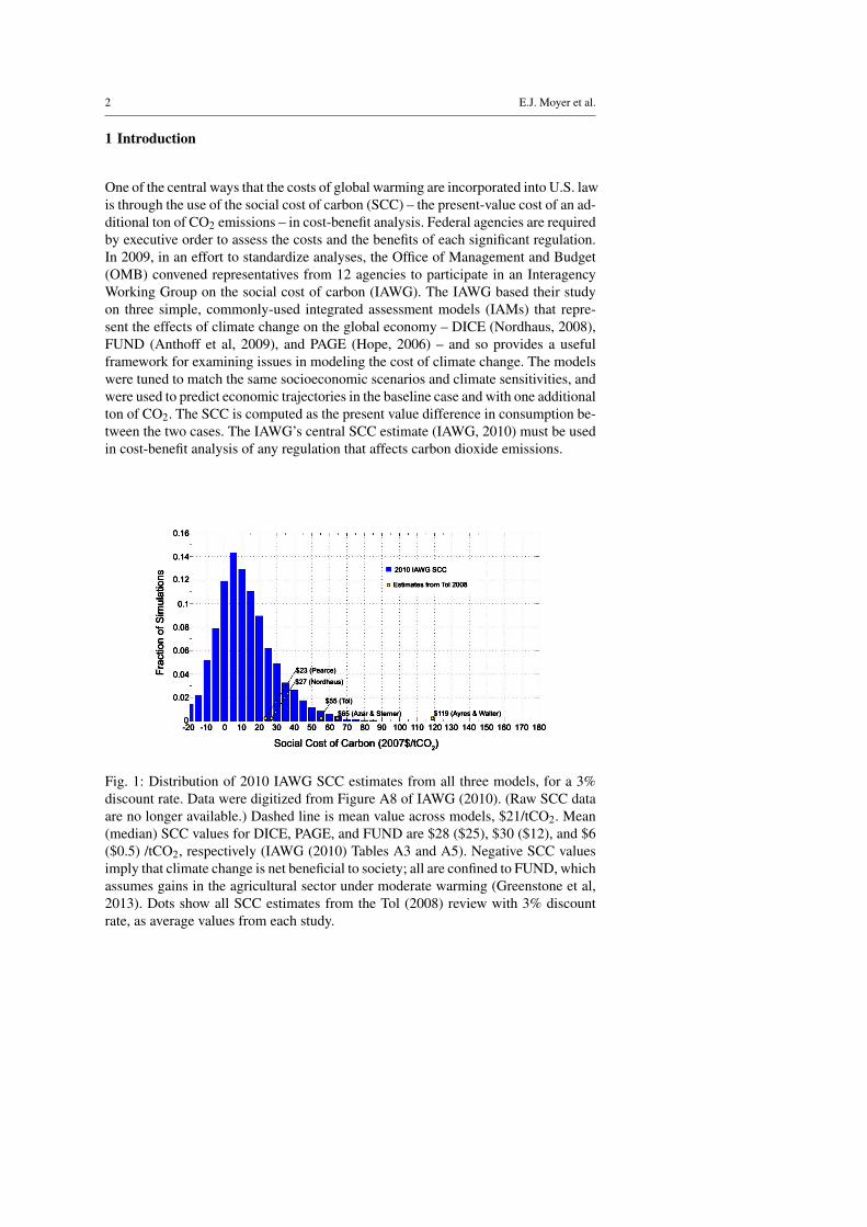
Fig. 1: Distribution of 2010 IAWG SCC estimates from all three models, for a 3%discount rate. Data were digitized from Figure A8 of IAWG (2010). (Raw SCC dataare no longer available.) Dashed line is mean value across models, $21/tCO2. Mean(median) SCC values for DICE, PAGE, and FUND are $28 ($25), $30 ($12), and $6($0.5) /tCO2, respectively (IAWG (2010) Tables A3 and A5). Negative SCC valuesimply that climate change is net beneficial to society; all are confined to FUND, whichassumes gains in the agricultural sector under moderate warming (Greenstone et al,2013). Dots show all SCC estimates from the Tol (2008) review with 3% discountrate, as average values from each study.

Climate effects on growth and the SCC 3

The IAWG’s distribution of SCC values is relatively narrow and consistent withprevious estimates. The distribution with an OMB-required fixed 3% discount rateis right-skewed with a median of ∼ $12/tCO2, a mean of $21/tCO2, and a 95th per-centile value of $68/tCO2 (Fig. 1). A 2008 meta-analysis of SCC estimates showeda similar right-skewed distribution, with values from peer-reviewed studies using a3% discount rate ranging from $23-119/tCO2 (Tol, 2008). Several studies since 2010have revisited the IAWG estimates and generally suggested modest increases (e.g.Johnson and Hope, 2012; Kopp et al, 2012). In 2013, the IAWG used updated modelversions to provide a revised SCC distribution about 50% higher (IAWG (2013), andsee Appendix A for details). Even inclusive of these later studies, the range of SCCvalues is narrow enough to appear inconsistent with the widely held view that thesocietal consequences of climate change over hundreds of years are highly uncertain.

The IAWG models share one notable feature: although climate damages can be-come large as a fraction of output, they do not significantly alter economic trajecto-ries. As an example, we present model output generated with a single IAM, scenario,and climate sensitivity (the DICE model, IMAGE scenario, and 3◦C/CO2 doubling,all discussed further in Section 2). The IMAGE scenario posits that without climatechange, the global economy would grow at an average annual rate of 1.3% (1.2%per capita), yielding per capita income 35 times larger by 2300 (Fig. 2).1 This stronggrowth continues even under basecase CO2 emissions and climate change. Althoughglobal mean temperature rises over 6◦C by 2300, accumulation of wealth is onlyslightly reduced: per capita income rises by a factor of 30 rather than 35. The persis-tence of growth in the face of climate change in DICE and similar models has beennoted by other authors, in particular Weitzman (2011).

0

5

10

15

20

25

30

35

40

Year

GD

P (

rel. to

20

05

)

2000 2100 2200 2300

1

2

3

4

5

6

7

Te

mp

era

ture

ch

an

ge

Before damages After damages Temp. change

2000 2100 2200 23000

5

10

15

Year

%/y

ea

r

Climate damages (% of GDP) GDP/person growth, before damages GDP/person growth, after damages

Fig. 2: Evolution of per capita GDP (left) and per capita annual GDP growth (right)from IAWG DICE-IMAGE, without (black) and with (brown) climate change dam-ages. Left panel includes projected global mean temperature change (red). Rightpanel includes annual GDP losses due to climate damages (red).

Persistent growth leads to SCC values likely too low to justify significant actionto mitigate climate change. Spending to benefit much wealthier future generations

1 In the economic scenarios used by the IAWG, average annual growth rates to 2300 range from 1-1.3%(0.8-1.3% per capita), producing gains in per capita income of 4-6 times by 2100 and 12-40 times by 2300.

4 E.J. Moyer et al.

would need an extraordinary high return to be warranted. In the IMAGE example,with 30x growth by 2300 despite climate change, recommending immediate mitiga-tion spending would be analogous to asking the average current United States house-hold, with an annual family income of $50,000, to transfer wealth to a family with anincome of $1.5 million. Comparison to mitigation costs is also informative. The cen-tral SCC estimate of $21/tCO2 would not likely yield significant transformation ofthe electric sector, even if it were taken as a recommended carbon tax, since the 2010minimum U.S. “price premium” for renewable electricity generation is ∼$22/tCO2(Johnson and Moyer, 2012).2 (See Section 5 for discussion of optimal taxes). TheIAWG process appears to produce a policy recommendation that would not signifi-cantly drive technological evolution for emissions reductions.

Continued economic growth in the face of climate change is inconsistent withmany (admittedly qualitative) statements by experts that climate change may havestrongly detrimental effects to human society. This discrepancy suggests that themodels used in the IAWG process may not capture the full range of possible con-sequences of climate change, i.e. that some aspect of parameter space remains un-sampled. In this study, we explore which aspects of the IAWG process produce theapparent robustness in SCC estimates. In particular, we examine one possibility un-explored by any study, that climate change may directly affect the productivity of theeconomy.3

2 DICE and the Interagency SCC Estimation

We focus on one of the three models used in the IAWG process, DICE (Dynamic In-tegrated Climate-Economy). DICE is an open-source IAM with a long history of usein studies of the costs of global warming (Nordhaus, 1993, 1994, 2007, 2008). Ouranalysis uses the model version modified by the IAWG (“interagency DICE”), whichwas based on the 2007 release (“standard DICE”). We examine only DICE because,of the three IAWG models, it is the only general equilibrium model and thereforethe only one capable of capturing the potential growth impact of climate change thatis the focus of this study. (FUND and PAGE are both partial equilibrium models inwhich economic growth is exogenously specified.) DICE is also open source, widely-known, and based on standard economic theory. For simplicity, we consider only asingle representative socioeconomic trajectory (from IMAGE) and climate sensitivity(3◦C/CO2 doubling, the median value in the distribution used in the IAWG study),but the underlying arguments apply generally.

DICE is based on the Solow-Swan growth model (Solow, 1956; Swan, 1956). Ittreats the entire world as a single region, with output generated by labor and capital

2 $22/tCO2 is the premium commercial windpower in high-wind onshore sites. Commercial dam-basedhydropower is lower-cost.

3 Fankhauser and Tol (2005) consider the possibility that climate change may have an indirect effecton productivity and hence growth. In their model, productivity growth is endogenous and is a function ofthe labor and capital devoted to R&D. Climate change reduces usable output as in DICE, in turn reducingsavings and the capital available to the R&D sector, slowing growth.

Climate effects on growth and the SCC 5

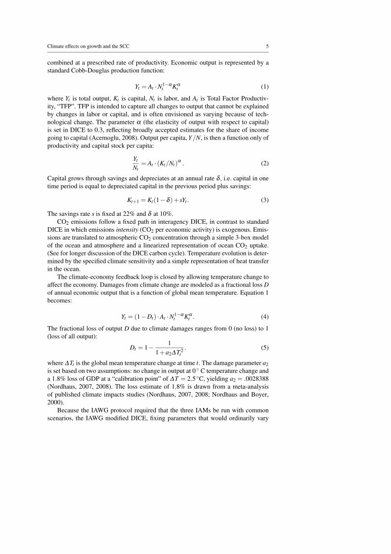
combined at a prescribed rate of productivity. Economic output is represented by astandard Cobb-Douglas production function:

Yt = At ·N1−αt Kα

t (1)

where Yt is total output, Kt is capital, Nt is labor, and At is Total Factor Productiv-ity, “TFP”. TFP is intended to capture all changes to output that cannot be explainedby changes in labor or capital, and is often envisioned as varying because of tech-nological change. The parameter α (the elasticity of output with respect to capital)is set in DICE to 0.3, reflecting broadly accepted estimates for the share of incomegoing to capital (Acemoglu, 2008). Output per capita, Y/N, is then a function only ofproductivity and capital stock per capita:

Yt

Nt= At · (Kt/Nt)

α . (2)

Capital grows through savings and depreciates at an annual rate δ , i.e. capital in onetime period is equal to depreciated capital in the previous period plus savings:

Kt+1 = Kt(1−δ )+ sYt . (3)

The savings rate s is fixed at 22% and δ at 10%.CO2 emissions follow a fixed path in interagency DICE, in contrast to standard

DICE in which emissions intensity (CO2 per economic activity) is exogenous. Emis-sions are translated to atmospheric CO2 concentration through a simple 3-box modelof the ocean and atmosphere and a linearized representation of ocean CO2 uptake.(See for longer discussion of the DICE carbon cycle). Temperature evolution is deter-mined by the specified climate sensitivity and a simple representation of heat transferin the ocean.

The climate-economy feedback loop is closed by allowing temperature change toaffect the economy. Damages from climate change are modeled as a fractional loss Dof annual economic output that is a function of global mean temperature. Equation 1becomes:

Yt = (1−Dt) ·At ·N1−αt Kα

t . (4)

The fractional loss of output D due to climate damages ranges from 0 (no loss) to 1(loss of all output):

Dt = 1− 11+a2∆T 2

t. (5)

where ∆Tt is the global mean temperature change at time t. The damage parameter a2is set based on two assumptions: no change in output at 0 ◦ C temperature change anda 1.8% loss of GDP at a “calibration point” of ∆T = 2.5 ◦C, yielding a2 = .0028388(Nordhaus, 2007, 2008). The loss estimate of 1.8% is drawn from a meta-analysisof published climate impacts studies (Nordhaus, 2007, 2008; Nordhaus and Boyer,2000).

Because the IAWG protocol required that the three IAMs be run with commonscenarios, the IAWG modified DICE, fixing parameters that would ordinarily vary

6 E.J. Moyer et al.

and tuning the model to match specified scenarios of economic output and emissions(2000-2100 forecasts presented at the 2009 Stanford Energy Modeling Forum Ex-ercise 22; see Clarke and Weyant (2009)). Tuning involved constructing exogenousproductivity (TFP) curves to reproduce the prescribed economic evolution. To extendscenarios an additional two hundred years to 2300, the IAWG assumed that popula-tion and GDP growth rates decline linearly from 2100 forward, reaching zero in 2200and 2300, respectively. The resulting assumptions for the IMAGE scenario are shownin Figure 3.

2000 2100 2200 23006

7

8

9

10Population (billions)

2000 2100 2200 23000

0.1

0.2

0.3

0.4Productivity (TFP)

2000 2100 2200 23005

10

15

20Emissions (GtC/year)

2000 2100 2200 23000

0.05

0.1

0.15

0.2Emission Intensity (GtC/$trillion GDP)

Fig. 3: Three exogenous parameters – population, TFP, and annual CO2 emissions– and implied carbon emission intensity for the IMAGE scenario. Productivity in-creases by a factor of 10 between 2000-2300, and emissions intensity falls by a factorof 44. Cumulative emissions during this timeframe are ∼ 4,600 GtC.

To generate pathways of SCC values over time, each model was run with a base-case emissions scenario and sequentially with an additional ton of CO2 emissions ineach scenario year. The SCC in year τ is the net present value of the difference be-tween consumption (output less savings) Cb in the base case and C1 in the case withadditional emissions in year τ:

SCCτ =T

∑t=τ

(Cb−C1)t

(1+ r)t (6)

where r is the discount rate. Because climate damages are assumed nonlinear withglobal mean temperature, the SCC rises over time, approximately doubling between2000 and 2050: damages from an additional ton of CO2 are larger when previouswarming is larger. The IAWG used a fixed discount rate of 3%, required by OMBguidelines, but also reported results for discount rates of 2.5% and 5%. The 2010 SCC

Climate effects on growth and the SCC 7

value derived in our single-scenario, single-climate-sensitivity analysis is similar tothe value obtained by the IAWG with DICE using a distribution over scenarios andparameters: $34/tCO2 vs. $28/tCO2 in IAWG (2010).4

3 Robustness of growth in DICE and alternative specifications of climatedamages

In interagency DICE, economic growth continues despite substantial climate dam-ages because past damages minimally affect economic trajectories. As shown in Fig-ure 2, economic growth remains positive in the year 2300 even when global meantemperature rise exceeds 6 ◦C and the annual loss of output is over 10% of GDP. So-cietal income at this point would have been 35x present without climate change and is30x present with it, but the bulk of that difference is the 10% annual climate-relatedloss of output, which alone would lower income to 31.5x present. The cumulativeeffects of two previous centuries of changed climate make a negligible contribution.

Annual climate losses in DICE are comparable to historical major economicshocks, but the lack of cumulative effects may not be realistic. The Tohoku earth-quake in March 2011 is estimated to have cost Japan 3.3%-5.2% of GDP in recon-struction costs (OECD, 2011), and economic contraction in the U.S. during the GreatDepression was 8.6%, 6.5% and 13.1% in the years 1929-30, 1930-31 and 1931-32,respectively (BEA, 2011). During the Great Depression, economic contractions wereprogressive, with each year’s loss evaluated against that of the previous year, so thatby 1931-32, output was more than 25% lower than in 1928-29. In DICE, by contrast,climate damages in a given year propagate only weakly into the future.

Weak propagation of climate damages in DICE occurs because damages are ap-plied only to output, and can affect growth only indirectly, through two pathways.First, the growth rate dY/dt includes a small term (dD/(1−D))/dt related to year-over-year fractional changes in the damages themselves, which increase as warmingprogresses. Second, climate damages lower savings, because savings are a fixed per-centage of output. Harm from climate change reduces capital available in future years,lowering output in those years. Neither effect is large, however.

We test the robustness of growth in DICE by increasing the magnitude of climatedamages to highly unlikely values, setting losses at the 2.5 ◦C calibration point to15% and 30% of GDP rather than the default 1.8% (Fig. 4a-b). The most extremevalue used is over six times the maximum of the IPCC’s estimated plausible rangeof damages (Pachauri, 2007) and yields annual climate-related losses of over 70% ofGDP by 2300. Even these catastrophic losses do not cause economic contraction. Theassumed exogenous factors driving growth in DICE outweigh any plausible effectsof climate change.

The robustness of growth in DICE suggests that the specification of climate dam-ages may not reflect the full range of possible harms. The model has only four pa-rameters that can be affected by climate change: output Y , capital K, labor N, andproductivity A. In DICE, damages affect only output. Several previous authors have

4 Interagency DICE uses 10-year timesteps beginning with 2005, so our stated 2010 SCC value is theaverage of 2005 and 2015. The IAWG “central” value of $21/tCO2 averages estimates from all models.

8 E.J. Moyer et al.

tested alternative representations of climate damages, including applying them to cap-ital (e.g. Ackerman et al, 2010; Kopp et al, 2012), but all yield economies that growin the face of large climate damages. We consider the possibility that climate changemay reduce productivity growth. While the literature on climate change and technol-ogy includes many studies that consider how endogenously represented technologicalchanges may affect climate (e.g. by promoting the development of low-emission en-ergy sources; for examples see Acemoglu et al, 2012; Gillingham et al, 2008; Popp,2004), no studies have considered the inverse problem, how climate change may di-rectly affect productivity.

Research suggests that TFP levels can be partially explained by human capitalaccumulation, by the quality of government services, and by investment in R&D, allof which may be affected by climate change. (See reviews in Acemoglu, 2008; Barroand Sala-i-Martin, 2003). Some authors have argued that permanent losses of ecosys-tems and the use of capital and labor on adaptation instead of R&D may directlyreduce growth rates (e.g. Pindyck, 2011, 2012). In a world where climate changecauses losses to output, people may also reduce investments in areas that would haveled to greater future output (e.g. education, health care, or public goods), yieldingfuture productivity lower than in a world with no climate change. This indirect effectis analogous to the compounding impact of output losses to the capital stock. (Seealso Fankhauser and Tol, 2005). DICE cannot capture this effect because it does notallow savings to affect TFP, which is entirely exogenous.

The empirical evidence on the impact of climate change on productivity is lim-ited but suggestive. Although temporary weather shocks are not exactly analogousto long-term climate changes, they can inform modeling of climate-related damages.Dell et al (2012) find that temperature shocks lead to several years of lower eco-nomic growth in low-income countries, affecting agricultural yields, industrial out-put, and political institutions, and reducing growth rates temporarily by ∼1.3 per-centage points per ◦C temperature rise. Bansal and Ochoa (2011) find that nationaltemperature shocks reduce growth by 0.9 percentage points per ◦C. Jones and Olken(2010) concur in finding reduced growth in agricultural and light manufacturing ex-ports from poor countries after temperature increases. Of course, for longer-term cli-mate changes, adaptation should result in smaller adverse impacts than those ob-served after short-term weather events. Still, Dell et al (2009) suggest that only halfof the negative short-term impacts of temperature shocks are offset in the long runthrough adaptation.

In this work, we do not try to estimate how damages from climate change willaffect TFP, if at all. Instead, we explore the sensitivity of the SCC estimate to theimplicit assumption in DICE that damages do not affect TFP. To demonstrate thepossible size of the effects, we examine the consequences of two formulations. First,we consider a damage function that imposes a fraction of annual damages on pro-ductivity (and the rest on output) but keeps the year-on-year damages for any givenchange in temperature the same as in the DICE formulation. Climate damages there-fore reduce the level of TFP in any given year. Second, we consider a damage func-tion motivated by a well-known endogenous growth model in which TFP growth isdetermined by the allocation of labor to inventing or manufacturing (Romer, 1990).Climate damages therefore reduce the growth rate of TFP. In both cases, climate ef-

Climate effects on growth and the SCC 9

fects on growth are negative. We do not consider the possibilities suggested by someauthors, that investment in R&D could drive growth that counteract climate damages(Miao and Popp, 2013) or that natural disasters stimulate innovations and actuallyproduce net growth (Skidmore and Toya, 2002). We explore only that part of the un-certainty in SCC values associated with the plausible possibility that climate changemay negatively impact TFP.

3.1 Damages to TFP levels

In our first formulation, we allow a fraction of damages to reduce productivity ratherthan output. We solve for the implicit growth rate of TFP (gAt ) in the exogenouslyspecified path At according to

At+1 = (1+gAt) ·At . (7)

We then allow a fraction f of damages to reduce TFP instead of decreasing output.That is, we specify a new path of TFP, A∗t , that is reduced by climate damages:

A∗t+1 = (1− f ·Dt)(1+gAt) ·A∗t (8)

where A∗0 = A0. The remainder of damages fall on output. Setting DtY = 1− (1−Dt )(1− f ·Dt )

,output equals

Yt = (1−DtY ) ·A∗t ·N1−α

t Kαt .

This modification yields the same single-period fractional loss in consumption (1−Dt ) as in the original specification. The trajectory of economic output is howeverhighly sensitive to assumptions. Applying even a small fraction f of damages to TFPeventually produces negative growth rates, and applying 25% of damages to TFPcauses economic collapse within the analysis timeframe (Fig. 4b-c).

3.2 Damages to TFP growth rates

As a second possibility, we consider a formulation of damages motivated by Romer(1990). That model contains two sectors, an inventing sector and a manufacturingsector; output of the former increases productivity of the latter. We allow damages toapply to both sectors equally. Damages then affect the economy in two ways: theyreduce output of the manufacturing sector the same way they do in DICE – Equation4 still holds – and they reduce output from the inventing sector, which reduces thegrowth rate of TFP according to

A∗t+1 = (1+gAt(1−Dt)) ·A∗t . (9)

This damage function is almost the same as that used by Pindyck (2011, 2012). (SeeAppendix B for derivation.) With this formulation, the DICE climate damages signif-icantly reduce economic growth (Fig. 4b-c, dashed line). During the 300-year timeperiod of our analysis, the effect is roughly similar to applying f = 5% of damages

10 E.J. Moyer et al.

to TFP in Equation 8. Note that with the formulation of Equation 9, as opposed tothat of Equation 8, growth in TFP can vanish but the TFP level cannot shrink, mean-ing climate change cannot produce a severe economic contraction. Equation 9 maytherefore not capture all potential behavior of the climate and economic system. Nev-ertheless, it is informative that climate impacts on TFP can be a natural consequenceof standard economic models.

2000 2100 2200 23000

10

20

30

40GDP per−capita level

GD

P (

rel. to

20

05

)

Before damages 1.8% Damages at 2.5 C (DICE) 15% 30%

a)

2000 2100 2200 2300

−4

−2

0

2

GDP per−capita growth rate

%/year

b)

2000 2100 2200 23000

10

20

30

40

GD

P (

rel. to

20

05

)

Before damages Exogenous TFP (DICE) Damages to TFP growth rate 1% damages to TFP level 5% 10% 25% 50% 100%

c)

2000 2100 2200 2300

−4

−2

0

2

%/year

d)

2000 2100 2200 23000

10

20

30

40

Year

GD

P (

rel. to

20

05

)

Before damages Exogenous TFP (DICE) Damages to TFP growth rate 1% damages to TFP level 5% 10% 25% 50% 100%

e)

2000 2100 2200 2300

−4

−2

0

2

Year

%/year

f )

Fig. 4: Per capita economic output (left) and growth rates (right) in interagency DICE-IMAGE with a variety of climate damages representations. The no-climate-changecase is repeated in black. (a-b): varying damages magnitude at 2.5 ◦C calibrationpoint. Default IAWG value of 1.8% in brown. (c-d): damages applied to the TFP leveland TFP growth rate. (e-f): repeat of c-d with modified model (endogenous emissionsand improved carbon cycle). Model modifications produce slightly lower economicoutput in all but catastrophic cases, where reduced CO2 emissions moderate climatechange and reduce losses instead.

Climate effects on growth and the SCC 11

3.3 Model adjustments required if climate change reduces growth

The assumption that climate change does not reduce growth is so ingrained in intera-gency DICE that the model contains three features that become unrealistic if growthis significantly reduced by climate damages. First, a fixed emissions pathway meansthat if the economy declines, emissions intensity (CO2/GDP) can increase to implau-sible values. Second, a fixed discount rate is inconsistent with theories of the properdiscount rate, which should be sensitive to economic growth. Finally, the DICE car-bon cycle model is valid only on short (decadal) timescales and removes atmosphericCO2 too quickly thereafter. If the discount rate is low because of low growth rates,longer timescales matter. The first of these features would tend to increase SCC val-ues; the second two to decrease them. We therefore adjust the model to correct theseunrealistic assumptions and recalculate economic trajectories (Fig. 4e-f, which repeatthe cases shown in Fig. 4c-d). (For detailed discussion, see Appendices C and D.)Economic evolution remains broadly similar in the modified model, since reducedCO2 emissions under economic decline are offset by slower ocean uptake of CO2.Different damage formulations still produce a wide range of economic outcomes.

4 Comparison of SCC estimates

The varying economic outcomes with different treatments of climate damages pro-duce SCC values that span many orders of magnitude (Table 1 and Fig. 5). Becausethe SCC is also sensitive to the choice of discount rate, a controversial issue, we showSCC calculated with two choices of discount rate parameters: values consistent withthe discussion in IAWG (2010), and values used in Stern report (Stern, 2007) (Param-eters are η = 2, ρ = 1.5%/yr and η = 1, ρ = 0.1%/yr, respectively, in the Ramseyequation rt = η ·gt +ρ , where gt is the growth rate. See Appendix E for discussion.)For either discounting case, the resulting range of SCC values is much larger thanin previous studies (e.g. Johnson and Hope, 2012; Kopp et al, 2012; Tol, 2008). Aswe have retained the same functional form for the magnitude of climate damages,this range reflects only uncertainty about how damages affect growth. Other authorshave discussed alternate functional forms for damages (e.g. Ackerman et al, 2010;Kopp et al, 2012; Weitzman, 2009, 2011). Including those changes would increasethe range of SCC values still further.

The results of this exercise suggest that uncertainty in SCC values due to treat-ment of damages is comparable to that due to treatment of discounting. SCC valuesrise approximately exponentially with fraction of damages to TFP. The rate of risedepends on η , with higher η producing greater sensitivity to damage assumptions:when damages are low and growth rates positive, harms to future generations areweighted less; when the economy contracts, harms to future generations are weightedmore (Fig. 5). In all cases with damages to TFP levels, growth rates become negativeand either produce negative discount rates or would do so if the analysis timeframewere extended. Once the discount rate is negative, the present value of future dam-ages grows exponentially with the time until damages occur. The exact SCC value istherefore an artifact of the time horizon of the analysis and would increase with the

12 E.J. Moyer et al.

Damages treatment 2010 SCC Value ($2007/tCO2)IAWG model Modified model Modified model

fixed discounting η = 2, ρ = 1% η = 1, ρ = 0.1%

DICE damages 34 16 2101% damages to TFP level 51 22 4405% damages to TFP level 110 54 1,300Damages to TFP growth rate 160 72 1,50010% damages to TFP level 160 130 2,20025% damages to TFP level 250 1,600 4,80050% damages to TFP level 320 100,000 8,000

Table 1: Selected 2010 SCC estimates from unmodified and modified interagencyDICE-IMAGE (climate sensitivity 3◦C/CO2 doubling), under different formulationsof climate damages and assumptions about discounting. Discounting with η = 2,ρ = 1%/yr produces greater sensitivity to damage treatment. With DICE damages,SCC is lower than in the fixed-discounting case because the endogenous discount rateis initially larger than 3%. Cases with damages to TFP eventually produce negativediscount rates, so SCC estimates would grow if analysis were extended past 2300.

0 10 20 30 40 50 60 70 80 90 10010

0

101

102

103

104

105

106

107

108

109

20

10

SC

C (

$2

00

7)

Share (%) of Damages to TFP Level

Modified model, η=2, ρ=1%

Modified model, η=1, ρ=0.1%

Fig. 5: The 2010 SCC from modified DICE under varying assumptions regardingdamages to productivity, for two alternate specifications of discount rate: η = 2 andρ = 1% (solid) and η = 1, ρ = 0.1% (dashed). The SCC rises exponentially withgreater climate impacts to the determinants of growth. Higher η produces higherSCC values in simulations dominated by negative growth rates, because future harmsare weighted more.

length of time considered. The SCC values we show are several orders of magnitudehigher than IAWG estimates, but even so are limited by termination of the analysis in

Climate effects on growth and the SCC 13

2300. Very high SCC values indicate large potential harms from climate change, butare difficult to interpret quantitatively.

The extreme cases of climate-related damages that we explore may not be real-istic, as neither standard nor interagency DICE contains the flexibility to representbehavior in circumstances of economic contraction. Adjustments to savings rates donot alter the qualitative results, but our simple damage formulation may not real-istically capture economic consequences given adaptive actions. The work here issimply an exploration of uncertainty across possible parameter values in the simpleIAM frameworks commonly used. The importance of growth effects means that morerealistic representations are needed.

5 Discussion and Conclusions

Our results imply that the SCC is far more uncertain than shown in the IAWG re-port or in previous modeling exercises, and that narrow distributions appear to be anartifact of model assumptions. Prior models do not allow the SCC to affect growth(except indirectly) and the SCC is sensitive to this restriction. While we take no viewon whether climate change will affect growth, it is not likely that these effects can beruled out a priori, and they should not be precluded by choices made in the structureof the model. If climate change reduces TFP levels or growth rate, the direction ofthe changes in the SCC value are uniformly upward. It is therefore possible that theSCC was underestimated by the IAWG and by previous studies.

In the model studied here, even a modest impact of climate damages on produc-tivity can cause the SCC to grow so large as to limit its usefulness as a guide topolicymaking. The SCC is evaluated under business-as-usual assumptions, which as-sume no policy-driven mitigation. Incremental damages will be maximal in this case,because incremental losses grow with the degree of climate change. A large SCCvalue signifies large potential gains from mitigation, but if current mitigation is farfrom optimal, the SCC would exceed the value of a carbon tax in the context of acomprehensive policy. The optimal carbon tax is set instead to that point where themarginal mitigation costs are equal to the marginal benefits of reduced harms fromclimate change.5 In the case of very high SCC values, formulating regulatory pol-icy based on the SCC rather than the optimal tax would impose undue costs. (Nosensible policymaker, for example, would apply an SCC value of $100,000/tCO2 incost-benefit analysis if all emissions could be eliminated for $100/tCO2.)

Understanding how interactions between climate change and economic growthproduce uncertainty in the SCC provides insight into past controversies over the ap-propriate choice of discount rate. Proponents of an “empirical” discount rate arguefor use of values similar to observed market rates while proponents of an “ethical”discount rate argue for lower values to place greater weight on the welfare of fu-ture generations. Our results suggest that the roots of the dispute may lie not in theprinciples of discounting but in differing implicit assumptions about climate dam-ages combined with counterintuitive IAM behavior. A 3% discount rate means that

5 The optimal carbon tax would be estimated by an analysis in which mitigation efforts are incremen-tally increased until the cost of any additional mitigation no longer exceeds the resulting additional benefit.

14 E.J. Moyer et al.

harms after 2100 are essentially disregarded. But it is not unethical to disregard cli-mate harms to future generations if those harms are small. The SCC values from theIAWG process are not unreasonable if the assumptions in the IAWG models are true,and future generations are many times richer despite climate change. If impacts arecatastrophic instead, then standard economic analysis would indicate a low discountrate and would produce a recommendation of significant policy action. (See reviewin Kaplow et al, 2010). In this study, SCC values become very high if climate changereduces future wealth significantly by reducing the growth rate. It is possible that thedebate over discounting results not from a difference in ethics but from an unrecog-nized dispute over the treatment of climate impacts.

Finally, our results suggest that the greatest uncertainty in the cost of climatechange may lie not in the magnitude of losses at any given time but in how thoselosses affect growth. DICE damage magnitudes are broadly consistent with the esti-mate in the IPCC Fourth Assessment Report that a temperature change of 4 ◦C wouldcause global mean losses between 1 and 5% of GDP (Pachauri, 2007). Both the phys-ical and social science communities have shown increasing interest in studying poten-tial climate impacts, and many current studies focus on better quantifying economiclosses. Our exploration of SCC sensitivities suggests that a higher research priorityshould be understanding how those losses relate to growth. The importance of growthis well understood more generally; even small differences in growth rates can producelarge differences in wellbeing over time. As in the rest of economics, growth effectsmay be the predominant factor governing the impacts of climate change.

Acknowledgements The authors thank the many organizers of and participants in the 2010/2011 EPA/DOEWorkshops on the social cost of carbon for discussion that informed this work, and Martin Weitzman,Gilbert Metcalf, Alex Marten, Michael Canes, David Anthoff, and Nicholas Stern for helpful commentson the manuscript. Misung Ahn derived the growth rate representation based on the Romer model, andJoe Zhu digitized the 2010 and 2013 SCC estimates from IAWG reports. This research was performed aspart of the Center for Robust Decision-making on Climate and Energy Policy (RDCEP) at the Universityof Chicago, funded by a grant from the National Science Foundation (NSF) Decision Making Under Un-certainty program (#SES-0951576). M.W. acknowledges support from the Logistics Management Instituteand M.G. from an NSF Graduate Fellowship (#DGE-1144082).

References

Acemoglu D (2008) Introduction to Modern Economic Growth. Princeton UniversityPress

Acemoglu D, Aghion P, Bursztyn L, Hemous D (2012) The environment and directedtechnical change. American Economic Review 102(1):131–166

Ackerman F, Stanton E, Bueno R (2010) Fat tails, exponents, extreme uncertainty:Simulating catastrophe in DICE. Ecological Economics 69(8):1657–1665

Aghion P, Howitt PW (2009) The Economics of Growth. The MIT PressAnthoff D, Tol RS, Yohe GW (2009) Risk aversion, time preference, and the social

cost of carbon. Environmental Research Letters 4Archer D, Eby M, Brovkin V, Ridgwell A, Cao L, Mikolajewicz U, Caldeira K, Mat-

sumoto K, Munhoven G, Montenegro A, et al (2009) Atmospheric lifetime of fossilfuel carbon dioxide. Annual Review of Earth and Planetary Sciences 37:117–134

Climate effects on growth and the SCC 15

Bansal R, Ochoa M (2011) Temperature, aggregate risk, and expected returns. NBERWorking Paper 17575

Barro RJ, Sala-i-Martin X (2003) Economic Growth, 2nd edn. The MIT PressBEA (2011) National Income and Product Analysis Table 1.1.1.

http://www.bea.gov/iTable/index nipa.cfm, accessed 2012-03-19Bolin B, Eriksson E (1959) Distribution of matter in the sea and the atmosphere. The

Atmosphere and the Sea in MotionClarke L, Weyant J (2009) Introduction to the EMF 22 special issue on climate change

control scenarios. Energy Economics 31:S63Dell M, Jones BF, Olken BA (2009) Temperature and income: Reconciling new cross-

sectional and panel estimates. American Economic Review Papers and Proceed-ings 99(2):198–204

Dell M, Jones BF, Olken BA (2012) Temperature shocks and economic growth: Ev-idence from the last half century. American Economic Journal: Macroeconomics4(3):66–95

Fankhauser S, Tol RSJ (2005) On climate change and economic growth. Resourceand Energy Economics 27(1):1–17

Gillingham K, Newell RG, Pizer WA (2008) Modeling endogenous technical changefor climate policy analysis. Energy Economics 30(6):2734–2753

Glotter M, Pierrehumbert R, Elliott J, Moyer E (2013) A simple carbon cycle repre-sentation for economic and policy analyses. In preparation

Greenstone M, Kopits E, Wolverton A (2013) Developing a Social Cost of Carbonfor U.S. regulatory analysis: A methodology and interpretation. Review of Envi-ronmental Economics and Policy 7(1):23–46

Hope C (2006) The marginal impact of CO2 from PAGE2002: An integrated as-sessment model incorporating the IPCC’s five reasons for concern. The IntegratedAssessment Journal 6(1):19–56

IAWG (2010) Technical support document: Social Cost of Carbon for regulatory im-pact analysis under executive order 12866

IAWG (2013) Technical support document: Technical update of the Social Cost ofCarbon for regulatory impact analysis under executive order 12866

Johnson LT, Hope C (2012) The Social Cost of Carbon in U.S. regulatory impactanalyses: An introduction and critique. Journal of Environmental Studies and Sci-ences

Johnson SD, Moyer EJ (2012) Feasibility of U.S. renewable portfolio standards undercost caps and case study for Illinois. Energy Policy 49:499–514

Jones BF, Olken BA (2010) Climate shocks and exports. American Economic ReviewPapers and Proceedings 100(2):454–459

Jones CI (1995) R&D-based models of economic growth. Journal of Political Eco-nomics 103:759–784

Kaplow L, Moyer E, Weisbach D (2010) The social evaluation of intergenerationalpolicies and its application to integrated assessment models of climate change. TheBE Journal of Economic Analysis & Policy 10(2)

Kopp R, Golub A, Keohane N, Onda C (2012) The influence of the specificationof climate change damages on the Social Cost of Carbon. Economics: The Open-Access, Open-Assessment E-Journal 6(2012-13)

16 E.J. Moyer et al.

Miao Q, Popp D (2013) Necessity as the mother of invention: Innovative responsesto natural disasters. NBER Working Paper No 19223

Nordhaus WD (1993) Rolling the ‘DICE’: an optimal transition path for controllinggreenhouse gases. Resource and Energy Economics 15(1):27–50

Nordhaus WD (1994) Managing the Global Commons: The Economics of ClimateChange. MIT Press, Cambridge, Massachusetts, USA

Nordhaus WD (2007) Accompanying notes and documentation on development ofDICE-2007 model: Notes on DICE-2007.delta.v8 as of June 7, 2007. Yale Univer-sity

Nordhaus WD (2008) A Question of Balance: Weighing the Options on GlobalWarming Policies. Yale University Press

Nordhaus WD, Boyer J (2000) Warming the World: Economic Models of GlobalWarming. MIT Press, Cambridge, Massachusetts, USA

OECD (2011) Japan’s economic outlook following the 11 March 2011 earthquake.http://www.oecd.org/japan/japanseconomicoutlookfollowingthe11march2011earthquake.htm,accessed 2012-03-19

Pachauri R (2007) Climate Change 2007: Synthesis Report. Contribution of WorkingGroups I, II and III to the Fourth Assessment Report of the IntergovernmentalPanel on Climate Change. IPCC

Pindyck RS (2011) Modeling the impact of warming in climate change economics.In: Libecap GD, Steckel RH (eds) The Economics of Climate Change, U. ChicagoPress

Pindyck RS (2012) Uncertain outcomes and climate change policy. Journal of Envi-ronmental Economics and Management 63(3):289–303

Popp D (2004) ENTICE: Endogenous technical change in the DICE model of globalwarming. Journal of Environmental Economics and Management 48(1):742–768

Revelle R, Suess HE (1957) Carbon dioxide exchange between atmosphere and oceanand the question of an increase of atmospheric CO2 during the past decades. Tellus9(1)

Romer P (1990) Endogenous technological change. Journal of Political Economy98(5):S71–S102

Skidmore M, Toya H (2002) Do natural disasters promote long-run growth? Eco-nomic Inquiry 40(4):664–687

Solow R (1956) A contribution to the theory of economic growth. The QuarterlyJournal of Economics 70(1):65–94

Stern N (2007) The Economics of Climate Change: The Stern Review. CambridgeUniversity Press

Swan TW (1956) Economic growth and capital accumulation. Economic Record32(2):334–361

Tol RS (2008) The Social Cost of Carbon: Trends, outliers and catastrophes. Eco-nomics 2

Weitzman M (2009) On modeling and interpreting the economics of catastrophicclimate change. The Review of Economics and Statistics 91(1):1–19

Weitzman M (2011) Fat-tailed uncertainty in the economics of catastrophic climatechange. Review of Environmental Economics and Policy 5(2):275–292

Climate effects on growth and the SCC 17

A 2013 update to the IAWG social cost of carbon estimates

The U.S. government’s Interagency Working Group on the social cost of carbon re-leased an updated set of SCC estimates in May 2013 IAWG (2013). The IAWG re-calculated SCC values using updated versions of all three IAMs used in the originalstudy (DICE, FUND, and PAGE), based new code releases by the models’ originalauthors. The IAWG did not make any changes regarding the discount rates or methodof discounting, the basecase economic scenarios (economic growth, population, andemissions), or climate sensitivity. Comparing SCC estimates between the two stud-ies is made somewhat complicated by the fact that the SCC grows over time and theIAWG reported values for the year 2010 in the original report and for the year 2020in the update. In the original report, SCC values grow by ∼20% between 2010 and2020. The new report provides a distribution of 2020 SCC estimates in which thecentral and 95th percentile estimates are roughly 60% higher than the original 2010values, implying a modest real increase in SCC values (Figure 6). The change doesnot qualitatively impact the conclusions and recommendations of this study. Modelchanges are summarized in detail, below.

Fig. 6: Histogram of SCC estimates from the 2010 IAWG report (blue) and 2013IAWG update (red) for the 3% discount rate case. Estimates sample across socioeco-nomic scenarios and climate sensitivity values. Values are digitized from Figure A8of IAWG (2010) and from an un-numbered figure on p. 14 of IAWG (2013).

The interagency DICE model was updated to reflect changes that appeared in the2010 standard DICE version. Changes included a damage function that representssea level rise separately from all other damages, and adjusted values for the carboncycle model. The carbon model in the 2010 version of DICE is based on the sameset of linear equations as the 2007 version, but uses a revised set of parameters. Thenew parameter values were calibrated to decrease the carbon uptake by the ocean,resulting in higher atmospheric carbon concentrations. We tested the new parameter

18 E.J. Moyer et al.

values in the original IAWG DICE model and confirmed that they result in slightlyhigher carbon concentrations. However, the carbon cycle changes do not prevent theexcessive long-term uptake rates discussed in Section 5.3 and Glotter et al (2013),which result from failure to incorporate nonlinear ocean chemistry.

The new DICE damage function decomposes damages into two parts: one specificto sea level rise and one representing all other damages. Both of these of the newcomponent damage functions model economic damages as a quadratic function oftemperature change, as in the 2007 version. According to IAWG (2013), the effectof the change to the damage function is to increase overall damages slightly in theshort-run, decrease them in the medium-term, and increase them in the long-term.After discounting, the impact of this revision is to decrease the SCC.

The FUND model was revised to reflect new features in version 3.8. Changes in-clude revised damage functions for sea level rise, the agricultural sector, and spaceheating demand; adjusted speed of temperature response to increased GHG concen-trations; and addition of indirect effects of methane emissions.

The PAGE model was updated based on the 2009 model version. Changes in-clude a separate representation of damages from sea level rise, an upper bound on themagnitude of damages, a revised method for scaling damages at the regional level, aprobabilistic treatment of passing a climate threshold beyond which society suffersextreme economic damages, and revised assumptions about the rate and magnitudeof adaptation to climate change.

Because the SCC is an average of the outputs of all 3 IAMs, all model changesimpacted the reported SCC estimates.

B Romer model with climate damages to two sectors

In standard and interagency DICE, technological change is exogenously specified,and this specification drives the growth of the economy. Under this specification, evenmassive damages from climate change have little effect on long term growth if theymerely reduce usable output. (See main text.) We consider how climate change dam-ages would affect long-term growth in the framework of the simplest possible modelof endogenous technical change, the model developed in Romer (1990). (We closelyfollow the statement of the model in Aghion and Howitt (2009).) In this model, theeconomy is divided into two sectors. A manufacturing sector uses labor and ma-chines (or ideas) to produce usable output under conditions of perfect competition. Aresearch or inventing sector produces machines or ideas that contribute to the manu-facturing sector. The greater the variety of machines or ideas, the more efficient themanufacturing sector, so productivity arises as a function of market activities ratherthan being specified exogenously. We modify the model so that damages from cli-mate change affect both the manufacturing and research sectors and consider howthese damages affect growth.

As Romer discusses, the structure of the Romer (1990) model is closely relatedto that of the Solow-Swan model, which is used in DICE. Nevertheless, some of theassumptions may differ so the two are not directly comparable. We use the Romer

Climate effects on growth and the SCC 19

(1990) model to motivate a damage function in DICE rather than as a formal deriva-tion of such a function.

As a demonstration, we consider first a simple case where output is produced bythe combination of labor and research in which research is a constant fraction γ of theeconomy. Research is represented by the sum of the total designs or ideas x indexedby i. This sum is combined with labor, L, and the output is reduced by harms fromclimate change leading to an output of:

yt = (1−D)L∫ t

0xidi, (10)

where damages D are as in DICE. If research is a constant fraction γ of the economy,we can write xt = γyt . The change in income over time is:

dyt

dt= (1−D)Lγyt , (11)

and the growth rate is reduced by climate damages:

gt =dyt/dt

yt= (1−D)Lγ. (12)

Thus, even in a very simple model, the growth rate can be reduced by harms fromclimate change.

The simple model above assumes that the fraction of the economy devoted toresearch is fixed, but the Romer (1990) model endogenizes this choice. In a worldwith climate change, the research sector may grow (or shrink) in response to thatchange. To check that the intuitions from the simple case considered above carry over,we turn to a modification of Romer (1990) to include harms from climate change.

We use the same objective function and utility function used in DICE (restatedhere in continuous time for simplicity):

W =∫

∞

0

c1−η

t

1−ηe−ρtdt, (13)

where η is the elasticity of the marginal utility of consumption and ρ is the pure rateof time preference. Given this structure of preferences, the interest rate r must followthe Euler equation:

g =r−ρ

η, (14)

where g is the growth rate of GDP.DICE assumes that there is a single economic sector that combines capital and

labor at productivity rate At to produce a final consumption good. Following Romer,we alter this assumption so that there are two sectors to the economy, a manufacturingsector which produces a final consumption good and a research sector which producesan intermediate good used in the production of the final good. The final good is thenumeraire with price 1. Production of the intermediate good uses the final good asan input (along with labor) with units set so one unit of the final good is required toproduce one unit of the intermediate good.

20 E.J. Moyer et al.

The intermediate good can be thought of as machines, blueprints, ideas, patents,or any other input into the production of the final good. We index the intermediateinputs i in the interval [0,At ] where At is the measure of the total number of interme-diate good at time t. At is a measure of the variety of intermediate goods. A producerof an intermediate good is given a monopoly or a patent over that good but there isfree entry into the research sector so expected profits are zero.

We assume that there is a fixed pool of labor divided into the final good sector (L1)and the research sector (L2). Total labor is L = L1+L2. The restriction to a fixed poolof labor is not present in DICE. Although this assumption can be relaxed, followingJones (1995), for simplicity we retain the assumption here. We let damages reduceusable output as in DICE.

The production function for the final good combines labor (with share 1−α) andthe intermediate sector:

Yt = (1−D)L1−α

1

∫ At

0xα

i di. (15)

α ∈ [0,1], and each xi is the amount of intermediate product i used as input.To see the relationship of this model to DICE, denote Xt as the total amount

of the final good used to produce intermediate goods. Xt must be equal to the totalintermediate output:

Xt =∫ At

0xidi. (16)

Under the assumption that an equal amount of each intermediate good i is used(shown to be true below), we can write x = Xt/At . Final output at time t is:

Yt = (1−D)AtL1−α

1 xα , (17)

which closely resembles the production function in DICE except that the intermediategoods x function as the capital input.

GDP at time t is the output less the amount used to produce the intermediategood:

GDPt = At[(1−D)L1−α

1 xα − x]. (18)

The resulting growth rate along the balanced growth path is:

g =1At

dAt

dt. (19)

Our goal is to understand how damages from climate change reduce the growth rateof At , which is equivalent to understanding how they affect g. To do this, we write gin terms of the primitives of the model.

Start by solving for the production of the intermediate good. A producer of anintermediate good will maximize profits:

Πi = pixi− xi, (20)

Climate effects on growth and the SCC 21

where pi is the price of the intermediate good i and recalling that the final good isused as an input to production of the intermediate good but that the price of a finalgood is equal to the price of one intermediate good. That is revenue is price timesquantity and cost is equal to output given the one-for-one technology. The price piwill be equal to the marginal product of the good in the final sector.

pi =∂Yt

∂xi= (1−D)αL1−α

1 xα−1i . (21)

Substituting, we get

Πi = (1−D)αL1−α

1 xαi − xi. (22)

The monopolist researcher chooses xi to maximize this expression. The first ordercondition is

∂Πi

∂xi= (1−D)α2L1−α

1 xα−1i −1 = 0. (23)

The profit maximizing quantity therefore is

xi = (1−D)1

1−α L1α2

1−α . (24)

It follows that the equilibrium quantity will be the same in every sector i, so we candrop the subscripts where convenient. The equilibrium profit flow is:

Π =1−α

αx. (25)

The key modeling choice made by Romer is that the growth of the output of theresearch sector grows in proportion to the existing stock in that sector, creating knowl-edge spillovers. If there is a constant productivity in the research sector of λ , Romerwrites dAt/dt = λL2At . The key question here is whether climate change reduces theflow of research or intermediate machines over time. We impose an assumption thatclimate change reduces the flow of research similarly to how it reduces usable output.That is, we assume that climate change hurts both sectors of the economy. Therefore,the stock of intermediate machines evolves according to:

dAt/dt = (1−D)λL2At . (26)

Because the research sector is monopolistically competitive (there is free entry),the flow of profits must be zero. If the wage rate paid to researchers is wt the flow ofprofits to the research sector is

Π

r(1−D)λAtL2−wtL2 = 0. (27)

The first term is the output of the the sector, (1−D)λAtL2, multiplied by the price ofeach machine or idea (the present value of profits, Π/r). Solving,

r = (1−D)λAtΠ/wt . (28)

22 E.J. Moyer et al.

We need to solve for the equilibrium wage rate. This will be equal to the marginalproduct of labor, so we get:

wt =∂Yt

∂L1= (1−D)(1−α)L−α

1 Atxα . (29)

Using equation (24), we get

wt = (1−D)1

1−α (1−α)α2α

1−α At . (30)

Substituting, we get an expression for the interest rate:

r = (1−D)λL1α. (31)

Since

g =1At

dAt

dt= (1−D)λL2 = (1−D)λ (L−L1), (32)

we get

r = α [g− (1−D)λL] , (33)

and substituting this expression into the Euler equation (14) we get

g =αλL(1−D)−ρ

α +η. (34)

Climate damages in this formulation reduce the growth rate. The key assumptionis that they reduce the flow of output in the research sector in exactly the same waythat they reduce the flow of output in the manufacturing sector. If we allow harms tothe research sector to differ, the model would be identical except that equation (34)would be reduced by a different damage function (1−D2) where D2 can be differentfrom D. We have no views on the appropriate damage function in the research sectorand impose the same damage function merely as a baseline.

The damage function used in the text is based on equation (34). Recall that wewant an expression for the growth rate of At , but this is just g in this model. Wesimplify by setting ρ = 0. The growth rate of At is then reduced by the damages(1−D), as we specified in the text. Moreover, output is also reduced by damages, asin equation (15).

C Model modification: endogenous emissions

The IAWG process specified fixed emissions paths decoupled from actual economicperformance. (In the IMAGE scenario, emissions increase for ∼150 years and de-cline thereafter, presumably driven by some assumed technological change). If theeconomy in a model simulation declines, however, retaining a fixed path of emis-sions would imply that people use more energy per unit of output, or that the energythey use is more carbon intensive. In cases of steep economic decline, assumptionsof fixed emissions may reverse the sign of implied technological change and imply

Climate effects on growth and the SCC 23

an increasing rather than decreasing emissions intensity. For example, in a damagesformulation where 50% of damages apply to TFP, assuming a fixed emissions pathmeans that implied emissions intensity rises by approximately a factor of five by theyear 2150 (Figure 7a). This result does not appear to be intended by the IAWG, and itappears to arise only in scenarios they did not consider. Using exogenous emissionsin simulations with economic decline would lead to overstating the SCC becauseemissions continue their basecase evolution even if the economy contracts, leadingto sustained high climate damages.

To avoid this problem, we assume a fixed trajectory of emissions intensity ratherthan emissions, deriving it from the basecase runs in the IAWG model (which hasktC/GDP dropping from a current rate of 0.18 to 0.04 in 2100). We then calculateemissions endogenously based on economic activity in a given scenario and the as-sumed emissions intensity. In cases where a high percentage of damages apply toTFP, the difference is significant: in the example above, adjusted carbon emissions inthe year 2100 are approximately half those in the basecase emissions path.

We take no position on the plausibility of the emissions pathway itself, whichimplies that CO2 emissions would decline steeply even in the absence of mitigationpolicies. As the purpose of this study is to examine only the effects of climate impactson growth, and IAWG emissions scenarios are broadly similar, we simply take theIMAGE scenario as fixed. Uncertainty in the pathway of technological change wouldproduce additional uncertainty in SCC values.

2000 2050 2100 2150 2200 2250 23000

0.05

0.1

0.15

0.2

0.25

0.3

0.35

0.4

0.45

0.5

Em

issio

n inte

nsity (

ktC

/$G

DP

)

Year

Implied, 50% TFP damages

Implied, 10% TFP damages

Implied, DICE damages

Fixed, DICE damages

(a) Emission intensity assumptions

2000 2050 2100 2150 2200 2250 23000

2

4

6

8

10

12

14

16

18

20

An

nu

al C

arb

on

Em

issio

ns (

GtC

)

Year

Exogenous

Endogenous, DICE damages

Endogenous, 10% damages to TFP

Endogenous, 50% damages to TFP

(b) Emission paths

Fig. 7: Emissions intensity (left) and annual emission levels (right), under alterna-tive modeling assumptions. Interagency DICE assumes an exogenous emission level(solid brown, right), yielding an implied emissions intensity (solid brown, left). Em-ploying a fixed emissions path under alternative damage scenarios leads to differ-ing implied emissions intensities (solid green and solid orange, left panel). Alterna-tively, we fix emissions intensity (dashed brown, left) and derive implied endogenousemissions for the various damage scenarios shown (dashed green and dashed orange,right). This formulation is consistent with the original DICE model.

24 E.J. Moyer et al.

D Model modification: physical carbon cycle

IAMs that do not produce economic contraction need only a rudimentary represen-tation of the physical climate system. Persistent growth would indicate use of a highdiscount rate in SCC calculations, making long-term climate changes irrelevant be-cause long-term harms are disregarded in the analysis. If however climate losses inan IAM produce low or even negative growth rates and resulting low or negative en-dogenous discount rates, the modeled climate representation must remain accurateat long timescales, because the effects of climate change in the distant future matter.The carbon cycle in standard and interagency DICE approximates real-world physicsonly on short timescales: it provides reasonable representation for about 50 years butthen deviates strongly from the predictions of state-of-the-art coupled climate mod-els. Atmospheric CO2 perturbations in DICE disappear within centuries while largermodels show them persisting on the order of 10,000 years (Archer et al, 2009; Glot-ter et al, 2013). Adjustment of the carbon cycle parameters in the 2010 DICE updateused in IAWG (2013) do not fix this fundamental issue.

Errors in CO2 evolution arise in DICE because the model uses a linear representa-tion of ocean carbon uptake. In the real world, ocean carbonate chemistry makes CO2uptake nonlinear. At present, the ocean contains over 100 times as much dissolved in-organic carbon as would be indicated by the solubility of CO2 itself, primarily in theform of bicarbonate (HCO−3 ) and to a lesser degree carbonate (CO=

3 ). As the oceanacidifies in response to CO2 uptake, the partitioning shifts toward CO2, reducing theoceans’ ability to store carbon and slowing uptake (Revelle and Suess, 1957). With-out this nonlinear chemistry, the DICE carbon cycle produces too-rapid removal ofatmospheric CO2 perturbations. For the IMAGE emissions scenario, the 2007 DICEcarbon cycle model yields a rise in atmospheric CO2 concentrations by the year 2300only a third as large as would be predicted by more realistic models (Figure 8a). DICEunderestimates CO2 in 2300 by over 1000 ppm and warming by nearly 3◦C (Figure8b). To correct this problem, we use a simple carbon cycle model based on Bolin andEriksson (1959) with nonlinear chemistry as described in Revelle and Suess (1957).The “BEAM” (Bolin and Eriksson Adjusted Model) representation is described andvalidated in Glotter et al (2013).

E Endogenous discounting in modified IAWG-DICE

The IAWG protocol specified a fixed discount rate of 3% following OMB guidelines(Circular A-4, which prescribes the required procedures for cost-benefit analysis).However, a requirement of a fixed, exogenous discount rate does not make sense ifgrowth declines substantially or is negative because of harms from climate change.Although there is significant dispute about discounting in climate change policy as-sessments (see summary in Kaplow et al, 2010), under all formulations, a highergrowth rate implies a higher discount rate and a lower growth rate implies a lowerone.

The implied interest rate in the standard DICE model is given by the Ramseyequation:

Climate effects on growth and the SCC 25

2000 2050 2100 2150 2200 2250 23000

500

1000

1500

2000

2500A

tmospheric C

O2 (

ppm

)

Year

BEAM

DICE

(a) CO2 concentration

2000 2050 2100 2150 2200 2250 23000

1

2

3

4

5

6

7

8

9

10

Te

mp

era

ture

Ch

an

ge

(C

)

Year

BEAM

DICE

(b) Mean temperature change

Fig. 8: Carbon dioxide concentration (a) and global mean temperature change (b) us-ing the BEAM (dashed) and DICE (solid) carbon cycle models in interagency DICE-IMAGE. The DICE CO2 trajectory and resulting projected temperature anomaliesvary substantially from those produced with the more physically realistic BEAM.Temperature change in DICE is benchmarked from the pre-industrial, so the year2000 already experiences ∼ 0.8◦C global temperature rise.

rt = η ·gt +ρ, (35)

where η is the elasticity of the marginal utility of consumption, gt is the growth rate inthe economy, and ρ is the pure rate of time preference (i.e., the discount rate appliedto utility for purposes of social welfare maximization). Commentators differ widelyon how to set η and ρ, but all agree that a lower growth rate should imply a lowerdiscount rate. A fixed 3% discount rate when growth is low or negative is unlikely toreflect the implied discount rate in DICE for any reasonable choice of η and ρ . Wetherefore use equation 35 to compute an endogenous discount rate.

The choice of values for η and ρ is controversial, and we take no view on the cor-rect values here. We consider two options. The first sets η = 2 and ρ = 1%/yr, valuesconsistent with many previous studies. (See discussion on p. 21-23 of IAWG (2010);standard DICE (Nordhaus, 2007) uses η = 2 and ρ = 1.5%/yr.) As an alternative, weconsider the lower values used in the Stern Report: η = 1 and ρ = 0.1%/yr (Stern,2007). We show the effect of both choices on SCC estimates in Figure 5.

The two discounting parameter choices bracket the OMB-required 3% discountrate when applied to the basecase economic trajectories. Basecase economic growthunder DICE damages (Figure 2) involves growth rate slowing from 2.2%-0% in thetwo centuries from 2000-2300. Resulting discount rates would evolve from 5.4%-1%using the higher η and ρ values and from 2.3%-0.1% using the lower ones.

Readers with comments should address them to: Professor David A. Weisbach d-weisbach@uchicago.edu

Chicago Working Papers in Law and Economics (Second Series)

For a listing of papers 1–600 please go to Working Papers at http://www.law.uchicago.edu/Lawecon/index.html 601. David A. Weisbach, Should Environmental Taxes Be Precautionary? June 2012 602. Saul Levmore, Harmonization, Preferences, and the Calculus of Consent in Commercial and Other

Law, June 2012 603. David S. Evans, Excessive Litigation by Business Users of Free Platform Services, June 2012 604. Ariel Porat, Mistake under the Common European Sales Law, June 2012 605. Stephen J. Choi, Mitu Gulati, and Eric A. Posner, The Dynamics of Contrat Evolution, June 2012 606. Eric A. Posner and David Weisbach, International Paretianism: A Defense, July 2012 607 Eric A. Posner, The Institutional Structure of Immigration Law, July 2012 608. Lior Jacob Strahilevitz, Absolute Preferences and Relative Preferences in Property Law, July 2012 609. Eric A. Posner and Alan O. Sykes, International Law and the Limits of Macroeconomic

Cooperation, July 2012 610. M. Todd Henderson and Frederick Tung, Reverse Regulatory Arbitrage: An Auction Approach to

Regulatory Assignments, August 2012 611. Joseph Isenbergh, Cliff Schmiff, August 2012 612. Tom Ginsburg and James Melton, Does De Jure Judicial Independence Really Matter? A

Reevaluastion of Explanations for Judicial Independence, August 2012 613. M. Todd Henderson, Voice versus Exit in Health Care Policy, October 2012 614. Gary Becker, François Ewald, and Bernard Harcourt, “Becker on Ewald on Foucault on Becker”

American Neoliberalism and Michel Foucault’s 1979 Birth of Biopolitics Lectures, October 2012 615. William H. J. Hubbard, Another Look at the Eurobarometer Surveys, October 2012 616. Lee Anne Fennell, Resource Access Costs, October 2012 617. Ariel Porat, Negligence Liability for Non-Negligent Behavior, November 2012 618. William A. Birdthistle and M. Todd Henderson, Becoming the Fifth Branch, November 2012 619. David S. Evans and Elisa V. Mariscal, The Role of Keyword Advertisign in Competition among

Rival Brands, November 2012 620. Rosa M. Abrantes-Metz and David S. Evans, Replacing the LIBOR with a Transparent and

Reliable Index of interbank Borrowing: Comments on the Wheatley Review of LIBOR Initial Discussion Paper, November 2012

621. Reid Thompson and David Weisbach, Attributes of Ownership, November 2012 622. Eric A. Posner, Balance-of-Powers Arguments and the Structural Constitution, November 2012 623. David S. Evans and Richard Schmalensee, The Antitrust Analysis of Multi-Sided Platform

Businesses, December 2012 624. James Melton, Zachary Elkins, Tom Ginsburg, and Kalev Leetaru, On the Interpretability of Law:

Lessons from the Decoding of National Constitutions, December 2012 625. Jonathan S. Masur and Eric A. Posner, Unemployment and Regulatory Policy, December 2012 626. David S. Evans, Economics of Vertical Restraints for Multi-Sided Platforms, January 2013 627. David S. Evans, Attention to Rivalry among Online Platforms and Its Implications for Antitrust

Analysis, January 2013 628. Omri Ben-Shahar, Arbitration and Access to Justice: Economic Analysis, January 2013 629. M. Todd Henderson, Can Lawyers Stay in the Driver’s Seat?, January 2013 630. Stephen J. Choi, Mitu Gulati, and Eric A. Posner, Altruism Exchanges and the Kidney Shortage,

January 2013 631. Randal C. Picker, Access and the Public Domain, February 2013 632. Adam B. Cox and Thomas J. Miles, Policing Immigration, February 2013 633. Anup Malani and Jonathan S. Masur, Raising the Stakes in Patent Cases, February 2013 634. Arial Porat and Lior Strahilevitz, Personalizing Default Rules and Disclosure with Big Data,

February 2013 635. Douglas G. Baird and Anthony J. Casey, Bankruptcy Step Zero, February 2013 636. Oren Bar-Gill and Omri Ben-Shahar, No Contract? March 2013 637. Lior Jacob Strahilevitz, Toward a Positive Theory of Privacy Law, March 2013 638. M. Todd Henderson, Self-Regulation for the Mortgage Industry, March 2013 639 Lisa Bernstein, Merchant Law in a Modern Economy, April 2013 640. Omri Ben-Shahar, Regulation through Boilerplate: An Apologia, April 2013

641. Anthony J. Casey and Andres Sawicki, Copyright in Teams, May 2013 642. William H. J. Hubbard, An Empirical Study of the Effect of Shady Grove v. Allstate on Forum

Shopping in the New York Courts, May 2013 643. Eric A. Posner and E. Glen Weyl, Quadratic Vote Buying as Efficient Corporate Governance, May

2013 644. Dhammika Dharmapala, Nuno Garoupa, and Richard H. McAdams, Punitive Polic? Agency

Costs, Law Enforcement, and Criminal Procedure, June 2013 645. Tom Ginsburg, Jonathan S. Masur, and Richard H. McAdams, Libertarian Paternalism, Path

Dependence, and Temporary Law, June 2013 646. Stephen M. Bainbridge and M. Todd Henderson, Boards-R-Us: Reconceptualizing Corporate Boards, July 2013 647. Mary Anne Case, Is There a Lingua Franca for the American Legal Academy? July 2013 648. Bernard Harcourt, Beccaria’s On Crimes and Punishments: A Mirror of the History of the Foundations of Modern Criminal Law, July 2013 649. Christopher Buccafusco and Jonathan S. Masur, Innovation and Incarceration: An Economic

Analysis of Criminal Intellectual Property Law, July 2013 650. Rosalind Dixon & Tom Ginsburg, The South African Constitutional Court and Socio-economic

Rights as “Insurance Swaps”, August 2013 651. Maciej H. Kotowski, David A. Weisbach, and Richard J. Zeckhauser, Audits as Signals, August

2013 652. Elisabeth J. Moyer, Michael D. Woolley, Michael J. Glotter, and David A. Weisbach, Climate

Impacts on Economic Growth as Drivers of Uncertainty in the Social Cost of Carbon, August 2013