Climate change impact on Ethiopian small-holders production efficiency

Solomon Asfaw, FAO, Agricultural Development Economics Division (ESA)

Sabrina Auci, University of Palermo, European Studies and International Integration Department (DEMS)

Manuela Coromaldi, University of Rome “Niccolò Cusano”

International Consortium on Applied Bioeconomy Research – ICABR 2015

Building blocks Motivation

Country background and climate variability

Data description

Empirical strategy

Estimation results

Conclusions

Motivation (1)

• Many of the anticipated adverse effect of climate change such as increases in global temperature, sea level rise, enhanced monsoon precipitation and increase in drought intensity aggravate the development of agriculture-based economies such as Sub-Saharian countries;

• the objective of this study is to provide a comprehensive analysis of the impact of weather/climate risk on farmers’ technical efficiency;

• analysing the climate change effects on this country is very interesting because it presents different microclimates.

Motivation (2)

Besides the important policy implications that can be derived from the investigation of these issues, we focus on weather-related risk for two reasons:

1) the growing availability of high quality geo-referenced data on weather makes this important;

2) although it is not the only exogenous factor affecting income and consumption of rural households, it is spatially covariant.

Country background

• Ethiopia, like many other sub Saharan countries, weightily relies on the agricultural sector and consequently the economic impact of climate change is crucial for small-scale farmers’ food security and welfare;

• the agriculture sector contributes about 46 percent of total GDP;

• agricultural production is completely dependent on rainfall (85% of population dependent on rain-fed agriculture for their livelihood (ACCRA, 2010)).

Climate variability• Since the 1970s the severity and the frequency of drought have

increased and the areas affected by drought and desertification are expanding (World Bank, 2013).

• Major floods, which caused significant damage, with numerous livestock deaths and damage to planted crops and stored food, occurred in different parts of the country in 1988, 1993, 1994, 1995, 1996, 2006 and 2012 (NAPA, 2007; UN OCHA-Ethiopia, 2013).

• Regional projections of climate models not only predict a substantial rise in frequency of both extreme flooding and droughts, but also suggest an increase in mean temperatures over the 21st century due to global warming (EACC, 2010).

Data description

Two main sources of data:

socio-economic data from Ethiopia Living Standards Measurement Study - Integrated Surveys on Agriculture (LSMS-ISA) 2011/2012;

historical re-analysis data on rainfall and temperature from the National Oceanic and Atmospheric Administration (NOAA) and the European Centre for Medium Range Weather Forecasts (ECMWF), respectively.

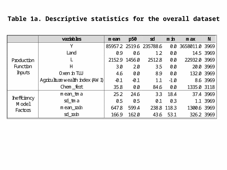
Table 1a. Descriptive statistics for the overall dataset

variables mean p50 sd min max N

Production Function

Inputs

Y 85957.2 2519.6 235788.6 0.0 3658011.0 3969 Land 0.9 0.6 1.2 0.0 14.5 3969

L 2152.9 1456.0 2512.8 0.0 22932.0 3969 H 3.0 2.0 3.5 0.0 20.0 3969

Oxen in TLU 4.6 0.0 8.9 0.0 132.0 3969 Agriculture wealth index (AWI) -0.1 -0.1 1.1 -1.0 8.6 3969

Chem_fert 35.8 0.0 84.6 0.0 1335.0 3118

Ineffciency Model Factors

mean_tma 25.2 24.6 3.3 18.4 37.4 3969 sd_tma 0.5 0.5 0.1 0.3 1.1 3969

mean_rain 647.8 599.4 238.8 118.3 1300.6 3969 sd_rain 166.9 162.0 43.6 53.1 326.2 3969

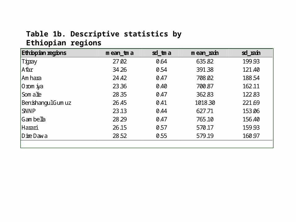
Table 1b. Descriptive statistics by Ethiopian regions

Ethiopian regions mean_tma sd_tma mean_rain sd_rain Tigray 27.02 0.64 635.82 199.93 Afar 34.26 0.54 391.38 121.40 Amhara 24.42 0.47 708.02 188.54 Oromiya 23.36 0.40 700.87 162.11 Somalie 28.35 0.47 362.83 122.83 Benishangul Gumuz 26.45 0.41 1018.30 221.69 SNNP 23.13 0.44 627.71 153.06 Gambella 28.29 0.47 765.10 156.40 Harari 26.15 0.57 570.17 159.93 Dire Dawa 28.52 0.55 579.19 160.97

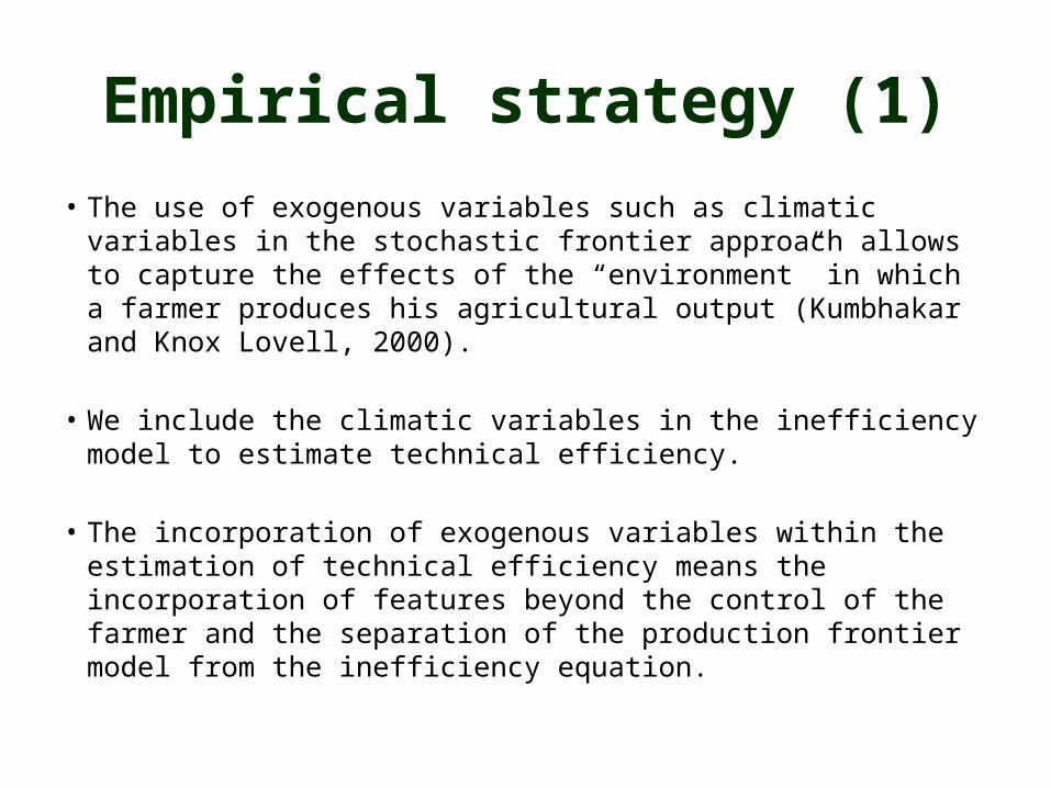
Empirical strategy (1)• The use of exogenous variables such as climatic variables in the

stochastic frontier approach allows to capture the effects of the “environment” in which a farmer produces his agricultural output (Kumbhakar and Knox Lovell, 2000).

• We include the climatic variables in the inefficiency model to estimate technical efficiency.

• The incorporation of exogenous variables within the estimation of technical efficiency means the incorporation of features beyond the control of the farmer and the separation of the production frontier model from the inefficiency equation.

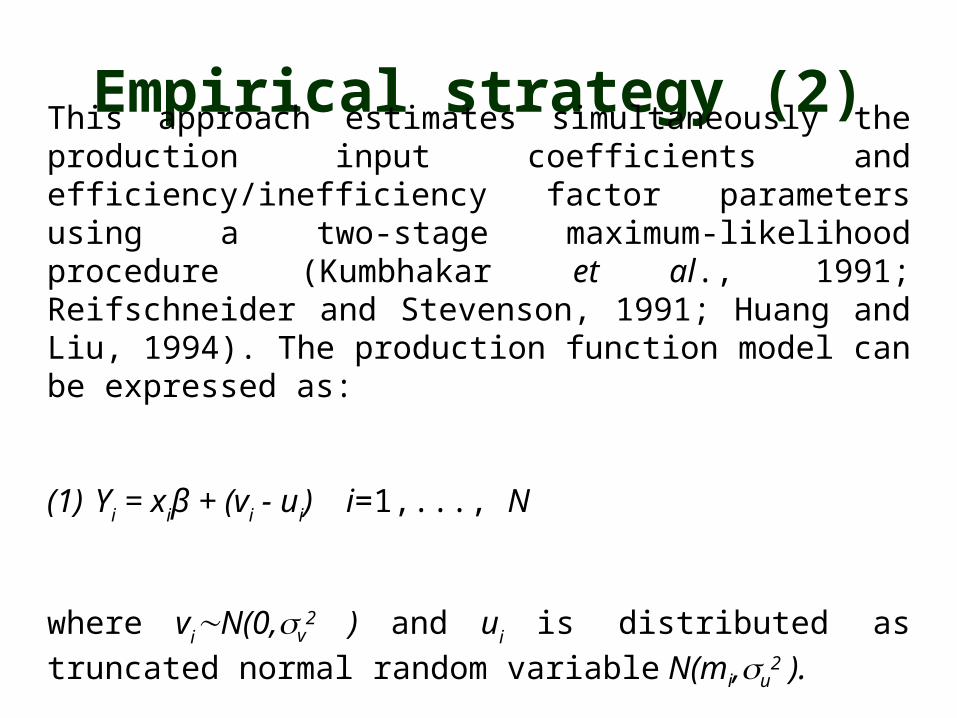
Empirical strategy (2)This approach estimates simultaneously the production input coefficients and efficiency/inefficiency factor parameters using a two-stage maximum-likelihood procedure (Kumbhakar et al., 1991; Reifschneider and Stevenson, 1991; Huang and Liu, 1994). The production function model can be expressed as:

(1) Yi = xiβ + (vi - ui) i=1,..., N

where viN(0,v2 ) and ui is distributed as truncated normal random

variable N(mi,u2 ).

Empirical strategy (3)The mean of this truncated normal distribution is a function of systematic variables that can influence the efficiency of a farmer:

(2) mi = zi + εi

where zi is a px1 vector of variables that may have an indirect effect on the production function of an Ethiopian household; is a 1xp vector of parameters to be estimated and εi is defined by the truncation of the normal distribution with zero mean and variance 2

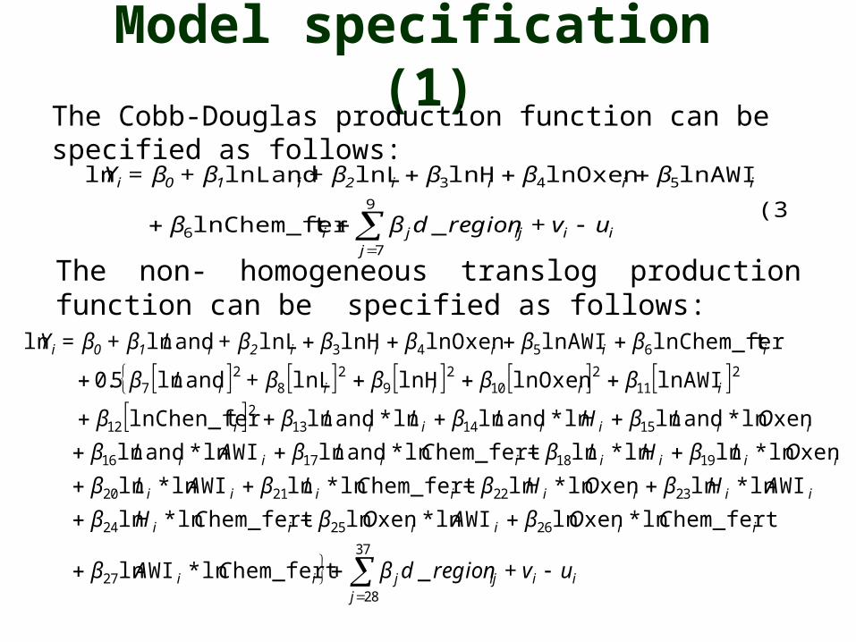
Model specification (1)The Cobb-Douglas production function can be specified as follows:

(3)_tlnChem_fer

lnAWIlnOxenlnHlnLlnLandln9

76

543

iij

ijji

iiii2i10i

uv+regiondββ

ββββ+β+β=Y

The non- homogeneous translog production function can be specified as follows:

iij

ijjii

iiiiii

iiiiiiii

iiiiiiii

iiiiiii

iiiii

iiiii2i10i

uv+regiondβCAβ

COβAOβCHβ

AHβOHβCLβALβ

OLβHLβCLβALβ

OLβHLβLLββ

ββββ+Lβ

βββββ+Lβ+β=Y

37

2827

262524

23222120

19181716

1514132

12

211

210

29

28

27

6543

_hem_fertln*WIln

hem_fertln*xenlnWIln*xenlnhem_fertln*ln

WIln*lnxenln*lnhem_fertln*lnWIln*ln

xenln*lnln*lnhem_fertln*andlnWIln*andln

xenln*andlnln*andlnln*andlntlnChen_fer

lnAWIlnOxenlnHlnLandln5.0

tlnChem_ferlnAWIlnOxenlnHlnLandlnln

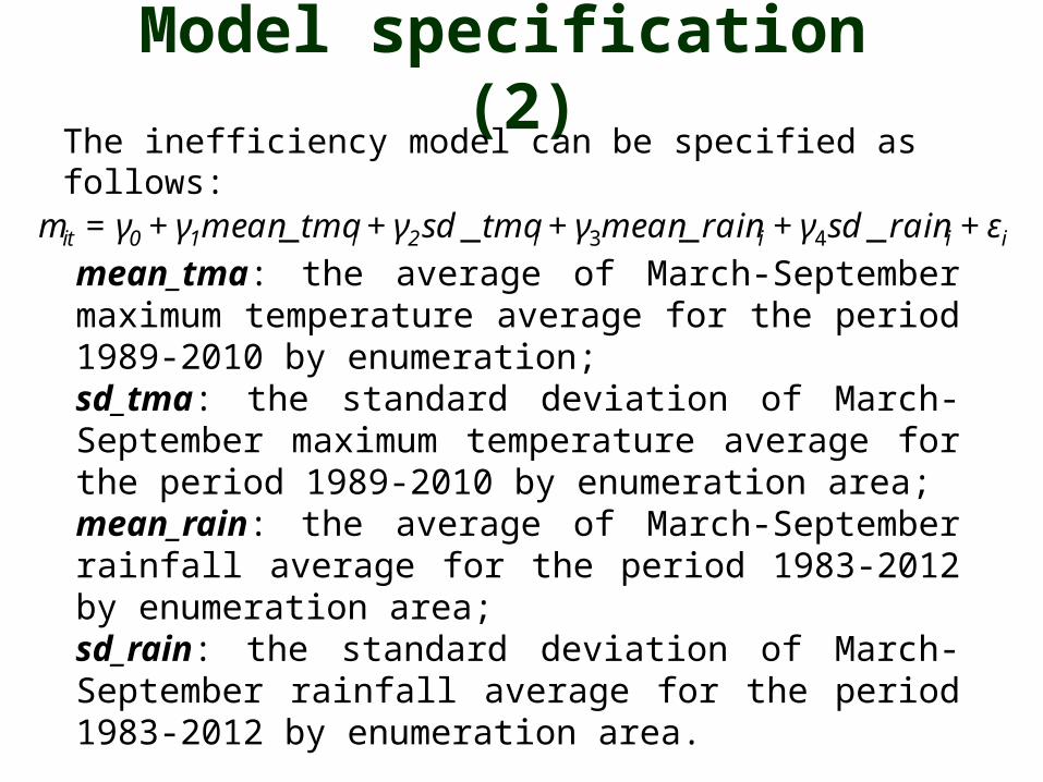
Model specification (2)The inefficiency model can be specified as follows:

mean_tma: the average of March-September maximum temperature average for the period 1989-2010 by enumeration; sd_tma: the standard deviation of March-September maximum temperature average for the period 1989-2010 by enumeration area; mean_rain: the average of March-September rainfall average for the period 1983-2012 by enumeration area;sd_rain: the standard deviation of March-September rainfall average for the period 1983-2012 by enumeration area.

iiii2i10it ε+rainsdγ+rainmeanγ+tmasdγ+tmameanγ+γ=m ____ 43

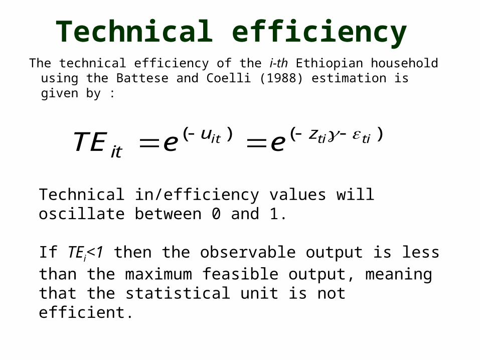
Technical efficiency The technical efficiency of the i-th Ethiopian household using

the Battese and Coelli (1988) estimation is given by :

)()( titiit zuit eeTE

Technical in/efficiency values will oscillate between 0 and 1.

If TEi<1 then the observable output is less than the maximum feasible output, meaning that the statistical unit is not efficient.

Table 3. Tests for functional form of the production function

Model 1 H0 restricted model H1 unrestricted model Restrictions LR test P value Decision Homo. Translog Non-homo. Translog 6 1933.93 0.00 Reject H0 C-D homo Non-homo. Translog 21 5.41 0.99 Do not reject H0 C-D homo Homo. Translog 15 -1939.3 0.99 Do not reject H0

Model 2 H0 restricted model H1 unrestricted model Restrictions LR test P value Decision Homo. Translog Non-homo. Translog 7 16.12 0.02 Reject H0 C-D homo Non-homo. Translog 21 119.31 0.00 Reject H0 C-D homo Homo. Translog 14 103.19 0.00 Reject H0 Notes: H0 is the null hypothesis, H1 the alternative. Tests were conducted at the 5% level.

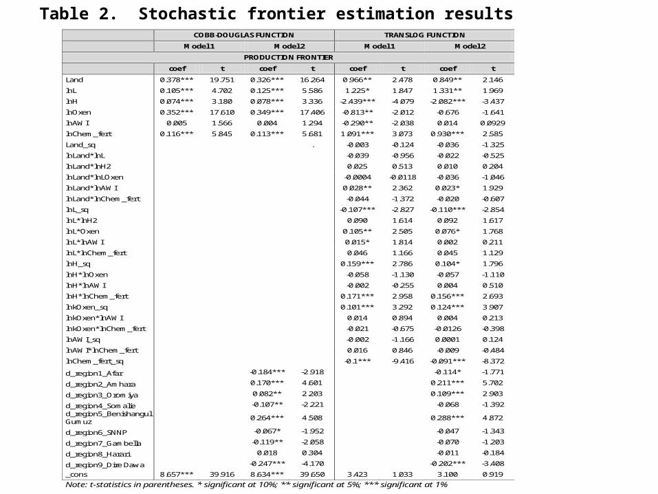
Table 2. Stochastic frontier estimation results

COBB-DOUGLAS FUNCTION TRANSLOG FUNCTION

Model 1 Model 2 Model 1 Model 2

PRODUCTION FRONTIER

coef t coef t coef t coef t

Land 0.378*** 19.751 0.326*** 16.264 0.966** 2.478 0.849** 2.146

lnL 0.105*** 4.702 0.125*** 5.586 1.225* 1.847 1.331** 1.969

lnH 0.074*** 3.180 0.078*** 3.336 -2.439*** -4.079 -2.082*** -3.437

lnOxen 0.352*** 17.610 0.349*** 17.406 -0.813** -2.012 -0.676 -1.641

lnAWI 0.005 1.566 0.004 1.294 -0.290** -2.038 0.014 0.0929

lnChem_fert 0.116*** 5.845 0.113*** 5.681 1.091*** 3.073 0.930*** 2.585

Land_sq . -0.003 -0.124 -0.036 -1.325

lnLand*lnL -0.039 -0.956 -0.022 -0.525

lnLand*lnH2 0.025 0.513 0.010 0.204

lnLand*lnLOxen -0.0004 -0.0118 -0.036 -1.046

lnLand*lnAWI 0.028** 2.362 0.023* 1.929

lnLand*lnChem_fert -0.044 -1.372 -0.020 -0.607

lnL_sq -0.107*** -2.827 -0.110*** -2.854

lnL*lnH2 0.090 1.614 0.092 1.617

lnL*Oxen 0.105** 2.505 0.076* 1.768

lnL*lnAWI 0.015* 1.814 0.002 0.211

lnL*lnChem_fert 0.046 1.166 0.045 1.129

lnH_sq 0.159*** 2.786 0.104* 1.796

lnH*lnOxen -0.058 -1.130 -0.057 -1.110

lnH*lnAWI -0.002 -0.255 0.004 0.510

lnH*lnChem_fert 0.171*** 2.958 0.156*** 2.693

lnkOxen_sq 0.101*** 3.292 0.124*** 3.907

lnkOxen*lnAWI 0.014 0.894 0.004 0.213

lnkOxen*lnChem_fert -0.021 -0.675 -0.0126 -0.398

lnAWI_sq -0.002 -1.166 0.0001 0.124

lnAWI*lnChem_fert 0.016 0.846 -0.009 -0.484

lnChem_fert_sq -0.1*** -9.416 -0.091*** -8.372

d_region1_Afar -0.184*** -2.918 -0.114* -1.771

d_region2_Amhara 0.170*** 4.601 0.211*** 5.702

d_region3_Oromiya 0.082** 2.203 0.109*** 2.903

d_region4_Somalie -0.107** -2.221 -0.068 -1.392 d_region5_Benishangul Gumuz 0.264*** 4.508 0.288*** 4.872

d_region6_SNNP -0.067* -1.952 -0.047 -1.343

d_region7_Gambella -0.119** -2.058 -0.070 -1.203

d_region8_Harari 0.018 0.304 -0.011 -0.184

d_region9_Dire Dawa -0.247*** -4.170 -0.202*** -3.408

_cons 8.657*** 39.916 8.634*** 39.650 3.423 1.033 3.100 0.919

Note: t-statistics in parentheses. * significant at 10%; ** significant at 5%; *** significant at 1%

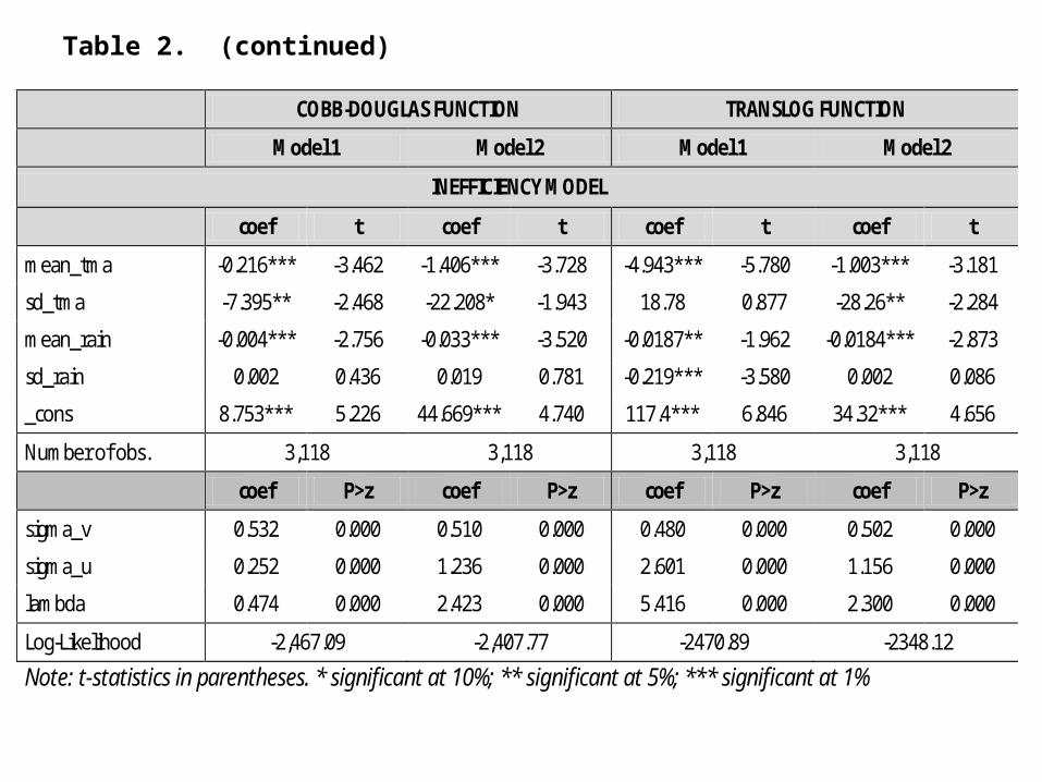
Table 2. (continued)

COBB-DOUGLAS FUNCTION TRANSLOG FUNCTION

Model 1 Model 2 Model 1 Model 2

INEFFICIENCY MODEL

coef t coef t coef t coef t

mean_tma -0.216*** -3.462 -1.406*** -3.728 -4.943*** -5.780 -1.003*** -3.181

sd_tma -7.395** -2.468 -22.208* -1.943 18.78 0.877 -28.26** -2.284

mean_rain -0.004*** -2.756 -0.033*** -3.520 -0.0187** -1.962 -0.0184*** -2.873

sd_rain 0.002 0.436 0.019 0.781 -0.219*** -3.580 0.002 0.086

_cons 8.753*** 5.226 44.669*** 4.740 117.4*** 6.846 34.32*** 4.656

Number of obs. 3,118 3,118 3,118 3,118

coef P>z coef P>z coef P>z coef P>z

sigma_v 0.532 0.000 0.510 0.000 0.480 0.000 0.502 0.000

sigma_u 0.252 0.000 1.236 0.000 2.601 0.000 1.156 0.000

lambda 0.474 0.000 2.423 0.000 5.416 0.000 2.300 0.000

Log-Likelihood -2,467.09 -2,407.77 -2470.89 -2348.12

Note: t-statistics in parentheses. * significant at 10%; ** significant at 5%; *** significant at 1%

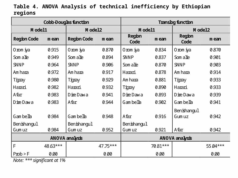
Table 4. ANOVA Analysis of technical inefficiency by Ethiopian regions

Cobb-Douglas function Translog function

Model 1 Model 2 Model 1 Model 2

Region Code mean Region Code mean Region Code

mean Region Code

mean

Oromiya 0.915 Oromiya 0.870 Oromiya 0.834 Oromiya 0.870

Somalie 0.949 Somalie 0.894 SNNP 0.837 Somalie 0.901

SNNP 0.964 SNNP 0.906 Somalie 0.870 SNNP 0.903

Amhara 0.972 Amhara 0.917 Harari 0.878 Amhara 0.914

Tigray 0.980 Tigray 0.929 Amhara 0.881 Tigray 0.933

Harari 0.982 Harari 0.932 Tigray 0.890 Harari 0.933

Afar 0.983 Dire Dawa 0.941 Dire Dawa 0.893 Dire Dawa 0.939

Dire Dawa 0.983 Afar 0.944 Gambella 0.902 Gambella 0.941

Gambella 0.984 Gambella 0.948 Afar 0.916 Benishangul Gumuz 0.942

Benishangul Gumuz 0.984

Benishangul Gumuz 0.952

Benishangul Gumuz 0.921 Afar 0.942

ANOVA analysis ANOVA analysis

F 48.63***

47.75*** 70.81***

55.04***

Prob > F 0.00 0.00 0.00 0.00 Note: *** significant at 1%

Conclusion (1)This paper contributes to the climate change literature:

• by using a novel data set that combines information coming from two large-scale household surveys with geo-referenced historical rainfall and temperature data;

• by estimating the technical efficiency of Ethiopian households in the period 2011-12;

• by analysing the climate change effects on farmers’ efficiency taking into account the heterogeneity of climate areas (desert, tropical forest and plateau);

• by ranking the Ethiopian regions from the less efficient to the most efficient.

Conclusion (2)

• The results of the production functions are generally conform to our expectations and to literature;

• In the inefficiency model, we find that long term climatic variables computed on precipitations and maximum temperatures in the cropping season affect positively farmers’ efficiency;

• Regions in the east side of the country (suc as Somalie and Oromiya) are less efficient than regions in the west side (such as Benishangul Gumuz or Gambella).

Further developments

• We calculated a series of intra- and inter-seasonal indicators to measure both the level and variability of rainfall and maximum temperature:

• intra-seasonal indicators measure weather fluctuations such as Walsh and Lawler (1981) Seasonality Index for precipitations;

• inter-seasonal indicators measure the climate of a specific area such as Coefficient of Variation computed for the past 10, 5 and 3 years.