clientelistic politics and pro-poor targeting: rules

Clientelistic Politics and Pro-Poor Targeting:Rules versus Discretionary Budgets∗

Dilip Mookherjee†, and Anusha Nath‡

October 5, 2020

Abstract

Past research has shown evidence of clientelistic politics in delivery of benefits and

manipulation of local government program budgets by upper level officials in the context

of West Bengal, India. We examine the implications of moving to a system of formula

based program budgets on pro-poor targeting. Using a household panel data for 2004-

2008, we show that targeting of anti-poverty programs within local governments (GPs)

was progressive. We estimate the effect of replacing observed GP program budgets by

those implied by a rule-based formula recommended by the 3rd State Finance Commis-

sion (SFC) based on GP demographic characteristics. We find that the SFC formula

would have reduced pro-poor targeting of anti-poverty programs. Moreover, alternative

formulae obtained by varying weights on GP characteristics used in the SFC formula

improve targeting only marginally. Hence clientelism has been successful in targeting

benefits to the poor, and there is little additional scope for improvements from transition-

ing to formula-based budgeting.

JEL Classification: H40, H75, H76, O10, P48.

∗Prepared for a WIDER conference on Clientelistic Politics and Development. For financial support, wethank the EDI network, IGC and WIDER. The views expressed herein are those of the authors and not neces-sarily those of the Federal Reserve Bank of Minneapolis or the Federal Reserve System.†Boston University. email: [email protected]‡Federal Reserve Bank of Minneapolis. email: [email protected]

1

1 Introduction

A lot of recent research has provided evidence of political clientelism in the delivery of

benefits by West Bengal local governments (Bardhan et al (2010, 2015, 2020), Bardhan-

Mookherjee (2012), Dey and Sen (2016), Shenoy and Zimmerman (2020)). Bardhan et al

(2020) show that plausibly exogenous variation in delivery of excludable private benefits,

especially of a recurring nature such as public works employment, to households between

2009-11 induced their heads to shift expressed support to the political party controlling the

incumbent local government (GP). At the same time, household political support did not re-

spond to the delivery of non-excludable local public goods that they reported benefitting from.

Moreover, middle tiers of government at the district and block level manipulated program

budgets of GPs in their jurisdiction for private benefits in response to exogenous changes in

political competition.1 GPs controlled by the same party at both tiers received higher budgets,

while those controlled by rival parties experienced severe cuts. Parallel to the pattern of voter

responsiveness at the household level, these manipulations were restricted only to excludable

private benefit programs. Dey and Sen (2016) and Shenoy and Zimmerman (2020) examine

post-2011 data and use regression discontinuity based causal evidence that winners of close

election races raised employment program scales in aligned GPs, presumably manifesting

rewards to GP leaders who helped deliver votes for their party.

Evidently discretionary control over benefit distribution is exercised opportunistically,

both within and across GPs. This raises the question: could targeting be improved by switch-

ing to a formula-bound programmatic system of transfers which would remove scope for such

discretion? Assessing the extent of such improvements requires estimating the effects of a

counterfactual policy reform, and comparing them to observed allocations.

The extent of such improvement would likely depend on the information base available

for the design of a formula. If program designers had perfect information about the distribu-

tion of socio-economic status (SES) across households, and could costlessly deliver benefits

directly to households, perfect targeting could be achieved. In practice, upper level govern-

ments (ULGs) at the national or state level neither have such information, and frequently

lack the capacity to transfer benefits directly to households. This is particularly the case

in India, where the level of disaggregation of governments information regarding economic

backwardness is limited to village census records and household sample surveys representa-

1The causal effect of changing political competition was identified by comparing changes in budgets ofGPs redistricted in 2007 to more contested state assembly constituencies, with others not redistricted or thoseredistricted to less contested constituencies.

2

tive at best at the district level. A large fraction of the rural poor do not have functioning bank

accounts. Even the biometric citizen identification Aadhar cards that have been rolled out

nationwide over the past decade are yet to have universal coverage, cannot be integrated with

bank accounts, and contain many errors.2 Hence GPs have traditionally been delegated the

task of identifying SES status of households within their jurisdiction, selecting beneficiaries

and delivering various benefit (mostly in-kind) programs. Middle level governments (MLGs

hereafter) at block and district levels have been delegated responsibility of allocating program

budgets across GPs within their jurisdiction, based on their knowledge of the distribution of

poverty and need across GPs. While the weaknesses in informational and delivery capacity of

ULGs continue to persist, a formula-bound program would have to continue to devolve intra-

village allocation powers to GPs. Hence the scope of programmatic policy reforms would

be limited to the system by which GP program budgets are determined. Middle level gov-

ernments (MLGs hereafter) at block and district levels would no longer exercise discretion

over GP budgets, once they are replaced by formulae based on ‘hard’ information available

to ULGs. A recent World Bank program for strengthening local governance in West Bengal

involving 1000 GPs has been based on direct grants to GPs based on transparent formulae,

constitutes an example of such an approach.3

However, imperfections in information about distribution of poverty across villages on

which formula bound GP budgets would be based, would also lead to less than perfect target-

ing. There would be errors both of inclusion (prosperous villages with few poor households

that are misclassified as poor villages would end up receiving large budgets) and of exclusion

(poor villages misclassified as prosperous failing to qualify for program grants). It is a priori

unclear whether the formula bound program would generate better pro-poor targeting com-

pared to the existing discretionary system. The net result would depend on (a) the superiority

of ‘local soft’ information available to MLGs relative to the ‘hard’ information available to

ULGs regarding the distribution of poverty across GP areas, and (b) the nature of incentives

for MLGs generated by political clientelism to target benefits towards truly poor areas. The

latter in turn depends partly on whether elections in poorer regions are less contested, and

on patterns of political alignment between MLGs and ULGs. Also relevant is the relative

responsiveness of votes of the poor and non-poor to benefit delivery. Some have argued that

clientelism creates a bias in favor of distributing benefits towards the poor, since their votes

are cheaper to ‘buy’. Others have argued that the poor vote is determined more by ‘identity’

2For recent discussion of these problems, see Dreze, Khera and Somanchi (2020).3See for instance https://projects.worldbank.org/en/projects-operations/project-detail/P159427.

3

considerations and less by actual governance performance, while non-poor and better edu-

cated voters are more prone to swing based on benefits received. A priori, it is hard to predict

whether political opportunism for MLGs in a clientelistic setting would translate into a pro-

or anti-poor bias.

Hence the effect of moving to formula based GP budgets can only be assessed empirically.

This is the question we address in this paper. Using household panel surveys in a sample of

59 GPs covering 2400 households over a five year period 2004-08, we start by studying

targeting patterns in the intra-village distribution of benefits by GPs across households of

varying SES within their jurisdiction. The household surveys include demographic, asset and

income information, allowing us to classify them into categories of ultra-poor, moderately

poor and marginally poor. Our definition of these categories is based on whether three, two

or one criteria are satisfied by any given household: if it is landless (owns no agricultural

land), if the head is uneducated (zero years of schooling), and if the household belongs to a

scheduled caste or tribe (SC/ST). Besides capturing the multidimensionality of poverty, we

also verify that this method accurately measures the depth of poverty: the distribution of

annual reported income, the value of land owned, or of the reported value of the dwelling of

successive classes are ordered by first order stochastic dominance.

The intra-GP targeting pattern for anti-poverty programs (which conditions on the bud-

get the GP receives from MLGs) reveals a clear bias in favor of poor households. Poorer

households were more likely to receive either an employment benefit, or any of the other

anti-poverty benefits (low income housing and sanitation, below-poverty-line (BPL) cards

entitling holders to subsidized grains and fuel, subsidized loans). On the other hand, the allo-

cation of subsidized farm inputs was negatively correlated with landlessness and household

poverty status. For all programs, increased GP program budgets (proxied by per household

benefits distributed in the GP) resulted in near-uniform increases in allocations to all house-

holds irrespective of poverty status. The targeting patterns are robust to varying specifications,

either of functional form, controls for village characteristics or inclusion of year, GP or dis-

trict dummies. These results are also unchanged in an instrumental variable (IV) regression

where we instrument for the per household GP benefit by the corresponding per household

GP benefit in all others GPs in the same district (a la Levitt-Snyder (1997)). The fact that

conditional on GP budgets the targeting patterns are unaffected by replacing GP dummies

by district dummies is consistent with the hypothesis that GP budgets represent the primary

channel by which targeting is manipulated by MLGs. And the robustness of targeting patterns

with respect to the potential endogeneity of GP budgets indicates that the estimated impact

4

of GP budgets can be interpreted causally. Therefore we can use them to predict the targeting

impacts of changing the way GP budgets are set.

Next we examine how observed GP budgets varied across GPs. These were also pro-

gressive: GPs with a higher household proportion of ultra or moderately poor households

were allocated higher budgets. We compare the observedobserved budgets with those which

would have resulted in reallocating district budgets across GPs using a formula for alloca-

tion of fiscal grants to GPs recommended by the 3rd State Finance Commission (SFC) of the

state of West Bengal. The SFC formula incorporates six village characteristics from the Cen-

sus and some household surveys: population size, SC/ST proportion, proportion of female

illiterates, a food insecurity index, proportion of agricultural workers, village infrastructure

and population density. The SFC recommended grants turn out to be less progressive than

the allocations actually observed. We show this in two different ways. First, across GPs,

recommended grants were less positively correlated with the village proportion of (at least

moderately) poor households. Second, we use the intra-GP targeting pattern to estimate how

the the expected number of benefits would have changed for any given household in the

sample. We aggregate this to estimate the resulting variation in the expected number and

state-wide share of benefits accruing to different poverty groups. In terms of the expected

number of benefits, the formula-bound system would have unambiguously led to a decline

in allocation of anti-poverty programs to poor groups, while the distribution of farm subsidy

programs would have remained unaffected. The same is true for the benefit shares of the ultra

and moderately poor groups combined.

Finally, we examine whether variations on the weights used in the SFC formula could

have improved targeting beyond the observed allocations. For employment benefits, the share

of the ultra-poor could at best have been increased from 16 to 17%, but only at the cost of

reducing the share of the moderately poor by almost the same magnitude. Only in the case of

non-employment anti-poverty benefits it would have been possible to raise shares of both the

ultra-poor and moderately poor, and the expected number of benefits for either group (from

.10 to .13 for the ultra-poor and from .06 to .07 for the moderately poor, both increases being

statistically significant). However, the magnitude of this improvement is modest at best.

Based on these results, we are inclined to infer that clientelism as it operated in rural West

Bengal did not seriously distort pro-poor targeting. The scope for further improvements by

switching to formula based GP budgets is limited. This indicates the importance of improving

the information available to ULGs regarding ownership of key assets of land and education

at the household level, to eventually enable transition to a system of direct cash transfers

5

to households rather than GPs. In the interim when information remains poor and financial

inclusion of the poor is still incomplete, there seems to be little scope for improving targeting

of existing in-kind anti-poverty programs.

Our work relates to some recent literature studying the implications of moving from dis-

cretionary to formula based program grants in Brazil by Azulai (2017) and Finan and Maz-

zocco (2020), and in drought relief declarations in south Indian states (Tarquinio (2020)).

It is evident from this emerging literature that the expected results vary considerably across

different contexts and countries.

Section 2 provides details of the setting and describes the data. Section 3 then presents

evidence on intra-GP targeting patterns, which is used in Section 4 to estimate the impacts of

switching to formula based GP budgets. Section 5 concludes with lessons for policy reforms,

and fruitful directions of future investigation.

2 Context, Data and Descriptive Statistics

Each Indian state has a hierarchy of local governments (panchayats) in rural areas that deliver

diverse in-kind benefits to households living in villages. Most of these programs are financed

by central and state governments. District-level governments, zilla parishads (ZPs), allocate

funds to middle-tier governments at the ‘block’ level, which comprise an elected body pan-

chayat samiti (PS) and appointed bureaucrats in the Block Development Offices. The middle

tier then allocates funds to bottom-tier gram panchayats (GPs) within their block, who in turn

distribute benefits across and within villages in their jurisdiction. Each GP oversees 10-15

villages, and each village in turn includes an average of 300 households. GPs also admin-

ister rural infrastructure projects, in which they employ the local population. Despite being

subject to oversight both below (from village assembly meetings) and above (middle level

governments that approve projects, expenditures and audit accounts), GPs exercise consider-

able discretion in their allocation and project decisions. MLG officials face considerably less

scrutiny, as there are no stated criteria for horizontal allocation of funds or project approvals

across GPs reporting to them. The near-complete absence of any transparency in inter-GP

allocations allows MLG officials with great latitude to manipulate them.

Our data on benefits received by households comes from a household survey carried out

in 2011 in 89 villages in 57 GPs spread through all 18 agricultural districts of West Bengal

in 2011, and has been used in previous papers (Bardhan et al (2020)). There are over 2400

households in the sample, amounting to approximately 25 households per village. House-

6

holds within a village were selected by sampling randomly in different land strata. Table 1

provides a summary of the demographic characteristics of these households. Over half own

no agricultural land, nearly one in three are SC/ST, and one-third household heads are unedu-

cated. Agricultural cultivation is the primary occupation among the landed, while the landless

are primarily workers relying on labor earnings.

Table 1: Summary Statistics: Demographics

Agri Land No. of Characteristics of Head of HouseholdsOwned(acres)

Households Avg.Age

% Males Years ofSchooling

%SC/ST

% inAgriculture

Landless 1214 45 88 6.6 37.4 260-1.5 658 48 88 7.8 38.9 65

1.5-2.5 95 56 92 10.8 22.4 822.5-5 258 58 93 11.1 27.1 725-10 148 60 89 12.5 26.1 66> 10 29 59 100 13.9 30.9 72All 2402 49 89 8.0 35.4 47

Note. This table provides demographic characteristics of the head of households (who were the main respon-dents to the survey) in 2004. % Agriculture refers to percentage of household heads whose primary occupationis agriculture.

We focus on the 2004-08 period partly because it corresponded to the five years of a sin-

gle GP administration, which came into power following an election in the middle of 2003.

Moreover, this corresponds to the period studied in Bardhan et al (2020) where GP budgets

for private benefits were shown to have been politically manipulated by ULGs based on polit-

ical competition and alignment. Since our focus is on political clientelism, we focus attention

on excludable private benefit programs. The most important of these is employment in lo-

cal infrastructure construction programs managed by the GP, such as Jawahar Rozgar Yojana

(JRY), National Rural Employment Guarantee Act (NREGA) and Member of Parliament Lo-

cal Area Development Scheme (MPLADS). These employment programs employed roughly

5-6% of the local population in each year between 2004-08. Mostly carried out in the lean

agricultural season between March and July, they provide employed households the opportu-

nity to earn a wage set statutorily above the average market wage rate. In years of low rainfall

when private employment opportunities and wages are low, they are an important source of in-

come protection for poor households. Other anti-poverty programs include subsidized loans,

housing/toilet construction subsidies, Below Poverty Line (BPL) cards which identify poor

7

households and entitle them to subsidized food grains and other household items. GPs also

help distribute agricultural minikits that contain subsidized seeds, fertilizers and pesticides,

but this is an agricultural development program rather than an antipoverty program. We will

see the targeting patterns for these minikits differ substantially from all the other programs.

During 2004-08 between 9-10% of households received at least one kind of private benefit

from the GP in any given year; over the entire five year period approximately three out of five

households received at least one benefit.

Our data includes different dimensions of low socio-economic status (SES): whether a

household belongs to an SC or ST, whether it is landless, and whether head of household is un-

educated. We classify households into four groups: ultra-poor, moderately poor, marginally

poor and non-poor depending on whether all, two, one or none of these conditions apply. This

is a measure of the number of dimensions on which a household is poor. It also corresponds

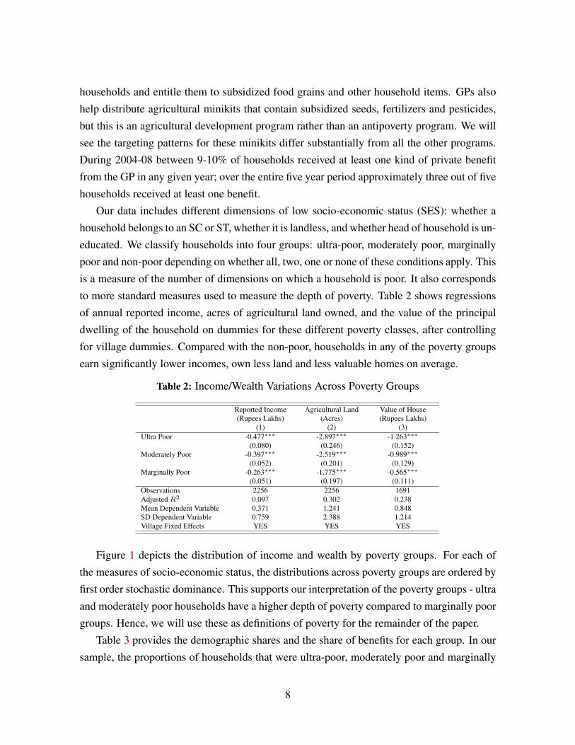
to more standard measures used to measure the depth of poverty. Table 2 shows regressions

of annual reported income, acres of agricultural land owned, and the value of the principal

dwelling of the household on dummies for these different poverty classes, after controlling

for village dummies. Compared with the non-poor, households in any of the poverty groups

earn significantly lower incomes, own less land and less valuable homes on average.

Table 2: Income/Wealth Variations Across Poverty Groups

Reported Income Agricultural Land Value of House(Rupees Lakhs) (Acres) (Rupees Lakhs)

(1) (2) (3)Ultra Poor -0.477∗∗∗ -2.897∗∗∗ -1.263∗∗∗

(0.080) (0.246) (0.152)Moderately Poor -0.397∗∗∗ -2.519∗∗∗ -0.989∗∗∗

(0.052) (0.201) (0.129)Marginally Poor -0.263∗∗∗ -1.775∗∗∗ -0.565∗∗∗

(0.051) (0.197) (0.111)Observations 2256 2256 1691Adjusted R2 0.097 0.302 0.238Mean Dependent Variable 0.371 1.241 0.848SD Dependent Variable 0.759 2.388 1.214Village Fixed Effects YES YES YES

Figure 1 depicts the distribution of income and wealth by poverty groups. For each of

the measures of socio-economic status, the distributions across poverty groups are ordered by

first order stochastic dominance. This supports our interpretation of the poverty groups - ultra

and moderately poor households have a higher depth of poverty compared to marginally poor

groups. Hence, we will use these as definitions of poverty for the remainder of the paper.

Table 3 provides the demographic shares and the share of benefits for each group. In our

sample, the proportions of households that were ultra-poor, moderately poor and marginally

8

Figure 1: Distribution of Income and Wealth by Poverty Groups

0

.2

.4

.6

.8

1

Cum

ulat

ive

Prob

abilit

y

0 .5 1 1.5 2 2.5Total Income in 2004 (Rupees Lakhs)

c.d.f. of marginal c.d.f. of moderate c.d.f. of notpoor c.d.f. of ultra

0

.2

.4

.6

.8

1

Cum

ulat

ive

Prob

abilit

y

0 2 4 6 8 10Total Agricultural Landholdings in 2004 (Acres)


0

.2

.4

.6

.8

1

Cum

ulat

ive

Prob

abilit

y

0 2 4 6 8Value of House (Rupees Lakhs)


poor was 8.5%, 27.5% and 38.3% respectively. The share of employment and non-employment

anti-poverty benefits for ultra and moderately poor households is higher than their demo-

graphic shares. However, the opposite is the case for farm subsidies.

Table 3: Poverty Groups: Demographic Share and Share of Reported Benefits

Group Demographic Share of Reported BenefitsShare Employment Anti-poverty Farm Subsidy

Ultra Poor 8.53 17.38 14.30 1.59Moderately Poor 27.56 35.36 34.98 12.70Marginally Poor 38.33 32.39 31.85 42.33Non-poor 25.58 14.86 18.87 43.39

3 Within-GP Targeting Patterns

In this section we examine targeting patterns within GPs. Table 3 presents a Poisson count

regression for the number of benefits received by a household in any given year; the reported

coefficients can be interpreted as the change in log of the expected number of benefits asso-

ciated with a unit change in each regressor. The regressors include the household’s poverty

9

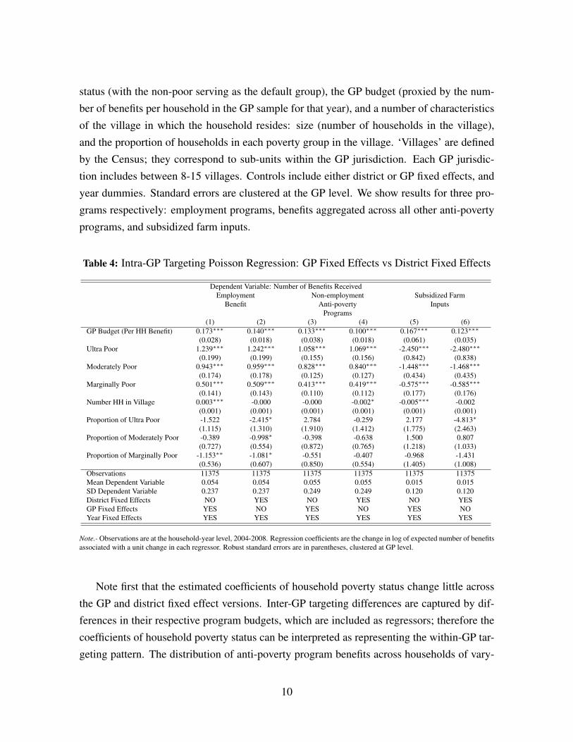
status (with the non-poor serving as the default group), the GP budget (proxied by the num-

ber of benefits per household in the GP sample for that year), and a number of characteristics

of the village in which the household resides: size (number of households in the village),

and the proportion of households in each poverty group in the village. ‘Villages’ are defined

by the Census; they correspond to sub-units within the GP jurisdiction. Each GP jurisdic-

tion includes between 8-15 villages. Controls include either district or GP fixed effects, and

year dummies. Standard errors are clustered at the GP level. We show results for three pro-

grams respectively: employment programs, benefits aggregated across all other anti-poverty

programs, and subsidized farm inputs.

Table 4: Intra-GP Targeting Poisson Regression: GP Fixed Effects vs District Fixed Effects

Dependent Variable: Number of Benefits ReceivedEmployment Non-employment Subsidized Farm

Benefit Anti-poverty InputsPrograms

(1) (2) (3) (4) (5) (6)GP Budget (Per HH Benefit) 0.173∗∗∗ 0.140∗∗∗ 0.133∗∗∗ 0.100∗∗∗ 0.167∗∗∗ 0.123∗∗∗

(0.028) (0.018) (0.038) (0.018) (0.061) (0.035)Ultra Poor 1.239∗∗∗ 1.242∗∗∗ 1.058∗∗∗ 1.069∗∗∗ -2.450∗∗∗ -2.480∗∗∗

(0.199) (0.199) (0.155) (0.156) (0.842) (0.838)Moderately Poor 0.943∗∗∗ 0.959∗∗∗ 0.828∗∗∗ 0.840∗∗∗ -1.448∗∗∗ -1.468∗∗∗

(0.174) (0.178) (0.125) (0.127) (0.434) (0.435)Marginally Poor 0.501∗∗∗ 0.509∗∗∗ 0.413∗∗∗ 0.419∗∗∗ -0.575∗∗∗ -0.585∗∗∗

(0.141) (0.143) (0.110) (0.112) (0.177) (0.176)Number HH in Village 0.003∗∗∗ -0.000 -0.000 -0.002∗ -0.005∗∗∗ -0.002

(0.001) (0.001) (0.001) (0.001) (0.001) (0.001)Proportion of Ultra Poor -1.522 -2.415∗ 2.784 -0.259 2.177 -4.813∗

(1.115) (1.310) (1.910) (1.412) (1.775) (2.463)Proportion of Moderately Poor -0.389 -0.998∗ -0.398 -0.638 1.500 0.807

(0.727) (0.554) (0.872) (0.765) (1.218) (1.033)Proportion of Marginally Poor -1.153∗∗ -1.081∗ -0.551 -0.407 -0.968 -1.431

(0.536) (0.607) (0.850) (0.554) (1.405) (1.008)Observations 11375 11375 11375 11375 11375 11375Mean Dependent Variable 0.054 0.054 0.055 0.055 0.015 0.015SD Dependent Variable 0.237 0.237 0.249 0.249 0.120 0.120District Fixed Effects NO YES NO YES NO YESGP Fixed Effects YES NO YES NO YES NOYear Fixed Effects YES YES YES YES YES YES

Note.- Observations are at the household-year level, 2004-2008. Regression coefficients are the change in log of expected number of benefitsassociated with a unit change in each regressor. Robust standard errors are in parentheses, clustered at GP level.

Note first that the estimated coefficients of household poverty status change little across

the GP and district fixed effect versions. Inter-GP targeting differences are captured by dif-

ferences in their respective program budgets, which are included as regressors; therefore the

coefficients of household poverty status can be interpreted as representing the within-GP tar-

geting pattern. The distribution of anti-poverty program benefits across households of vary-

10

ing SES within a GP is progressive: poorer households receive more benefits. The pattern is

exactly the opposite for subsidized farm inputs (driven mainly by a negative coefficient for

landless households). Hence GPs tends to distribute farm inputs quite differently — reflecting

either normative consideration of delivering benefits to those that would value them the most,

or landed elite appeasement/capture that may co-exist with clientelism (as argued in Bardhan

and Mookherjee (2012)).

A higher proportion of poor households residing in the village generally tends to lower

benefits received by a representative household, though these estimates tend to lack statistical

significance. These negative effects are more pronounced in the version with district rather

than GP fixed effects. Since the regression conditions on the GP program budget, it is likely to

arise mechanically from the GP budget constraint, combined with the progressive pattern of

targeting within the GP. Since poorer households are more likely to receive benefits than the

non-poor, a GP with a larger fraction of poor households and with a given budget will have

less available to distribute to non-poor households. It should not be interpreted as a form of

regressivity in the across-GP targeting pattern, which will be manifested in the allocation of

budgets across GPs (and will be studied in the next Section).

In order to simulate the intra-GP effects of changes in GP budgets, it is important to obtain

an unbiased estimate of the causal impact of changing these budgets. The preceding regres-

sion estimate of the GP budget effect is subject to various concerns. First, the GP budget is

not directly observed and is measured with error by its proxy, the per household benefit in the

sample. The resulting measurement error could result in a downward (attenuation) bias. Sec-

ond, the per capita benefit measure in the GP includes each household in the sample, thereby

mechanically inducing a positive bias. Third, GP budget allocations may not be exogenous as

they could be driven by political considerations of officials in upper level governments. To the

extent that these unobserved political considerations (competitive stakes, political alignment,

responsiveness of votes to program benefits) vary across GPs and are systematically corre-

lated with included village or household characteristics, the regression estimates in Table 3

may be biased.

To deal with these concerns, Table 4 presents an instrumental variable (IV) regression

where we instrument for the GP budget by average per household program scale in all otherGPs in the district. This is similar to the instrument used in earlier work of Levitt and Snyder

(1997) and Bardhan et al (2020). This reflects factors less likely to be correlated with GP-

specific unobserved political attributes, such as the scale of the program budget at the district

level (determined by financing constraints at the district level), and political attributes of other

11

GPs in the district with which the given GP is competing for funds. As explained in some

detail in Levitt and Snyder (1997) and Bardhan et al (2020), under plausible assumptions the

resulting IV estimate is likely to be less biased, with the bias tending to vanish as the number

of GPs per district becomes large.4

Owing to the incidental parameter problem, the IV regression excludes both year and GP

fixed effects. The first two columns for each kind of program (e.g., columns 1 and 2 for

employment benefits) show the effect of dropping these fixed effects in the non-IV version:

it lowers the coefficient of GP program scale somewhat, while leaving the coefficients of

household poverty status unchanged. The last two columns in each set (e.g., columns 2 and

3 for employment) compare the non-IV with the IV version, both without any fixed effects.

We see that the estimates of program scale and of household poverty status are practically

unchanged. Hence, the biases mentioned in the previous paragraph seem negligible.

Table 5: Intra-GP Targeting Poisson Regressions with GP Fixed Effects: IV Version

Employment Non-employment Anti-poverty Subsidized Farm InputsPoisson Poisson IV Poisson Poisson Poisson IV Poisson Poisson Poisson IV Poisson

(1) (2) (3) (4) (5) (6) (7) (8) (9)GP Budget (Per HH Benefit) 0.17∗∗∗ 0.09∗∗∗ 0.11∗∗∗ 0.13∗∗∗ 0.09∗∗∗ 0.11∗∗∗ 0.17∗∗∗ 0.14∗∗∗ 0.18∗∗∗

(0.03) (0.02) (0.02) (0.04) (0.01) (0.03) (0.06) (0.02) (0.02)Ultra Poor 1.24∗∗∗ 1.25∗∗∗ 1.25∗∗∗ 1.06∗∗∗ 1.05∗∗∗ 1.05∗∗∗ -2.45∗∗∗ -2.49∗∗∗ -2.51∗∗∗

(0.20) (0.19) (0.19) (0.15) (0.15) (0.15) (0.84) (0.84) (0.83)Moderately Poor 0.94∗∗∗ 0.96∗∗∗ 0.97∗∗∗ 0.83∗∗∗ 0.83∗∗∗ 0.84∗∗∗ -1.45∗∗∗ -1.50∗∗∗ -1.50∗∗∗

(0.17) (0.18) (0.18) (0.12) (0.12) (0.12) (0.43) (0.45) (0.44)Marginally Poor 0.50∗∗∗ 0.52∗∗∗ 0.52∗∗∗ 0.41∗∗∗ 0.41∗∗∗ 0.41∗∗∗ -0.57∗∗∗ -0.62∗∗∗ -0.62∗∗∗

(0.14) (0.14) (0.14) (0.11) (0.11) (0.11) (0.18) (0.19) (0.19)Number HH in Village 0.00∗∗∗ -0.00∗∗∗ -0.00∗∗ -0.00 -0.00∗∗∗ -0.00∗∗∗ -0.01∗∗∗ -0.00 -0.00

(0.00) (0.00) (0.00) (0.00) (0.00) (0.00) (0.00) (0.00) (0.00)Proportion of Ultra Poor -1.52 -1.24 -2.32∗ 2.78 -1.25 -1.95 2.18 -5.12∗ -8.24∗∗

(1.12) (0.97) (1.22) (1.91) (0.99) (1.57) (1.77) (2.66) (3.41)Proportion of Moderately Poor -0.39 -0.90 -1.22 -0.40 -1.64∗∗ -1.69∗∗ 1.50 0.09 -0.33

(0.73) (0.70) (0.83) (0.87) (0.72) (0.77) (1.22) (1.09) (1.31)Proportion of Marginally Poor -1.15∗∗ -1.90∗∗∗ -2.76∗∗∗ -0.55 -1.18∗∗ -1.46∗∗ -0.97 -1.22 -3.15∗∗

(0.54) (0.53) (0.65) (0.85) (0.51) (0.71) (1.40) (0.90) (1.38)Observations 11375 11375 11375 11375 11375 11375 11375 11375 11375Mean Dependent Variable 0.05 0.05 0.05 0.06 0.06 0.06 0.01 0.01 0.01SD Dependent Variable 0.24 0.24 0.24 0.25 0.25 0.25 0.12 0.12 0.12GP Fixed Effects YES NO NO YES NO NO YES NO NOYear Fixed Effects YES NO NO YES NO NO YES NO NO

Note.- Observations are at the household-year level, 2004-2008. Regression coefficients are the change in log of expected number of benefits associated with a unit change in eachregressor. Specification used for estimation is indicated above for each column. Robust standard errors are in parentheses, clustered at Gram Panchayat level.

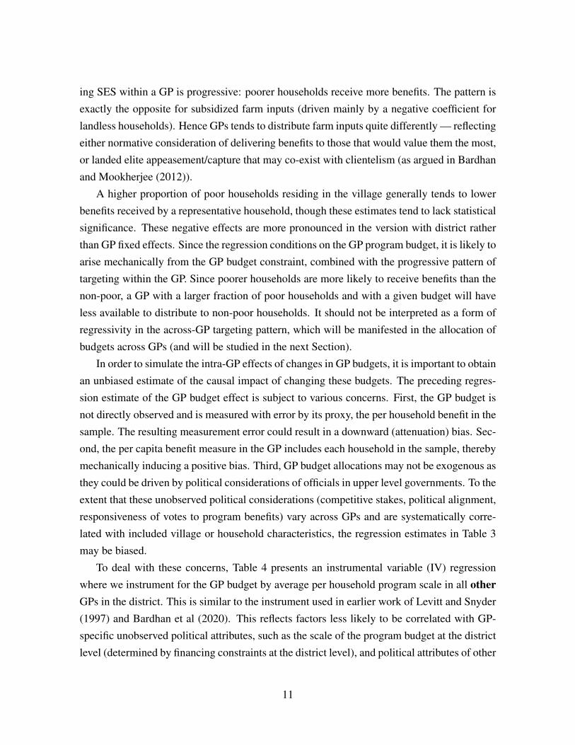
Since the IV estimates indicate negligible bias in the non-IV regression, we use the latter

for our analysis. Table 5 enriches the specification to allow for interactions between GP

budget and household poverty status so as to enhance the predictive accuracy of the model.

These interaction coefficients are negative, implying that while poor households continue

to receive priority, this priority diminishes as the GP budget expands — increases in the

4See Bardhan et al (2020) for details of the first stage regressions and the strength of the instrument inpredicting variation in GP budgets.

12

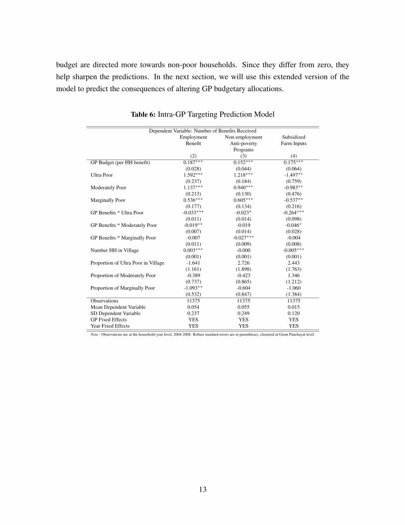
budget are directed more towards non-poor households. Since they differ from zero, they

help sharpen the predictions. In the next section, we will use this extended version of the

model to predict the consequences of altering GP budgetary allocations.

Table 6: Intra-GP Targeting Prediction Model

Dependent Variable: Number of Benefits ReceivedEmployment Non-employment Subsidized

Benefit Anti-poverty Farm InputsPrograms

(2) (3) (4)GP Budget (per HH benefit) 0.187∗∗∗ 0.152∗∗∗ 0.175∗∗∗

(0.028) (0.044) (0.064)Ultra Poor 1.592∗∗∗ 1.218∗∗∗ -1.497∗∗

(0.237) (0.184) (0.759)Moderately Poor 1.137∗∗∗ 0.940∗∗∗ -0.983∗∗

(0.213) (0.130) (0.476)Marginally Poor 0.536∗∗∗ 0.605∗∗∗ -0.537∗∗

(0.177) (0.134) (0.216)GP Benefits * Ultra Poor -0.033∗∗∗ -0.023∗ -0.264∗∗∗

(0.011) (0.014) (0.098)GP Benefits * Moderately Poor -0.019∗∗ -0.019 -0.046∗

(0.007) (0.014) (0.028)GP Benefits * Marginally Poor -0.007 -0.027∗∗∗ -0.004

(0.011) (0.009) (0.008)Number HH in Village 0.003∗∗∗ -0.000 -0.005∗∗∗

(0.001) (0.001) (0.001)Proportion of Ultra Poor in Village -1.641 2.726 2.443

(1.161) (1.898) (1.763)Proportion of Moderately Poor -0.389 -0.423 1.346

(0.737) (0.865) (1.212)Proportion of Marginally Poor -1.093∗∗ -0.604 -1.060

(0.532) (0.847) (1.384)Observations 11375 11375 11375Mean Dependent Variable 0.054 0.055 0.015SD Dependent Variable 0.237 0.249 0.120GP Fixed Effects YES YES YESYear Fixed Effects YES YES YES

Note.- Observations are at the household-year level, 2004-2008. Robust standard errors are in parentheses, clustered at Gram Panchayat level.

13

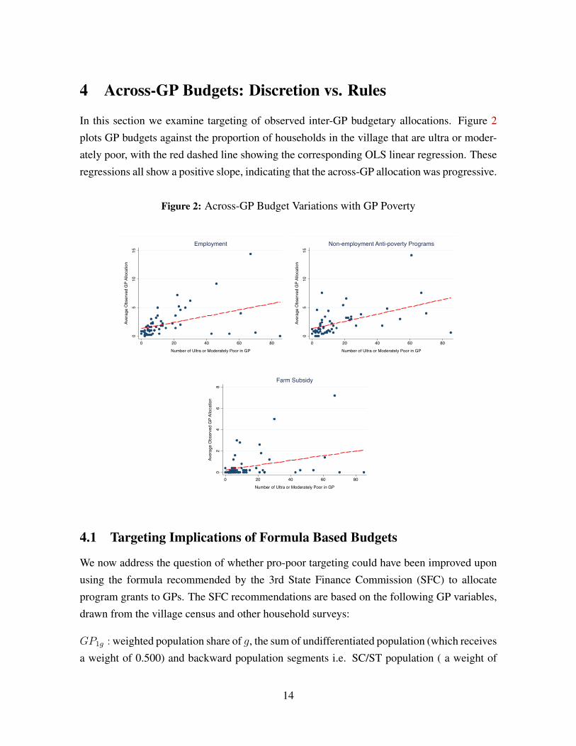
4 Across-GP Budgets: Discretion vs. Rules

In this section we examine targeting of observed inter-GP budgetary allocations. Figure 2

plots GP budgets against the proportion of households in the village that are ultra or moder-

ately poor, with the red dashed line showing the corresponding OLS linear regression. These

regressions all show a positive slope, indicating that the across-GP allocation was progressive.

Figure 2: Across-GP Budget Variations with GP Poverty

05

1015

Aver

age

Obs

erve

d G

P Al

loca

tion

0 20 40 60 80

Number of Ultra or Moderately Poor in GP

Employment

05

1015

Aver

age

Obs

erve

d G

P Al

loca

tion

0 20 40 60 80


Non-employment Anti-poverty Programs

02

46

8

Aver

age

Obs

erve

d G

P Al

loca

tion

0 20 40 60 80


Farm Subsidy

4.1 Targeting Implications of Formula Based Budgets

We now address the question of whether pro-poor targeting could have been improved upon

using the formula recommended by the 3rd State Finance Commission (SFC) to allocate

program grants to GPs. The SFC recommendations are based on the following GP variables,

drawn from the village census and other household surveys:

GP1g : weighted population share of g, the sum of undifferentiated population (which receives

a weight of 0.500) and backward population segments i.e. SC/ST population ( a weight of

14

0.098);

GP2g : female non-literates share of g;

GP3g : food insecurity share of g, calculated from 12 proxy indicators collected in a 2005

Rural Household Survey, based on survey responses to questions such as “do you get less

than one square meal per day for major part of the year?" ;

GP4g : population share of marginal workers, those employed less than 183 days of work in

any of the four categories: cultivators, agricultural labour, household based economic activi-

ties and others;

GP5g : total population without drinking water or paved approach or power supply share of

g;

GP6g : sparseness of population (inverse of population density) share of g.

Table 7 shows how well these characteristics predict the proportion of households in dif-

ferent poverty groups in any given GP. The ultra-poor ratio is rising in the SC/ST proportion

and population sparseness, but not significantly varying with the other SFC characteristics;

the overall R-squared of this regression is 45%. So most of the variation in ultra-poor inci-

dence is not explained. A larger fraction of variation (about two-thirds) in the moderately poor

proportion is explained; most of this predictive power comes from a sharp positive slope with

respect to village population size. The size of the other two groups is predicted less precisely

(R-squared below 40%) by the SFC characteristics, with none of the individual characteristics

being individually significant. These facts highlight the paucity of information available to

construct formulae for programmatic GP budgets.

The specific formula recommended by the SFC for bg resources to be allocated to GP g

is:

bg = 0.598 ∗ GP1g +4∑

i=20.100 ∗ GPig +

6∑j=5

0.051 ∗ GPjg (1)

We apply this formula to calculate recommended budgets, upon assigning weights to GPs

based on their scores using (1) and reallocating district program scales across these GPs in the

same ratio as their respective weights. The deviation of the observed from the recommended

GP budgets are plotted in Figure 3 against the proportion of (ultra or moderately) poor house-

holds within the GP. We fit a quadratic regression whose predicted values are depicted by the

red dashed line. Over the relevant range with less than 40% poor, we see that the regression

15

Table 7: Demographic Share of Poverty Groups and SCF GP Characterisitcs

Ultra Moderately Marginallly Non-poorPoor Poor Poor (4)(1) (2) (3) (4)

Population 0.013 0.472∗∗ 0.042 0.172(0.111) (0.178) (0.790) (0.836)

SC/ 0.141∗∗ 0.021 -1.896 -2.086(0.063) (0.143) (1.450) (1.489)

Female Illiteracy -0.106 0.335 1.453 1.455(0.212) (0.276) (1.216) (1.051)

Food Insecurity -0.030 -0.054 -0.491 -0.109(0.042) (0.090) (0.315) (0.331)

Lack of Infrastructure -0.032 -0.230 0.881 0.469(0.239) (0.344) (1.533) (1.406)

Marginal Workers -0.029 -0.040 1.100 0.889(0.085) (0.147) (0.805) (0.844)

Sparseness of Population 0.435∗∗ 0.266 0.409 0.707(0.180) (0.229) (0.706) (0.885)

Observations 56 56 56 56Adjusted R2 0.449 0.649 0.387 0.333

is upward sloping, starting with a negative intercept and and becoming positive after 10%.

Hence the SFC recommended budgets were less progressive than the observed allocations.

Evidently, political discretion of ULGs ended up creating a more pro-poor targeting pattern

than was recommended by the SFC.

Next, using the intra-GP targeting pattern estimates shown in Table 5, we predict the num-

ber of benefits each household would receive, had the observed GP budget been replaced by

the SFC recommended budget. We then aggregate the observed and predicted benefits from

formula based grants across the entire sample, and compare the two for the average household

in a given group. These results along with corresponding 95% confidence interval bands are

shown in Figure 4. They confirm what one might expect from the greater progressivity of the

observedGP budgets compared with the recommended ones — the use of the SFC formula

would have resulted in less targeting towards the poor. This effect is statistically significant

for non-employment anti-poverty programs, for the ultra-poor and moderately poor groups.

However the effects though negative are not statistically significant for the employment pro-

gram, and are negligible for farm subsidies.

The corresponding implications for a related but slightly different measure of targeting —

the average share of benefits of a given type delivered to poor groups — are shown in Table

8. The SFC formula would have raised the aggregate share of employment benefits for ultra

poor households by 0.53 percentage points, and lowered it by 0.92 percentage points for the

moderately poor group. Aggregating the share of these two groups, there would have been

no improvement at all. The same is true for the the non-employment anti-poverty programs,

16

while it would have raise the combined share slightly for the farm subsidy program.

Figure 3: Deviation of Observed from SFC Recommended GP Budgets

-2-1

01

2

Obs

erve

d - R

ecom

men

ded

GP

Allo

catio

n

0 20 40 60 80


Employment

-4-2

02

4

Obs

erve

d - R

ecom

men

ded

GP

Allo

catio

n

0 20 40 60 80



-1.5

-1-.5

0.5

1

Obs

erve

d - R

ecom

men

ded

GP

Allo

catio

n

0 20 40 60 80


Farm Subsidy

Table 8: Aggregate Shares under Observed and Recommended Allocations

Demographic Employment Non-emp Anti-Pov. Farm SubsidyGroup Share Observed Rec. Observed Rec. Observed Rec.Ultra Poor 8.53 16.57 17.10 14.95 14.03 1.28 1.39Moderately Poor 27.56 35.31 34.78 33.24 33.10 11.63 12.06Marginally Poor 38.33 32.28 32.25 32.81 33.34 39.19 38.66Non-poor 25.58 15.84 15.87 19.00 19.54 47.90 47.88

17

Figure 4: Comparing Observed and Recommended Predicted Allocations

.02

.04

.06

.08

.1Av

g. P

redi

cted

Num

ber o

f Em

ploy

men

t Ben

efits

nonpoor slightly moderate ultra

Observed Recommended

Employment Benefits

.04

.06

.08

.1.1

2Av

g. P

redi

cted

Num

ber o

f Ant

i-pov

erty

Ben

efits




-.15

-.1-.0

50

.05

.1Av

g. P

redi

cted

Num

ber o

f Min

ikits



Farm Subsidies

18

4.2 Alternative Formulae and Aggregate Share of Poor Households

We now examine whether alternative formulae based on changing the weights on GP demo-

graphic variables can improve targeting of benefits to poorer groups compared to observed

allocations. The set of GP characteristics used are the same as ones in equation 1. We draw

10,000 alternative weights from the Dirichlet distribution using a likelihood model with uni-

form density over each weight in the simplex defined by∑

i wi = 1; wi > 0 in R7.

For each draw, we calculate the aggregate share of benefits going to ultra poor and moder-

ately poor households. Figure 6 plots the aggregate shares of the two groups implied by each

alternative formula. The pair of aggregate shares implied by recommended SFC formula is

depicted in red and the pair of shares implied by observed household allocation is depicted by

dashed black lines. The horizontal and vertical lines depicting observed allocation partition

the graph into four. The upper right quadrant depicts the set of weights where the aggregate

share of benefits for both the ultra and moderately poor is higher than the observed allocation.

For employment benefits, none of the drawn weights simultaneously increase the ag-

gregate share of ultra poor and moderately poor households. The southeast quadrant, which

contains the recommended allocation, consists of all weights that improve the aggregate share

of ultra poor compared to observed allocation at the cost of reducing the aggregate share of

moderately poor households.

The upper right panel in Figure 6 plots the aggregate share of non-employment anti-

poverty benefits for ultra and moderately poor households implied by randomly drawn weights.

As noted previously, the aggregate shares implied by the observed allocation are higher than

the shares implied by the SFC-recommended formula. However, the dots in the northeast

quadrant (comprising 18% of the randomly drawn weights) represent alternative weights

which improve the share of both groups simultaneously. Table 9 characterizes these 1829

randomly drawn weights. On average, the alternative weights assign a substantially higher

weight on the SC/ST population share of GP and a lower weight on population size, com-

pared to the recommended weights. The weight that maximizes the aggregate share of ultra

poor allocates 16.05 percent to ultra poor and 34.36 to moderately poor. Incidentally, this

weight also maximizes the aggregate share of the moderately poor. Choosing this vector of

weights would increase the aggregate share of both groups by 1.1 percentage points.

The lower panel in Figure 6 plots the aggregate share of farm subsidies for ultra and mod-

erately poor households implied by randomly drawn weights. The aggregate shares implied

19

Figure 5: Alternative Formula Weights and Aggregate Share of Poor Households.3

.32

.34

.36

Aggr

egat

e Sh

are

of o

f Mod

erat

ely

Poor

.1 .12 .14 .16 .18

Aggregate Share of Ultra Poor

Recommended Allocation Observed Allocation

Employment Benefits

.325

.33

.335

.34

.345

Aggr

egat

e Sh

are

of o

f Mod

erat

ely

Poor

.13 .14 .15 .16



Non-employment Anti-poverty Benefits

.06

.08

.1.1

2.1

4

Aggr

egat

e Sh

are

of o

f Mod

erat

ely

Poor

.005 .01 .015 .02



Farm Subsidies

Table 9: Non-employment Anti-poverty Benefits, Summary Statistics of Alternative Weights

Rec. Summary Statistics: Alternative WeightsFormula count mean sd median max min

Aggregate SharesModerately Poor 0.331 1829 0.335 0.002 0.334 0.344 0.332Ultra Poor 0.140 1829 0.152 0.002 0.152 0.160 0.150Weightsw1: Population 0.500 1829 0.069 0.058 0.054 0.315 0.000w2: SC/ST 0.098 1829 0.315 0.123 0.305 0.812 0.049w3: Female Illiteracy 0.100 1829 0.148 0.127 0.114 0.707 0.000w4: Food insecurity 0.100 1829 0.111 0.097 0.083 0.561 0.000w5: Marginal workers 0.100 1829 0.135 0.116 0.105 0.667 0.000w6: Lack of infrastructure 0.051 1829 0.148 0.123 0.116 0.709 0.000w7: Sparseness of pop. 0.051 1829 0.073 0.059 0.060 0.335 0.000

20

Table 10: Farm Subsidies: Summary Statistics of Alternative Weights

Rec. Summary Statistics: Alternative WeightsFormula count mean sd median max min

Aggregate SharesModerately Poor 0.121 3691 0.128 0.005 0.127 0.143 0.121Ultra Poor 0.014 3691 0.016 0.001 0.016 0.021 0.014Weightsw1: Population 0.500 3691 0.164 0.129 0.133 0.680 0.000w2: SC/ST 0.098 3691 0.077 0.064 0.061 0.363 0.000w3: Female Illit 0.100 3691 0.144 0.125 0.108 0.752 0.000w4: Food insecurity 0.100 3691 0.115 0.099 0.089 0.649 0.000w5: Marginal workers 0.100 3691 0.107 0.090 0.084 0.520 0.000w6: Lack of infrastructure 0.051 3691 0.140 0.121 0.106 0.669 0.000w7: Sparseness of population 0.051 3691 0.253 0.123 0.238 0.751 0.029

by the observed allocation perform worse than the shares implied by recommended formula.

About 37% of the randomly drawn weights improve aggregate shares for the two poor groups

compared to observed allocation. These are depicted by the set of weights in the upper right

quadrant of the graph. Table 10 characterizes these 3691 randomly drawn weights. On an

average, the alternative weights put a substantially higher weight on sparseness of population

share of GPs and a substantially less weight on population of the GP compared to the rec-

ommended weights. The weight that maximizes the shares of the two groups increases the

share of ultra poor only by 0.8 percentage points and the share of moderately poor by 2.7

percentage points.

Finally, Figure 6 plots the predicted number of benefits for each poverty group if the

formula weights had been chosen to maximize the average share of the ultra-poor group. For

the employment and farm program there is hardly any change. For the non-employment non-

farm programs, the expected benefits of the two poorest groups would have been higher, and

these effects are statistically significant. For an ultra-poor household, the expected number of

benefits would have increased from .10 to .13.

21

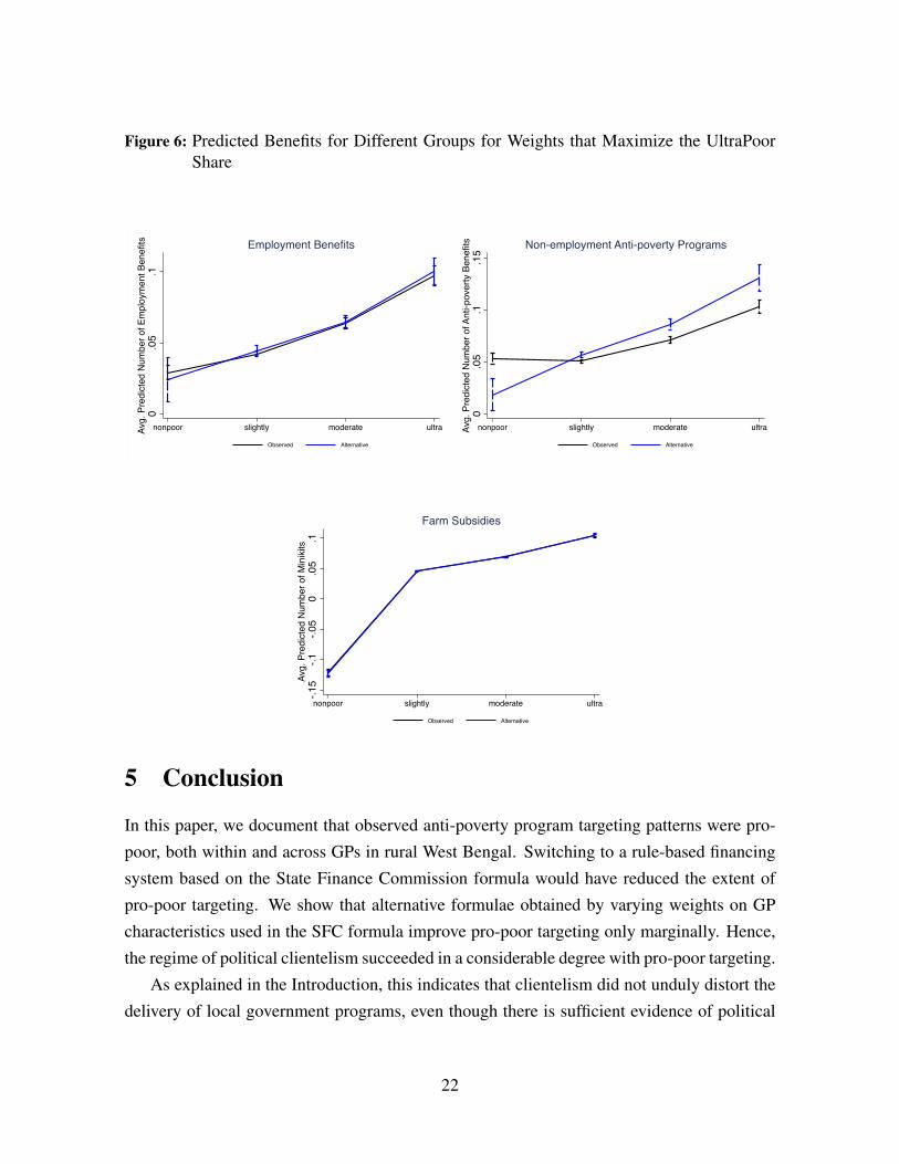
Figure 6: Predicted Benefits for Different Groups for Weights that Maximize the UltraPoorShare

0.0

5.1

Avg.

Pre

dict

ed N

umbe

r of E

mpl

oym

ent B

enefi

ts


Observed Alternative

Employment Benefits

0.0

5.1

.15

Avg.

Pre

dict

ed N

umbe

r of A

nti-p

over

ty B

enefi

ts




-.15

-.1-.0

50

.05

.1Av

g. P

redi

cted

Num

ber o

f Min

ikits



Farm Subsidies

5 Conclusion

In this paper, we document that observed anti-poverty program targeting patterns were pro-

poor, both within and across GPs in rural West Bengal. Switching to a rule-based financing

system based on the State Finance Commission formula would have reduced the extent of

pro-poor targeting. We show that alternative formulae obtained by varying weights on GP

characteristics used in the SFC formula improve pro-poor targeting only marginally. Hence,

the regime of political clientelism succeeded in a considerable degree with pro-poor targeting.

As explained in the Introduction, this indicates that clientelism did not unduly distort the

delivery of local government programs, even though there is sufficient evidence of political

22

discretion used by upper level governments who manipulated GP budgets in line with their

re-election motives. It was not the case, for instance, that re-election concerns ended up fa-

voring less poor regions or households owing to their greater inclination to respond to benefits

received by switching their votes to the local incumbent. Hence, using pro-poor targeting as a

welfare criterion, the political distortions entailed by clientelism imposed a low welfare cost.

A number of qualifications are in order. The public interest includes many other con-

siderations apart from pro-poor targeting or more broadly vertical equity in the distribution

of private benefits. Politically manipulated variations in GP budgets result in horizontal in-

equity — unequal treatment of different GP areas in ways that cannot be defended on norma-

tive grounds, and reduce the legitimacy of incumbent parties. In addition, focusing alone on

pro-poor targeting alone would ignore possible under-provision of public goods and reduced

political competition that has been alleged by many scholars to be pernicious consequences

of clientelism. However, additional research is needed to assess the empirical relevance of

these concerns.

References

Azulai, M. (2017), “Public good allocation and the welfare cost of political connections: ev-

idence from Brazilian matching grants," Working Paper, Institute of Fiscal Studies, London.

Bardhan P, D. Mookherjee and M. Parra Torrado (2010), “Impact of Political Reservations

in West Bengal Local Governments on Anti-Poverty Targeting," Journal of Globalization and

Development.

Bardhan P and D. Mookherjee (2012), “Political Clientelism and Capture: Theory and Evi-

dence from West Bengal," working paper, Institute for Economic Development, Boston Uni-

versity.

Bardhan P, D. Mookherjee, M. Luca and F. Pino (2014), “Evolution of Land Distribution

in West Bengal 1967–2003: Role of Land Reform and Demographic Changes”, Journal of

Development Economics, 2014.

Bardhan P., S. Mitra, D. Mookherjee and A. Sarkar (2015), “Political Participation, Clien-

telism, and Targeting of Local Government Programs: Results from a Rural Household Sur-

vey in West Bengal, India," in Is Decentralization Good For Development? Perspectives from

Academics and Policy Makers, Edited by Jean-Paul Faguet and Caroline Poschl, Oxford: Ox-

ford University Press,

23

Bardhan P, S. Mitra, D. Mookherjee and A. Nath (2020), “ How Do Voters Respond to Wel-

fare Programs vis-a-vis Infrastructure Programs? Evidence for Clientelism in West Bengal,"

working paper, Institute for Economic Development, Boston University.

Dey S. and K. Sen (2016), "Is Partisan Alignment Electorally Rewarding? Evidence from

Village Council Elections in India," IZA Discussion Paper No. 9994.

Dreze J., R. Khera and A. Somanchi (2020), “Balancing Corruption and Exclusion: A Rejoin-

der," Ideas for India, https://www.ideasforindia.in/topics/poverty-inequality/balancing-corruption-

and-exclusion-a-rejoinder.html.

Finan, F. and Mazzocco, M. (2020), ‘Electoral incentives and the allocation of public funds,"

Working Paper, Department of Economics, University of California, Berkeley.

Levitt S. and J. Snyder (1997), “The Impact of Federal Spending on House Election Out-

comes," Journal of Political Economy, 105(1), 30-53.

Shenoy A. and L. Zimmerman (2020), “Political Organizations and Persistent Policy Distor-

tions," working paper, Department of Economics, University of California, Santa Cruz.

Tarquinio L. (2020), “The Politics of Drought Relief: Evidence from South India," working

paper, Department of Economics, Boston University.

24

clientelistic politics and pro-poor targeting: rules

Documents