click here full article a semidiscrete finite volume

2 A semidiscrete finite volume formulation for multiprocess

3 watershed simulation

4 Yizhong Qu1 and Christopher J. Duffy1

5 Received 26 November 2006; revised 30 April 2007; accepted 9 May 2007; published XX Month 2007.

6 [1] Hydrological processes within the terrestrial water cycle operate over a wide range of7 time and space scales, and with governing equations that may be a mixture of ordinary8 differential equations (ODEs) and partial differential equations (PDEs). In this paper we9 propose a unified strategy for the formulation and solution of fully coupled process10 equations at the watershed and river basin scale. The strategy shows how a system of11 mixed equations can be locally reduced to ordinary differential equations using the12 semidiscrete finite volume method (FVM). Domain decomposition partitions the13 watershed surface onto an unstructured grid, and vertical projection of each element forms14 a finite volume on which all physical process equations are formed. The projected15 volume or prism is partitioned into surface and subsurface layers, leading to a fully16 coupled, local ODE system, referred to as the model ‘‘kernel.’’ The global ODE system is17 assembled by combining the local ODE system over the domain, and is then solved by a18 state-of-the-art ODE solver. The unstructured grid, based on Delaunay triangulation, is19 generated with constraints related to the river network, watershed boundary, elevation20 contours, vegetation, geology, etc. The underlying geometry and parameter fields are then21 projected onto the irregular network. The kernel-based formulation simplifies the process22 of adding or eliminating states, constitutive laws, or closure relations. The strategy is23 demonstrated for the Shale Hills experimental watershed in central Pennsylvania, and24 several phenomena are observed: (1) The enslaving principle is shown to be a useful25 approximation for soil moisture–water table dynamics for shallow soils in upland26 watersheds; (2) the coupling shows how antecedent moisture (i.e., initial conditions) can27 amplify peak flows; (3) the coupled equations predict the onset or threshold for upland28 ephemeral channel flow; and (4) the model shows how microtopographic information29 controls surface saturation and connectivity of overland flow paths for the Shale Hills site.30 The open-source code developed in this research is referred to as the Penn State Integrated31 Hydrologic Model (PIHM).

33 Citation: Qu, Y., and C. J. Duffy (2007), A semidiscrete finite volume formulation for multiprocess watershed simulation, Water

34 Resour. Res., 43, XXXXXX, doi:10.1029/2006WR005752.

36 1. Introduction

37 [2] In this paper we address the problem of process38 integration for hydrologic prediction in watersheds and river39 basins. Simulation is now widely utilized as a complemen-40 tary research methodology to theory and experiment [Post41 and Votta, 2005]. However, the grid resolution, scale of the42 model, and range of hydrologic processes operating in43 watersheds and river basins offer the dilemma of what is44 necessary to predict hydrologic response or to simulate45 certain behaviors of the coupled system. In this paper we46 formulate a multiscale strategy that incorporates constitutive47 relationships representing volume-average state variables.48 For small watersheds and fine numerical grids, local contin-49 uum relationships (e.g., Darcy’s law) lead to a fully coupled,

50physics-based, distributed model. At larger scales and coarse51grids, empirical relationships with large-scale volume aver-52ages are applied, and the model becomes a semidistributed53model. A brief review of hydrologic modeling strategies54demonstrates the issues involved with integration and cou-55pling of multiple processes and clarifies the purpose of this56paper.57[3] Current hydrologic models may be described from58two perspectives: physically based, spatially distributed59models, and lumped conceptual models. Freeze and Harlan60[1969] developed the first blueprint for numerical solutions61to physically based, distributed watershed models starting62from a continuum perspective (i.e., Richards’ equations for63subsurface flow, Saint Venant equations for surface flow and64channel routing). It was some years before the SHE model65[Abbott et al., 1986a, 1986b] and its variants produced a66second generation where the coupled physical equations are67actually solved on a regular grid, with coupling handled68through a sophisticated control algorithm that passes infor-69mation between processes (e.g., surface water–groundwater70exchange).

1Department of Civil and Environmental Engineering, PennsylvaniaState University, University Park, Pennsylvania, USA.

Copyright 2007 by the American Geophysical Union.0043-1397/07/2006WR005752$09.00

XXXXXX

WATER RESOURCES RESEARCH, VOL. 43, XXXXXX, doi:10.1029/2006WR005752, 2007ClickHere

for

FullArticle

1 of 18

http://dx.doi.org/10.1029/2006WR005752

71 [4] The approach of coupling multiple processes through72 time-lagging and iterative coupling through boundary73 conditions is generally considered a weak form of coupling,74 in that it may lead to significant instability and errors75 [LaBolle et al., 2003]. The approach also requires consider-76 able reprogramming if changes are made to the physical77 equations for a specific application. More recently, Panday78 and Huyakorn [2004] have developed an approach where all79 equations in the model are of the diffusive type, which are80 solved in a single system on a regular grid (e.g., Richard’s81 equation and diffusive wave equation), while equations for82 other processes (vegetation, energy, snow) are dealt with83 separately (iteratively). Yeh et al. [1998] have used a similar84 approach but with finite elements. As will be described later,85 our approach couples all dynamical equations within the86 same prismatic volume (a prism is defined by a triangle87 projected from the canopy, through the land surface to the88 lower boundary of groundwater flow); and all equations are89 solved simultaneously, eliminating the need for a controller,90 delayed, or off-line process equations.91 [5] Lumped or spatially integrated models are widely92 used today, where the goal of the prediction is outflow93 from forcing (e.g., rainfall-runoff, recharge-baseflow,94 precipitation-infiltration). Lumped systems are low-95 dimensional and conveniently solved, but still require an96 empirical relationship for flux discharge that is generally97 assumed to be linear or weakly nonlinear and fitted or98 calibrated to the data. The reduced parameter set of this99 approach can resolve the overall mass balance but cannot by100 definition inform the internal space-time variation of phys-101 ical processes. The Stanford watershed model is an early102 example of the lumped model that includes watershed103 processes [Crawford and Linsley, 1966]. There have been104 efforts to try to bridge these two approaches. Duffy [1996]105 describes a two-state model by integrating Richards’ equa-106 tion over a hillslope into saturated and unsaturated states,107 and later extended this approach to the problem of moun-108 tain-front recharge using hypsometry to partition the upland,109 transition, and flood plain zones into a intermediate-110 dimensional system [Duffy, 2004]. Reggiani et al. [1998,111 1999] proposed a comprehensive semidistributed frame-112 work in which integrated conservation equations of mass,113 momentum, and energy are solved over a representative114 elementary watershed (REW). They discuss the issues115 involved in parameterizing the integral flux-storage relation116 at the REW scale, and refer to this as hydrologic closure.117 [6] The decision of using a lumped, distributed, or semi-118 distributed approach to model watershed systems ultimately119 depends on the purpose of the model, and each has its120 advantages and disadvantages. For the distributed case, the121 governing equations are derived from local constitutive122 relationships. For instance, the Darcy equation is applicable123 at the plot or perhaps hillslope scale, but it is not clear what124 should be the effective relation of flux-to-state variable125 when integrated over larger scales where semidistributed126 or lumped models are used (e.g., the hydrologic closure127 problem discussed by Beven [2006]). At present there is128 considerable discussion in the literature about the relation of129 data needs and predictive models, including the issues of130 model type (lumped, semidistributed, distributed), unique-131 ness, and the appropriate scales of integration [Sivapalan et132 al., 2002].

133[7] In the present paper a new strategy for integrated134hydrologic modeling is proposed that naturally handles135physical processes of mixed partial differential equations136(PDEs) and ordinary differential equations (ODEs) as a137fully coupled system. The model formulates the local138physical equations via the finite volume method, using139geographic information systems (GIS) tools to decompose140the model domain on an unstructured grid, as well s141distributing a priori parameter estimates to each grid cell.142In the limit of small-scale numerical grids, the finite volume143method implements classical (e.g., contiuum) constitutive144relationships. For larger grid scales the method reflects the145assumptions of the semidistributed approach described146above, but with full coupling of all elements. The process147of altering the physical model to accommodate effective148parameterizations or new equations is a relatively simple149process, since all equations reside in the same location in150the code (i.e., the kernel). In this approach, the interactions151are assembled on the right-hand side of the global ODE152system, which is then solved with a state-of-the-art solver153designed for stiff, nonlinear systems. The approach utilizes154a triangular irregular grid that covers the domain with the155fewest number of triangles [Palacios-Velez and Duevas-156Renaud, 1986; Polis and McKeown, 1993] subject to157constraints as defined by the particular problem.

1582. Modeling Approach

1592.1. Semidiscrete FVM Approach

160[8] In this section we develop the finite volume approx-161imation for an arbitrary physical process operating on an162unstructured grid cell. A general form of the mass conser-163vation equation for an arbitrary scalar state variable c can164be written

@c@t

þr � cVþ @c@z

¼ Wc; ð1Þ

166where c represents mass fraction of storage (dimension-167less). For convenience, the velocity vector in (1) is divided168into horizontal (V = {u, v}) and vertical components {w},169and Wc is a local source/sink term for the process170represented by c. Volume integration of (1) proceeds in171two steps: First, we integrate over the depth of the layer and172then over the area. For a single layer of thickness za � z � zb173containing the scalar c, the integral over the depth takes the174form

@

@t

Zzbza

cdz� czb

@zb@t

þ cza

@za@t

þrZzbza

cVdz� Vcð Þzbrzb

þ Vcð Þzarza þ wcð Þza� wcð Þzb ¼Zzbza

Wcdz ð2Þ

176We can evaluate the boundary terms, by rewriting177equation (2) for a small layer about the boundary itself,178zb

� � zb � zb+, where zb

� = zb � e and zb+ = zb + e. Letting the

179layer thickness approach zero, zb+ � zb

� ! 0, the integral180terms are eliminated and the remaining terms must balance

2 of 18

XXXXXX QU AND DUFFY: MULTIPROCESS WATERSHED SIMULATION XXXXXX

181 as we approach the interface from both sides, leading to a182 definition of the net interface flux:

cbþ@zbþ

@tþ Vcð Þbþrzbþ � wcð Þbþ¼ cb�

@zb�

@t

þ Vcð Þb�rzb� � wcð Þb�¼ Qb; ð3Þ

184 where Qb is the net flux across z = zb. A similar expression185 is found for Qa at z = za. Equation (2) is now written in186 terms of vertically integrated storage in the layer:

@c@t

þr Vcð Þ ¼ Qb � Qa þ w; ð4Þ

188 where c is the volumetric storage per unit area (L) in the189 layer defined by

c ¼Zzbza

cdz; ð5Þ

191 and w is the vertically integrated source/sink term

w ¼Zzbza

Wcdz: ð6Þ

193 To complete the volume integration, equation (4) is now194 written

@

@t

ZA

cdAþZG

N Vcð ÞdG ¼ZA

Qb � Qa þ wð ÞdA; ð7Þ

196 where the divergence theorem was applied to the second197 term, G is the perimeter of A, and N is the unit normal vector198 on G. Writing (7) in semidiscrete finite volume form199 [Leveque, 2002] yields

dcdt

¼X2k¼1

Qk �Xmi¼1

Qi; ð8Þ

201 where c is now interpreted as the volumetric storage (L3) of202 c in the control volume (incompressible fluid), Qi is net203 volumetric flux through the sides i = 1, 2, 3 of the control204 volume, and Qk is the net volumetric flux across the upper205 and lower boundaries k = 1, 2. Later it will be convenient to206 divide (8) by the projected horizontal surface area of the207 finite volume such that storage is an equivalent depth, and208 volumetric flux terms are normalized to a unit horizontal209 surface area.210 [9] The vector form of equation (8) represents all pro-211 cesses c = {c1, c2,. . .ck} within the control volume and212 forms a fully coupled local ODE system. The fluxes across213 the sides of the control volume are evaluated by appropriate214 constitutive (or closure) relationships for specific processes215 and applications. We note again that the finite volume216 method guarantees mass conservation for each control217 volume [Leveque, 2002], and that the semidiscrete repre-218 sentation reduces all equations to a standard form.219

2202.2. Multiscale, Multiprocess Formulation

221[10] The next step in developing the multiprocess system222is domain decomposition. The horizontal projection of the223watershed area is decomposed into Delauney triangles. Each224triangle is projected vertically to span the ‘‘active flow225volume’’ forming a prismatic volume which is further226subdivided into layers to account for the physical process227equations and material layers. When governing equations228are a mix of ODEs (e.g., vegetation interception) and PDEs229(e.g., overland flow, groundwater flow), the PDEs are first230reduced to ODEs by applying the semidiscrete finite volume231method (FVM) approach described above, and then all232ODEs are associated with a layer within the prism. The233prism is where all physical equations (and thus all time-234scales of the problem) reside, and we refer to this local235system as the kernel. Assembling the local ODE system236over the watershed domain, a global system is formed237which is then solved with an efficient ODE solver. This238solution method is also known as the ‘‘method of lines’’239[Madsen, 1975], here applied to a system of differential240equations. For the multiple processes encountered in water-241shed research, the approach has several advantages. First,242the model kernel representing all physical processes oper-243ating within the prismatic control volume can be easily244modified for different applications or processes without245altering the solver or even the domain decomposition. Since246all physical equations are in a single subroutine, adding or247omitting processes, material properties, or forcing makes248modifications to the program quite simple. Second, the249ODE is solved as a ‘‘fully coupled’’ system, with no time250lagging or iterative linking of processes. Third, alternative251constitutive or closure relationships are also easily imple-252mented and tested in this strategy. The constitutive relation-253ship might come from conceptual models, numerical254experiments [Duffy, 1996], or theoretical derivation255[Reggiani et al., 1999; Reggiani and Rientjes, 2005]. It is256noted that constitutive relationships are sensitive to the scale257of volume integration [Beven, 2006], a feature that is natural258to the semidiscrete approach used here.259[11] In this research we are developing an open-source260community code for the simulation of watersheds and river261basins, and we refer to this code as PIHM: Penn State262Integrated Hydrologic Model. In this first generation of263PIHM, we consider the following processes and dimen-264sions: one-dimensional (1-D) channel routing, 2-D overland265flow, and 2-D subsurface flow are governed by PDEs, while266canopy interception, evapotranspiration, and snowmelt are267described by ODEs. Each process is assigned to a layer268within the kernel with overland flow and channel flow269assigned to the surface layer, and the channel centered on270any edge of the element. Prior to domain decomposition, the271river network, hydraulic structures, or other devices, such as272dams, gages, weirs, etc., are identified as special points used273to constrain the decomposition. Although it imposes some274computational burden to the grid generation, this idea275simplifies the geometry of the decomposed region, which276in turn facilitates assembling the global ODE system. For277example, this step will guarantee that no channel intersects278the control volume interior, or the channel segments are279always centered on the boundary between two watershed280elements. It also locates gages (stage, well level, climate281station) at vertices of elements where desired, simplifying

XXXXXX QU AND DUFFY: MULTIPROCESS WATERSHED SIMULATION

3 of 18

XXXXXX

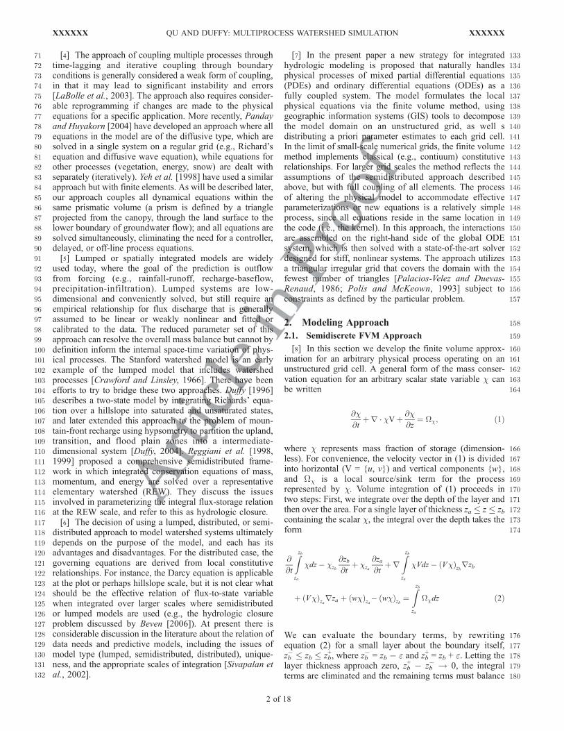
282 postprocessing. Figure 1 illustrates the decomposition and283 kernel for the system to be studied here.

285 3. Building the Local ODE System

286 [12] The choice of equations in any situation is a practical287 balance of the most important physical processes assumed288 to operate on a watershed (Shale Hills, in our case), the289 assumptions made about these processes in a particular290 representation, and the scale of computation. We note that291 there are no intrinsic limitations to more complex (or292 simpler) equations/processes. Those presented here are293 sufficient to characterize the physics of the particular294 physical setting we have chosen to demonstrate.

2963.1. Processes Governed by PDEs

2973.1.1. Surface Overland Flow298[13] The governing equations for surface flow are the 2-D299St. Venant equations. Sleigh et al. [1998] have developed a300numerical algorithm solving the full St. Venant equations301using the finite volume method for predicting flow in rivers302and estuaries, where the normal flux vector is calculated303using Riemann approach [Leveque, 2002], and we follow304their approach here. Letting c ! ho(x, y, t), the vertically305integrated form of the continuity equation (4) is given by

@ho@t

þ @ uhoð Þ@x

þ @ vhoð Þ@y

¼X2k¼1

qk ; ð9Þ

Figure 1. Schematic view of domain decomposition for hillslopes and stream reach. The finite controlvolumes, elements, are prisms projected from the triangular irregular grid also referred to as a TIN(triangular irregular network). The TIN is generated with channels as constraints, which will guaranteethat the channel is along the element boundary. In the upper part of the figure, the basic element is shownto the left with multiple hydrological processes. A channel segment for a triangle bounded by a stream isshown to the right.

4 of 18


331 where ho (x, y, t) is the local water depth. Here u and v are332 velocities in the plane x, y; qk are the surface flux terms333 normalized by surface area. Note that there are three334 unknowns, ho, u, and v, for each element. To reduce the335 complexity of solving the full St. Venant equations, we336 neglect inertia terms in the momentum equation, and337 Manning’s formula is used to close equation (9), which338 yields the diffusion wave approximation [Gottardi and339 Venutelli, 1993]

@ho@t

¼ @

@xhoks

@H

@x

� �þ @

@xhoks

@H

@x

� �þXk

qk ð10Þ

341 with

ks ¼h23o

ns

1

j@H=@sj12

; ð11Þ

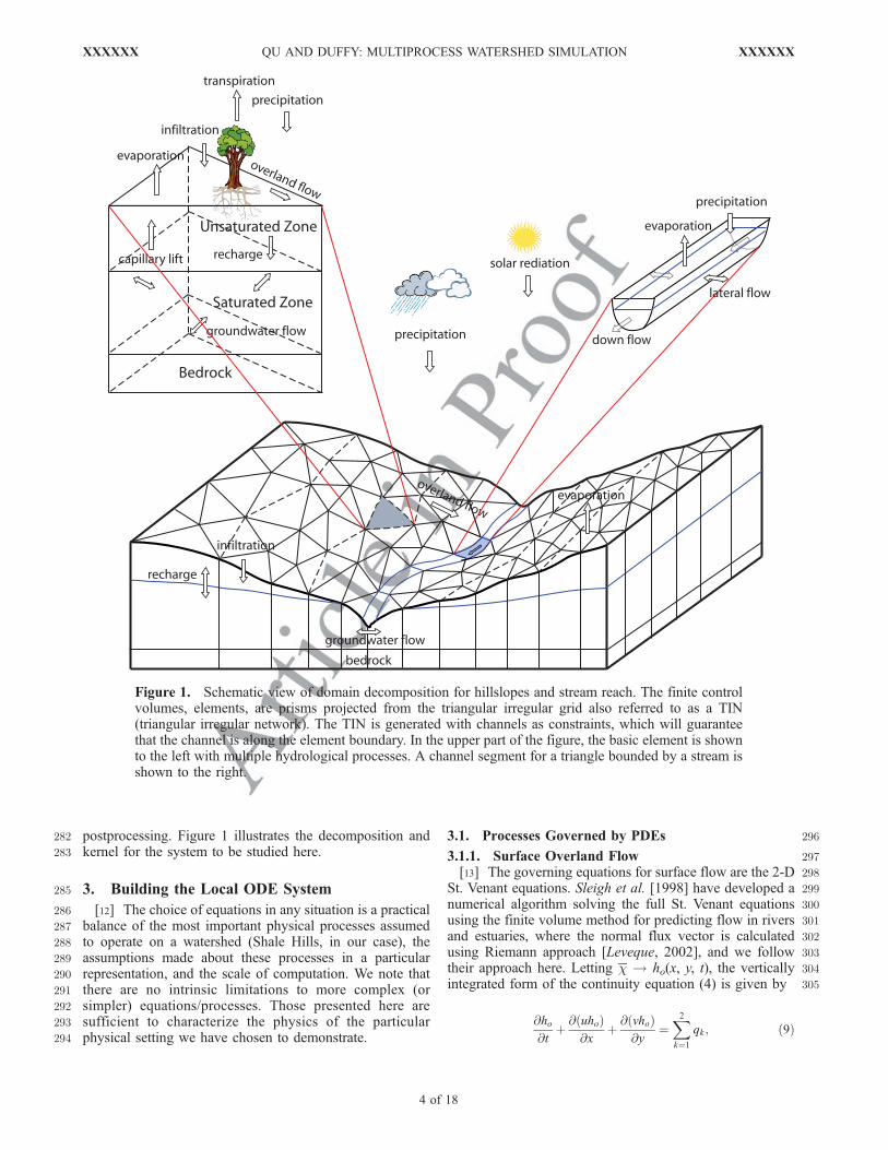
343 where H(x, y, t) is the water surface elevation above an344 horizontal datum, n is Manning roughness coefficients, s =345 s(x, y) is the vector direction of maximum slope, and qk are346 the layer top and bottom input/output.347 [14] Since the basic element in our implementation is a348 vertically projected prism (Figure 1), the evaluation for ks is349 slightly complicated. Let (xi, yi, Hi) be the local coordinates350 of the free water surface at vertex Vi. Assume the free351 surface plane is determined by vertex V2, V3, V4 and that the

352triangular element of D4D7D8 is identical. The plane is then353defined by (see Figure 2)

x y H 1

x2 y2 H2 1

x3 y3 H3 1

x4 y4 H4 1

��

��¼ 0: ð12Þ

355Note that

@H

@s¼ s

k s k � rH ;

357and thus the hydraulic head gradient along the maximum358slope direction of element D4D7D8 is given by

@H

@s¼

ffiffiffiffiffiffiffiffiffiffiffiffiffiffiffiffiffiffiffiffiffiffiffiffiffiffiffiffiffiffiffiffiffiffiffiffiffiffiffiffiffiffiffiffiffiffiffiffiffiffiffiffiffiffiffiffiffiffiffiffiffiffiffiffiffiffiffiffiffiffiffiffiffiffiffiffiffiffiffiffiffiffiffiffiffiffiffiffiffiffiffiffiffiffiffiffiffiffiy3 � y2ð Þ H4 � H2ð Þx2 � x3ð Þ H4 � H2ð Þ

� �2

þ x4 � x2ð Þ H3 � H2ð Þx3 � x2ð Þ H4 � H2ð Þ

� �2s

:

ð13Þ

360For elements that border a channel, special handling is361required, and we discuss this in section 3.1.3. For the362diffusion wave approximation, the surface flux per unit

width of flow is given by

Qs ¼ hoks@H

@s; s ¼ s x; yð Þ ð14Þ

365using (11) and (13). Applying the semidiscrete approach366discussed above to equation (10) and normalizing by the367surface area of the element yields the semidiscrete368approximation for overland flow

dho

dt¼ p� qþ � eþ

X3j¼1

qsj

!i

; ð15Þ

369where qjs is the normalized lateral flow rate from element i

371to its neighbor j. The terms p, q+, and e are throughfall372precipitation, infiltration, and evaporation, respectively.3733.1.2. Subsurface Flow374[15] For subsurface flow we start again from (1) and let375our scalar be the moisture content (volume water/void376volume), c ! q, which we write (1) as

@q@t

þrqV þ @ wqð Þ@z

¼ þSq; ð16Þ

378where once again the divergence terms are separated into379vertical (w) and horizontal or V = (u, v) components. Flow380within the subsurface layer is complicated by the existence381of a free surface boundary or water table within the layer.382The layer is partitioned into two parts, where the soil above383the water table (z+) is governed by gravitational and surface

Figure 2. Delaunay triangulation and Voronoi diagram.The solid lines form Delanunay triangles, and the dashedlines form Voronoi polygons. The circumcenter Vi is thevertex of the perpendicular bisectors of the triangle, and isused to represent the triangle for the volume average of thestate variable.


5 of 18

XXXXXX

384 tension forces, while gravity alone governs below the water385 table (z�). Using (2) and (3) and integrating over the depth386 of the layer yields

qs@hu@t

þr qVhuð Þ ¼ qþ � qo

qs@hg@t

þr qVhg �

¼ qo � q�:

ð17Þ

388 The divergence terms in (17) represent horizontal flow in389 the unsaturated (plus sign) and saturated (minus sign) parts390 of the layer, qs is the moisture content at saturation, hu is the391 equivalent depth of moisture storage above the water table,392 and hg is the depth of saturation below the water table393 defined by

hu ¼Zzbzþo

qqsdz; hg ¼

Zz�oza

qsqsdz; ð18Þ

394 where the layer is now defined with two complementary396 zones above (za � z � zo

+) and below the water table (za �397 z � zo

�). The flux terms or source terms to the soil398 moisture zone (q+ and qo) are defined respectively as399 infiltration/exfiltration through the soil surface, and recharge400 to and from the water table. The flux q� admits an exchange401 with a deeper groundwater layer. The divergence terms for402 lateral flow are evaluated by integrating (17) over the403 projected surface area of the control volume (Figure 1).404 Applying the Reynolds transport theorem [Slattery, 1978]405 and the divergence theorem yields equations for flow above406 and below the water table, respectively:

1

A

Z ZA

r qVhuð ÞdA ¼ 1

A

ZB

qVhuð ÞndB ’X3j¼1

quj

1

A

Z ZA

r qVhg �

dA ¼ 1

A

ZB

qVhg �

ndB ’X3j¼1

qgj :

ð19Þ

408 See Duffy [1996] for details. Finally, the balance equations409 are formed for a fully coupled unsaturated-saturated flow410 within the layer,

qsdhu

dt¼ qþ � qo þ

X3j¼1

quj

qsdhg

dt¼ qo � q� þ

X3j¼1

qgj ;

ð20Þ

412 where the unsaturated and saturated depth of storage (hu, hg)413 are now interpreted as volume averages per unit projected414 horizontal surface area. The divergence terms in (20) define415 the net lateral soil moisture flux and net lateral groundwater416 exchange with adjacent elements. From this point we will417 assume that the flow is vertical in the unsaturated zone, but418 that lateral saturated groundwater flow is

X3j¼1

qgj 6¼ 0:

420 We note that this term also represents stream-aquifer421 interaction for elements adjacent to a channel. The net flux

422to/from the water table q0(hu, hg) represents the integral423properties of unsaturated flow and recharge to/from the424water table, as well as the effect of water table fluctuations.425Again, in the governing ODEs all fluxes are normalized by426projected horizontal surface area of the element with units427[L/T].428[16] For applications where the Darcy relationship is429appropriate, lateral groundwater fluxes are evaluated using430its volume-average form [Duffy, 2004] given by

qgij ¼ BijKeff

Hg

�i� Hg

�j

Dij

hg �

iþ hg �

j

2; ð21Þ

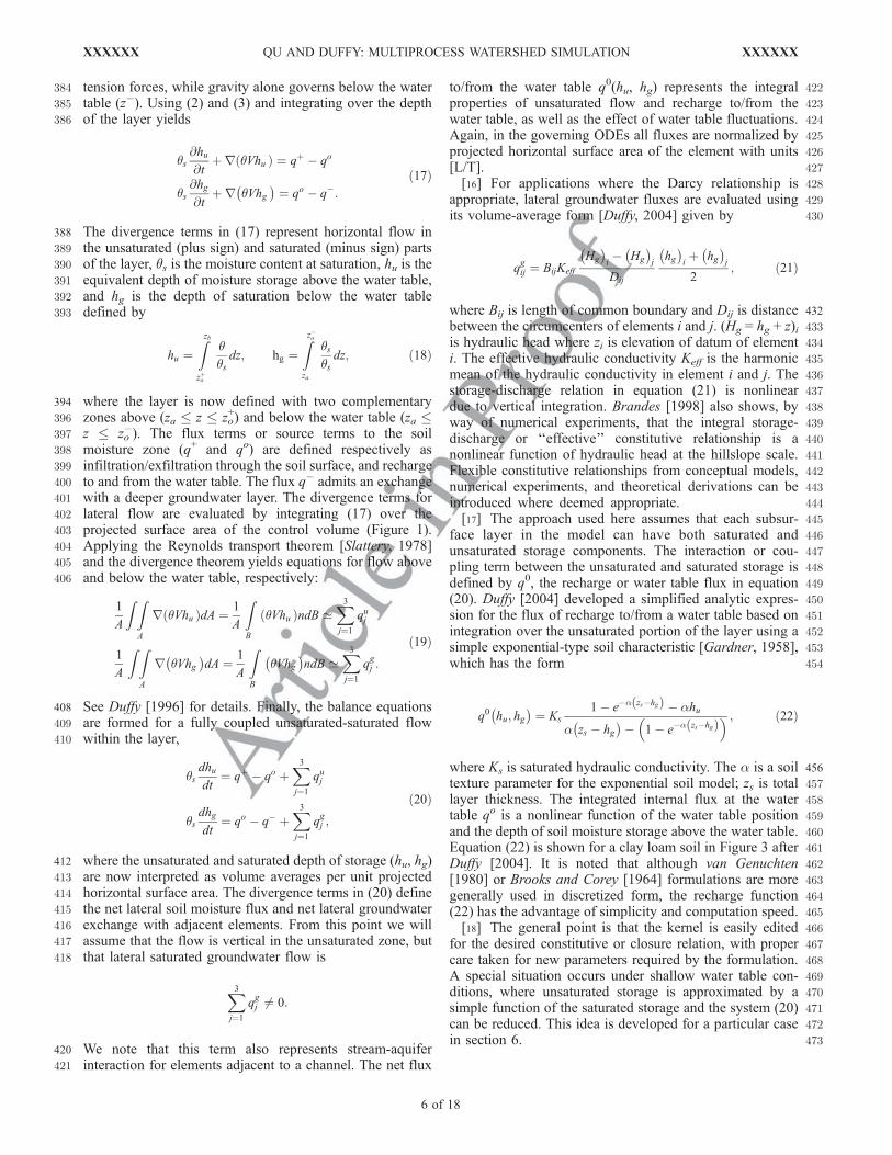
432where Bij is length of common boundary and Dij is distance433between the circumcenters of elements i and j. (Hg = hg + z)i434is hydraulic head where zi is elevation of datum of element435i. The effective hydraulic conductivity Keff is the harmonic436mean of the hydraulic conductivity in element i and j. The437storage-discharge relation in equation (21) is nonlinear438due to vertical integration. Brandes [1998] also shows, by439way of numerical experiments, that the integral storage-440discharge or ‘‘effective’’ constitutive relationship is a441nonlinear function of hydraulic head at the hillslope scale.442Flexible constitutive relationships from conceptual models,443numerical experiments, and theoretical derivations can be444introduced where deemed appropriate.445[17] The approach used here assumes that each subsur-446face layer in the model can have both saturated and447unsaturated storage components. The interaction or cou-448pling term between the unsaturated and saturated storage is449defined by q0, the recharge or water table flux in equation450(20). Duffy [2004] developed a simplified analytic expres-451sion for the flux of recharge to/from a water table based on452integration over the unsaturated portion of the layer using a453simple exponential-type soil characteristic [Gardner, 1958],454which has the form

q0 hu; hg �

¼ Ks

1� e�a zs�hgð Þ � ahu

a zs � hg �

� 1� e�a zs�hgð Þ� ; ð22Þ

456where Ks is saturated hydraulic conductivity. The a is a soil457texture parameter for the exponential soil model; zs is total458layer thickness. The integrated internal flux at the water459table qo is a nonlinear function of the water table position460and the depth of soil moisture storage above the water table.461Equation (22) is shown for a clay loam soil in Figure 3 after462Duffy [2004]. It is noted that although van Genuchten463[1980] or Brooks and Corey [1964] formulations are more464generally used in discretized form, the recharge function465(22) has the advantage of simplicity and computation speed.466[18] The general point is that the kernel is easily edited467for the desired constitutive or closure relation, with proper468care taken for new parameters required by the formulation.469A special situation occurs under shallow water table con-470ditions, where unsaturated storage is approximated by a471simple function of the saturated storage and the system (20)472can be reduced. This idea is developed for a particular case473in section 6.

6 of 18


474 3.1.3. Channel Routing475 [19] For channel routing, applying the semidiscrete ap-476 proach to the 1-D Saint Venant equations with the same477 assumptions as overland flow yields

dhc

dt¼ p� eþ

X2l¼1

qsl þ qgl

�þ qcin � qcout

!i

; ð23Þ

479 where hc is depth of water in the channel, p and e are480 precipitation and evaporation for the channel segment, and481 ql

gand ql

s are the lateral interaction terms for the aquifer and482 surface flow from each side of the channel. The upstream483 and downstream channel segments are qin

c and qoutc ,

484 respectively. The volumetric fluxes are normalized by the485 horizontally projected surface area of the channel segment,486 where the channel is a 1-D prismatic volume with a487 trapezoidal or other cross section. As in the case of overland488 flow, the diffusion wave approximation is applied to the489 upstream and downstream channel flux terms.490 [20] The interaction of surface overland flow and channel491 routing, ql

s in equation (15) and (23), is controlled by a weir-492 type equation following Panday and Huyakorn [2004]. For493 the case of channel flooding (i.e., the channel depth exceeds494 critical depth), the condition becomes a submerged weir495 where the discharge is a function of flow depth in surface496 overland flow and the channel segment. The interaction497 between the saturated groundwater flow and channel rout-498 ing ql

gin equation (20) and (23) is governed by the discrete

499 form of the Darcy equation as in (21) where the adjacent500 head is the depth of the channel.

501[21] The interaction between the surface flow and sub-502surface flow is controlled by two runoff generation mech-503anisms. When there is ponding on the surface, the504infiltration rate in equation (15) and (20) is a function of505the soil moisture, with the upper bound the max infiltra-506tion capacity (e.g., a bounded linear relation). If the layer507is fully saturated, then the runoff is generated by subsur-508face saturation (Dunne runoff generation mechanism), and509the precipitation is rejected within that time step.

5113.2. Processes Governed by ODEs

5123.2.1. Interception Process513[22] In the presence of vegetation and canopy cover, a514fraction of precipitation is intercepted and temporally stored515until it returns to the atmosphere as evaporation, or passes516through the canopy as throughfall or stemflow. In this case517the conservation equations are directly written as balance518equations in ODE form. Assuming that spatial interactions519of canopy storages among elements are insignificant, the520governing equation has the form

dhv

dt¼ pv � ev � p

� �i

; ð24Þ

522where hv is vegetation interception storage. Here pv is total523water equivalent precipitation, ev represents evaporation524from surface vegetation, and p is throughfall and stemflow525or effective precipitation to surface storage in equation (15).526The upper bound of hv is a function of vegetation type,527canopy density, and even the precipitation intensity

Figure 3. Illustration of the theoretical recharge qo [LT�1] or flux of water to/from a water table withina partially saturated layer based on equation (22). The figure shows the relationship of unsaturated andsaturated storage with recharge, and is based on a solution to Richard’s equation for an exponential-typesoil characteristic [Duffy, 2004]. For this example we neglect lateral flow in the unsaturated zone.


7 of 18

XXXXXX

528 [Dingman, 1994]. When the canopy reaches the upper529 threshold, all precipitation becomes throughfall.530 3.2.2. Snowmelt Process531 [23] The accumulation and melting process of snow is a532 cold-season counterpart to interception. Although a more533 comprehensive physics of snow could be applied, here we534 use a simple index approach to snow accumulation and melt535 [Dingman, 1994]. Assuming that vegetation is dormant536 during the snow season, and while air temperature is below537 snow-melting temperature Tm, the snowpack will accumu-538 late during precipitation, and if air temperature exceeds the539 melting temperature the snowpack melts. The dynamic540 snowmelt conservation equation is given by

dhs

dt¼ ps � es �Dw

� �i

; ð25Þ

542 where Dw is snow melting rate, which is also an input to543 overland flow. It can be calculated by the air temperature544 with

Dw ¼ M Ta � Tmð Þ; Ta > Tm0; Ta � Tm;

�ð26Þ

546 where M is melt factor, which can be estimated from547 empirical formulas [Dingman, 1994], and es is evaporation548 directly from snow.549 3.2.3. Evaporation and Evapotranspiration550 [24] Evaporation from vegetation interception, overland551 flow, and snow and river surfaces is estimated using the552 Pennman equation [Bras, 1990], which represents a com-553 bined mass-transfer and energy method:

e ¼ D Rn � Gð Þ þ raCp es � eað ÞDþ g

� �i

: ð27Þ

555 Potential evapotranspiration from soil and plant is estimated556 using Pennman-Monteith equation

et0 ¼D Rn � Gð Þ þ raCp

es � eað Þra

Dþ g 1þ rs

ra

� �0BB@

1CCA

i

: ð28Þ

558 Here et0 refers to potential evapotranspiration, Rn is net559 radiation at the vegetation surface, G is soil heat flux560 density, es � ea represents the air vapor pressure deficit, and561 ra is the air density, Cp is specific heat of the air. D is slope562 of the saturation vapor pressure-temperature relationship, g563 is the psychometric constant, and rs, ra are the surface and564 aerodynamic resistances. Actual evapotranspiration is a565 function of potential eto and current plant, climatic, and566 hydrologic conditions, such as soil moisture. In the567 implementation, coefficients are introduced to calculate568 actual ET from potential following Kristensen and Jensen569 [1975]. Allen et al. [1998] provides guidelines used here for570 computing those coefficients for different vegetation.571 [25] Combining equations (15), (20), (23), (24), and (25)572 leads to a local system of ODEs representing multiple573 hydrological processes within the prism or kernel element i.574 Spatial interactions are evaluated with appropriate consti-

575tutive or closure relationships for (14), (21), (22), (26),576and (27).577[26] A central feature of the integrated model PIHM is578that all processes are fully coupled, first through the local579kernel, and then in the global ODE system. Here we have580outlined the interactions betweenmajor hydrologic processes,581e.g., surface overland flow, unsaturated subsurface flow,582saturated subsurface flow, and channel routing. More details583can be found in the dissertation by Qu [2005].

5854. Assemble Global ODE System

586[27] The global ODE system is formed by assembling the587local system of equations (e.g., the kernel) and assigning588cell-to-cell connections over the watershed domain. Gener-589ation of the unstructured grid involves domain decomposi-590tion into prismatic volumes. The unstructured grid591generation attempts to achieve the fewest number of cells592to cover the region, while satisfying specific constraints593(e.g., rivers form along the edge of a cell, cells should be as594close to equilateral as possible for a quality grid, etc.).595[28] We apply Delaunay triangulation [Delanunay, 1934;596Voronoi, 1907; Du et al., 1999] to form an orthogonal597triangular unstructured grid [see Palacios-Velez and Duevas-598Renaud, 1986; Polis and McKeown, 1993; Vivoni et al.,5992004]. The grid is optimal in the sense that each triangle is as600close to equilateral as possible, for a given set of constraints.601The constraints can include watershed boundaries, the602stream network, geologic boundaries, elevation contours,603or hydraulic structures. After completion of the domain604decomposition, the triangular irregular network (TIN) need605def is projected vertically downward to form prismatic606volume elements, as shown in Figures 1 and 2. Using the607circumcenter as the node defining each triangle instead of608the centroid of the cell assures that the flux across any edge609with its neighbor is normal to the common boundary. For610instance, V1V2 is normal to D4D7 in Figure 2. This sim-611plifies evaluation of the flux across each boundary. How-612ever, it has the restriction that the circumcenter must remain613within the triangle under all circumstances. Shewchuk614[1997] has developed an algorithm that computes the615Delaunay triangulation satisfying the above requirement616from a set of points and constraints, in principle, and we617adopt this algorithm here.618[29] Grid generation for the watershed domain starts from619a set of defined control points. In general, the goal is to620represent the terrain with a minimum of triangles and621special constraints, such as hydrographic points (e.g., gaged622sites, dams etc.), and other specified critical terrain points623(e.g., local topographic maximum/minimum, convexity/624concavity, or saddle points). These special points are se-625lected using terrain analysis tools. Once selected, they are626honored for any subsequent grid generation. In addition to627special points, we can also use line segments from catch-628ment boundaries such as the stream network, elevation629contours, vegetation polygons, etc., as constraints in the630grid generation. This preserves certain natural boundaries in631the domain decomposition for a particular problem. Usually632the goal is to generate a mesh having as small a number of633elements as possible while still satisfying all requirements634of the Delauney triangle (minimum angle, maximum area,635and constraints, etc.), and meeting the goals of the hydro-

8 of 18


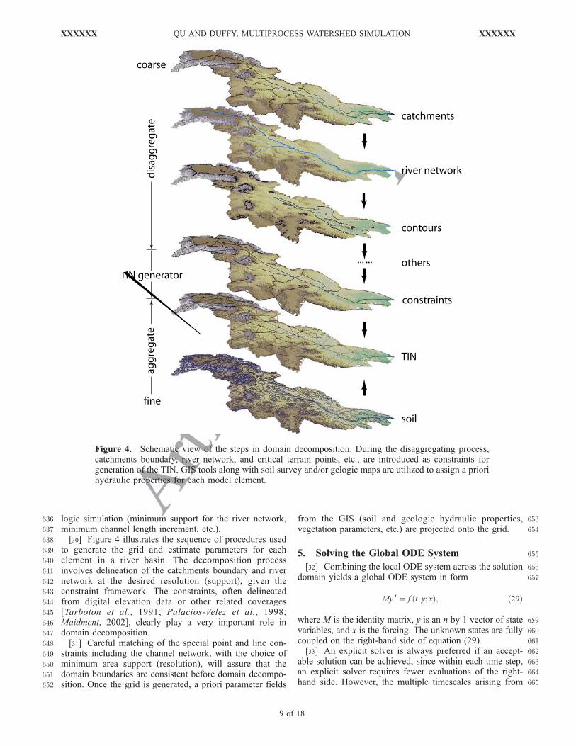
636 logic simulation (minimum support for the river network,637 minimum channel length increment, etc.).638 [30] Figure 4 illustrates the sequence of procedures used639 to generate the grid and estimate parameters for each640 element in a river basin. The decomposition process641 involves delineation of the catchments boundary and river642 network at the desired resolution (support), given the643 constraint framework. The constraints, often delineated644 from digital elevation data or other related coverages645 [Tarboton et al., 1991; Palacios-Velez et al., 1998;646 Maidment, 2002], clearly play a very important role in647 domain decomposition.648 [31] Careful matching of the special point and line con-649 straints including the channel network, with the choice of650 minimum area support (resolution), will assure that the651 domain boundaries are consistent before domain decompo-652 sition. Once the grid is generated, a priori parameter fields

653from the GIS (soil and geologic hydraulic properties,654vegetation parameters, etc.) are projected onto the grid.

6555. Solving the Global ODE System

656[32] Combining the local ODE system across the solution657domain yields a global ODE system in form

My 0 ¼ f t; y; xð Þ; ð29Þ

659where M is the identity matrix, y is an n by 1 vector of state660variables, and x is the forcing. The unknown states are fully661coupled on the right-hand side of equation (29).662[33] An explicit solver is always preferred if an accept-663able solution can be achieved, since within each time step,664an explicit solver requires fewer evaluations of the right-665hand side. However, the multiple timescales arising from

Figure 4. Schematic view of the steps in domain decomposition. During the disaggregating process,catchments boundary, river network, and critical terrain points, etc., are introduced as constraints forgeneration of the TIN. GIS tools along with soil survey and/or gelogic maps are utilized to assign a priorihydraulic properties for each model element.


9 of 18

XXXXXX

666 watershed processes typically make (29) a highly stiff667 system [Ascher and Petzold, 1998]. For stiff problems, the668 overall computational cost of an explicit solution may669 actually be higher than an implicit solver due to stability670 concerns. The implicit sequential solver used here is the671 SUNDIALS package (suite of nonlinear and differential/672 algebraic equation solvers), developed at the Lawrence673 Livermore National Laboratory. The code has been widely674 applied, with extensive testing, and with excellent support.675 [34] For the initial condition y(t0) = y0, a multistep676 formula is written

XK1i¼0

an;iyn�i þ hnXK2

i¼0

bn;iy0n�i ¼ 0; ð30Þ

678 where a and b are coefficients. For stiff ODEs, CVODE679 [Cohen and Hindmarsh, 1994] in the SUNDIAL package680 applies the backward differentiation formula (BDF) with681 an adaptive time step and method order varying between682 1 and 5. Applying (30) to (29) yields a nonlinear system683 of the form

G ynð Þ � yn � hnbn;0 f tn; ynð Þ � an ¼ 0 ð31Þ

684 with

an �Xi>0

an;iyn�i þ hnbn;iy0n�i

�: ð32Þ

687 Numerically solving equation (31), with some variant of688 Newton iteration, is equivalent to iteratively solving a689 linear system of the form

M yn mþ1ð Þ � yn mð Þ �

¼ �G yn mð Þ �

; ð33Þ

691 where M is I � hbn,0 J with J = @f/@y.

692[35] The GMRES (generalized minimal residual) iterative693linear solver in SUNDIAL makes the computational cost of694solving the global ODE system very competitive when695compared with other open-source solvers.

6966. The Shale Hills Field Experiment

697[36] The Shale Hills hydrologic experiment was con-698ducted on a 19.8-acre watershed in the Valley and Ridge699physiographic province of central Pennsylvania in 1974 by700the Forest Hydrology group at the Pennsylvania State701University [Lynch and Corbett, 1985; Lynch, 1976]. The702objectives of the experiment were to determine the physical703mechanisms of runoff and strea-flow generation at the704upland forested watershed, and to evaluate the effects of705antecedent soil moisture on the runoff peak and timing. The706fully coupled numerical model PIHM described earlier is707now applied to the Shale Hills site. The goal is to generally708explore the questions of the original field experiment using709an integrated model. Specifically these include the follow-710ing: (1) What is the impact of groundwater flow and soil711moisture on stream runoff and peakflow generation? (2)What

Figure 5. The Shale Hills watershed and measurement locations. It consists of 44 wells, 44 neutronprobes, and four weirs distributed over the 19-acre watershed.

Figure 6. Spray irrigation devices are regulated to controlthe rate of irrigation under the tree canopy during the ShaleHills experiment.

10 of 18


712 is the role of complex topography in producing runoff at713 Shale Hills? (3) Can fully coupled models improve the714 ability to simulate catchments that have ephemeral and/or715 intermittent channels?

717 6.1. Experimental Design and Data

718 [37] The design consisted of a comprehensive network of719 40 piezometers, 40 neutron access tubes for soil moisture,720 and four weirs. The distribution of sampling sites is shown721 in Figure 5. The upper part of the channel is ephemeral or722 intermittent, flowing during large storms or during the723 seasonal snowmelt period. The watershed was implemented724 with a spray irrigation network, shown in Figure 6, to725 precisely control the amount of artificial rainfall over the726 entire watershed. The irrigation was applied below the tree727 canopy and above forest litter, eliminating canopy intercep-728 tion storage during irrigation events. The watershed has a729 mixed deciduous and coniferous canopy, with a relatively730 thick forest litter. The soil profile at Shale Hills is typically a731 silt loam, ranging from 0.6-m thickness at the ridge top, to732 2.5 m deep near the channel. Three soil types are identified733 as Ashby, a shaley-silt loam in the upland portion of the734 watershed; the Blairton silt loam on the intermediate eleva-735 tion slopes; and the Ernest silt loam in the lower region736 along the channel. Underlying the soil is the Rose Hill Shale,737 which is thought to have a relatively low permeability738 [Lynch, 1976] and acts as an effective barrier to deeper flow.739 The bedrock topography was estimated by the limit of hand740 augering through the soil profile to bedrock.741 [38] From July to September 1974, a series of six equal742 artificial rainfall events (0.64 cm/h for 6 hours) were applied743 to the entire watershed [Lynch, 1976]. The events were744 timed such that the antecedent moisture gradually increased745 from very dry in the first storm, to near saturation after the

746last event. Along with the artificial rainfall, a few natural747rainfall events also occurred. We note that the experiment748was conducted in late summer through the fall season when749evapotranspiration is small, and when the snow and frost750could be neglected. Many irrigation treatments were con-751ducted during this experiment. The data chosen here spe-752cifically reflect an experiment to test the effect of antecedent753moisture on peak runoff by sequential storm events of the754same rate and duration.

7566.2. Water Budget

757[39] Figure 7 illustrates the forcing and runoff data mea-758sured at 15-min intervals from late July to early September.759Note the six artificial rainfall (irrigation) events, as well as760natural rainfall. Natural rainfall would of course be applied761to the top of the canopy. Nonetheless, during the late season762we assume interception storage to be small and can be763neglected.764[40] From the field data, the runoff/precipitation ratio is765calculated for each rainfall event and the results are given in766Table 1. A mass balance including change in storage shows

Figure 7. The six artificial rainfall events of equal magnitude and duration and the corresponding runoffat the outlet weir for the Shale Hills experiment.

t1.1Table 1. Observed Cumulative Input/Output and Runoff Ratio

for the 1974 Rainfall-Runoff Experiment at Shale Hills

Event DurationIrrigation,

mInput,m3

Output,m3

Runoff/PrecipitationRatio, % t1.2

1 1–7 Aug 0.04318 3355.236 407.4109 12.1 t1.32 7–14 Aug 0.045974 3572.339 998.8983 279 t1.43 14–19 Aug 0.038608 2999.975 1287.057 42.9 t1.54 19–23 Aug 0.038862 3019.712 1340.731 44.4 t1.65 23–27 Aug 0.04064 3157.869 1839.37 58.2 t1.76 27–31 Aug 0.071628 5565.744 3530.845 63.4 t1.8Total 1–31 Aug 0.2789 21670.88 9404.31 43.4 t1.9


11 of 18

XXXXXX

767 that 4.2% of total rainfall could not be accounted for in the768 balance. This ‘‘error’’ may be due to insufficient density of769 measurements, missing processes, or parameters (i.e., inter-770 ception or deep loss to bedrock).

772 6.3. Antecedent Soil Moisture Effect

773 [41] By conducting the experiment with equal rainfall774 events (0.64 cm/h for 6 hours), it is possible to test the effect775 of initial condition or antecedent moisture on runoff yield.776 We note that there was no significant infiltration-excess777 overland flow observed during the experiment. Apparently778 the infiltration capacity is large enough to accommodate the779 rainfall rate without producing overland flow. However, the780 deep forest litter makes this observation problematic.781 Figure 7 and Table 1 both indicate that as the antecedent782 moisture increases from a very dry to a very wet pre-event783 condition, the peak flow and total runoff increases as well,784 with only 12% of rainfall becoming runoff for the first storm785 (very dry), and 63% runoff ratio for very wet conditions.786 The relaxation for the sixth event in Figure 7 and the runoff787 ratio in Table 1 clearly suggest the significance of soil788 moisture and groundwater storage on the changing moisture789 threshold for rainfall-runoff generation. This is examined in790 more detail with the integrated model implementation next.

792 6.4. Model Domain and a Priori Data

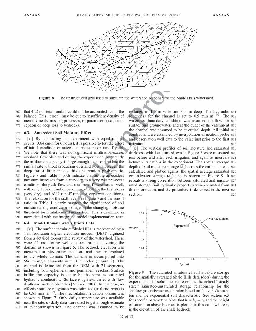
793 [42] The surface terrain at Shale Hills is represented by a794 1-m resolution digital elevation modedl (DEM) digitized795 from a detailed topographic survey of the watershed. There796 were 44 monitoring wells/neutron probes covering the797 domain as shown in Figure 5. The bedrock elevation was798 measured at piezometer locations and then interpolated799 to the whole domain. The domain is decomposed into800 566 triangle elements with 315 nodes (Figure 8). The801 channel is delineated from the DEM with 21 segments,802 including both ephemeral and permanent reaches. Surface803 infiltration capacity is set to be the same as saturated804 hydraulic conductivity. Surface roughness varies with flow

depth and surface obstacles [Hauser, 2003]. In this case, an806 effective surface roughness was estimated (trial and error) to807 be 0.83 min m�1/3. The precipitation/irrigation forcing was808 shown in Figure 7. Only daily temperature was available809 near the site, so daily data were used to get a rough estimate810 of evapotranspiration. The channel was assumed to be

811rectangular, 1.5 m wide and 0.5 m deep. The hydraulic812roughness for the channel is set to 0.5 min m�1/3. The813watershed boundary condition was assumed no flow for814surface and groundwater, and at the outlet of the catchment815the channel was assumed to be at critical depth. All initial816conditions were estimated by interpolation of neutron probe817and observation well data to the value just prior to the first818irrigation.819[43] The vertical profiles of soil moisture and saturated820thickness with locations shown in Figure 5 were measured821just before and after each irrigation and again at intervals822between irrigations in the experiment. The spatial average823depth of soil moisture storage (hu) across the entire site was824calculated and plotted against the spatial average saturated825groundwater storage (hg) and is shown in Figure 9. It826reveals a strong correlation between saturated and unsatu-827rated storage. Soil hydraulic properties were estimated from828this information, and the procedure is described in the next829section.

Figure 9. The saturated-unsaturated soil moisture storagefor the spatially averaged Shale Hills data (dots) during theexperiment. The solid lines represent the theoretical ‘‘steadystate’’ saturated-unsaturated storage relationship for theshallow groundwater assumption based on the van Genuch-ten and the exponential soil characteristic. See section 6.5for specific parameters. Note that hs = hg � zb and the heightof saturation above bedrock is plotted in this case, where zbis the elevation of the shale bedrock.

Figure 8. The unstructured grid used to simulate the watershed response for the Shale Hills watershed.

12 of 18


8316.5. Simpified Shale Hills Model

832[44] The system of equations developed in section 3 was833used to model the Shale Hills site. However, it was834determined that a simplification was possible as a result835of the shallow soil at the site. Duffy [2004] developed a836theoretical argument, that where the groundwater table is837near the land surface, the governing equations for subsur-838face flow can be simplified into a single state by applying839the ‘‘enslaving principal.’’ That is, the water table enslaves840the soil moisture such that

dhu

dt¼ G hg

� dhgdt

ð34Þ

G hg �

¼ dhu

dhg; ð35Þ

844where G(hg) can be thought of as the integrated form of the845soil characteristic function (see Duffy [2004] for details).846This argument is essentially what was done by Bierkens847[1998] in an earlier paper. The coupled two-state subsurface848model (20) can now be reduced to

G hg � dhg

dt¼ pþ qþ � et þ

X3j¼1

qgj : ð36Þ

Figure 10. Observed and model groundwater levels for1 August, 16 August, and 29 August. The fit is notsignificantly different from a slope of 1.

Figure 11. Observed (blue) versus model (red) runoff simulation for Shale Hills experiment. Note thatthe coupled model successfully simulates the internal runoff at each weir, including the upper ephemeralpart of the channel.


13 of 18

XXXXXX

850 Bierkens [1998] uses the van Genuchten soil characteristic851 function to derive a form for G(hg) in (34) given by

G hg �

¼ e0 þ qs � qrð Þ 1� 1þ a zs � hð Þð Þnð Þ� nþ1ð Þ=nð Þ�

; ð37Þ

853 where hg and zs are height of phreatic surface and surface854 elevation of the layer relative to some reference. The e0 is a855 small parameter to handle the singularity in the function856 G(hg)

�1 when hg ! zs. The qs and qr are saturated and857 residual moisture content, and a and n are soil parameters.858 Substituting (18) and (35) into (37), and performing the859 integration yields an expression for hu as a function of hg:

hu ¼1

a1þ a zs � hg

� ��n� ��1n: ð38Þ

861A similar expression can be developed for the exponential862soil characteristic (22) shown earlier which is given by

hu ¼1

a1� e�a zx�hgð Þ�

: ð39Þ

864Using the site averaged data for hu and hg, the parameters in865(38) and (39) were estimated and the results shown in866Figure 9. The mean data from Figure 9 were used together867with the soil survey information to estimate van Genuchten868parameters used in the simulation: qs = 0.40, qr = 0.05, a =8692.0 L/m, n = 1.8, 0.6 � zs � 2.5 m, and Ks = 1 � 10�5 m/s.870Also note in Figure 9 that the height of saturation above the871shale bedrock elevation is plotted using hs = hg � zb.

8736.6. Model Results

874[45] For the domain, forcing, and a priori parameters875described above, the simulation was carried out on a dual-876processor desktop machine, completing the simulation in a

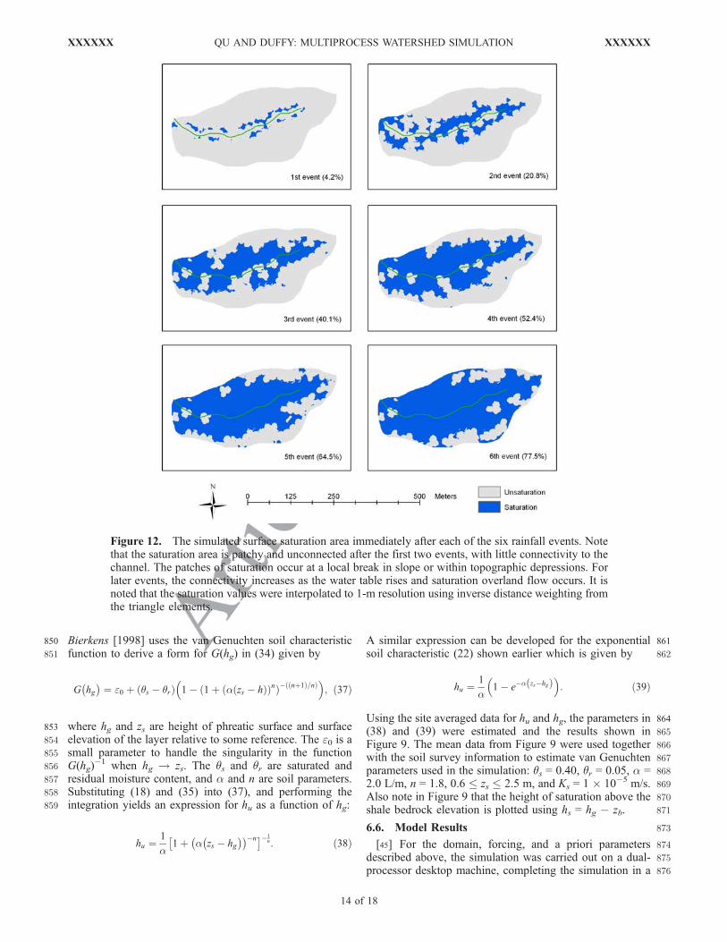
Figure 12. The simulated surface saturation area immediately after each of the six rainfall events. Notethat the saturation area is patchy and unconnected after the first two events, with little connectivity to thechannel. The patches of saturation occur at a local break in slope or within topographic depressions. Forlater events, the connectivity increases as the water table rises and saturation overland flow occurs. It isnoted that the saturation values were interpolated to 1-m resolution using inverse distance weighting fromthe triangle elements.

14 of 18


877 few seconds. Because of the relatively small scale of the878 simulation, computational efficiency is not an issue in this879 problem. Figure 10 compares modeled and observed880 groundwater depth for three days during the experiment,881 1 August, 16 August, and 30 August, respectively, with an882 overall regression slope of 1.05, and R = 0.965. Figure 11883 illustrates simulated and observed runoff data at all four884 weirs. The first event does not match as well as others,885 due possibly to errors in the initial conditions, and this is886 discussed below. The sixth event also shows some depar-887 ture, which might be related to our assumption to neglect888 canopy interception. It is interesting that both the obser-889 vations and the model display a double peak in the890 hydrograph for each single rainfall event (Figure 11). This891 seems to be caused by a complex interaction of surface892 runoff controlled by small-scale topography and near-893 channel surface runoff, with subsurface flow. Additional894 experiments are necessary to partition the precise effects,895 but it is clear that the fully coupled distributed model can896 capture this kind of behavior. For the Shale Hills field897 experiment the rainfall-runoff generation mechanisms as-898 sumed in the model include Hortonian overland flow due899 to precipitation excess, and saturation overland flow. During900 most of the numerical experiment, the soil infiltration capac-901 ity is large enough to accommodate rainfall, and Hortonian902 flow is of limited importance except in the upland regions903 during the fifth and sixth events. Saturation overland flow904 occurs at locations where water table saturates the land905 surface from below. In Figure 12, the simulated regions of906 surface saturation after each rainfall event are plotted. Note907 that the saturation area is patchy and unconnected during the908 first two events with little connectivity to the channel. The909 patches of saturation occur at a local break in slope or in

910topographic depressions. Recall that the hydraulic properties911of the soil and the forcing in the watershed are homogeneous,912and thus local variability is largely the result of topography.913The impact of noncontiguous temporary patches of saturation914is that the water reinfiltrates locally since it does not have a915path to the channel. This threshold for surface flow due to916local topography is discussed by VanderKwaak and Loague917[2001], and they introduce a subgrid parameterization to918resolve it.919[46] For later rainfall events (3–6), the connectivity of920surface saturation increases as the water table rises and921saturation overland flow connects the patches with the922channel. Rejected rainfall during the later events also923contributes to an increase in saturated area. In this analysis,924the surface and bedrock topography exert a strong control925on saturation overland flow, and thus have a dominant926impact on surface runoff in Shale Hills experiment. This927is similar to observations of Amerman [1965] and Dunne928and Black [1970a, 1970b] at other northeastern watersheds.929[47] Another aspect of the simulation observed in930Figure 11 is the onset of streamflow in the upper ephemeral931channel reach. Channel flow in the upper part of the932watershed is only observed during years with heavy snow933or after very large fall storms. Figure 13 shows the inte-934grated model result for flow depth along the channel in935response to the third rainfall event. The beginning of the936third rainfall is identified as 0 min and most of the channel937is dry (not shown). During the event (200 min) the length of938flowing channel has grown considerably. After 400 min the939event is over, and the channel continues to grow until about94010 hours, when it reaches a maximum and begins to relax.941After 3000 min the channel reach is largely dry again. The942ability to examine the internal details of the flow is an

Figure 13. The flow depth along the channel for the third irrigation event. The solid lines show thedistribution of flow depth during the event and immediately after the event (600 min). The dashed linesshow the flow depth during the relaxation or recession period. The outlet weir is located on the right sideof the graph.


15 of 18

XXXXXX

943 important aspect of the fully coupled approach, including944 thresholds of wet and dry channels.

946 6.7. Sensitivity to Initial Conditions

947 [48] Next we simulate the impact of very dry antecedent948 soil moisture and low water table conditions to get some949 idea of the time it takes the watershed to recover from a950 major drought. The model is run with the same forcing951 sequence except that the initial states (groundwater and soil952 moisture) are reduced to the minimum possible values. The953 response at the outlet weir is shown in Figure 14. Note that954 it takes a relatively short time for a complete recovery of955 peak flow as compared with the previous simulation (third956 event or 333 hours). This simple result offers a clue that957 there is some problem with our assumptions in the model,958 since it has been subsequently observed during the 1990’s959 drought, that the outlet weir completely dried up and did not960 recover for several years. This suggests that there might be a961 slower and deeper flow component (e.g., a multiyear962 timescale) within the underlying less permeable shale rego-963 lith. This might also explain the missing mass described964 earlier, and this study is currently under way.

966 7. Conclusions

967 [49] In this paper we describe a semidiscrete finite vol-968 ume strategy for fully coupled integrated hydrologic model969 that is efficient for adding and subtracting processes and for970 constructing the discrete solution domain. We demonstrate

971the strategy by coupling equations for a mixed PDE-ODE972system that includes 2-D overland flow, 1-D channel flow,9731-D unsaturated flow, and 2-D groundwater flow, canopy974interception, and snowmelt. The complete system of equa-975tions including constitutive or closure relations is coupled976directly within a local kernel for a single prismatic element.977GIS tools are used to decompose the domain into an978unstructured grid, and the kernel is distributed over the grid979and assembled to form the global ODE system. The global980ODE system is solved with a state-of-the-art ODE solver.981The strategy provides an efficient and flexible way to982couple multiple distributed processes that can capture983detailed dynamics with a minimum of elements. The FVM984guarantees mass conservation during simulation at all cells.985The model is referred to as the Penn State Integrated986Hydrologic Model (PIHM).987[50] The approach has been implemented at the Shale988Hills field experiment in central Pennsylvania. Model989results show that it can successfully simulate observed990groundwater levels, as well as runoff at the outlet and at991internal points within the watershed using a priori param-992eters. The simulation is used to identify the important runoff993generation mechanisms, and to illustrate the impact of994antecedent soil moisture and groundwater level for ampli-995fying the volume and peak runoff in the watershed. The996effect of complex topography is shown to be a very997important control on infiltration/reinfiltration areas within998the watershed. The coupled model is able to simulate the

Figure 14. Simulation of the effect of a dry initial condition (drought persistence) on runoff at theoutlet. The initial condition for soil moisture and groundwater level was set to very low values and thenthe experimental forcing was applied to the model. Note that the recovery is complete at approximately333 hours.

16 of 18


999 onset and relaxation of ephemeral streamflow in the upland1000 part of the watershed. The processes and components of the1001 model have been individually tested, and these results are1002 given by Qu [2005]. A complete GIS interface for PIHM is1003 currently being finalized for Web posting as a flexible and1004 easily implemented open-source community modeling1005 resource.

1006 [51] Acknowledgments. This research was funded by grants from the1007 National Science Foundation (Science and Technology Center for Sustain-1008 ability of Water Resources in Semi-Arid Regions, NSF EAR 9876800;1009 Integrated modeling of precipitation-recharge-runoff at the river basin scale:1010 The Susquehanna, NSF ER030030), the National Oceanic and Atmospheric1011 Administration (Modeling seasonal to decadal oscillations in closed basins,1012 NOAA_GAPP Program, NA04OAR4310085), and the National Aeronau-1013 tics and Space Administration (The role of soil moisture and water table1014 dynamics in ungaged runoff prediction in mountain-front systems, NASA_1015 GAPP Program, ER020059). This support is kindly acknowledged.

1016 References1017 Abbott, M. B., J. A. Bathurst, and P. E. Cunge (1986a), An introduction to1018 the European Hydrological System–Systeme Hydrologicque Europeen1019 ‘‘SHE’’: part 1. History and philosophy of a physically based distributed1020 modeling system, J. Hydrol., 87, 45–59.1021 Abbott, M. B., J. A. Bathurst, and P. E. Cunge (1986b), An introduction to1022 the European Hydrological System–Systeme Hydrologicque Europeen1023 ‘‘SHE’’: part 2. Structure of a physically based distributed modeling1024 system, J. Hydrol., 87, 61–77.1025 Allen, R. G., L. S. Pereira, D. Raes, and M. Smith (1998), Crop evapo-1026 transpiration, FAO Irrig. Drain. Pap. 56, United Nations Food and Agric.1027 Organ., Rome.1028 Amerman, C. R. (1965), The use of unit-source watershed data for runoff1029 prediction, Water Resour. Res., 1(4), 499–508.1030 Ascher, U. M., and L. R. Petzold (1998), Computer Methods for Ordinary1031 Differential Equations and Differential Algebraic Equations, Soc. for1032 Ind. and Appl. Math., Philadelphia, Pa.1033 Beven, K. (2006), Searching for the holy grail of scientific hydrology: Qt =1034 H(SR)A as closure, Hydrol. Earth Syst. Sci. Discuss., 3, 769–792.1035 Bierkens, M. F. P. (1998), Modeling water table fluctuations by means of a1036 stochastic differential equation, Water Resour. Res., 34(10), 2485–2499.1037 Brandes, D. (1998), A low-dimensional dynamical model of hillslope soil1038 moisture, with application to a semiarid field site, Ph.D. thesis, Pa. State1039 Univ., University Park.1040 Bras, R. L. (1990), Hydrology: An Introduction to Hydrologic Science,1041 Addison-Wesley, Boston, Mass.1042 Brooks, R. H., and A. T. Corey (1964), Hydraulic properties of porous1043 media, Hydrol. Pap. 3, Colo. State Univ., Fort Collins.1044 Cohen, S. D., and A. C. Hindmarsh (1994), CVODE user guide, Rep.1045 UCRL-MA-118618, Numer. Math. Group, Lawrence Livermore Natl.1046 Lab., Livermore, Calif.1047 Crawford, N. H., and R. K. Linsley (1966), Digital simulation on hydrology:1048 Stanford Watershed Model IV, Stanford Univ. Tech. Rep. 39, Stanford1049 Univ., Palo Alto, Calif.1050 Delanunay, B. (1934), Sur la sphere vide, Bull. Acad. Sci. USSR Class Sci.1051 Math. Nat., 7(6), 793–800.1052 Dingman, S. L. (1994), Physical Hydrology, Prentice-Hall, Upper Saddle1053 River, N. J.1054 Du, Q., V. Faber, and M. Gunzburger (1999), Centroidal Voronoi tessala-1055 tions: Applications and algorithms, SIAM Rev., 41(4), 637–676.1056 Duffy, C. J. (1996), A two-state integral-balance model for soil moisture1057 and groundwater dynamics in complex terrain,Water Resour. Res., 32(8),1058 2421–2434.1059 Duffy, C. J. (2004), Semi-discrete dynamical model for mountain-front1060 recharge and water balance estimation, Rio Grande of southern Colorado1061 and New Mexico, in Groundwater Recharge in a Desert Environment:1062 The Southwestern United States, Water Sci. Appl. Ser., vol. 9, edited by1063 J. F. Hogan et al., pp. 255–271, AGU, Washington, D. C.1064 Dunne, T., and R. D. Black (1970a), An experimental investigation of1065 runoff production in permeable soils,Water Resour. Res., 6(2), 478–490.1066 Dunne, T., and R. D. Black (1970b), Partial area contributions to storm1067 runoff in a small New England watershed, Water Resour. Res., 6(5),1068 1296–1311.1069 Freeze, R. A., and R. L. Harlan (1969), Blueprint for a physically-based,1070 digitally-simulated hydrologic response model, J. Hydrol., 9, 237–258.

1071Gardner, W. R. (1958), Some steady-state solutions of the unsaturated1072moisture flow equation with application to evaporation from a water1073table, Soil Sci., 85, 228–232.1074Gottardi, G., and M. Venutelli (1993), A control-volume finite-element1075model for two-dimensional overland flow, Adv. Water Resour., 16,1076277–284.1077Hauser, G. E. (2003), River modeling system user guide and technical1078reference, report, Tenn. Valley Auth., Norris, Tenn.1079Kristensen, K. J., and S. E. Jensen (1975), A model for estimating actual1080evapotranspiration from potential evapotranspiration, Nord. Hydrol., 6,1081170–188.1082LaBolle, E. M., A. A. Ayman, and E. F. Graham (2003), Review of the1083integrated groundwater and surface-water model (IGSM), Ground Water,108441(2), 238–246.1085Leveque, R. J. (2002), Finite Volume Methods for Hyperbolic Problems,1086Cambridge Univ. Press, New York.1087Lynch, J. A. (1976), Effects of antecedent moisture on storage hydrographs,1088Ph.D. thesis, 192 pp., Dep. of Forestry, Pa. State Univ., University Park.1089Lynch, J. A., andW. Corbett (1985), Source-area variability during peakflow,1090in watershed management in the 80’s, J. Irrig. Drain. Eng., 300–307.1091Madsen, N. K. (1975), The method of lines for the numerical solution of1092partial differential equations, in Proceedings of the SIGNUM Meeting on1093Software for Partial Differential Equations, pp. 5–7, ACM Press, New1094York.1095Maidment, D. R. (2002), Arc Hydro: GIS for Water Resources, 140 pp.,1096ESRI Press, Redlands, Calif.1097Palacios-Velez, O. L., and B. Duevas-Renaud (1986), Automated river-1098course, ridge and basin delineation from digital elevation data, J. Hydrol.,109986, 299–314.1100Palacios-Velez, O., W. Gandoy-Bernasconi, and B. Cuevas-Renaud (1998),1101Geometric analysis of surface runoff and the computation order of unit1102elements in distributed hydrological models, J. Hydrol., 211, 266–274.1103Panday, S., and P. S. Huyakorn (2004), A fully coupled physically-based1104spatially-distributed model for evaluating surface/subsurface flow, Adv.1105Water Resour., 27, 361–382.1106Polis, M. F., and D. M. McKeown (1993), Issues in iterative TIN generation1107to support large scale simulations, paper presented at 11th International1108Symposium on Computer Assisted Cartography (AUTOCARTO11),1109Minneapolis, Minn.1110Post, D. E., and L. G. Votta (2005), Computational science demands a new1111paradigm, Phys. Today, 58(1), 35–41.1112Qu, Y. (2005), An integrated hydrologic model for multi-process simulation1113using semi-discrete finite volume approach, Ph.D. thesis, 136 pp., Civ.1114and Environ. Eng. Dep., Pa. State Univ., Univ. Park.1115Reggiani, P., and T. H. M. Rientjes (2005), Flux parameterization in the1116representative elementary watershed approach: Application to a natural1117basin, Water Resour. Res., 41, W04013, doi:10.1029/2004WR003693.1118Reggiani, P., M. Sivapalan, and M. Hassanizadeh (1998), A unifying frame-1119work for watershed thermodynamics: Balance equations for mass,1120momentum, energy and entropy, and the second law of thermodynamics,1121Adv. Water Res., 22, 367–398.1122Reggiani, P., M. Hassanizadeh, M. Sivapalan, and W. G. Gray (1999), A1123unifying framework for watershed thermodynamics: Constitutive rela-1124tionships, Adv. Water Res., 23, 15–39.1125Shewchuk, J. R. (1997), Delaunay refinement mesh generation, Ph.D.1126thesis, Carnegie Mellon Univ., Pittsburgh, Pa.1127Sivapalan, M., C. Jothityangkoon, and M. Menabde (2002), Linearity and1128non-linearity of basin response as a function of scale: Discussion of1129alternative definitions, Water Resour. Res., 38(2), 1012, doi:10.1029/11302001WR000482.1131Slattery, J. (1978), Momentum, Energy, and Mass Transfer in Continua,1132Krieger, Melbourne, Fla.1133Sleigh, P. A., P. H. Gaskell, M. Berzins, and N. G. Wright (1998), An1134unstructured finite-volume algorithm for predicting flow in rivers and1135estuaries, Comput. Fluids, 27(4), 479–508.1136Tarboton, D. G., R. L. Bras, and I. Rodriguez-Iturbe (1991), On the extrac-1137tion of channel networks from digital elevation data, Hydrol. Processes,11385, 81–100.1139VanderKwaak, J. E., and K. Loague (2001), Hydrologic response simula-1140tions for the R-5 catchment with a comprehensive physics-based model,1141Water Resour. Res., 37(4), 999–1013.1142van Genuchten, M. T. (1980), A closed form equation for predicting the1143hydraulic conductivity of unsaturated soils, Soil Sci. Soc. Am. J., 44,1144892–898.1145Vivoni, E. R., V. Y. Ivanov, R. L. Bras, and D. Entekhabi (2004), Genera-1146tion of triangulated irregular networks based on hydrological similarity,1147J. Hydrol. Eng., 9(4), 288–302.


17 of 18

XXXXXX

1148 Voronoi, G. (1907), Nouvelles applications des parametres continus a la1149 theorie des formes quadratiques, J. Reine Angewandte Math., 133, 97–1150 178.1151 Yeh, G. T., H. P. Cheng, J. R. Cheng, H. C. Lin, and W. D. Martin (1998), A1152 numerical model simulating water flow, contaminant and sediment trans-1153 port in a watershed systems of 1-D stream-river network, 2-D overland

1154regime, and 3-D subsurface media (WASH123D: Version 1.0), Tech.1155Rep. CHL-98-19, U. S. Environ. Prot. Agency Environ. Res. Lab.,1156Athens, Ga.

��1158C. Duffy and Y. Qu, Department of Civil and Environmental1159Engineering, Pennsylvania State University, 212 Sackett Building,1160University Park, PA 16802, USA. ([email protected])

18 of 18


click here full article a semidiscrete finite volume

Documents