Classification of Legendrian Knots and Links

Wutichai Chongchitmate

April 28, 2010

1 Introduction

The aim of this paper is to use computer program to generate and classify Legendrianknots and links. Modifying the algorithm in [11], we write a program in Java to generateall grid diagrams of up to size 10. Since classification of Legendrian links up to Legendrianisotopy is equivalent to grid diagrams modulo a set of Cromwell moves including translation,commutation and 𝑋:NE,𝑋:SW (de)stabilization [17], we can identify two grid diagrams andcheck whether they represent the same Legendrian link.

We also use various topological, Legendrian and transverse invariants for knots andlinks to distinguish Legendrian knots and links generated by the algorithm. Since classicalLegendrian invariants are not enough for classification, we use several non-classical ones suchas graded ruling invariant and linearized contact homology. To refine our result even further,we use several techniques such as the Chekanov-Eliashberg differential graded algebra (DGA)[13] and knot Floer homology [15].

The main result of this paper consists of two atlases, a Legendrian knot atlas (table 1)and an atlas for unoriented Legendrian two-component links (table 3). We also provide atransverse knot atlas (table 2), which can be inferred from the Legendrian knot atlas. In theLegendrian knot atlas, we give information on grid diagram, Thurston-Bennequin number,rotation number, polynomials for graded ruling invariant and linearized contact homologyfor each Legendrian knot with knot type of arc index up to 9. For each knot type, we alsoprovide conjecture for its mountain range.

The Legendrian knot atlas also illustrates several interesting phenomena such as unusualmountain ranges for 10161, 𝑚(10139) and 𝑚(12𝑛242), and transversely non-simple knots for𝑚(10145), 𝑚(10161) and 12𝑛591. The later group is depicted in their mountain ranges asLegendrian knots whose Thurston-Bennequin number is not equal to the maximal Thurston-Bennequin number of their knot type but are not stabilization of any Legendrian knots. Priorto this paper, such phenomenon was found only in knots with very large number of crossings.

The atlas for unoriented Legendrian two-component links also gives information on griddiagram, Thurston-Bennequin number and rotation number for each unoriented Legendrianlink with link type of arc index up to 9. We also give information on whether its twocomponents can be switched via topological isotopy and conjecture on whether they can

1

be switched via Legendrian isotopy. For each link type, we also provide conjecture for itsThurston-Bennequin polytope [1]. Our result can answer the question posted by Baaderand Ishikawa in [1] that whether the tb polytope can always be described by the three linearinequalities.

2 Knots and Links

In mathematics, a knot is a simple closed curve in 3-dimensional Euclidean space, ℝ3. Onecan simply think of knot as one piece of string with its ends glued together. Formally, wecan define a knot as follows.

Definition 1. A knot is a smooth embedding 𝐾 : 𝑆1 → ℝ3. Two knots are equivalent (or

topological isotopic) if they are ambient isotopic.

In other word, two knots are equivalent if one can continuously deform to the otherwithout brreaking or intersecting itself. We call an equivalence class of knots a knot type.Some simpler knot types are well-studied and have names such as “trefoil knot” and “thefigure-eight knot”.

We usually represent knots by their immersion on ℝ2 such that the restriction map

𝑆1 → ℝ2 is injective except finite number of points, in which case the map is two-to-one

and transverse, i.e., tangent lines should not coincide at the crossing. Such a projection iscalled knot diagram. The two-to-one points are called crossings. At each crossing, we needto specify which strand passes over or in front of another strand. We call the strand thatpasses over overstrand and another understrand. Distinct knot diagrams can represent knotswith the same knot type. We can define crossing number of a particular knot type to be theminimum number of crossings of any knot diagrams representing that knot type.

The main problem in knot theory is to classify knots and decide whether two given knotsare equivalent. Traditionally, knots are classified by crossing numbers and hence we have aknot table as in Figure 1. Each knot type is labeled as 𝐶𝑖 where 𝐶 is the crossing numberand 𝑖 is an index within the knots of the same crossing number. For example, the trefoil knotis labeled 31. The standard knot table with such labeled for all prime knots with less than11 crossings is called the Rolfsen knot table. For knots with 11 crossings or more, we furthercategorize them by whether a knot is alternating, i.e., whether the crossings alternate under,over, under, over, as one travels along the strand. Otherwise, a knot is non-alternating. Wethen labeled an alternating knot by 𝐶𝑎𝑖 and a non-alternating knot by 𝐶𝑛𝑖. The standardknot table for knots with 11 crossing is called the Hoste-Thistlethwaite table. The largestknot table consists of all knots with up to 16 crossings.

It is not simple to show the equivalence of two given knots by using only the definition.In 1926, Kurt Reidemeister, and independently, in 1927, J.W. Alexander and G.B. Briggsproved that two knot diagrams represent knots with the same knot type if and only if onecan be transformed to the other via planar isotopy by a sequence of three kinds of moves,

2

Figure 1: Knot Table 1

called Reidemeister moves as shown in Figure 2.

(a) Type I (b) Type II

(c) Type III

Figure 2: Reidemeister Moves 2

1http://en.wikipedia.org/wiki/Knot (mathematics)

3

Although Reidemeister moves provide more convenient and systematic way to showequivalence of two knot diagrams, they does not give a deterministic algorithm to clas-sify knots. In general, we do not know how many moves we need to use to transform oneknot diagram to the other. Hence, it is not possible to use Reidemeister moves to distinguishtwo knot diagrams that possibly belong to different knot types.

Sometimes we give an orientation to knot, denoted by arrows in knot diagram as inFigure 3. Two knots of the same knot diagram but different orientation may or may notbe equivalent. A mirror image of a knot, which can be obtained by reversing all crossings,may or may not be equivalent to the original one. The mirror image of a knot 𝐾 usuallydenoted by 𝑚(𝐾) or 𝐾.

Figure 3: Two Orientations of Trefoil Knot 3

We can assign some “value” such as integer, polynomial or even algebraic structure, toeach knot. If the values is invariant under three types of Reidermester moves, we call suchvalues knot invariants. Clearly, crossing number is a knot invariant by definition. Someknot invariants is defined in a way that one can determine such value from knot diagram.We may use these knot invariants to show that two diagrams represent different knot type.

For oriented knot, we call a crossing positive if one can turn the direction of the overstrandcounterclockwise to match the direction of the understrand with the angle less than a half-turn. Otherwise, we call a crossing negative (Figure 4). For each crossing 𝑐, we may define

𝜖(𝑐) =

{1 𝑐 positive−1 𝑐 negative

Then the writhe of a diagram 𝐷 is

𝑤𝑟(𝐷) =∑

crossing 𝑐 in 𝐷

𝜖(𝑐).

Although writhe is not a knot invariant as it is not invariant under Reidemeister I move, itis useful quatity that we will use to compute several invariants later in this paper.

2http://en.wikipedia.org/wiki/Knot theory3http://www.math.cornell.edu/˜mec/2008-2009/HoHonLeung/page2 knots.htm

4

(a) positive crossing (b) negative crossing

Figure 4: Positive and Negative Crossings4

We can also consider a union of disjoint embeddings of 𝑆1 in ℝ3. We call a collection of

disjoint knots a link. Two links are equivalent (or topological isotopic) if they are ambientisotopic. Each embedding of 𝑆1 is called a component of a link. A knot is simply a linkwith one component. Most results for knots apply to links as well. For example, two linkdiagrams represent links with the same link type if and only if one can be transformed to theother by a sequence of Reidemeister moves. Note that if we consider only one componentof a link and omit the rest, it will become a knot. We can also construct a link from a knotto get some extra properties and invariants, which we will discuss later on in this paper.Hence, the study of knots and links are strongly related.

The concept of invariants also applies to links. Several knot invariants are also linkinvariant. In addition, there are several link invariants that are only useful to links withmore than one component. For example, the linking number of components 𝐿1 and 𝐿2 of alink 𝐿 is

𝑙𝑘(𝐿1, 𝐿2) =1

2

∑crossing 𝑐 between 𝐿1 and 𝐿2

𝜖(𝑐).

In other word, the linking number is half of the total number of positive crossings betweencomponents minus the total number of negative crossings between components. We can seethat the linking number of any diagram is always an integer, and the linking number is aninvariant of a link with two components.

Several other useful and widely used knot and link invariants are Kauffman polyno-mial, Jones polynomial, HOMFLY-PT polynomial and Alexander polynomial. We shall notdiscuss the meaning of these invariants in detail. Given some representation of knot andMathematica can compute these invariants if the knot is not too large.

Similar to knots, links are traditionally classified by their crossing numbers. Links arealso considered whether they are alternating or non-alternating. A link is labeled 𝐿𝑐𝑎𝑖 and𝐿𝑐𝑛𝑖, respectively, where 𝑐 is its crossing number and 𝑖 is an index within (non-)alternating

4http://en.wikipedia.org/wiki/Writhe5http://en.wikipedia.org/wiki/Linking number

5

Figure 5: A Two-Component Link with Linking Number Two5

knots of the same crossing number (Figure 6). Unlike knots, links are less studied and morecomplicated. The Thistlethwaite link table consists of all prime links with up to 13 crossings.

Figure 6: Link Table6

3 Legendrian and Transverse Knots

Definition 2. Let 𝐿 be a knot parametrized by a map 𝑆1 → ℝ3 defined by

𝜃 �→ (𝑥(𝜃), 𝑦(𝜃), 𝑧(𝜃)).

Then 𝐿 is a Legendrian knot if

𝑧′(𝜃)− 𝑦(𝜃)𝑥′(𝜃) = 0.

There are several ways to represent or project a Legendrian knot in ℝ2. Throughout

this paper, we shall use a front projection defined by the map Π : ℝ3 → ℝ2 which sends

(𝑥, 𝑦, 𝑧) �→ (𝑥, 𝑧). Since 𝑧′(𝜃) − 𝑦(𝜃)𝑥′(𝜃) = 0, we can retrieve 𝑦(𝜃) from 𝑥(𝜃) and 𝑧(𝜃) by

𝑦(𝜃) = 𝑧′(𝜃)𝑥′(𝜃) = 𝑑𝑧

𝑑𝑥 . We call an image of the projection at 𝑥′(𝜃) = 0 a cusp. The image offront projection, called Legendrian front diagram or front diagram, is a knot diagram withthe following properties:

6http://katlas.math.toronto.edu/wiki/The Thistlethwaite Link Table

6

1. has no vertical tengencies

2. the only non-smooth points are horizontal cusps

3. at each crossing, the slope of the overcrossing strand is smaller (more negative) thanthe undercrossing strand.

Moreover, any knot diagram satisfying all of the above three properties is a front diagramof a Legendrian knot. The third property allows us to omit the notation indicating whichstrand is overcrossing at each crossing. We can write front diagrams as in Figure 7.

Figure 7: Front Diagrams of unknot, trefoil knot and the figure-eight knot

Similar to topological knot, two Legendrian knots are equivalent or Legendrian isotopic ifthey are ambient isotopic in the way that a knot at every state of deformation is Legendrian.Figure 8 shows three types of Legendrian Reidemeister moves on a front diagram which areanalogous to Reidemeister moves for topological knots on a knot diagram. The result ofSwiatkowski [19] shows that two front diagrams represent equivalent Legendrian knots ifand only if they relate by a sequence of Legendrian Reidemeister moves.

Clearly, a Legendrian knot is also a topological knot. One may consider a front diagramas a knot diagram. Legendrian isotopy is also a topological isotopy, but not the other wayaround. For any topological knot type, there are Legendrian knots representing it. One canconstruct a Legendrian knot, or, in particular, its front diagram, from a knot diagram byadding cusps and zig-zags as shown in Figure 9.

We can view Legendrian knots as subtypes of topological knots. Each topological knotbelongs to exactly one knot type. Hence, topological knot type is an invariant of Legen-drian knots. In fact, it is one of three classical Legendrian invariants which are the mostfundamental tools to classify Legendrian knots throughout this paper. We shall denote thetopological type of a Legendrian knot 𝐿 by 𝑘(𝐿).

Another classical Legendrian invariant is the Thurston-Bennequin number, denoted by𝑡𝑏, or 𝑡𝑏(𝐿) for the Thurston-Bennequin number of a Legendrian knot 𝐿. The Thurston-Bennequin number is defined in several ways, but for our convenience, we shall define it

7

Figure 8: Legendrian Reidemeister Moves [7]

combinatorially from a front diagram. Let 𝑐(𝐷) be the number of left cusps in a frontdiagram 𝐷. Note that in any front diagram, the number of left cusps is equal to the numberof right cusps. Thus, 𝑐(𝐷) is also half of the number of all cusps in 𝐷. The Thurston-Bennequin number of a Legendrian knot 𝐿 with a front diagram 𝐷 is

𝑡𝑏(𝐿) = 𝑤𝑟(𝐷)− 𝑐(𝐷).

The last classical Legendrian invariant is the rotation number, denoted by 𝑟, or 𝑟(𝐿) forthe rotation number of an oriented Legendrian knot 𝐿. We may define the rotation numbercombinatorially as follows. For an oriented front diagram 𝐷, let 𝑐↓(𝐷) be the total numberof downward cusps in 𝐷 and 𝑐↑(𝐷) be the total number of upward cusps in 𝐷 (Figure 10).Then the rotation number of 𝐿 represented by 𝐷 is

𝑟(𝐿) =1

2(𝑐↓(𝐷)− 𝑐↑(𝐷)).

One can check that 𝑡𝑏 and 𝑟 are invariant under three types of Legendrian Reidemeistermoves and therefore Legendrian invariants. Figure 11 depicts 𝑡𝑏 and 𝑟 of several Legendrianknots.

The classical invariants alone are not enough to distinguish several pairs of Legendrianknots, especially the larger ones. Besides the classical invariants, there are several usefulnonclassical Legendrian invariants that we shall use to distinguish Legendrian knots and linkslater on in this paper, namely, graded ruling invariant and linearized contact homology. Wecan compute both of them as polynomials using Mathematica.

Given a front diagram of a Legendrian knot, we define a ruling to be a one-to-onecorrespondence of left and right cusps, together with a decomposition of the front diagram

8

Figure 9: Construction of a front diagram from a knot diagram [7]

Figure 10: Cusps [6]

to a union of pairs of paths, each of which connects a corresponding pair of left and rightcusps, and satisfy the following conditions:

1. all paths are smooth except possibly at crossings and always go from either left to rightor right to left

2. the two paths corresponding to the same pair of cusps never intersect except at thecusps

3. at each crossing where two paths intersect and one lies entirely above the other (calledsuch crossing a switch), the pair of vertical line segments connecting pairs of pathspassing through that crossing, with the same 𝑥 coordinate as that crossing are eithernested or disjoint except at the crossing

Note that a ruling is uniquely determined by its switches. By Chekanov and Pushkar

9

(a) 𝑡𝑏 = -1, 𝑟 = 0 (b) 𝑡𝑏 = -2, 𝑟 = 1 (c) 𝑡𝑏 = -6, 𝑟 = 1

Figure 11: 𝑡𝑏 and 𝑟 for some Legendrian knots

[4], the number of rulings is an invariant of Legendrian knot. For each front diagram 𝐹 ,we may define a function 𝛾 : {rulings of 𝐹} → ℤ by 𝛾(𝑅) = #(𝑅) − 𝑆(𝑅), where 𝑅 is aruling of 𝐹 , #(𝑅) is the total number of left cusps (or right cusps), and 𝑆(𝑅) is the totalnumber of switches. Then the map 𝜃 is also a Legendrian invariant up to isomorphism of{rulings of 𝐹}, called complete ruling invariant [7].

We may refine this invariant by considering Maslov degrees. For a Legendrian knotwith 𝑟 = 0, we may assign an interger, called Maslov number, to each arc (from a leftcusp to a right cusp without passing through any other cusps) such that at each cusp, theupper arc has Maslov number 1 greater than the lower arc. At each crossing, we definethe Maslov degree to be the Maslov number of the strand with more negative slope minusthe Maslov number of the strand with more positive slope. The rulings such that everyswitch has Maslov degree zero are called graded ruling. The number of graded ruling and𝛾 restricted to graded rulings are also Legendrian invariants [4]. The later is called gradedruling invariant.

Furthermore, we can also restrict the rulings to those with Maslov degree divisible byan integer 𝜌. For a Legendrian knot with nonzero rotation number, we can consider Maslovnumber and Maslov degree modulo 2𝑟, and rulings with every switch has Maslov degreedivisible by 𝜌, where 𝜌 divides 2𝑟. For each such 𝜌, we get Legendrian invariants [4], called𝜌-graded ruling invariant.

Now we shall consider some important moves on a front diagram which do not preserveLegendrian isotopy. Stabilization is a process of adding a zig-zag to a front diagram asshown in Figure 12. There are two types of stabilization, positive stabilization (𝑆+) andnegative stabilization (𝑆−). If two down cusps are added, then the stabilization is positive.Otherwise, it is negative. Note that

𝑡𝑏(𝑆±(𝐿)) = 𝑡𝑏(𝐿)− 1

and𝑟(𝑆±(𝐿)) = 𝑟(𝐿)± 1.

Thus, 𝑆±(𝐿) is not Legendrian equivalent to 𝐿.

Theorem 3.1. [10] If two Legendrian knots are topological isotopic, then after each of themhas been stabilized for some number of times they will become Legendrian isotopic.

10

Figure 12: Positive and Negative Stabilization [7]

That means equivalence classes of Legendrian knots under positive and negative stabi-lization together with Legendrian Reidemeister moves are the same as equivalence classes oftopological knots under topological Reidemeister moves.

One may also try to “destabilize” a Legendrian knot. We say 𝐿 destabilize to 𝐿′ if𝐿 = 𝑆±(𝐿′). However, not every Legendrian knot destabilizes, and it is generally not easyto see whether a Legendrian knot destabilizes.

Now we shall define another type of knots which strongly relates to Legendrian knot.

Definition 3. Let 𝑇 be a knot parametrized by

𝜙 : 𝑆1 → ℝ3

𝜃 �→ (𝑥(𝜃), 𝑦(𝜃), 𝑧(𝜃)).

Then 𝐿 is a transverse knot if𝑧′(𝜃)− 𝑦(𝜃)𝑥′(𝜃) > 0.

Similar to topological knot and Legendrian knot, two transverse knots are equivalentor transverely isotopic if they are ambient isotopic in the way that a knot at every state ofdeformation is transverse. Although there is a typical way to study transverse knots withoutrelying on Legendrian knots, for our convenient, we shall study transverse knot through itsrelationship with Legendrian knot.

Given an oriented Legendrian knot 𝐿, there are two transverse knots “close” to 𝐿. (Forfurther information on what “close” means, see [7].) The two knots are called the positiveand negative transverse push-offs of 𝐿, determined by whether they follow the same (positivepush-off) or different (negative push-off) orientation as the Legendrian knot 𝐿. The positive(and negative) transverse push-off is unique up to transverse isotopy, and is denoted by𝑇+(𝐿) (and 𝑇−(𝐿)). There is also a notion of Legendrian approximation of a transverseknot 𝑇 . Although the Legendrian approximation is not unique up to Legendrian isotopy,it is unique up to Legendrian isotopy and negative stabilization. Thus, the equivalenceclasses of transverse knots are in one-to-one correspondence with the equivalence classes ofLegendrian knots modulo by negative stabilization [6].

11

The above statement also allows us to represent transverse knot using a front diagramof its Legendrian approximation. Since we know how to calculate 𝑡𝑏 and 𝑟 from a frontdiagram, we may define the self-linking number of a transverse knot 𝑇 with a front diagramfor a Legendrian approximation 𝐷 by

𝑠𝑙(𝑇 ) = 𝑤𝑟(𝐷)− 𝑐↓(𝐷).

From the definition of 𝑡𝑏 and 𝑟, we can also write

𝑠𝑙(𝑇±(𝐿)) = 𝑡𝑏(𝐿)∓ 𝑟(𝐿).Note that 𝑡𝑏 and 𝑟 are not transverse invariants as they are not invariant under negative

stabilization. However, their difference, which is the self-linking number, is invariant undernegative stabilization. Hence, the self-linking number is a transverse invariant. We mayobserve that the self-linking number is also a Legendrian invariant, but it is not useful aswe can always obtain it from 𝑡𝑏 and 𝑟.

Suppose we have a Legendrian knot 𝐿 of type 𝑘(𝐿) with 𝑡𝑏(𝐿) = 𝑁 . We can find aLegendrian knot 𝐿′ of type 𝑘(𝐿′) = 𝑘(𝐿) with 𝑡𝑏(𝐿′) = 𝑁−1 by stabilizing 𝐿 in either positiveor negative direction. Since 𝑟(𝑆+(𝐿)) ∕= 𝑟(𝑆−(𝐿)), 𝑆+(𝐿) and 𝑆−(𝐿) are not Legendrianisotopic. Similarly, for any 𝑛 ∈ ℤ, let 𝑆𝑖 be either positive or negative stabilization foreach 𝑖 = 1, 2, . . . , 𝑛 and let 𝑆 be the composition 𝑆𝑛𝑆𝑛−1 . . . 𝑆1. Then a Legendrian knot𝐿′′ = 𝑆(𝐿) of type 𝑘(𝐿′′) = 𝑘(𝐿) has 𝑡𝑏(𝐿′′) = 𝑁 − 𝑛. One can easily check by LegendrianReidemester moves that 𝑆+ and 𝑆− commute up to Legendrian isotopy. Thus, there are 𝑛+1possible Legendrian knots, distinct up to Legendrian isotopy, as a result of 𝑆, completelydetermined by the number of positive stabilization in 𝑆.

In contrast, there is no general way to “increase” 𝑡𝑏(𝐿) of a given Legendrian knot 𝐿. Infact, the classical result of Bennequin [3] shows that 𝑡𝑏(𝐿) is bounded above by some integer.Thus, we can define the maximal Thurston-Bennequin number

𝑡𝑏(𝐾) = max{𝑡𝑏(𝐿)∣𝐿 Legendrian knot, 𝑘(𝐿) = 𝐾}.By definition, 𝑡𝑏 is a knot invariant. Ng [14] has found 𝑡𝑏 for knots with 11 or fewer crossings.In general, we have

Theorem 3.2. (Khovanov Bound [12]) Let 𝐾 be a knot and 𝐾ℎ𝐾(𝑎, 𝑧) is the Khovanovpolynomial of 𝐾, then

𝑡𝑏(𝐾) ≤ min 𝑑𝑒𝑔𝑞𝐾ℎ𝐾(𝑞, 𝑡/𝑞),

where 𝐾ℎ𝐾 is the Poincare polynomial for 𝔰𝔩2 Khovanov homology (see [12] for more infor-mation). The Khovanov polynomial of 𝐾 can be calculated, given a braid presentation of𝐾, by Mathematica package KnotTheory‘ (for more detail, see [2]).

This property of Legendrian knots allow us to write a diagram illustrating the possible𝑡𝑏 and 𝑟 of Legendrian knots of topological type 𝐾 as shown in Figure 13 for knot type 31.Each point indicates a unique Legendrian knot in the position corresponding to its 𝑡𝑏 and

12

𝑟. Each edge corresponds to a stabilization where edge with negative (or positive) slopecorresponds to negative (or positive) stabilization. As in [7], we shall call this diagram amountain range which associate to a topological knot type. Note that mountain ranges formost knot types are unknown prior to this paper, even for the ones with small number ofcrossings such as 62 and 63.

Figure 13: A mountain range for knot type 31

For a topological (or Legendrian) knot 𝐾, we define a double of 𝐾 to be a link withtwo components contained in a tubular neighborhood of 𝐾 such that each component isequivalent to 𝐾. We call the double with linking number 𝑚 an 𝑚-framed double, denotedby 𝐷𝑚(𝐾). Given a front diagram 𝐷, we can construct a double of 𝐷 by creating a copyof 𝐷 and shift it slightly upward as shown in Figure 14. For a Legendrian knot 𝐿, thisconstruction will give a 𝑡𝑏(𝐿)-framed double of 𝐿, which we shall simply denote 𝐷(𝐿).

Figure 14: A double of a knot

Double of a knot is a useful tool to compute various invariants of knots and links. Weshall see some examples later in this paper.

Similarly, given a topological knot 𝐾, we can define the maximal self-linking number

𝑠𝑙(𝐾) = max{𝑠𝑙(𝑇 )∣𝑇 transverse knot, 𝑘(𝑇 ) = 𝐾}.Again, by definition, the maximal linking number is a knot invariant. By the result ofBennequin [3], 𝑠𝑙(𝐾) <∞ for every knot type 𝐾.

A topological knot 𝐾 is called transversely simple if every transverse knot of knot type𝐾 can be completely classified by self-linking number. In other words, all transverse knots

13

of knot type 𝐾 with the same self-linking number are transverse isotopic. If a topologicalknot is not transversely simple, it is called transversely non-simple.

Several knot types such as unknot, the figure-eight knot and torus knots are proved to betransversely simple [8]. However, it is generally difficult to find an example of transverselynon-simple knot. Although there are previously found and proved transversely non-simpleknots [15], many of such examples are constructed using braid theory or convex surfacetheory. Most of them belong to knot types with large crossing numbers and are representedby large grid diagrams.

4 Grid Diagrams

The main goal of this paper is to classify Legendrian knots and links as it has been doneon topological ones. In order to do so, we need to be able to find all such knots and linkswithin some constraints. However, a front diagram of a Legendrian link is not suitable tobe generated by computer. The three Legendrian Reidemeister moves are also hard to beimplemented and recognized. Here, we introduce another way to represent knots and linkswhich is suitable not only for being represented as data structure but also for manipulationand computation of invariants.

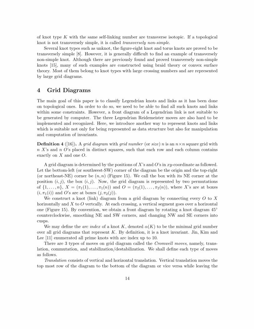
Definition 4 ([16]). A grid diagram with grid number (or size) 𝑛 is an 𝑛×𝑛 square grid with𝑛 𝑋’s and 𝑛 𝑂’s placed in distinct squares, such that each row and each column containsexactly on 𝑋 and one 𝑂.

A grid diagram is determined by the positions of𝑋’s and𝑂’s in 𝑥𝑦-coordinate as followed.Let the bottom-left (or southwest-SW) corner of the diagram be the origin and the top-right(or northeast-NE) corner be (𝑛, 𝑛) (Figure 15). We call the box with its NE corner at theposition (𝑖, 𝑗), the box (𝑖, 𝑗). Now, the grid diagram is represented by two permutationsof {1, . . . , 𝑛}, 𝑋 = (𝜋1(1), . . . , 𝜋1(𝑛)) and 𝑂 = (𝜋2(1), . . . , 𝜋2(𝑛)), where 𝑋’s are at boxes(𝑖, 𝜋1(𝑖)) and 𝑂’s are at boxes (𝑗, 𝜋2(𝑗)).

We construct a knot (link) diagram from a grid diagram by connecting every 𝑂 to 𝑋horizontally and 𝑋 to 𝑂 vertcally. At each crossing, a vertical segment goes over a horizontalone (Figure 15). By convention, we obtain a front diagram by rotating a knot diagram 45∘

counterclockwise, smoothing NE and SW corners, and changing NW and SE corners intocusps.

We may define the arc index of a knot 𝐾, denoted 𝛼(𝐾) to be the minimal grid numberover all grid diagrams that represent 𝐾. By definition, it is a knot invariant. Jin, Kim andLee [11] enumerated all prime knots with arc index up to 10.

There are 3 types of moves on grid diagram called the Cromwell moves, namely, trans-lation, commutation, and stabilization/destabilization. We shall define each type of movesas follows.Translation consists of vertical and horizontal translation. Vertical translation moves the

top most row of the diagram to the bottom of the diagram or vice versa while leaving the

14

X

O

X

O

X

O

X

O

(a) unknot

X

O

X

O

X

O

X

O

X

O

(b) trefoil

Figure 15: Grid Diagrams and Corresponding Knot Diagrams

rest unchanged. Horizontal translation, similarly, moves the leftmost column of the diagramto the rightmost or vice versa. We can consider a class of grid diagrams modulo translationas a diagram drawn on a torus.Commutation interchanges two adjacent rows or two adjacent columns satisfying the

following conditions.

1. To commute two rows (or columns), four 𝑋’s and 𝑂’s in those rows (or columns) mustlie in different columns (or rows).

2. Line segments connecting 𝑋’s and 𝑂’s in the rows (or columns) must be either nested,or disjoint (see Figure 16).

Lastly, destabilization replaces a 2×2 subgrid containing two 𝑋’s and one 𝑂’s (or two𝑋’sand one 𝑂’s) by a 1× 1 subgrid containing 𝑂 (or 𝑋), and results in a grid diagram with onefewer row and one fewer column as in Figure 17. Stabilization is simply an inverse processof destabilization. Hence, there are 8 types of (de)stabilization, denoted by 𝑋:NW, 𝑋:NE,𝑋:SW, 𝑋:SE, 𝑂:NW, 𝑂:NE, 𝑂:SW, and 𝑂:SE. The first part corresponds to the letter ina 1× 1 subgrid, and the second part corresponds to the position of the empty box in 2× 2subgrid. Note that one can write any 𝑂 (de)stabilization by a composition of translations,commutations and exactly one 𝑋 (de)stabilization of the diagonally opposite position (e.g.NE is diagonally opposite to SW). Thus, we may consider only 𝑋 (de)stabilization as a typeof Cromwell moves.

15

X

O

X

O

X

O

X

O

X

O

X

O

X

O

X

O

X

O

(a) nested

X

O

X

O

X

O

X

O

X

O

X

O

X

O

X

O

X

O

(b) disjoint

Figure 16: Commutation

X

O

X

O

X

O

X

O

X

O

X

O

X

O

X

O

↔X

O

X

O

X

O

X

O

X

O

X

O

X

O

Figure 17: Destabilization

Let 𝒢 denote the set of all grid diagrams, ℒ the set of all oriented Legendrian links upto Legendrian isotopy, 𝒯 the set of all oriented transverse links up to transveral isotopy, 𝒦the set of all oriented links up to topological isotopy, and let 𝒢 denote the quotient of 𝒢 bytranslation and commutation. Ng and Thurston have shown in [16] that there are bijections

𝒢/(𝑋 : 𝑁𝐸,𝑋 : 𝑆𝑊 ) → ℒ𝒢/(𝑋 : 𝑁𝐸,𝑋 : 𝑆𝑊,𝑋 : 𝑆𝐸) → 𝒯

𝒢/(𝑋 : 𝑁𝐸,𝑋 : 𝑆𝑊,𝑋 : 𝑆𝐸,𝑋 : 𝑁𝑊 ) → 𝒦

induced by the above construction of a front diagram from a grid diagram.Besides three types of Cromwell moves, we shall define a few other significant operations

on grid diagrams. We define the symmetry of grid diagram which reflects the diagram aboutthe NW-SE diagonal and interchanges 𝑋’s and 𝑂’s to be 𝑆2. Ng and Thurston [16] showthat 𝑆2 operation on a grid diagram preserves Legendrian isotopy.

Given a Legendrian link 𝐿, we may define a Legendrian mirror of 𝐿, denoted 𝜇(𝐿), to

16

be a Legendrian link represented by the front diagram which is the reflection of the frontdiagram of 𝐿 in horizontal axis. This operation preserves topological type but generally donot preserve Legendrian isotopy. Let −𝐿 be a Legendrian link which has the same frontdiagram as 𝐿 but with orientation reverse. These two operations can easily be defined on griddiagram by rotating the grid diagram by 180∘ and interchanging 𝑋’s and 𝑂’s, respectively.

X

O

X

O

X

O

X

O

X

O

X

O

(a) original diagram

X

O

X

O

X

O

X

O

X

O

X

O

(b) 𝑆2

X

O

X

O

X

O

X

O

X

O

X

O

(c) Legendrian mirror

X

O

X

O

X

O

X

O

X

O

X

O

(d) orientation reversal

Figure 18: Operation on grid diagrams

In the case of representing unoriented links by grid diagrams, 𝑋 and 𝑂 are interchange-able. Hence we may replace all 𝑋’s and 𝑂’s by the same symbol, says ‘1’. We replace allempty grids by ‘0’ and obtain a matrix with only 0’s and 1’s, called Cromwell matrix. ACromwell matrix has exactly two 1’s in each row and each column. Consisting of binarynumbers, a Cromwell matrix is the most convenient form of a link to be implemented inprogramming. Similarly, we can construct a knot (link) diagram of an unoriented knot (link)from a Cromwell matrix by connecting 1’s in the same row or the same column such thata vertical segment goes over a horizontal one. We can also turn the diagram 45∘ counter-clockwise to get an unoriented Legendrian front diagram.

We may define translation, commutation, and (de)stabilization on Cromwell matricesanalogous to those on grid diagrams but ignoring the difference between 𝑋 and 𝑂. We saytwo Cromwell matrices are equivalent if they relate by a sequence of translations, commu-tations and 𝑋 : 𝑁𝐸, 𝑋 : 𝑆𝑊 (de)stabilizations. This definition is well-defined even thoughwe do not distinguish 𝑋 and 𝑂 because 𝑂 : 𝑁𝐸 and 𝑂 : 𝑆𝑊 can be written as 𝑋 : 𝑆𝑊 and𝑋 : 𝑁𝐸, respectively. In other word, two Cromwell matrices are equivalent if they represent

17

two unoriented Legendrian isotopic links.Note that a stabilization increases the size of a Cromwell matrix by one. Thus, for any

Cromwell matrix of size 𝑛, there are equivalent Cromwell matrices of size 𝑛 + 1, 𝑛 + 2, . . ..Since we will generate links by their size and we only distinguish them up to Legendrianisotopy, links of the same type will show up again while we generate matrices of larger sizes.To prevent this reoccurence of links of the same type, we introduce a notion of irreducibility,which will reduce redundancy in our algorithm.

Definition 5 ([11]). A Cromwell matrix is reducible if two 1’s in a row or a column areadjacent up to a cyclic permutation of entries.

If a Cromwell matrix is not reducible, we say it is irreducible. It is easy to implementan algorithm to check whether a given Cromwell matrix is reducible. A reducible Cromwellmatrix represents a grid diagram which can be destabilized. Hence, an 𝑛 × 𝑛 reducibleCromwell matrix does not represent a topological link with arc index 𝑛. In other words, if aCromwell matrix of size 𝑛 represents a topological link with arc index 𝑛, then any Cromwellmatrix in the same equivalence class has size at least 𝑛. In particular, any Cromwell matrixobtained from such matrix by a sequence of translations and commutations is irreducible.However, it is not necessarily true that if every matrix obtained from a Cromwell matrixof size 𝑛 by a sequence of translations and commutations is irreducible, then the Cromwellmatrix represents a topological link with arc index 𝑛.

5 Algorithms

Our classification of Legendrian knots and links will be done for each grid number at a time.From the previous section, there is a 2𝑛-to-one correspondence between grid diagrams andCromwell matrices, where 𝑛 is the number of components (𝑛 = 1 for knots). Furthermore,the correspondence preserves equivalence class under translation, commutation and 𝑋:NE,𝑋:SW (de)stabilization. Thus, we can obtain all irreducible grid diagrams by generatingall irreducible Cromwell matrices. Although the uniqueness up to Lengendrian isotopy maynot be preserved, comparing as Cromwell matrices greatly reduces work to be done to griddiagrams as there are fewer Cromwell matrices and fewer possible moves.

For each grid number 𝑛, the classification is done in three main steps.

1. Generating all Cromwell matrices, unique up to translation and commutation

2. Reducing Cromwell matrices to be unique up to unoriented Lengendrian isotopy

3. Reducing grid diagrams to be unique up to oriented Lengendrian isotopy

18

5.1 Generating all Cromwell matrices, unique up to translation and com-mutation

We modify the algorithm used to classify topological knots by Jin, Kim and Lee in [11].First, we introduce a way to order Cromwell matrices by assigning a distinct integer to eachCromwell matrix.

Definition 6 ([11]). The norm of an 𝑛 × 𝑛 Cromwell matrix is the natural number corre-sponding to the binary number obtained by concatenating its rows.

For example, the norm of ⎡⎢⎢⎢⎢⎣

1 0 0 1 00 1 0 0 11 0 1 0 00 1 0 1 00 0 1 0 1

⎤⎥⎥⎥⎥⎦

is 10010010011010001010001012 .This definition of norm allows us to generate Cromwell matrices in norm-decreasing

order. Beginning with an ’empty’ matrix with 0 in every entry, we can create a Cromwellmatrix by replacing 2𝑛 0’s with 1’s, one at a time. We start from the left 1 in the top row,the right 1, then the left 1 in the second row, and so on. We can reduce number of possiblechoices of placing 1’s by taking translation, commutation and reducibility into account.

As our goal is to generate irreducible Cromwell matrices, we shall not place two 1’s next toeach other vertically or horizontally. Moreover, we can eliminate the choice of placing in sucha way that we can easily get a reducible matrix by translations or commutations. In addition,we can also omit the choice that norm may increase by translations or commutations. Thus,we require that all Cromwell matrices we generate must have a 1 at the leftmost column ofthe first row. We shall use tree structure to represent each step of placing 1 to an emptymatrix (Figure 19). We let the matrix with only one 1 be the root of the tree (depth 0).By the previous constraint, there are ⌈𝑛−3

2 ⌉ possible positions to place the second 1 withoutmaking the matrix reducible and also avoiding redundancy. Hence, there are ⌈𝑛−3

2 ⌉ nodesin the next level (depth 1) of the tree. The third 1 cannot be placed right below any of theprevious ones. The fourth 1 must be as far from the third as the distance between the firsttwo 1’s. Otherwise, we can translate them to the first row and get larger norm. By takingthese conditions into account, we similarly generate nodes in the fifth, the sixth, and so on,until we reach the last level (depth 2𝑛− 1). Only the nodes in the last level are complete asCromwell matrices.

For each Cromwell matrix generated in this way, we check and eliminate the matrix if ithas one of the following properties:

1. the matrix represents link with incorrect number of components (more than 1 if weonly consider knots)

19

Figure 19: Tree structure for generating Cromwell matrices of size 5

2. translations and/or commutations increase its norm

3. it becomes reducible after a sequences of translations and/or commutations

Cromwell matrices left from this algorithm with be unique up to translations and com-mutations, and have the highest norm among those in the same equivalence class.

5.2 Reducing Cromwell matrices to be unique up to unoriented Lengen-drian isotopy

Now we are ready to classify unoriented Legendrian links generated in the previous step.Recall that any two Legendrian links are equivalent if and only if they relate by translations,commutations and 𝑋:NE, 𝑋:SW (de)stabilizations. We simply have an algorithm to deter-mine whether two Cromwell matrices represent the same Legendrian links by repeatedlyapply the corresponding moves to one matrix until it to become another one. However, thisalgorithm is indeterministic. That is, if the two matrices represent inequivalent Legendrian

20

links, the algorithm does not halt and goes on forever. Even though the two matrices repre-sent the same Legendrian link, we do not know how many moves it may take to transformone to the other. Although there is no simple known deterministic algorithm to determinewhether two Legendrian links are equivalent, we can improve this simple algorithm to aidus in making conjectures in the classification.

We can consider this problem as a path searching problem on a graph: let each griddiagram (or Cromwell matrix) be represented by a vertex, and two vertices are connected ifthey represent grid diagrams that relate by one step of those moves. Since each Cromwellmove is reversible, the graph is thus undirected. Hence, the algorithm to determine whethertwo grid diagrams represent the same Legendrian links is equivalent to the algorithm todetermine whether there is a path connecting two vertices on a given graph (with infinitenumber of vertices). Hence, we may apply any path searching algorithm to answer thisquestion.

Generally, a simple path searching algorithm will start at an initial vertex and searchalong each edge connected from the initial vertex until reaching the goal. Theoretically, thisalgorithm should be able to determine whether there exists a path connecting the given twovertices. However,

1. a graph representing all possible grid diagrams is infinitely large as we can alwaysstabilize a grid diagram to get a larger one

2. the graph is not given but need to be generated while searching

3. degree at each vertex is very high.

Since we have limited computing resource, we have to optimize our algorithm in everypossible way.

Instead of regular search algorithm, we use bidirectional search algorithm to determinewhether there exists a path connecting two vertices. This algorithm is appropriate in ourcircumstance because the moves are reversible and similar in both directions, and goal stateis clear. Note again that this algorithm is undecidable. In the case that two diagrams arenot related by any number of moves, i.e. they represent different Legendrian links, thisalgorithm does not halt. Hence, we need to specify number of steps it will compute. As aresult, this algorithm may take very long time to check all possible pairs of grids we havegenerated if we allow a large number of step.

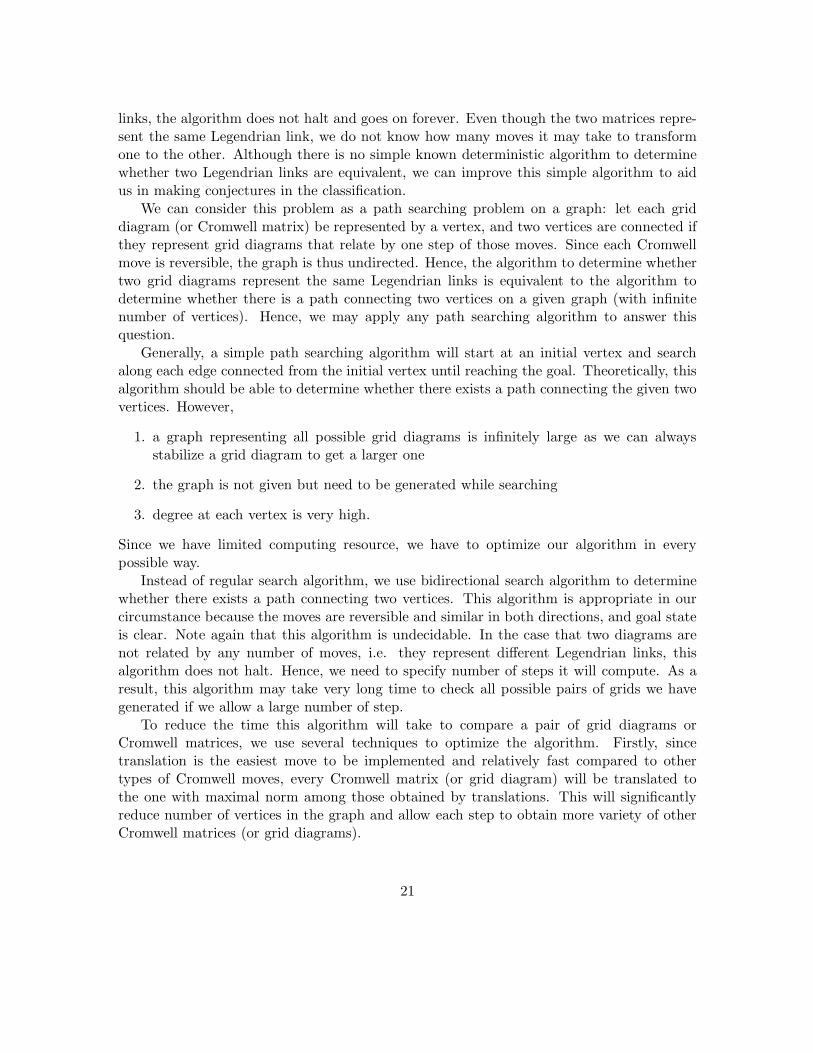
To reduce the time this algorithm will take to compare a pair of grid diagrams orCromwell matrices, we use several techniques to optimize the algorithm. Firstly, sincetranslation is the easiest move to be implemented and relatively fast compared to othertypes of Cromwell moves, every Cromwell matrix (or grid diagram) will be translated tothe one with maximal norm among those obtained by translations. This will significantlyreduce number of vertices in the graph and allow each step to obtain more variety of otherCromwell matrices (or grid diagrams).

21

We can also reduce number of steps the algorithm would take to get from one Cromwellmatrix (or grid diagram) to another by allowing non-Cromwell moves that preserve Legen-drian isotopy. By doing so, although each vertex will have higher degree, number of edgesin the graph will be reduced significantly. Thus, for each vertex representing a Cromwellmatrix (or grid diagram) 𝐷, we generate adjacant vertices as follows:

1. all Cromwell matrices (or grid diagrams) generated by applying one commutation to𝐷, do not exist if 𝐷 does not contain nested or disjoint rows or columns

2. all Cromwell matrices (or grid diagrams) generated by applying one 𝑋:NE, 𝑋:SWstabilization at the top left box in 𝐷, which we assume to be 1 (for Cromwell matrix)(or 𝑂 for grid diagram, in which case we will use 𝑂:NE and 𝑂:SW)

3. all Cromwell matrices (or grid diagrams) generated by applying one 𝑋:NE, 𝑋:SWdestabilization to 𝐷, do not exist if 𝐷 is not reducible

4. a Cromwell matrix (or grid diagram) generated by applying 𝑆2 to 𝐷

5. all Cromwell matrices (or grid diagrams) generated by applying the speed up move to𝐷, may not exist if 𝐷 does not contain the specific pattern

where the speed up move is defined locally as in Figure 20 together with its rotation reverseand 180∘ rotation. Note that this constitutes a Legendrian isotopy since it only involves𝑋:NE and 𝑋:SW (equivalently, 𝑂:SW and 𝑂:NE) (de)stabilization.

Figure 20: Speed up move

We call any one of the above a step. Note that we only apply a stabilization to one boxin 𝐷 since we can move it to any other places using commutations. We choose the top leftbox because it will always be 1 for Cromwell matrix or 𝑂 for grid diagram if 𝐷 has maximalnorm up to translation.

22

Let IsLegendrianIsotopic(𝑑, 𝑠) be the algorithm to check whether two Cromwell matri-ces (or grid diagrams) represent the same Legendrian link while allowing no more than 𝑑 stepsand the grid size is never more than 𝑠. We can describe IsLegendrianIsotopic(𝑑, 𝑠)(𝐷1,𝐷2)as follows:

1. begin with two sets of Cromwell matrices (or grid diagrams), 𝐴 = {𝐷1} and 𝐵 = {𝐷2};also let 𝐴′ = ∅ and 𝐵′ = ∅

2. for each 𝐷 ∈ 𝐴,∙ move 𝐷 to 𝐴′

∙ for each 𝐷′, a Cromwell matrix (or grid diagram) generated from 𝐷 in one step,put 𝐷′ in 𝐴 if 𝐷′ is not in 𝐴′ and size of 𝐷′ is at most 𝑠

3. check whether 𝐴 ∩𝐵 = ∅; if not, halt and return true

4. repeat the two previous steps with 𝐴 and 𝐵 switched

5. repeat the last three steps 𝑑 times or until this algorithm halts.

Since there are finitely many grid diagrams of size at most 𝑠, IsLegendrianIsotopic(𝑑, 𝑠)must halt for any 𝑑 ∈ ℕ ∪ {∞}.

If 𝐷1,𝐷2 are grid diagrams, by allowing 𝑋 : 𝑆𝐸 (de)stabilization, this algorithm canbe applied to the problem of determining whether they represent the same transverse link.Similarly, by allowing both 𝑋:SE and 𝑋:NW (de)stabilization, this algorithm can also beapplied to the problem of determining whether two Cromwell matrices (or grid diagrams)represent the same topological link.

In order to reduce the number of comparison, we can use other methods to eliminatepairs of diagrams which do not represent the same Legendrian knots. These methods mustbe a lot faster than directly comparing. Classical invariants such as rotation number (𝑟) andThurston-Bennequin number (𝑡𝑏) are easy to compute and effective in decreasing number ofpairs the actual comparison required since we do not need to check pairs with different 𝑟 or𝑡𝑏. We only use these two invariant for arc index up to 8. For arc index 9, we also checkfor topological knot type of each grid diagrams as another invariant since several knot typeshave the same 𝑡𝑏.

Instead of comparing two diagrams at a time, we can also improve our bidirectionalsearch algorithm to check for any number of grid diagrams by beginning with each setcontaining each diagram we consider and comparing them all at once. For larger arc index,there are many grid diagrams which classical invariants cannot classify. As it takes longer togenerate new grid diagrams, comparing many grid diagrams at once can make the processsignificantly faster.

23

5.3 Reducing grid diagrams to be unique up to oriented Lengendrianisotopy

The previous step gives us a set of Cromwell matrices that potentially represent distinctunoriented Legendrian knots. However, our goal is to classify oriented Legendrian knots.We then need to assign orientations to each unoriented Legendrian knots represented byCromwell matrices. For a knot, which is a one-component link, this step is simply to assignthe 1 at the left upper corner to be either 𝑂 or𝑋 as the rest will be completely determined bythe first one. Generally, for a link with 𝑛 components, we get 2𝑛 oriented links by assigning𝑂 or 𝑋 to one box for each of the 𝑛 components. These generated grid diagrams may relateby a sequence of Cromwell moves and thus represent knots that are Legendrian isotopic.

We can repeat the above algorithm on grid diagrams representing Legendrian knots thatwe cannot simply distinguish by classical invariants. The reason that we apply this algorithmboth before and after assigning orientation is to reduce number of comparison that need tobe made. Note that if two unoriented Legendrian knots cannot be shown to be the same bythe algorithm IsLegendrianIsotopic(∞, 𝑠), they still cannot be shown to be the same afterbeing assigned orientations. However, this may not be true for IsLegendrianIsotopic(𝑑, 𝑠)for some finite 𝑑 because the top left corner of an oriented diagram is always set to be 𝑂and the stabilization takes place at that box for knot case. Thus, if the top left corner of anunoriented diagram (a Cromwell matrix) is assgined to be 𝑋 when given orientation, it willget translated so that the box at top left corner becomes 𝑂 and therefore alter the positionwhere stabilization will occur.

6 Distinguish Legendrian Knots

Remind that our algorithm cannot show that two Legendrian knots are not Legendrianisotopic. The three classical Legendrian invariants alone are not enough to classify Legen-drian knots, even for small ones such as type 𝑚(52). In this section, we will use severalnon-classical invariants to distinguish Legendrian knots which share topological type, 𝑡𝑏 and𝑟.

We use the Mathematica notebook Legendrian invariants.nb from [18] to computepolynomials for graded ruling invariant and linearized contact homology. In Legendrian

invariant.nb, the graded ruling invariant of a Legendrian knot 𝐿 is written as a polynomial∑𝑖 𝑎𝑖𝑧

𝑖 where 𝑎𝑖 is the number of graded rulings 𝑅 with 𝛾(𝑅) = 𝑖. Note that these twoLegendrian invariants are defined only on Legendrian knots with 𝑟 = 0. Thus, they cannotbe used to distinguish several pairs of Legendrian knots such as two knots of type 63. Theyare also invariant under orientation reversal and Legendrian mirror, and hence cannot beused to distinguish pairs of Legendrian knots that are orientation reversal and Legendrianmirror of each other.

Despite such limitation, graded ruling invariant and linearized contact homology arevery useful and can be used to classify several pairs of Legendrian knots. The Legendrian

24

knots that can be distinguished using graded ruling invariant are those of type𝑚(52), 𝑚(72),73, 74, 𝑚(75), 𝑚(76), 𝑚(945), 948, 949, 10128, 10136, 10142 and 10160. By using linearizedcontact homology, we can further distinguish pairs of type 𝑚(61) and 𝑚(72) that cannot bedone using graded ruling invariant though they can be distinguished using 𝜌-graded rulinginvariants for some integer 𝜌.

We can see from table 1 that we can use linearized contact homology to distinguish everypair that we can do by graded ruling invariant. However, it is still useful to mention gradedruling invariant as it is easier to compute by hand, and it is not true in general that any pairof knot distinguished by graded ruling invariant can be distinguished by linearized contacthomology.

Furthermore, Ng [13] provides a technique using the Chekanov-Eliashberg differentialgraded algebra (DGA) which can be used to distinguish between several pairs that cannotbe distinguished by any invariants mentioned earlier. In his paper, Ng distinguishes

1. two Legendrian knots of type 62 with (𝑡𝑏, 𝑟) = (−7, 0) which correspond to the firstgrid diagram of type 62 in the table and its Legendrian mirror

2. two Legendrian knots of type 63 with (𝑡𝑏, 𝑟) = (−4, 1) which correspond to two griddiagrams of type 63 in the table

3. two Legendrian knots of type𝑚(72) with (𝑡𝑏, 𝑟) = (1, 0) which correspond to the secondand the fourth grid diagrams of type 𝑚(72) in the table

4. two Legendrian knots of type 74 with (𝑡𝑏, 𝑟) = (1, 0) which correspond to the secondand the third grid diagrams of type 74 in the table.

The Chekanov-Eliashberg DGA can also be used to distinguish the first and the third griddiagrams of type 74, and the third grid diagrams of the same type with its Legendrianmirror.

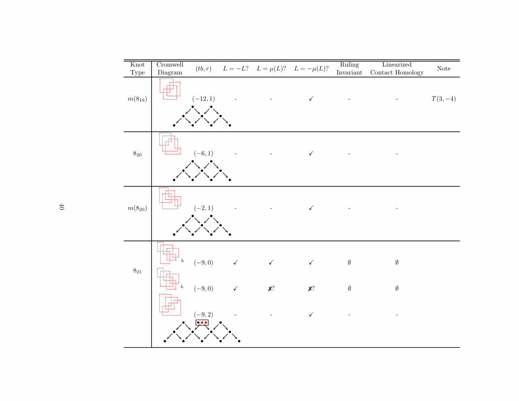
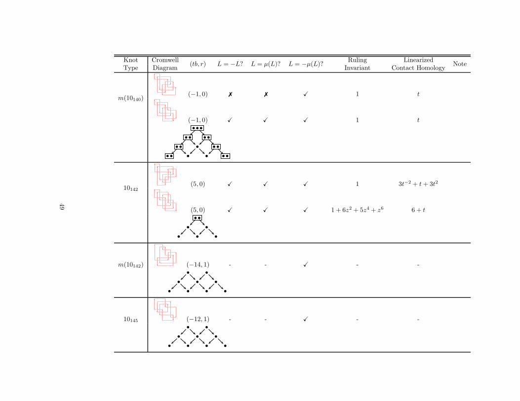
As we mentioned earlier, we can view Legendrian knot as a subtype of transverse knot.In other words, if two knots are not transverse isotopic, they are not Legendrian isotopic.Ng, Ozsvath and Thurston [15] provide a technique using knot Floer homology, based onthe work of Ozsvath, Szabo and Thurston [17], to distinguish several pairs of transverseknots. We can apply the same technique to distinguish some pairs of Legendrian knots inthe table. In [15], two transverse knots, corresponding to the first grid diagram and itsLegendrian mirror of type 𝑚(10132) are distinguished. Since the second grid diagram istransversal isotopic to the first grid and Legendrian isotopic to its own mirror, it cannotbe Legendrian isotopic to the first grid. Hence, we can conclude that 3 grid diagrams withknot type 𝑚(10132) represent 3 distinct Legendrian knots. In the same manner, we candistinguish three Legendrian knots with (𝑡𝑏, 𝑟) = (−1, 0) of type 𝑚(10140). Moreover, wecan identify transversely non-simple knots of type 𝑚(10145), 𝑚(10161) and 12𝑛591, each ofwhich lies in the second level (from above) in the mountain range of its type.

25

7 Legendrian Knot Atlas

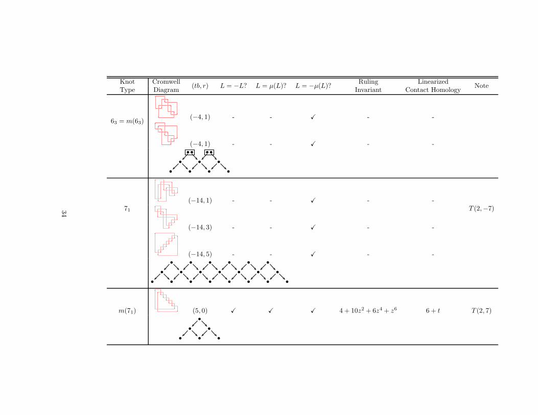
The result of our algorithm together with invariants and techniques described in previoussection gives the Legendrian knot atlas as shown in table 1. From our generated griddiagrams, we use gridlink [5] to draw diagrams, each of which can be rotated 45∘ to get a frontdiagram. Note that we do not show all grid diagrams of each knot type. However, readers canfind all grid diagrams from the table by using Legendrian mirror and/or orientation reversalas described earlier. Note again that these two operations preserve graded ruling invariantand linearized contact homology which also depicted in the table. Since orientation reversalwill negate 𝑟, we only illustrate Legendrian knots with nonnegative 𝑟. Again, readers canfind grid diagrams for negative 𝑟 by reversing orientation. We also provide the mountainrange of each knot type in the table, some of which have been proven while the rest areconjecture drawn from the result of our algorithm and the previous section.

For columns labeled 𝐿 = −𝐿?, 𝐿 = 𝜇(𝐿)? and 𝐿 = −𝜇(𝐿)?, we use ✓ to indecate pairsof grid diagrams which our algorithm can show that they represent the same Legendrianknot. For example, the 𝑡𝑏 = 1, 𝑟 = 0 Legendrian knot 𝐿 of type 𝑚(31) is Legendrianisotopic to its orientation reversal (−𝐿), its Legendrian mirror (𝜇(𝐿)) and the orientationreversal of its Legendrian mirror (−𝜇(𝐿)). We use ✗ to indicate pairs of grid diagramswhich can be distinguished by some invariants and/or techniques described above. We use✗? to indicate pairs of grid diagrams which our algorithm cannot show that they representthe same Legendrian knot, but cannot be distinguished by any invariants or techniquesdescribed above. The letters subscripted under some pairs of grid diagrams also indicatesets of Legendrian knots that cannot be distinguished by those invariants and techniques.

Since orientation reversal and Legendrian mirror negate rotation number, for grid dia-grams with 𝑟 ∕= 0, orientation reversal and Legendrian mirror cannot be Legendrian isotopicto the original. We use − to indicate such case. Similarly, since graded ruling invariant andlinearized contact homology are not defined on grid diagrams with 𝑟 ∕= 0, such boxes areindicated by −. Note that − is different from ∅ which is when 𝑟 = 0 but there are no gradedrulings or linearized contact homology.

In moutain range, we use a box containing more than one dot to indicate that there are(conjecturally if other dots are red) more than one Legendrian knot with the same 𝑡𝑏 and 𝑟.Number of black dots in the box corresponds to number of grid diagrams that can be provedto represent distinct Legendrian knots with that particular 𝑡𝑏 and 𝑟. Number of black andred dots together corresponds to number o grid diagrams that our algorithm cannot showthat any pairs of them represent the same Legendrian knots. We also omitted axes of 𝑡𝑏 and𝑟 as they can be inferred from 𝑡𝑏 and 𝑟 of the grid diagrams.

Our result agrees with mountain ranges of torus knots and the figure eight knot describedby Etnyre and Honda in [8], and also agrees with mountain ranges of twist knots describedby Etnyre, Ng and Vertesi in [9]. We indicate torus knots by 𝑇 (𝑝, 𝑞) and twist knots by𝐾𝑚 (notation as in [9]) in “Note” column. Moreover, the result gives more conjectures formountain ranges of all prime knots with arc index up to 9. Since we generated grid diagrams

26

up to size 10, all grid diagrams of size at most 10 of each knot type are shown in its mountainrange. The black dots in the mountain range are the lower bound on what mountain rangeof each knot type is, i.e., the smallest possible mountain range. However, we conjecturethe mountain ranges to consist of both black dots and red dots. It is still possible that themountain ranges of some knot types are larger than we describe, but any Legendrian knotsnot shown in the mountain range, if exist, must be represented by grid diagrams of size 11or higher.

The mountain range of each knot type also gives an information on transverse knots.We see from the previous section that classes of transverse knots are equivalent to classes ofLegendrian knots modulo negative stabilization. Hence, we can read of classes of transverseknots of each knot type from its mountain range and relations of Legendrian classes undernegative stabilization. This results in a transverse knot atlas as shown in table 2. We usesimilar notations as in the Legendrian knot atlas described above. Knot types that areshown to be transversely nonsimple are labeled in blue and knot types that we conjectureto be transversely nonsimple but cannot prove are labeled in red.

8 Legendrian Links

In the previous section, we focused the classification entirely on Legendrian knots and weleft out all grid diagrams that represent links with more than one component in generatingstep of our algorithm. Note that, with little modification, the following step of the algorithmalso works for links with more than one component. The main differences for links with 𝑛components are as follows:

1. there are 2𝑛 different possible orientations for each unoriented link (Cromwell diagram)although some of them may be Legendrian isotopic

2. there are 𝑛 positions for stabilization, one in each component

3. may need to keep track of two distinct components in the case that they cannot beswitched topologically

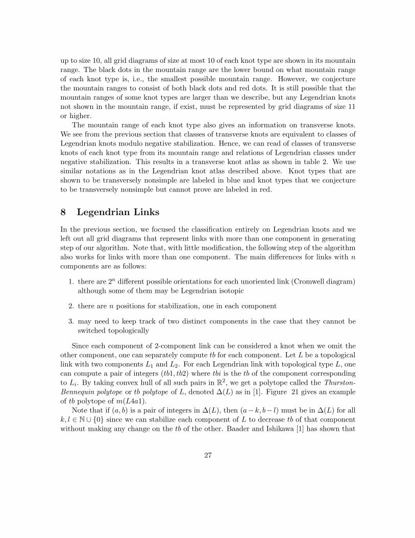
Since each component of 2-component link can be considered a knot when we omit theother component, one can separately compute 𝑡𝑏 for each component. Let 𝐿 be a topologicallink with two components 𝐿1 and 𝐿2. For each Legendrian link with topological type 𝐿, onecan compute a pair of integers (𝑡𝑏1, 𝑡𝑏2) where 𝑡𝑏𝑖 is the 𝑡𝑏 of the component correspondingto 𝐿𝑖. By taking convex hull of all such pairs in ℝ

2, we get a polytope called the Thurston-Bennequin polytope or 𝑡𝑏 polytope of 𝐿, denoted Δ(𝐿) as in [1]. Figure 21 gives an exampleof 𝑡𝑏 polytope of 𝑚(𝐿4𝑎1).

Note that if (𝑎, 𝑏) is a pair of integers in Δ(𝐿), then (𝑎− 𝑘, 𝑏− 𝑙) must be in Δ(𝐿) for all𝑘, 𝑙 ∈ ℕ ∪ {0} since we can stabilize each component of 𝐿 to decrease 𝑡𝑏 of that componentwithout making any change on the 𝑡𝑏 of the other. Baader and Ishikawa [1] has shown that

27

-4 -3 -2 -1 0

-4

-3

-2

-1

0

�

�

�

Figure 21: Thurston-Bennequin polytope of 𝑚(𝐿4𝑎1)

for two-bridge link 𝐿 with two components 𝐿1 and 𝐿2

Δ(𝐿) = {(𝑥1, 𝑥2) ∈ ℝ∣𝑥1 ≤ −1, 𝑥2 ≤ −1, 𝑥1 + 𝑥2 ≤ 𝑡𝑏(𝐿)− 2𝑙𝑘(𝐿1, 𝐿2)}.

However, the 𝑡𝑏 polytope is not known in general case.Let ℒ = ℒ1 ∪ ℒ2 be a Legendrian link with two components ℒ1 and ℒ2. Let 𝐿 be

a topological link type of ℒ with components 𝐿1 and 𝐿2 corresponding to ℒ1 and ℒ2,respectively. Then it follows from the definition that

𝑡𝑏(ℒ) = 𝑡𝑏(ℒ1) + 𝑡𝑏(ℒ2) + 2𝑙𝑘(𝐿1, 𝐿2).

Similarly, we may calculate

𝑡𝑏(ℒ1 ∪𝐷(ℒ2)) = 𝑡𝑏(ℒ1) + 4𝑡𝑏(ℒ2) + 4𝑙𝑘(𝐿1, 𝐿2)

from the construction of double of 𝐿 in previous section. For each value of 𝑡𝑏(ℒ2), we canfind a good bound for 𝑡𝑏(ℒ1) by using Theorem 3.2 on 𝐿1 ∪𝐷𝑡𝑏(ℒ2)(𝐿2). This is similar tothe technique used in [14]. We have

𝑡𝑏(ℒ1) ≤ 𝑡𝑏(𝐿1 ∪𝐷𝑡𝑏(ℒ2)(𝐿2))− 4𝑡𝑏(ℒ2)− 4𝑙𝑘(𝐿1, 𝐿2).

We may repeat this calculation but double ℒ1 instead of ℒ2. The bound on both partscan be used to give an upper bound on Δ(𝐿). However, the calculation of the Khovanovpolynomial for very large links in KnotTheory` package sometimes fails due to running timeor memory limitation.

Using our algorithm and invariants in previous sections, we get an atlas for unorientedLegendrian two-component links as shown in table 3. The atlas shows the representation ofgrid diagrams which can be turned 45∘ to get unoriented front diagrams. In the case whentwo components cannot be switched topologically, we also distinguish them by color andsize of strands. We also provide our conjecture for 𝑡𝑏 polytope of each link type. Note that

28

our result can answer the question posted by Baader and Ishikawa in [1] that whether the𝑡𝑏 polytope can always be described by three linear inequalities of the type

𝑡𝑏(ℒ1) ≤ 𝑛1, 𝑡𝑏(ℒ2) ≤ 𝑛2, 𝑡𝑏(ℒ1) + 𝑡𝑏(ℒ2) ≤ 𝑛3.

Counterexamples illustrated on table 3 are links that cannot be described by three linearinequalities, 𝑚(𝐿7𝑎1), 𝐿9𝑛18, 𝑚(𝐿10𝑛54) and 𝐿11𝑛204, and links that can be described bythree linear inequalities but not of the above type, 𝐿9𝑛19, 𝐿10𝑛24 and 𝑚(𝐿11𝑛205).

Acknowledgements

First and foremost, I offer my sincerest gratitude to my mentor, Lenhard Ng, for suggest-ing this project, guiding me during the summer and my senior year, and supporting methroughout my thesis. I am thankful to Daniel Rutherford for reading the paper and givingvaluable comments. I am grateful to all faculties and staff at Duke University MathematicsDepartment, especially David Kraines, for the support during my undergraduate career.Lastly, I would like to thank my family and friends for supported me in any aspect duringthe completion of the project.

References

[1] S. Baader and M. Ishikawa, Legendrian framings for two-bridge links; arXiv:

0910.0355v1 [math.GT].

[2] D. Bar-Natan, The Mathematica Package KnotTheory`, available from http://

katlas.math.toronto.edu/wiki/The Mathematica Package KnotTheory`.

[3] D. Bennequin, Entrelacements et equations de Pfaff, Asterisque 107-108 (1983), 87-161.

[4] Y. V. Chekanov and P. E. Pushkar, Combinatorics of fronts of Legendrian links, andArnold’s 4-conjectures, Uspekhi Mat. Nauk 60 (2005), no. 1 (361), 99-154.

[5] M. Culler, Gridlink, available from http://www.math.uic.edu/˜culler/gridlink/.

[6] J. Epstein, D. Fuchs and M. Meyer, Chekanov-Eliashberg invariants and transverseapproximations of Legendrian knots, Pacific Journal of Mathematics 201 (2001), no.1, 89-106.

[7] J. B. Etnyre, Legendrian and transversal knots, in The Handbook of knot theory, 105-185, Elsevier B.V., Amsterdam, 2005.

[8] J. B. Etnyre and K. Honda, Knots and contact geometry I: Torus knots and the figureeight knot, J. Symplectic Geom. 1 (2001), no. 1, 63-120.

29

[9] J. B. Etnyre, L. Ng and V. Vertesi, Legendrian and transverse twist knots; arXiv:

1002.2400v1 [math.SG].

[10] D. Fuchs and S. Tabachnikov, Invariants of Legendrian and transverse knots in thestandard contact space, Topology 36 (2007), no. 5, 1025-1053.

[11] G. T. Jin, H. Kim and G. Lee, Prime knots with arc index up to 10, in Intelligence ofLow Dimensional Topology 2006, 65-74, Eds. J. Scott Carter et al, 2007.

[12] L. Ng, A Legendrian Thurston-Bennequin bound from Khovanov homology, Algebr.Geom. Topo. 5 (2005), 1637-1653; math/0508649.

[13] L. Ng, Computable Legendrian Invariants, Topology 42 (2003), no. 1, 55-82; arXiv:math.GT/0011265.

[14] L. Ng, On arc index and maximal Thurston-Bennequin number; math.GT/0612356v3

[15] L. Ng, P. Ozsvath and D. Thurston, Transverse knots distinguished by knot Floerhomology, Journal of Symplectic Geometry 6 (2008), no. 4, 461-490.

[16] L. Ng and D. Thurston, Grid diagrams, braids, and contact geometry, in Proceedingsof 15𝑡ℎ Gokova Geometry-Topology Conference, 120-136; arXiv:0812.3665.

[17] P. Ozsvath, Z. Szabo and D. Thurston, Legendrian knots, transverse knots and combi-natorial Floer homology, Geometry and Topology 12(2) (2008), 941-980.

[18] J. Sabloff et al., The Mathematica Package Legendrian invariants.nb, availablefrom http://www.haverford.edu/math/jsabloff/Josh Sabloff/Research files/

Legendrian Invariants.nb.

[19] J. Swiatkowski, On the isotopy of Legendrian knots, Ann. Global Anal. Geom. 10(1992), 195-207.

30

Table 1: Legendrian Knots up to Arc Index 9

Knot Cromwell(𝑡𝑏, 𝑟) 𝐿 = −𝐿? 𝐿 = 𝜇(𝐿)? 𝐿 = −𝜇(𝐿)?

Ruling LinearizedNote

Type Diagram Invariant Contact Homology

31 (−6, 1) - - ✓ - - 𝑇 (2,−3), 𝐾1� �

� � �

� � � �

𝑚(31) (1, 0) ✓ ✓ ✓ 2 + 𝑧2 2 + 𝑡 𝑇 (2, 3), 𝐾−2�

� �

� � �

41 = 𝑚(41) (−3, 0) ✓ ✓ ✓ 1 𝑡−1 + 2𝑡 𝐾2 = 𝐾−3�

� �

� � �

51(−10, 1) - - ✓ - -

𝑇 (2,−5)

(−10, 3) - - ✓ - -� � � �

� � � � �

� � � � � �

31

Knot Cromwell(𝑡𝑏, 𝑟) 𝐿 = −𝐿? 𝐿 = 𝜇(𝐿)? 𝐿 = −𝜇(𝐿)?

Ruling LinearizedNote

Type Diagram Invariant Contact Homology

𝑚(51) (3, 0) ✓ ✓ ✓ 3 + 4𝑧2 + 𝑧4 4 + 𝑡 𝑇 (2, 5)�

� �

� � �

52 (−8, 1) - - ✓ - - 𝐾3� �

� � �

� � � � †

𝑚(52)(1, 0) ✓ ✓ ✓ 1 𝑡−2 + 𝑡+ 𝑡2

𝐾−4

(1, 0) ✓ ✓ ✓ 1 + 𝑧2 2 + 𝑡� �

� �

� � �

61 (−5, 0) ✓ ✓ ✓ 1 2𝑡−1 + 3𝑡 𝐾4�

� �

� � �

32

Knot Cromwell(𝑡𝑏, 𝑟) 𝐿 = −𝐿? 𝐿 = 𝜇(𝐿)? 𝐿 = −𝜇(𝐿)?

Ruling LinearizedNote

Type Diagram Invariant Contact Homology

𝑚(61)(−3, 0) ✓ ✓ ✓ 1 𝑡−3 + 𝑡+ 𝑡3

𝐾−5

(−3, 0) ✓ ✓ ✓ 1 𝑡−1 + 2𝑡� �

� �

� � �

62

(−7, 0) ✓ ✗ ✗ ∅ ∅

𝑎 (−7, 2) - - ✓ - -

𝑎 (−7, 2) - - ✓ - -� � � � � �

� � � �

� � � � �

𝑚(62) (−1, 0) ✓ ✓ ✓ 2 + 𝑧2 𝑡−1 + 2 + 2𝑡�

� �

� � �

33

Knot Cromwell(𝑡𝑏, 𝑟) 𝐿 = −𝐿? 𝐿 = 𝜇(𝐿)? 𝐿 = −𝜇(𝐿)?

Ruling LinearizedNote

Type Diagram Invariant Contact Homology

63 = 𝑚(63)(−4, 1) - - ✓ - -

(−4, 1) - - ✓ - -� � � �

� � �

� � � �

71

(−14, 1) - - ✓ - -𝑇 (2,−7)

(−14, 3) - - ✓ - -

(−14, 5) - - ✓ - -� � � � � �

� � � � � � �

� � � � � � � �

𝑚(71) (5, 0) ✓ ✓ ✓ 4 + 10𝑧2 + 6𝑧4 + 𝑧6 6 + 𝑡 𝑇 (2, 7)�

� �

� � �

34

Knot Cromwell(𝑡𝑏, 𝑟) 𝐿 = −𝐿? 𝐿 = 𝜇(𝐿)? 𝐿 = −𝜇(𝐿)?

Ruling LinearizedNote

Type Diagram Invariant Contact Homology

72 (−10, 1) - - ✓ - - 𝐾5� �

� � �

� � � �

𝑚(72)

(1, 0) ✓ ✓ ✓ 1 𝑡−4 + 𝑡+ 𝑡4

𝐾−6

(1, 0) ✓ ✓ ✓ 1 + 𝑧2 2 + 𝑡

(1, 0) ✗ ✗ ✓ 1 𝑡−2 + 𝑡+ 𝑡2

(1, 0) ✓ ✓ ✓ 1 + 𝑧2 2 + 𝑡� � � � �

� � � �

� � � � �

� � � � � �

73(3, 0) ✓ ✓ ✓ 1 2𝑡−2 + 𝑡+ 2𝑡2

(3, 0) ✓ ✓ ✓ 1 + 3𝑧2 + 𝑧4 4 + 𝑡� �

� �

� � �

35

Knot Cromwell(𝑡𝑏, 𝑟) 𝐿 = −𝐿? 𝐿 = 𝜇(𝐿)? 𝐿 = −𝜇(𝐿)?

Ruling LinearizedNote

Type Diagram Invariant Contact Homology

𝑚(73)(−12, 1) - - ✓ - -

(−12, 3) - - ✓ - -� � � �

� � � � �

� � � � � �

74

𝑏 (1, 0) ✓ ✓ ✓ ∅ ∅

𝑏 (1, 0) ✓ ✓ ✓ ∅ ∅

(1, 0) ✓ ✗ ✗ ∅ ∅

(1, 0) ✓ ✓ ✓ 𝑧2 2 + 𝑡� � � � �

� �

� � �

𝑚(74) (−10, 1) - - ✓ - -� �

� � �

� � � �

36

Knot Cromwell(𝑡𝑏, 𝑟) 𝐿 = −𝐿? 𝐿 = 𝜇(𝐿)? 𝐿 = −𝜇(𝐿)?

Ruling LinearizedNote

Type Diagram Invariant Contact Homology

75

𝑐 (−12, 1) - - ✓ - -

𝑐 (−12, 1) - - ✓ - -

𝑐 (−12, 1) - - ✓ - -

(−12, 3) - - ✓ - -� � � � � � � �

� � � � �

� � � � � �

𝑚(75)(3, 0) ✓ ✓ ✓ 2 + 𝑧2 𝑡−2 + 2 + 𝑡+ 𝑡2

(3, 0) ✓ ✓ ✓ 2 + 3𝑧2 + 𝑧4 4 + 𝑡� �

� �

� � �

37

Knot Cromwell(𝑡𝑏, 𝑟) 𝐿 = −𝐿? 𝐿 = 𝜇(𝐿)? 𝐿 = −𝜇(𝐿)?

Ruling LinearizedNote

Type Diagram Invariant Contact Homology

76

𝑑 (−8, 1) - - ✓ - -

𝑑 (−8, 1) - - ✓ - -

𝑑 (−8, 1) - - ✗? - -� � � � � � � �

� � �

� � � �

𝑚(76)

𝑒 (−1, 0) ✓ ✓ ✓ 1 + 𝑧2 𝑡−1 + 2 + 2𝑡

𝑒 (−1, 0) ✗? ✗? ✓ 1 + 𝑧2 𝑡−1 + 2 + 2𝑡

(−1, 0) ✗? ✗? ✓ 1 𝑡−2 + 𝑡−1 + 2𝑡+ 𝑡2

� � � � �

� � � �

� � � � �

� � � � � �

38

Knot Cromwell(𝑡𝑏, 𝑟) 𝐿 = −𝐿? 𝐿 = 𝜇(𝐿)? 𝐿 = −𝜇(𝐿)?

Ruling LinearizedNote

Type Diagram Invariant Contact Homology

77

𝑓 (−4, 1) - - ✗? - -

𝑓 (−4, 1) - - ✓ - -

𝑓 (−4, 1) - - ✓ - -� � � � � � � �

� � �

� � � �

𝑚(77)𝑔 (−5, 0) ✓ ✓ ✓ 1 2𝑡−1 + 3𝑡

𝑔 (−5, 0) ✓ ✓ ✓ 1 2𝑡−1 + 3𝑡� �

� �

� � �

819 (5, 0) ✓ ✓ ✓ 5 + 10𝑧2 + 6𝑧4 + 𝑧6 6 + 𝑡 𝑇 (3, 4)�

� �

� � �

39

Knot Cromwell(𝑡𝑏, 𝑟) 𝐿 = −𝐿? 𝐿 = 𝜇(𝐿)? 𝐿 = −𝜇(𝐿)?

Ruling LinearizedNote

Type Diagram Invariant Contact Homology

𝑚(819) (−12, 1) - - ✓ - - 𝑇 (3,−4)� �

� � �

� � � �

820 (−6, 1) - - ✓ - -� �

� � �

� � � �

𝑚(820) (−2, 1) - - ✓ - -� �

� � �

� � � �

821

ℎ (−9, 0) ✓ ✓ ✓ ∅ ∅

ℎ (−9, 0) ✓ ✗? ✗? ∅ ∅

(−9, 2) - - ✓ - -� � � � �

� � � �

� � � � �

40

Knot Cromwell(𝑡𝑏, 𝑟) 𝐿 = −𝐿? 𝐿 = 𝜇(𝐿)? 𝐿 = −𝜇(𝐿)?

Ruling LinearizedNote

Type Diagram Invariant Contact Homology

𝑚(821) (1, 0) ✓ ✓ ✓ 3 + 2𝑧2 2 + 𝑡, 𝑡−1 + 4 + 2𝑡�

� �

� � �

942 (−3, 0) ✓ ✗? ✗? 2 + 𝑧2 2𝑡−1 + 2 + 3𝑡� �

� �

� � �

𝑚(942) (−5, 0) ✗? ✗? ✓ ∅ ∅� �

� �

� � �

943 (1, 0) ✗? ✗? ✓ 3 + 4𝑧2 + 𝑧4 𝑡−1 + 4 + 2𝑡� �

� �

� � �

𝑚(943) (−10, 1) - - ✗? - -� � � �

� � �

� � � �

41

Knot Cromwell(𝑡𝑏, 𝑟) 𝐿 = −𝐿? 𝐿 = 𝜇(𝐿)? 𝐿 = −𝜇(𝐿)?

Ruling LinearizedNote

Type Diagram Invariant Contact Homology

944

𝑖 (−6, 1) - - ✗? - -

𝑖 (−6, 1) - - ✗? - -

𝑖 (−6, 1) - - ✗? - -� � �� � �

� � �� � �

� � � � � � �

� � � � � � � �

𝑚(944) (−3, 0) ✗? ✓ ✗? 1 𝑡−1 + 2𝑡� �

� �

� � �

945

𝑗 (−10, 1) - - ✗? - -

𝑗 (−10, 1) - - ✓ - -

𝑗 (−10, 1) - - ✗? - -� �� � �

� �� � �

� � �

� � � �

42

Knot Cromwell(𝑡𝑏, 𝑟) 𝐿 = −𝐿? 𝐿 = 𝜇(𝐿)? 𝐿 = −𝜇(𝐿)?

Ruling LinearizedNote

Type Diagram Invariant Contact Homology

𝑚(945)(1, 0) ✗? ✗? ✗? 2 + 2𝑧2 2 + 𝑡, 𝑡−1 + 4 + 2𝑡

(1, 0) ✓ ✗? ✗? 2 + 𝑧2 2 + 𝑡, 𝑡−2 + 𝑡−1 + 2 + 2𝑡+ 𝑡2

� � � � � �

� � � �

� � � � �

� � � � � �

946 (−7, 0) ✓ ✓ ✓ 1 3𝑡−1 + 4𝑡�

� �

� � �

𝑚(946) (−1, 0) ✓ ✓ ✓ 2 𝑡�

� �

� � �

947 (−2, 1) - - ✓ - -� �

� � �

� � � �

43

Knot Cromwell(𝑡𝑏, 𝑟) 𝐿 = −𝐿? 𝐿 = 𝜇(𝐿)? 𝐿 = −𝜇(𝐿)?

Ruling LinearizedNote

Type Diagram Invariant Contact Homology

𝑚(947) (−7, 0) ✗? ✗? ✓ 1 3𝑡−1 + 4𝑡� �

� �

� � �

948

𝑘 (−1, 0) ✓ ✓ ✓ 𝑧2 𝑡−1 + 2 + 2𝑡

𝑘 (−1, 0) ✗? ✗? ✓ 𝑧2 𝑡−1 + 2 + 2𝑡

𝑙 (−1, 0) ✗? ✗? ✓ ∅ ∅

𝑙 (−1, 0) ✓ ✗? ✗? ∅ ∅� � � � � � �

� � � �

� � � � �

� � � � � �

𝑚(948) (−8, 1) - - ✓ - -� �

� � �

� � � �

44

Knot Cromwell(𝑡𝑏, 𝑟) 𝐿 = −𝐿? 𝐿 = 𝜇(𝐿)? 𝐿 = −𝜇(𝐿)?

Ruling LinearizedNote

Type Diagram Invariant Contact Homology

949(3, 0) ✓ ✗? ✗? ∅ ∅

(3, 0) ✓ ✓ ✓ 2𝑧2 + 𝑧4 4 + 𝑡� � �

� �

� � �

𝑚(949) (−12, 1) - - ✓ - -� �

� � �

� � � �

10124 (7, 0) ✓ ✓ ✓ 7 + 21𝑧2 + 21𝑧4 + 8𝑧6 + 𝑧8 8 + 𝑡 𝑇 (3, 5)�

� �

� � �

𝑚(10124) (−15, 2) - - ✓ - - 𝑇 (3,−5)� �

� � � �

� � � � �

45

Knot Cromwell(𝑡𝑏, 𝑟) 𝐿 = −𝐿? 𝐿 = 𝜇(𝐿)? 𝐿 = −𝜇(𝐿)?

Ruling LinearizedNote

Type Diagram Invariant Contact Homology

10128(5, 0) ✓ ✗? ✗? 2 + 𝑧2 2𝑡−2 + 2 + 𝑡+ 2𝑡2

(5, 0) ✗? ✓ ✗? 2 + 6𝑧2 + 5𝑧4 + 𝑧6 6 + 𝑡� � � �

� � � �

� � � � �

� � � � � �

𝑚(10128) (−14, 1) - - ✓ - -� �

� � �

� � � �

10132 (−8, 1) - - ✓ - -� �

� � �

� � � �

46

Knot Cromwell(𝑡𝑏, 𝑟) 𝐿 = −𝐿? 𝐿 = 𝜇(𝐿)? 𝐿 = −𝜇(𝐿)?

Ruling LinearizedNote

Type Diagram Invariant Contact Homology

𝑚(10132)(−1, 0) ✗ ✗ ✓ ∅ ∅

(−1, 0) ✓ ✓ ✓ ∅ ∅� � �

� � � �

� � � � �

� � � � � �

10136

𝑚 (−3, 0) ✗? ✗? ✓ 1 𝑡−2 + 2𝑡−1 + 3𝑡+ 𝑡2

𝑚 (−3, 0) ✓ ✓ ✓ 1 𝑡−2 + 2𝑡−1 + 3𝑡+ 𝑡2

𝑛 (−3, 0) ✓ ✗? ✗? 1 + 𝑧2 2𝑡−1 + 2 + 3𝑡

𝑛 (−3, 0) ✓ ✗? ✗? 1 + 𝑧2 2𝑡−1 + 2 + 3𝑡� � � � � � �

� � � �

� � � � �

� � � � � �

47

Knot Cromwell(𝑡𝑏, 𝑟) 𝐿 = −𝐿? 𝐿 = 𝜇(𝐿)? 𝐿 = −𝜇(𝐿)?

Ruling LinearizedNote

Type Diagram Invariant Contact Homology

𝑚(10136) (−6, 1) - - ✓ - -� �

� � �

� � � �

10139 (7, 0) ✓ ✓ ✓ 6 + 21𝑧2 + 21𝑧4 + 8𝑧6 + 𝑧8 8 + 𝑡�

� �

� � �

𝑚(10139)∗ (−16, 1) - - ✓ - -

(−17, 4) - - ✓ - -� �

� � � � �

� � � � � �

� � � � � � �

10140 (−8, 1) - - ✓ - -� �

� � �

� � � �

48

Knot Cromwell(𝑡𝑏, 𝑟) 𝐿 = −𝐿? 𝐿 = 𝜇(𝐿)? 𝐿 = −𝜇(𝐿)?

Ruling LinearizedNote

Type Diagram Invariant Contact Homology

𝑚(10140)(−1, 0) ✗ ✗ ✓ 1 𝑡

(−1, 0) ✓ ✓ ✓ 1 𝑡� � �

� � � �

� � � � �

� � � � � �

10142(5, 0) ✓ ✓ ✓ 1 3𝑡−2 + 𝑡+ 3𝑡2

(5, 0) ✓ ✓ ✓ 1 + 6𝑧2 + 5𝑧4 + 𝑧6 6 + 𝑡� �

� �

� � �

𝑚(10142) (−14, 1) - - ✓ - -� �

� � �

� � � �

10145 (−12, 1) - - ✓ - -� �

� � �

� � � �

49

Knot Cromwell(𝑡𝑏, 𝑟) 𝐿 = −𝐿? 𝐿 = 𝜇(𝐿)? 𝐿 = −𝜇(𝐿)?

Ruling LinearizedNote

Type Diagram Invariant Contact Homology

𝑚(10145)∗

(3, 0) ✓ ✓ ✓ 2 + 4𝑧2 + 𝑧4 4 + 𝑡

(2, 1) - - ✓ - -

(1, 0) ✓ ✓ ✓ ∅ ∅�

� � � �

� � � � � �

� � � � � �

� � � � � � �

10160(1, 0) ✓ ✗? ✗? 1 2𝑡−2 + 𝑡−1 + 2𝑡+ 2𝑡2

(1, 0) ✗? ✗? ✗? 1 + 3𝑧2 + 𝑧4 𝑡−1 + 4 + 2𝑡� � � � � �

� � � �

� � � � �

� � � � � �

𝑚(10160) (−10, 1) - - ✓ - -� �

� � �

� � � �

50

Knot Cromwell(𝑡𝑏, 𝑟) 𝐿 = −𝐿? 𝐿 = 𝜇(𝐿)? 𝐿 = −𝜇(𝐿)?

Ruling LinearizedNote

Type Diagram Invariant Contact Homology

10∗161(−14, 1) - - ✓ - -

(−15, 4) - - ✓ - -� �

� � � � �

� � � � � �

� � � � � � �

𝑚(10161)∗

(5, 0) ✓ ✓ ✓ 2 + 9𝑧2 + 6𝑧4 + 𝑧6 6 + 𝑡

(4, 1) - - ✓ - -

(3, 0) ✓ ✓ ✓ ∅ ∅�

� � � �

� � � � � �

� � � � � �

� � � � � � �

11𝑛19 (−8, 1) - - ✓ - -� �

� � �

� � � �

51

Knot Cromwell(𝑡𝑏, 𝑟) 𝐿 = −𝐿? 𝐿 = 𝜇(𝐿)? 𝐿 = −𝜇(𝐿)?

Ruling LinearizedNote

Type Diagram Invariant Contact Homology

𝑚(11𝑛19) (−1, 0) ✓ ✗? ✗? 3 + 4𝑧2 + 𝑧4 2𝑡−1 + 4 + 3𝑡� �

� �

� � �

11𝑛38 (−5, 0) ✓ ✗? ✗? 2 + 𝑧2 3𝑡−1 + 2 + 4𝑡� �

� �

� � �

𝑚(11𝑛38) (−4, 1) - - ✓ - -� �

� � � �

� � � �

11𝑛95 (3, 0) ✓ ✗? ✗? 3 + 6𝑧2 + 2𝑧4 4 + 𝑡, 𝑡−1 + 6 + 2𝑡� �

� �

� � �

52

Knot Cromwell(𝑡𝑏, 𝑟) 𝐿 = −𝐿? 𝐿 = 𝜇(𝐿)? 𝐿 = −𝜇(𝐿)?

Ruling LinearizedNote

Type Diagram Invariant Contact Homology

𝑚(11𝑛95)𝑝 (−12, 1) - - ✗? - -

𝑝 (−12, 1) - - ✓ - -� � � � � �

� � �

� � � �

11𝑛118 (3, 0) ✗? ✗? ✓ 4 + 7𝑧2 + 2𝑧4 4 + 𝑡, 𝑡−1 + 6 + 2𝑡� �

� �

� � �

𝑚(11𝑛118) (−12, 1) - - ✓ - -� �

� � �

� � � �

12𝑛242 (9, 0) ✓ ✓ ✓ 9 + 39𝑧2 + 57𝑧4 + 36𝑧6 + 10𝑧8 + 𝑧10 10 + 𝑡�

� �

� � �

53

Knot Cromwell(𝑡𝑏, 𝑟) 𝐿 = −𝐿? 𝐿 = 𝜇(𝐿)? 𝐿 = −𝜇(𝐿)?

Ruling LinearizedNote

Type Diagram Invariant Contact Homology

𝑚(12𝑛242)∗ (−18, 1) - - ✓ - -

(−19, 4) - - ✓ - -� �

� � � � �

� � � � � �

� � � � � � �

12𝑛∗591

(7, 0) ✓ ✓ ✓ 4 + 17𝑧2 + 20𝑧4 + 8𝑧6 + 𝑧8 8 + 𝑡

(6, 1) ✓

(5, 0) ✓ ✓ ✓ ∅ ∅�

� � � �

� � � � � �

� � � � � �

� � � � � � �

𝑚(12𝑛591) (−16, 1) - - ✓ - -� �

� � �

� � � �

54

Knot Cromwell(𝑡𝑏, 𝑟) 𝐿 = −𝐿? 𝐿 = 𝜇(𝐿)? 𝐿 = −𝜇(𝐿)?

Ruling LinearizedNote

Type Diagram Invariant Contact Homology

15𝑛41185 (11, 0) ✓ ✓ ✓ 14 + 70𝑧2 + 133𝑧4 + 121𝑧6 12 + 𝑡 𝑇 (4, 5)+55𝑧8 + 12𝑧10 + 𝑧12

�

� �

� � �

𝑚(15𝑛41185) (−20, 1) - - ✓ - - 𝑇 (4,−5)� �

� � �

� � � �

55

Table 2: Transverse Knots up to Arc Index 9

Knot Cromwell𝑠𝑙 𝑇 = −𝜇(𝑇 )? Note

Type Diagram

31 −5 ✓ 𝑇 (2,−3), 𝐾1

𝑚(31) 1 ✓ 𝑇 (2, 3), 𝐾−2

41 = 𝑚(41) −3 ✓ 𝐾2 = 𝐾−3

51 −7 ✓ 𝑇 (2,−5)

𝑚(51) 3 ✓ 𝑇 (2, 5)

52 −7 ✓ 𝐾3

𝑚(52) 1 ✓ 𝐾−4

61 −5 ✓ 𝐾4

𝑚(61) −3 ✓ 𝐾−5

62 −5 ✓

𝑚(62) −1 ✓

63 = 𝑚(63) −3 ✓

71 −9 ✓ 𝑇 (2,−7)

𝑚(71) 5 ✓ 𝑇 (2, 7)

56

Knot Cromwell𝑠𝑙 𝑇 = −𝜇(𝑇 )? Note

Type Diagram

72 −9 ✓ 𝐾5

𝑚(72)1 ✓

𝐾−6

1 ✓

73 3 ✓

𝑚(73) −9 ✓

74 1 ✓

𝑚(74) −9 ✓

75 −9 ✓

𝑚(75) 3 ✓

76 −7 ✓

𝑚(76)𝑎 −1 ✓

𝑎 −1 ✓

77 −3 ✓

𝑚(77) −5 ✓

57

Knot Cromwell𝑠𝑙 𝑇 = −𝜇(𝑇 )? Note

Type Diagram

819 5 ✓

𝑚(819) −11 ✓ 𝑇 (3,−4)

820 −5 ✓

𝑚(820) −1 ✓

821 −7 ✓

𝑚(821) 1 ✓

942 −3 ✓

𝑚(942) −5 ✓

943 1 ✓

𝑚(943) −9 ✓

944𝑏 −5 ✓

𝑏 −5 ✗?

𝑚(944) −3 ✓

945 −9 ✓

58

Knot Cromwell𝑠𝑙 𝑇 = −𝜇(𝑇 )? Note

Type Diagram

𝑚(945) 1 ✗?

946 −7 ✓

𝑚(946) −1 ✓

947 −1 ✓

𝑚(947) −7 ✓

948𝑐 −1 ✓

𝑐 −1 ✓

𝑚(948) −7 ✓

949 3 ✓

𝑚(949) −11 ✓

10124 7 ✓ 𝑇 (3, 5)

𝑚(10124) −13 ✓ 𝑇 (3,−5)

10128 5 ✗?

𝑚(10128) −13 ✓

10132 −7 ✓

59

Knot Cromwell𝑠𝑙 𝑇 = −𝜇(𝑇 )? Note

Type Diagram

𝑚(10132)−1 ✓

−1 ✓

10136𝑑 −3 ✓

𝑑 −3 ✓

𝑚(10136) −5 ✓

10139 7 ✓

𝑚(10139)∗ −13 ✓

10140 −7 ✓

𝑚(10140)−1 ✓

−1 ✓

10142 5 ✓

𝑚(10142) −13 ✓

10145 −11 ✓

𝑚(10145)∗ 3 ✓

1 ✓

60

Knot Cromwell𝑠𝑙 𝑇 = −𝜇(𝑇 )? Note

Type Diagram

10160 1 ✗?

𝑚(10160) −9 ✓

10161 −13 ✓

𝑚(10161)∗ 5 ✓

3 ✓

11𝑛19 −7 ✓

𝑚(11𝑛19) −1 ✓

11𝑛38 −5 ✓

𝑚(11𝑛38) −3 ✓

11𝑛95 3 ✓

𝑚(11𝑛95) −11 ✓

11𝑛118 3 ✓

𝑚(11𝑛118) −11 ✓

12𝑛242 9 ✓

𝑚(12𝑛242)∗ −15 ✓

61

Knot Cromwell𝑠𝑙 𝑇 = −𝜇(𝑇 )? Note

Type Diagram

12𝑛591 7 ✓

𝑚(12𝑛591) −15 ✓

15𝑛41185 11 ✓ 𝑇 (4, 5)

𝑚(15𝑛41185) −19 ✓ 𝑇 (4,−5)

62

Table 3: Legendrian Links

Link Topological Cromwell(𝑡𝑏1, 𝑡𝑏2)

Legendrian TBType Switch? Diagram Switch? Polytope

L2a1 ✓ (−1,−1) ✓ -3 -2 -1 0

-3

-2

-1

0

�

L4a1 ✓ (−1,−1) ✓ -3 -2 -1 0

-3

-2

-1

0

�

m(L4a1) ✓ (−2,−2) ✓ -4 -3 -2 -1 0

-4

-3

-2

-1

0

�

�

�

(−3,−1) -

L5a1 ✓ (−3,−2) - -5 -4 -3 -2 -1 0

-5

-4

-3

-2

-1

0

�

�

�

�

(−4,−1) -

m(L5a1) ✓ (−1,−1) ✓ -3 -2 -1 0

-3

-2

-1

0

�

63

Link Topological Cromwell(𝑡𝑏1, 𝑡𝑏2)

Legendrian TBType Switch? Diagram Switch? Polytope

L6a1 ✓ (−1,−1) ✓ -3 -2 -1 0

-3

-2

-1

0

�

(−1,−1) ✓

m(L6a1) ✓(−3,−3) ✓ -6 -5 -4 -3 -2 -1 0

-6

-5

-4

-3

-2

-1

0

�

�

�

�

�

(−4,−2) -

(−5,−1) -

L6a2 ✓ (−2,−2) ✓ -4 -3 -2 -1 0

-4

-3

-2

-1

0

�

�

�

(−3,−1) -

64

Link Topological Cromwell(𝑡𝑏1, 𝑡𝑏2)

Legendrian TBType Switch? Diagram Switch? Polytope

L6a3 ✓(−3,−3) ✓ -6 -5 -4 -3 -2 -1 0

-6

-5

-4

-3

-2

-1

0

�

�

�

�

�

(−3,−3) ✓

(−4,−2) -

(−5,−1) -

m(L6a3) ✓ (−1,−1) ✓ -3 -2 -1 0

-3

-2

-1

0

�

L7a1 ✗(−1,−2) - -3 -2 -1 0

-3

-2

-1

0

�

�

(−2,−1) -

65

Link Topological Cromwell(𝑡𝑏1, 𝑡𝑏2)

Legendrian TBType Switch? Diagram Switch? Polytope

m(L7a1) ✗

(−3,−3) - -6 -5 -4 -3 -2 -1 0

-8

-7

-6

-5

-4

-3

-2

-1

0

�

�

�

�

�

(−4,−2) -

(−5,−1) -

(−5,−1) -

(−5,−1) -

(−2,−5) -

66

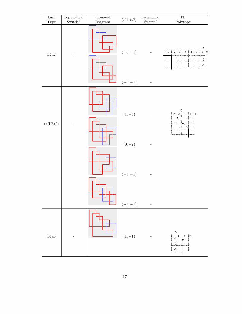
Link Topological Cromwell(𝑡𝑏1, 𝑡𝑏2)

Legendrian TBType Switch? Diagram Switch? Polytope

L7a2 -(−6,−1) - -7 -6 -5 -4 -3 -2 -1 0

-3

-2

-1

0

�

(−6,−1) -

m(L7a2) -

(1,−3) - -2 -1 0 1 2

-4

-3

-2

-1

0

�

�

�

(0,−2) -

(−1,−1) -

(−1,−1) -

L7a3 - (1,−1) - -1 0 1 2

-3

-2

-1

0

�

67

Link Topological Cromwell(𝑡𝑏1, 𝑡𝑏2)

Legendrian TBType Switch? Diagram Switch? Polytope

m(L7a3) -

(−6,−3) - -9 -8 -7 -6 -5 -4 -3 -2 -1 0

-4

-3

-2

-1

0

�

�

�

(−7,−2) -

(−7,−2) -

(−7,−2) -

(−8,−1) -

(−8,−1) -

68

Link Topological Cromwell(𝑡𝑏1, 𝑡𝑏2)

Legendrian TBType Switch? Diagram Switch? Polytope

L7a4 ✓ (−1,−1) ✓ -3 -2 -1 0

-3

-2

-1

0

�

(−1,−1) ✓

m(L7a4) ✓(−4,−3) - -7 -6 -5 -4 -3 -2 -1 0

-7

-6

-5

-4

-3

-2

-1

0

�

�

�

�

�

�(−5,−2) -

(−6,−1) -

L7a5 ✓ (−3,−2) - -5 -4 -3 -2 -1 0

-5

-4

-3

-2

-1

0

�

�

�

�

(−4,−1) -

69

Link Topological Cromwell(𝑡𝑏1, 𝑡𝑏2)

Legendrian TBType Switch? Diagram Switch? Polytope

m(L7a5) ✓(−2,−2) ✗?11 -4 -3 -2 -1 0

-4

-3

-2

-1

0

�

�

�

(−2,−2) ✗?10

(−3,−1) -

(−3,−1) -

L7a6 ✓ (−1,−1) ✗ -3 -2 -1 0

-3

-2

-1

0

�

70

Link Topological Cromwell(𝑡𝑏1, 𝑡𝑏2)

Legendrian TBType Switch? Diagram Switch? Polytope

m(L7a6) ✓

(−4,−3) - -7 -6 -5 -4 -3 -2 -1 0

-7

-6

-5

-4

-3

-2

-1

0

�

�

�

�

�

�(−4,−3) -

(−5,−2) -

(−5,−2) -

(−6,−1) -

L7n1 - (−6,−1) - -7 -6 -5 -4 -3 -2 -1 0

-3

-2

-1

0

�

71

Link Topological Cromwell(𝑡𝑏1, 𝑡𝑏2)

Legendrian TBType Switch? Diagram Switch? Polytope

m(L7n1) - (1,−1) - -1 0 1 2

-3

-2

-1

0

�

L7n2 - (−6,−1) - -7 -6 -5 -4 -3 -2 -1 0

-3

-2

-1

0

�

m(L7n2) - (1,−1) - -1 0 1 2

-3

-2

-1

0

�

L8n1 -(−3,−1) - -4 -3 -2 -1 0

-3

-2

-1

0

�

(−3,−1) -

72

Link Topological Cromwell(𝑡𝑏1, 𝑡𝑏2)

Legendrian TBType Switch? Diagram Switch? Polytope

m(L8n1) - (−3,−1) - -4 -3 -2 -1 0

-3

-2

-1

0

�

L8n2 - (−3,−1) - -4 -3 -2 -1 0

-3

-2

-1

0

�

m(L8n2) - (−3,−1) - -4 -3 -2 -1 0

-3

-2

-1

0

�

L9n1 - (−8,−1) - -9 -8 -7 -6 -5 -4 -3 -2 -1 0

-3

-2

-1

0

�

73

Link Topological Cromwell(𝑡𝑏1, 𝑡𝑏2)

Legendrian TBType Switch? Diagram Switch? Polytope

m(L9n1)- (1,−1) - 0 1 2

-3

-2

-1

0

�

(1,−1) -

L9n2 - (−8,−1) - -9 -8 -7 -6 -5 -4 -3 -2 -1 0

-3

-2

-1

0

�

m(L9n2)- (1,−1) - 0 1 2

-3

-2

-1

0

�

(1,−1) -

(1,−1) -

L9n3 - (−8,−1) - -9 -8 -7 -6 -5 -4 -3 -2 -1 0

-3

-2

-1

0

�

74

Link Topological Cromwell(𝑡𝑏1, 𝑡𝑏2)

Legendrian TBType Switch? Diagram Switch? Polytope

m(L9n3)- (1,−1) - 0 1 2

-3

-2

-1

0

�

(1,−1) -

L9n4- (−10,−1) - -11 -10 -9 -8 -7 -6 -5 -4 -3 -2 -1 0

-3

-2

-1

0

�

(−10,−1) -

m(L9n4) - (3,−1) - 0 1 2 3 4

-3

-2

-1

0

�

L9n5- (−10,−1) - -11 -10 -9 -8 -7 -6 -5 -4 -3 -2 -1 0

-3

-2

-1

0

�

(−10,−1) -

75

Link Topological Cromwell(𝑡𝑏1, 𝑡𝑏2)

Legendrian TBType Switch? Diagram Switch? Polytope

m(L9n5) - (3,−1) - 0 1 2 3 4

-3

-2

-1

0

�

L9n6- (−10,−1) - -11 -10 -9 -8 -7 -6 -5 -4 -3 -2 -1 0

-3

-2

-1

0

�

(−10,−1) -

(−10,−1) -

m(L9n6) - (3,−1) - 0 1 2 3 4

-3

-2

-1

0

�

L9n7- (−8,−1) - -9 -8 -7 -6 -5 -4 -3 -2 -1 0

-3

-2

-1

0

�

(−8,−1) -

76

Link Topological Cromwell(𝑡𝑏1, 𝑡𝑏2)

Legendrian TBType Switch? Diagram Switch? Polytope

m(L9n7)- (1,−1) - 0 1 2

-3

-2

-1

0

�

(1,−1) -

L9n8- (−8,−1) - -9 -8 -7 -6 -5 -4 -3 -2 -1 0

-3

-2

-1

0

�

(−8,−1) -

m(L9n8)- (1,−1) - 0 1 2

-3

-2

-1

0

�

(1,−1) -

L9n9 - (−8,−1) - -9 -8 -7 -6 -5 -4 -3 -2 -1 0

-3

-2

-1

0

�

77

Link Topological Cromwell(𝑡𝑏1, 𝑡𝑏2)

Legendrian TBType Switch? Diagram Switch? Polytope

m(L9n9) - (1,−1) - 0 1 2

-3

-2

-1

0

�

L9n10 ✗(−1,−1) - -3 -2 -1 0

-3

-2

-1

0

�

(−1,−1) -

m(L9n10) ✗

(−3,−4) - -7 -6 -5 -4 -3 -2 -1 0

-5

-4

-3

-2

-1

0

�

�

�

�

(−4,−3) -

(−4,−3) -

(−5,−2) -

78

Link Topological Cromwell(𝑡𝑏1, 𝑡𝑏2)

Legendrian TBType Switch? Diagram Switch? Polytope

m(L9n10)

(−5,−2) -

(−5,−2) -

(−6,−1) -

(−6,−1) -

(−6,−1) -

(−6,−1) -

79

Link Topological Cromwell(𝑡𝑏1, 𝑡𝑏2)

Legendrian TBType Switch? Diagram Switch? Polytope

L9n11 ✗

(−3,−2) -?

(−4,−1) -

(−2,−4) -

m(L9n11) ✗

(−1,−3) - -4 -3 -2 -1 0

-4

-3

-2

-1

0

�

�

�

(−1,−3) -

(−2,−2) -

(−3,−1) -

(−3,−1) -

80

Link Topological Cromwell(𝑡𝑏1, 𝑡𝑏2)

Legendrian TBType Switch? Diagram Switch? Polytope

L9n12 - (3,−1) - 0 1 2 3 4

-3

-2

-1

0

�

m(L9n12) - (−10,−1) - -11 -10 -9 -8 -7 -6 -5 -4 -3 -2 -1 0

-3

-2

-1

0

�

L9n13 ✓(−3,−3) ✗?10 -6 -5 -4 -3 -2 -1 0

-6

-5

-4

-3

-2

-1

0

�

�

�

�

�

(−4,−2) -

(−5,−1) -

(−5,−1) -

81

Link Topological Cromwell(𝑡𝑏1, 𝑡𝑏2)

Legendrian TBType Switch? Diagram Switch? Polytope

m(L9n13) ✓ (−2,−1) - -3 -2 -1 0

-3

-2

-1

0

�

�

L9n14 -

(1,−3) - -2 -1 0 1 2

-4

-3

-2

-1

0

�

�

�

(0,−2) -

(−1,−1) -

(−1,−1) -

m(L9n14) - (−6,−1) - -7 -6 -5 -4 -3 -2 -1 0

-3

-2

-1

0

�

82

Link Topological Cromwell(𝑡𝑏1, 𝑡𝑏2)

Legendrian TBType Switch? Diagram Switch? Polytope

L9n15- (−7,−1) - -8 -7 -6 -5 -4 -3 -2 -1 0

-3

-2

-1

0

�

�

(−6,−2) -

m(L9n15) - (1,−1) - 0 1 2

-3

-2

-1

0

�

L9n16 -(1,−3) - -2 -1 0 1 2

-4

-3

-2

-1

0

�

�

�

(0,−2) -

(−1,−1) -

m(L9n16) - (−6,−1) - -7 -6 -5 -4 -3 -2 -1 0

-3

-2

-1

0

�

83

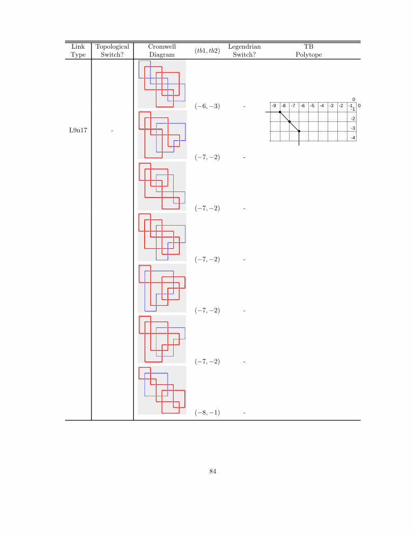
Link Topological Cromwell(𝑡𝑏1, 𝑡𝑏2)

Legendrian TBType Switch? Diagram Switch? Polytope

L9n17 -

(−6,−3) - -9 -8 -7 -6 -5 -4 -3 -2 -1 0

-4

-3

-2

-1

0

�

�

�

(−7,−2) -

(−7,−2) -

(−7,−2) -

(−7,−2) -

(−7,−2) -

(−8,−1) -

84

Link Topological Cromwell(𝑡𝑏1, 𝑡𝑏2)

Legendrian TBType Switch? Diagram Switch? Polytope

m(L9n17)- (1,−1) - 0 1 2

-3

-2

-1

0

�

(1,−1) -

L9n18 ✓(−3,−3) ✓ -8 -7 -6 -5 -4 -3 -2 -1 0

-8

-7

-6

-5

-4

-3

-2

-1

0

�

�

�

�

�

(−5,−2) -

(−7,−1) -

m(L9n18) ✓ (−1,−1) ✓ -3 -2 -1 0

-3

-2

-1

0

�

85

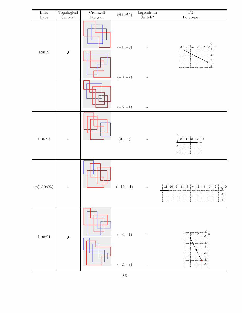
Link Topological Cromwell(𝑡𝑏1, 𝑡𝑏2)

Legendrian TBType Switch? Diagram Switch? Polytope

L9n19 ✗

(−1,−3) - -6 -5 -4 -3 -2 -1 0

-4

-3

-2

-1

0

�

�

�

(−3,−2) -

(−5,−1) -

L10n23 - (3,−1) - 0 1 2 3 4

-3

-2

-1

0

�

m(L10n23) - (−10,−1) - -11 -10 -9 -8 -7 -6 -5 -4 -3 -2 -1 0

-3

-2

-1

0

�

L10n24 ✗(−3,−1) - -4 -3 -2 -1 0

-6

-5

-4

-3

-2

-1

0

�

�

�

(−2,−3) -

86

Link Topological Cromwell(𝑡𝑏1, 𝑡𝑏2)

Legendrian TBType Switch? Diagram Switch? Polytope

m(L10n24) ✗

(−1,−4) - -5 -4 -3 -2 -1 0

-5

-4

-3

-2

-1

0

�

�

�

�

(−1,−4) -

(−2,−3) -

(−3,−2) -

(−3,−2) -

(−4,−1) -

L10n34 - (1,−1) - 0 1 2

-3

-2

-1

0

�

87

Link Topological Cromwell(𝑡𝑏1, 𝑡𝑏2)

Legendrian TBType Switch? Diagram Switch? Polytope

m(L10n34) -(−6,−3) - -9 -8 -7 -6 -5 -4 -3 -2 -1 0

-4

-3

-2

-1

0

�

�

�

(−7,−2) -

(−8,−1) -

L10n42 -(1,−1) - 0 1 2

-3

-2

-1

0

�

(1,−1) -

m(L10n42) -(−6,−3) - -9 -8 -7 -6 -5 -4 -3 -2 -1 0

-4

-3

-2

-1

0

�

�

�

(−7,−2) -

(−8,−1) -

88

Link Topological Cromwell(𝑡𝑏1, 𝑡𝑏2)

Legendrian TBType Switch? Diagram Switch? Polytope

L10n44 ✓

(−4,−3) - -7 -6 -5 -4 -3 -2 -1 0

-7

-6

-5

-4

-3

-2

-1

0

�

�

�

�

�

�(−4,−3) -

(−5,−2) -

(−5,−2) -

(−6,−1) -

(−6,−1) -

m(L10n44) ✓ (−1,−1) ✗?10 -3 -2 -1 0

-3

-2

-1

0

�

89

Link Topological Cromwell(𝑡𝑏1, 𝑡𝑏2)

Legendrian TBType Switch? Diagram Switch? Polytope

L10n45 -(−3,−2) - -5 -4 -3 -2 -1 0

-3

-2

-1

0

�

�

(−4,−1) -

m(L10n45) -(−3,−1) - -4 -3 -2 -1 0

-3

-2

-1

0

�

(−3,−1) -

L10n46 - (−3,−1) - -4 -3 -2 -1 0

-3

-2

-1

0

�

L10n54 ✓ (−1,−1) ✗?10 -3 -2 -1 0

-3

-2

-1

0

�

90

Link Topological Cromwell(𝑡𝑏1, 𝑡𝑏2)

Legendrian TBType Switch? Diagram Switch? Polytope

m(L10n54) ✓ (−4,−3) - -9 -8 -7 -6 -5 -4 -3 -2 -1 0

-9

-8

-7

-6

-5

-4

-3

-2

-1

0

�

�

�

�

�

�

(−6,−2) -

L10n56 ✗

(−4,−3) -?

(−6,−2) -

(−3,−5) -

m(L10n56) ✗ (−1,−1) - -3 -2 -1 0

-3

-2

-1

0

�

91

Link Topological Cromwell(𝑡𝑏1, 𝑡𝑏2)

Legendrian TBType Switch? Diagram Switch? Polytope

L10n57 ✗(−4,−1) -

?

(−3,−3) -

m(L10n57) ✗ (−3,−1) - ?

L11n119 - (3,−1) - 0 1 2 3 4

-3

-2

-1

0

�

m(L11n119) - (−10,−1) - -11 -10 -9 -8 -7 -6 -5 -4 -3 -2 -1 0

-3

-2

-1

0

�

L11n132 - (−10,−1) - -11 -10 -9 -8 -7 -6 -5 -4 -3 -2 -1 0

-3

-2

-1

0

�

92

Link Topological Cromwell(𝑡𝑏1, 𝑡𝑏2)

Legendrian TBType Switch? Diagram Switch? Polytope

m(L11n132) -(3,−1) - 0 1 2 3 4

-3

-2

-1

0

�

(3,−1) -

L11n133 - (−10,−1) - -11 -10 -9 -8 -7 -6 -5 -4 -3 -2 -1 0

-3

-2

-1

0

�

m(L11n133) - (3,−1) - 0 1 2 3 4

-3

-2

-1

0

�

L11n139 -(1,−1) - 0 1 2

-3

-2

-1

0

�

(1,−1) -

93

Link Topological Cromwell(𝑡𝑏1, 𝑡𝑏2)

Legendrian TBType Switch? Diagram Switch? Polytope

m(L11n139) - (−8,−1) - -9 -8 -7 -6 -5 -4 -3 -2 -1 0

-3

-2

-1

0

�

L11n140 - (−8,−1) - -9 -8 -7 -6 -5 -4 -3 -2 -1 0

-3

-2

-1

0

�

m(L11n140) -

(1,−1) - 0 1 2

-3

-2

-1

0

�

(1,−1) -

(1,−1) -

(1,−1) -

94

Link Topological Cromwell(𝑡𝑏1, 𝑡𝑏2)

Legendrian TBType Switch? Diagram Switch? Polytope

L11n148 - (1,−1) - 0 1 2

-3

-2

-1

0

�

m(L11n148) - (−8,−1) - -9 -8 -7 -6 -5 -4 -3 -2 -1 0

-3

-2

-1

0

�

L11n204 -(−6,−3) - -10 -9 -8 -7 -6 -5 -4 -3 -2 -1 0

-4

-3

-2

-1

0

�

�

�

(−7,−2) -

(−9,−1) -

m(L11n204) - (1,−1) - 0 1 2

-3

-2

-1

0

�

95

Link Topological Cromwell(𝑡𝑏1, 𝑡𝑏2)

Legendrian TBType Switch? Diagram Switch? Polytope

L11n205 - (−6,−1) - -7 -6 -5 -4 -3 -2 -1 0

-3

-2

-1

0

�

m(L11n205) - (1,−3) - -4 -3 -2 -1 0 1 2

-4

-3

-2

-1

0

�

�

�

L11n218 -(1,−3) -

?

(−1,−2) -

m(L11n218) - (−6,−1) - -7 -6 -5 -4 -3 -2 -1 0

-3

-2

-1

0

�

96

Link Topological Cromwell(𝑡𝑏1, 𝑡𝑏2)

Legendrian TBType Switch? Diagram Switch? Polytope

L11n219 -(1,−3) -

?

(−1,−2) -

m(L11n219) - (−6,−1) - -7 -6 -5 -4 -3 -2 -1 0

-3

-2

-1

0

�

L11n226 -(−6,−3) -

?

(−8,−2) -

m(L11n226) - (1,−1) - 0 1 2

-3

-2

-1

0

�

97