classifying north atlantic tropical cyclone tracks by mass

Classifying North Atlantic Tropical Cyclone Tracks by Mass Moments*

JENNIFER NAKAMURA

Lamont-Doherty Earth Observatory, Columbia University, Palisades, New York

UPMANU LALL

Department of Earth and Environmental Engineering, Columbia University, New York, New York

YOCHANAN KUSHNIR AND SUZANA J. CAMARGO

Lamont-Doherty Earth Observatory, Columbia University, Palisades, New York

(Manuscript received 4 September 2008, in final form 12 May 2009)

ABSTRACT

A new method for classifying tropical cyclones or similar features is introduced. The cyclone track is

considered as an open spatial curve, with the wind speed or power information along the curve considered to

be a mass attribute. The first and second moments of the resulting object are computed and then used to

classify the historical tracks using standard clustering algorithms. Mass moments allow the whole track shape,

length, and location to be incorporated into the clustering methodology. Tropical cyclones in the North

Atlantic basin are clustered with K-means by mass moments, producing an optimum of six clusters with

differing genesis locations, track shapes, intensities, life spans, landfalls, seasonal patterns, and trends. Even

variables that are not directly clustered show distinct separation between clusters. A trend analysis confirms

recent conclusions of increasing tropical cyclones in the basin over the past two decades. However, the trends

vary across clusters.

1. Introduction

Tropical cyclones lead to major natural disasters in the

regions of landfall with devastating storm surges, flooding,

and high winds. Named storms (NS) include all tropical

cyclones reaching a maximum sustained wind speed of

at least 18 m s21 (35 kt) (Neumann et al. 1993). Their

impact along the Atlantic coast of North and Central

America is often catastrophic to life, ecology, property,

wetlands, and coastal estuaries [e.g., in 1995 total main-

land U.S. tropical cyclone damage averaged on the order

of $5 billion; see Pielke and Landsea (1998)]. The severity

and frequency of NS is consequently of great interest

for disaster planning and mitigation. Determining the

spatial characteristics of tropical cyclone frequency and

intensity is of considerable importance for any study of

past, present, and future hurricane impact or model val-

idation. Clustering provides a way to assess the congru-

ence in spatial characteristics such as track shape, genesis

location, intensity, life span, seasonality, and landfall.

The causal factors associated with each cluster, as well

as the ability of numerical simulation models to simulate

the frequency of each cluster, conditional on specified

boundary conditions, could then be assessed. Macrolevel

statistics of the conditional dependence of each cluster on

antecedent conditions could also be assessed.

To a first approximation, hurricanes move in the di-

rection that the mean tropospheric winds (over the

depth of the storm) steer them. In the northern Atlantic,

the northeasterly trade winds move the storms westward

from the African coast. The prevailing flow around the

subtropical high curves them northward approaching

the North American coast and eastward in the middle

latitudes. Elsner and Kara (1999) call this track shape

the parabolic sweep. The position and strength of the

subtropical high, the extratropical circulation, and the

* Lamont-Doherty Earth Observatory Contribution Number

7295.

Corresponding author address: Jennifer Nakamura, Lamont-

Doherty Earth Observatory, The Earth Institute at Columbia

University, 61 Rte. 9W, Palisades, NY 10964.

E-mail: [email protected]

15 OCTOBER 2009 N A K A M U R A E T A L . 5481

DOI: 10.1175/2009JCLI2828.1

� 2009 American Meteorological Society

genesis location of the hurricane vary, allowing variation

in track shape and length. Genesis location can be linked

to the seasonality, sea surface temperature, wind shear,

and position of the initial disturbance (Gray 1968, 1979;

Henderson-Sellers et al. 1998). Both maximum wind

speed (or intensity) and life span are linked to the genesis

location and track shape as some locations/curvatures

provide a longer time to intensify before encountering

land or colder water. Landfall and the intensity of the

storm at landfall are also associated with genesis loca-

tion and track shape (Camargo et al. 2007).

Cluster analysis provides a way to objectively classify

storms in a given ocean basin into subcategories depend-

ing on geographical properties of the storms (e.g., genesis,

track location, and shape). Such classification can become

useful for building predictive understanding on climate

time scales. The K-means method (MacQueen 1967) is a

common clustering method that has been used both with

tropical (Elsner and Liu 2003; Elsner 2003) and extra-

tropical cyclone tracks (Blender et al. 1997). The method

is typically applied to vector data on select attributes

and seeks to find k separations of the data such that the

intercluster variation is maximized relative to the centroid

of each cluster in the space formed by the vectors sub-

mitted. The application of this method to hurricane tracks

(potentially specified as vectors defined by the x and y

coordinates of the track) also faces the challenge that the

tracks, and hence the data vectors with track coordinates,

are of unequal lengths. The studies referenced above ad-

dressed this problem by using two points along the track

(positions of maximum and final hurricane intensities), or

dimensional vectors (centroids of the cyclone trajectories

every 6 h for the first 3 days), respectively.

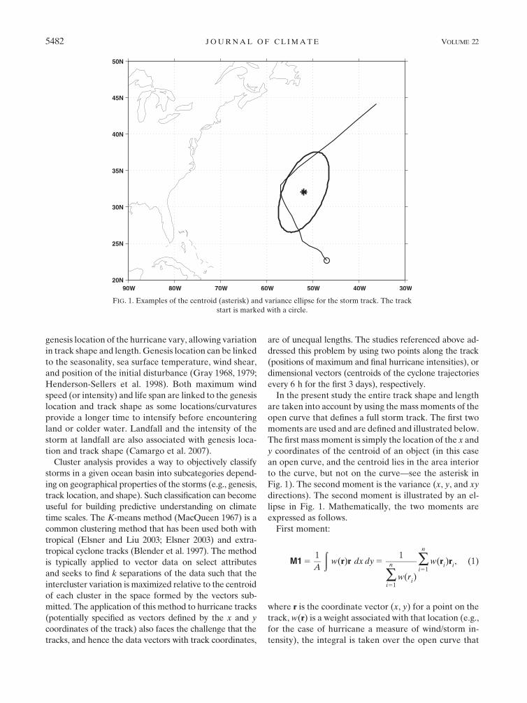
In the present study the entire track shape and length

are taken into account by using the mass moments of the

open curve that defines a full storm track. The first two

moments are used and are defined and illustrated below.

The first mass moment is simply the location of the x and

y coordinates of the centroid of an object (in this case

an open curve, and the centroid lies in the area interior

to the curve, but not on the curve—see the asterisk in

Fig. 1). The second moment is the variance (x, y, and xy

directions). The second moment is illustrated by an el-

lipse in Fig. 1. Mathematically, the two moments are

expressed as follows.

First moment:

M1 51

A

ðw(r)r dx dy 5

1

�n

i51w(r

i)

�n

i51w(r

i)r

i, (1)

where r is the coordinate vector (x, y) for a point on the

track, w(r) is a weight associated with that location (e.g.,

for the case of hurricane a measure of wind/storm in-

tensity), the integral is taken over the open curve that

FIG. 1. Examples of the centroid (asterisk) and variance ellipse for the storm track. The track

start is marked with a circle.

5482 J O U R N A L O F C L I M A T E VOLUME 22

defines the track, A is a normalization constant that re-

flects the total intensity over the track, and the sum on

the right-hand side of the equation defines the discrete

approximation to the integral over the track, using the n

recorded locations of the track over the lifetime of the

storm.

Second moment:

M2 51

A

ðw(r)(r�M1)2 dx dy

51

�n

i51w(r

i)

�n

i51w(r

i)(r

i�M1

i)2, (2)

where M1, r, w(r), A, and n are defined as in the first

moment. In matrix format, the variance is the covariance

matrix between the scalar components (x and y) of r giving

three directions to the second moment of x, y, and xy.

These five numbers (two centroid and three covari-

ance) then constitute the summary of the track infor-

mation that is to be used to identify track clusters. The

first moment establishes the location of the effective

center of gravity of the storm track, while the second

moment provides a measure of the shape of the storm.

The classical covariance measure is usually explained as

a measure of the orientation and length of the principal

axes of an ellipse that describes the scatter of data in a

plane. A similar interpretation applies here, with the

qualification that the data of interest is not a scatterplot,

but a section of a curve that is being approximated as an

ellipse. Thus, if two tracks were perfect straight lines but

with different lengths, then the second-moment matrix

would identify the same orientation for both of them,

but with a different spread along that direction. If the

first track is a straight line and the other part of an el-

lipse, then from the covariance ellipse we would see that

the length of the second principal axis is zero, indicating

that there is no variation in that direction, while it would

be nonzero for the curve, the magnitude increasing as

the relative curvature increases. Further, if both tracks

are curves, but one is convex and the other concave with

respect to a particular reference frame, then the signs of

the cross-covariance terms in the second-moment ma-

trix are opposite, and one can recognize this condition.

Thus, using the first two moments of a storm track one

can get a measure of its central location, length, orien-

tation, and also curvature. This allows one to get an

approximation for most of the typical tracks that we

observe. Complex features, such as tracks that curve

back onto themselves or are concave in some sections

and convex in others will require recourse to higher

moments.

The analysis of the track moments is performed here

not during the evolution of a track but postmortem,

taking into account the whole life cycle. Hence, this

approach will not be useful for describing an evolving

storm. Rather, it is intended for an analysis of historical

data, especially for the identification of trends and as-

sociated causal factors for particular types of storms.

The dataset used is described in the next section

along with some aspects of the clustering methodology.

Section 3 presents associated results for northern At-

lantic tropical storms, including a discussion of the attri-

butes of the clusters in terms of spatial characteristics

such as track shape, genesis location, intensity, life span,

seasonality, and landfall. The last section compares our

results with those from a selection of other methods.

2. Data

Atlantic basin historical hurricane track data

(HURDAT), with information on storm position

(latitude–longitude) every 6 hours available from the

National Hurricane Center (NHC), was used. Only NS

from 1948 to 2006 were retained for our analysis. Owing

to routine aircraft reconnaissance missions into tropical

cyclones beginning in 1944, details on the position of

the hurricane structure are available. This has lead to

greater accuracy in the 6-h position data.

Clustering methodology

A variety of methods for the identification of clusters

from vector data are available. Here, we use the K-means

method with a vector of five attributes per track: two for

latitudinal and longitudinal centroids and three for the

variance (latitudinal, longitudinal, and diagonal).

FIG. 2. (top) Mean silhouette values and (bottom) number of

negative silhouette values.


The variance components contain much larger values

than the centroid components. To give the centroid and

variance equal weight in the cluster analysis, the vari-

ables are standardized (to mean zero and first standard

deviation); each centroid column is multiplied by 0.5/2,

and each variance column by 0.5/3 so that the centroid

and the covariance are treated roughly on par as to

their importance for clustering. Other weights that

emphasize one or the other attribute could indeed be

chosen.

Moments along the northern Atlantic cyclone tracks

were estimated using wind velocity (or power) recorded

along the track as a weight and also using uniform

weights [w(r) of ones in 1 and 2]. Each of the resulting

data was then used in K-means cluster analysis. Results

are presented for the uniform weight case. Separation

between the clusters was distinct and clusters cohesive as

tracks were grouped together in geographical regions.

When wind velocity weights are used, tracks farther

apart are added to the cluster.

The K-means clustering algorithm partitions the data

into k clusters, with cluster centroids denoted by mi and

coordinates as xi,j, such that the variance across clusters

defined below is maximized; J is the index over all points

in cluster i (i 5 1 . . . k):

var 5 �k

i51�

l

j51(x

i,j� m

i)2. (3)

The K-means cluster analysis package available in Mat-

lab 7.3 considers multiple runs with random seeding of

clusters. The optimal cluster number j is determined by

the maximum mean and minimum number of negative

FIG. 3. Centroid locations (asterisks) and directional variance (light ellipses) for the six clusters. The

mean centroid value is marked with a dark x, and the mean variance ellipse with a dark line.

TABLE 1. Mean centroid and variance values for each cluster.

Cluster

Centroid x

(8W)

Centroid y

(8N)

Variance

x

Variance

y

Variance

xy

1 58.38 25.69 168.25 128.29 247.89

2 65.68 34.07 67.20 36.33 33.99

3 43.06 29.06 41.89 50.48 5.64

4 58.83 16.16 75.28 9.34 214.98

5 55.20 55.20 381.27 129.95 171.38

6 87.32 25.15 21.74 15.57 22.48


‘‘silhouette’’ values. A silhouette is both a measure of

how cohesive each cluster is and how well the clusters are

separated. For i total points a silhouette (Si) is defined as

Si5

min(bi)� a

i

max[ai, min(b

i)]

, (4)

where ai is the average distance from the ith point to the

other points within the cluster and bi is the average

distance from the ith point to points in another cluster

(Kaufman and Rousseeuw 1990). Silhouette values

range from 21 to 1. Clusters with a high mean silhouette

value are cohesive and negative silhouette values are

possible misclassified points. Figure 2 shows the mean

silhouette values (top) and number of negative silhou-

ette values (bottom) for a selected run with the northern

Atlantic hurricane data. Cluster numbers from two to

nine run along the x axis. Note that the mean silhouette

value for the six clusters is a maximum in the top panel

of Fig. 2 and the number of negative silhouette values a

minimum in the bottom panel, indicating the best choice

of cluster number is six.

3. Cluster analysis results

a. Centroids and variance

The actual output of the K-means clustering is groups

of centroid locations and directional variance (Fig. 3).

Clear separation of the clusters can be seen in the

groupings of the centroids and slope and size of the

variance ellipses. The mean centroid value is marked

with a dark x, and mean variance ellipse with a dark line.

Table 1 presents the mean centroid location and direc-

tional variance for each cluster (1–6). Cluster 1 is centered

FIG. 4. Genesis location (circle) and the track (line) for the six clusters.

TABLE 2. Mean and range of tropical cyclone genesis locations for

each cluster.

Cluster

Mean x

genesis (8W)

Mean y

genesis (8N)

Genesis x

range (8W)

Genesis y

range (8N)

1 34.60 12.61 77–18 7.2–18.2

2 70.50 26.64 96–44 11.7–44

3 39.35 20.76 68.8–17.4 8.6–42.5

4 46.83 12.76 81.6–14 8.4–24

5 65.89 20.67 96.2–20.5 10.9–34.3

6 83.16 20.77 97–50.5 10–32


just west of midbasin with rounded variance ellipses (the

mean variance x is approximately equal to mean vari-

ance y) and a slightly negative tilt (negative mean vari-

ance xy). The mean location of cluster 2 is slightly higher

than that of cluster 1 near the eastern coast of the United

States. The variance ellipses are elongated along the x

axis with a positive tilt. Cluster 3 sits midbasin with

rounded ellipses and nearly zero tilt. The farthest

southern cluster is 4 and its ellipses are stretched along

the x axis with a slightly negative tilt. The farthest north

of all clusters is 5. It also has the largest ellipses, elon-

gated along the x axis and heavily positively tilted.

Cluster 6 is centered over the Gulf of Mexico and, like

cluster 3, is rounded with near-zero tilt; it has the

smallest variance ellipses.

b. Genesis location and track shape

Although the track location and shape are taken into

account with the centroid and variance, the first reported

location or genesis and actual track are not directly used

in the entire analysis. Still, clear groupings can be seen in

Fig. 4 with the genesis location as a circle and the track as

a line. Table 2 presents the mean genesis location in each

cluster along with the range of those first positions.

Cluster 1 genesis locations fall roughly within the main

development region of Goldenberg et al. (2001). These

are Cape Verde hurricanes [Atlantic basin hurricanes

that form close to the Cape Verde Islands (,1000 km)

and become tropical cyclones before reaching the Ca-

ribbean] moving in a classic parabolic shape as described

by Elsner and Kara (1999). They are the tropical cy-

clones forming farthest east of all the clusters and have

the smallest genesis range in latitude. The tropical cy-

clones forming farthest north are in cluster 2. They have

a diffuse genesis range in both latitude and longitude and

move along the eastern coast of the United States. The

largest genesis range in latitude is found in cluster 3 and

these storms follow a flattened-shape parabola. The

genesis location of cluster 4 resembles cluster 1 with a

small genesis range in latitude in the Cape Verde region.

What differentiates these tropical cyclones is the nearly

straight track shape: they rarely venture above 258N. The

most diffuse in genesis location is cluster 5, with the

largest genesis range in longitude. The tropical cyclones

in cluster 5 are not full parabolas, but rather partial

‘‘hooks’’ or semiparabolas. Cluster 6 genesis locations

are confined to the Gulf of Mexico and Caribbean, with

the smallest genesis range in longitude. These tropical

cyclones also tend to stay in the gulf.

c. Intensity and life span

The life span of a storm usually affects the size of the

variance ellipse; that is, a longer track equals a larger

ellipse unless the tropical cyclone is very slow moving.

FIG. 5. The 25th and 75th percentiles (upper and lower bounds of the box), the mean (as-

terisk), the median (bar in middle), the bounds (dashed line), and outliers (plus signs) of the

distribution of tropical cyclone maximum wind speed in each cluster and as a whole.


The next three figures, which explore the maximum wind

speed (Fig. 5), life span (Fig. 6), and maximum intensity

(Fig. 7), are box plots. These illustrate the 25th and 75th

percentiles (upper and lower bounds of the box), the

mean (asterisk), the median (bar in middle), the bounds

(dashed line), and outliers (plus signs) of the distribution

of tropical cyclones in each cluster and as a whole.

Maximum wind speed is categorized by the Saffir–

Simpson scale as follows: tropical storm (TS), 35–64 kt;

Category 1, 65–82 kt; Category 2, 83–95 kt; Category 3,

96–113 kt; Category 4, 114–135 kt; and Category 5,

greater than 135 kt. Figure 5 shows the maximum wind

speed in knots of the six clusters and all tropical cyclones.

Table 3 presents the mean and median categories of the

maximum wind speed. Cluster 1 is considerably stronger

than the other clusters and the total, with cluster 5 coming

in second. Clusters 2 and 3 are only slightly weaker than

the total mean, keeping within the same category. Clus-

ters 6 and 4 are weaker than the total with the median

maximum wind speed falling in the TS category. The

strongest, cluster 1, shows a negative skew distribution as

compared to normal with the median in a higher category

than the mean (majority of storms weaker than the

mean) and the weakest, clusters 4 and 6, show a positive

skew with the median in a lower category than the mean

(majority of storms stronger than the mean).

Life span was converted from 6-h periods to days

for easier viewing in Fig. 6. If ranked from longest

to shortest, it follows the same pattern as the maxi-

mum wind speed except for the last two, which are

nearly equal. The three longest clusters (1, 5, and 3) are

longer than the total and the three shortest (2, 4, and 6)

are shorter. The longer the life span, the longer the

time the tropical cyclone has to intensify as long as the

conditions stay favorable (i.e., warm waters and low

shear). Life spans were all negatively skewed with the

majority of the tropical cyclones lasting less time than

the mean.

The power dissipation index (PDI) (Emanuel 2005) is

a hybrid of the maximum wind speed and the life span

and is used here as a measure of integrated intensity.

Emanuel (2007) found the index to covary with low-level

vorticity and vertical wind shear and correlate highly with

sea surface temperature. PDI is defined as the simplified

power dissipation index, as in Emanuel (2005):

PDI [

ðn

1

V3 dt, (5)

where n is the number of time steps with dt in seconds and

V is the wind velocity in meters per second giving units

of PDI in cubic meters per second squared. The large

index values are multiplied by 1 3 10211 for plotting ease.

Not surprisingly, the combination of wind speed and life

span shows cluster 1 to be the most intense, followed by

cluster 5. These are the only two that are stronger than

FIG. 6. As in Fig. 5, but for the life span (days) in each cluster and as a whole.


the average of all. However, the distributions of clusters

2–6 show quite a few outliers, indicating that intense

storms are possible in these clusters, but more of a rare

event than for cluster 1. All the distributions are nega-

tively skewed, just like the life spans, indicating that the

majority of tropical cyclones are less intense than the

mean.

d. Seasonality

If following the mariner’s poem (Inwards 1898, p. 86),

June too soon.July stand by.August look out you must.September remember.October all over.

one would conclude that the North Atlantic hurricane

season is four months long, from July through October.

Indeed, looking at a box plot of storm month (Fig. 8) and

not counting outliers, three of the clusters (1, 3, and 6)

along with all storms show a four-month season from

July to October. However, two clusters have a six-month

season (4 and 5) from June through November and

cluster 2 has an eight-month season from April through

November. Outliers even show a tropical cyclone in

February. Note that, due to the discrete nature of the

month, sometimes the 25th or the 75th percentile and

the median are the same, so for Fig. 8 the median is

marked with a circle. The cluster means all fall in August

(eight) and September (nine) with two medians in Au-

gust (clusters 1 and 2), and the rest in September: Sep-

tember is to remember. Three clusters have a negative

skew with more tropical cyclones occurring earlier than

the mean (1, 2, and 3), and the other three along with the

total having a positive skew with more occurring later

than the mean.

e. Landfall

Landfall was inferred by applying a 18 land–sea mask

and counting the number of storms that crossed from

ocean to land between 58 and 458N, 1008 and 508W.

Table 4 presents the cluster number, number of tropical

cyclones in each cluster, number of landfalls, and the

FIG. 7. As in Fig. 5, but for the tropical cyclone PDI multiplied by 1 3 10211 in each cluster and

as a whole.

TABLE 3. Mean and median category of the maximum wind speed

in each cluster and in all tropical cyclones.

Cluster Mean Median

1 3 4

2 1 1

3 1 1

4 1 TS

5 2 2

6 1 TS

All 1 1


percentage of landfall. Not only does cluster 6 have the

highest number of storms, it also has the most landfalls.

Tropical cyclones in that cluster do not have far to travel

before they hit land. The most intense tropical cyclones

in cluster 1 have a slightly higher percentage of hitting

land than all storms; however, the number of storms in

that cluster is fairly low. The second most intense storms

in cluster 5 have the smallest number of tropical cy-

clones and a lower than all-storms landfall percentage.

Clusters 2 and 4 both have a smaller landfall percentage

than all storms; however, cluster 2 is well populated.

Cluster 3 storms do not make landfall in the box chosen.

f. Trends

The Poisson distribution is ideally suited to model

tropical cyclone counts as they are relatively rare oc-

curring events. The probability of these rare events

allowing counts per year (Yi) with integer values of y 5

0, 1, 2, . . . , mean m(xi) . 0, and the number of replica-

tions for each observation ni is

P(Yi5 y) 5

[nim(x

i)]y

y!e�nm(x

i). (6)

For the Poisson distribution the mean is also equal to the

variance. A simple generalized linear model for the

mean (variance) that keeps counts positive is a log-linear

model:

u 5 logm(xi). (7)

The global log likelihood of parameter vector u 5 (u(xi),

. . . , u(xn)) is

L(u) 5 �n

i51logf f [Y

i, u(x

i)]g. (8)

Within a smoothing window and taking advantage of

this log link, the local log-likelihood function [product of

probabilities given by Eq. (6)] is

Lx(a) 5 �

n

i51w

i(x)A(x

i� x)Y

i, (9)

where A is a vector of explanatory variables (fitting

functions), a is a vector of the coefficients in a local

FIG. 8. As in Fig. 5, but for the tropical cyclone month in each cluster and as a whole.

TABLE 4. Number of tropical cyclones (N) and landfalls and the

landfall percentage for each cluster and for all tropical cyclones.

Cluster N Landfalls Landfall percentage

1 70 32 46

2 157 35 22

3 94 0 0

4 92 26 28

5 43 14 33

6 174 148 85

All 630 255 40


linear approximation (a0 1 a1x), xi are estimated points,

x are the observed points, and wi is the weight:

wi(x) 5 W

xi� x

h(x)

� �, W 5 (1� juj3)3, juj, 1, (10)

where h(x) is the bandwidth and W is the tricube weight

function with smoothing parameter u.

The numbers of tropical cyclones per year in each

cluster along with the number for the whole basin were

analyzed by using this Poisson local linear log-likelihood

(Fig. 9) by the Matlab version Locfit (Loader 1999).

The fit is made in a moving window (nearest neighbor

method) with 70% of the data (in this case 41 years)

ensuring the local neighborhoods always contain a

specified number of points (Loader 1999). The number

of years runs along the x axis; the count on the y axis with

the cluster name as the y label. All clusters show an

upward trend in the last two decades, but some are more

pronounced than others (clusters 1, 2, 4, and 5). Kossin

et al. (2007) found that a trend for an increase in the NS

counts in 1984–2004 in the North Atlantic basin was well

supported. Goldenberg et al. (2001) also found recent

upward trends in intense hurricanes.

The total PDI per year (multiplied by 1 3 10211) is

plotted as dots with the Poisson local linear log-likelihood

FIG. 9. The number of tropical cyclones per year

in each cluster along with the number for the whole

basin (dots) with the linear Poisson local linear log-

likelihood fit as a line.


as a line in Fig. 10. Year to year the index is highly

variable. Emanuel (2007) found the variability to be

linked to net surface radiation, thermodynamic effi-

ciency, and average surface wind speed. It appears that

the most intense clusters (1 and 5) have the strongest

trend in the last two decades, although the last year

(2006) showed a substantial downturn in cluster 1.

Elsner et al. (2008) found an increased intensity of the

strongest tropical cyclones due to an increase in ocean

temperatures over the Atlantic Ocean and elsewhere.

Both cluster 1 and the total were raised significantly by

Hurricane Ivan in 2004. Ivan not only was a long track,

but quickly intensified to Categories 4 and 5 and oscil-

lated between the two. The all storms plot differs from

Fig. 1 in Emanuel (2005) (Atlantic basin power dissi-

pation index) because of the correction Emanuel ap-

plied to reduce the wind speed in the presatellite era

and smoothing (Emanuel 2005, see the Supplementary

Methods section). Landsea (2005) argues that the re-

duction is unwarranted because ‘‘in major hurricanes

winds are substantially stronger at the ocean’s surface

than previously realized.’’

In summary, the trends for tropical cyclone counts and

PDI vary by cluster. The evidence for linear trends over

the period of record appears weak. However, there is

evidence for an increasing trend in the last decade or so

in both variables. The higher activity and intensity in the

early part of the record is also notable for several of the

FIG. 10. PDI (m3 s22) per year multiplied by

1 3 10211 in each cluster along with the number for

the whole basin (dots) with the linear Poisson local

linear log-likelihood fit as a line.


clusters. The spatial shift in the PDI trends may be

worthy of further investigation.

4. Discussion and conclusions

a. Contrasting other North Atlantic clustering studies

This is not the first study to use K-means clustering on

North Atlantic tropical cyclones. Elsner (2003) clus-

tered by latitude and longitude coordinates at maximum

and final hurricane intensities and found three clusters.

Elsner’s study did not include TS tracks or portions of

tracks resulting in shorter trajectories. Figure 1 of that

paper shows the three clusters. Elsner finds the shorter

trajectory, straight moving cluster (red) to be the most

intense. By including the tropical storm part of the track,

we found the longest tracks to be the most intense

(correlation of 0.68 for length and intensity of all clus-

ters, which is a significant t value for a two-tailed dis-

tribution at the 0.01 level). The three clusters are similar

to the results that we found when only clustering cen-

troids (Fig. 11, top); the cluster regimes have nearly

north–south oriented breaks.

Camargo and Kossin (2008) have also completed pre-

liminary clustering in the North Atlantic, incorporating

the whole track length and actual location by using a

regression mixture model on the entire HURDAT da-

taset. Three clusters were found: the Gulf of Mexico,

Cape Verde, and eastern U.S.-born storms (11 bottom).

When the K-means analysis is redone over a similar time

period (1851–2003) for centroid and variance, the resulting

FIG. 11. Centroid locations of three clusters from 1851 to 2003 for (top) the K-means on

centroids only, (middle) the K-means on the centroid and variance, and (bottom) the Camargo

and Kossin (2008) regression mixture model.


clusters are strikingly similar (Fig. 11, middle). How-

ever, in this method, silhouette values indicate the op-

timal number of clusters to be six. In their North Pacific

paper, Camargo et al. (2007) found a similar result of

longer cyclone life spans leading to more intensification.

The cluster number in these papers is based on an esti-

mation of the diminishing return of log-likelihood plots

and visual analysis. Camargo and Kossin (2008) also

note that their finite mixture model produces better

results than the K-means clustering because they take

into account the whole track shape and location. Mo-

ments allow the use of the simple and computationally

elegant K-means while also taking into account the

whole track shape and location.

b. Summary

A novel approach for clustering storm tracks was

developed using K-means clustering with the mass mo-

ments of centroid and variance. The centroid captures

where the tropical cyclone is located and the variance

describes the entire track shape. A summary of the re-

sults follows.

d A tropical storm track can be thought of as an open

curve allowing computation of the first and second

moments (centroid and variance, see Fig. 1).d The K-means applied to the first two moments for

each track provides a method for selection of clusters

or groups. The group number is selected through the

mean and number of negative silhouette values (Fig. 2).d The resulting clusters (Fig. 3 and Table 1) have not

only grouped centroid locations but also distinctly

differently shaped variance ellipses.

d Although genesis locations of some clusters are diffuse

(clusters 2, 3, and 5; see Table 2), the track shapes

(Fig. 4) clearly follow a pattern: cluster 1 is the classic

parabola, cluster 2 includes U.S. East Coast storms,

cluster 3 the flattened parabolas, cluster 4 includes the

straight-moving storms, cluster 5 the semiparabolas,

and cluster 6 includes the Gulf storms.

d Both maximum wind speed and intensity were found

to be linked to life span (correlations of 0.59 and 0.68,

respectively, over all clusters: significant for a two-

tailed distribution at the 0.01 level) with longer tracks

producing higher maximum wind speeds and more

intense tropical cyclones (Figs. 5–7).d Half of the clusters showed the typical four-month-

long Atlantic tropical storm season from July to Oc-

tober, while two clusters had a longer six-month season

from June to November, and one cluster showed an

eight-month season from April to November (Fig. 8).d Landfall percentages of the clusters were clearly dif-

ferent, ranging from 0% to 85% (Table 4).

d Trends for the number of cyclones per year show an

upward trend over the last two decades, but some are

more pronounced than others (Fig. 9).d Upward trends in maximum intensity of the most in-

tense cyclone clusters were found to be stronger than

those for all storms (Fig. 10).d Results of the Elsner (2003) K-means study using two

points along the track appear to correspond well to

those obtained by only using the first moment of the

tracks in the K-means (Fig. 11, top). Thus, Elsner’s

(2003) method uses only part of the information.d Results of the Camargo and Kossin (2008) regression

mixture model are similar to those obtained using

both first and second moments in K-means (cf. Fig. 11

middle and bottom).

Future work will include exploring the meteorological

conditions behind the six clusters. As tropical cyclone

formation and movement is based on meteorological

conditions, the hypotheses of clusters also being related

is a sensible one. If clear connections are found, then

known meteorological conditions can be linked to a

particular class and shape of storms. Possible risk as-

sessment applications include relating climate fields or

indices to an increased or decreased chance of tropical

cyclone genesis, genesis location, and track shape.

These, in turn, can be related to landfall and possible

landfall intensities, which is of interest to government

planning boards and insurance companies.

Acknowledgments. We wish to thank the reviewers

for constructive comments that improved the paper.

This study was made possible by an Award from the

Columbia University Office of Research Initiatives.

REFERENCES

Blender, R., K. Fraedrich, and F. Lunkeit, 1997: Identification of

cyclone-track regimes in the North Atlantic. Quart. J. Roy.

Meteor. Soc., 123, 727–741.

Camargo, S. J., and J. P. Kossin, 2008: Relationship of the Atlantic

meridional mode with Atlantic hurricane tracks. Preprints,

28th Conf. on Hurricanes and Tropical Meteorology, Orlando,

FL, Amer. Meteor. Soc., P2A2. [Available online at http://

ams.confex.com/ams/pdfpapers/137682.pdf.]

——, A. W. Robertson, S. J. Gaffney, P. Smyth, and M. Ghil, 2007:

Cluster analysis of tropical cyclone tracks. Part I: General

properties. J. Climate, 20, 3635–3653.

Elsner, J. B., 2003: Tracking hurricanes. Bull. Amer. Meteor. Soc.,

84, 353–356.

——, and A. B. Kara, 1999: Hurricanes of the North Atlantic: Cli-

mate and Society. Oxford University Press, 512 pp.

——, and K. B. Liu, 2003: Examining the ENSO-typhoon hy-

pothesis. Climate Res., 25, 43–54.

——, J. P. Kossin, and T. H. Jagger, 2008: The increasing intensity

of the strongest tropical cyclones. Nature, 455, 92–95.


Emanuel, K. A., 2005: Increasing destructiveness of tropical cy-

clones over the past 30 years. Nature, 436, 686–688.

——, 2007: Environmental factors affecting tropical cyclone power

dissipation. J. Climate, 20, 5497–5509.

Goldenberg, S. B., C. W. Landsea, A. M. Mestas-Nunez, and

W. M. Gray, 2001: The recent increase in Atlantic hurricane

activity: Causes and implications. Science, 293, 474–479.

Gray, W. M., 1968: Global view of the origin of tropical distur-

bances and storms. Mon. Wea. Rev., 96, 669–697.

——, 1979: Hurricanes: Their formation, structure and likely role in

the tropical circulation. Meteorology over the Tropical Oceans,

D. B. Shaw, Ed., Royal Meteorological Society, 155–218.

Henderson-Sellers, A., and Coauthors, 1998: Tropical cyclones and

global climate change: A post-IPCC assessment. Bull. Amer.

Meteor. Soc., 79, 19–38.

Inwards, R., 1898: Weather Lore. Elliot Stock, 233 pp.

Kaufman, L., and P. J. Rousseeuw, 1990: Finding Groups in Data:

An Introduction to Cluster Analysis. Wiley, 342 pp.

Kossin, J. P., K. R. Knapp, D. J. Vimont, R. J. Murnane, and

B. A. Harper, 2007: A globally consistent reanalysis of hurri-

cane variability and trends. Geophys. Res. Lett., 34, L04815,

doi:10.1029/2006GL028836.

Landsea, C. W., 2005: Hurricanes and global warming. Nature, 438,

E11–E13, doi:10.1038/nature04477.

Loader, C., 1999: Local Regression and Likelihood. Springer,

309 pp.

MacQueen, J., 1967: Some methods for classification and analysis

of multivariate observations. Proc. Fifth Berkeley Symp. on

Mathematical Statistics and Probability, Berkeley, CA, Uni-

versity of California, 281–297.

Neumann, C. J., B. R. Jarvinen, C. J. McAdie, and J. D. Elms, 1993:

Tropical Cyclones of the North Atlantic Ocean 1871–1992.

National Climate Data Center–National Hurricane Center,

193 pp.

Pielke, R. A., Jr., and C. W. Landsea, 1998: Normalized Atlantic

hurricane damage, 1925–95. Wea. Forecasting, 13, 621–631.


classifying north atlantic tropical cyclone tracks by mass

Documents