Classification with an edge: improving semantic image

segmentation with boundary detection

D. Marmanisa,c, K. Schindlerb, J. D. Wegnerb, S. Gallianib, M. Datcua, U.Stillac

a DLR-IMF Department, German Aerospace Center, Oberpfaffenhofen, Germany –{dimitrios.marmanis, mihai.datcu }@dlr.de

b Photogrammetry and Remote Sensing, ETH Zurich, Switzerland – {konrad.schindler,jan.wegner, silvano.galliani }@geod.baug.ethz.ch

c Photogrammetry and Remote Sensing, TU Munchen, Germany – stilla@tum.de

Abstract

We present an end-to-end trainable deep convolutional neural network(DCNN) for semantic segmentation with built-in awareness of semanticallymeaningful boundaries. Semantic segmentation is a fundamental remotesensing task, and most state-of-the-art methods rely on DCNNs as theirworkhorse. A major reason for their success is that deep networks learn toaccumulate contextual information over very large windows (receptive fields).However, this success comes at a cost, since the associated loss of effecive spa-tial resolution washes out high-frequency details and leads to blurry objectboundaries. Here, we propose to counter this effect by combining semanticsegmentation with semantically informed edge detection, thus making classboundaries explicit in the model, First, we construct a comparatively sim-ple, memory-efficient model by adding boundary detection to the segnetencoder-decoder architecture. Second, we also include boundary detectionin fcn-type models and set up a high-end classifier ensemble. We showthat boundary detection significantly improves semantic segmentation withCNNs. Our high-end ensemble achhieves > 90% overall accuracy on theISPRS Vaihingen bechmark.

1. Introduction

Semantic image segmentation (a.k.a. landcover classification) is the pro-cess of turning an input image into raster map, by assigning every pixel to

Preprint submitted to of ... December 6, 2016

arX

iv:1

612.

0133

7v1

[cs

.CV

] 5

Dec

201

6

an object class from a predefined class nomenclature. Automatic semanticsegmentation has been a fundamental problem of remote sensing data anal-ysis for many years (Fu et al., 1969; Richards, 2013). In recent years thereis a growing interest to perform semantic segmentation also in urban areas,using conventional aerial images or even image data recorded from low-flyingdrones. Images at such high resolution (GSD 5-30 cm) have quite differentproperties. Intricate spatial details emerge such as road markings, roof tilesor individual branches of trees, increasing the spectral variability within anobject class. On the other hand, the spectral resolution of sensors is limitedto three or four broad bands1, so spectral material signatures are less distinc-tive. Hence, a large portion of the semantic information is encoded in theimage texture rather than the individual pixel intensities, and much efforthas gone into extracting features from the raw images that make the classinformation explicit (e.g. Franklin and McDermid, 1993; Barnsley and Barr,1996; Dalla Mura et al., 2010; Tokarczyk et al., 2015).

At present the state-of-the-art tool for semantic image segmentation, inremote sensing as well as other fields of image analysis, are deep convolutionalneural networks (DCNNs).2 For semantic segmentation one uses so-calledfully convolutional networks (fcns), which output the class likelihoods foran entire image at once. fcns have become a standard tool that is readilyavailable in neural network software.

Why are DCNNs so successful (if given sufficient training data and com-puting resources)? Much has been said about their ability to learn the com-plete mapping from raw images to class labels (“end-to-end learning”), thusmaking heuristic feature design obsolete. Another strength is maybe evenmore important for their excellent performance: deep networks capture a lotof context in a tractable manner. Each convolution layer propagates infor-mation between nearby pixels, and each pooling layer enlarges the footprintof subsequent convolutions in the input image. Together, this means that theoutput at a given pixel is influenced by a large spatial neighborhood. Whenthe task is pixel-wise semantic segmentation3, their unparalleled ability to

1Note, aerial mapping campaigns are usually flown with overlapping images (or com-bined camera+LiDAR systems). Therefore, a digital elevation model is normally available,which can be regarded as an additional “height channel”.

2For example, the five best-performing participants in the ISPRS Vaihingen bench-mark, not counting multiple entries from the same group / network design, all use DCNNs.

3As opposed to, e.g., object recognition or speech recognition.

2

Table 1: Semantic segmentation. Left: input image. Middle: DCNN segmen-tation, object boundaries tend to be blurred. Right: We propose to mitigatethis effect by including an explicit object boundary detector in the network.

represent context however comes at a price. There is a trade-off betweenstrong downsampling, which allows the network to see a large context, butloses high-frequency detail; and accurate localization of the object bound-aries, which requires just that local detail. We note that in generic computervision with everyday images that effect is much less critical. In a typicalphoto, say a portrait or a street scene, there are few, big individual objectsand only few object boundaries, whose precise location moreover is only de-fined up to a few pixels.

There has been some research that tries to mitigate the blurring of bound-aries due to down-sampling and subsequent up-sampling, either by using thea-trous convolution (dilated convolution) (Yu and Koltun, 2016; Chen et al.,2016; Sherrah, 2016) or by adding skip connections from early to deep layersof the network, so as to reintroduce the high-frequency detail after upsam-pling (Dosovitskiy et al., 2015; Badrinarayanan et al., 2015; Marmanis et al.,2016). Still, we find that when applied to remote sensing data with small ob-jects and many boundaries, fcns tend to blur object boundaries and visuallydegrade the result (see Fig.1).

In this paper, we propose to explicitly represent class-boundaries in the

3

form of pixel-wise contour likelihoods, and to include them in the segmen-tation process. By class-boundaries we mean the boundaries between re-gions that have different semantic class, i.e., we aim for a “semantic edge-detection”. Our hypothesis is that if those boundaries, which by definitioncorrespond to the location of the label transitions, are made available to thenetwork, then it should learn to align the segmentation to them. Impor-tantly, recent work has shown that edge-detection can also be formulated asfcn , reaching excellent results (Xie and Tu, 2015; Kokkinos, 2016). We cantherefore merge the two tasks into a single network, train them together andexploit synergies between them. The result is an end-to-end trainable modelfor semantic segmentation with a built-in awareness of semantically meaning-ful boundaries. We show experimentally that explicitly taking into accountclass boundaries significantly improves labeling accuracy, for our datasets upto 6%.

Overall, our boundary-aware ensemble segmentation network reaches state-of-the-art accuracy on the ISPRS Vaihingen semantic labeling benchmark. Inparticular, we find that adding boundary detection consistently improves thesegmentation of man-made object classes with well-defined boundaries. Onthe contrary, we do not observe an improvement for vegetation classes, whichhave intrinsically fuzzy boundaries at our target resolution. Moreover, ourexperiments suggest that integrated boundary detection is especially ben-eficial for light DCNN architectures with few parameters. By themselves,lean encoder/decoder networks generally do not work quite as well as thosewith costly fully connected layers, which is in line with the literature (Badri-narayanan et al., 2015). On the contrary, the segnet encoder-decoder net-work in conjunction with a hed style boundary extractor matches an en-semble of VGG-style models, although the latter is a lot heavier in memoryusage and training time.

A second, yet important message is that DCNNs perform optimally whenmerged into ensemble models. Combining multiple semantic segmentationnetworks seems beneficial to reduce the bias of individual models, both whenusing the same architecture with different initializations, and when usingdifferent model architectures with identical initializations.

In terms of practical relevance, a main message of this paper is that, withDCNNs, semantic segmentation is practically usable also for very high res-olution urban remote sensing. It is typically thought that object extractionalgorithms are good enough for (possibly semi-automatic) applications whentheir predictions are at least 80% correct (Mayer et al., 2006). In our experi-

4

ments, the F1-score (harmonic mean between precision and recall) surpassesthis threshold for all object classes, including small ones like cars. Frequent,well-defined man-made classes reach well above 90%.

2. Related Work

Semantic segmentation has been a core topic of computer vision as wellas remote sensing for many years. A full review is beyond the scope of thispaper, we refer the reader to textbooks such as (Szeliski, 2010; Richards,2013). Here, we concentrate on methods that employ neural networks.

Even in the early phase of the CNN revival, semantic segmentation wastackled by Grangier et al. (2009). The study investigates progressively deeperCNNs for predicting pixel labels from a local neighborhood, and alreadyshows very promising results, albeit at coarse spatial resolution. Socher et al.(2012) start their semantic segmentation pipeline with a single convolutionand pooling layer. On top of that “feature extractor” they stack recursiveneural networks (RNN), which are employed on local blocks of the previouslayer in a rather convolutional manner. The RNNs have random weights,there is no end-to-end training. Notably, that work uses RGB-D images asinput and processes depth in a separate stream, as we do in the present work.Related to this is the approach of Pinheiro and Collobert (2014), who use“recurrent CNNs”, meaning that they stack multiple shallow networks withtied convolution weights on top of each other, at each level using the pre-dicted label maps from the previous level and an appropriately down-scaledversion of the raw image as input. Farabet et al. (2013) train CNNs with 3convolutional layers and a fully connected layer for semantic segmentation,then post-process the results with a CRF or by averaging over super-pixelsto obtain a smooth segmentation. Like in our work, that paper generatesan image pyramid and processes each scale separately with the CNN, but incontrast to our work the filter weights are tied across scales. An importantmilestone was the fully convolutional network (fcn) of Long et al. (2015). Inthat work it is shown that the final, fully connected layers of the network canbe seen as a large stack of convolutions, which makes it possible to computespatially explicit label maps efficiently. An important work in this context isalso the Holistically- Nested Edge Detection (hed) of Xie and Tu (2015), whoshowed that an fcn trained to output edge maps instead of class labels isalso an excellent edge detector. Their network was initialized with the vggobject detection network, so arguably the edge detection is supported by the

5

semantic information captured in that network. Variants of hed have beenexplored by other authors, (Kokkinos, 2016) confirming that CNNs are atpresent also the state of the art for edge detection.

To undo the loss of spatial resolution due to the pooling layers of fcn,Noh et al. (2015) propose to add an unpooling and upsampling (“deconvolu-tion”) network (Zeiler and Fergus, 2014) on top of it. The result is a sort ofencoder-decoder structure that upsamples the segmentation map back to theresolution of the input image. Yang et al. (2016) employ a similar strategy forthe opposite purpose: their primary goal is not semantic labeling but rathera “semantically informed” edge detection which accentuates edges that lie onobject contours. Also related is the work of Bertasius et al. (2015). They findcandidate edge pixels with conventional edge detection, read out the activa-tions at those pixels from the convolution layers of the (frozen) vgg objectdetection network, and separately train a classifier on the vector of activationsto separate object boundaries from other edges. For semantic segmentation,it has also been proposed to additionally add skip connections from lowerlayers in the encoder part (before pooling) to corresponding decoder layers(after unpooling) so as to re-inject high-frequency image contours into theupsampling process (Dosovitskiy et al., 2015; Marmanis et al., 2016). Thisarchitecture has been simplified by the segnet model of Badrinarayananet al. (2015): the fully connected layers are discarded, which drastically re-duces the number of free parameters. Moreover, that architecture makes itpossible to keep track of pixel indices during max-pooling and restore thevalues to the correct position during unpooling.

In the context of individual object detection it has also been proposedto train the encoder/detector part first, freeze it, and train the decoderpart separately (Pinheiro et al., 2016). The deeplab network of Chenet al. (2014) explores a different upsampling strategy: low-resolution out-put from the fcn is first upsampled bilinearly, then refined with a fullyconnected CRF (Krahenbuhl and Koltun, 2011) whose pairwise potentialsare modulated by colour differences in the original image. Later deeplabwas extended to simultaneously learn edge detection and semantic segmen-tation (Chen et al., 2015). This is perhaps the work most closely relatedto ours, motivated by the same intuition that there are synergies betweenthe two tasks, because object boundaries often coincide with edges. Goingeven further, Dai et al. (2015) construct a joint network for detecting objectinstances, assigning them to a semantic class, and extracting a mask for eachobject – i.e., per-object class boundaries. The method is very efficient for

6

well-localized compact objects (“things”), since the object instances can bedetected first so as to restrict subsequent processing to those regions of inter-est. On the other hand, it appears less applicable to remote sensing, wherethe scene is to a large extent composed of objects without a well-definedbounding box (“stuff”).

Regarding applications in remote sensing, shallow neural networks werealready used for semantic segmentation before the advent of deep learning,e.g. Bischof et al. (1992) use a classical multi-layer perceptron to predictthe semantic class of a pixel from a small neighborhood window. Shallowarchitectures are still in use: Malmgren-Hansen et al. (2015) train a relativelyshallow CNN with 3 convolution layer and 2 pooling layers to classify pixels inSAR images. Langkvist et al. (2016) make per-pixel predictions with shallowCNNs (where the convolution weights are found by clustering rather thanend-to-end training) and smooth the results by averaging over independentlygenerated super-pixels. The mentioned works predict individually for eachpixel, on the contrary Mnih and Hinton (2010) have designed a shallow, fullyconnected network for patch-wise prediction of road pixels. An also relativelyshallow fcn with 3 convolution layers and 1 pooling layer is used in (Saitoet al., 2016).

In the last few years, different deep CNN variants have been proposedfor semantic segmentation of remote sensing images. Paisitkriangkrai et al.(2015) learn three separate 6-layer CNNs that predict semantic labels for asingle pixel from three different neighborhoods. The scores are averaged withthose of a conventional random forest classifier trained on per-pixel features,and smoothed with a conditional random field. Marcu and Leordeanu (2016)design a network for patchwise 2-class prediction. It takes as input patchesof two different sizes (to represent local and global context), passes themthrough separate deep convolutional architectures, and combines the resultsin three deep, fully connected layers to directly output 16×16 patches ofpairwise labels.

More often, recent works adopt the fcn architecture. Overall, the resultsindicate that the empirical findings from computer vision largely translateto remote sensing images. Both our own work (Marmanis et al., 2016) andSherrah (2016) advocate a two-stream architecture that learns separate con-volution layers for the spectral information and the DSM channel, and recom-mend to start from pretrained networks for the spectral channels. Our workfurther supports the practice of training multiple copies of the same CNNarchitecture and averaging their results (Marmanis et al., 2016), and Sher-

7

rah (2016) reports that the a-trous convolution trick slightly mitigates theinformation loss due to pooling, at the cost of much larger (40×) compu-tation times. Mou and Zhu (2016) prefer to avoid upsampling altogether,and instead combine the coarser semantic segmentation with a super-pixelsegmentation of the input image to restore accurate segmentation boundaries(but not small objects below the scale of the fcn output). Of course, sucha strategy cannot be trained end-to-end and heavily depends on the successof the low-level super-pixel segmentation.

A formal comparison between per-pixel CNNs and fcnshas been carriedout by Volpi and Tuia (2016). It shows advantages for fcn, but unfortunatelyboth networks do not attain the state of the art, presumably because theirencoder-decoder network lacks skip connections to support the upsamplingsteps, and has been trained from scratch, losing the benefit of large-scalepretraining. A similar comparison is reported in (Kampffmeyer et al., 2016),with a single upsampling layer, and also trained from scratch. Again theresults stay below the state-of-the-art but favor fcn. Median-balancing ofclass frequencies is also tested, but seems to introduce a bias towards smallclasses. An interesting aspect of that paper is the quantification of the net-work’s prediction uncertainty, based on the interpretation of drop-out asapproximate Bayesian inference (Gal and Ghahramani, 2015). As expected,the uncertainty is highest near class-contours.

3. The Model

In the following, we describe our network architecture for boundary-awaresemantic segmentation in detail. Following our initial hypothesis, we includeedge detection early in the process to support the subsequent semantic la-beling. As further guiding principles, we stick to the deep learning paradigmand aim for models that can be learned end-to-end; we build on networkdesigns, whose performance has been independently confirmed; and, wherepossible, we favor efficient, lean networks with comparatively few tunableweights as primary building blocks.

When designing image analysis pipelines there is invariably a trade-offbetween performance and usability, and DCNNs are no exception. One canget a respectable and useful result with a rather elegant and clean design,or push for maximum performance on the specific task, at the cost of a(often considerably) more complex and unwieldy model. In this work weexplore both directions: on the one hand, our basic model is comparatively

8

simple with 8.8 · 107 free parameters (class boundaries & segnet single-scale), and can be trained with modest amounts of training data. On theother hand, we also explore the maximum performance our approach canachieve. Indeed, at the time of writing our high-end model, with multi-scale processing and ensemble learning, achieves >90% overall accuracy onthe ISPRS Vaihingen benchmark. But diminishing returns mean that thisrequires a more convoluted architecture with 9× higher memory footprintand training time.

Since remote sensing images are too large to pass through a CNN, all de-scribed networks operate on tiles of 256×256 pixels. We classify overlappingtiles with three different strides (150, 200, and 220 pixels) and average theresults.

We start by introducing the blocks of our model, and then describe theirintegration and the associated technical details. Throughout, we refrain fromrepeating formal mathematical definitions for their own sake. Equation-leveldetails can be found in the original publications. Moreover, we make ournetworks publicly available to ensure repeatability.

3.1. Building blocks

segnet encoder-decoder network

segnet (Badrinarayanan et al., 2015) is a crossbreed between a fully con-volutional network (Long et al., 2015) and an encoder-decoder architecture.The input image is first passed through a sequence of convolutions, ReLUand max-pooling layers. During max-pooling, the network tracks the spatiallocation of the winning maximum value at every output pixel. The output ofthis encoding stage is a representation with reduced spatial resolution. That“bottleneck” forms the input to the decoding stage, which has the same lay-ers as the encoder, but in reverse order. Max-pooling layers are replaced byunpooling, where the values are restored back to their original location, thenconvolution layes interpolate the higher-resolution image.

Since the network does not have any fully connected layers (which con-sume >90% of the parameters in a typical image processing CNN) it is muchleaner. segnet is thus very memory-efficient and comparatively easy totrain. We found, in agreement with its creators, that segnet on its owndoes not quite reach the performance of much heavier architectures withfully connected layers and learned upsampling. However, it turns out thatin combination with learned class boundaries, segnet matches the more ex-pensive competitors, see Section 4.

9

Our remote sensing variant consists of two segnet branches. One pro-cesses the colour channels and is initialised with the existing segnet. Theother processes the height information (nDSM, DSM) and is initialised ran-domly. The outputs of the two streams are concatenated and transformed toclass scores by a linear combination (1×1 convolution), followed by the usualsoftmax transformation.

Kokkinos (2016) reported significant quantitative improvements by an ex-plicit multi-scale architecture, which passes down-scaled versions of the inputimage through identical copies of the network and fuses the results. Giventhe small size of segnet we have also experimented with that strategy, usingthree scales. We thus set up three copies of the described two-stream seg-net with individual per-scale weights. Their final predictions, after fusingthe image and height streams, are upsampled as needed with an fractionalstride convolution layer and fused before the final prediction of the classscores. The multi-scale strategy only slightly improves the results by <0.5%,presumably because remote sensing images, taken in nadir direction fromdistant viewpoints, exhibit only little perspective effect and thus less scalevariation (only due to actual scale variability in metric object coordinates).Still, the small improvement is consistent over all tiles of our validation set,hence we include the multi-scale option in the high-end variant of our system.

hed boundary-detection network

We aim to include explicit boundary information in our processing, thuswe require an edge detector that can be integrated into the labeling frame-work. In a nutshell, hed (Holistically-Nested Edge Detection) is an multi-scale encoder-decoder CNN trained to output an image of edge likelihoods.An important feature of hed is that it uses multi-scale prediction in con-junction with deep-supervision (Lee et al., 2015). I.e., the (rectified) outputof the last convolution before each pooling layer is read out of the networkas prediction for that particular scale, and supervised during training by anadditional (Euclidean distance) loss function. The multi-scale predictionsare then combined into a final probability boundary map. Importantly, eventhough hed has no explicit mechanism to enforce closed contours, we findthat by learning from global image context it does tend to generate closedcontours, which is important to support our segmentation task.

For our purposes, we modify hed to better take into account the uncer-tainty of boundary annotations, by using a regression loss w.r.t. a continuous“boundary score” y rather than a hard classification loss. The intuition is

10

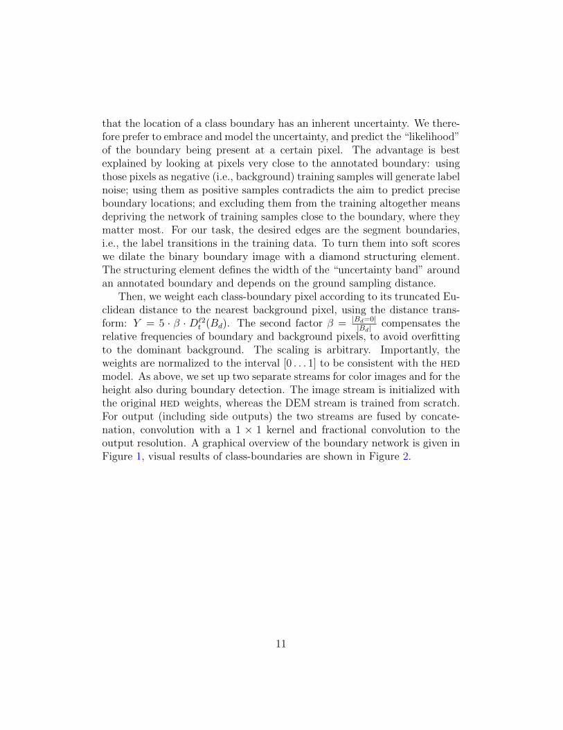
that the location of a class boundary has an inherent uncertainty. We there-fore prefer to embrace and model the uncertainty, and predict the “likelihood”of the boundary being present at a certain pixel. The advantage is bestexplained by looking at pixels very close to the annotated boundary: usingthose pixels as negative (i.e., background) training samples will generate labelnoise; using them as positive samples contradicts the aim to predict preciseboundary locations; and excluding them from the training altogether meansdepriving the network of training samples close to the boundary, where theymatter most. For our task, the desired edges are the segment boundaries,i.e., the label transitions in the training data. To turn them into soft scoreswe dilate the binary boundary image with a diamond structuring element.The structuring element defines the width of the “uncertainty band” aroundan annotated boundary and depends on the ground sampling distance.

Then, we weight each class-boundary pixel according to its truncated Eu-clidean distance to the nearest background pixel, using the distance trans-form: Y = 5 · β · D`2

t (Bd). The second factor β = |Bd=0||Bd|

compensates therelative frequencies of boundary and background pixels, to avoid overfittingto the dominant background. The scaling is arbitrary. Importantly, theweights are normalized to the interval [0 . . . 1] to be consistent with the hedmodel. As above, we set up two separate streams for color images and for theheight also during boundary detection. The image stream is initialized withthe original hed weights, whereas the DEM stream is trained from scratch.For output (including side outputs) the two streams are fused by concate-nation, convolution with a 1 × 1 kernel and fractional convolution to theoutput resolution. A graphical overview of the boundary network is given inFigure 1, visual results of class-boundaries are shown in Figure 2.

11

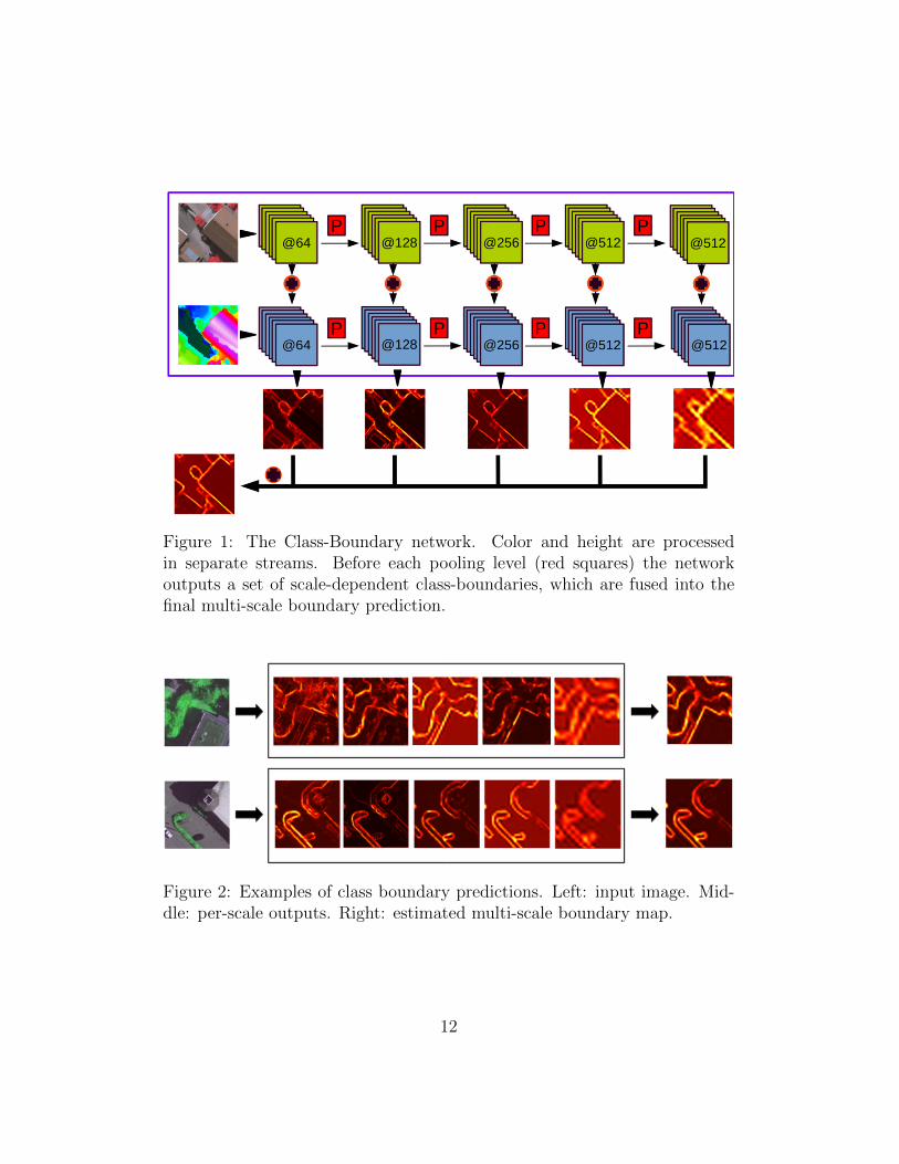
Figure 1: The Class-Boundary network. Color and height are processedin separate streams. Before each pooling level (red squares) the networkoutputs a set of scale-dependent class-boundaries, which are fused into thefinal multi-scale boundary prediction.

Figure 2: Examples of class boundary predictions. Left: input image. Mid-dle: per-scale outputs. Right: estimated multi-scale boundary map.

12

dlr/eth semantic segmentation network

From the literature (Simonyan and Zisserman, 2014) it is known that, alsofor strong classifiers like CNNs, ensemble averaging tends to improve classi-fication results. For highest classification accuracy we thus experiment withan ensemble of multiple CNNs. To that end we use our previous dlr/ethsemantic segmentation network, which has already shown competitive per-formance for remote sensing problems (Marmanis et al., 2016).

Contrary to segnet this model is derived from the standard fcn andhas fully connected layers (reordered into convolutions). It is thus heavierin terms of memory and training, but empirically improves the predictions,presumably because the network can learn extensive high-level, global ob-ject information. Compared to the original fcn (Long et al., 2015), ourvariant has additional skip connections to minimize information loss fromdownsampling. As above, it has separate streams for image and DEM data.

3.2. Integrated class boundary detection and segmentation

Our strategy to combine class boundary detection with semantic segmen-tation is straight-forward: boundary likelihoods are treated as an additional“channel”. In the image stream, the input is the raw colour image; in theDSM stream it is a 2-channel image consisting of the raw DSM and the nDSM(generated by automatically filtering above-ground objects and subtractingthe result from the DSM). In both cases, the input is first passed through thehed network, producing a scalar image of boundary likelihoods. That imageis concatenated to the raw input as an additional channel to form the inputfor the corresponding stream of the semantic segmentation network (note,in CNN language this can be seen as a skip connection that bypasses theboundary detection layers). For segnet, a further skip connection bypassesmost of the segmentation network and reinjects the colour image boundariesas an extra channel after merging the image and DSM streams, before thefinal label prediction. See Figure 3.

13

Figure 3: Semantic segmentation architectures tested in this work. Top: ourmulti-scale segnet architecture. Bottom: our fcn architecture (identicalto our vgg except for initial weights). The boundary detection networkis collapsed (violet box) for better readability. Encoder parts that reducespatial resolution are marked in red, decoder parts that increase resolutionare green. Orange denotes fusion by concatenation, (1× 1) convolution, andupsampling (as required).

The entire processing chain is trained end-to-end (see below for details),using boundaries as supervision signal for the hed layers and segmentationsfor the remaining network.

14

3.3. Ensemble learning

As discussed above, ensemble averaging typically improves DCNN pre-dictions further. We thus also experiment with that strategy and combinethe predictions of three different boundary-aware networks (given the effortto train deep networks, “ensembles” are typically small). In order to addtwo more high-quality models to the ensemble, we have trained two versionsof the dlr/eth network with integrated hed boundary detector, one ini-tialised with the original fcn weights and the other initialised with vgg-16weights.4 In both cases, the DEM channel is again trained from randominitialisations.

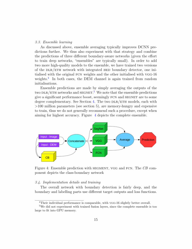
Ensemble predictions are made by simply averaging the outputs of thetwo dlr/eth networks and segnet.5 We note that the ensemble predictionsgive a significant performance boost, seemingly fcn and segnet are to somedegree complementary. See Section 4. The two dlr/eth models, each with>100 million parameters (see section 5), are memory-hungry and expensiveto train, thus we do not generally recommend such a procedure, except whenaiming for highest accuracy. Figure 4 depicts the complete ensemble.

Figure 4: Ensemble prediction with segment, vgg and fcn. The CB com-ponent depicts the class-boundary network

3.4. Implementation details and training

The overall network with boundary detection is fairly deep, and theboundary and labelling parts use different target outputs and loss functions.

4Their individual performance is comparable, with vgg-16 slightly better overall.5We did not experiment with trained fusion layers, since the complete ensemble is too

large to fit into GPU memory.

15

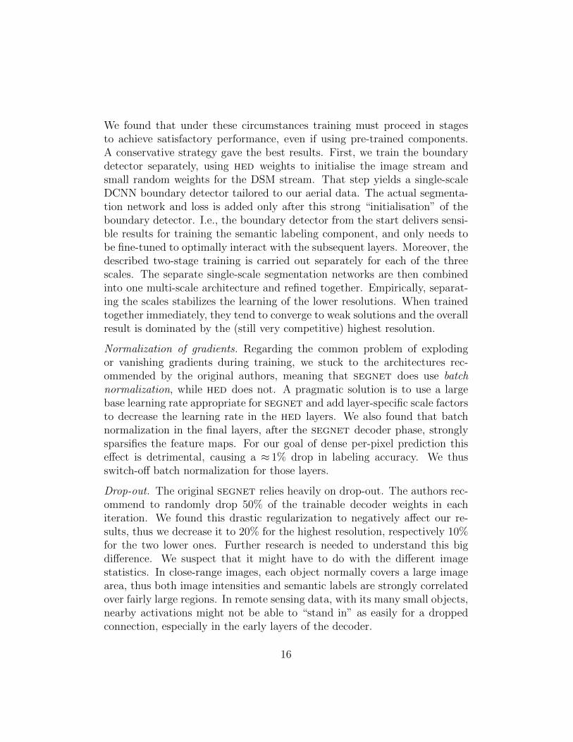
We found that under these circumstances training must proceed in stagesto achieve satisfactory performance, even if using pre-trained components.A conservative strategy gave the best results. First, we train the boundarydetector separately, using hed weights to initialise the image stream andsmall random weights for the DSM stream. That step yields a single-scaleDCNN boundary detector tailored to our aerial data. The actual segmenta-tion network and loss is added only after this strong “initialisation” of theboundary detector. I.e., the boundary detector from the start delivers sensi-ble results for training the semantic labeling component, and only needs tobe fine-tuned to optimally interact with the subsequent layers. Moreover, thedescribed two-stage training is carried out separately for each of the threescales. The separate single-scale segmentation networks are then combinedinto one multi-scale architecture and refined together. Empirically, separat-ing the scales stabilizes the learning of the lower resolutions. When trainedtogether immediately, they tend to converge to weak solutions and the overallresult is dominated by the (still very competitive) highest resolution.

Normalization of gradients. Regarding the common problem of explodingor vanishing gradients during training, we stuck to the architectures rec-ommended by the original authors, meaning that segnet does use batchnormalization, while hed does not. A pragmatic solution is to use a largebase learning rate appropriate for segnet and add layer-specific scale factorsto decrease the learning rate in the hed layers. We also found that batchnormalization in the final layers, after the segnet decoder phase, stronglysparsifies the feature maps. For our goal of dense per-pixel prediction thiseffect is detrimental, causing a ≈ 1% drop in labeling accuracy. We thusswitch-off batch normalization for those layers.

Drop-out. The original segnet relies heavily on drop-out. The authors rec-ommend to randomly drop 50% of the trainable decoder weights in eachiteration. We found this drastic regularization to negatively affect our re-sults, thus we decrease it to 20% for the highest resolution, respectively 10%for the two lower ones. Further research is needed to understand this bigdifference. We suspect that it might have to do with the different imagestatistics. In close-range images, each object normally covers a large imagearea, thus both image intensities and semantic labels are strongly correlatedover fairly large regions. In remote sensing data, with its many small objects,nearby activations might not be able to “stand in” as easily for a droppedconnection, especially in the early layers of the decoder.

16

Data Augmentation. DCNNs need large amounts of training data, which arenot always available. It is standard practice to artificially increase the amountand variation of training data by randomly applying plausible transforma-tions to the inputs. Synthetic data augmentation is particularly relevant forremote sensing data to avoid over-fitting: in a typical mapping project thetraining data comes in the form of a few spatially contiguous regions thathave been annotated, not as individual pixels randomly scattered across theregion of interest. This means that the network is prone to learn local biaseslike the size of houses or the orientation of the road network particular tothe training region. Random transformations – in the example, scaling androtation – will prevent such over-fitting.

In our experiments we used the following transformations for data aug-mentation, randomly sampled per mini-batch of the stochastic gradient de-scent (SGD) optimisation: scaling in the range [1 . . . 1.2], rotation by [0◦ . . . 15◦]degrees, linear shear with [0◦ . . . 8◦], translation by [−5 . . . 5] pixels, and ran-dom vertical as well as horizontal reflection.

4. Experiment Results

4.1. Dataset

We conduct experimental evaluations on the ISPRS Vaihingen 2D seman-tic labeling challenge. This is an open benchmark dataset provided online6. The dataset consists of a color infrared orthophoto, a DSM generated bydense image matching, and manually annotated ground truth labels. Addi-tionally, a nDSM has been released by one of the organizers (Gerke, 2014).It was generated by automatically filtering the DSM to a DTM and subtract-ing the two. Overall, there are 33 tiles of ≈ 2500× 2000 pixels at a GSD of≈ 9cm GSD. 16 tiles are available for training and validation, the remaining17 are withheld by the challenge organizers for testing. We thus remove 4tiles (image numbers 5, 7, 23, 30) from the training set and use them asvalidation set for our experiments. All results refer to that validation set,unless noted otherwise.

6http://www2.isprs.org/commissions/comm3/wg4/2d-sem-label-vaihingen.

html

17

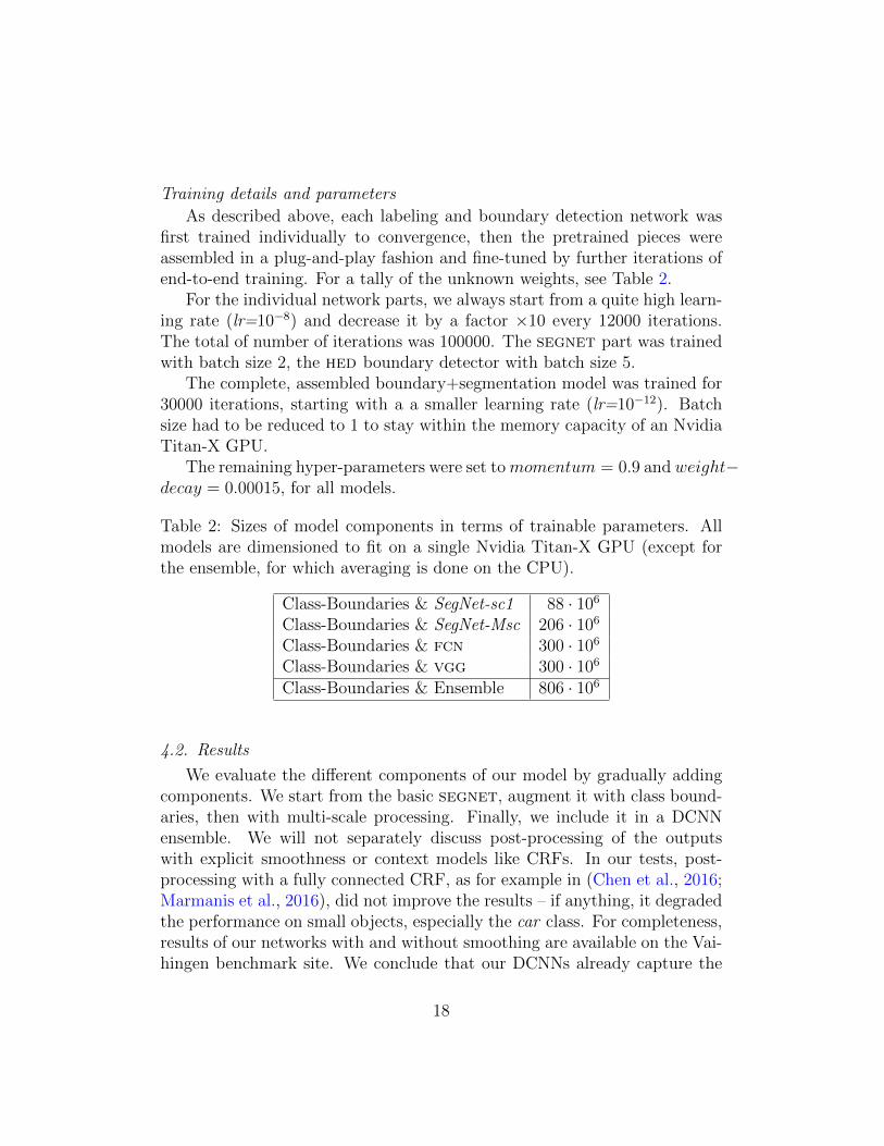
Training details and parameters

As described above, each labeling and boundary detection network wasfirst trained individually to convergence, then the pretrained pieces wereassembled in a plug-and-play fashion and fine-tuned by further iterations ofend-to-end training. For a tally of the unknown weights, see Table 2.

For the individual network parts, we always start from a quite high learn-ing rate (lr=10−8) and decrease it by a factor ×10 every 12000 iterations.The total of number of iterations was 100000. The segnet part was trainedwith batch size 2, the hed boundary detector with batch size 5.

The complete, assembled boundary+segmentation model was trained for30000 iterations, starting with a a smaller learning rate (lr=10−12). Batchsize had to be reduced to 1 to stay within the memory capacity of an NvidiaTitan-X GPU.

The remaining hyper-parameters were set tomomentum = 0.9 and weight−decay = 0.00015, for all models.

Table 2: Sizes of model components in terms of trainable parameters. Allmodels are dimensioned to fit on a single Nvidia Titan-X GPU (except forthe ensemble, for which averaging is done on the CPU).

Class-Boundaries & SegNet-sc1 88 · 106

Class-Boundaries & SegNet-Msc 206 · 106

Class-Boundaries & fcn 300 · 106

Class-Boundaries & vgg 300 · 106

Class-Boundaries & Ensemble 806 · 106

4.2. Results

We evaluate the different components of our model by gradually addingcomponents. We start from the basic segnet, augment it with class bound-aries, then with multi-scale processing. Finally, we include it in a DCNNensemble. We will not separately discuss post-processing of the outputswith explicit smoothness or context models like CRFs. In our tests, post-processing with a fully connected CRF, as for example in (Chen et al., 2016;Marmanis et al., 2016), did not improve the results – if anything, it degradedthe performance on small objects, especially the car class. For completeness,results of our networks with and without smoothing are available on the Vai-hingen benchmark site. We conclude that our DCNNs already capture the

18

context in large context windows. Indeed, this is in our view a main reasonfor their excellent performance.

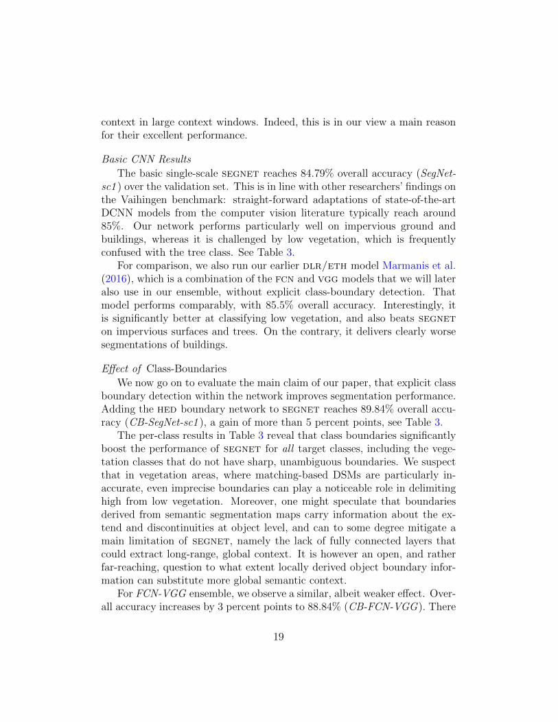
Basic CNN Results

The basic single-scale segnet reaches 84.79% overall accuracy (SegNet-sc1 ) over the validation set. This is in line with other researchers’ findings onthe Vaihingen benchmark: straight-forward adaptations of state-of-the-artDCNN models from the computer vision literature typically reach around85%. Our network performs particularly well on impervious ground andbuildings, whereas it is challenged by low vegetation, which is frequentlyconfused with the tree class. See Table 3.

For comparison, we also run our earlier dlr/eth model Marmanis et al.(2016), which is a combination of the fcn and vgg models that we will lateralso use in our ensemble, without explicit class-boundary detection. Thatmodel performs comparably, with 85.5% overall accuracy. Interestingly, itis significantly better at classifying low vegetation, and also beats segneton impervious surfaces and trees. On the contrary, it delivers clearly worsesegmentations of buildings.

Effect of Class-Boundaries

We now go on to evaluate the main claim of our paper, that explicit classboundary detection within the network improves segmentation performance.Adding the hed boundary network to segnet reaches 89.84% overall accu-racy (CB-SegNet-sc1 ), a gain of more than 5 percent points, see Table 3.

The per-class results in Table 3 reveal that class boundaries significantlyboost the performance of segnet for all target classes, including the vege-tation classes that do not have sharp, unambiguous boundaries. We suspectthat in vegetation areas, where matching-based DSMs are particularly in-accurate, even imprecise boundaries can play a noticeable role in delimitinghigh from low vegetation. Moreover, one might speculate that boundariesderived from semantic segmentation maps carry information about the ex-tend and discontinuities at object level, and can to some degree mitigate amain limitation of segnet, namely the lack of fully connected layers thatcould extract long-range, global context. It is however an open, and ratherfar-reaching, question to what extent locally derived object boundary infor-mation can substitute more global semantic context.

For FCN-VGG ensemble, we observe a similar, albeit weaker effect. Over-all accuracy increases by 3 percent points to 88.84% (CB-FCN-VGG). There

19

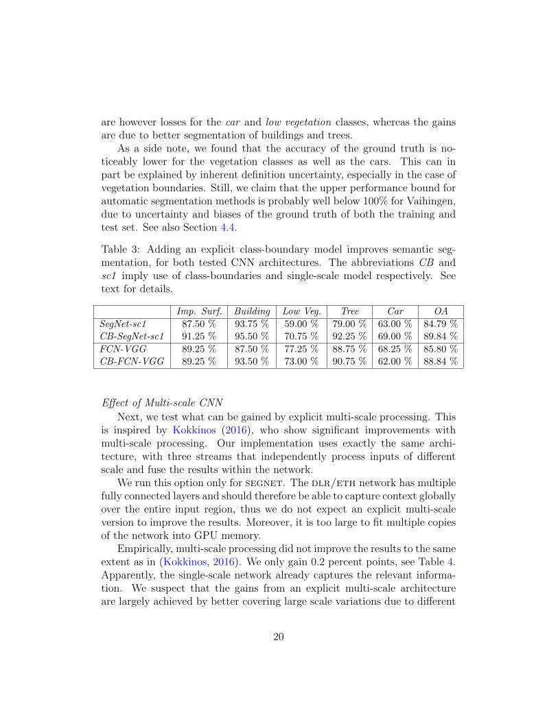
are however losses for the car and low vegetation classes, whereas the gainsare due to better segmentation of buildings and trees.

As a side note, we found that the accuracy of the ground truth is no-ticeably lower for the vegetation classes as well as the cars. This can inpart be explained by inherent definition uncertainty, especially in the case ofvegetation boundaries. Still, we claim that the upper performance bound forautomatic segmentation methods is probably well below 100% for Vaihingen,due to uncertainty and biases of the ground truth of both the training andtest set. See also Section 4.4.

Table 3: Adding an explicit class-boundary model improves semantic seg-mentation, for both tested CNN architectures. The abbreviations CB andsc1 imply use of class-boundaries and single-scale model respectively. Seetext for details.

Imp. Surf. Building Low Veg. Tree Car OA

SegNet-sc1 87.50 % 93.75 % 59.00 % 79.00 % 63.00 % 84.79 %CB-SegNet-sc1 91.25 % 95.50 % 70.75 % 92.25 % 69.00 % 89.84 %

FCN-VGG 89.25 % 87.50 % 77.25 % 88.75 % 68.25 % 85.80 %CB-FCN-VGG 89.25 % 93.50 % 73.00 % 90.75 % 62.00 % 88.84 %

Effect of Multi-scale CNN

Next, we test what can be gained by explicit multi-scale processing. Thisis inspired by Kokkinos (2016), who show significant improvements withmulti-scale processing. Our implementation uses exactly the same archi-tecture, with three streams that independently process inputs of differentscale and fuse the results within the network.

We run this option only for segnet. The dlr/eth network has multiplefully connected layers and should therefore be able to capture context globallyover the entire input region, thus we do not expect an explicit multi-scaleversion to improve the results. Moreover, it is too large to fit multiple copiesof the network into GPU memory.

Empirically, multi-scale processing did not improve the results to the sameextent as in (Kokkinos, 2016). We only gain 0.2 percent points, see Table 4.Apparently, the single-scale network already captures the relevant informa-tion. We suspect that the gains from an explicit multi-scale architectureare largely achieved by better covering large scale variations due to different

20

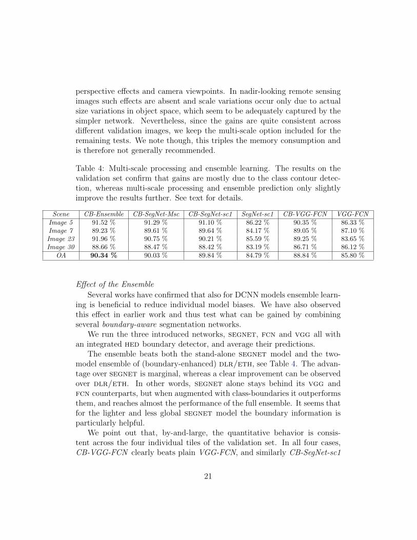
perspective effects and camera viewpoints. In nadir-looking remote sensingimages such effects are absent and scale variations occur only due to actualsize variations in object space, which seem to be adequately captured by thesimpler network. Nevertheless, since the gains are quite consistent acrossdifferent validation images, we keep the multi-scale option included for theremaining tests. We note though, this triples the memory consumption andis therefore not generally recommended.

Table 4: Multi-scale processing and ensemble learning. The results on thevalidation set confirm that gains are mostly due to the class contour detec-tion, whereas multi-scale processing and ensemble prediction only slightlyimprove the results further. See text for details.

Scene CB-Ensemble CB-SegNet-Msc CB-SegNet-sc1 SegNet-sc1 CB-VGG-FCN VGG-FCNImage 5 91.52 % 91.29 % 91.10 % 86.22 % 90.35 % 86.33 %Image 7 89.23 % 89.61 % 89.64 % 84.17 % 89.05 % 87.10 %Image 23 91.96 % 90.75 % 90.21 % 85.59 % 89.25 % 83.65 %Image 30 88.66 % 88.47 % 88.42 % 83.19 % 86.71 % 86.12 %

OA 90.34 % 90.03 % 89.84 % 84.79 % 88.84 % 85.80 %

Effect of the Ensemble

Several works have confirmed that also for DCNN models ensemble learn-ing is beneficial to reduce individual model biases. We have also observedthis effect in earlier work and thus test what can be gained by combiningseveral boundary-aware segmentation networks.

We run the three introduced networks, segnet, fcn and vgg all withan integrated hed boundary detector, and average their predictions.

The ensemble beats both the stand-alone segnet model and the two-model ensemble of (boundary-enhanced) dlr/eth, see Table 4. The advan-tage over segnet is marginal, whereas a clear improvement can be observedover dlr/eth. In other words, segnet alone stays behind its vgg andfcn counterparts, but when augmented with class-boundaries it outperformsthem, and reaches almost the performance of the full ensemble. It seems thatfor the lighter and less global segnet model the boundary information isparticularly helpful.

We point out that, by-and-large, the quantitative behavior is consis-tent across the four individual tiles of the validation set. In all four cases,CB-VGG-FCN clearly beats plain VGG-FCN, and similarly CB-SegNet-sc1

21

comprehensively beats SegNet-sc1. Regarding multi-scale processing, CB-SegNet-Msc wins over CB-SegNet-sc1 except for one case (image 7), wherethe difference are a barely noticeable 0.03 percent points (ca. 1500 pixels /12 m2). Ensemble averaging again help for the other three test tiles, withan average gain of 0.21 percent points, while for image 7 the ensemble pre-diction is better than CB-VGG-FCN but does not quite reach the segnetperformance. A further analysis of the results is left for future work, but willprobably require a larger test set.

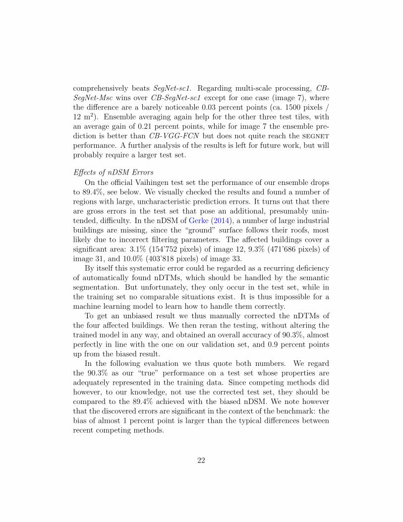
Effects of nDSM Errors

On the official Vaihingen test set the performance of our ensemble dropsto 89.4%, see below. We visually checked the results and found a number ofregions with large, uncharacteristic prediction errors. It turns out that thereare gross errors in the test set that pose an additional, presumably unin-tended, difficulty. In the nDSM of Gerke (2014), a number of large industrialbuildings are missing, since the “ground” surface follows their roofs, mostlikely due to incorrect filtering parameters. The affected buildings cover asignificant area: 3.1% (154’752 pixels) of image 12, 9.3% (471’686 pixels) ofimage 31, and 10.0% (403’818 pixels) of image 33.

By itself this systematic error could be regarded as a recurring deficiencyof automatically found nDTMs, which should be handled by the semanticsegmentation. But unfortunately, they only occur in the test set, while inthe training set no comparable situations exist. It is thus impossible for amachine learning model to learn how to handle them correctly.

To get an unbiased result we thus manually corrected the nDTMs ofthe four affected buildings. We then reran the testing, without altering thetrained model in any way, and obtained an overall accuracy of 90.3%, almostperfectly in line with the one on our validation set, and 0.9 percent pointsup from the biased result.

In the following evaluation we thus quote both numbers. We regardthe 90.3% as our “true” performance on a test set whose properties areadequately represented in the training data. Since competing methods didhowever, to our knowledge, not use the corrected test set, they should becompared to the 89.4% achieved with the biased nDSM. We note howeverthat the discovered errors are significant in the context of the benchmark: thebias of almost 1 percent point is larger than the typical differences betweenrecent competing methods.

22

4.3. Comparison to State-of-the-art

Our proposed class-contour ensemble model is among the top performerson the official benchmark test set, reaching 89.4% overall accuracy, respec-tively 90.3% with the correct nDSM. The strongest competitors are INRIA(89.5%, Maggiori et al., 2016), using a variant of fcn, and ONERA (89.8%,Audebert et al., 2016), with a variant of segnet. Importantly, we achieveabove 90% accuracy over man-made classes, which are the most well-definedones, where accurate segmentation boundaries matter most, see Table 5.

Detailed, results over the performance of the top-ranking models overthe ISPRS benchmark are given in Table 6. Overall, the performance ofdifferent models is very similar, which may not be all that surprising, sincethe top performers are in fact all variants of fcn or segnet . We note ourmodel and INRIA are the most “puristic” ones, in that they do not use anyhand-engineered image features. ONERA uses the NDVI as additional inputchannel; DST seemingly includes a random forest in its ensemble, whoseinput features include the NDVI (Normalized Vegetation Index) as well asstatistics over the DSM normals. It appears that the additional featuresenable a similar performance boost as our class boundaries, although it is atthis point unclear whether they encode the same information. Interestingly,our model scores rather well on the car class, although we do not use anystratified sampling to boost rare classes. We believe that this is in part aconsequence of not smoothing the label probabilities.

One can also see that after correcting the nDSM for large errors, ourperformance is 0.9 percent point above the closest competitor for impervioussurfaces, while it is also 0.5 percent ahead for buildings. The bias in thetest data thus seems to affect all models. Somewhat surprisingly, our scoreson the vegetation classes are also on par with the competitors, althoughintuitively contours cannot contribute as much for those classes, becausetheir boundaries are not well-defined. Still, they significantly improve thesegmentation of vegetation classes, c.f. 3. Empirically, the multi-scale class-boundaries information boosts segmentation of the tree and low vegetationclasses to a level reached by models that use a dedicated NDVI channel. Acloser look at the underlying mechanisms is left for future work.

4.4. A word on data quality

In our experiments, we repeatedly noticed inaccuracies of the groundtruth data (similar observations were made by Paisitkriangkrai et al. (2015)).Obviously, a certain degree of uncertainty is unavoidable when annotating

23

Table 5: Confusion matrix of our best result on the private Vaihingen testset.

Impervious Building Low-Vegetation Tree Car

Impervious 93.2 % 2.2 % 3.6 % 0.9 % 0.1 %

Building 2.8 % 95.3 % 1.6 % 0.3 % 0.0 %

Low-Vegetation 3.7 % 1.4 % 82.5 % 12.5 % 0.0 %

Tree 0.7 % 0.2 % 6.9 % 92.3% 0.0 %

Car 19.5 % 7.0 % 0.5 % 0.4 % 72.60 %

Precision 91.6 % 95.0 % 85.5 % 87.5 % 92.1 %

Recall 93.2 % 95.3 % 82.5 % 92.3% 72.6 %

F1-score 92.4 % 95.2 % 83.9 % 89.9 % 81.2 %

Table 6: Per-class F1-scores and overall accuracies of top performers on theVaihingen benchmark (numbers copied from benchmark website). DLR 7 isour ensemble model, DLR 9 is our ensemble with corrected nDSM.

Impervious Building Low-Vegetation Tree Car OA

DST 2 90.5 % 93.7 % 83.4 % 89.2 % 72.6 % 89.1 %

INR 91.1 % 94.7 % 83.4 % 89.3 % 71.2 % 89.5 %

ONE 6 91.5 % 94.3 % 82.7 % 89.3 % 85.7 % 89.4 %

ONE 7 91.0 % 94.5 % 84.4 % 89.9 % 77.8 % 89.8 %

DLR 7 91.4 % 93.8 % 83.0 % 89.3 % 82.1 % 89.4 %

DLR 9 92.4 % 95.2 % 83.9 % 89.9 % 81.2 % 90.3 %

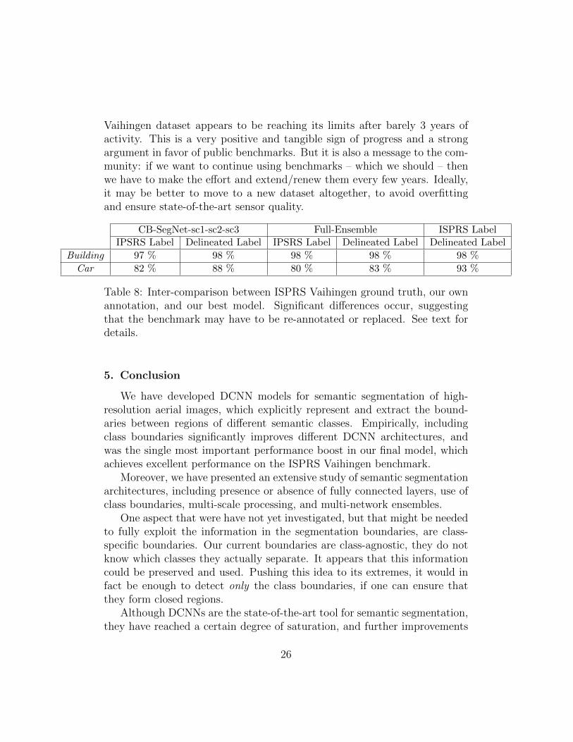
data, in particular in remote sensing images with their small objects andmany boundaries. We thus decided to re-annotate one image (image-23 )from our validation set with great care, to assess the “inherent” labelingaccuracy. We did this only for the two easiest classes buildings and cars, sincethe remaining classes have significant definition uncertainty and we could notensure to use exactly the same definitions as the original annotators.

We then evaluate the new annotation, the ground truth from the bench-mark, and the output of our best model, against each other. Results areshown in Table 8. One can see significant differences, especially for the carswhich are small and have a large fraction of pixels near the boundary. Consid-ering the saturating progress on the benchmark – differences between recentsubmissions are generally < 2% – there is a very real danger that annotationerrors influence the results and conclusions. It may be surprising, but the

24

Image FCN-VGG CB-SegNet CB-Ensemble

Table 7: Visual examples of predictions on the official ISPRS tes-set. The re-sults of FCN-VGG, CB-SegNet, CB-Ensemble associate to our online officialsubmissions, namely DLR 1, DLR 5 and DLR 7 respectively. Legend-colors,White: Impervious Surfaces, Blue: Buildings, Cyan: Low-Vegetation,Green: Trees, Yellow: Cars

Vaihingen dataset appears to be reaching its limits after barely 3 years ofactivity. This is a very positive and tangible sign of progress and a strongargument in favor of public benchmarks. But it is also a message to the com-munity: if we want to continue using benchmarks – which we should – thenwe have to make the effort and extend/renew them every few years. Ideally,it may be better to move to a new dataset altogether, to avoid overfittingand ensure state-of-the-art sensor quality.

CB-SegNet-sc1-sc2-sc3 Full-Ensemble ISPRS LabelIPSRS Label Delineated Label IPSRS Label Delineated Label Delineated Label

Building 97 % 98 % 98 % 98 % 98 %

Car 82 % 88 % 80 % 83 % 93 %

Table 8: Inter-comparison between ISPRS Vaihingen ground truth, our ownannotation, and our best model. Significant differences occur, suggestingthat the benchmark may have to be re-annotated or replaced. See text fordetails.

5. Conclusion

We have developed DCNN models for semantic segmentation of high-resolution aerial images, which explicitly represent and extract the bound-aries between regions of different semantic classes. Empirically, includingclass boundaries significantly improves different DCNN architectures, andwas the single most important performance boost in our final model, whichachieves excellent performance on the ISPRS Vaihingen benchmark.

Moreover, we have presented an extensive study of semantic segmentationarchitectures, including presence or absence of fully connected layers, use ofclass boundaries, multi-scale processing, and multi-network ensembles.

One aspect that were have not yet investigated, but that might be neededto fully exploit the information in the segmentation boundaries, are class-specific boundaries. Our current boundaries are class-agnostic, they do notknow which classes they actually separate. It appears that this informationcould be preserved and used. Pushing this idea to its extremes, it would infact be enough to detect only the class boundaries, if one can ensure thatthey form closed regions.

Although DCNNs are the state-of-the-art tool for semantic segmentation,they have reached a certain degree of saturation, and further improvements

26

of segmentation quality will probably be small, tedious, and increasinglyproblem-specific. Nevertheless, there are several promising directions forfuture research. We feel that model size is becoming an issue. Given theexcessive size and complexity of all the best-performing DCNN models, aninteresting option would be to develop methods for compressing large, deepmodels into smaller, more compact ones for further processing. First ideasin this direction have been brought up by Hinton et al. (2015).

References

References

Audebert, N., Saux, B. L., Lefevre, S., 2016. Semantic segmentation of earthobservation data using multimodal and multi-scale deep networks. arXivpreprint arXiv:1609.06846.

Badrinarayanan, V., Kendall, A., Cipolla, R., 2015. Segnet: A deep convolu-tional encoder-decoder architecture for image segmentation. arXiv preprintarXiv:1511.00561.

Barnsley, M. J., Barr, S. L., 1996. Inferring urban land use from satellitesensor images using kernel-based spatial reclassification. PhotogrammetrivEngineering and Remote Sensing 62 (8), 949–958.

Bertasius, G., Shi, J., Torresani, L., 2015. High-for-low and low-for-high:Efficient boundary detection from deep object features and its applicationsto high-level vision. In: Proceedings of the IEEE International Conferenceon Computer Vision. pp. 504–512.

Bischof, H., Schneider, W., Pinz, A. J., 1992. Multispectral classification oflandsat-images using neural networks. IEEE Transactions on Geoscienceand Remote Sensing 30 (3), 482–490.

Chen, L.-C., Barron, J. T., Papandreou, G., Murphy, K., Yuille, A. L.,2015. Semantic image segmentation with task-specific edge detection us-ing cnns and a discriminatively trained domain transform. arXiv preprintarXiv:1511.03328.

Chen, L.-C., Papandreou, G., Kokkinos, I., Murphy, K., Yuille, A. L., 2014.Semantic image segmentation with deep convolutional nets and fully con-nected crfs. arXiv preprint arXiv:1412.7062.

27

Chen, L.-C., Papandreou, G., Kokkinos, I., Murphy, K., Yuille, A. L., 2016.DeepLab: Semantic image segmentation with deep convolutional nets,atrous convolution, and fully connected CRFs. CoRR abs/1606.00915.URL http://arxiv.org/abs/1606.00915

Dai, J., He, K., Sun, J., 2015. Instance-aware semantic segmentation viamulti-task network cascades. arXiv preprint arXiv:1512.04412.

Dalla Mura, M., Benediktsson, J. A., Waske, B., Bruzzone, L., 2010. Mor-phological attribute profiles for the analysis of very high resolution images.IEEE Transactions on Geoscience and Remote Sensing 48 (10), 3747–3762.

Dosovitskiy, A., Fischer, P., Ilg, E., Hausser, P., Hazırbas, C., Golkov, V.,v.d. Smagt, P., Cremers, D., Brox, T., 2015. FlowNet: Learning opticalflow with convolutional networks. In: IEEE International Conference onComputer Vision (ICCV).

Farabet, C., Couprie, C., Najman, L., LeCun, Y., 2013. Learning hierarchi-cal features for scene labeling. IEEE transactions on pattern analysis andmachine intelligence 35 (8), 1915–1929.

Franklin, S. E., McDermid, G. J., 1993. Empirical relations between digitalSPOT HRV and CASI spectral resonse and lodgepole pine (pinus contorta)forest stand parameters. International Journal of Remote Sensing 14 (12),2331–2348.

Fu, K. S., Landgrebe, D. A., Phillips, T. L., 1969. Information processing ofremotely sensed agricultural data. Proceedings of the IEEE 57 (4), 639–653.

Gal, Y., Ghahramani, Z., 2015. Dropout as a bayesian approxima-tion: Representing model uncertainty in deep learning. arXiv preprintarXiv:1506.02142.

Gerke, M., 2014. Use of the stair vision library within the isprs 2d semanticlabeling benchmark (vaihingen). Tech. rep., ITC, University of Twente.

Grangier, D., Bottou, L., Collobert, R., 2009. Deep convolutional networksfor scene parsing. In: ICML 2009 Deep Learning Workshop. Vol. 3. Cite-seer.

28

Hinton, G., Vinyals, O., Dean, J., 2015. Distilling the knowledge in a neuralnetwork. arXiv preprint arXiv:1503.02531.

Kampffmeyer, M., Salberg, A.-B., Jenssen, R., 2016. Semantic segmentationof small objects and modeling of uncertainty in urban remote sensing im-ages using deep convolutional neural networks. In: Proceedings of the IEEEConference on Computer Vision and Pattern Recognition Workshops. pp.1–9.

Kokkinos, I., 2016. Pushing the boundaries of boundary detection usingdeep learning. In: International Conference on Learning Representations(ICLR).

Krahenbuhl, P., Koltun, V., 2011. Efficient inference in fully connected crfswith gaussian edge potentials. In: Advances in Neural Information Pro-cessing Systems.

Langkvist, M., Kiselev, A., Alirezaie, M., Loutfi, A., 2016. Classificationand segmentation of satellite orthoimagery using convolutional neural net-works. Remote Sensing 8 (4), 329.

Lee, C.-Y., Xie, S., Gallagher, P., Zhang, Z., Tu, Z., 2015. Deeply-supervisednets. In: AISTATS.

Long, J., Shelhamer, E., Darrell, T., 2015. Fully convolutional networks forsemantic segmentation. In: Proceedings of the IEEE Conference on Com-puter Vision and Pattern Recognition. pp. 3431–3440.

Maggiori, E., Tarabalka, Y., Charpiat, G., Alliez, P., 2016. High-resolutionsemantic labeling with convolutional neural networks. arXiv preprintarXiv:1611.01962.

Malmgren-Hansen, D., Nobel-J, M., et al., 2015. Convolutional neural net-works for sar image segmentation. In: 2015 IEEE International Sympo-sium on Signal Processing and Information Technology (ISSPIT). IEEE,pp. 231–236.

Marcu, A., Leordeanu, M., 2016. Dual local-global contextual pathways forrecognition in aerial imagery. arXiv preprint arXiv:1605.05462.

29

Marmanis, D., Wegner, J., Galliani, S., Schindler, K., Datcu, M., Stilla, U.,2016. Semantic segmentation of aerial images with an ensemble of cnns. IS-PRS Annals of Photogrammetry, Remote Sensing and Spatial InformationSciences, 473–480.

Mayer, H., Hinz, S., Bacher, U., Baltsavias, E., 2006. A test of automaticroad extraction approaches. ISPRS Annals 36 (3), 209–214.

Mnih, V., Hinton, G. E., 2010. Learning to detect roads in high-resolutionaerial images. In: European Conference on Computer Vision. Springer, pp.210–223.

Mou, L., Zhu, X., 2016. Spatiotemporal scene interpretation of space videosvia deep neural network and tracklet analysis. In: 2016 IEEE InternationalGeoscience and Remote Sensing Symposium (IGARSS). IEEE, pp. 4959–4962.

Noh, H., Hong, S., Han, B., 2015. Learning deconvolution network for seman-tic segmentation. In: Proceedings of the IEEE International Conference onComputer Vision. pp. 1520–1528.

Paisitkriangkrai, S., Sherrah, J., Janney, P., Hengel, V.-D., et al., 2015. Effec-tive semantic pixel labelling with convolutional networks and conditionalrandom fields. In: Proceedings of the IEEE Conference on Computer Vi-sion and Pattern Recognition Workshops. pp. 36–43.

Pinheiro, P. H., Collobert, R., 2014. Recurrent convolutional neural networksfor scene labeling. In: ICML. pp. 82–90.

Pinheiro, P. O., Lin, T.-Y., Collobert, R., Dollar, P., 2016. Learning to refineobject segments. arXiv preprint arXiv:1603.08695.

Richards, J. A., 2013. Remote sensing digital image analysis. Springer.

Saito, S., Yamashita, T., Aoki, Y., 2016. Multiple object extraction fromaerial imagery with convolutional neural networks. Electronic Imaging2016 (10), 1–9.

Sherrah, J., 2016. Fully convolutional networks for dense semantic labellingof high-resolution aerial imagery. arXiv preprint arXiv:1606.02585.

30

Simonyan, K., Zisserman, A., 2014. Very deep convolutional networks forlarge-scale image recognition. arXiv preprint arXiv:1409.1556.

Socher, R., Huval, B., Bhat, B., Manning, C. D., Ng, A. Y., 2012.Convolutional-recursive deep learning for 3d object classification. In: Ad-vances in Neural Information Processing Systems 25.

Szeliski, R., 2010. Computer vision: algorithms and applications. Springer.

Tokarczyk, P., Wegner, J. D., Walk, S., Schindler, K., 2015. Features, colorspaces, and boosting: New insights on semantic classification of remotesensing images. IEEE Transactions on Geoscience and Remote Sensing53 (1), 280–295.

Volpi, M., Tuia, D., 2016. Dense semantic labeling of sub-decimeterresolution images with convolutional neural networks. arXiv preprintarXiv:1608.00775.

Xie, S., Tu, Z., 2015. Holistically-nested edge detection. In: Proceedings ofthe IEEE International Conference on Computer Vision. pp. 1395–1403.

Yang, J., Price, B., Cohen, S., Lee, H., Yang, M.-H., 2016. Object contour de-tection with a fully convolutional encoder-decoder network. arXiv preprintarXiv:1603.04530.

Yu, F., Koltun, V., 2016. Multi-scale context aggregation by dilated convolu-tions. In: International Conference on Learning Representations (ICLR).

Zeiler, M. D., Fergus, R., 2014. Visualizing and understanding convolutionalnetworks. In: European Conference on Computer Vision. Springer, pp.818–833.

31