classification of varieties with canonical curve...
TRANSCRIPT

CLASSIFICATION OF VARIETIES WITH CANONICAL CURVE SECTION
VIA GAUSSIAN MAPS ON CANONICAL CURVES
CIRO CILIBERTO*, ANGELO FELICE LOPEZ* AND RICK MIRANDA**
The purpose of this article is to further develop a method to classifyvarieties X ⊂ IPN having canonical curve section, using Gaussian mapcomputations. In a previous article we applied these techniques to clas-sify prime Fano threefolds, that is Fano threefolds whose Picard groupis generated by the hyperplane bundle. In this article we extend thismethod and classify Fano threefolds of higher index and Mukai varieties,i.e. varieties of dimension four or more with canonical curve sections.First we determine when the Hilbert scheme H of such varieties X is nonempty. Moreover, in the case of Picard number one, we prove that H isirreducible and that the examples of Fano-Iskovskih and Mukai form adense open subset of smooth points of H.
1. INTRODUCTION
Let C ⊂ IP g−1 be a smooth canonical curve of genus g ≥ 3. The purpose of this
article is to further develop a method to classify varieties having C as their curve section,
following the techniques of [CLM1]. In that article a careful analysis of the degeneration
to the cone over the hyperplane section was made for prime Fano threefolds, that is Fano
threefolds whose Picard group is generated by the hyperplane bundle. In this article we
1991 Mathematics Subject Classification: Primary 14J45. Secondary 14J28, 14H10.* Research partially supported by the MURST national project “Geometria Algebrica”;
the authors are members of GNSAGA of CNR.* * Research partially supported by NSF under grant DMS-9104058.

CILIBERTO-LOPEZ-MIRANDA 2
extend this method and classify Fano threefolds of higher index (which still have Picard
number one) (see Theorem (3.2)). We are also able to classify Mukai varieties, i.e. varieties
of dimension four or more with canonical curve sections (see Theorem (3.15)).
The classification of the varieties in question has been executed before, mostly by
Fano, with modern proofs given by Iskovskih, Mukai and others. These proofs rely on
several deep theorems, in particular for the Fano threefolds, the existence of lines and of
smooth sections in the primitive submultiple of the anticanonical line bundle.
Our approach to the classification is completely different. It is based on a general
remark concerning the degeneration to the cone over the hyperplane section, as mentioned
above. Let V ⊂ IP r be a smooth, irreducible, projectively Cohen-Macaulay variety, with
general hyperplane section W . Note that V flatly degenerates to the cone X over W , and
therefore [X] is a point in the Hilbert scheme H of V . Suppose one has an upper bound
for h0(X,NX), which is the dimension of the Zariski tangent space to H at [X]. Suppose
in addition that one has a known irreducible family F of varieties containing [V ] as a
member, and that the dimension of F is equal to the upper bound for h0(X,NX). Since
the closure of F in the Hilbert scheme H must contain the point [X], we conclude that
the dimension of H at [X] is equal to the dimension of its Zariski tangent space there, and
hence [X] is a smooth point of H, and the closure of the known family F is the unique
component of H containing [X] (and [V ]).
One more ingredient now comes into play. Suppose further that the Hilbert scheme
H′ of the hyperplane sections W of V is irreducible, and that one can prove that as V
varies in any component of its Hilbert scheme, the possible hyperplane sections W vary
to fill up H′. This assumption allows us to conclude then that the Hilbert scheme H is
also irreducible: if there were two components, each would contain varieties with general
hyperplane section W , and therefore each would contain the cone point [X] over a general
W . This would force [X] to be a singular point of the Hilbert scheme, which, given the
first part of the argument as described above, is a contradiction. One concludes then that
there is only one component of H, which is the closure of the known family F as described
above. In this sense one obtains a classification result for varieties V .
This scheme can be applied to classify Fano threefolds of the principal series with

CLASSIFICATION OF VARIETIES WITH CANONICAL CURVE SECTION 3
Picard number one. First of all from papers of Fano and Iskovskih one may easily extract
lists of families of such threefolds, and the number of parameters on which they depend
are easily available. (We stress that our classification argument does not rely on the
classification theorems of Fano and Iskovskih, but simply on the existence of the families,
taken as examples.) Secondly an easy deformation theoretic argument proves that the
general hyperplane section of a general Fano threefold of the principal series (and with
Picard number one) varying in any component of the Hilbert scheme, is a general K3
surface of the correct genus. Therefore to complete the program outlined above, we must
give the sharp upper bound for h0(X,NX). By now it is well known that this computation
rests on the study of Gaussian maps for the general curve section C. This is done in section
2 (see Theorem (2.15)).
We are also able to execute the program in an iterative fashion, to obtain similar
classification statements for the Mukai varieties. The list of examples is also available,
together with the number of parameters on which they depend.
The reader will notice that the above scheme provides a classification statement only
when there are actually examples of such varieties. To finish one has to prove a negative
statement, that varieties do not exist when there are no examples. This is provided by a
theorem of Zak and L’vovskii, which, under suitable conditions on the Gaussian map of a
curve, says that this curve cannot be the curve section of a variety which is not a cone.
The Gaussian map computations which we have to perform to prove the classification part,
suffice also to demonstrate the required non existence statement for the Fano and Mukai
varieties.
In section 2 we will recall the definition of the relevant Gaussian maps and we will
perform the computations of the coranks of these maps which are necessary for our pur-
poses, as indicated above. In section 3 we execute the classification program for the Fano
threefolds and Mukai varieties. Since the case of prime Fano threefolds was already treated
in [CLM1], we treat here only the cases of higher index.

CILIBERTO-LOPEZ-MIRANDA 4
2. THE CORANK THEOREM
We recall here the definition of the Gaussian map
ΦωC:∧2
H0(C,ωC)→ H0(C,ω⊗3C )
which sends s∧ t to s⊗ dt− t⊗ ds. The Corank One Theorem from [CLM1] (Theorem 4)
states that for a general hyperplane section Cg of a general prime K3 surface Sg (that is
one whose Picard group is generated by the hyperplane bundle) the corank of the Gaussian
map ΦωCgis one if g = 11 or g ≥ 13.
In this section we will extend this result to reembedded K3 surfaces. Let Hg be the
component of the Hilbert scheme of prime K3 surfaces of genus g ≥ 3. LetH2 be the family
of prime genus 2 K3 surfaces, that is double covers of IP 2 ramified along a sextic curve.
For r ≥ 2 let Hr,g be the component of the Hilbert scheme whose general elements are
obtained by embedding prime K3 surfaces of genus g via the r-th multiple of the primitive
class, except for r = g = 2 when we set H2,2 = H2. Moreover set H1,g = Hg. We denote
by Sr,g any smooth surface represented by a point in Hr,g; note that, for (r, g) 6= (2, 2),
Sr,g = vr(Sg) ⊂ IPN(r,g), where N(r, g) = 1 + r2(g − 1), Sg ⊂ IP g is a K3 surface and vr
is the r-th Veronese embedding. Let Cg be a general hyperplane section of Sg; we will say
that Sr,g is non trigonal (respectively that CliffSr,g ≥ 2 / non DP) if Cg is not a trigonal
curve (respectively CliffCg ≥ 2 / Cg does not lie on a smooth Del Pezzo surface). We
finally denote by Cr,g any smooth curve section of Sr,g, if (r, g) 6= (2, 2), and by C2,2 any
smooth curve in the linear system on S2,2 given by twice the primitive linear system.
The following general remark is the basis of our computation. Let C be a smooth
hyperplane section of a smooth K3 surface S and consider the commutative diagram
(2.1)
∧2H0(S,OS(1))
ΦOS(1)−→ H0(S,Ω1S(2))
↓ φ↓ π H0(C,Ω1
S(2)|C)↓ ψ∧2
H0(C,OC(1))ΦωC−→ H0(C,ω⊗3
C )
where π and φ are restriction maps, ΦOS(1) and ΦωCare Gaussian maps and ψ is the map
on differentials induced by the sheaf map Ω1S |C → Ω1
C . We have the following:

CLASSIFICATION OF VARIETIES WITH CANONICAL CURVE SECTION 5
Lemma (2.2). Let C be a smooth hyperplane section of a smooth K3 surface S, φ
and ψ as in diagram (2.1). If ΦOS(1) and φ are surjective then ΦωChas corank one.
Proof: From (2.1) we have Im ψ = Im (ψ φ ΦOS(1)) = Im (ΦωC π) = Im ΦωC
since
φ ΦOS(1) and π are surjective. On the other hand the exact sequence
0→ N∗C/S(2)→ Ω1S(2)|C → ω⊗3
C → 0
shows that corank ψ ≤ h1(N∗C/S(2)) = h1(OC(1)) = h1(ωC) = 1, hence corank ΦωC= 1
since ΦωCis not surjective by Wahl’s theorem ([W]) because C lies on a K3 surface.
By (2.1) and Lemma (2.2) the computation of the corank of the Gaussian map
ΦωCr,gis then reduced to studying the maps ΦOSr,g (1) and φr,g : H0(Sr,g,Ω
1Sr,g
(2)) →
H0(Cr,g,Ω1Sr,g
(2)|Cr,g). The corank of ΦOSr,g (1) was calculated in [CLM2, Theorem 1.1].
As for φr,g we have:
Lemma (2.3). Suppose k ≥ 1 and r, g are such that either r = 1, g = 11 or g ≥ 13;
or r ≥ 2, g ≥ 2. Then H1(Sr,g,Ω1Sr,g
(k)) = 0 and therefore φr,g,k : H0(Sr,g,Ω1Sr,g
(k+1))→
H0(Cr,g,Ω1Sr,g
(k + 1)|Cr,g) is surjective if one of the following holds:
(a) k ≥ 2 and r ≥ 2, g ≥ 3 except k = r = 2, g = 3;
(b) k = 1 and r = 3, g ≥ 5 or r = 4, g ≥ 4 or r ≥ 5, g ≥ 3;
(c) Sr,g represents a general point of Hr,g, k = 1 and r = 1, g = 11, g ≥ 13 or
r = 2, g ≥ 7;
(d) Sr,2 has smooth ramification divisor, g = 2, k = 1 and r ≥ 4 or k ≥ 2 and r ≥ 3.
Moreover for k = r = 2, g = 3 or k = 1 and r = 4, g = 3 or r = 2, g = 6 and CliffS2,6 ≥ 2,
we have instead corank φr,g,k = 1.
Proof: By definition of Sr,g we have
(2.4) H1(Sr,g,Ω1Sr,g
(k)) ∼= H1(Sg,Ω1Sg
(rk)) ∼= H1(Sg, TSg(−rk))∗
where Sg is a smooth K3 surface representing a point of Hg.
Consider now for g ≥ 3 the Euler sequence of Sg ⊂ IP g tensored by OSg (−j)
(2.5) 0→ OSg(−j)→ H0(OSg
(1))∗ ⊗OSg(1− j)→ TIP g |Sg
(−j)→ 0.
CILIBERTO-LOPEZ-MIRANDA 6
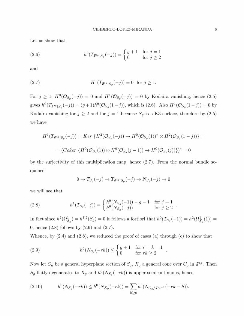
Let us show that
(2.6) h0(TIP g |Sg(−j)) =
g + 1 for j = 10 for j ≥ 2
and
(2.7) H1(TIP g |Sg(−j)) = 0 for j ≥ 1.
For j ≥ 1, H0(OSg (−j)) = 0 and H1(OSg (−j)) = 0 by Kodaira vanishing, hence (2.5)
gives h0(TIP g |Sg(−j)) = (g+ 1)h0(OSg (1− j)), which is (2.6). Also H1(OSg (1− j)) = 0 by
Kodaira vanishing for j ≥ 2 and for j = 1 because Sg is a K3 surface, therefore by (2.5)
we have
H1(TIP g |Sg(−j)) = Ker H2(OSg
(−j))→ H0(OSg(1))∗ ⊗H2(OSg
(1− j)) =
= (Coker H0(OSg (1))⊗H0(OSg (j − 1))→ H0(OSg (j)))∗ = 0
by the surjectivity of this multiplication map, hence (2.7). From the normal bundle se-
quence
0→ TSg(−j)→ TIP g |Sg
(−j)→ NSg(−j)→ 0
we will see that
(2.8) h1(TSg(−j)) =
h0(NSg (−1))− g − 1 for j = 1h0(NSg
(−j)) for j ≥ 2.
In fact since h2(Ω1Sg
) = h1,2(Sg) = 0 it follows a fortiori that h0(TSg(−1)) = h2(Ω1
Sg(1)) =
0, hence (2.8) follows by (2.6) and (2.7).
Whence, by (2.4) and (2.8), we reduced the proof of cases (a) through (c) to show that
(2.9) h0(NSg(−rk)) ≤
g + 1 for r = k = 10 for rk ≥ 2
.
Now let Cg be a general hyperplane section of Sg, Xg a general cone over Cg in IP g. Then
Sg flatly degenerates to Xg and h0(NSg(−rk)) is upper semicontinuous, hence
(2.10) h0(NSg (−rk)) ≤ h0(NXg (−rk)) =∑h≥0
h0(NCg/IP g−1(−rk − h)).

CLASSIFICATION OF VARIETIES WITH CANONICAL CURVE SECTION 7
For Sg general and k = r = 1, g = 11 or g ≥ 13 or k = 1, r = 2, g ≥ 7 we have that
h0(NCg/IP g−1(−rk − h)) =
g + 1 for h = 0, k = r = 10 for h ≥ 1 and h = 0, k = 1, r = 2
by [CLM1, Theorem 4 and Lemma 4]. Hence we get (2.9) by (2.10). This proves
the vanishing under hypothesis (c). Similarly, if we assume (a) or (b), we have that
h0(NCg/IP g−1(−rk − h)) = 0 for h ≥ 0 since the ideal of Cg is generated by hypersurfaces
of degree ≤ rk− 1 in all cases except when k = 1, r = 3, g ≥ 5 and Cg is either isomorphic
to a plane quintic or trigonal. But again in this case h0(NCg/IP g−1(−3− h)) = 0 for h ≥ 0
by [CM2, Proposition 0.2 and Theorem 2.3] and by [T, Theorem 2.4]. Therefore (2.9)
follows. In hypothesis (d) we have g = 2, k = 1 and r ≥ 4 or k ≥ 2, r ≥ 3 and S2 is a
double cover π : S2 → IP 2 with smooth ramification divisor B. The Euler sequence
0→ OS2(−rk)→ H0(OS2
(1))∗ ⊗OS2(1− rk)→ π∗TIP 2(−rk)→ 0
gives, as above by Kodaira vanishing, that H0(π∗TIP 2(−rk)) = H1(π∗TIP 2(−rk)) = 0; the
normal bundle sequence is
0→ TS2(−rk)→ π∗TIP 2(−rk)→ Nπ(−rk)→ 0
and Nπ ∼= π∗OB(3), hence h1(S2, TS2(−rk)) = h0(Nπ(−rk)) = h0(π∗OB(3− rk)) = 0. By
(2.4) this gives the required vanishing under hypothesis (d).
For g = 3 and k = r = 2 or k = 1, r = 4 we have that H1(Sr,3,Ω1Sr,3
(k + 1)) = 0 by
part (a) and from (2.4) and (2.8) we get h1(Sr,3,Ω1Sr,3
(k)) = h0(NS3(−4)) = h0(OS3) =
1, hence corank φr,3,k = 1. For k = 1, r = 2, g = 6 and CliffS2,6 ≥ 2, we will
prove that h1(S2,6,Ω1S2,6
(1)) = h1(S6,Ω1S6
(2)) = 1, hence corank φ2,6,1 = 1 because
H1(S2,6,Ω1S2,6
(2)) = 0 by part (a). Let G = G(1, 4) be the Grassmannian of lines in
IP 4 and OG(1) the line bundle giving the Plucker embedding. Recall that the K3 surface
S6 is scheme-theoretically cut out by three sections of OG(1) and one section of OG(2).
From the normal bundle sequence
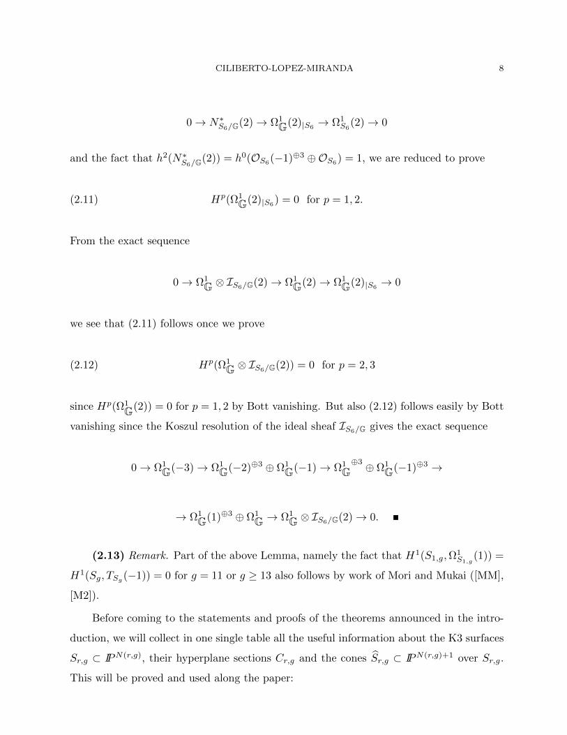
CILIBERTO-LOPEZ-MIRANDA 8
0→ N∗S6/G(2)→ Ω1G(2)|S6
→ Ω1S6
(2)→ 0
and the fact that h2(N∗S6/G(2)) = h0(OS6(−1)⊕3 ⊕OS6
) = 1, we are reduced to prove
(2.11) Hp(Ω1G(2)|S6
) = 0 for p = 1, 2.
From the exact sequence
0→ Ω1G ⊗ IS6/G(2)→ Ω1
G(2)→ Ω1G(2)|S6
→ 0
we see that (2.11) follows once we prove
(2.12) Hp(Ω1G ⊗ IS6/G(2)) = 0 for p = 2, 3
since Hp(Ω1G(2)) = 0 for p = 1, 2 by Bott vanishing. But also (2.12) follows easily by Bott
vanishing since the Koszul resolution of the ideal sheaf IS6/G gives the exact sequence
0→ Ω1G(−3)→ Ω1
G(−2)⊕3 ⊕ Ω1G(−1)→ Ω1
G⊕3 ⊕ Ω1
G(−1)⊕3 →
→ Ω1G(1)⊕3 ⊕ Ω1
G → Ω1G ⊗ IS6/G(2)→ 0.
(2.13) Remark. Part of the above Lemma, namely the fact that H1(S1,g,Ω1S1,g
(1)) =
H1(Sg, TSg(−1)) = 0 for g = 11 or g ≥ 13 also follows by work of Mori and Mukai ([MM],
[M2]).
Before coming to the statements and proofs of the theorems announced in the intro-
duction, we will collect in one single table all the useful information about the K3 surfaces
Sr,g ⊂ IPN(r,g), their hyperplane sections Cr,g and the cones Sr,g ⊂ IPN(r,g)+1 over Sr,g.
This will be proved and used along the paper:

CLASSIFICATION OF VARIETIES WITH CANONICAL CURVE SECTION 9
Table (2.14)
r g corank ΦωCr,gh0(NCr,g
(−2)) bound on h0(NSr,g
) hypothesis on Sr,g hypothesis on Cr,g
1 6 10 ≤ 1 85 general general
1 7 9 0 98 general general
1 8 7 0 114 general general
1 9 5 0 132 general general
1 10 4 0 153 general general
1 11 1 0 general general
1 12 2 0 201 general general
1 ≥ 13 1 0 general general
1 ≥ 17 1 0 general any smooth
2 2 13 any smooth any smooth
2 3 10 ≤ 1 139 any smooth any smooth
2 4 7 0 234 any smooth any smooth
2 5 4 0 363 non trigonal any smooth
2 6 2 0 525 Cliff ≥ 2 any smooth
2 ≥ 7 1 0 general any smooth
3 2 10 1 smooth ramif. div. general
3 2 18 1 smooth ramif. div. special
3 3 5 0 any smooth any smooth
3 4 2 0 889 any smooth any smooth
3 ≥ 5 1 0 any smooth any smooth
4 2 1 0 smooth ramif. div. any smooth
4 3 2 0 1209 any smooth any smooth
4 ≥ 4 1 0 any smooth any smooth
≥ 5 2 1 0 smooth ramif. div. any smooth
≥ 5 ≥ 3 1 0 any smooth any smooth
Note that the empty spaces in column 5 of the above table correspond to the cases
were there are no threefolds with the given r and g.
We now prove the main result of the section, which is the announced computation of

CILIBERTO-LOPEZ-MIRANDA 10
the corank of the Gaussian map.
Theorem (2.15). For r ≥ 1 and g ≥ 2 let Sr,g be a smooth K3 surface representing
a point of Hr,g and Cr,g a smooth hyperplane section of Sr,g. Then under the hypotheses
on Sr,g and Cr,g given in columns 6 and 7 of Table (2.14), the values of corank ΦωCr,gare
given in column 3.
Proof: For r = 1, g ≥ 6 and Cr,g general the corank of the Gaussian map ΦωCr,gwas
already computed in previous articles: for 6 ≤ g ≤ 9 or g = 11 it was done in [CM1]; for
g = 10 in [CU]; for g ≥ 12 in Theorem 4 and Proposition 3 of [CLM1]. Now consider r
and g as in the table below
Table (2.16)
r g
1 ≥ 17
2 ≥ 7
3 ≥ 5
4 2 or ≥ 4
≥ 5 ≥ 2
and Cr,g any smooth hyperplane section of Sr,g. In all these cases, using the main result
of [CLM2], it easily follows that corank ΦωCr,g= 1 : By Theorem 1.1 and Remark 2.7 of
[CLM2] we have that the Gaussian map ΦOSr,g (1) is surjective for the values of r and g in
Table (2.16). Under the same hypotheses from Lemma (2.3) we have that φr,g = φr,g,1 is
surjective. Hence Lemma (2.2) gives that ΦωCr,ghas corank one.
It remains to compute the corank of ΦωCr,gin the lower genera. For g ≥ 3 we have
that Sr,g = vr(Sg), where vr is the r-th Veronese embedding, hence corank ΦωCr,g=
corank ΦωC′ where C ′ is a smooth curve cut out on Sg by an hypersurface of degree r.
When 3 ≤ g ≤ 5 the K3 surface Sg is a complete intersection, hence so is C ′ and the corank
of the Gaussian map of C ′ can be computed by a result of Wahl as follows. If C ′ ⊂ IP g is a
complete intersection of type (d1, . . . , dg−1), setting k =g−1∑j=1
dj − g − 1 we have a diagram

CLASSIFICATION OF VARIETIES WITH CANONICAL CURVE SECTION 11
(2.17)
∧2H0(IP g,OIP g (k))
ΦOIPg (k)−→ H0(IP g,Ω1IP g (2k))
↓ φk↓ πk H0(C ′,Ω1
IP g (2k)|C′)↓ ψk∧2
H0(C ′, ωC′)Φω
C′−→ H0(C ′, ω⊗3C′ )
and πk is surjective since H1(IC′(k)) = 0, ΦOIPg (k) is surjective by [W, Theorem 6.4], φk
is surjective if 2k 6= dj , ∀j = 1, . . . , g − 1 ([W, Proposition 6.6]). In the cases at hand the
(g − 1)-tuples (d1, . . . , dg−1) are given by the following
Table (2.18)
(d1, . . . , dg−1) g r k
(2, 2, 2, 2) 5 2 2
(2, 2, 3) 4 2 2
(2, 3, 3) 4 3 3
(2, 4) 3 2 2
(3, 4) 3 3 3
(4, 4) 3 4 4
thus we see that 2k 6= dj (and φk is surjective) except for the case (2, 4). For the map
ψk : H0(Ω1IP g |C′(2k)) → H0(Ω1
C′(2k)) we get corank ψk = H1(N∗C′/IP g (2k)) as long as
H1(Ω1IP g |C′(2k)) = 0. From the Euler sequence
0→ Ω1IP g |C′(2k)→ H0(OC′(1))⊗OC′(2k − 1)→ OC′(2k)→ 0
and the fact that H1(OC′(2k−1)) = H0(OC′(1−k))∗ = 0 we see that H1(Ω1IP g |C′(2k)) = 0
since the multiplication map H0(OC′(2k−1))⊗H0(OC′(1))→ H0(OC′(2k)) is surjective.
Excluding the case (2, 4) for the moment, by (2.17) we have
corank ΦωC′ = corank ψk = h1(N∗C′/IP g (2k)) = h0(NC′/IP g (−k)) =
g−1∑j=1
h0(OC′(dj − k))
and this gives the required values. In the case (2, 4), C ′ = Q ∩ S3 ⊂ IP 3 with Q a quadric
surface, and
Claim (2.19). In diagram (2.17) we have:
(i) corank φ2 = 1;

CILIBERTO-LOPEZ-MIRANDA 12
(ii) corank ψ2 = 10;
(iii) Ker ψ2 6⊆ Im φ2.
By Claim (2.19) we deduce that corank ΦωC′ = corank ΦωC′ π2 = corank ψ2 φ2
ΦOIP3 (2) = corank ψ2 φ2 = corank ψ2 = 10.
Proof of Claim (2.19): By the above computation corank ψ2 = h0(OC′) + h0(OC′(2)) =
1 + g(C ′) = 10, hence (ii). From the exact sequence
0→ Ω1IP 3 ⊗ IC′(4)→ Ω1
IP 3(4)→ Ω1IP 3(4)|C′ → 0
we see that corank φ2 = h1(Ω1IP 3 ⊗ IC′(4)) since H1(Ω1
IP 3(4)) = 0. Tensoring by Ω1IP 3(4)
the Koszul resolution of IC′ we have
0→ Ω1IP 3(−2)→ Ω1
IP 3(2)⊕ Ω1IP 3 → Ω1
IP 3 ⊗ IC′(4)→ 0
and therefore h1(Ω1IP 3 ⊗ IC′(4)) = 1 by Bott vanishing, hence (i). To see (iii) consider the
following diagram
0→ H0(N∗S3(4))
f−→ H0(Ω1IP 3 |S3
(4))
φ3
↓ π H0(Ω1IP 3(4))
φ2
0→ H0(N∗C′(4))g−→ H0(Ω1
IP 3 |C′(4))
where Im f = Ker ψ3 : H0(Ω1IP 3 |S3
(4)) → H0(Ω1S3
(4)) ∼= C and Im g = Ker ψ2 and
π is the restriction map. By [CLM2, proof of Theorem 1.1] we know that corank φ3 = 1
and that, if F is a generator of Ker ψ3, we have that f(F ) 6∈ Im φ3. If we let F ′ ∈
H0(N∗C′(4)) be such that g(F ′) = π(f(F )) it follows that g(F ′) 6∈ Im φ2 and hence that
Ker ψ2 6⊆ Im φ2. For otherwise, since corank φ3 = 1, we have that Im π ⊆ Im φ2 and
this contradicts (i) since π is surjective, as it can be easily seen by Bott vanishing. This
proves Claim (2.19).
In the case g = 6, r = 2 and CliffS2,6 ≥ 2, that is when C ′ = S6 ∩Q ⊂ IP 6, with Q
a quadric hypersurface and CliffS6 ≥ 2, we have a diagram∧2H0(S6,OS6
(2))ΦOS6
(2)
−→ H0(S6,Ω1S6
(4))↓ φS6
↓ πS6H0(C ′,Ω1
S6(4)|C′)
↓ ψS6∧2H0(C ′, ωC′)
ΦωC′−→ H0(C ′, ω⊗3
C′ )

CLASSIFICATION OF VARIETIES WITH CANONICAL CURVE SECTION 13
and
Claim (2.20). In the above diagram we have:
(i) πS6and ΦOS6
(2) are surjective;
(ii) corank ψS6 ≤ 1;
(iii) corank φS6= 1.
From Claim (2.20) it follows that corank ΦωC2,6= corank ΦωC′ = corank ψS6
φS6≤ 2.
On the other hand if corank ΦωC2,6≤ 1 then H0(NC2,6(−2)) = 0 since C2,6 is a canonical
curve: this follows by [CM1, Lemma 1.10] in the case corank ΦωC2,6= 0 and by [CM2,
Lemma 5.2] in the case corank ΦωC2,6= 1. By a theorem of Zak (see [Z], [B], [BEL] or
[L]) we have that C2,6 ⊂ IP 20 is not 2-extendable, that is there is no threefold V ⊂ IP 22
different from a cone such that C2,6 = V ∩ IP 20. But this contradicts the fact that the K3
surface S6 ⊂ IP 6 is a quadric section of a threefold V3 ⊂ IP 6 : V3 = G ∩ H1 ∩ H2 ∩ H3
where G = G(1, 4) ⊂ IP 9 is the Grassmannian of lines in IP 4 in the Plucker embedding
and the Hi’s are hyperplanes. Therefore C2,6 = v2(S6) ∩ H ′ = v2(V3) ∩ H ′ ∩ H ′′ (with
H ′, H ′′ hyperplanes).
Proof of Claim (2.20): As above we have dim Coker ψS6≤ h1(N∗C′/S6
(4)) = h1(OC′(2)) =
h1(ωC′) = 1, that is (ii). For (iii) observe that dim Coker φS6= h1(Ω1
S6(2)) = 1 by Lemma
(2.3). Also the map πS6 is surjective since it is the restriction map and H1(IC′/S6(2)) =
H1(OS6) = 0. The fact that ΦOS6(2) or equivalently ΦOS2,6
(1) is surjective has been proved
in [CLM2, proof of Theorem 1.1] and this gives (i). This ends the proof of the Claim (2.20).
To finish the proof of the theorem let us consider the cases g = 2, r = 2, 3. For g = 2
the K3 surface S2 is a double cover of IP 2 given by a linear system |H| with H2 = 2 and the
curve C ′ ∼= Cr,2 is a smooth member of |rH|. For r = 2 we have that C2,2 is a hyperelliptic
curve of genus 5, hence corank ΦωC2,2= 13 by [CM2, Proposition 1.1] or [W, Remark
5.8.1]. When r = 3 a general member C3,2 of |3H| is isomorphic to a smooth plane sextic,
hence corank ΦωC3,2= 10 by [CM2, section 2], while the special members have a 2:1 map
onto a smooth plane cubic, hence corank ΦωC3,2= 18 by [CM2, Corollary 3.3].
This then concludes the proof of Theorem (2.15).
(2.21) Remark. Note that in the case r = 3, g = 2 of Theorem (2.15), the corank
of the Gaussian map ΦωC3,2is not constant in the linear system |OS3,2
(1)|. On the other

CILIBERTO-LOPEZ-MIRANDA 14
hand using a diagram like (2.1) it is easy to deduce, as in Lemma (2.2), that if S is a
smooth K3 surface, L is an effective line bundle on S and we have ΦL surjective and
H1(S,Ω1S ⊗ L) = 0, then, for every smooth C ∈ |L|, the corank of ΦωC
is one. It is an
interesting question to find better hypotheses that insure the constancy of the corank of
ΦωCin a given linear system on a smooth K3 surface. The other intriguing feature is
that the example given above of non constancy of the corank of the Gaussian map is the
same as Donagi-Morrison’s (essentially unique, see [CP]) example of non constancy of the
gonality of the smooth curves in a linear system on a K3 surface.
Before the end of this section we will also prove a result about the Gaussian maps
ΦωCr,g ,ω⊗kCr,g
that will be useful in the next section.
Proposition (2.22). Fix r ≥ 1 and g ≥ 2. Assume that Sr,g and Cr,g satisfy the
hypotheses given in columns 6 and 7 of Table (2.14). Then the Gaussian map ΦωCr,g ,ω⊗kCr,g
is surjective for every k ≥ 2 except for k = 2 and (r, g) = (2, 3), (1, 6), (3, 2). Moreover if
NCr,g is the normal bundle of Cr,g in IPH0(Cr,g,OCr,g (1))∗, then h0(NCr,g (−2)) is given
by column 4 of Table (2.14) and h0(NCr,g (−k)) = 0 for every k ≥ 3.
Proof: Set C = Cr,g and S = Sr,g. Since C is a canonical curve it is well known that, for
k ≥ 2, we have
Coker ΦωC ,ω⊗kC
∼= H0(NC(−k))∗
(see for example [CM1, Proposition 1.2]), hence the assertion on surjectivity of ΦωCr,g ,ω⊗kCr,g
follows by proving the vanishing of h0(NCr,g (−k)). For r = 1, g ≥ 6 and C general the
values of h0(NC(−k)) are given in Lemma 4 of [CLM1]. Suppose now r ≥ 2, g ≥ 3
or r ≥ 5, g = 2 and C any smooth hyperplane section of S. Set R(OS(1),OS(k)) =
Ker H0(OS(1))⊗H0(OS(k))→ H0(OS(k + 1)) and consider the diagram
R(OS(1),OS(k))ΦOS(1),OS(k)−→ H0(S,Ω1
S(k + 1))↓ φ
↓ π H0(C,Ω1S(k + 1)|C)↓ ψ
R(OC(1),OC(k))Φ
ωC,ω⊗kC−→ H0(C,ωC(k + 1)).
Since ΦOS(1),OS(k) is surjective by [CLM2, Theorem 1.1 and Remark 2.7; note that for r =
2, g = 5, 6 the proof of Theorem 1.1 works just assuming S2,5 non trigonal or CliffS2,6 ≥

CLASSIFICATION OF VARIETIES WITH CANONICAL CURVE SECTION 15
2], and ψ is surjective because Coker ψ ⊆ H1(N∗C/S(k + 1)) = H1(OC(k)) = 0 for k ≥ 2,
it follows that
corank ΦωC ,ω⊗kC≤ corank φ = h1(S,Ω1
S(k)) =
0 for (k, r, g) 6= (2, 2, 3)1 for (k, r, g) = (2, 2, 3)
by Lemma (2.3).
For g = 2, r = 3 the values of h0(NC(−k)) are in [CM2, section 2] for C general
and in [CM2, Theorem 3.2] for C special. For r = 1, g ≥ 17 or r = 4, g = 2 we have
corank ΦωC= 1 by Theorem (2.15), hence h0(NC(−k)) = 0 for k ≥ 2 (k = 2 by [CM2,
Lemma 5.2]).
(2.23) Remark. In the case r = 1, g ≥ 17 Theorem (2.15) is a generalization of the
Corank One Theorem of [CLM1] (Theorem 4) since there the fact that corank ΦωCg= 1
was proved for a general hyperplane section Cg of a general prime K3 surface Sg, while
here the same holds for any smooth hyperplane section C1,g of a general Sg. On the other
hand it should be noticed that the proof of this fact is not independent of Theorem 4 of
[CLM1] as the latter is used to deduce the corank one from the surjectivity of ΦOSg (1) (in
Lemma (2.3)). Alternatively one can avoid using Theorem 4 of [CLM1] by invoking results
of Mori and Mukai ([MM], [M2]); see remark (2.13).
3. VARIETIES WITH CANONICAL CURVE SECTION
We begin by recalling Zak’s theorem mentioned in the introduction. A smooth non-
degenerate variety X ⊂ IPm is said to be k-extendable if there exists a variety Y ⊂ IPm+k
that is not a cone and such that X = Y ∩ IPm. Zak’s theorem says that if codim X ≥ 2,
h0(NX(−1)) ≤ m + k and h0(NX(−2)) = 0, then X is not k-extendable. For a canonical
curve C ⊂ IP g−1 one has also h0(NC(−1)) = g + corank ΦωC([CM1, Proposition 1.2]),
hence the knowledge of corank ΦωC(and of h0(NC(−2)) that is also given by a Gaussian
map) gives information on the possibility of extending C.
Next we consider a smooth nondegenerate variety X ⊂ IPm of dimension n ≥ 3
such that its general curve sections C are canonical curves. By a well-known equivalence
criterion we must have −KX = (n − 2)H, where H is the hyperplane divisor. Hence a
general surface section S is a K3 surface, and therefore S = Sr,g, C = Cr,g for some r, g.

CILIBERTO-LOPEZ-MIRANDA 16
We denote such an X by Xnr,g. When n = 3 we denote Vr,g = X3
r,g. Note that Vr,g ⊂
IPN(r,g)+1 = IPH0(Vr,g,−KVr,g)∗ is anticanonically embedded and, by Riemann-Roch,
N(r, g) = h0(Vr,g,−KVr,g ) − 2 = − 12K
3Vr,g
+ 1 = 1 + r2(g − 1) = 12dr
3 + 1, where H =
r∆, d = ∆3.
These varieties Xnr,g have been extensively studied, both in dimension three (Fano,
Iskovskih [I1], [I2], etc.) and in dimension n ≥ 4 (Mukai [M1], [M2]). Observe that by
applying some basic adjunction theory (e.g. [KO]) we can divide the varieties Xnr,g in
two categories (with two exceptions): (a) n = 3 and r ≥ 1, that is Fano threefolds of
index r; (b) n ≥ 4 and r = 1, that is Fano manifolds of dimension n ≥ 4 and index
1. In fact for n ≥ 4, r ≥ 2 the only possible values are n = 4, 5, r = 2 and (X,∆) =
(Q,OQ(1)), (IP 5,OIP 5(1)), where Q is a smooth quadric in IP 5, since in all other cases we
have r(n − 2) > n + 1. Even though we will not make use of adjunction theory in our
proofs, the interesting cases are (a) and (b) above.
The case of Fano threefolds of index one was already treated in [CLM1], thus from
now on we will assume r ≥ 2 or n ≥ 4.
Given r ≥ 2 and g ≥ 2, we will denote by Vr,g the Hilbert scheme of smooth Fano
threefolds Vr,g ⊂ IPN(r,g)+1 of index r, anticanonically embedded and by Vr,g,1 the closure
in Vr,g of the locus of Fano threefolds with Picard number one.
We now present a list of examples taken from the papers of Fano and Iskovskih of
families of Fano threefolds Vr,g of the principal series and of index greater than one (see
e.g. [M]):
Table (3.1)
r g d = ∆3 N(r, g) number of parameters Vr,g
4 3 1 33 1209 IP 3
3 4 2 28 889 quadric in IP 4
2 3 2 9 139 double cover of IP 3 ramified along a quartic
2 4 3 13 234 cubic in IP 4
2 5 4 17 363 complete intersection of two quadrics in IP 5
2 6 5 21 525 G(1, 4) ∩ IP 6 ⊂ IP 9
Our first classification result is the following:

CLASSIFICATION OF VARIETIES WITH CANONICAL CURVE SECTION 17
Theorem (3.2). Fix r ≥ 2 and g ≥ 2. Then we have:
(i) Vr,g = ∅ for (r, g) such that: r = 2, g = 2 or g ≥ 11; r = 3, g = 2, 3 or g ≥ 5;
r = 4, g = 2 or g ≥ 4; r ≥ 5, g ≥ 2; r = 2, 7 ≤ g ≤ 10 assuming furthermore that the
hyperplane section S2,g of V2,g is non trigonal and non DP;
(ii) Vr,g,1 = ∅ for (r, g) not in Table (3.1);
(iii) For (r, g) as in Table (3.1) Vr,g,1 is irreducible and the families of Fano-Iskovskih
form a dense open subset of smooth points of Vr,g,1.
(3.3) Remark. Theorem (3.2) characterizes the set of integers (r, g) with r ≥ 2, g ≥ 2
for which Vr,g,1 is non empty, that is when there exists a smooth Fano threefold Vr,g
with Picard number one. Moreover it gives, in (iii), a characterization of the general such
Vr,g. In fact it is true that any Vr,g (with Picard number one) is one of the examples of
Fano-Iskovskih (see [I1], [I2], [M]).
(3.4) Remark. Part (i) of Theorem (3.2) can be summarized in the following diagram
≥ 5∣∣ x x x x x x x x x x
4∣∣ x • x x x x x x x x
3∣∣ x x • x x x x x x x
2∣∣ x • • • • tdp tdp tdp tdp x
r / g∣∣ 2 3 4 5 6 7 8 9 10 ≥ 11
where x means that there is no Vr,g, • means that there is one and tdp means that there is
no Vr,g with trigonal or DP hyperplane section Sr,g. In fact again from the classification
of Iskovskih it is true that Vr,g = ∅ also for r = 2, g = 9, 10. For r = 2, g = 7, 8 instead
there are Fano threefolds, but with Picard number two or three (see [I1], [I2], [M]).
Proof of Theorem (3.2): Suppose first g = 2. Then d = 2(g−1)/r = 2/r is an integer only if
r = 2, but then for the K3 surface S2,2 we have that OS2,2(1) = OS2,2
(2∆|S2,2) ∼= OS2
(2D)
where φD gives the 2:1 map onto IP 2. But this is a contradiction since on S2 the line
bundle OS2(2D) is not very ample. Similarly for r = g = 3 we have that d is not an
integer. For r = 3, g ≥ 5 or r = 4, g ≥ 4 or r ≥ 5, g ≥ 3, we have by Theorem (2.15) that
corank ΦωCr,g= 1, hence by [CM1, Proposition 1.2] h0(NCr,g (−1)) = N(r, g) + 1. Also
h0(NCr,g(−2)) = 0 by [CM2, Lemma 5.2], and therefore Zak’s theorem implies that Cr,g
is not 2-extendable, hence that Vr,g = ∅ for the above values of r and g. For r = 2, g ≥ 7

CILIBERTO-LOPEZ-MIRANDA 18
observe that, as in the proof of Lemma (2.3), for the K3 surface S2,g = v2(Sg) ⊂ IPN(2,g)
we have h1(TS2,g(−α)) = h1(TSg
(−2α)), α = 1, 2, hence
(3.5)
h0(NS2,g (−α)) =
N(2, g) + 1 + h1(TSg (−2)) = N(2, g) + 1 + h0(NSg (−2)) for α = 1h1(TSg (−4)) = h0(NSg (−4)) for α = 2
.
By Zak’s theorem to show that V2,g does not exist under the hypotheses given in (i) is
then enough to prove that h0(NSg(−2)) = 0. Now let Cg be a general hyperplane section
of Sg; as in (2.10) we have
(3.6) h0(NSg (−2α)) ≤∑h≥0
h0(NCg/IP g−1(−2α− h)).
Since h0(NCg/IP g−1(−2)) = corank ΦωCg ,ω⊗2Cg
we only need to check that ΦωCg ,ω⊗2Cg
is sur-
jective. But this follows by [BEL, Theorem 2] for CliffCg ≥ 3 and by the results of [T,
Theorems 2.10 and 2.6] for CliffCg = 1, 2 except when Cg is bielliptic. But the latter
case cannot happen by [CP, Corollary 2.5 and Theorem 3.1]; it can also be excluded by
[CvdG]. This proves (i). To see (ii) and (iii) we will use the following
Lemma (3.7). Suppose Vr,g has Picard number one. Then a general hyperplane
section Sr,g of a general deformation of Vr,g is represented by a general point of Hr,g.
Proof of Lemma (3.7): Set V = Vr,g, S = Sr,g and consider the usual deformation diagram
H1(V, TV )αS−→ H1(S, TV|S ) → H2(V, TV (−1))
γS−→ H2(V, TV ) → H2(S, TV|S )↑ βS
H1(S, TS)
First we prove
(3.8) βS is surjective;
(3.9) h2(V, TV (−1)) = 1;
(3.10) H2(V, TV ) = 0.
In fact the map βS comes from the exact sequence
(3.11) 0→ TS → TV|S → NS/V → 0
hence Coker βS ⊆ H1(NS/V ) = H1(OS(1)) = 0, that is (3.8). By Serre duality we get
h2(V, TV (−1)) = h1(Ω1V ) = 1 since OV (1) = OV (−KV ) and V has Picard number one.

CLASSIFICATION OF VARIETIES WITH CANONICAL CURVE SECTION 19
This proves (3.9). To see (3.10) observe that by (3.11) we have H2(TV |S) = 0, hence if
H2(TV ) 6= 0 we necessarily have h2(TV ) = 1 and γS is surjective. On the other hand
γS is given by multiplication with the equation of the hyperplane defining S, hence the
multiplication map µ : H0(OV (1)) ⊗H2(TV (−1)) → H2(TV ) is surjective. But then, by
Bertini’s theorem, there is a smooth surface S′ in the codimension one sublinear system
Ker µ ⊂ H0(OV (1)). Replacing S with S′ we get that γS′ is the zero map, and this
contradicts the hypothesis that H2(TV ) 6= 0. Alternatively (3.10) follows by Kodaira-
Nakano vanishing since H2(TV ) ∼= H1(Ω1V (KV )) = H1(Ω1
V (−1)) = 0.
Now by (3.10) every infinitesimal deformation of V is unobstructed and by (3.9) we
have that dim Coker αS = 1, hence every infinitesimal algebraic deformation of S comes
from a deformation of V . This proves Lemma (3.7).
To see (ii) of Theorem (3.2) by Lemma (3.7) we can assume that Sr,g is general.
Moreover note that if (r, g) are not in Table (3.1) and the existence of Vr,g is not excluded
by (i), we have r = 2, g ≥ 7. Therefore by Theorem (2.15) we have again corank ΦωCr,g= 1,
hence we conclude as above that Vr,g,1 = ∅. This gives (ii).
To see (iii) observe that the Fano threefolds Vr,g of the principal series are projectively
Cohen-Macaulay, hence they flatly deform to the cone Sr,g over their hyperplane section
Sr,g, and similarly for Sr,g to the cone Cr,g over Cr,g. Setting V = Vr,g, S = Sr,g, C =
Cr,g, N = N(r, g) and denoting by Tr,g the tangent space to Vr,g,1 at the point representing
Vr,g, we have
(3.12) dim Tr,g = h0(NV/IPN+1) ≤ h0(NS/IPN+1) =
∑h≥0
h0(NS/IPN (−h)) ≤
≤ h0(NS/IPN ) +∑h≥1
h0(NC/IPN (−h)) = h0(NS/IPN ) +
∑h≥1,j≥0
h0(NC/IPN−1(−h− j)) =
= h0(NS/IPN ) + h0(NC/IPN−1(−1)) + 2h0(NC/IPN−1(−2))
by Proposition (2.22). As we know h0(NS/IPN ) = dim Hr,g = 18 + (N + 1)2 and
h0(NC/IPN−1(−1)) = N + corank ΦωChence we deduce that
(3.13) h0(NS/IPN ) + h0(NC/IPN−1(−1)) + 2h0(NC/IPN−1(−2)) = f(r, g) :=
= N(r, g)2 + 3N(r, g) + 19 + corank ΦωCr,g+ 2h0(NCr,g (−2)).

CILIBERTO-LOPEZ-MIRANDA 20
By Theorem (2.15), Proposition (2.22) and Table (3.1) we see that f(r, g) is equal to the
number of parameters of the examples of Fano-Iskovskih. By (3.12) and (3.13) we also
have that f(r, g) is an upper bound for h0(NS/IPN+1), hence the argument presented in
the Introduction applies and we conclude that Vr,g,1 is irreducible and that the families of
Fano-Iskovskih form a dense open subset of smooth points.
We now turn to the higher dimensional case and classify the Mukai varieties. For
n ≥ 4, r ≥ 1 and g ≥ 2 we let Xn,r,g be the Hilbert scheme of smooth Fano n-folds
Xnr,g ⊂ IPN(r,g)+n−2 of index r(n−2) and Xn,r,g,1 the closure in Xn,r,g of the locus of Fano
n-folds with Picard number one.
For Fano manifolds of dimension n ≥ 4 and index r(n − 2), of the principal series
and with Picard number one, we present the list given by Mukai ([M1], [M2]) of examples
of families of such Xnr,g. Of course, since the general hyperplane section of an Xn
r,g is an
Xn−1r,g , we only present the list of the maximum dimensional varieties. There is one family
for each genus g ≥ 6 (for r = 1, g ≤ 5 they are complete intersections) and we denote the
maximum dimension of the examples in the list by n(g):
Table (3.14)
r g n(g) number of parameters Xn(g)r,g
1 6 6 145 ˜G(1, 4) ∩Q ⊂ IP 10
1 7 10 210 SO(10,C)/P ⊂ IP 15
1 8 8 189 G(1,5) ⊂ IP 14
1 9 6 174 Sp(6,C)/P ⊂ IP 13
1 10 5 181 G2/P ⊂ IP 13
2 5 5 405 v2(IP 5) ⊂ IP 20
For 4 ≤ n < n(g) Mukai shows that any Xn1,g is a linear section of the X
n(g)1,g .
Our final result gives the classification as follows:
Theorem (3.15). Fix n ≥ 4, r = 1 and g ≥ 6 or r ≥ 2 and g ≥ 2. Then we have:
(i) Xn,r,g = ∅ for (r, g) such that: r ≥ 3, g ≥ 2; r = 2 and 2 ≤ g ≤ 4 or g ≥ 8 or
g = 5, 6, n ≥ 6 or g = 6, n ≥ 4 and CliffS2,6 ≥ 2 or g = 7 and S2,7 non trigonal and
non DP;

CLASSIFICATION OF VARIETIES WITH CANONICAL CURVE SECTION 21
(ii) Xn,r,g,1 = ∅ for (r, g) not in Table (3.14) or for (r, g) in Table (3.14) and n > n(g);
(iii) For (r, g) as in Table (3.14) and 4 ≤ n ≤ n(g) we have that Xn,r,g,1 is irreducible
and the examples of families of Mukai form a dense open subset of smooth points of
Xn,r,g,1.
Proof: By (i) of Theorem (3.2) to prove (i) of Theorem (3.15) we need to consider the cases
r = 2 and 3 ≤ g ≤ 10, g 6= 7, r = 3 and g = 4 or r = 4 and g = 3. For (r, g) = (3, 4) and
(r, g) = (4, 3) we have by Theorem (2.15) that corank ΦωCr,g= 2 and h0(NCr,g (−2)) = 0
by Proposition (2.22), hence Cr,g is not 3-extendable by Zak’s theorem. Similarly for
r = 2, g = 5 (respectively g = 6) and S2,5 non trigonal (respectively CliffS2,6 ≥ 2), we
have corank ΦωC2,5= 4 (respectively corank ΦωC2,6
= 2) and h0(NCr,g(−2)) = 0, hence
C2,5 is not 5-extendable (respectively C2,6 is not 3-extendable). For r = 2, g = 5, 6 and
S2,5 trigonal or CliffS2,6 = 1 we have instead by [T, Theorems 2.6 and 2.4] and [CM2,
Theorem 2.3] that corank ΦωCg ,ω⊗2Cg
≤ 3, h0(NCg(−3)) = 0, hence S2,g is not 4-extendable
by (3.5) and (3.6). The same argument shows that, for 8 ≤ g ≤ 10, S2,g is not 2-extendable
since in this case corank ΦωCg ,ω⊗2Cg
≤ 1, h0(NCg (−3)) = 0 again by [BEL, Theorem 2], [T,
Theorems 2.4, 2.6, 2.10 and 1.7] and [CM2, Theorems 3.2 and 3.4]. For r = 2, g = 4 we
have deg Xn2,4 = deg C2,4 = 2N(2, 4)−2 = 24 and OXn
2,4(1) = OXn
2,4(2∆), hence 2n∆n = 24
and therefore n ≤ 3. For r = 2, g = 3 if there exists an X42,3 we get deg X4
2,3 = deg C2,3 =
2N(2, 3) − 2 = 16 = 24∆4, hence ∆4 = 1. By restricting to the surface section S2,3 one
easily checks that |∆| is base point free, birational and h0(OX42,3
(∆)) = 4 and this of course
is a contradiction. Alternatively we can exclude the existence of a smooth X42,3 using some
basic adjunction theory: we have −KX42,3
= 4∆, with H = 2∆, hence ∆ is ample; by [KO]
it must be (X42,3,OX4
2,3(∆)) ∼= (Q,OQ(1)) where Q is a smooth quadric in IP 5, but this
contradicts the fact that h0(OX42,3
(1)) = h0(OX42,3
(2∆)) = 12 while h0(OQ(2)) = 20. This
proves (i).
To see part (ii), by part (i) which was just proved and by (ii) of Theorem (3.2)(and
by Lemma (3.7)), it remains to consider the cases r = 1, g ≥ 6. Let r = 1, 7 ≤ g ≤ 10.
We notice that by [CLM1, Lemma 4] one has h0(NC1,g(−2)) = 0, hence Zak’s theorem
applies, and therefore if we set ν := corank ΦωC1,g+ 1, then C1,g is not ν-extendable. On
the other hand ν is computed in [CLM1, Table 2] and is equal to n(g). Hence we conclude

CILIBERTO-LOPEZ-MIRANDA 22
that Xn,r,g,1 = ∅ for r = 1, 7 ≤ g ≤ 10 and n > n(g). For r = 1 and g ≥ 11 by [CLM1,
Theorem 4, Lemma 4 and Table 2] we have corank ΦωC1,g≤ 2 and h0(NC1,g
(−2)) = 0,
hence C1,g is not 3-extendable.
For r = 1, g = 6 we have corank ΦωC1,6= 10 by [CLM1, Table 2] but in fact there is
no smooth X71,6 in this case (note that h0(NC1,6
(−2)) 6= 0 !). To see this observe first that,
by (iii) below, a general smooth X61,6 is the intersection of a quadric hypersurface Q ⊂ IP 10
and the cone G over the Grassmannian G = G(1, 4) ⊂ IP 9 in the Plucker embedding. Now
suppose there is X71,6 ⊂ IP 11. Then an argument like Lemma (3.7) shows that a general
hyperplane section of a general deformation of the X71,6 is a general X6
1,6, hence such that
X61,6 = G ∩ Q = X7
1,6 ∩ H. Since the ideal of G ⊂ IP 9 is generated by five quadrics we
have H0(IG(2)) =< Q1, . . . , Q5 >, and from this it follows that also the ideals of X61,6
and X71,6 are generated by quadrics. In fact if we set IP 9 = x10 = x11 = 0 ⊂ IP 11 we
have H0(IX61,6
(2)) =< Q1, . . . , Q5, Q > and H0(IX71,6
(2)) =< Q1, . . . , Q5, Q >, where Qi
and Q are quadrics in IP 11 that restrict to Qi and Q respectively for x11 = 0. But then
the variety Y ⊂ IP 11 of dimension 8 and degree 5 defined scheme-theoretically by the five
quadrics Qi, i = 1, . . . , 5, is a variety that extends twice the Grassmannian G ⊂ IP 9 and
hence Y must be a cone over G with vertex a line (this follows for example from [CLM3]),
and then X71,6 is singular. Therefore (ii) is proved.
As in the proof of part (iii) of Theorem (3.2), using successive degenerations to cones
over hyperplane sections, to see part (iii) of Theorem (3.15) we need to show that the
family of known examples of Xnr,g has the same dimension as the dimension of the tangent
space Tnr,g to the Hilbert scheme Xn,r,g,1 at the cone points. In this case we have
dim Tnr,g = h0(NXnr,g
) ≤ h0(NVr,g)+(n−3)h0(NVr,g
(−1))+[n−3+
(n− 3
2
)]h0(NVr,g
(−2))
since h0(NVr,g (−k)) = 0 for k ≥ 3 because h0(NCr,g (−k)) = 0 by [CLM1, Lemma 4] and
Proposition (2.22). Therefore we get
h0(NVr,g) + (n− 3)h0(NVr,g
(−1)) + [n− 3 +
(n− 3
2
)]h0(NVr,g
(−2)) ≤
≤ dim Vr,g,1 + (n− 3)h0(NCr,g(−1)) + [3n− 9 +
(n− 3
2
)]h0(NCr,g
(−2)) =

CLASSIFICATION OF VARIETIES WITH CANONICAL CURVE SECTION 23
= N(r, g)2 + nN(r, g) + 19 + (n− 2) corank ΦωCr,g+ [3n− 7 +
(n− 3
2
)]h0(NCr,g (−2)).
Now one easily sees that the values of the upper bound given above coincide with the
number of parameters of the examples of Mukai in Table (3.14) for n = n(g) or of their
hyperplane sections for n < n(g).
(3.16) Remark. Since Pinkham’s work on cones over elliptic curves it is well known
that, in general, the converse of Zak’s theorem does not hold (an elliptic normal curve of
degree at least 10 provides a counterexample). We would like to note here that from the
two theorems just proved we can deduce more examples in the case of smooth extensions,
that is smooth nondegenerate varieties X ⊂ IPm such that h0(NX(−2)) = 0 and X is not
smoothly k-extendable, but h0(NX(−1)) > m + k. Examples are given by the varieties
C2,4, C3,3, S3,3 and V2,4. Also note that in the case r = 1, g = 6 we have that C1,6 is
infinitely many times extendable (just take quadric sections of cones over G(1, 4) ⊂ IP 9
with vertices linear spaces), but it is not smoothly 6-extendable. Of course in this case we
have h0(NC1,6(−2)) 6= 0.
REFERENCES
[B] Badescu,L.: On a result of Zak-L’vovsky. Preprint No. 13/1993, Institutul de Matem-atica al Academiei Romane.
[BEL] Bertram,A., Ein,L., Lazarsfeld,R.: Surjectivity of Gaussian maps for line bundles oflarge degree on curves. In: Algebraic Geometry, Proceedings Chicago 1989. LectureNotes in Math. 1479. Springer, Berlin-New York: 1991, 15-25.
[CHM] Ciliberto,C., Harris,J., Miranda,R.: On the surjectivity of the Wahl map. Duke Math.J. 57, (1988) 829-858.
[CLM1] Ciliberto,C., Lopez,A.F., Miranda,R.: Projective degenerations of K3 surfaces, Gaus-sian maps and Fano threefolds. Invent. Math. 114, (1993) 641-667.
[CLM2] Ciliberto,C., Lopez,A.F., Miranda,R.: On the corank of Gaussian maps for generalembedded K3 surfaces. Israel Mathematical Conference Proceedings. Papers in honorof Hirzebruch’s 65th birthday, vol. 9, AMS Publications (1996), 141-157.
[CLM3] Ciliberto,C., Lopez,A.F., Miranda,R.: Some remarks on the obstructedness of conesover curves of low genus. In : Higher dimensional complex varieties, Proceedings Trento1994. De Gruyter: 1996, 167-182.
[CM1] Ciliberto,C., Miranda,R.: On the Gaussian map for canonical curves of low genus.Duke Math. J. 61, (1990) 417-443.
CILIBERTO-LOPEZ-MIRANDA 24
[CM2] Ciliberto,C., Miranda,R.: Gaussian maps for certain families of canonical curves. In:Complex Projective Geometry, Proceedings Trieste-Bergen 1989. London Math. Soc.Lecture Notes Series 179. Cambridge Univ. Press: 1992, 106-127.
[CP] Ciliberto,C., Pareschi,G.: Pencils of minimal degree on curves on a K3 surface. J.Reine Angew. Math. 460, (1995) 15-36.
[CU] Cukierman,F., Ulmer,D.: Curves of genus ten on K3 surfaces. Compositio Math. 89,no. 1, (1993) 81-90.
[CvdG] Ciliberto,C., van der Geer,G.: On the Jacobian of a hyperplane section of a surface.In : Classification of irregular varieties (Trento, 1990). Lecture Notes in Math. 1515.Springer, Berlin-New York: 1992, 33-40.
[I1] Iskovskih,V.A.: Fano 3-folds I. Math. USSR Izv. 11, (1977) 485-527.
[I2] Iskovskih,V.A.: Fano 3-folds II. Math. USSR Izv. 12, (1978) 479-506.
[KO] Kobayashi,S., Ochiai,T.: Characterizations of complex projective spaces and hyper-quadratics. J. Math. Kyoto Univ. 13, (1973) 31-47.
[L] L’vovskii,S.M.: On the extension of varieties defined by quadratic equations. Math.USSR Sbornik 63, (1989) 305-317.
[M] Murre,J.P.: Classification of Fano threefolds according to Fano and Iskovskih. In: Al-gebraic Threefolds, Proceedings Varenna 1981. Lecture Notes in Math. 947. Springer,Berlin-New York: 1982, 35-92.
[M1] Mukai,S.: Biregular classification of Fano 3-folds and Fano manifolds of coindex 3. In:Proc. Natl. Acad. Sci. USA 86. (1989), 3000-3002.
[M2] Mukai,S.: Fano 3-folds. In: Complex Projective Geometry, Proceedings Trieste-Bergen1989. London Math. Soc. Lecture Notes Series 179. Cambridge Univ. Press: 1992,255-263.
[MM] Mori,S., Mukai,S.: The uniruledness of the moduli space of curves of genus 11. In:Algebraic Geometry, Proceedings Tokyo/Kyoto 1982. Lecture Notes in Math. 1016.Springer, Berlin-New York: 1983, 334-353.
[T] Tendian,S.: Gaussian maps on trigonal and tetragonal curves. Preprint.
[W] Wahl,J.: The Jacobian algebra of a graded Gorenstein singularity. Duke Math. J. 55,(1987) 843-871.
[Z] Zak,F.L.: Some properties of dual varieties and their application in projective geome-try. In: Algebraic Geometry, Proceedings Chicago 1989. Lecture Notes in Math. 1479.Springer, Berlin-New York: 1991, 273-280.
ADDRESSES OF THE AUTHORS:
Ciro Ciliberto, Dipartimento di Matematica, Universita di Roma II, Tor Vergata,Viale della Ricerca Scientifica, 00133 Roma, Italy

CLASSIFICATION OF VARIETIES WITH CANONICAL CURVE SECTION 25
e-mail: [email protected]
Angelo Felice Lopez, Dipartimento di Matematica, Universita di Roma Tre,Via Corrado Segre 2, 00146 Roma, Italye-mail: [email protected]
Rick Miranda, Department of Mathematics, Colorado State University, Ft. Collins,CO 80523, USAe-mail: [email protected]