classification and retrieval of ... -...
TRANSCRIPT

Classification and Retrieval of Digital Pathology Scans: A New Dataset
Morteza Babaie1,2, Shivam Kalra1, Aditya Sriram1, Christopher Mitcheltree1,3,
Shujin Zhu1,4, Amin Khatami5, Shahryar Rahnamayan1,6, H.R. Tizhoosh1
1 KIMIA Lab, University of Waterloo, Canada2 Mathematics and Computer Science, Amirkabir University, Tehran, Iran3 Electrical and Computer Engineering, University of Waterloo, Canada
4 School of Electronic & Optical Eng., Nanjing University of Science & Technology, Jiangsu, China5 Institute for Intelligent Systems Research and Innovation, Deakin University, Australia
6 Electrical, Computer and Software Engineering,
University of Ontario Institute of Technology, Oshawa, Canada
Abstract
In this paper, we introduce a new dataset, Kimia Path24,
for image classification and retrieval in digital pathology.
We use the whole scan images of 24 different tissue tex-
tures to generate 1,325 test patches of size 1000×1000
(0.5mm×0.5mm). Training data can be generated accord-
ing to preferences of algorithm designer and can range from
approximately 27,000 to over 50,000 patches if the preset
parameters are adopted. We propose a compound patch-
and-scan accuracy measurement that makes achieving high
accuracies quite challenging. In addition, we set the bench-
marking line by applying LBP, dictionary approach and
convolutional neural nets (CNNs) and report their results.
The highest accuracy was 41.80% for CNN.
1. Introduction
The integration of algorithms for classification and re-
trieval in medical images through effective machine learn-
ing schemes is at the forefront of modern medicine [8].
These tasks are crucial, among others, to detect and analyze
abnormalities and malignancies to contribute to more in-
formed diagnosis and decision makings. Digital pathology
is one of the domains where such tasks can support more re-
liable decisions [23]. For several decades, the archiving of
microscopic information of specimens has been organized
through employing and storing glass slides [2]. Beyond the
fragile nature of glass slides, hospitals and clinics need large
and specially prepared storage rooms to store specimens,
which naturally requires a lot of logistical infrastructures.
Digital pathology, or whole slide imaging (WSI), can not
only provide high image quality that is not subject to decay
(i.e., stains decay over time) but also offers a range of other
benefits [2, 11]: They can be investigated by multiple ex-
perts at the same time, they can be more easily retrieved
for research and quality control, and of course, WSI can
be integrated into existing information systems of hospitals.
In 1999, Wetzel and Gilbertson developed the first auto-
mated WSI system [17], utilizing high resolution to enable
pathologists to buffer through immaculate details presented
through digitized pathology slides. Ever since, pathology
bounded by WSI systems is emerging into an era of digital
specialty, providing solutions for centralizing diagnostic so-
lutions by improving the quality of diagnosis, patient safety,
and economic concerns [12]. Like any other new technol-
ogy, digital pathology has its pitfalls. The gigapixel nature
of WSI scans makes it difficult to store, transfer, and pro-
cess samples in real-time. One also need tremendous dig-
ital storage to archive them. In this paper, we propose a
new and uniquely designed data set, Kimia Path24, for the
classification and retrieval of digitized pathology images. In
particular, the data set is comprised of 24 WSI scans of dif-
ferent tissue textures from which 1,325 test patches sized
1000×1000 are manually selected with special attention to
textural differences. The proposed data set is structured to
mimic retrieval tasks in clinical practice; hence, the users
have the flexibility to create training patches, ranging from
27,000 to over 50,000 patches – these numbers depend on
the selection of homogeneity and overlap for every given
slide. For retrieval, a weighted accuracy measure is pro-
vided to enable a unified benchmark for future works.
2. Related Works
This section covers a brief literature review on im-
age analysis in digital pathology, specifically on WSI, fol-
8
lowed by various content-based medical image retrieval
techniques, and finally an overview of feature extraction
techniques that emphasize local binary patterns (LBP).
2.1. Image Analysis in Digital Pathology
In digital pathology, the large dimensionality of the im-
age poses a challenge for computation and storage; hence,
contextually understanding regions of interest of an im-
age helps in quicker diagnosis and detection for imple-
menting soft-computing techniques [7]. Over the years,
traditional image-processing tasks such as filtering, regis-
tration, and segmentation, classification and retrieval have
gained more significance. Particularly for histopathology,
the cell structures such as cell nuclei, glands, and lympho-
cytes are observed to hold prominent characteristics that
serve as a hallmark for detecting cancerous cells [14]. Re-
searchers also anticipate that one can correlate histolog-
ical patterns with protein and gene expression, perform
exploratory histopathology image analysis, and perform
computer aided diagnostics (CADx) to provide patholo-
gists with the required support for decision making [14].
The idea behind CADx to quantify spatial histopathology
structures has been under investigation since the 1990s, as
presented by Wiend et al. [35], Bartels et al. [6], and
Hamilton et al. [16]. However, due to limited compu-
tational resources and its associated expense, implement-
ing such ideas have been overlooked or delayed. In recent
years, however, WSI technology has been gradually set-
ting laboratory standards as a process of digitizing pathol-
ogy slides to advocate for more efficient diagnostic, edu-
cational and research purposes [30]. This approach, un-
like photo-microscopy which is to capture a portion of an
image [37], offers a high-resolution overview of the entire
specimen in the slide which enables the pathologist to take
control over navigating through the slide and saving invalu-
able time [17, 36, 10, 12]. More recently, Bankhead et al.
[4] provided an open-source bio-imaging software, called
QuPath that supports WSI by providing tumor identification
and biomarker evaluation tools which developers can use to
implement new algorithms to further improve the outcome
of analyzing complex tissue images.
2.2. Image Retrieval
Retrieving similar (visual) semantics of an image re-
quires extracting salient features that are descriptive of the
image content. At its entirety, there are two main points
of view for processing the WSI scans [5]. The first one
is called sub-setting methods which considers a small sec-
tion of the huge pathology image as an important part such
that the processing of the small subset substantially reduces
processing time. The majority of research in the literature
prefers this method because of its advantage of speed and
accuracy. However, it needs expert knowledge and inter-
vention to extract the proper subset. On the other hand,
tiling methods break the images into smaller and control-
lable patches and try to process them against each other
[15]. This naturally requires more care in design and is
more expensive in execution. However, it certainly is an
obvious approach toward full automation.
Traditionally, a large medical image database is packaged
with textual annotations classified by specialists; however,
this approach does not perform well against the ever de-
manding growth of digital pathology. In 2003, Zheng et
al. [39] developed an on-line content-based image retrieval
(CBIR) system wherein the client provides a query image
and corresponding search parameters to the server side. The
server then performs similarity searches based on feature
types such as color histogram, image texture, Fourier co-
efficients, and wavelet coefficients, whilst using the vector
dot-product as a distance metric for retrieval. The server
then returns images that are similar to the query image along
with the similarity scores and a feature descriptor. Mehta et
al. [26], on the other hand, proposed an offline CBIR system
which utilizes sub-images rather than the entire histopathol-
ogy slide. Using scale-invariant feature extraction (SIFT)
[22] to search for similar structures by indexing each sub-
image, the experimental results suggested, when compared
to manual search, an 80% accuracy for the top-5 results re-
trieved from a database that holds 50 IHC stained pathology
images, consisting of 8 resolution levels. In 2012, Akakin
and Gurcan [1] developed a multi-tiered CBIR system based
on WSI, which is capable of classifying and retrieving scans
using both multi-image query and images at a slide-level.
The authors test the proposed system on 1, 666 WSI scans
extracted from 57 follicular lymphoma (FL) tissue slides
containing 3 subtypes and 44 neuroblastoma (NB) tissue
slides comprised of 4 subtypes. Experimental results sug-
gested a 93% and 86% average classification accuracy for
FL and NB diseases, respectively. More recently, Zhang et
al. [38] developed a scalable CBIR method to cope with
WSI by using a supervised kernel hashing technique which
compresses a 10,000-dimensional feature vector into only
10 binary bits, which is observed to preserve a concise rep-
resentation of the image. These condensed binary codes are
then used to index all existing images for quick retrieval for
of new query images. The proposed framework is validated
on a breast histopathology data set comprised of 3,121 WSI
scans from 116 patients; experimental results state an accu-
racy of 88.1% for processing at the speed of 10ms for all
800 testing images.
2.3. LBP Descriptor
To generate preliminary results for the introduced data
set, we captured the textural structure of patches by extract-
ing local binary patterns (LBP) [28] as they are among es-
tablished approaches proven to quantify important textures
9

in medical imaging [27, 31, 3]. We also experiment with
the dictionary approach [18, 25] and convolutional neural
networks (CNN) [21].
LBP is an extremely powerful and concise texture fea-
ture extractor, with an ability to compete with state-of-the-
art complex learning algorithms. In 2009, Masood and Ra-
jpoot [24] implemented a circular LBP (CLBP) feature ex-
traction algorithm to classify colon tissue patterns using a
Gaussian-kernel SVM on biopsy samples taken from 32
different patients. Each image has a spatial resolution of
491 × 652 × 128 pixels, for which the retrieval accuracy
is computed to be 90% to distinguish between benign and
malignant patterns. In the same year, Sertel et al. [32] pre-
sented a CADx system designed to classify Neuroblastoma
(NB) malignancy, a type of cancer in the nervous system,
using WSI. The authors proposed a multi-resolution LBP
approach which initially analyzes image at the lowest res-
olution and then switches to higher resolutions when nec-
essary. The proposed approach employs offline feature se-
lection, which enables the extraction of more discrimina-
tive features for every resolution level during the training
phase. For retrieval, a modified k-nearest neighbor is em-
ployed which when tested on 43 WSI scans, provides an
overall classification accuracy of 88.4%. More recently,
Tashk et al. [34] proposed a statistical approach based on
color information such as maximum likelihood estimation.
Then, the CLBP is employed to extract texture features
from rotational and color changes, from which the SVM
algorithm classifies the extracted feature vectors as mito-
sis and non-mitosis cases. The proposed scheme obtains
70.94% (F-measure) for Aperio XT images and 70.11% for
Hamamatsu images, both of which are microscopic scan-
ners. The reported method is observed to outperform other
participants at ICPR 2012 Mitosis detection in breast cancer
histopathological images.
3. The “Kimia Path24” Dataset
We had 350 whole scan images (WSIs) from diverse
body parts at our disposal. The images were captured by
TissueScope LE 1.01. The scans were performed in the
bright field using a 0.75 NA lens. For each image, one
can determine the resolution by checking the description
tag in the header of the file. For instance, if the resolution is
0.5µm, then the magnification is 20x, and if the resolution
is 0.25µm, then the magnification is 40x.
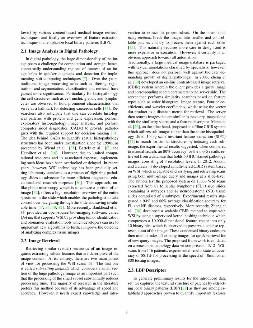
We manually selected 24 WSIs purely based on visual
distinction for non-clinical experts which means, in our se-
lection, we made conscious effort to select a subset of the
WSIs such that they clearly represent different texture pat-
terns. Fig. 1 shows the thumbnails of six samples. Fig. 2
displays a magnified portion of each WSI.
1http://www.hurondigitalpathology.com/tissuescope-le-3/
Our intention is to provide a fixed testing dataset to fa-
cilitate benchmarking but respect the design freedom of in-
dividual algorithm designer to generate his own training
dataset. To achieve this, we performed the following steps:
1. We set a fixed size of testing patches to be 1000×1000
pixels that correspond to 0.5mm ×0.5mm.
2. We ignored background pixels (patches) by setting
them to white. We performed this by analyzing
both homogeneity and gradient change of each patch
whereas a threshold was used to exclude background
patches (which are widely homogenous and do not ex-
hibit much gradient information).
3. We manually selected ni patches per WSI with i =
{1, 2, . . . , 24}. The visual patch selection aimed to ex-
tract a small number of patches that represent all dom-
inant tissue textures in each WSI (in fact, every scan
does contain multiple texture patterns).
4. Each selected patch was then removed from the scan
and saved separately as a testing patch.
5. The remaining parts of the WSI can be used to con-
struct a training dataset.
Fig. 3 demonstrate the patch selection for a sample WSI.
The scans are available online and can be downloaded 2.
The dimensions and number of testing patches for each scan
are reported in Table 1.
3.1. Accuracy Calculation
We have a total of ntot = 1, 325 patches P js that belong
to 24 sets Γs = {P is |s ∈ S, i = 1, 2 . . . , nΓs
} with s =
0, 1, 2, . . . , 23 (nΓsreported in the last column of Table 1).
Looking at the set of retrieved images R for any experiment,
the patch-to-scan accuracy ηp can be given as
ηp =
∑s∈S
|R ∩ Γs|
ntot
. (1)
As well, we calculate the whole-scan accuracy ηW as
ηW =1
24
∑
s∈S
|R ∩ Γs|
nΓs
. (2)
Hence, the total accuracy ηtotal can be defined to take into
account both patch-to-scan and whole-scan accuracies:
ηtotal = ηp × ηW. (3)
The Matlab and Python code for accuracy calculations can
also be downloaded.
2Downloading the dataset: http://kimia.uwaterloo.ca
10
Figure 1. The “Kimia Path24” Dataset: Thumbnails of six sample whole scan images. Aspect ratio has been neglected for better illustration.
4. Experiments on “Kimia Path24” Dataset
To provide preliminary results to set a benchmark line
for the proposed data set, we performed three series of re-
trieval and classification experiments: (i) Local Binary Pat-
tern (LBP), (ii) Bag of Words (BOW), and (iii) Convolu-
tional Neural Networks (CNN). The following subsections
will elaborate on every series of experiments and report the
overall accuracy of each method. Table 2 provides the re-
sults for all tested methods.
11

Figure 2. All 24 scans used to generate the Kimia Path24 dataset. The images represent approximately 20x magnification of a portion of
the whole scan images as depicted in Fig. 1.
12

Figure 3. A whole scan image (top left) and the visualization of its patch selection (top right). White squares are selected for testing. The
grey region can be used to generate training/indexing dataset. Six samples, 1000 × 1000 and grey-scaled, are displayed as examples for
testing patches extracted from the whole scan.
Figure 4. Sample for retrieval: a query patch (left image, framed) and its top three search results.
13

Table 1. Kimia Path24 dataset: Properties of each scan
Scan Index Dimensions Number of Test Patches
0 40300 × 58300 65
1 37800 × 50400 65
2 44600 × 77800 65
3 50100 × 77200 75
4 26500 × 13600 15
5 27800 × 32500 40
6 38300 × 51800 70
7 29600 × 34300 50
8 40100 × 41500 60
9 40000 × 50700 60
10 47500 × 84700 70
11 44100 × 52700 70
12 45400 × 60100 70
13 79900 × 56600 60
14 42800 × 58200 60
15 20200 × 57100 30
16 35300 × 46300 45
17 48700 × 61500 45
18 26000 × 49600 25
19 30700 × 70400 25
20 48200 × 81400 65
21 38500 × 40500 65
22 40500 × 45700 65
23 36900 × 49000 65
4.1. Experiment 1: Local Binary Patterns
For the first experiment, LBP histograms are computed
by setting several different parameters to identify the proper
windows size. In particular, the LBP is designed using
MATLAB 2016b according to [29]. After computation of
descriptors for test and training data for each configuration,
we evaluate the discriminative power of each one by k-NN
search (with k = 1) to find similar patches. Test images
with actual sizes (1000 × 1000) are fed to the LBP opera-
tor. For the training set, as discussed in the 3, we have the
option to create our training data from each scan depend-
ing on retrieval or classification method. The scans are tiled
into patches of the same size as the test patches without
any overlap. Then we remove patches with a homogeneity
of more than 99%. Using this configuration, we extracted
27, 055 training images which are compared against each
test patch for similarity measurement. Non-rotational ver-
sions of uniform LBP [29] of radii 1, 2 and 3 with 8,16 and
24 neighbors, respectively, are applied to create a histogram
of length 59, 243 and 555. Varying radius helps LBP to cap-
ture the texture in different scales, which could be a signif-
icant research question in WSI processing [13]. As shown
in Table 2, a longer radius contributes to an increase in both
accuracy (2%-3% at most) and descriptor length.
4.2. Experiment 2: BagofWords Approach
For the second experiment, a dictionary learning ap-
proach, i.e., Bag-of-Words (BOW), was designed by min-
imizing the error of the training samples to build the over-
complete dictionary (i.e., the codebook) [18, 25]. The de-
sign of the BOW approach was conducted according to [20].
The frequency of occurrence of the word histogram can be
assigned to describe the input based on the trained dictio-
nary. To train the pathology patch dictionary, two descrip-
tors are used: the raw pixels and the LBP of the raw pix-
els in each neighborhood. Before extracting the descrip-
tors, 300 patches are selected randomly from all available
patches such that their gradient is larger than the average
gradient value of all patches for each scan. To accelerate
the dictionary training, all 7,200 = 24 × 300 patches are
down-sampled to 500×500 and meshed into 16×16 grids
without overlap. Raw pixel descriptors and LBP features
are extracted from these sub-patches. The extracted descrip-
tors are used for training the dictionary whose size is set to
800. The word-frequency histogram of each patch is then
encoded using the learned dictionary. Finally, the word his-
togram with its corresponding scan labels is fed to SVM
classification with histogram intersection kernel [9]. From
the obtained results, depicted in Table 2, we can see that us-
ing raw pixels or LBP features result in roughly the same
accuracy. However, LBP was observed to be much quicker
to train and computationally less expensive as compared to
raw pixels.
4.3. Experiment 3: Convolutional Neural Network
For the last experiment, we used two deep convolution
neural networks (CNN), architecturally and conceptually
inspired by Alexnet [19] and VGG16 [33]. The first net-
work, CNN1, is trained from scratch using end-to-end train-
ing with limited pre-processing. For each of the 24 scans,
patches are extracted with 40% overlap, and 99% homo-
geneity threshold, further filtered with top 60% of gradient
values and re-sized to 128 × 128 using bicubic interpola-
tion. This results in a total of 40,513 patches for training.
The CNN consists of 3 convolutional layers with 3 × 3 ker-
nels, each with 2× 2 max-pooling with 64, 128, and 256
filters, respectively. The output from the last convolution
layer is fed into a fully-connected layer with 1,024 neu-
rons and subsequently to 24 units with softmax activation
for classification. Other than the last layer, all other lay-
ers in the network use ReLu as the activation function. The
Adam optimizer is used with a learning rate of 0.001 and the
categorical cross-entropy is used as the loss function. The
network achieves the highest accuracy of ηtotal = 41.80%
for the proposed dataset.
In another experiment, a slightly different architecture,
CNN2 was considered for classifying the images. A shal-
low structure of three blocks with 16, 32, and 64 filters
14

Table 2. Preliminary results for the Kimia Path24 dataset. LBP
uses different distance measures (L1, L2 and χ2) in different con-
figurations (n, r) for n neighbours and radius r. Best results for
ηp, ηW and ηtotal are highlighted in bold.
Method ηp ηW ηtotal
LBPu(8,1), χ
2 62.49 58.92 36.82
LBPu(8,1), L1 61.13 57.50 35.15
LBPu(8,1), L2 56.45 52.95 29.89
LBPu(16,2), χ
2 63.62 59.51 37.86
LBPu(16,2), L1 62.26 58.19 36.23
LBPu(16,2), L2 55.77 52.12 29.07
LBPu(24,3), χ
2 64.67 61.08 39.50
LBPu(24,3), L1 66.11 62.52 41.33
LBPu(24,3), L2 59.01 55.94 33.01
BOWRAW 64.98 61.02 39.65
BOWLBP 64.68 59.33 38.37
CNN1 64.98 64.75 41.80
CNN2 64.98 61.92 40.24
was investigated. The high-level extracted features from the
last convolutional layer are passed to one fully connected
layer with 625 neurons, followed by a softmax classifier
at the top. Our experiments showed that applying 35%
dropout with L2 norm regularization technique achieves
around 40.24% accuracy.
4.4. Analysis and Discussion
The data set we are proposing may be regarded easy be-
cause we are trying to match patches that come from the
same scan/patient. However, as the results demonstrate, this
is clearly not the case. The BoW approach was able to pro-
vide a much more compact representation (codebook). Be-
sides, the storage requirements are quite low. However, the
geometric and spatial relations between words are generally
neglected. Apparently, the outliers in the training data make
it fail to perform properly. CNN achieved the best result
of 41.80% followed by LBP with an accuracy of 41.33%.
CNN, most likely, can still improve if a larger training set
is extracted from the scans. And as for LBP, perhaps using
some classifier may increase the accuracy. One should bear
in mind that LBP did in fact process the images in their orig-
inal dimensions whereas CNNs required substantial down-
sampling. Taking into account the training complexity, one
may prefer LBP over CNNs for the former is intrinsically
simple and fast. As well, LBP has been designed to deal
with textures at the spatial level.
5. Summary
In this paper, we put forward Kimia Path24, a new data
set for retrieval and classification of digital pathology scans.
We selected 24 scans from a large pool of scans through vi-
sual inspection. The criterion was to select texturally differ-
ent images. Hence, the proposed data set is rather a com-
puter vision data set (as in contrast to a pathological data
set) because visual attention has been spent on the diversity
of patterns and not on anatomies and malignancies. The
task, hence, is whether machine-learning algorithms can
discriminate among diverse patterns. To start a baseline, we
applied LBP, the dictionary approach and CNNs to classify
patches. The results show that the task is apparently quite
difficult.
The data set can be downloaded from authors’ website:
http://kimia.uwaterloo.ca
References
[1] H. C. Akakin and M. N. Gurcan. Content-based micro-
scopic image retrieval system for multi-image queries. IEEE
transactions on information technology in biomedicine,
16(4):758–769, 2012. 2
[2] S. Al-Janabi, A. Huisman, and P. J. Van Diest. Digital pathol-
ogy: current status and future perspectives. Histopathology,
61(1):1–9, 2012. 1
[3] M. Babaie, H. R. Tizhoosh, S. Zhu, and M. E. Shiri. Retriev-
ing similar x-ray images from big image data using radon
barcodes with single projections. In Proceedings of the 6th
International Conference on Pattern Recognition Applica-
tions and Methods, pages 557–566, 2017. 3
[4] P. Bankhead, M. B. Loughrey, J. A. Fernandez, Y. Dom-
browski, D. G. McArt, P. D. Dunne, S. McQuaid, R. T. Gray,
L. J. Murray, H. G. Coleman, et al. Qupath: Open source
software for digital pathology image analysis. bioRxiv, page
099796, 2017. 2
[5] J. Barker, A. Hoogi, A. Depeursinge, and D. L. Rubin. Auto-
mated classification of brain tumor type in whole-slide digi-
tal pathology images using local representative tiles. Medical
image analysis, 30:60–71, 2016. 2
[6] P. Bartels, D. Thompson, M. Bibbo, and J. Weber. Bayesian
belief networks in quantitative histopathology. Analytical
and quantitative cytology and histology/the International
Academy of Cytology [and] American Society of Cytology,
14(6):459–473, 1992. 2
[7] J. C. Caicedo, F. A. Gonzalez, and E. Romero. Content-
based histopathology image retrieval using a kernel-based
semantic annotation framework. Journal of biomedical in-
formatics, 44(4):519–528, 2011. 2
[8] A. E. Carpenter, L. Kamentsky, and K. W. Eliceiri. A call
for bioimaging software usability. Nature methods, 9(7):666,
2012. 1
[9] C.-C. Chang and C.-J. Lin. LIBSVM: A library for support
vector machines. ACM Transactions on Intelligent Systems
and Technology, 2:1–27, 2011. 7
[10] V. Della Mea, N. Bortolotti, and C. Beltrami. eslide suite: an
open source software system for whole slide imaging. Jour-
nal of clinical pathology, 62(8):749–751, 2009. 2
[11] M. Y. Gabril and G. Yousef. Informatics for practicing
anatomical pathologists: marking a new era in pathology
practice. Mod Pathol, 23(3):349–358, 2010. 1
15

[12] F. Ghaznavi, A. Evans, A. Madabhushi, and M. Feldman.
Digital imaging in pathology: whole-slide imaging and be-
yond. Annual Review of Pathology: Mechanisms of Disease,
8:331–359, 2013. 1, 2
[13] J. R. Gilbertson, J. Ho, L. Anthony, D. M. Jukic, Y. Yagi,
and A. V. Parwani. Primary histologic diagnosis using auto-
mated whole slide imaging: a validation study. BMC clinical
pathology, 6(1):4, 2006. 7
[14] M. N. Gurcan, L. E. Boucheron, A. Can, A. Madabhushi,
N. M. Rajpoot, and B. Yener. Histopathological image anal-
ysis: A review. IEEE reviews in biomedical engineering,
2:147–171, 2009. 2
[15] D. A. Gutman, J. Cobb, D. Somanna, Y. Park, F. Wang,
T. Kurc, J. H. Saltz, D. J. Brat, L. A. Cooper, and J. Kong.
Cancer digital slide archive: an informatics resource to sup-
port integrated in silico analysis of tcga pathology data.
Journal of the American Medical Informatics Association,
20(6):1091–1098, 2013. 2
[16] P. Hamilton, N. Anderson, P. Bartels, and D. Thompson. Ex-
pert system support using bayesian belief networks in the
diagnosis of fine needle aspiration biopsy specimens of the
breast. J. of Clinical Pathology, 47(4):329–336, 1994. 2
[17] J. Ho, A. V. Parwani, D. M. Jukic, Y. Yagi, L. Anthony,
and J. R. Gilbertson. Use of whole slide imaging in surgi-
cal pathology quality assurance: design and pilot validation
studies. Human pathology, 37(3):322–331, 2006. 1, 2
[18] T. Joachims. Text categorization with support vector ma-
chines: Learning with many relevant features. Machine
learning: ECML-98, pages 137–142, 1998. 3, 7
[19] A. Krizhevsky, I. Sutskever, and G. E. Hinton. Imagenet
classification with deep convolutional neural networks. In
Advances in neural information processing systems, pages
1097–1105, 2012. 7
[20] S. Lazebnik, C. Schmid, and J. Ponce. Beyond bags of
features: Spatial pyramid matching for recognizing natural
scene categories. In Computer vision and pattern recogni-
tion, 2006 IEEE computer society conference on, volume 2,
pages 2169–2178. IEEE, 2006. 7
[21] Y. LeCun, L. Bottou, Y. Bengio, and P. Haffner. Gradient-
based learning applied to document recognition. Proceed-
ings of the IEEE, 86(11):2278–2324, 1998. 3
[22] D. G. Lowe. Object recognition from local scale-invariant
features. In Computer vision, 1999. The proceedings of the
seventh IEEE international conference on, volume 2, pages
1150–1157. Ieee, 1999. 2
[23] A. Madabhushi and G. Lee. Image analysis and machine
learning in digital pathology: Challenges and opportunities.
Medical Image Analysis, 33:170–175, 2017. 1
[24] K. Masood and N. Rajpoot. Texture based classification of
hyperspectral colon biopsy samples using clbp. In IEEE In-
ternational Symposium on Biomedical Imaging, pages 1011–
1014, 2009. 3
[25] A. McCallum, K. Nigam, et al. A comparison of event mod-
els for naive bayes text classification. In AAAI-98 workshop
on learning for text categorization, volume 752, pages 41–
48. Citeseer, 1998. 3, 7
[26] N. Mehta, A. Raja’S, and V. Chaudhary. Content based sub-
image retrieval system for high resolution pathology images
using salient interest points. In IEEE International Confer-
ence of the Engineering in Medicine and Biology Society,
pages 3719–3722, 2009. 2
[27] L. Nanni, A. Lumini, and S. Brahnam. Local binary patterns
variants as texture descriptors for medical image analysis.
Artificial intelligence in medicine, 49(2):117–125, 2010. 3
[28] T. Ojala, M. Pietikainen, and D. Harwood. Performance eval-
uation of texture measures with classification based on kull-
back discrimination of distributions. In Proceedings of the
12th IAPR International Conference on Computer Vision &
Image Processing, volume 1, pages 582–585, 1994. 2
[29] T. Ojala, M. Pietikainen, and T. Maenpaa. Multiresolution
gray-scale and rotation invariant texture classification with
local binary patterns. IEEE Transactions on pattern analysis
and machine intelligence, 24(7):971–987, 2002. 7
[30] L. Pantanowitz, P. N. Valenstein, A. J. Evans, K. J. Kaplan,
J. D. Pfeifer, D. C. Wilbur, L. C. Collins, T. J. Colgan, et al.
Review of the current state of whole slide imaging in pathol-
ogy. Journal of pathology informatics, 2(1):36, 2011. 2
[31] Y. A. Reyad, M. A. Berbar, and M. Hussain. Compari-
son of statistical, lbp, and multi-resolution analysis features
for breast mass classification. Journal of medical systems,
38(9):100, 2014. 3
[32] O. Sertel, J. Kong, H. Shimada, U. Catalyurek, J. H. Saltz,
and M. N. Gurcan. Computer-aided prognosis of neuroblas-
toma on whole-slide images: Classification of stromal devel-
opment. Pattern recognition, 42(6):1093–1103, 2009. 3
[33] K. Simonyan and A. Zisserman. Very deep convolutional
networks for large-scale image recognition. arXiv preprint
arXiv:1409.1556, 2014. 7
[34] A. Tashk, M. S. Helfroush, H. Danyali, and M. Akbarzadeh.
An automatic mitosis detection method for breast cancer
histopathology slide images based on objective and pixel-
wise textural features classification. In Conference on Infor-
mation and Knowledge Technology, pages 406–410, 2013.
3
[35] K. L. Weind, C. F. Maier, B. K. Rutt, and M. Moussa. Inva-
sive carcinomas and fibroadenomas of the breast: compar-
ison of microvessel distributions–implications for imaging
modalities. Radiology, 208(2):477–483, 1998. 2
[36] R. S. Weinstein, A. R. Graham, L. C. Richter, G. P. Barker,
E. A. Krupinski, A. M. Lopez, K. A. Erps, A. K. Bhat-
tacharyya, Y. Yagi, and J. R. Gilbertson. Overview of
telepathology, virtual microscopy, and whole slide imaging:
prospects for the future. Human pathology, 40(8):1057–
1069, 2009. 2
[37] S. Williams, W. H. Henricks, M. J. Becich, M. Toscano,
and A. B. Carter. Telepathology for patient care: what am
i getting myself into? Advances in anatomic pathology,
17(2):130–149, 2010. 2
[38] X. Zhang, W. Liu, M. Dundar, S. Badve, and S. Zhang.
Towards large-scale histopathological image analysis:
Hashing-based image retrieval. IEEE Transactions on Med-
ical Imaging, 34(2):496–506, 2015. 2
[39] L. Zheng, A. W. Wetzel, J. Gilbertson, and M. J. Becich.
Design and analysis of a content-based pathology image re-
trieval system. IEEE Transactions on Information Technol-
ogy in Biomedicine, 7(4):249–255, 2003. 2
16