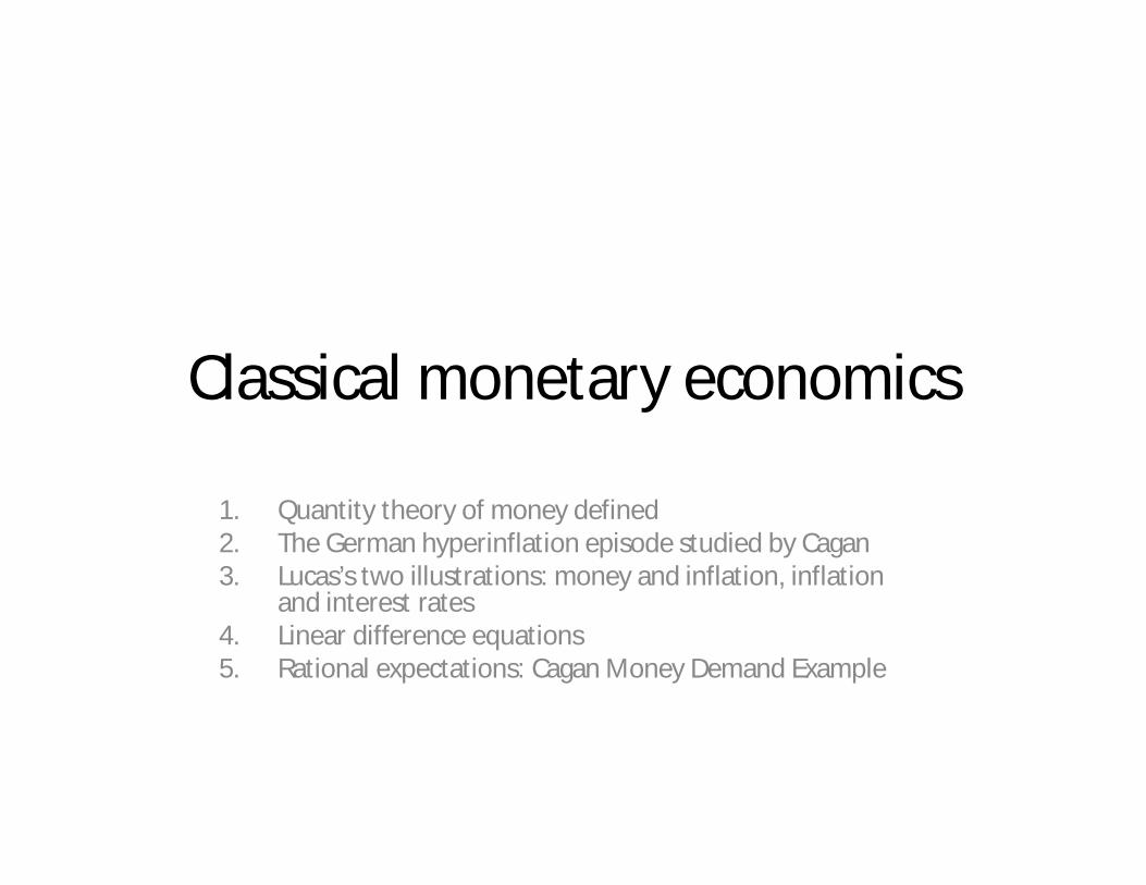
Classical monetary economics

1. Quantity theory of money defined2. The German hyperinflation episode studied by Cagan3. Lucas’s two illustrations: money and inflation, inflation

and interest rates4. Linear difference equations5. Rational expectations: Cagan Money Demand Example

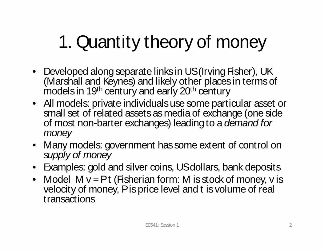
1. Quantity theory of money• Developed along separate links in US (Irving Fisher), UK

(Marshall and Keynes) and likely other places in terms of models in 19th century and early 20th century

• All models: private individuals use some particular asset or small set of related assets as media of exchange (one side of most non-barter exchanges) leading to a demand for money

• Many models: government has some extent of control on supply of money

• Examples: gold and silver coins, US dollars, bank deposits• Model M v = P t (Fisherian form: M is stock of money, v is

velocity of money, P is price level and t is volume of real transactions

EC541: Session 1 2

Key proposition

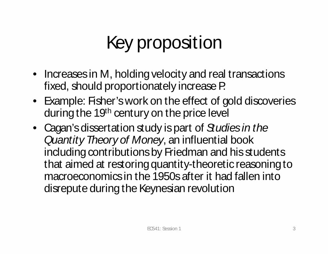
• Increases in M, holding velocity and real transactions fixed, should proportionately increase P.

• Example: Fisher’s work on the effect of gold discoveries during the 19th century on the price level

• Cagan’s dissertation study is part of Studies in the Quantity Theory of Money, an influential book including contributions by Friedman and his students that aimed at restoring quantity-theoretic reasoning to macroeconomics in the 1950s after it had fallen into disrepute during the Keynesian revolution

EC541: Session 1 3

Often associated with

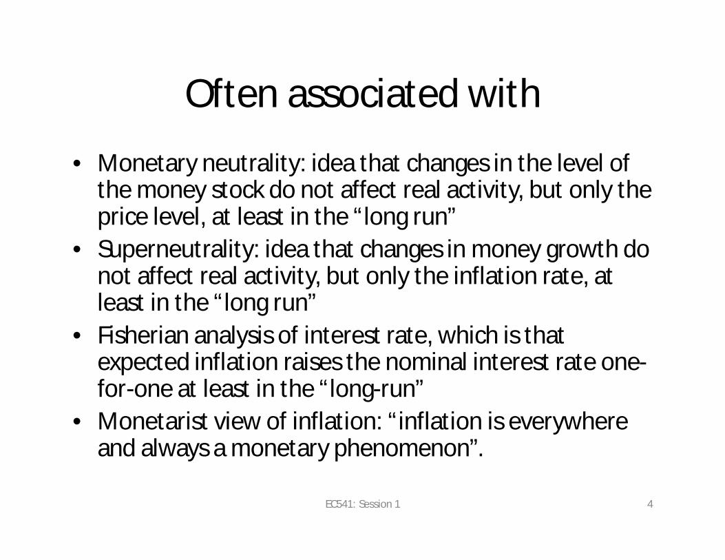
• Monetary neutrality: idea that changes in the level of the money stock do not affect real activity, but only the price level, at least in the “long run”

• Superneutrality: idea that changes in money growth do not affect real activity, but only the inflation rate, at least in the “long run”

• Fisherian analysis of interest rate, which is that expected inflation raises the nominal interest rate one-for-one at least in the “long-run”

• Monetarist view of inflation: “inflation is everywhere and always a monetary phenomenon”.

EC541: Session 1 4

Cagan

• The strategy of Cagan was to look at a series of historical episodes – hyperinflation episodes, which he defines as involving inflation at more than 50% per month -- in which high rates of money growth made it plausible that all other factors would be not too important

• But, in this setting, a simple QT approach with v and t constant was not sufficient. High expected inflation caused substitution away from money holding

EC541: Session 1 5

2. One of Cagan’s hyperinflations:Germany 1920-1923

• Weimar republic issued a large number of paper marks

• Inability or unwillingness to directly tax the economy in the aftermath of WWI led to use of “inflation tax”.

• Historical period is nicely summarized in Wikipedia entry (although one must be careful with this source more generally): http://en.wikipedia.org/wiki/Inflation_in_the_Weimar_Republic

EC541: Session 1 6

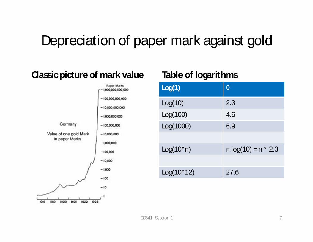
Depreciation of paper mark against gold

Classic picture of mark value Table of logarithmsLog(1) 0

Log(10) 2.3

Log(100) 4.6

Log(1000) 6.9

Log(10^n) n log(10) = n * 2.3

Log(10^12) 27.6

EC541: Session 1 7

Cagan’s data on money and price level

1920.5 1921 1921.5 1922 1922.5 1923 1923.5 1924-5

0

5

10

15

20

25

30

time

log(

P) a

nd lo

g(M

)

MoneyPrice Level

EC541: Session 1 8

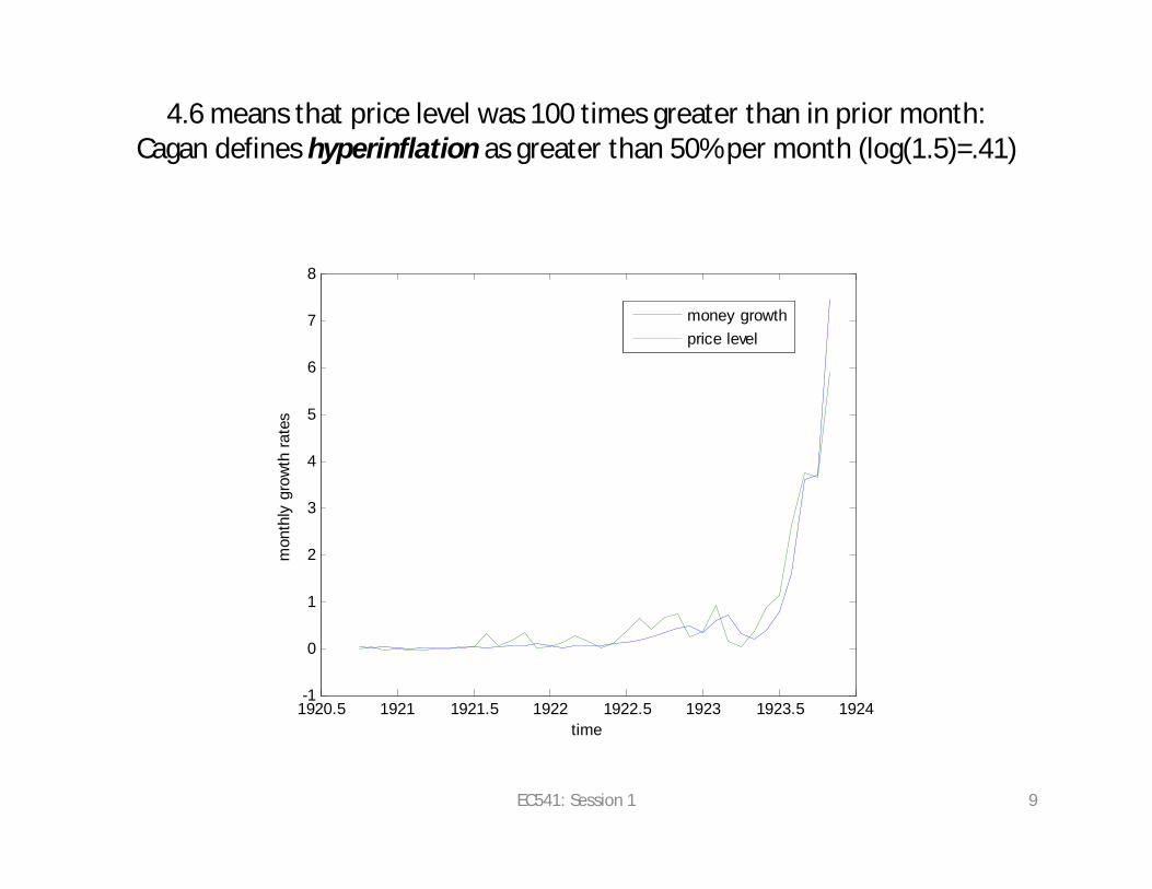
4.6 means that price level was 100 times greater than in prior month:Cagan defines hyperinflation as greater than 50% per month (log(1.5)=.41)

1920.5 1921 1921.5 1922 1922.5 1923 1923.5 1924-1

0

1

2

3

4

5

6

7

8

time

mon

thly

gro

wth

rate

s

money growthprice level

EC541: Session 1 9

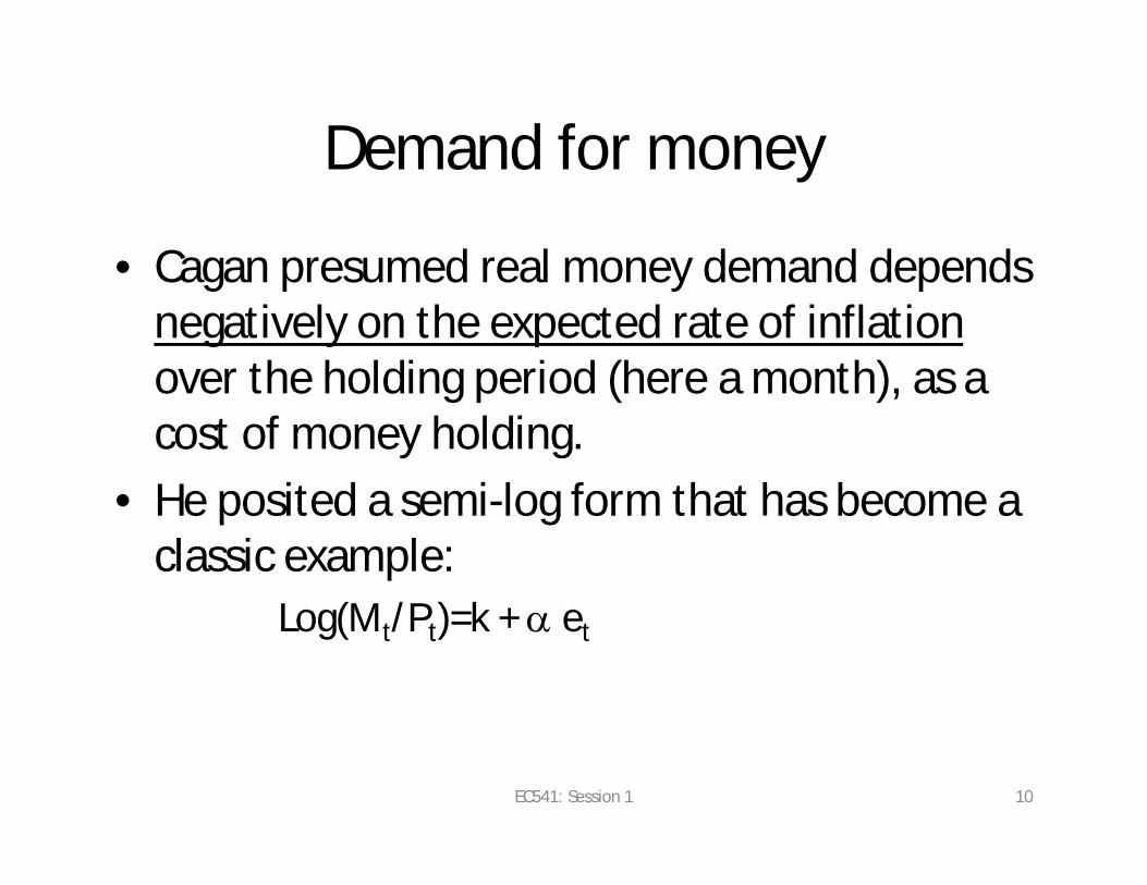
Demand for money

• Cagan presumed real money demand depends negatively on the expected rate of inflation over the holding period (here a month), as a cost of money holding.

• He posited a semi-log form that has become a classic example:

Log(Mt/Pt)=k + a et

EC541: Session 1 10

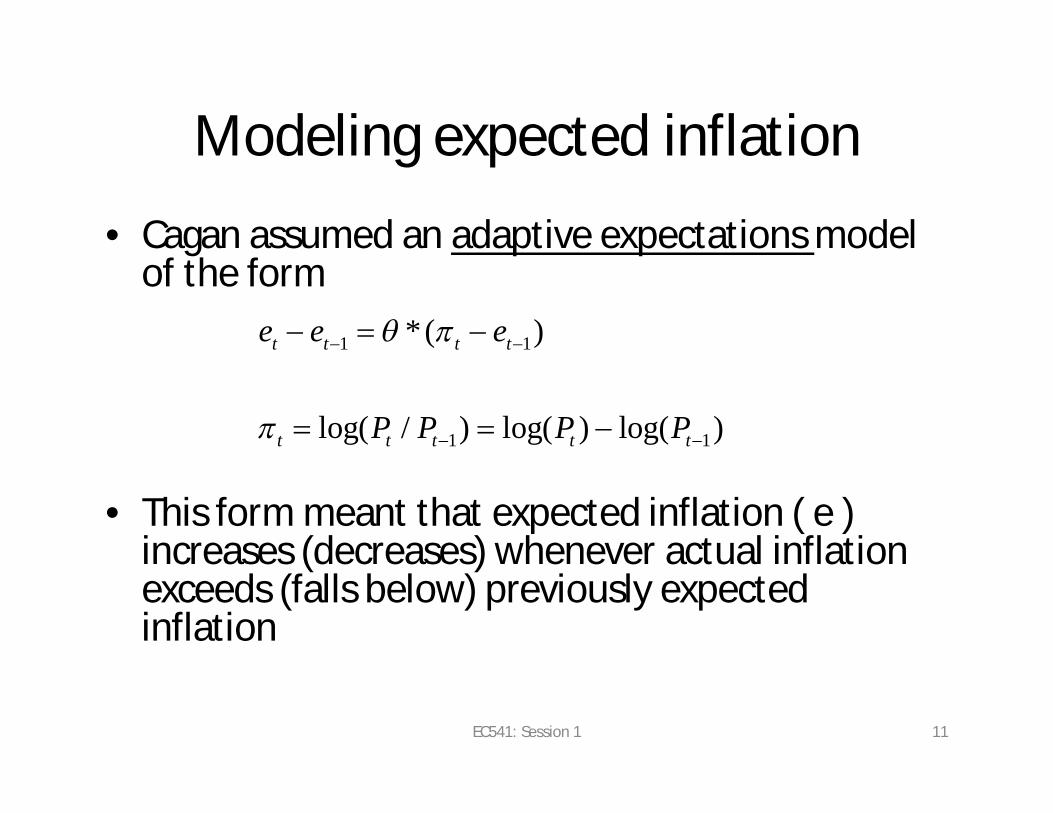
Modeling expected inflation

• Cagan assumed an adaptive expectations model of the form

• This form meant that expected inflation ( e ) increases (decreases) whenever actual inflation exceeds (falls below) previously expected inflation

1 1

1 1

*( )

log( / ) log( ) log( )

t t t t

t t t t t

e e e

P P P P

EC541: Session 1 11

Two views of Cagan’sGerman regression

1. Visualize links between two series over June 1920 through end of 1922

2. Estimate OLS specification (we do it with fixed theta (q), while Cagan estimated k,a for each fixed q and then chose best fit)

EC541: Session 1 12

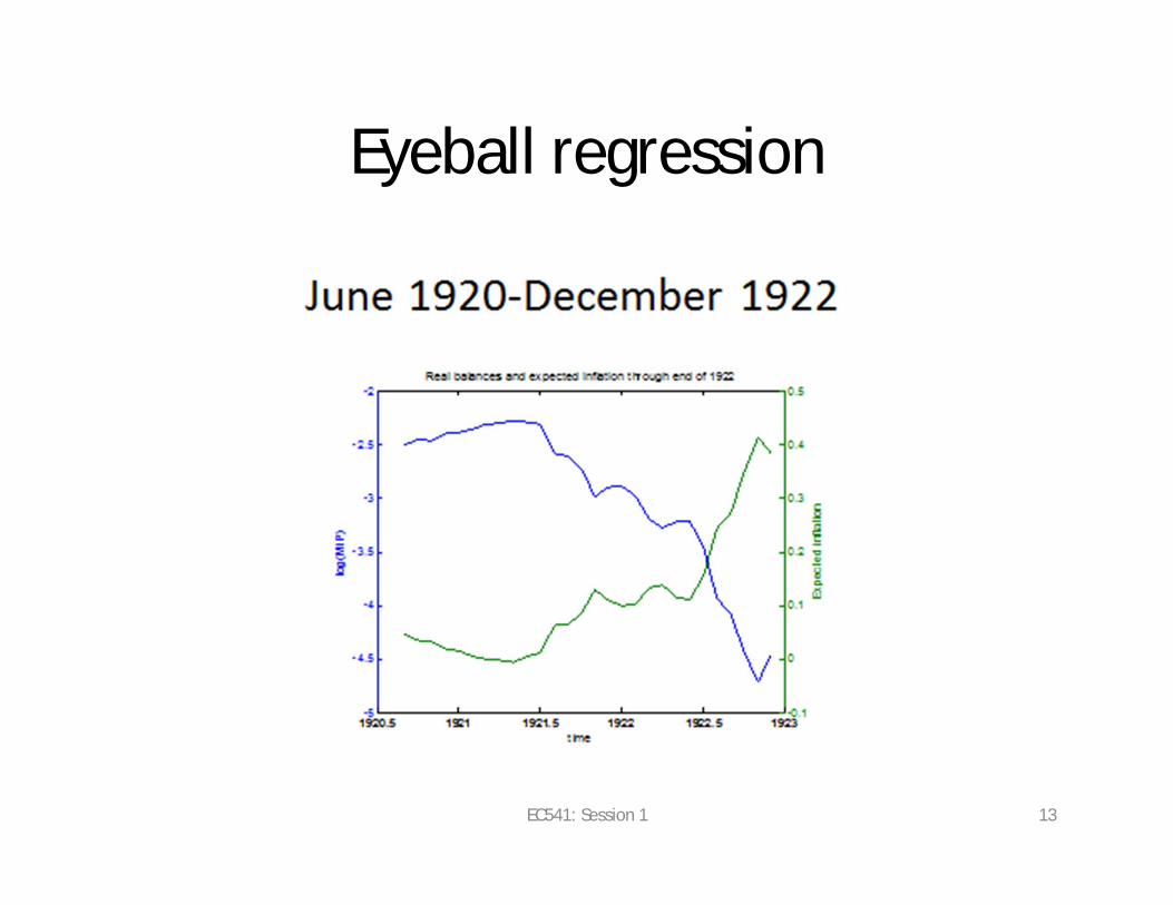
Eyeball regression

EC541: Session 1 13

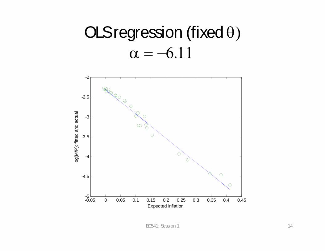
OLS regression (fixed q)a 6.11

-0.05 0 0.05 0.1 0.15 0.2 0.25 0.3 0.35 0.4 0.45-5

-4.5

-4

-3.5

-3

-2.5

-2

Expected Inflation

log(

M/P

); fit

ted

and

actu

al

EC541: Session 1 14

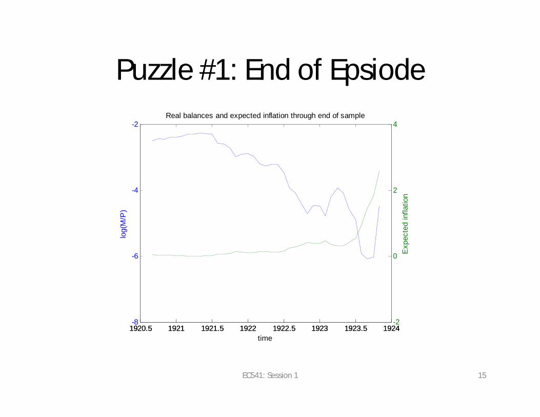
Puzzle #1: End of Epsiode

1920.5 1921 1921.5 1922 1922.5 1923 1923.5 1924-8

-6

-4

-2lo

g(M

/P)

time

Real balances and expected inflation through end of sample

1920.5 1921 1921.5 1922 1922.5 1923 1923.5 1924-2

0

2

4

Exp

ecte

d in

flatio

n

EC541: Session 1 15

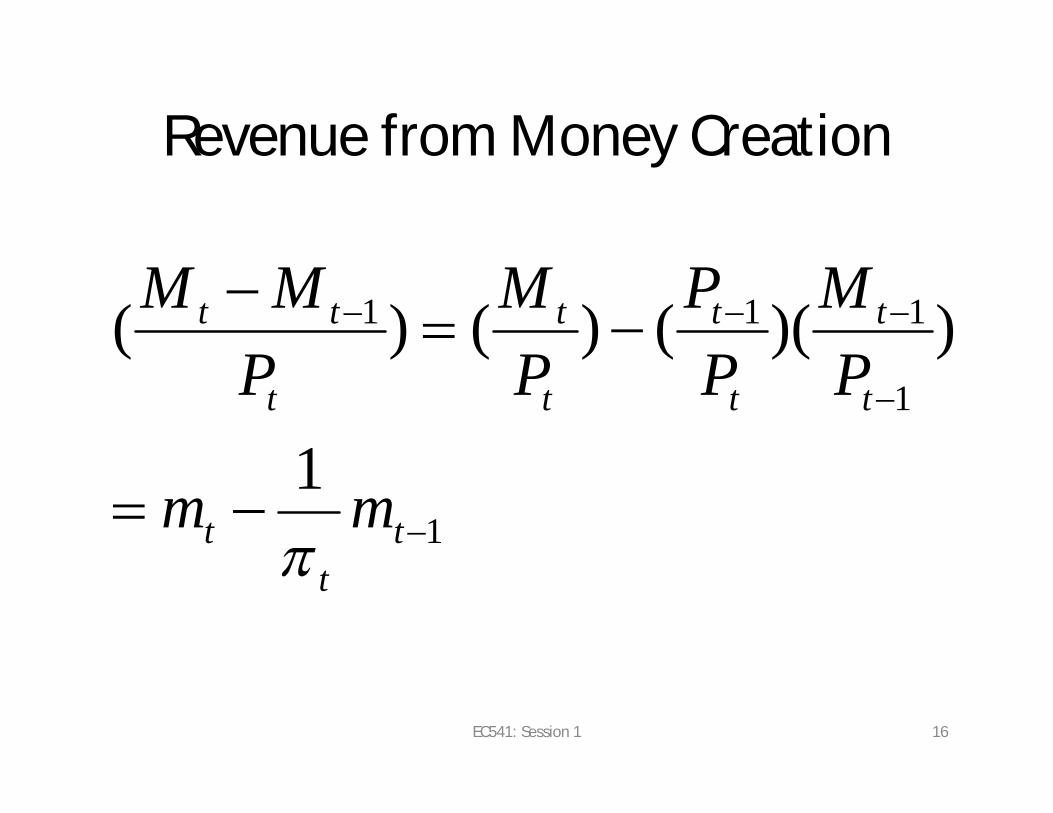
Revenue from Money Creation

1

1

111

1

))(()()(

tt

t

t

t

t

t

t

t

t

tt

mm

PM

PP

PM

PMM

EC541: Session 1 16

Revenue from money creation

• Inflation tax: if Pt = 10Pt-1 then 90% of pre-existing cash balances have been taxed away (p=10, 1/p = 1/10)

• Amount of revenue depends on:– Change in nominal money divided by price level– New real balances issued less value of prior period

real balances

EC541: Session 1 17

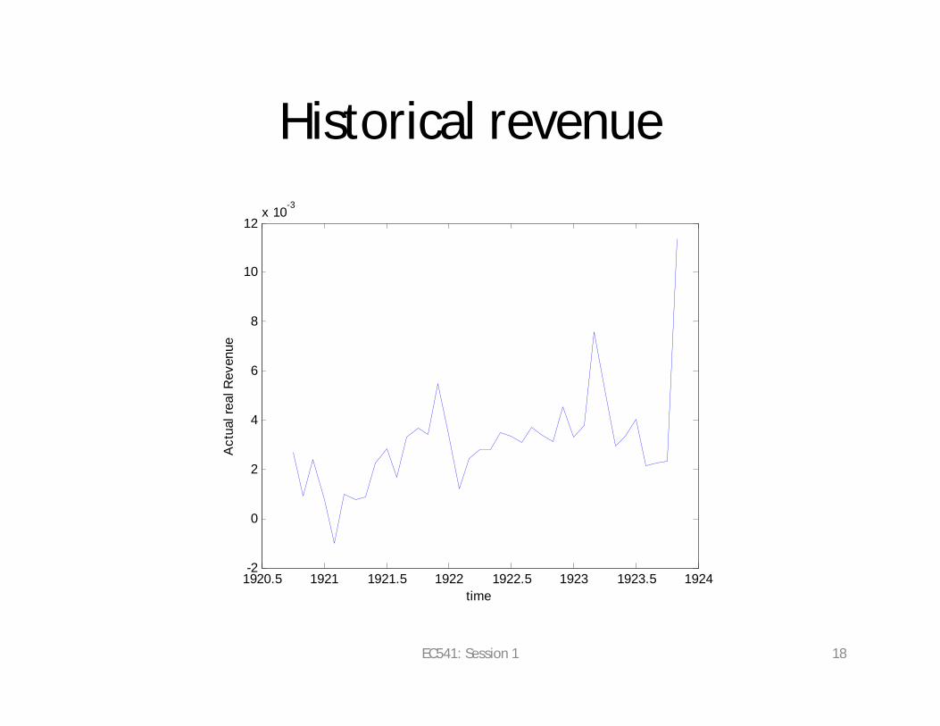
Historical revenue

1920.5 1921 1921.5 1922 1922.5 1923 1923.5 1924-2

0

2

4

6

8

10

12x 10

-3

time

Act

ual r

eal R

even

ue

EC541: Session 1 18

Qualifications

• Germany had a mixed money system– Pure paper money– Bank deposits

• Deposits can be interest bearing• Depreciation of deposits shifts revenue to

banks not to government (but to government if banks required to hold low interest government bonds)

EC541: Session 1 19

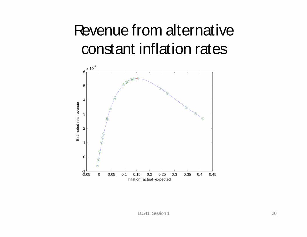
Revenue from alternative constant inflation rates

-0.05 0 0.05 0.1 0.15 0.2 0.25 0.3 0.35 0.4 0.45-1

0

1

2

3

4

5

6x 10

-3

Inflation: actual=expected

Est

imat

ed re

al re

venu

e

EC541: Session 1 20

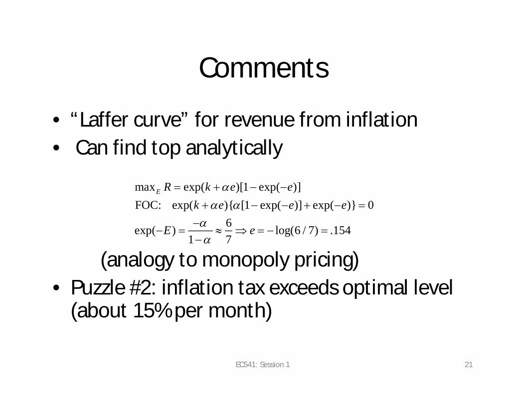
Comments

• “Laffer curve” for revenue from inflation• Can find top analytically

(analogy to monopoly pricing)• Puzzle #2: inflation tax exceeds optimal level

(about 15% per month)

max exp( )[1 exp( )]FOC: exp( ){ [1 exp( )] exp( )} 0

6exp( ) log(6 / 7) .1541 7

E R k e ek e e e

E e

EC541: Session 1 21

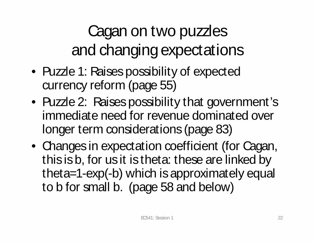
Cagan on two puzzles and changing expectations

• Puzzle 1: Raises possibility of expected currency reform (page 55)

• Puzzle 2: Raises possibility that government’s immediate need for revenue dominated over longer term considerations (page 83)

• Changes in expectation coefficient (for Cagan, this is b, for us it is theta: these are linked by theta=1-exp(-b) which is approximately equal to b for small b. (page 58 and below)

EC541: Session 1 22

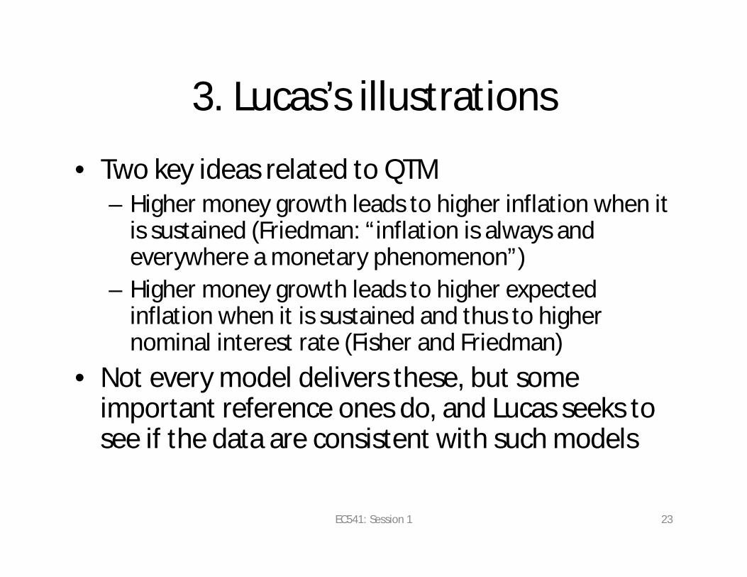
3. Lucas’s illustrations

• Two key ideas related to QTM– Higher money growth leads to higher inflation when it

is sustained (Friedman: “inflation is always and everywhere a monetary phenomenon”)

– Higher money growth leads to higher expected inflation when it is sustained and thus to higher nominal interest rate (Fisher and Friedman)

• Not every model delivers these, but some important reference ones do, and Lucas seeks to see if the data are consistent with such models

EC541: Session 1 23

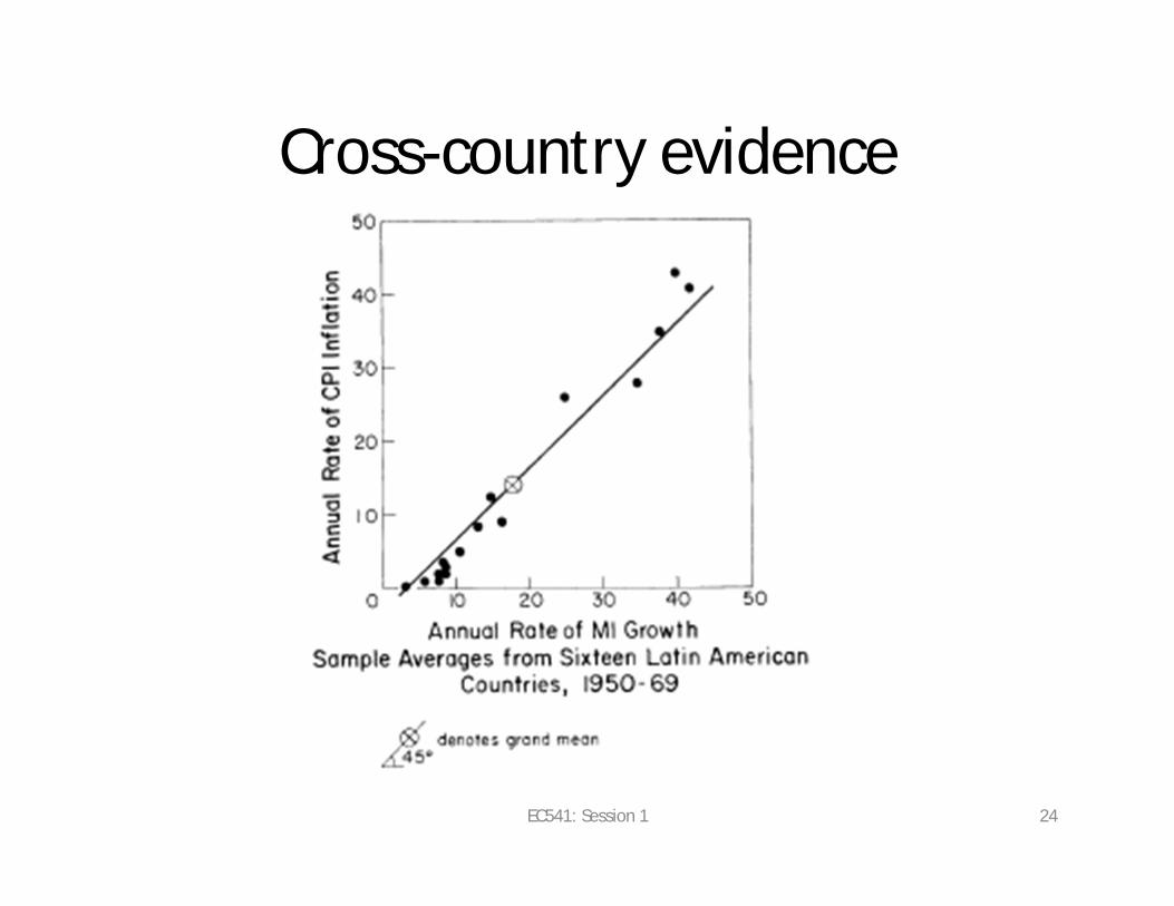
Cross-country evidence

EC541: Session 1 24

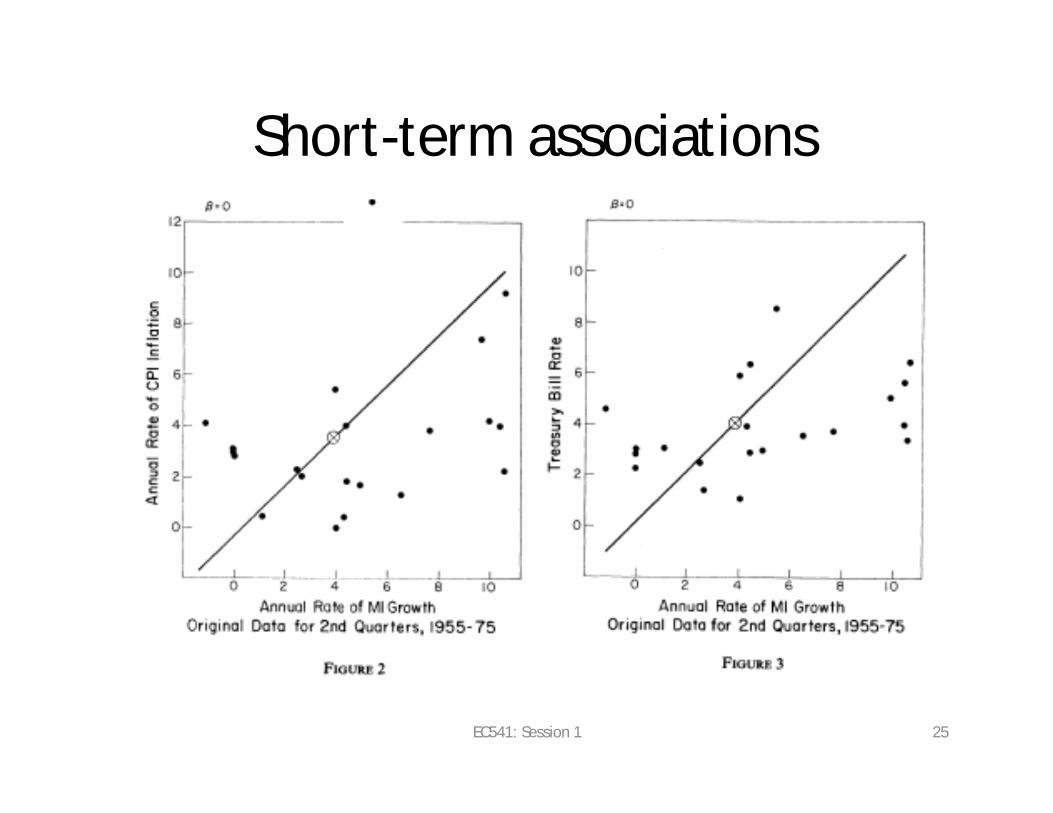
Short-term associations

EC541: Session 1 25

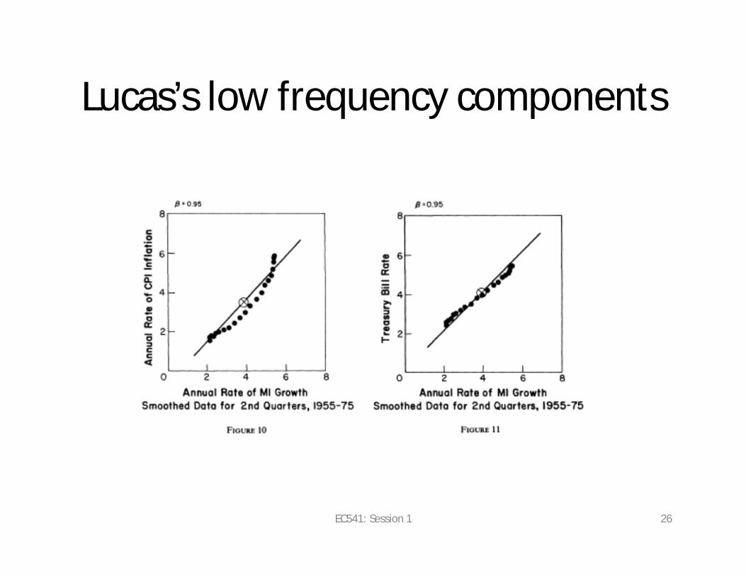
Lucas’s low frequency components

EC541: Session 1 26

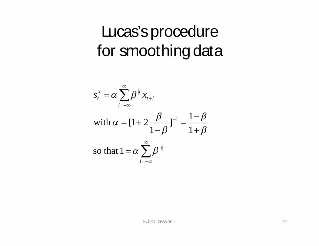
Lucas’s procedure for smoothing data

EC541: Session 1 27

i

i

iit

ixt xs

1 that so

11]

121[with

||

1

||

Why manipulate data using such a procedure?

• Highlighting “low frequency” or “trend” component because theory is partial (e.g., does not include short-run departures from neutrality or changes in real interest rate)

• Other procedures have been developed for this purpose (see laboratory work with Eviewsand self-guided work with MATLAB)

EC541: Session 1 28

Other related approaches

• Elimination of seasonals and other “high frequency” parts of series via smoothing

• Year-over-year changes to highlight recent developments

• Detrending: (x – s) in Lucas’s setting• Detrending plus smoothing to focus on

“business cycle components”

EC541: Session 1 29

4. Difference Equations

• A common element of the Cagan and Lucas studies is that they are concerned with dynamic elements

• In discrete time, this involves analysis of difference equations

• Systems of linear difference equations are used a lot because they are easy to solve and manipulate

• These are also used in analysis of rational expectations models, for the same reason.

EC541: Session 1 30

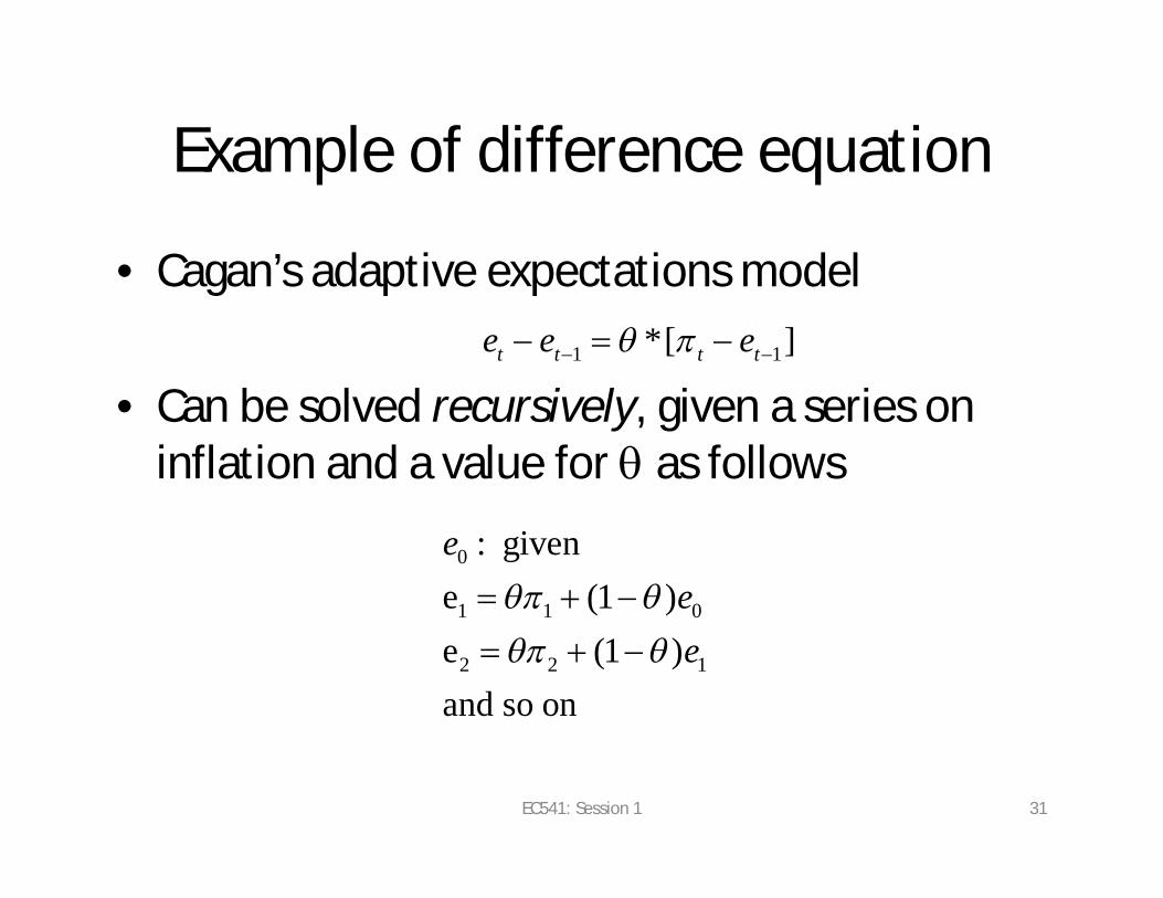
Example of difference equation

• Cagan’s adaptive expectations model

• Can be solved recursively, given a series on inflation and a value for q as follows

EC541: Session 1 31

1 1*[ ]t t t te e e

0

1 1 0

2 2 1

: givene (1 )e (1 )and so on

eee

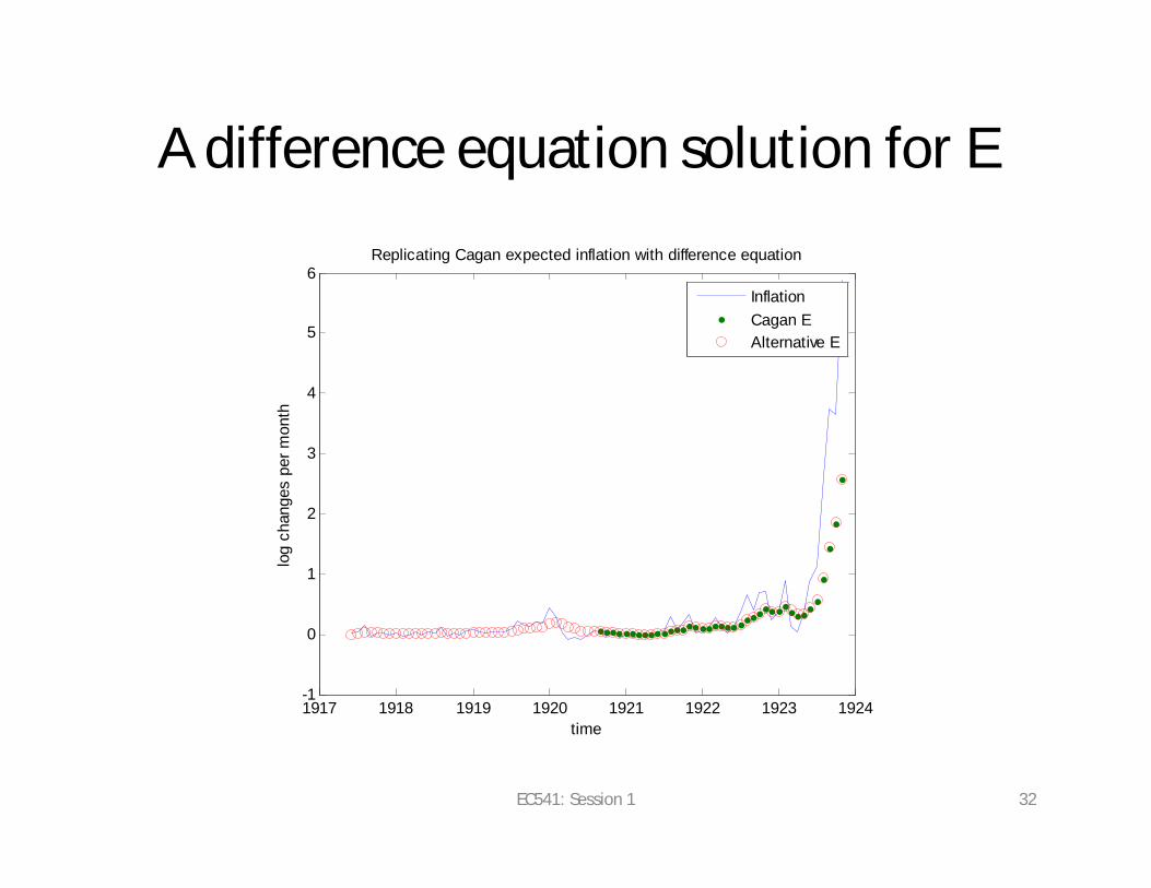
A difference equation solution for E

1917 1918 1919 1920 1921 1922 1923 1924-1

0

1

2

3

4

5

6Replicating Cagan expected inflation with difference equation

time

log

chan

ges

per m

onth

InflationCagan EAlternative E

EC541: Session 1 32

Uses of difference equations in class

• Forecasting (difference equations with shocks are called autoregressions and if they involve a vector of variables they are called vector autoregressions)

• Solutions of linear rational expectations models

• Linear approximation solutions of nonlinear RE models

• Other approximate solutions of RE models

EC541: Session 1 33

Coverage

• Not really core material of this class (you should have picked up this up in macro class EC502)

• But we’ll try to help you with aspects of this material, so that you can effectively access course elements and so that you can benefit from lab sessions

• Some self-guided study materials will be provided, which are associated with particular lectures. This lecture’s material is called difeq.pdf

EC541: Session 1 34

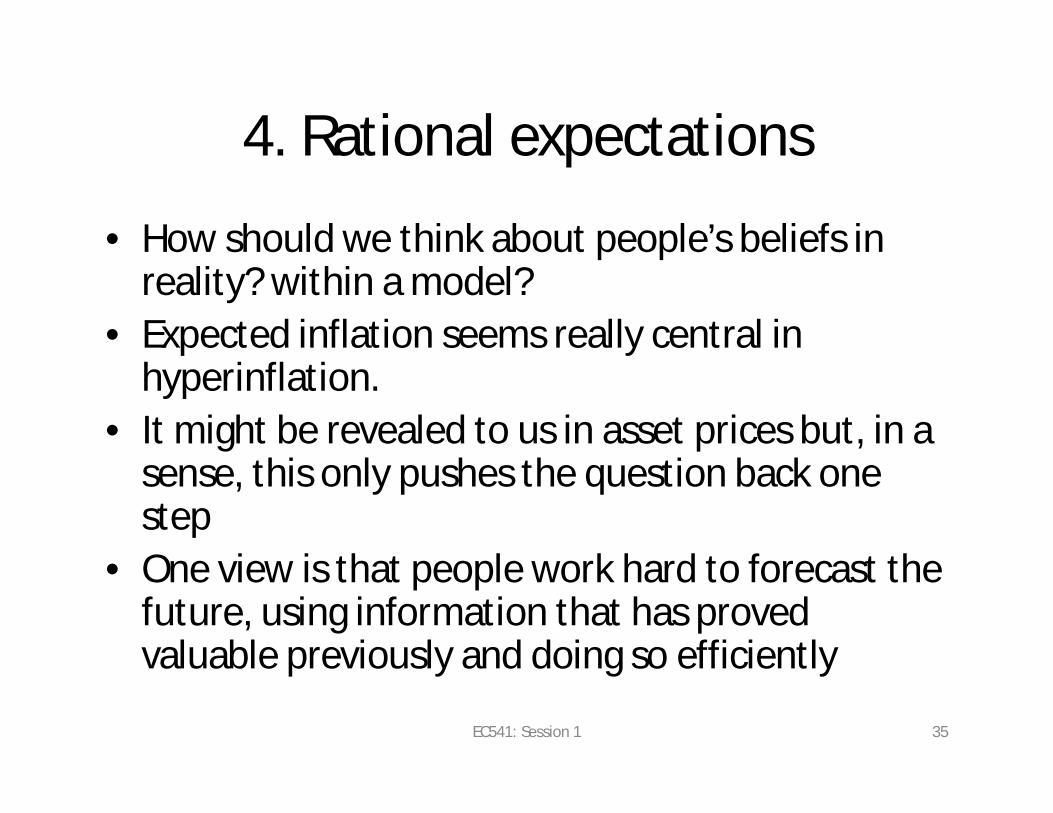
4. Rational expectations

• How should we think about people’s beliefs in reality? within a model?

• Expected inflation seems really central in hyperinflation.

• It might be revealed to us in asset prices but, in a sense, this only pushes the question back one step

• One view is that people work hard to forecast the future, using information that has proved valuable previously and doing so efficiently

EC541: Session 1 35

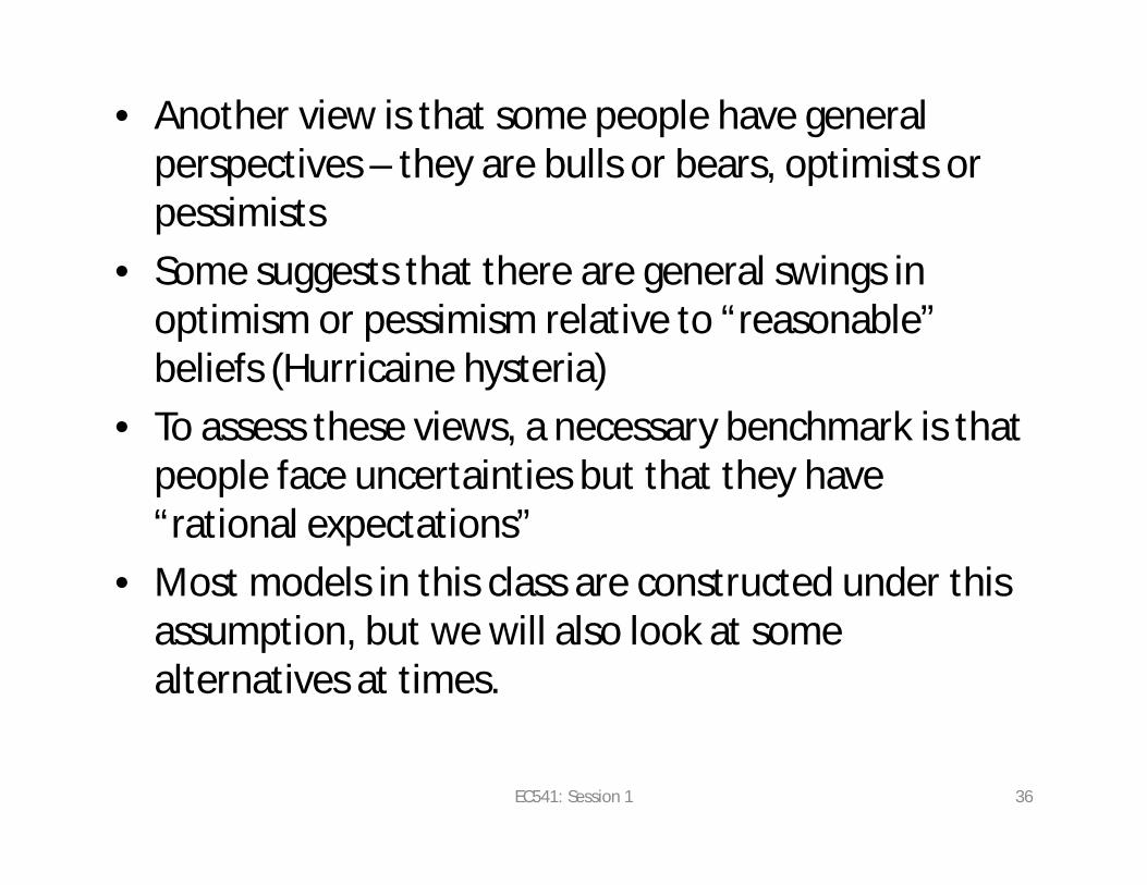
• Another view is that some people have general perspectives – they are bulls or bears, optimists or pessimists

• Some suggests that there are general swings in optimism or pessimism relative to “reasonable” beliefs (Hurricaine hysteria)

• To assess these views, a necessary benchmark is that people face uncertainties but that they have “rational expectations”

• Most models in this class are constructed under this assumption, but we will also look at some alternatives at times.

EC541: Session 1 36

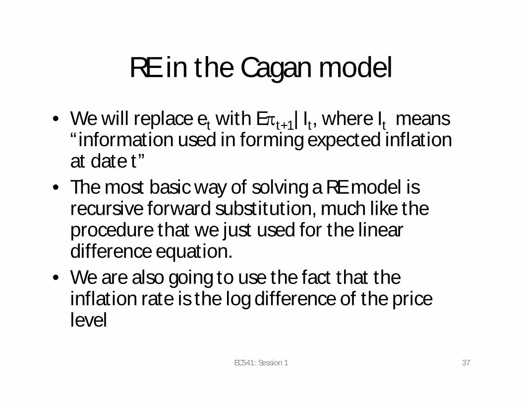
RE in the Cagan model

• We will replace et with Ept+1|It, where It means “information used in forming expected inflation at date t”

• The most basic way of solving a RE model is recursive forward substitution, much like the procedure that we just used for the linear difference equation.

• We are also going to use the fact that the inflation rate is the log difference of the price level

EC541: Session 1 37

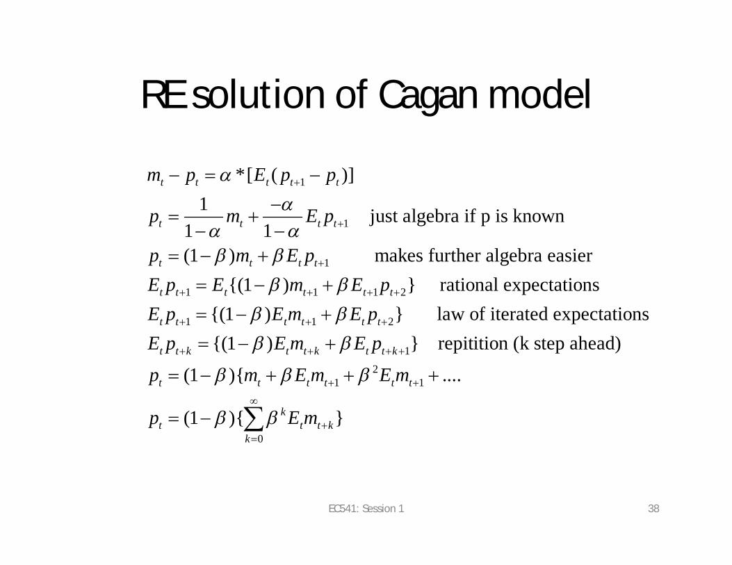
RE solution of Cagan model

EC541: Session 1 38

1

1

1

1 1 1 2

1

*[ ( )]1 just algebra if p is known

1 1(1 ) makes further algebra easier

{(1 ) } rational expectations{(1 )

t t t t t

t t t t

t t t t

t t t t t t

t t t t

m p E p p

p m E p

p m E pE p E m E pE p E m

1 2

12

1 1

0

} law of iterated expectations{(1 ) } repitition (k step ahead)

(1 ){ ....

(1 ){ }

t t

t t k t t k t t k

t t t t t t

kt t t k

k

E pE p E m E pp m E m E m

p E m

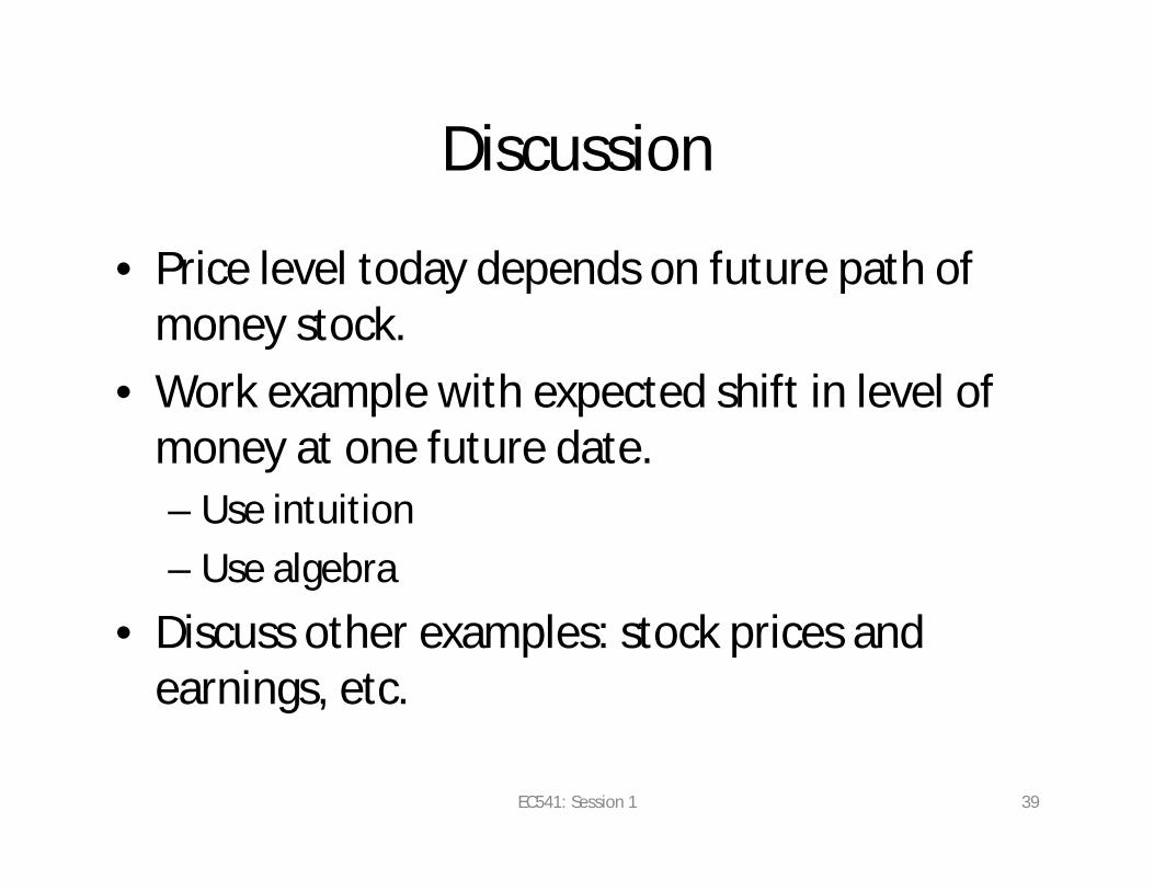
Discussion

• Price level today depends on future path of money stock.

• Work example with expected shift in level of money at one future date. – Use intuition– Use algebra

• Discuss other examples: stock prices and earnings, etc.

EC541: Session 1 39

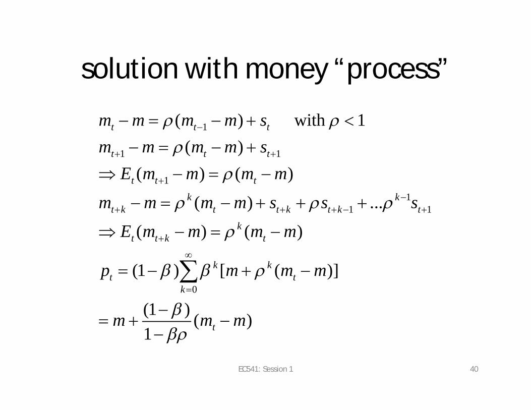
solution with money “process”

EC541: Session 1 40

1

1 1

11

1 1

0

( ) with 1( )

( ) ( )

( ) ...

( ) ( )

(1 ) [ ( )]

(1 ) ( )1

t t t

t t t

t t tk k

t k t t k t k tk

t t k t

k kt t

k

t

m m m m sm m m m s

E m m m mm m m m s s s

E m m m m

p m m m

m m m

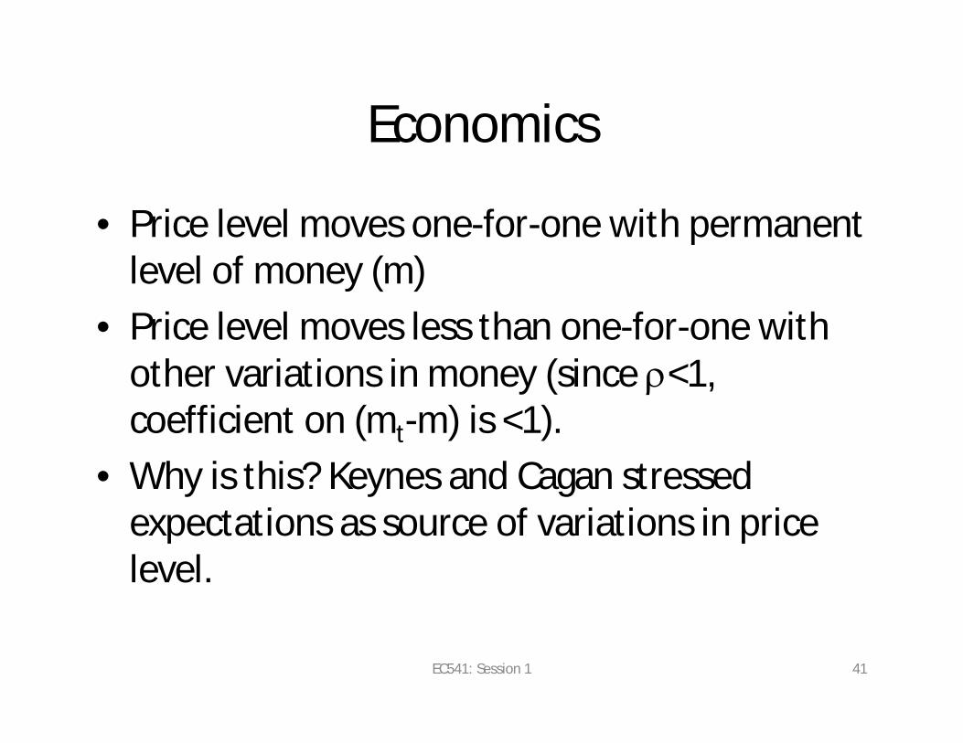
Economics

• Price level moves one-for-one with permanent level of money (m)

• Price level moves less than one-for-one with other variations in money (since r<1, coefficient on (mt-m) is <1).

• Why is this? Keynes and Cagan stressed expectations as source of variations in price level.

EC541: Session 1 41

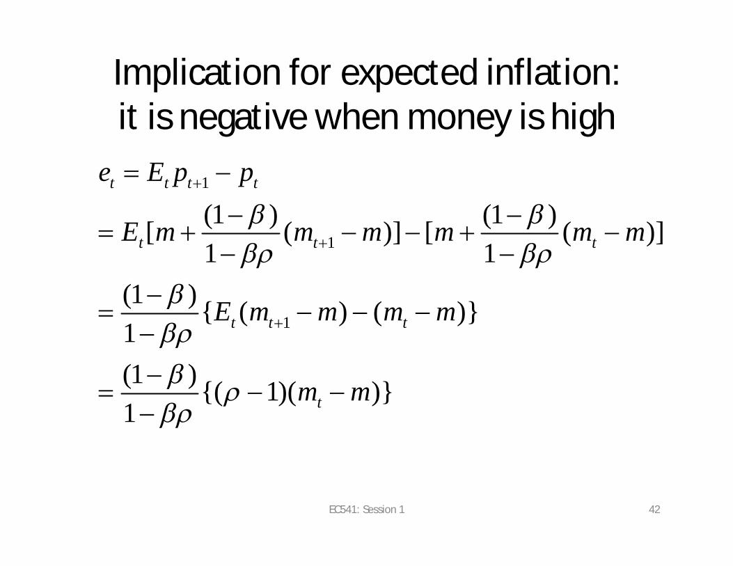
Implication for expected inflation: it is negative when money is high

EC541: Session 1 42

1

1

1

(1 ) (1 )[ ( )] [ ( )]1 1

(1 ) { ( ) ( )}1(1 ) {( 1)( )}1

t t t t

t t t

t t t

t

e E p p

E m m m m m m

E m m m m

m m

EC541: Session 1 43

Link to Lucas• Suppose that money has two parts: permanent and

transitory variations

• Then, must smooth out transitory parts to find classical link between money and price level (Lucas does for money growth and inflation, but idea is same) or hold expected inflation fixed

EC541: Session 1 44

1

1

[ trend or permanent component]

[serially correlated but transitory]

t t t

t t t

t t xt

m xs

x x s