class: catchment scale multiple-landuse...

C O O P E R A T I V E R E S E A R C H C E N T R E F O R C A T C H M E N T H Y D R O L O G YC O O P E R A T I V E R E S E A R C H C E N T R E F O R C A T C H M E N T H Y D R O L O G Y

Established and supportedunder the Australian

Government’s CooperativeResearch Centre Program

The Cooperative Research Centre forCatchment Hydrology is a cooperativeventure formed under the AustralianGovernment’s CRC Programmebetween:

• Brisbane City Council

• Bureau of Meteorology

• CSIRO Land and Water

• Department of Infrastructure,Planning and Natural Resources,NSW

• Department of Sustainability andEnvironment, Vic

• Goulburn-Murray Water

• Grampians Wimmera Mallee Water

• Griffith University

• Melbourne Water

• Monash University

• Murray-Darling Basin Commission

• Natural Resources, Mines andEnergy, Qld

• Southern Rural Water

• The University of Melbourne

ASSOCIATE:

• Water Corporation of WesternAustralia

RESEARCH AFFILIATES:

• Australian National University

• National Institute of Water andAtmospheric Research, New Zealand

• Sustainable Water ResourcesResearch Center, Republic of Korea

• University of New South Wales

INDUSTRY AFFILIATES:

• Earth Tech

• Ecological Engineering

• Sinclair Knight Merz

• WBM

CENTRE OFFICECRC for Catchment HydrologyDepartment of Civil EngineeringBuilding 60 Monash University Victoria 3800 Australia

Tel +61 3 9905 2704Fax +61 3 9905 5033email [email protected]

CLASS: CATCHMENT SCALE MULTIPLE-LANDUSEATMOSPHERE SOIL WATER AND SOLUTE TRANSPORTMODEL

TECHNICAL REPORTReport 04/12

December 2004

Narendra Kumar Tuteja / Jai Vaze / Brian Murphy / Geoffrey Beale

Tuteja, Narendra Kumar.

CLASS: Catchment Scale Multiple-LanduseAtmosphere Soil Water and Solute TransportModel.

Bibliography

ISBN 1 920813 17 9

1. Hydrologic models. 2. Runoff - Mathematical models. I. Tuteja,Narendra Kumar. II. Cooperative Research Centre for CatchmentHydrology. III. Title. (Series : Report (Cooperative Research Centre forCatchment Hydrology); 04/12)

551.48011

Keywords

Land useCatchment areasModelsSoil waterSolutesTransportWater yieldSalinitySaltingGeographic information systemsWater balanceSpatial distributionVegetationPasturesHydrologyRechargePlant water relations

© Cooperative Research Centre for Catchment Hydrology, 2004

COOPERAT IVE RESEARCH CENTRE FOR CATCHMENT HYDROLOGY

i

CLASS: CatchmentScale Multiple-Landuse AtmosphereSoil Water andSolute TransportModel

Narendra Kumar Tuteja / Jai Vaze / BrianMurphy / Geoffrey Beale

Department of Infrastructure, Planning andNatural Resources, New South Wales, Australia

Technical Report 04/12December 2004

Preface

Since the beginning of computer based hydrologicalmodels in the 1960s and 1970s, there has been muchdebate regarding the appropriate structure and levelof complexity of models. This reached fever pitch inthe late 1980s and early 1990s as the cost ofcomputing power reduced dramatically and a newgeneration of models provided information not onlyat catchment outlets, but also simulation of thespatial responses within the catchment. These are socalled “process-based, distributed models” and themost complex of them are based on fundamentalequations for the movement of water and solutesthrough porous media, hydraulic and hydrodynamicbehaviour. They are characterised as “bottom-up”models where algorithms related to the myriad ofprocesses that make up hydrological response arelinked together, resulting in models with a very largenumber of parameters, many of which are “inprinciple” measurable but in practice can be difficultto define.

These models contrast with the “top-down” style ofmodels that are conceptually simpler with fewerempirical parameters that are generally calibratedagainst observations, but are more limited in spatialdetail and process representation. The modellingliterature, particularly from the 1990s, includes manydiscussions on the philosophical, theoretical andpractical advantages and disadvantages of the variousapproaches to modelling, with often quite polarisedviews.

In more recent times, there has been a wideracceptance of “horses for courses” – the need for arange of models of different complexity to meet thewide range of modelling applications and dataavailability. This technical report describes themodelling framework, CLASS, which is at the morecomplex end of the modelling spectrum, but wherethere has been a major effort made to exploit theever-increasing range of available data for setting upand running the model. CLASS was developed bythe New South Wales Department of Infrastructure,Planning and Natural Resources as an AssociateProject of the Cooperative Research Centre (CRC)for Catchment Hydrology.


i i

CLASS is a distributed, eco-hydrological modellingframework that deals with water and solutemovement from hillslope to catchment scale.Considerable effort has been made in representingvegetation growth, as well as in the pathways thatwater takes from hillslope to stream. This capabilityenables detailed simulation of the effects of differentmanagement scenarios. CLASS includes user-friendly interfaces to assist the user in preparing thedata needed for execution and testing. The sciencethat underpins CLASS has been externally reviewedand is clearly described in this report.

Ultimately, CLASS will be incorporated into theCatchment Modelling Toolkit (www.toolkit.net.au)and will be one of a number of models of differentcomplexity that represent water and solutemovement. The CLASS modelling frameworkincludes seven products that can be implemented atthe hillslope scale. However, at the catchment scaleCLASS is a computationally demanding modellingapproach, and requires considerable skill to applyand interpret the model results, but is a powerfulplatform for detailed analysis and makes excellentuse of the available data.

Rodger Grayson, DirectorCRC for Catchment Hydrology


ii i

Acknowledgments

We wish to acknowledge the following for theircontributions: John Gallant, Ian Johnson, Jim Morris,Jin Teng, Bill Johnston, David Tarboton, YuriIvailovski, Guy Geeves, Greg Summerell, MichelleMiller, Michael Williams and Sanmugan Prathapar.We thank Ross Williams, Dugald Black, Peter Barkerand Charmaine Beckett for their support. New SouthWales Government funded the work under the NSWSalinity Strategy. We thank Mark Wigmosta (PacificNorthwest National Lab., Richland, USA), TomasVogel (Czech Technical University, Prague, CzechRepublic) and Rodger Grayson (CRC for CatchmentHydrology, Australia) for reviewing this work. Thisreport has improved substantially from their review.


i v


v

Preface i

Ackowlegements iii

List of Figures vii

1. Introduction 1

2. Overview of the CLASS Modelling Framework 3

3. CLASS Water Balance and Plant Growth Components 7

3.1 Climate Data and Disaggregation of Daily ClimateData to Sub-daily Climate Data 7

3.2 Topographic Modelling 7

3.2.1 Topographic Modelling for Estimation of the Spatial Distribution of Soils 7

3.2.2 Topographic Modelling for Estimation of the Soil Depth and Soil Moisture Storage 8

3.2.3 Topographic Modelling for Determining Hydrological Flow Paths and the Upstream Contributing Areas 8

3.3 Soil Pedotransfer Function (PTF) ModelsFor Parameterisation of the Soil Hydraulic Properties 8

3.4 Multiple Landuse and Radiation Balance Model 9

3.5 Interception Model 10

3.6 Infiltration Model 12

3.7 Evapotranspiration Sub-model 12

3.7.1 Aerodynamic and Canopy Resistance 13

3.7.2 Comparison with Pan Evaporation Data 17

3.8 Pasture Growth Model (Class PGM) 18

3.9 Crop Growth Model (Class CGM) 18

3.10 Tree Growth Model (Class 3PG+) 19

3.11 Unsaturated Moisture Movement Model (Class U3M) 19

3.11.1 Mass Balance 19

3.11.2 Boundary Conditions 22

3.11.3 Numerical Solution 23

3.12 Horizontal Redistribution and Sub-surface Flow from Each Soil Material 26

3.13 Soil Material Water Balance 29

3.14 Generated Surface Runoff, Groundwater Runoff and Runoff Routing 30

3.14.1 Generated Surface Runoff 30

3.14.2 Generated Groundwater Runoff and Lateral Throughflow 31

3.14.3 Surface Runoff Routing 34

3.14.4 Groundwater Routing 34

4. CLASS Solute Balance Components 35

4.1 Determining Discharge Areas in a Catchment 35

4.2 Current In-stream Solute Export Model 35

4.3 Solute Mass Balance Over the Soil Material 35

4.4 Solute Transport in the Stream 37


v i

5. Time Stepping 39

6. Data Requirements and Model Parameters 41

6.1 Spatial Data Requirements 41

6.2 Temporal Data Requirements 41

7. Summary 43

8. Software Platform Related Issues 45

9. References 47


vi i

List of Figures

Figure 1. The CLASS Modelling Framework 4

Figure 2. Schematic Diagram of Partitioning of the WaterBalance Components and Simulated Landuse 5

Figure 3. Schematic Diagram of the Energy Distribution forPartial Canopy 15

Figure 4. Three Layered Distribution for Estimation of theAerodynamic Resistance 16

Figure 5. Schematic Showing Estimation Procedure of theAerodynamic Resistance for Partial Canopy 17

Figure 6. Schematic Diagram of the Soil Layer System with L Discrete Soil Layers and M Soil Materials 19

Figure 7. Schematic Diagram for Apportioning of the Flow �pk from Pixel p to Pixels 4 and 5 21

Figure 8. Schematic Diagram Showing Accumulation of the Flow from Upslope Pixels 0, 1, 2, 3, 6 and 7 to Pixel p 21

Figure 9. Schematic Diagram of Partitioning of the WaterBalance Components and Simulated Landuse 30


vii i


1

1. Introduction

Investigation of the vegetation effects in theatmosphere-soil-vegetation continuum on thecatchment scale water balance has been a subject ofextensive observation and modelling across the worldfor many years (Vertessy et al., 1996). Complexdistributed parameter process models such as SHE(Abbott et al., 1986), TOPOG_IRM (Dawes andHatton, 1993) and CATPRO (Ruprecht and Sivapalan,1991) have been used to address these issues. Whilevery useful, they require comprehensive calibrationdata sets to parameterise the many micro-scaleprocesses incorporated in their procedures. As suchthey are used primarily as research tools rather thanmanagement tools. Process based one dimensionalwater balance models such as PERFECT (Littleboy etal., 1992) and APSIM (McCown et al., 1996), havebeen used in a GIS framework to investigate theeffects of soils, landuse and land managementpractices on the near surface soil moisture dynamicsand water balance components (eg. Ringrose-Voaseand Cresswell, 2000). However, there is often amismatch between the catchment scale fluxes andthose obtained in a purely vertical analysis due to scaleeffects and no accounting of the lateral fluxes.

In recent times complex process modelling approacheshave given way to more simplistic approaches due toissues of scale and data availability (Grayson andBlöschl, 2000). Many authors (eg. Holmes andSinclair, 1986; Turner, 1991; Zhang et al., 2001) havedeveloped relationships between vegetation type andaverage annual evapotranspiration from a smallnumber of readily available parameters. Althoughuseful, these coarse average annual relationshipsprovide insufficient information on the temporaleffects of tributary flow required for watermanagement purposes.

In upland areas with moderate to steep slopes,topography is an important variable that affects waterbalance and the magnitude of lateral fluxes inconjunction with the spatial distribution of soil typesand landuse. Several topographic indices relatinglandscape position to surface and sub-surface runoffare commonly used (eg. Roberts et al., 1997). Themost commonly used index is called the wetness index

(Beven and Kirkby, 1979) that under somecircumstances (Grayson and Western, 2001) can beused to quantify runoff potential of different landscapeelements. This index can be used to relate depth of the(perched) water table at any location in the catchmentto mean depth of the (perched) water table over thecatchment as in the TOPMODEL (Beven and Kirkby,1979). The wetness index incorporates the effect oftopography but does not account for the effects of soilsand landuse. Therefore, a common situationencountered in catchment scale modelling is eitherinadequate accounting of the scale effects and lateralfluxes or inadequate accounting of the soil andvegetation effects.

A new generation of the distributed hydro-ecologicalmodels has been developed or is under developmentthat attempt to simplify the complexity of applying atightly bound theory and iterative numericalcomputations as in SHE and TOPOG. These modelsattempt to simplify excessive parameterisation and thenumerical complexity associated with the distributedmodels. The structure of these models still retains therelevant internal processes of the climate-vegetation-soil-topography continuum and the relevant boundaryconditions within the modelling paradigm. Examplesof these models include various implementations ofthe TOPMODEL (Beven and Kirkby, 1979;Famiglietti et al., 1992; Band et al., 1993; Sivapalan etal., 1997; Beven and Freer; 2001), HILLFLOW-3D(Bronstert, 1995), DHSVM (Wigmosta et al., 1994),MACAQUE (Watson et al., 1999; Watson et al., 2001)and CATSALT (Tuteja et al., 2003; Vaze et al., 2004).

It is generally accepted that the spread of drylandsalinity in the upper parts of the Murray-Darling Basinhas resulted from the clearing of native vegetation forEuropean-style agriculture (Walker et al., 1992;Williamson et al., 1997). A system of water qualitytargets, benchmarked at major basin outlets andstrategic locations within each river basin network hasbeen adopted (DLWC, 2000; MDBMC, 2001). Thesetargets are intended to also facilitate the developmentof markets in salinity, carbon and biodiversity credits.A prerequisite for salinity management is modelling ofthe impacts of landuse change on water yields, saltexport, and aquifer response times, to assess thebiophysical capacity to change. CATSALT version 1.5was developed to support assessment of the catchment


2

scale impacts of realistic and plausible landusechanges on stream flow and salinity (Vaze et al., 2004;Tuteja et al., 2003). It uses semi-distributed water andsalt balance and a comprehensive framework fordescribing soil hydraulic properties and soil salinities.

CATSALT version 1.5 was developed as anintermediate product to support policy initiatives withregards to salinity. While the product has served itsintended purpose and is better than most salinitymodelling tools available in Australia, there are manylimitations of version 1.5 that must be overcome, suchas:

• CATSALT version 1.5 uses topographic wetnessindex as the basis for all computations. Manydifferent landscape elements in the catchment canhave the same wetness index. This producesdifficulties in implementing landuse changescenarios.

• Averaging of salt concentration over the wetnessindex categories in the soil is unavoidable and thishas implications for salt modelling.

• CATSALT version 1.5 apportions flow at thecatchment outlet based on landuse and the wetnessindex or topography without explicit routingthrough the landscape. Effects of landuse changescenarios in a property can be seen at the catchmentoutlet and not at the properties at downstreamlandscape locations.

• CATSALT version 1.5 does not include vegetationgrowth and depends on other models (eg.PERFECT; Littleboy et al., 1992).

A quantitative analysis of the impacts of climate andlanduse change on water and salt yield from acatchment can be undertaken using a distributedhydrological model that can adequately representsystem dynamics of the complex hydrologicalprocesses and operates on a pixel level. To overcomethe above limitations, we have created a newdistributed model, called the Catchment scalemultiple-landuse atmosphere soil water and solutetransport model (CLASS). The model is adapted toAustralian conditions and is designed for accurateassessment of the paddock scale effects of landusechanges and climate variability on water and salt yieldfrom the catchment. Our approach differs from earlierapproaches in that the model is being designed to

operate in data poor environments with the appropriatelevel of complexity. The distributed model DHSVM(Wigmosta et al., 1994) is somewhat similar to ourobjectives and approach. Therefore where appropriate,parts of the water balance component of CLASS areadapted from DHSVM. This technical report describeskey components of the CLASS model in detailincluding all the principal algorithms and theassociated equations.


3

2. Overview of the CLASS Modelling Framework

The CLASS modelling framework consists of a suiteof tools that can be used for physically baseddistributed eco-hydrological modelling (Figure 1).The framework is designed for investigation of theeffects of landuse and climate variability on bothpaddock scale as well as the catchment scale. Theframework includes the following tools that are usedas building blocks in the catchment model.

CLASS Spatial Analyst - a fully automated GISbased tool required for spatial modelling (Teng et al.,2004; released May 2004). It prepares all spatialinformation required by the catchment model. Thisincludes: preparation of the climate surfaces anddelineation of the climate zones, determination of thesoil depth, water balance computational sequenceusing multiple flowpaths from terrain analysis andflow accumulation areas, wetness index, landdischarge areas, soil salinity distribution and mappingof pixels to landuse and groundwater flow systems. Adynamic but constant user specified pixel size can beused depending on DEM resolution and size of theproblem.

CLASS U3M-1D - a variable sub-daily time stepmodel used for partitioning water balance in theunsaturated zone using the Richard’s equation on asingle pixel (Vaze et al., 2004; released June 2004).Solutes are transferred between the soil materialsusing advection.

CLASS U3M-2D - a variable sub-daily time stepmodel used for partitioning water balance in theunsaturated zone using the Richard’s equation on ahillslope (Tuteja et al., in prep. a). Solutes aretransferred between the soil materials using advection.

CLASS PGM - a daily time step growth model basedon Johnson (2003) that simulates up to five multiplepasture species that may be summer or winter activeperennial/annual pasture and a legume (Vaze et al.,2004a). Environmental conditions as well as soilwater, nutrient and salinity status influences pasturegrowth and tissue dynamics.

CLASS CGM - a daily time step growth model basedon Johnson (2003) that simulates a generic crop and its

physiological structure and allows for complexinteractions between light, temperature, availablewater and nutrients (Vaze et al., 2004b).

CLASS 3PG+ - a monthly time step growth modelthat simulates tree growth using the 3-PG+ model(Morris, 2003), an adaptation of the 3PG model byLandsberg and Waring (1997) (Tuteja et al., in prep.b).

CLASS Catchment Model - a distributed catchmentscale model described in this report that operates on apixel level and makes use of the above tools (Figure2.2). Climate data and landuse information is used ateach pixel for plant growth using CLASS PGM, CGMand 3PG+. Unsaturated zone water and solute balanceis then performed using U3M-1D along the verticalaxis. Excess moisture and the associated solutes arethen estimated over each soil material. Water andsolutes are transferred from up-slope properties to thedown-slope properties and eventually to the catchmentoutlet using multiple flow paths and Darcian concepts.Additionally, spatial distribution of the soils, landuse,climate and groundwater flow system (GFS) linkspixel scale dynamics to the catchment scale effects.Recharge and lateral throughflow each are pooled overthe GFS. A proportion of each of these components ispassed to the land as surface discharge and theremaining component is passed to the stream.Discharge to the land and stream is laggedappropriately and is based on the assumption that thebulk of the travel time results where the flow occursunder phreatic conditions, and that a fast pressuretransmission signal applies under the confinedconditions. Routing in the stream is based on theresponse function approach (Nash, 1960; Kachroo,1992).

The model design accounts for data constraints oftenimposed in catchment scale investigations. Datarequirements vary depending on the type ofimplementation ie. property scale or the catchmentscale. The following primary data are required forimplementation of the CLASS framework: climatedata, DEM, Landuse, FLAG upness index, MRVBFindex, GFS spatial distribution, hydraulic propertiesand solute concentration, soils spatial distribution, soilhydraulic properties, growth parameters, observedflow and solute concentration. Most of these data are


4

available on a wide spread basis. Sufficient tools anddatabases exist in the CLASS framework that allowsfor generating the information generally not availablefor catchment scale implementations (eg. soils, growthparameters and terrain analysis). All parametersrequired for the CLASS Catchment Model aredescribed in the User’s Manual (Tuteja et al., inprep.c)

The CLASS modelling framework is supported by auser friendly graphical user interface. In 2004-05, theCLASS modelling framework will be incorporatedinto Toolkit Modelling Environment developed by theCooperative Research Centre for CatchmentHydrology (Rahman et al., 2003).

Figure 1. The CLASS Modelling Framework.


5

Figure 2. Schematic Diagram of Partitioning of the Water Balance Components and Simulated Landuse:- (a) solarradiation and climate data, (b) rainfall, (c) evapotranspiration, (d) overland flow, (e) flow through the soil, (f)shallow sub-surface flow, (g) drainage from the soil profile and recharge to the Groundwater Flow System(GFS), (h) water balance computational sequence (1-9), (i) discharge from groundwater to land and stream.


6


7

3. CLASS Water Balance and Plant Growth Components

3.1 Climate Data and Disaggregation ofDaily Climate Data to Sub-daily ClimateData

Daily climate surfaces are available in Australia fromthe Silo database archived at Queensland Departmentof Natural Resources (Jeffrey et al., 2001). Availableclimate data includes maximum and minimum airtemperature, rainfall, pan evaporation, incomingshort-wave radiation, vapour pressure, maximum andminimum humidity. Climate surfaces are available at 5 km grid for the whole of NSW and are used todescribe climate forcing on the soil surface. In generalfour to six climate zones are formed and each pixel inthe catchment is linked to a given climate zone todescribe the atmospheric boundary condition.

Rainfall intensity relevant to the runoff generationmust be reflected in the temporal resolution of themeteorological data and the modelling time step.Average rates over a time interval are invariablytreated as constant rates within the time step in mostmodels. If the time intervals are long (eg. 24 hours),the replacement of actual, highly variableinstantaneous precipitation rates with daily averagesmay lead to an intolerably high underestimation of theoverland flow and overestimation of the infiltration(Kandel et al., 2002). Similar arguments pertain, to alesser extent, to the soil evaporation rate, where theuse of daily averages can lead to an unrealisticoverdrying of the uppermost soil layer (Dolezal,2002). It may be argued that the overall long-termhydrological behaviour of a soil profile can besatisfactorily modelled even if the fine diurnaldynamics is neglected.

In order to define the atmospheric boundary conditionat the soil surface, an accurate estimate of the climatefluxes at a sub-daily time step is required.Disaggregation of the daily climate data into sub-dailyclimate data is adapted from Dolezal (2002). Forrainfall disaggregation, an exponential distributionform is used and is adapted from the EPIC model(Sharpley et al., 1990). Disaggregation of the potentialevapotranspiration uses clear sky irradiance and is

adapted from the work of a number of authors (eg.Beer, 1990; Burman and Pochop, 1994; Burman et al.,1983; Monteith and Unsworth, 1990; Smith, 1991)

3.2 Topographic Modelling

3.2.1 Topographic Modelling for Estimation ofthe Spatial Distribution of Soils

Estimates of soil hydraulic properties across thelandscape are a requirement for implementation of adistributed hydrologic model. Unfortunately there arefew direct data on soil hydraulic properties at acatchment scale. Estimates of these properties have tobe made using relationships based upon moreroutinely and more frequently collected soil propertymeasurements. While a considerable amount has beenwritten about the development of parametricPedotransfer Functions (PTFs) to relate various soilphysical, chemical and morphological properties tosoil hydraulic properties, less has been written abouthow they can be applied to catchments. Spatialdistribution of the individual soil types withinindividual soil landscapes is predicted using a DEMand terrain analysis and the framework of Murphy etal., (2003).

Soil landscape units are frequently mapped and theseare commonly topographic sequences of soils, withdifferent soil types occupying different landformelements. The usual sequence consists of shallower,well-drained soils on crests and upper slopes, gradingto deeper, poorly drained soils on lower slopes anddepressions. Alluvial soils are associated withdefinable floodplains and terraces. The FLAG model(Roberts et al., 1997) is used for terrain analysis tosub-divide the catchment into four slope classes (low,low to mid, mid to upper and upper slopes) to separateareas of individual soil types within soil landscapes(McDonald et al., 1990; Summerell et al., 2003a-b).The four slope classes are also referred to as the FLAGlandforms. This enables prediction of the spatialdistribution of individual soil types. The methodologymakes the best possible use of the available soilinformation from soil maps, data bases, and secondarysources of information such as geology maps,geomorphology maps, and climate data. It is clear thatthis particular methodology assumes that thedistribution of soil types within a soil landscape isdefined by a toposequence. Where some other factors


8

control the distribution of soil types in a landscape,such as microclimate or short-range variation in parentmaterials, the methodology needs to be modified. Afurther complication occurs in using soil maps wherea single toposequence is divided into two soillandscapes, as can occur with some more intensivemapping.

The identification of soils down to the soil type levelenables the texture, structure and bulk density of theindividual soil horizons to be predicted. Theassumption is made that each Great Soil Group (Staceet al., 1968) within a soil landscape is equivalent to asoil family or soil series. Relationships betweentexture and structure and soil hydraulic properties thathave been developed in the literature and from otherdata sets are then used to predict the soil hydraulicproperties of the individual soil types (see Section3.3).

3.2.2 Topographic Modelling for Estimation ofthe Soil Depth and Soil Moisture Storage

Soils on the hillslopes are generally shallow and thelandscape processes are characterised by erosion whiledeeper soils in deposition environment occur on thevalley bottoms. Distinguishing valley bottoms fromhillslopes is important to determine soil depths andsoil moisture holding capacities across the landscape.Gallant and Dowling (2003) have presented a newindex, called the Multi-Resolution Valley BottomFlatness index (MRVBF) for delineating depositionalareas from the erosion areas high in the landscape.Their methodology operates at a range of scales andcombines the results at different scales into a singleindex that can be related to predict soil depth and soilmoisture storage capacity.

McKenzie et al., (2003) presented a methodology topredict soil depth and soil moisture storage capacityfor medium sized catchments. They predicted soildepth based on the wetness index and MRVBF in theerosional and depositional landscapes respectively. Asmooth weighting function was introduced that gavemore weightage to wetness index at locations high inlandscape. The weighting for wetness index decreasesgradually while MRVBF weighting increases atlocations low in the landscape. This framework is usedin CLASS along with spatial distribution of the soils topredict soil depth and soil moisture storage capacity.

3.2.3 Topographic Modelling for Determining Hydrological Flow Paths and the UpstreamContributing Areas

Many schemes are available for calculatinghydrological flowpaths and the upstream contributingarea at any given location in the catchment (eg.O’Callaghan and Mark, 1984; Quinn et al., 1991; Lea,1992; Costa-Cabral and Burges, 1994; Tarboton,1997). Tarboton (1997) proposed a new multiple flowpath algorithm, called the D∞ method, that performedbetter than most other methods.

This method is used in CLASS for estimatinghydrological flowpaths and is used for horizontaldistribution of the saturated sub-surface flow byadvection. The method is based on representingresultant flow direction as a single angle taken as thesteepest downward slope on the eight triangular facetscentred at each grid point. Flow is then apportioned tothe two-downslope pixels on the basis of anglebetween the resultant flow direction and the angles ofthe downslope pixels.

3.3 Soil Pedotransfer Function (PTF) Modelsfor Parameterisation of the SoilHydraulic Properties

Spatial distribution of soils in the catchment and theirphysical properties (eg. texture, structure, soilhorizons and bulk density etc.) are determined usingthe methodology of Murphy et al., (2003) (Section3.2.1). Parametric PTFs can then be used to estimatesoil hydraulic parameters describing variation ofpressure head with soil moisture and unsaturatedhydraulic conductivity (eg. Wösten et al., 1995;Schaap et al., 1998; Minasny and McBratney, 2002).Minasny and McBratney (2002) proposed a newmethod called the neuro-m method, whereinparameter estimation by the artificial neural network ismatched against the measured data. Using Australiandata as a training set these authors demonstratedsubstantial improvement in accuracy of the PTFsobtained from neuro-m method compared to thoseobtained from published neural network based PTFs.This method is used for estimating soil hydraulicparameters of the van Genuchten’s soil hydraulicmodel (van Genuchten, 1980). Two additional soilhydraulic models by Vogel and Cislerova (1988) andBrooks and Corey (1966) are also available in CLASS


9

U3M. Preset soil parameters based on the soil type arealso built into the model from published databases(Carsel and Parrish, 1988; van Genuchten et al.,1991).

3.4 Multiple Landuse and Radiation BalanceModel

The overstory shortwave radiation balance accountsfor canopy reflectance, ground cover, radiationattenuation and is given by Equation 3.4.1.

(3.4.1)

where:

= shortwave radiation absorbed by theoverstory (Wm-2),

= incident shortwave radiation (Wm-2),

= overstory albedo (-),

= canopy attenuation coefficient (-),

= overstory LAI,

= overstory groundcover fraction (-).

The understory receives attenuated shortwaveradiation from the overstory and direct shortwaveradiation where there is no overstory (see Equation3.4.2).

where:

= shortwave radiation absorbed by theunderstory (Wm-2),

= understory albedo (-),

= understory LAI.

Shortwave radiation absorbed by the soil surfaceincludes attenuated radiation from the understory andis given by Equation 3.4.3.

where:

= shortwave radiation absorbed by the soil surface (Wm-2),

= ground surface albedo (-).

The overstory longwave radiation balance is given byEquation 3.4.4.

where:

= absorbed overstory longwave radiation (Wm-2),

== downward longwave radiation (Wm-2),

= air temperature above the canopy (ºC),

=

= clear sky atmospheric emissivity (-)(Idso, 1981),

= overstory temperature (assumed same as the air temperature ºC),

= vapour pressure (mb),

= understory temperature (assumed same asthe air temperature ºC),

= Stefan-Boltzmann constant (Wm-2K-4).

(3.4.2)

(3.4.3)

(3.4.4)

(3.4.5)

sgR

g

loR

dL

aT

a

oT

ae

uT

++ ))273/(1500exp(1095.57.0 5aa Te

+ 4)273( aa T


1 0

The understory longwave radiation balance with theoverstory and ground is given by Equation 3.4.5.

where:

= absorbed understory longwave radiation (Wm-2),

= soil surface temperature (assumed sameas the air temperature ºC).

Longwave radiation balance of the ground surface isgiven by Equation 3.4.6.

where:

Rlu = absorbed understory longwaveradiation (Wm-2 ).

The climate variables Rs,Rsj,Tj,Tg and Ld vary in time(d) and are averaged over the climate zone (j refers toeither the overstory or the understory). The landusevariables LAIj and Fj vary in time (d) and space (pixel)and are obtained from the growth models (Sections3.8, 3.9 and 3.10).

3.5 Interception Model

The interception storage capacity for a canopy j for agiven time step (t��t) is estimated from LAI at theend of previous time step (t) (Dickinson, 1991;Wigmosta et al., 1994).

(3.5.1)

where:

Icj = Interception storage capacity of thecanopy with j representing either theoverstory Ico or the understory Icu (m),

Fj = ground cover fraction of the canopy j.

Under growth limiting conditions imposed mainly by

vapour pressure deficits, LAI for the overstorygenerally reaches a maximum of 4 (Landsberg andWaring, 1997). Assuming ground cover fraction to beone, maximum interception storage capacity of 0.4 mmis obtained for the overstory. This is similar to theinterception storage capacity of 0.35 mm for theevergreen forest canopy obtained from experimentalobservations by Dunin et al.,(1988). For pasture andcropping, interception storage capacity would varybetween 0 and 0.4 mm.

Denoting interception storage as Sij(m), potentialevaporation (Epjm.s -1) from the wet canopy (Sij>0) isobtained as in Equation 3.5.2.

where:

Rnj = net absorbed radiation ie. sum of canopy shortwave and longwave radiation (W.m-2),

� = density of the moist air (kg.m-3),

Cp = specific heat of the air (J.kg -1.K -1),

ea,es = vapour pressure and saturated vapourpressure respectively at a given airtemperature (mb) (Equation 3.5.10),

raj = aerodynamic resistance of the canopyj(s.m -1),

� = psychrometric constant (mb.K-1),

� = slope of the saturated vapour pressure-temperature curve (mb.K-1) (Equation3.5.11),

λ = latent heat of vaporisation (J.kg -1),

�w = density of water (kg.m-3).

(3.4.6)

(3.5.2)

luR

gT

(3.5.3)


1 1

Computation procedure for the aerodynamicresistance is described in Section 3.7.1. Actualevaporation from the canopy interception storage (Eij m.s-1) is constrained as minimum of moistureavailable in interception storage and the potentialevaporation (see Equation 3.5.3).

Actual interception storage of the overstory iscalculated as in Equation 3.5.4.

where:

P = precipitation rate (m.s -1).

When water in the overstory interception storage(Sio(t��t)) is in excess of the transient overstoryinterception storage capacity Ico(t��t), overstorythroughfall and interception storage are adjusted as inEquations 3.5.5 and 3.5.6.

where:

Po(t + �t) = overstory throughfall rate (m.s -1).

Actual interception storage of the understory iscalculated as in Equation 3.5.7.

where:

PO = overstory throughfall rate (m.s -1 ).

When water in the understory interception storage(Siu(t��t)) is in excess of the transient interceptionstorage capacity Ico(t��t), understory throughfall andinterception storage are adjusted as in Equations 3.5.8and 3.5.9.

where:

Pu(t + �t) = understory throughfall rate (m.s -1).

(3.5.4)

(3.5.5)

(3.5.6)

(3.5.7)

(3.5.8)

(3.5.9)


1 2

Saturated vapour pressure and its slope as a functionof temperature in Equation 3.5.2 are obtained fromEquation 3.5.10 and Equation 3.5.11 respectively(Equation 521, p172/2, Dolezal, 1994).

(3.5.10)

(3.5.11)

where:

es = saturated vapour pressure (mb),

T = air temperature (ºC),

� = slope of the vapour pressure temperaturecurve (mb.ºK -1 or mb.ºC -1),

Ae = 610.78 (constant),

Be = 17.269 (constant),

Ce = 237.3 (constant).

3.6 Infiltration Model

Infiltration rate is estimated using Yu’s approach (Yu,1997).

(3.6.1)

(3.6.2)

where:

Icap = actual infiltration rate/capacity (m.s -1),

Pu = Understory throughfall rate or netprecipitation after accounting for canopyinterception (m.s -1),

Ip = spatially averaged potential infiltrationrate (m.s -1),

S = soil storage (m),

Smax = soil storage capacity (m),

I0 = spatially averaged limiting infiltrationrate, when saturation occurs over theentire pixel that generates runoff (m.s -1),

a = parameter that depends on soil texture,slope steepness and soil surfaceconditions (basically a dimensionlesscalibration parameter).

The limiting infiltration rate I0 can be considered asthe effective saturated hydraulic conductivity at thesoil surface, which may quantitatively differ from thesubsurface hydraulic conductivity for physical andbiological reasons. Kandel et al.,(2002) reported thatthe calibration parameter “a” in Equation 3.6.3 ishighly variable (0.2 – 5.0). Analysis of Equation 3.6.2for a range of Smax, I0 and a values indicated thatEquation 3.6.2 can be replaced by an alternative formdescribed by Equation 3.6.3. For a given value of Smax

and I0, variation of Ip(S) with S from Equation 3.6.3 issimilar to that from Equation 3.6.2 for average rangeof a between 2 and 3. The advantage of Equation 3.6.3is that the sensitive calibration parameter “a” is notrequired as in Equation 3.6.2 and the effects ofchanging sorptivity with moisture content and storageare accounted for.

(3.6.3)

3.7 Evapotranspiration Sub-model

The evapotranspiration module is adapted fromWigmosta et al.,(1994), Shuttleworth and Wallace(1985), Dickinson et al.,(1991), Monteith (1973) andMonteith (1981). Actual transpiration from the drycanopy is estimated using Penman Monteithformulation (Monteith, 1981) (See Equation 3.7.1below).

(3.7.1)


1 3

where:

Etj = actual plant transpiration (m.s -1),

raj = aerodynamic resistance (s.m -1),

= bulk stomatal resistance of the canopy(s.m -1).

3.7.1 Aerodynamic and Canopy Resistance

The aerodynamic resistance raj in Equation 3.7.1 iscalculated using energy combination theory (Figure 3)and a three layered distribution model of Shuttleworthand Wallace (1985) (Figure 4) as in Wigmosta etal.,(1994). The resistances shown in Figure 3 describepartitioning of the sensible and latent heat fluxes fromdifferent canopy and ground components.

Sufficient aerodynamic mixing is assumed to occurwithin the understory and the overstory such that theconcept of mean understory and overstory canopyairstream is valid (Thom, 1972). Bulk boundary layerresistance ( ) controls transfer (water vapourand heat) between surface of the vegetation and therespective mean canopy airstream. For a fullydeveloped canopy this resistance is often small (~3s.m -1 for LAI of about 4). Bulk stomatal resistancefor the vegetation ( ) controls vapour fluxfrom plant leaves to the boundary layer. The resistanceat the soil surface ( ) describes evaporationfrom wet soil below a dry soil layer of increasingthickness, treated as isothermal (Monteith, 1981).

Three aerodynamic resistances control verticaltransport of the heat fluxes (Figures 3 and 4). The firstresistance ( ) controls vertical transferbetween mean overstory airstream and the referenceheight Y. A logarithmic distribution is used above thecanopy for the eddy diffusion resistance (Zone I;Figure 4). The second resistance ( )controls vertical transfer between mean understoryairstream and the mean overstory airstream. Betweenthe overstory and the understory an exponentialdistribution form of the eddy diffusion resistance isused rexp (Zone II; Figure 4). The third resistance( ) controls vertical transfer from thesoil surface before being incorporated into the meanunderstory airstream. A logarithmic distribution isused above the soil surface for the eddy diffusionresistance (Zone III; Figure 4).

Aerodynamic resistances across the three zones areconsidered in series when used in Penman Monteithequation as in Equations 3.7.2 and 3.7.3.

(3.7.2)

(3.7.3)

(3.7.4)

where:

rau, rao, rag are the resistances across the understory,overstory and near the soil surfacerespectively (s.m -1).

Mean stomatal resistance and the vegetation densityinfluence the bulk stomatal resistance of thecanopy j as in Equation 3.7.5.

(3.7.5)

where:

rST = mean stomatal resistance (~ 400 s.m -1),

LAIj = Leaf area index of the canopy j (varying intime and space and is obtained from thegrowth models) (m 2.m -2),

GLF = growth limiting factor expressed as aproduct of water, nutrient and salinitystresses and is obtained from the growthmodule (Equation 2.14b, p21, Johnson,2003).

Water and salinity stresses included in GLF vary intime and space while nutrient stresses are based onknowledge of the soil nutrient status. In the currentversion of the model, explicit nutrient modelling is notincluded.

Bulk boundary layer resistance ( ) of the canopy jdepends on the mean boundary layer resistance andthe vegetation density as in Equation 3.7.6.

(3.7.6)

where:

rbj = mean boundary layer resistance (~ 25 s.m-1).


1 4

The surface resistance of the soil equals zero forthe wet soil and is about 2000 s.m-1 for dry sandy soils(Fuchs and Tanner, 1967). For soils of different textureand bulk density, it varies in a wide range.

The total available energy is the sum of latent andsensible heat flux (Equation 3.7.7) and the respectivecomponent heat fluxes can be added to get the totallatent heat and total sensible heat fluxes (Equations3.7.8 to 3.7.9).

(3.7.7)

(3.7.8)

(3.7.9)

where:

A = total available energy (W.m-2),

λE�w = total latent heat flux (W.m-2),

λEs�w = latent heat flux from soil evaporation(W.m-2),

λEtj�w = latent heat flux from the canopy j (W.m-2),

H = total sensible heat flux (W.m-2),

Hs = sensible heat flux from soil evaporation(W.m-2),

Htj = sensible heat flux from the canopy j (W.m-2).

Using the above canopy terms in an energy balance forsparse canopy, Shuttleworth and Wallace (1985)obtained a combination equation for evaporation frompartial canopy. The equation correctly defines theasymptotic limits of evaporation from bare soil orcomplete canopy and collapses to the PenmanMonteith equation (Equation 3.7.1).

3.7.1.1 Aerodynamic Resistance under a Fully Developed Canopy

Aerodynamic resistance between the overstory and theoverlying boundary layer is given by Equation 3.7.10.

(3.7.10)

where:

Yo = ho + Y (m),

Y = reference height (m),

do = overstory zero plane displacement (equalto 0.63ho) (m),

u = wind speed at reference height Y (m.s-1),

k = von Karman constant (0.41),

ho = overstory height (m),

Z0o = overstory roughness length (equal to0.13ho) (m).

Aerodynamic resistance for momentum transferbetween the overstory and the understory are obtainedusing the exponential profile and is given byEquations 3.7.11 and 3.7.12. Equation 3.7.11describes resistance to vertical eddy diffusion betweendu + z0u and do + z0o and is used when calculatingin Equation 3.7.3. Equation 3.7.12 describes resistanceto vertical eddy diffusion between zn and do + z0o and isused when calculating in Equation 3.7.4.

(3.7.11)

(3.7.12)

where:

Ke = eddy diffusion coefficient between the overstory and the understory (equals logarithmic diffusion coefficient Kl at the top of the overstory) (m2.s-1),

hu = understory height (m),

du = understory zero plane displacement (equalto 0.63hu) (m),

zou = understory roughness length (equal to0.13hu),

zn = 0.1hu .

The eddy diffusion coefficient Ke is estimated usingEquations 3.7.13 and 3.7.14.

(3.7.13)


1 5

(3.7.14)

where:

Kl = logarithmic diffusion coefficient (m2.s-1),

n� = extinction coefficient between 2 and 3 (dimensionless).

Substituting Equations 3.7.13 and 3.7.14 intoEquations 3.7.11 and 3.7.12, the aerodynamicresistances and are obtained (see Equations3.7.15 and 3.7.16 below).

where:

Z0u = is the roughness length of the understory(equal to 0.13hu) (m),

Zn = 0.1hu .

(3.7.15)

(3.7.16)

Figure 3. Schematic Diagram of the Energy Distribution for Partial Canopy.(adapted from Shuttleworth and Wallace, 1985 and Wigmosta et al., 1994). Total latent heat flux (λΕρw; W.m-2)and total sensible heat flux (H; W.m-2) are sum of the respective individual heat components. Resistances (s.m-1)to the individual energy flux are denoted by the following:- horizontal bulk boundary layer resistance (rc

aj),bulk stomatal resistance of the canopy (rc

sj), soil surface resistance (rss), vertical aerodynamic resistance (ra

a). Tj

and Ts denote temperature of the canopy and the soil surface respectively.


1 6

Aerodynamic resistance between the soil surface andthe understory is given by Equation 3.7.17.

(3.7.17)

where:

zn = 0.1hu and z0g is the roughness length of theground ( m ). The roughness length of theground surface is commonly taken as 0.01m (van Bavel and Hillel, 1976),

.

3.7.1.2 Aerodynamic Resistance with No Overstory

In the case of no overstory, the exponentialdistribution (Zone II, Figure 4) extends from zn

(~0.1hu) to the mean understory flow height (~0.76 hu)and thereafter a logarithmic distribution is assumed.Aerodynamic resistances across the three zones areagain considered in series to estimate rau and rag.

(3.7.18)

(3.7.19)

(3.7.20)

where:

is estimated from Equation 3.7.17,

Yu = hu + Y (m).

(3.7.21)

Figure 4. Three Layered Distribution for Estimation of the Aerodynamic Resistance (adapted from Shuttleworth andWallace, 1985 and Wigmosta et al.,1994)


1 7

3.7.1.3 Aerodynamic resistance with Partial Overstory

The aerodynamic resistance is assumed to varylinearly with the product of overstory LAI and groundcover (Fo) between the limits of fully developedoverstory and no overstory. The aerodynamicresistances raj are first calculated for the fullydeveloped overstory (Section 3.7.1.1) and then for thecase of no overstory (Section 3.7.1.2). A linearinterpolation is then performed as shown below inEquation 3.7.22 and Figure 5.

(3.7.22)

where:

= aerodynamic resistances obtained for thecase of no overstory from Equations3.7.18 to 3.7.19 (s.m-1),

= aerodynamic resistances obtained for thecase of complete overstory fromEquations 3.7.2 to 3.7.4 (s.m-1),

= LAI of the overstory varying in time andspace (obtained from the growthmodel)(m2.m-2),

= threshold LAI of the overstory used todefine a complete canopy cover (m2..m-2),

= aerodynamic resistance for the partialcanopy (s.m-1).

3.7.1.4 Aerodynamic Resistance with No Overstory and No Understory

In the case of no overstory and no understory, theaerodynamic resistance reduces to rag and is obtainedusing a logarithmic distribution as in Equation 3.7.23.

(3.7.23)

3.7.1.5 Aerodynamic Resistance with No Overstory and Partial Understory

Aerodynamic resistance is assumed to vary linearlywith the product of understory LAIu and ground cover(Fu) between the limits of fully developed understoryand no understory. The aerodynamic resistances raj arefirst calculated for the fully developed understory(Section 3.7.1.2) and then for the case of no understory(Section 3.7.1.4). A linear interpolation is thenperformed as shown in Equation 3.7.22 and Figure 5.

3.7.2 Comparison with Pan Evaporation Data

Climate surface available for Australia includes panevaporation data (Jeffrey et al., 2001). The estimatesof overstory, understory and soil evaporation demandfrom climate forcing are checked against the potentialevapotranspiration data as shown below.

(3.7.24)

where:

PET = coefficient � pan evaporation (m.s-1).

The coefficient for converting pan evaporation topotential evapotranspiration can either be constant orseasonally varying (Australian Bureau ofMeteorology, 2001). If Equation 3.7.24 is notsatisfied, then each of the evaporation demand ismodified according to Equation 3.7.25.

(3.7.25)

where:

= modified evaporation demand (m.s-1).

Figure 5. Schematic Showing Estimation Procedure ofthe Aerodynamic Resistance for PartialCanopy.


1 8

3.8 Pasture Growth Model (CLASS PGM)

Climatic variability across Australia where CLASSwill be implemented varies from wet to arid, tropical,subtropical and temperate zones where seasonalrainfall dominance, temperature range and lightintensity determine native pasture adaptation/ ecotypeand constrain the choices of available crop type andexotic pastures adaptable to local catchmentconditions. Therefore the pasture and crop growthmodels used need to be versatile enough to representthe complexity of multi-species and managementinteractions experienced across this wide range ofclimate but at the same time remain simple enough torepresent this with a minimum number of parameters.The primary aim is to simulate the hydrologicresponse of species mix and management but also toprovide broad estimates of agricultural productivity.

Broadly the plant physiological characteristicsrequired to model agricultural pasture and cropmanagement systems in a generic sense are whetherthe species are tropical or temperate (C4 or C3 speciesrespectively), monocotoledonous (grasses) ordicotolydonous (broadleaf) species and whether theyare perennial or annual. The need for the model toincorporate the season of growth (summer versuswinter growth) and to simulate the feedback effects ofgrazing on plant growth and hydrologic fluxes areessential components of the plant growth module.

The pasture growth module is based on the work ofJohnson (2003) and is adapted from Thornley andJohnson (2000) (see Johnson, 2003 for details). Thefollowing attributes can be handled generically by themodel. This module is effective for Australianconditions while having relatively few parameters.Climatic inputs from Silo data (Jeffrey et al., 2001) areadequate, and parameter responses to environment areconsistent with such data.

The pasture growth model includes the following:

• Responses to light, temperature, evapotranspirationdemand and soil water content.

• Shoot and root growth (dry weight) – shoot growthincludes live and dead, leaf (LAI) and stem.

• A simple treatment for the response to soil saltcontent.

• A soil fertility factor is implemented that allowsresponse to soil nutrient status to be incorporated,

although plant nutrient status and demand are notspecifically included at this stage.

• Pasture utilisation by grazing animals is described.

• Litter dynamics, which is particularly important inpastures, is addressed.

• The dependence of all parameters (where relevant)to climatic variables, soil water and salt status areincluded.

• Default parameters for generic species types areincluded.

• Methods for working with multiple species areincluded.

• The growth characteristics are based on carbonassimilation (photosynthesis and respiration),tissue turnover and senescence.

• The model includes above and below ground dryweight as well as shoot components: live, dead,leaf, stem, LAI. Canopy height is also included.

• The model for annual species does not include aseed bank – the simple approach used by Johnson(2003) is that the annual species will germinateonly if the climatic conditions are suitable.

The following pasture species types are considered:

• Perennial or annual.

• C3 or C4.

Treatment for legumes is included although, in theabsence of nutrients at this stage, it will not be entirelyrelevant. In addition, animal intake routines areincorporated although there is no specific treatment ofanimal growth. The only role of this component of themodel is to utilise the pasture in a realistic manner.

3.9 Crop Growth Model (CLASS CGM)

Like the pasture growth module, the crop growthmodule is also based on the work of Johnson (2003)(see Johnson, 2003 for details). The crop module isdeveloped for a range of species types, and thefollowing are addressed.

• C3 or C4.

• Determinate or indeterminate (that is, whether leafproduction and growth continues after the onset offlowering).

• Grain yield and LAI. Temporal variation of shootand root dry weight, live and dead LAI, and grainyield are simulated.


1 9

Default parameter sets for generic species areincluded. Sowing schedule is an input to the model.The model includes germination, flowering andmaturity (harvest), defined as dates. Although phaseduration can be modelled in relation to climate, in apractical sense it is probably less reliable than justspecifying dates.

3.10 Tree Growth Model (CLASS 3PG+)

3-PG+ (Morris, 2003), an adaptation of a generalisedmodel of forest productivity using simplified conceptsof radiation-use efficiency, carbon balance and itspartitioning by Landsberg and Waring (1997) is usedfor modelling tree growth in CLASS. The modelcalled Physiological Principles in Predicting Growth3-PG, calculates total carbon fixed from utilisable,absorbed photosynthetically active radiation, obtainedby correcting the photosynthetically active radiationabsorbed by the forest canopy for the effects ofdrought, atmospheric vapour pressure deficits andstand age. A distinctive feature of this model is thetreatment of the ratio of net and gross primaryproduction as a constant and thus eliminating the needto estimate respiration to estimate net amount ofcarbon converted to biomass.

3-PG requires weather data as input, works onmonthly time steps and can be used to simulaterealistic patterns of stem growth and stem diameterincrements. The simulation of leaf area index (LAI) isrealistic for a range of soil conditions and atmosphericconstraints.

3.11 Unsaturated Moisture Movement Model(CLASS U3M)

A local water balance is first performed for each pixelthat takes into account gravity drainage, capillary rise,evapotranspiration and horizontal saturated inflowfrom the upslope areas. For each pixel located on thestream, inflow to the pixel is accumulated fromoverland and sub-surface pathways and no verticalflux computations are required. After local waterbalance is performed for each pixel on the land, excessmoisture arising from saturated conditions within eachsoil material is then redistributed horizontally on thebasis of multiple flow directions from the upslopecontributing areas (Tarboton, 1997) and Darcy’s law(Section 3.12). For a given time step and pixellocation, water and solute balance computations areperformed only after completing the vertical water andsolute balance and horizontal redistribution for thesame time step for all the upslope pixel that contributeto the pixel of interest. Vertical water balance can beperformed at a shorter time step relative to thehorizontal redistribution.

3.11.1 Mass Balance

Vertical water balance at a given pixel location p for alayered soil profile can be defined by Equation 3.11.1(Figure 6). The surrounding eight pixel are denoted byk, k=0,1,….7 in clockwise direction beginning fromupper left corner of the local domain (Figure 7).

Figure 6. Schematic Diagram of the Soil Layer System with L Discrete Soil Layers and M Soil Materials.


2 0

(3.11.1)

where:

= volumetric water content (m3.m-3),

= Darcy flux in the vertical direction (m.s-1),

S = algebraic sum of the water sources andsinks expressed as volume of water perunit control volume per unit time (s-1).

Darcy flux in the vertical direction can be written as in(3.11.2).

(3.11.2)

where:

= hydraulic diffusivity (m2.s-1),

= unsaturated hydraulic conductivity alongthe vertical axis (m.s-1).

Substituting Darcy flux from Equation 3.11.2 intoEquation 3.11.1 results in the Richard’s equationdescribing flow in the unsaturated zone (Richard,1931). The source/sink term includes moisture loss bytranspiration by the overstory and the understory, soilevaporation and moisture gain from the horizontalflow from the upslope areas (Equation 3.11.3).

where:

Etj,a = actual transpiration from the canopy j(m.s-1)(minimum of the available soilmoisture and climate demand; estimatedfrom Equations 3.11.17 to 3.11.19),

SEtj= actual transpiration from canopy j per unit

control volume per unit time (m3.m-3.s-1),

SEs= actual soil evaporation per unit control

volume per unit time (m3.m-3.s-1),

bj(z,t) = root biomass of the canopy j at depth zrelative to the total root biomass(dimensionless)(estimated from therespective growth component),

Hj(t) = rooting depth of the canopy j at time t,

Z = elevation of the soil surface with respectto mean sea level (m),

Es,a = actual soil evaporation (m.s-1)(minimumof the available soil moisture and climatedemand; estimated from Equation3.11.20),

Hs = depth through which soil evaporationoccurs (m),

as(z) = proportion of the soil evaporation at depthz relative to the total soil evaporation(dimensionless),

whor = volume of water added (if any) from theupslope area per unit control volume perunit time (m3.m-3.s-1) (estimated from thehorizontal redistribution module).

(3.11.3a)

(3.11.3b)

(3.11.3c)


2 1

Figure 7. Schematic Diagram for Apportioning of the Flow �pk from Pixel p to Pixels 4 and 5. Flow direction isdefined as the steepest downward slope on planar triangular facets on a block centred grid (Tarboton, 1997).Flow proportions δp4 equals α1/(α1+α2) and δp5 equals α2/(α1+α2).

Figure 8. Schematic Diagram Showing Accumulation of the Flow from Upslope Pixels 0, 1, 2, 3, 6 and 7 to Pixel P.Flow direction from (Tarboton, 1997) and Darcy’s law are used to describe the upslope boundary condition.


2 2

3.11.2 Boundary Conditions

Upper Boundary Condition

Neumann Type II time dependent specified flux upperboundary condition ( ) is used at the soilsurface (Equation 3.11.4a). Overland flow fromupslope pixel k to the given pixel p is included in theflux available at the soil surface for infiltration (Figure7) (Equation 3.11.4b). Moisture that cannot infiltrateinto the soil is transferred to the downslope pixel k asthe overland flow (Equations 3.11.4c to 3.11.4f).

(3.11.4a)

(3.11.4b)

(3.11.4c)

(3.11.4d)

(3.11.4e)

(3.11.4f)

where:

qo,in = total incoming overland flow contributionfrom all upslope pixels (m.s-1),

qo,out = total outgoing overland flow contributionto all downslope pixels (m.s-1),

P = Precipitation throughfall at the soilsurface after accounting for the canopyinterception (m.s-1)(equals Po whenoverstory is present with no understory –from Equation 3.5.5; equals Pu ifunderstory is present – from Equation3.5.8; and equals precipitation P in thecase of bare soil),

Icap = Infiltration capacity at the soil surface(m.s-1)(estimated from 3.6.1),

= overland flow received at pixels p and krespectively from upslope pixels at the current time step (m.s-1),

= overland flow from pixel p to k (m.s-1),

= proportion of the overland flow frompixel p to k (dimensionless) (estimatedfrom Tarboton, 1997: Figure 7).

Lower Boundary Condition

A separate boundary condition is used for the rechargeand the discharge areas on the land. Discharge areason the land can be identified a priori either fromknown areas affected by shallow water table or fromthe FLAG model (Roberts et al., 1997; Summerell etal., 2003) or both.

In the recharge areas, flux from the lower boundary( ) is taken as minimum of the flux underunit gradient from the bottom soil layer and hydraulicconductivity of the sub-surface material. Rechargeareas are defined as locations where a proportion ofthe drainage from the soil profile contributes togroundwater as recharge.

(3.11.5a)

where:

= unsaturated hydraulic conductivity of thebottom layer along the vertical axis (m.s-1),

D = depth of the soil profile model domain (m),

Ksub = saturated hydraulic conductivity of thesub-surface underneath the soil profile (m.s-1).

In the discharge areas, a specified flux boundarycondition is used (Equation 3.11.5b). Upward fluxthrough the lower boundary for each pixel in thedischarge zone is calculated according to themethodology described in Section 3.14.2. If upwardflux in the discharge area is zero (no contribution fromthe upslope area) then free drainage is assumed tooccur below the modelled soil domain.

(3.11.5b)

where:

= upward flux from bottom of the soilprofile at pixel p in the discharge zone(m.s-1) (estimated from Equation 3.14.18).


2 3

Negative sign on the right hand side of Equations3.11.4a and 3.11.5a indicates that flux is opposite tothe z-axis whereas flux in the discharge zone is alongthe z-axis (Equation 3.11.5b).

Upslope Boundary Condition

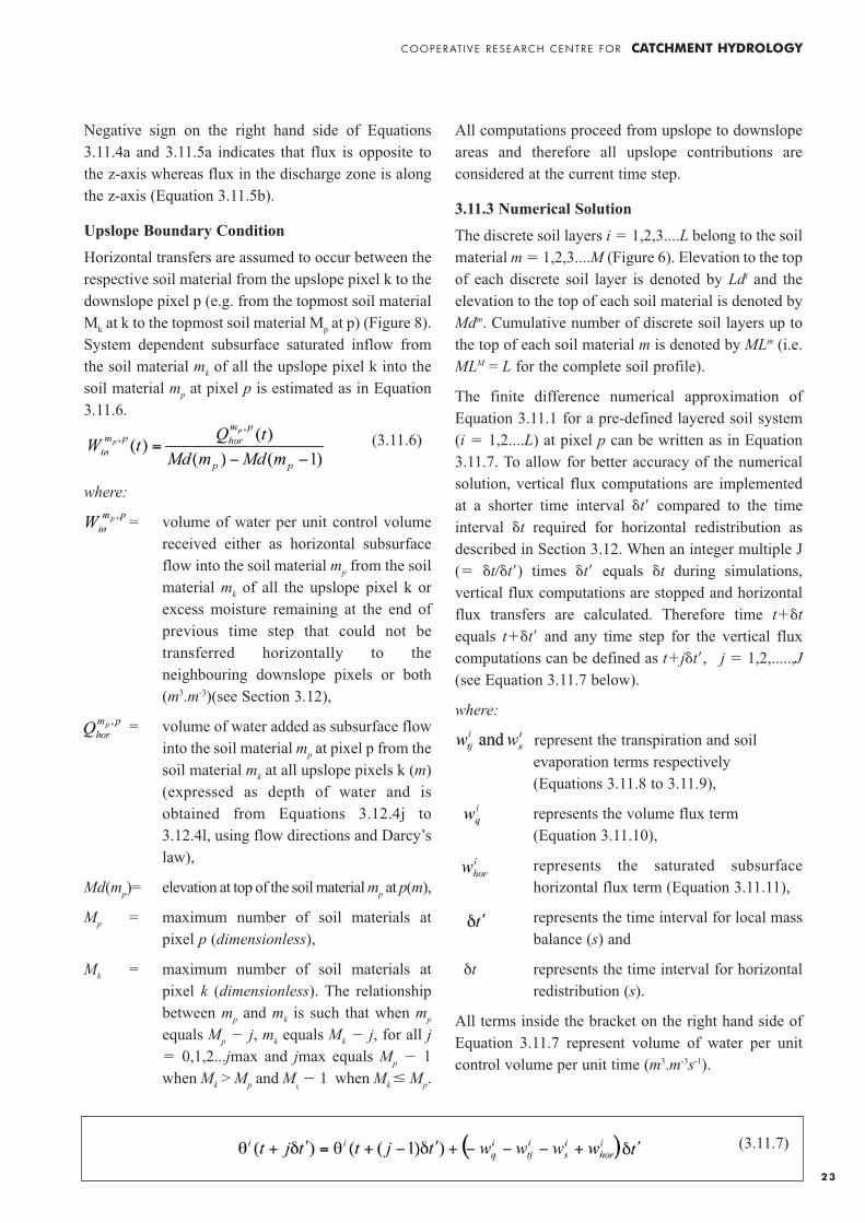
Horizontal transfers are assumed to occur between therespective soil material from the upslope pixel k to thedownslope pixel p (e.g. from the topmost soil materialMk at k to the topmost soil material Mp at p) (Figure 8).System dependent subsurface saturated inflow fromthe soil material mk of all the upslope pixel k into thesoil material mp at pixel p is estimated as in Equation3.11.6.

(3.11.6)

where:

= volume of water per unit control volumereceived either as horizontal subsurfaceflow into the soil material mp from the soilmaterial mk of all the upslope pixel k orexcess moisture remaining at the end ofprevious time step that could not betransferred horizontally to theneighbouring downslope pixels or both(m3.m-3)(see Section 3.12),

= volume of water added as subsurface flowinto the soil material mp at pixel p from thesoil material mk at all upslope pixels k (m)(expressed as depth of water and isobtained from Equations 3.12.4j to3.12.4l, using flow directions and Darcy’slaw),

Md(mp)= elevation at top of the soil material mp at p(m),

Mp = maximum number of soil materials atpixel p (dimensionless),

Mk = maximum number of soil materials atpixel k (dimensionless). The relationshipbetween mp and mk is such that when mp

equals Mp � j, mk equals Mk � j, for all j 0,1,2...jmax and jmax equals Mp � 1when Mk > Mp and M

k� 1 when Mk Mp.

All computations proceed from upslope to downslopeareas and therefore all upslope contributions areconsidered at the current time step.

3.11.3 Numerical Solution

The discrete soil layers i 1,2,3....L belong to the soilmaterial m 1,2,3....M (Figure 6). Elevation to the topof each discrete soil layer is denoted by Ldi and theelevation to the top of each soil material is denoted byMdm. Cumulative number of discrete soil layers up tothe top of each soil material m is denoted by MLm (i.e.MLM = L for the complete soil profile).

The finite difference numerical approximation ofEquation 3.11.1 for a pre-defined layered soil system(i 1,2....L) at pixel p can be written as in Equation3.11.7. To allow for better accuracy of the numericalsolution, vertical flux computations are implementedat a shorter time interval �t� compared to the timeinterval �t required for horizontal redistribution asdescribed in Section 3.12. When an integer multiple J( �t��t�) times �t� equals �t during simulations,vertical flux computations are stopped and horizontalflux transfers are calculated. Therefore time t��tequals t��t� and any time step for the vertical fluxcomputations can be defined as t�j�t�, j 1,2,.....,J(see Equation 3.11.7 below).

where:

represent the transpiration and soilevaporation terms respectively(Equations 3.11.8 to 3.11.9),

represents the volume flux term(Equation 3.11.10),

represents the saturated subsurfacehorizontal flux term (Equation 3.11.11),

represents the time interval for local massbalance (s) and

δt represents the time interval for horizontalredistribution (s).

All terms inside the bracket on the right hand side ofEquation 3.11.7 represent volume of water per unitcontrol volume per unit time (m3.m-3s-1).

(3.11.7)


2 4

(3.11.8)

(3.11.9)

(3.11.10)

(3.11.11)

where:

L = total number of the discrete soil layers,

= canopy transpiration demand over thetime step t + �t obtained from Equation3.7.1 (m.s-1),

= soil evaporation demand over the timestep t � �t obtained from Equation 3.7.1(m.s-1),

= volume of water per unit control volumereceived as inflow over the time stepδt�(m3.m-3),

= number of time steps for the vertical massbalance within a single time step forhorizontal redistribution (-).

Plant transpiration demand from the canopy andthe soil evaporation demand Es are available fromclimate forcing for the time t � δt (3.7.1).Computations for a given pixel p are performed onlyafter computations for all the upslope pixels thatcontribute to p are completed. Therefore volume ofwater added to pixel p as horizontal saturated flow

from all the upslope pixels k, isavailable from Equation 3.11.6 at the end of currenttime step of the horizontal transfers (Equation 3.11.11).

Ideally spatial derivative of the Darcy’s flux alongthe vertical should be considered at time

i.e. implicit solution of the Richard’sequation. However, for a catchment based modellingsystem, computational requirements would be toomuch. Therefore, the term is considered at time

(Equations 3.11.12 to 3.11.13) i.e.explicit solution of Equation 3.11.7. When the timestep for the vertical water balance is small relativeto the horizontal re-distribution time step δt, thesolution approaches the implicit solution of Equation3.11.1 and the numerical simulation times are likely tobe large.

Moisture contents are considered at the node.Hydraulic conductivity and diffusivity are consideredat the interface of the adjoining discrete soil layers andare expressed as geometric mean of the respectivevalues (see Equations 3.11.12 and 3.11.13 below).

where:

= infiltration from the soil surface fromEquation 3.11.4a (m.s-1),

= flux from bottom of the soil profile overthe time step from Equations3.11.5a to 3.11.5b (m.s-1).

(3.11.12)

(3.11.13)


2 5

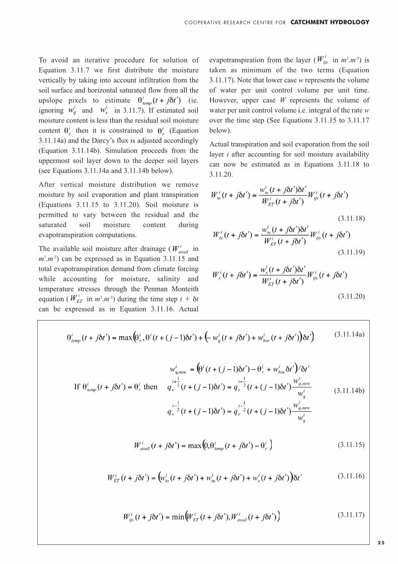
To avoid an iterative procedure for solution ofEquation 3.11.7 we first distribute the moisturevertically by taking into account infiltration from thesoil surface and horizontal saturated flow from all theupslope pixels to estimate (ie.ignoring and in 3.11.7). If estimated soilmoisture content is less than the residual soil moisturecontent then it is constrained to (Equation3.11.14a) and the Darcy’s flux is adjusted accordingly(Equation 3.11.14b). Simulation proceeds from theuppermost soil layer down to the deeper soil layers(see Equations 3.11.14a and 3.11.14b below).

After vertical moisture distribution we removemoisture by soil evaporation and plant transpiration(Equations 3.11.15 to 3.11.20). Soil moisture ispermitted to vary between the residual and thesaturated soil moisture content duringevapotranspiration computations.

The available soil moisture after drainage ( inm3.m-3) can be expressed as in Equation 3.11.15 andtotal evapotranspiration demand from climate forcingwhile accounting for moisture, salinity andtemperature stresses through the Penman Monteithequation ( in m3.m-3) during the time step t � δtcan be expressed as in Equation 3.11.16. Actual

evapotranspiration from the layer ( in m3.m-3) istaken as minimum of the two terms (Equation3.11.17). Note that lower case w represents the volumeof water per unit control volume per unit time.However, upper case W represents the volume ofwater per unit control volume i.e. integral of the rate wover the time step (See Equations 3.11.15 to 3.11.17below).

Actual transpiration and soil evaporation from the soillayer i after accounting for soil moisture availabilitycan now be estimated as in Equations 3.11.18 to3.11.20.

(3.11.18)

(3.11.19)

(3.11.20)

(3.11.14a)

(3.11.14b)

(3.11.15)

(3.11.16)

(3.11.17)


2 6

When equals , evapotranspiration demandestimated from Penman Monteith equation iscompletely satisfied (atmospheric control). However,when is less than , moisture availabilitydetermines the evapotranspiration amounts (soilcontrol). Soil moisture is then adjusted depending onwater loss by evapotranspiration (Equation 3.11.21). Ifthe estimated soil moisture content for any soil layer isgreater than the saturated soil moisture content then it is constrained to the saturated soil moisturecontent and excess moisture is computed (Equation3.11.22).

Total transpiration, soil evaporation and excessmoisture is then accumulated for each soil layer overthe horizontal transfer time step δt as in Equation3.11.23.

(3.11.23)

Drainage from the soil profile and flux across thebottom of each soil material is accumulated over thetime step t � δt as in Equation 3.11.24.

where:

= flux at the bottom of the soilmaterial mp at p over the horizontalre-distribution time step (m).

Flux across the top of each soil material is accumulatedover the time step t � δt as in Equation 3.11.25.

where:

= flux across the top of the soilmaterial mp at p over the horizontalre-distribution time step (m).

3.12 Horizontal Redistribution and Sub-surface Flow from each Soil material

Soil moisture in excess of the moisture holdingcapacity for each discrete soil layer is accumulatedover the respective soil material and is transferred assub-surface flow to the two downslope pixelsaccording to the multiple flow direction algorithm ofTarboton (1997) and Darcy’s law. Horizontal transfersoccur over the time interval δt.

The sub-surface flow routing model is adapted from agrid based quasi three-dimensional model ofWigmosta and Lettenmaier (1997). An importantdifference between the approach of these authors andthe popularly used statistical dynamical approachoriginally proposed by Beven and Kirkby (1979) is theuse of grid cells as against the use of hydrologicalsimilarity concepts. The hydrological similarityconcept or the wetness index, while numerically verysimple, is not suitable for predicting the effects oflanduse change which is the primary objective ofCLASS. For practical reasons landuse changes areinvariably required at the property level and theobjective is not to just predict the impact of landusechanges at the catchment outlet but also to quantify thedownslope landscape impacts. Many differentlandscape elements in the catchment can have samewetness index. This produces difficulties inimplementing landuse change scenarios.

(3.11.24)

(3.11.25)

(3.11.21)

(3.11.22)


2 7

The excess moisture content fromEquation 3.11.23 of the discrete soil layers is pooledover the respective soil material depth to estimate thetotal excess moisture over the soil material (Equation3.12.1). Material soil moisture is then estimated(Equation 3.12.2). A perched water table is createdseparately for each material when proportional soilmoisture becomes unity (Equation 3.12.3).

Total excess soil moisture in each soil material mp at pcan be estimated as depth of water as in Equation 3.12.1.

(3.12.1)

where:

= moisture in excess of saturated moisture-holding capacity in the soil material mp

(m).

Soil moisture over the soil material (m3.m-3) and theproportional soil material saturation (dimensionless) are estimated as in Equations 3.12.2and 3.12.3 respectively.

(3.12.2)

(3.12.3)

Letting nd denote the number of downslope pixels k,k 0,1,2,....,7 with non-zero flow weight (δpk � 0), itsvalue equals 1 for the D8 method and equals either 1or 2 for the D∞ method (Tarboton, 1997). The soilmaterials 1,2,.....,Mp at pixel p and 1,2,.....,Mk at k arenumbered from the bottom (Figure 6). Saturatedhorizontal transfers are permitted between therespective soil materials from the top i.e. Mp to Mk, Mp

�1 to Mk �1 etc. Since the number of soil materialsMp at p and Mk at k can be different, therefore mapping

of a given soil material mp at p to the respective soilmaterial mk at k is required as in (3.12.4a).

(3.12.4a)

For each downslope pixel k with non-zero flow weight(1,2,...,nd), calculate the available soil moisture forhorizontal transfer from soil material mp at p to therespective soil material mk at k (Equation 3.12.4b) andalso from Darcy’s law (Equations 3.12.4c to 3.12.4i).

(3.12.4b)

(3.12.4c)

(3.12.4d)

(3.12.4e)

(3.12.4f)

(3.12.4g)

(See Equations 3.12.4h and 3.12.4i below)

where:

= moisture available for horizontal transferfrom the soil material mp at p to therespective soil material mk at k (m),

= moisture that can be transferredhorizontally using Darcy’s law from thesoil material mp at p to the respective soilmaterial mk at k (m),

= soil moisture (m3.m-3),

KH=KV /IKA

= unsaturated hydraulic conductivity alongthe horizontal axis (m.s-1),

IKA = anisotropy ratio (-),

(3.12.4h)

(3.12.4i)


2 8

h = pressure head (m),

= difference between moisture available forhorizontal transfer and moisture that canbe transferred from soil material mp at p tothe respective soil material mk at k (m),

= distance between the centre of pixel p andk (m).

A lower bound is introduced in Equation 3.12.4h toensure that excess moisture gets to the streameventually in the areas of low relief.

The variable can take a positive, negative or azero value (Equation 3.12.4i). A positive valueindicates that Darcy’s flux is the limiting case whereasa negative value indicates that moisture availability isthe limiting case. A zero value indicates balancebetween the available moisture and the moisture thatcan be transferred from the soil material mp at p to therespective soil material mk at k.

Case 1

For each downslope pixel k with non-zero flow weight(nd pixels with �pk�0) that have , calculateactual horizontal soil moisture transfer from mp at p tomk at k using Equation 3.12.4j. Maintain a record of allinflow coming into the soil material mk at k anddepletion of the excess moisture from the soil materialmp at p (see Equation 3.12.4j below).

where:

= actual horizontal soil moisture transferfrom the soil material mp at p to mk at k(m),

= inflow coming into the soil material mk at pixel k from all neighbouring upslope pixels with δpk >0(m),

= total horizontal outflow from the soil material mp at p to the neighbouring downslope pixels during the time step t � δt (m).

Case 2

For each downslope pixel k with non-zero flow weight(nd pixels with δpk > 0) that have ,calculate actual horizontal soil moisture transfer frommp at p to mk at k using Equation 3.12.4k. Equation3.12.4k can be applied ONLY so long as some excesssoil moisture is available for horizontal transfer

(see Equation 3.12.4k below).

If solute transport is simulated, Equations 4.1.7 to4.1.8 must be estimated after estimating Equations3.12.4j to 3.12.4k.

If some excess moisture is still available in the soilmaterial mp at p after performing(Equations 3.12.4j to 3.12.4k), then this moisture ismade available for vertical drainage andevapotranspiration at the next time step (Equation3.12.4l) (see upslope boundary condition Equation3.11.6). This step should be performed just beforecomputation for this pixel is finished.

(3.12.4l)

(3.12.4j)

(3.12.4k)


2 9

In computing Equations 3.12.4a to 3.12.4k, horizontaltransfer of excess moisture is done for the first soilmaterial (mp 1) at p to all downslope pixels k (nd

pixels with �pk�0). Thereafter soil materials are takenup sequentially (Equations 3.12.4a to 3.12.k) andcomputations are performed.

3.13 Soil Material Water Balance

A material water balance for pixel p is conducted byexpressing all fluxes over the time step and soilmoisture storage as depth of water (m).

Actual soil evaporation and the overstory andunderstory plant transpiration over each soil materialare estimated using Equations 3.13.1 to 3.13.2respectively.

(3.13.1)

(3.13.2)

where:

= actual soil evaporation from the soilmaterial mp (m),

= actual transpiration from the soil materialmp and canopy j (m).

Total horizontal inflow to the soil material and outflowfrom the soil material is estimated as in Equations3.13.3 and 3.13.4 respectively.

(3.13.3)

(3.13.4)

where:

= total horizontal saturated subsurfaceinflow into the material mp during the timestep (obtained from upslope areas at the

beginning of current time step)(m)(Equations 3.12.4j to 3.12.4k),

= total horizontal saturated subsurface outflowfrom the material mp during the currenttime step (m) (Equations 3.12.4j to 3.12.4k).

Total vertical flow (m) from bottom of the soilmaterial and (m) from top of the soil materialare estimated from Equations 3.11.24 and 3.11.25respectively.

Actual available soil moisture storage for eachmaterial Smp

(m) is obtained from Equations 3.13.5 to3.13.6.

(3.13.5)

(3.13.6a)

(3.13.6b)

where:

= proportional soil moisture saturation(-).

Estimated soil moisture storage and proportional waterbalance error are estimated from Equations 3.13.7 and3.13.8 respectively. The variable includes excess water generated during the verticalwater balance that could not be transferredhorizontally after horizontal redistribution.Cumulative water balance error for each soil materialis estimated using Equation 3.13.9.

(3.13.8)

(3.13.9)

(3.13.7)


3 0

where:

= proportional water balance errorduring the time step (-),

= Cumulative proportional waterbalance error up to the end of currenttime step (-).

3.14 Generated Surface Runoff, GroundwaterRunoff and Runoff Routing

A schematic diagram illustrating partitioning of thewater balance components on three pixels along asingle hillslope is shown in Figure 9. Typical range ofthe water balance fluxes under dryland conditions inNSW for pasture, trees and cropping are also shown.

3.14.1 Generated Surface Runoff

Overland flow and saturated horizontal sub-surfaceflow are transferred within the landscape usingmultiple flow path algorithm of Tarboton (1997) andDarcy’s law. The method accounts for advective fluxalong the flow path that is determined by topographyand accounts for travel times along these flow paths.

Generated surface runoff comprising overland flowand shallow sub-surface flow at each pixel on thestream ps is added to get the total generated surfacerunoff as in Equation 3.14.1. Shallow sub-surface flowis defined as the horizontal sub-surface flow from allsoil materials.

(3.14.1)

where:

= total generated surface runoff over thetime step t + δt at all pixels ps on thestream (m),

Ps = total number of pixels in the catchmentlocated on the stream (-),

= horizontal sub-surface flow over the timestep t + δt received at soil material mp atpixel ps on the stream (m) (from Equations3.12.4j to 3.12.4k),

Figure 9. Schematic Diagram of Partitioning of the Water Balance Components and Simulated Landuse:- (a) rainfall,(b) crops, (c) trees, (d) pasture, (e) evapotranspiration, (f) overland flow, (g) shallow sub-surface flow, (h)drainage from the modelled soil profile, (i) lateral throughflow, (j) recharge to the Groundwater Flow System(GFS), (k) discharge from the GFS to the land (l) and to the stream (m), and (n) recharge to the regionalsystem.


3 1

= overland flow received over the time stept + δt at pixel p from the upslope pixels(m) (from Equation 3.11.4f).

3.14.2 Generated Groundwater Runoff and Lateral Throughflow

The catchment can be divided into a number ofGroundwater Flow Systems (GFS) and such spatialdata are available on a widespread basis in Australia.Metadata associated with each GFS contains thehydrogeological information ie. conductivity,transmissivity, specific yield and depth of the aquiferetc. Therefore location of each pixel within a givenGFS is known from the spatial GFS datasets.

Moisture content of the deepest soil layertakes into account drainage from thesoil profile according to Equations 3.11.5a to 3.11.5busing the lower boundary condition for each pixel pwithin a given GFS (Figure 9: h). A proportion of thisdrainage reaches the groundwater flow system (GFS)(Figure 9:j) from where it leaves the catchment eitheras discharge to stream or land or both (Figure 9:k). Theremaining proportion of the drainage that cannot enterthe GFS is discharged either to the land or to thestream or both through deeper sub-soil as lateralthroughflow (Figure 9:i). Partitioning of the deepdrainage into recharge to the GFS (Equation 3.14.2)and lateral throughflow can be obtained usingconductivity of the sub-soil and the GFS (Equation3.14.3).

(3.14.2)

(3.14.3)

where:

= deep drainage from bottom of themodelled soil profile at pixel p within ith

groundwater flow system GFSi (m)(Equation 3.11.24),

= recharge from pixel p to the GFSi (m),

= lateral throughflow from pixel p over theGFSi (m),

= saturated hydraulic conductivity of theGFSi where pixel p is located (m.s-1),

= saturated hydraulic conductivity of thesub-soil at pixel p (m.s-1).

The spatial distribution of the depth of soil can bepredicted using the methodology of McKenzie etal.,(2003) (Section 3.2.2). This information on totalsoil depth (HSD) can be used to estimate the verticaldistance between depth of soil from bottom of themodelled soil profile (Md 0) and the geology of theGFS. Using this vertical distance with the conductivityof the sub-soil, travel time along the vertical to thebottom of the soil profile can be estimated (Equation3.14.4).

(3.14.4)

where:

= travel time at pixel p along the verticalfrom bottom of the modelled soil profileto top of the geology (s),

= depth of soil at pixel p from surface to topof the geology (m),

Z p = elevation of the soil surface at pixel p wrtmean sea level (m),

Md 0,p = elevation of the bottom of the modelledsoil profile at pixel p (m),

= saturated hydraulic conductivity of thesub-soil at pixel p (m.s-1).

Typically average slope length in the drylandcatchments across NSW varies in the range 175-250 m.FLAG landform at every pixel location is available(Section 3.2.1). This information can be used toestimate representative length of the landform (in plan) between the pixel location within a givenFLAG landform and the discharge area. Using this(horizontal) length with the hydraulic conductivity ofthe GFS/sub-soil, horizontal travel time from the GFSor sub-soil to the discharge area can be estimated(Equations 3.14.5a to 3.14.5b). If flow path frombottom of the modelled soil profile to the GFS isvertical and along the GFS is horizontal, thenmaximum travel time is sum of the vertical and


3 2

horizontal travel times. However, the resultant flowpath is likely to be somewhat shorter and therefore ascaler is introduced in Equations 3.14.6a to 3.14.6b. Itis pointed out that modelling of preferential flowcomponent is not included in CLASS.

(3.14.5a)

(3.14.5b)

(3.14.6a)

(3.14.6b)

where:

= average representative slope length of theFLAG landform at pixel p from bottom ofthe discharge area (m),

LC = confining upslope length from the streamwhere the aquifer behaves as aconfined/semi-confined (m),

KGFSi = saturated hydraulic conductivity of theGFSi on which pixel p is located (m.s-1),

= saturated hydraulic conductivity of thesub-soil on which pixel p is located (m.s-1),

= travel time along the horizontal within theGFSi on which pixel p is located (s),

= travel time along the horizontal within thesub-soil on which pixel p is located (s),

= total travel time from bottom of themodelled soil profile through the sub-soiland the GFS to the discharge area (s),

= total travel time from bottom of themodelled soil profile through the sub-soilto the discharge area (s),

= scaler representing ratio of the resultant

flow path and the longest flow path ( 1)(-).

The confining upslope length LC is introduced inEquation 3.14.5a because pressure signal in theconfined system is assumed to be much faster than thephreatic system.

Drainage from bottom of the soil profile needs to belagged to allow for water to reach discharge areas onthe land and the stream. Lagged recharge and lateralthroughflow for each pixel p are estimated as inEquations 3.14.7 to 3.14.8.

(3.14.7)

(3.14.8)

where:

= time lag through the sub-soil (vertical)and the GFS (horizontal) (s),

= time lag through the sub-soil (vertical)and the sub-soil overlying the GFS(horizontal) (s).

Total discharge and lateral throughflow can beestimated by accumulating lagged recharge from allpixels p within a given GFSi (Equations 3.14.9 to3.14.10).

where:

= total discharge to the land and to thestream from a given GFSi (m),

= total lateral throughflow to the land and tothe stream from all pixels in a given GFSi (m),

LGFSi = leakage to the GFSi to the regionalgroundwater system (-) ( ).

Discharge from the GFS is partitioned into streamdischarge and land discharge as in Equations 3.14.11to 3.14.12.

(3.14.9)

(3.14.10)


3 3

(3.14.11)

(3.14.12)

where:

= lagged discharge from GFSi (m),

= lagged discharge from GFSi to theland (m),

= lagged discharge from GFSi to thestream (m),

= partitioning coefficient of thedischarge to land ( ;from Equation 3.14.15) (-),

= lagged time (s).

Lateral throughflow from deep sub-soil over each GFSis partitioned into stream discharge and land dischargeas in Equations 3.14.13 to 3.14.14.

(3.14.13)

(3.14.14)

where:

= lagged lateral throughflow fromGFSi (m),

= lagged lateral throughflow fromGFSi to the land (m),

= lagged lateral throughflow fromGFSi to the stream (m),

= lagged time (s).

The partitioning coefficient L of discharge from agiven GFSi to the land is obtained as in Equation 3.14.15.

(3.14.15)

where:

AL = land area in the catchment affected byshallow water table (obtained frommapped discharge areas on land and theFLAG model) (m2),

ASApPsas

= area of stream in the complete catchment(m2),

Ap = area of the pixel (m2),

Ps = total number of pixels on the stream in thecatchment (-),

as = average proportion of the pixel areaoccupied by the stream (-),

�L = discharge weighting to land relative to thestream (-),

�S = discharge weighting to stream relative toitself (equal to 1)(-).

Total generated groundwater discharge to the streamand land from all the groundwater flow systems cannow be estimated as in Equations 3.14.16 to 3.14.17.

(3.14.16)

(3.14.17)

where: = total groundwater discharge to the stream(m),

= total groundwater discharge to the land(m),

NGFS = total number of groundwater flow systemsin the catchment (-).

Average upward flux for each pixel p in the dischargearea on the land is estimated as Equation 3.14.18.

(3.14.18)

where:

Pdisch = number of pixels in discharge areas in thecatchment (-),

= average upward flux from bottom of themodelled soil profile of pixels in thedischarge areas at time (m.s-1),

�t = time interval of the horizontal re-distribution (s).


3 4

3.14.3 Surface Runoff Routing

Generated surface runoff component includes shallowsubsurface and the overland flow components andaccounts for travel time along the hillslope. Generatedsurface runoff (rs) and the routed surface runoff (Qs)represent time-averaged values over the time step t +δt. Surface runoff generated at all the pixels on thestream (from Equation 3.14.1) is routed along thestream (attenuation and lag) to the catchment outletusing the linear cascade model of Nash (1960) as inKachroo and Liang (1992). Nash model is based onthe assumption that storage in the system varieslinearly with discharge from the system. Using thisassumption with the differential equation describingclassical mass balance, Nash (1960) obtained thegeneral solution relating a given input of unit volumeto a given output as in Equation 3.14.2.

(3.14.19a)

(3.14.19b)

where:

�t = simulation time interval (s),

τ = time (s),

K1 = K2 = …… = Kn = K are the storage coefficientsof n linear reservoirs in cascade(units of �t),

h(t + �t) = ordinates of the pulse responsefunction (units of δt -1) and T(n)incomplete Gamma function(dimensionless).

It was shown by Nash (1960), that under constraints ofconservation, stability, high damping and the absenceof feedback, this two-parameter equation with n aninteger and K positive, is almost as general a model asthe differential equation of unlimited order. Withadditional flexibility obtained by allowing n to takefractional values, the impulse response of thisequation has the ability to represent, adequately,almost all shapes commonly encountered in thehydrological context.

The assumption of linearity is largely valid and theapproach works reasonably well for time scale inhours or days. However non-linear effects arepronounced when time scale and stream length issmall, and the technique is less effective in describingthe input-output relationship.

The linear model described by Equation 3.14.19 is thesimplest representation of a causal, time-invariant,relationship between an input function of time(generated surface runoff) and the correspondingoutput function (routed surface runoff). It is used as acomponent representing the routing or diffusioneffects of the catchment on those components of thegenerated streamflow contributing to the catchmentoutflow (Equation 3.14.20).

(3.14.20)

where:

m� = memory of the pulse response function(units of δt).

The parameter pair n and nK are chosen foroptimisation, rather than n and K separately, because nis a ‘shape’ parameter and nK is the ‘scale’ parameter.Expressed in this way, the two parameters are likely tobe more independent than n and K would beseparately, both of which contribute to the scale and tothe shape, although in different ways.

3.14.4 Groundwater Routing

Total generated groundwater discharge fromlandscape to the stream Qg(T�) is routed using similarapproach as the surface runoff (Equations 3.14.19 to3.14.20) but with separate parameters ng and ngKg.


3 5

4. CLASS Solute Balance Components

A solute balance is conducted for each soil material ateach pixel following water balance computations oneach day.

4.1 Determining Discharge Areas in a Catchment

Water logged areas in a catchment can be determinedusing either mapped areas with shallow water table orfrom the Fuzzy Landscape Analysis GIS FLAG model(Roberts et al., 1997) or both. Salt outbreak maps forlarge areas in New South Wales (NSW) are available.Also the outputs of the FLAG model are available forthe whole state (Summerell et al., 2003a,b). In the caseof salinity, these maps are used in conjunction with thegeology maps as a basis for describing initial salinityconditions across the catchment (Murphy et al., 2003).

Fuzzy Landscape Analysis GIS (FLAG) uses griddedelevation data to calculate the wetness of soils. Thismodel categorises grid cells based on their position inthe landscape. These categories are then used to inferthe landscape processes associated with their wetnessand location.

FLAG uses three measures – WET-REGION, WET-LOCAL and WET-LU to derive soil wetness. For thisapplication modelling was done at the catchment scaleof 600-3000 km2. WET-REGION is the relative heightof each cell overall in the landscape, which is anindirect measure of the amount of surface and sub-surface water accumulation. As WET-REGIONincreases the volume of water entering a cell increases.WET-LOCAL is a measure of local lowness for apredefined area around each cell. As WET-LOCALincreases, low areas where water tables are likely to benearer the surface are highlighted. The overall wetnessindicator which uses both WET-REGION and WET-LOCAL is called WET-LU.

Combining the spatial indicator values within a GISframework enables maps of wetness hazard to bedrawn at scale of paddocks, catchments and basins.

The FLAG approach thus derives scaled indicators asrelative measures, and can be considered as the firstiteration to guide or complement more detailed studiesof changes to the water cycle, including salinisationand water logging.

4.2 Current In-stream Solute Export Model

Solute concentration time series is required as a basedata set to calibrate the solute transported fromlandscape to the stream. In the case of salts, streamsalinity measurements for catchments in NSW startedon a large scale in early 1970s. Few of the sites containcontinuous measured data while most sites havemonthly or fortnightly measurements. For catchmentswhere continuous salinity data are available, these canbe used for calibrating salt output from thecatchments. However, there are many catchments inNSW where long-term salt export rates are requiredbut the available salinity data are either for a shortperiod or are patchy. In such instances, a daily salt loadtime series can be created using an objectivemethodology based on stochastic hydrology concepts(Beale et al., 2000; Tuteja et al., 2000).

4.3 Solute Mass Balance over the Soil Material

Miscible displacement of solutes across the landscapeinvolves three transport mechanisms, namely,advection, molecular diffusion and hydrodynamicdispersion. Dispersive and diffusive solute fluxes(hydrodynamic dispersion) that result in solutespreading in horizontal directions are neglected in thecurrent version. Solute spreading in CLASS occursfrom spreading of water down the hillslope which inturn results from multiple flow directions (Tarboton,1997). Solute transfer between a pixel and itsneighbours occurs with the respective soil materials.

Solute balance equations are written for each soilmaterial at pixel p in the liquid and the solid phase asin Equations 4.3.1 and 4.3.2 respectively.

(4.3.1)


3 6

where:

= solute mass at p and soil material mp (kg),

= solute mass at p entering from top of thesoil material mp (kg),

= solute mass at p leaving from bottom ofthe soil material (kg),

= solute mass at p precipitated from theoverstory and understory transpirationand the soil evaporation processesrespectively (kg),

= solute mass entering (leaving) the soilmaterial mp at p horizontally from upslope(to downslope) pixels (kg),

= solute mass dissolved from the soilmaterial mp at p (dissolved and adsorbedsolutes are considered in equilibrium) ( kg),

= first order rate of decay (s-1),

= solute concentration adsorbed to the soil (kg).

The solute mass terms , , , and are obtained by multiplying the

water flux terms in Equations 3.11.24 to 3.11.25 andEquations 3.13.1 to 3.13.6 with the respective solute

concentration and area of the pixel. Denotingconcentration of the solute in liquid and solid phase asCw (kg.m-3) and Cs (g.kg-1) respectively, these terms areexpressed as in Equations 4.3.3 to 4.3.6.

(4.3.3)

(4.3.4)

(4.3.5b)

(4.3.6b)

where:

A = area of the pixel (m2),

= solute concentration of the GFSi wherepixel p is located (kg.m-3).

The condition can occur only if pixel p islocated in the discharge area. The horizontal soluteoutflow from the soil material mp is estimated usingEquations 4.3.7 to 4.3.8. If solute transport issimulated, this step must be performed whenEquations 3.12.4j to 3.12.4k are computed (seeEquation 4.3.7 and Equation 4.3.8).

(4.3.2)

(4.3.5a)

(4.3.6a)

(4.3.7)

(4.3.8)


3 7

where:

= saturated sub-surface flow from the soilmaterial mp at pixel p to a neighbouringdownslope pixel k (m) (from Equations3.12.4j to 3.12.4k). The relationshipbetween mp and mk is described byEquation 3.12.4a.

The Freundlich isotherm describing equilibriumexchange between dissolved and adsorbed soluteconcentration can be used as in Equation 4.3.9.

(4.3.9)

where:

KF and F are the parameters.

Solute mass dissolved from the soil material mp at p(solute desorbed under equilibrium exchange) can be estimated using Equation 4.3.10.

where:

= soil moisture in the soil material mp at p(m) (from Equation 3.13.8 at previoustime step),

= proportion soil material saturation or thespecific saturation (dimensionless) (fromEquation 3.13.6b). Specific saturation isincluded in Equation 4.3.10 becausedissolution occurs through moisture andmatrix contact surface.

Solute concentration in liquid and solid phase can beestimated as in Equations 4.3.11 and 4.3.12respectively.

(4.3.11)

(4.3.12)

where:

= solute concentration in liquid phase (kg.m-3),

= solute concentration in solid phase (g.kg-1),

= bulk density of the soil material mp at p(kg.m-3).

4.4 Solute Transport in the Stream

Surface runoff includes shallow subsurface and theoverland flow components. All the solute reaching thepixel ps defined as a stream node is pooled together asgenerated solute mass. The solute reaching the streamnode with the lateral throughflow is also added to thestream (Equation 4.3.7). Recharge to the groundwatersystem is pooled separately for the GFS and therespective solute concentration is used to estimate thesolute flux into the stream with groundwaterdischarge.

The generated solute mass is routed to the catchmentoutlet with the routed runoff and the assumption offully mixed flow.

(4.3.10)


3 8


3 9

5. Time Stepping

User specified time steps are used for vertical andhorizontal flux computations. Vertical fluxcomputations for solution of the Richard’s equationcan be obtained at a sub-daily time step and allhorizontal transfers are performed at a larger time step.It is assumed that the time step for horizontal transferswould be an integer multiple of the shorter time stepused for vertical flux computations. All pasture andcrop growth simulations are performed at a daily timestep while all tree growth computations are performedat a monthly time step.


4 0


4 1

6. Data Requirements and Model Parameters

Data requirements for CLASS are described in thissection. Parameters required by the CLASSHydrology models U3M-1D (Vaze et al., 2004), U3M-2D (Tuteja et al., in prep.a) and CLASS CatchmentModel (Tuteja et al., in prep.c) are described in therespective User’s Manual. Likewise, respective User’sManual of the models CLASS PGM, CGM and 3PG+describe the parameters required for plant growthmodelling (Vaze et al., 2004a, Vaze et al., 2004b;Tuteja et al., in prep.b). Parameters required for spatialdata relating to soil depth are described in the CLASSSpatial Analyst User’s Manual (Teng et al.,2004).

6.1 Spatial Data Requirements

Climate data: Maximum and minimum airtemperature (ºC), rainfall (mm/d), pan evaporation(mm/d), shortwave radiation (MJ.m-2), vapourpressure (hPa), maximum and minimum relativehumidity (%). These data are available from SILOdatabase (Jeffrey et al., 2001). CLASS Spatial Analystaccepts gridded data and performs climate zoningbased on user specified climate zones.

DEM: Digital elevation model of any resolution.Normally, 25 m DEMs are widely used in Australia.Depending on the catchment size, the problem sizemay be too large. In such instances, the CLASSSpatial Analyst can coarsen the DEM in multiples of25m, and all spatial data required by CLASS areadjusted accordingly.

FLAG upness index: Spatial data for the FLAGupness index are available for the whole of NSW(Summerell et al., 2003a). Alternatively, if these dataare not available, then it can be obtained using theFLAG model (Roberts et al., 1997).

MRVBF Index: Spatial data for the MRVBF Index(Gallant and Dowling, 2003). If these data are notavailable, then it can be obtained using thefunctionality available in the CRCCH TIMEenvironment (Rahman et al., 2003).

Landuse: DIPNR landuse maps for the catchment,and/or the Australian Landuse Classification System –ALCC (Barson et al., 2000; Stewart et al., 2001).

GFS: Spatial data for the Groundwater flow systemsand the associated metadata on solute concentration,hydraulic conductivity, transmissivity, specific yieldand depth of aquifer. In NSW, such data are generallyheld in Regional databases.

Soils: Spatial data for distribution of soils. In NSW,these data are obtained using Murphy et al.,(2003)methodology.

Soil salinity: Spatial data for distribution of soilsalinity. In NSW, these data are obtained usingMurphy et al.,(2003) methodology. Input EC1:5 dataunits are in dS/m and model converts it into grams ofcontaminant per kilogram of soil.

6.2 Temporal Data Requirements

CLASS can be validated both in-stream as well as onthe inland landscape. In-stream data are required as aminimum calibration data set. Additionally, inlandlandscape data relating to hydrology and plant growthwould be helpful in increasing confidence in themodel predictions.

Streamflow data: Streamflow data (mm/d) timeseries at the catchment outlet. Additional data atgauging stations within the catchment would behelpful in the calibration exercise.

Water quality data: In-stream solute concentrationdata (kg.m-3) time series at the catchment outlet.Additional data at gauging stations within thecatchment would be helpful in the calibration exercise.

Soil hydrology data: Soil moisture data (m3.m-3) timeseries within the catchment.

Plant growth data: Plant growth data time serieswithin the catchment. Growth data includes LAI, stemand root biomass, groundcover etc.


4 2


4 3

7. Summary

The theoretical framework of a new distributed waterand solute transport model CLASS, currently underdevelopment is presented. The model is intended forimplementation on medium to large sized catchmentsto investigate the effects of landuse and climatevariability on catchment scale. Equations forcatchment scale investigation of water and solutetransport including the numerical solution andinteraction of the various components are detailed.The model is designed for Australian conditions anddata constraints often imposed in catchment scaleinvestigations have been taken care of in designingvarious components of the model. In particular themodel is adapted to spatial data and tools relating tosoils, topography and groundwater flow systemscommonly used in Australia.

Information on spatial distribution of soils and theirhydraulic properties is one of the most difficult datarequired in catchment scale modelling. Terrainanalysis indices from the FLAG model (Roberts et al.,1997; Summerell et al., 2003a-b) and MRVBF(Gallant and Dowling, 2003) are combined and used todescribe various landforms along the hillslopes. Theseare then combined with the soil landscape mappingand the geologies using the framework of Murphy etal.,(2003) to predict the spatial distribution of the soiltypes and soil physical properties. The properties ofthe soil types are identified from available soil surveydata and these properties are then translated into soilhydraulic properties using PTFs from Minasny andMcBratney (2002). The soil salinity properties arepredicted from the soil survey data.

The model includes comprehensive hydrology andgrowth components. The growth model includesannual and perennial pastures (C3 and C4) along with alegume, cropping and trees. The algorithms for thegrowth model are sourced from Johnson (2003).

Recharge and discharge areas are spatially defined a-priori as input using information on mapped areas ofshallow water table and the FLAG model. For eachpixel located in the catchment, water balance isperformed in the unsaturated zone along the verticalaxis using the Richard’s equation. A specified flux

boundary condition is used at the soil surface thatincludes atmospheric flux and overland flowcontribution from the upslope areas. The upslopeboundary condition includes horizontal sub-surfaceflow in each soil material from the respective soilmaterial from all neighbouring upslope pixels. A freedrainage boundary condition is used at the bottom ofthe modelled soil profile in the recharge areas. In thedischarge areas, an upward flux boundary condition isused at the bottom with flux estimated from landdischarge from upslope areas. When the landdischarge to the pixel in a discharge area is zero (dryconditions), a free drainage boundary condition isused at the bottom.

The vertical water balance in the unsaturated zone isperformed at a shorter time step relative to the timestep for horizontal transfers. Vertical fluxes at a givenpixel are accumulated over the horizontal time step.Moisture in excess of soil moisture holding capacity istransferred horizontally to the neighbouringdownslope pixels. Horizontal transfers occur betweenthe respective soil materials using the multiple flowpath algorithm of Tarboton (1997) and Darcy’s law.Horizontal transfers occur within the respective soilmaterials (eg. topsoil material of a given pixel to thetopsoil material of the neighbouring downslopepixels).

Drainage from the modelled soil profile is partitionedinto recharge to the underlying groundwater flowsystem (GFS) and lateral throughflow. Lateralthroughflow comprises water that cannot enter theaquifer and is transferred horizontally within the sub-soil to either the discharge areas on the land or to thestream or both. Recharge and lateral throughflow eachare pooled over the GFS. A proportion of each of thesecomponents is passed to the land as surface dischargeand the remaining component is passed to the stream.Discharge to the land is lagged appropriately and thenused as the upward flux boundary condition in thevertical water balance (upward flux boundarycondition). This time lag is based on the assumptionthat the bulk of the travel time results where the flowoccurs under phreatic conditions and that a fastpressure transmission signal applies in the confinedsystem.

Generated surface runoff comprising overland flow


4 4

and shallow sub-surface flow is pooled at all pixels onthe stream. Travel times along the hillslopes isaccounted for in horizontal transfers. Generatedsurface runoff and groundwater runoff, are routedusing the Nash model through separate responsefunctions to the catchment outlet.

Solute transport in the landscape accounts foradvection, but transport mechanisms associated withhydrodynamic dispersion are ignored. Solute transportin the stream includes solute sources from variouspathways and is routed to the catchment outlet withwater using the assumption of fully mixed flow.


4 5

8. Software Platform Related Issues

The CLASS modelling framework is developed on theMicrosoft.Net platform. The spatial components arewritten in VB.Net and currently operational onARCGIS8.3. Most of the aspatial model componentsare written in C#.Net. In 2004-05, the CLASSmodelling framework will be incorporated into ToolkitModelling Environment developed by the CooperativeResearch Centre for Catchment Hydrology (Rahmanet al., 2003).


4 6


4 7

11. References

Abbott, M. B., J. C. Bathurst, J. A Cunge., P. E.O’Connell, J. Rasmussen. 1986. An introduction to theEuropean hydrological system – systemehydrologique Europeen SHE, 1. History andphilosophy of a physically-based distributedmodelling system. Journal of Hydrology 87: 45-59.

Australian Bureau of Meteorology. 2001. ClimateAtlas of Australia: Evapotranspiration. Bureau ofMeteorology. ISBN 0642 320 489.

Band, L. E., P. Patterson, R. Nemani, and S. W.Running. 1993. Forest ecosystem processes at thewatershed scale: Incorporating hillslope hydrology.Agric. For. Meteorol. 63, 93-126.

Barson, M. M., L. A. Randall and V.L. Bordas, andCover Change in Australia. Results of thecollaborative Bureau of Rural Sciences - Stateagencies' Project on Remote Sensing of Land CoverChange. Bureau of Rural Sciences, Canberra, 2000.

Beer, T., 1990. Applied EnvironmetricsMeteorological Tables. Applied Environmetrics,Balwyn, Victoria, Australia, 56p.

Beven, K. J., M. J. Kirkby. 1979. A physically-basedvariable contributing area model of basin hydrology.Hydrological Science Bulletin 24: 43-69.

Beven, K., and J. Freer. 2001. A DynamicTOPMODEL. Hydrological Processes 15, 1993-2011.

Bronstert, A. 1995.User manual for the hillflow-3Dcatchment modelling system. Working document 95/4,CRC for Catchment Hydrology, Australia.

Brooks, R.H., and A.T. Corey. Properties of porousmedia affecting fluid flow, Journal of the Irrigation &Drainage Division 2 (June), American Society ofCivil Engineers, pp 61-88, 1966

Burman, R., and L.O. Pochop. 1994. Evaporation,evapotranspiration and climatic data. Elsevier,Amsterdam, 278p.

Burman, R., R.H. Cuenca, and A.Weiss. 1983.Techniques for estimating irrigation waterrequirements. In Hillel (1983), pp. 335-394.

Carsel, R.F., and R.S. Parrish, Developing jointprobability distributions of soil water retentioncharacteristics, Water Resources Research, 24: 755-769, 1988.

Costa-Cabral, M., and S. J. Burges. 1994. Digitalelevation model networks (DEMON): A model forflow over hillslope for computation of contributingand dispersal areas. Water Resources Research 30 (6):1681-1692.

Dawes, W., and T. Hatton. 1993. TOPOG_IRM 1.Model description, Technical memorandum 93/5,CSIRO Division of Water Resources, Australia.

Dickinson, R.E., A. Henderson-Sellers, C.Rosenzweig, and P. J. Sellers. 1991.Evapotranspiration models with canopy resistance foruse in climate models. A review, Agric. For. Meteorol.54, 373-388.

DLWC. 2000. The New South Wales Salinity Strategy– Taking on the Challenge. NSW Department of Landand Water Conservation, August 2000. ISBN 0 73475146 X

Dolezal, F. 2002. Report on outcomes of work, 5March-27 June 2002, unpublished data.

Dolezal, F. 1994. Physical Processes, Unpublishedlecture notes - International Post Graduate HydrologyCourse 1993-94, University College Galway, Ireland.

Dunin, F.X., E.M. O’Loughlin, W. Reyenga, 1988.Interception loss from Eucalypt forest: Lysimeterdetermination of hourly rates for long term evaluation,Hydrological Processes, vol. 2, 315-329.

Famiglietti, J. S., E. F. Wood, M. Sivapalan, and D. J.Thongs. 1992. A catchment scale water balance modelfor FIFE, J. Geophys. Res. 97(D17): 18,997-19,007.

Gallant, J.C., and T.I.Dowling. 2003. A multi-resolution index of valley bottom flatness for mappingdepositional areas, Water Resources Research, vol. 39no. 1, 1347.

Grayson, R.B. and A.W.Western. 2001. Terrain and thedistribution of soil moisture, Hydrological Processes,15(13): 2689-2690.

Grayson, R.B. and G.Blöschl. 2000. Spatial Patterns inCatchment Hydrology: Observations and Modelling.Cambridge University Press. 404p.


4 8

Holmes, J. W., J. A Sinclair. 1986. Water yield fromsome afforested catchments in Victoria, Paperpresented at Hydrology and Water ResourcesSymposium, Inst. Of Eng., Brisbane, Queensland,Australia, Nov. 25-27.

Idso, S.B., 1981. A set of equations for full spectrumand 8 -14 um and 10.5 - 12.5 um thermal radiationfrom cloudless skies. Water Resources Research, 17,295-304.

Jeffrey, S. J., J. O. Carter, K. B. Moodie, A. R.Beswick. 2001. Using spatial interpolation toconstruct a comprehensive archive of Australianclimate data. Environmental Modelling and Software16: 309-330.

Johnson, I.R., 2003. A mathematical approach tomodelling pastures and crops for Australianconditions, A consultancy report prepared for theNSW Dept of Infrastructure Planning and NaturalResources.

Kachroo, R.K., ‘River flow forecasting. Part 5.Applications of a conceptual model’, Journal ofHydrology, 133, 141-178, 1992.

Kandel, D., A. Western, R. Grayson, H. Turral. 2002.Surface runoff modelling: Part 2. Parameterisation atprocess timescale using plot scale data from a mid-hillcatchment of Nepal. Proceedings of the 27thHydrology and Water Resources Symposium 2002,Hilton on the Park - Melbourne: Australia.

Landsberg, J. J., and R. H Waring. 1997. A generalisedmodel of forest productivity using simplified conceptsof radiation-use efficiency, carbon balance andpartitioning. Forest Ecology and Management95(1997): 209-228.

Lea, N.L. 1992. An aspect driven kinematic routingalgorithm, In Overland Flow: Hyd. and ErosionMechanics, Ed. A.J. Parsons and A.D. Abrahams,Chapman and Hall, New York.

Littleboy, M., D. M. Silburn, D. M. Freebairn, D. R.Woodruff, G. L. Hammer, and J. K. Leslie. 1992.Impact of erosion on production in cropping systems.I. Development and validation of a simulation model.Aust. J. of Soil Res. 30: 757-774

McCown, R.L., G. L. Hammer, J. N. G. Hargraves, D.L. Holzworth, and D. M. Freebairn. 1996. APSIM - Anovel software system for model development, modeltesting, and simulation in agricultural systemsresearch. Agricultural systems 50: 255-271.

McDonald, R. C., R. F. Isbell, J. G. Speight, J. Walker,M. S. Hopkins. 1990. Australian Soil and Land SurveyField Handbook, 2nd ed. Inkata Press: Melbourne.

McKenzie, N.J., J.C. Gallant, and L.J. Gregory, 2003.Estimating Water Storage Capacities in Soil atCatchment Scales. Technical Report 03/3, CooperativeResearch Centre for Catchment Hydrology, Australia.

MDBMC. 2001. Basin Salinity Management Strategy2001 – 2015. Murray-Darling Basin MinisterialCouncil. Ref. No I&D 6719. August 2001. ISBN 1876830 17 4. (http://www.mdbc.gov.au).

Minasny, B., and A. B. McBratney. 2002. The neuro-m method for fitting neural network parametricpedotransfer functions. Soil Sci. Soc. Am. J. 66: 352-361.

Monteith, J. L. 1973. Principles of EnvironmentalPhysics, American Elsevier, New York.

Monteith, J. L. 1981. Evaporation and surfacetemperature, Q. J. R. Meteorol. Soc. 107: 1-27.

Monteith, J.L., and M.H.Unsworth, 1990. Principlesof Environmental Physics, Second Edition, E. Arnold,London.

Morris, J., 2003. Predicting the environmentalinteractions of Eucalyptus plantations using a process-based forest model. International Symposium onEucalypts in Asia (ISEA). Zhanjiang, China, April2003. ACIAR Publications, Canberra (in press).

Murphy, B., G. Geeves., M. Miller, G. Summerell, P.Southwell, and M. Rankin. 2003. The Application ofPedotransfer Functions with Existing Soil Maps toPredict Soil Hydraulic Properties for Catchment –Scale Hydrologic and Salinity Modelling, MODSIM2003, International Conference held at Townsville,Australia, July 2003.

Nash, J. E. 1960. A unit hydrograph study withparticular reference to British catchments. Proc. Inst.Civ. Eng. 17: 249-282.


4 9

Nash, J. E., and J. Sutcliffe. 1970. River flowforecasting through conceptual models, Part 1, Adiscussion of principles. Journal of Hydrology 10:282-290.

O’Callaghan, J.F., and D. M. Mark. 1984. Theextraction of drainage networks from digital elevationdata. Computer Vision, Graphics and ImageProcessing 28:328-344.

Quinn, P., K. Beven, P. Chevallier, and Planchon.1991, The prediction of hillslope flow paths fordistributed hydrological modelling using digitalterrain models. Hydrological Processes 5: 59-80.

Rahman, J.M., S.P. Seaton, J-M. Perraud, H. Hotham,D.I. Verrelli, and J.R. Coleman, 2003. It’s TIME for aNew Environmental Modelling Framework, inproceedings of MODSIM 2003, 1727-1732

Richard, L. A. 1931. Capillary conduction of liquidsthrough porous mediums. Physics 1: 318-333.

Ringrose-Voase A, and H. Cresswell. 2000.Measurement and prediction of deep drainage undercurrent and alternative farming practice. Final Reportto the Land and Water Resources Research andDevelopment Corporation Project CDS16, CSIROLand and Water, Australia.

Roberts, D. W., T. I. Dowling, and J. Walker. 1997.FLAG: A Fuzzy Landscape Analysis GIS Method forDryland Salinity Assessment, CSIRO Land and Water,Technical Report No 8/97.

Ruprecht, J. K., M. Sivapalan. 1991. Salinitymodelling of experimental catchments. Proceedings ofInternational Hydrology and Water ResourcesSymposium, Perth. Australia 2-4 October.

Schaap, M.G., and J. Leij. 1998. Database-relatedaccuracy and uncertainty of pedotransfer functions,Soil Science, vol.163, 10:765-779.

Sharpley, A.N., J.R. Williams, 1990. EPIC –Erosion/Productivity Impact Calculator: 1. Modeldocumentation, 2. User’s guide, USDA TechnicalBulleting No. 1768, 1990.

Shuttleworth, W. J., and J. S. Wallace. 1985.Evaporation from sparse crops—An energycombination theory, Q. J. R. Meteorol. Soc. 111: 839-855.

Sivapalan, M., K. Beven, and E. F. Wood. 1987. Onhydrologic similarity, 2, A scaled model of stormrunoff production, Water Resources Research 23(12),2266-2278.

Smith, M., 1991. Report on expert consultation onprocedures for revision of FAO guidelines forprediction of crop water requirements (Rome, Italy,28-31 May, 1990). FAO Land and Water DevelopmentDivision, Rome, 54pp.

Stace, H. C. T., G. D. Hubble, R. Brewer, K. H.Northcote, J. R. Sleeman, M. J. Mulcahy, and E. G.Hallsworth. 1968. A Handbook of Australian Soils.Rellim Technical Publications, Glenside, SouthAustralia.

Stewart, J.B., Smart, R.V., Barry, S.C. and Veitch,S.M., 1996/97 Land Use of Australia - Final Report forProject BRR5 , National Land and Water ResourcesAudit, Canberra, 2001.

Summerell, G. K., G. B. Beale, M. L. Miller and T. I.Dowling. 2003a. DLWC-FLAG modelling of soilwetness hazard in upland NSW: A user manual toaccess and interpret soil wetness maps. NSWDepartment of Land and Water Conservation, Centrefor Natural Resources, Sydney. Y03-614

Summerell, G.K., J. Vaze, N.K. Tuteja, R.B. Grayson,and T.I. Dowling, 2003b. Development of an objectiveterrain analysis based method for delineating themajor landforms of catchments. MODSIM 2003,International Conference held at Townsville,Australia, July 2003.

Tarboton, D. G. 1997. A new method for thedetermination of flow directions and upslope areas ingrid digital elevation models. Water ResourcesResearch 33: 309-319.

Teng, J., J. Vaze and N.K. Tuteja, 2004. CLASSSpatial Analyst. User’s Manual (ISBN 0 7347 5516 3).NSW Department of Infrastructure, Planning andNatural Resources, Australia and CooperativeResearch Centre for Catchment Hydrology, Australia.

Thom, A. S. 1972. Momentum, mass and heatexchange of vegetation, Quart. J. R. Met. Soc. 198:124-134.


5 0

Thornley, J.H.M. and I.R. Johnson, 2000. Plant andCrop Modelling: A mathematical approach to plantand crop physiology, The Blackburn Press, ISBN1930665059.

Turner, K. M. 1991. Annual evapotranspiration ofnative vegetation in a Mediterranean-type climate.Water Resource Bulletin 27: 1-6.

Tuteja, N. K., J. Vaze, G. T. H. Beale, G. Summerell,M. Miller. 2003. Spatial disaggregation of thecatchment scale fluxes. MODSIM 2003, InternationalConference held at Townsville, Australia, July 2003.

Tuteja, N.K., G. Beale, W. Dawes,J. Vaze, B. Murphy,P. Barnett, A. Rancic, R. Evans, G. Geeves, D.W.Rassam, and M. Miller, 2003. Predicting the effects oflanduse change on water and salt balance – a casestudy of a catchment affected by dryland salinity inNSW, Australia, Journal of Hydrology, vol 283/1-4,67-90.

Tuteja, N.K., G.T.H. Beale, G.K. Summerell, andW.H. Johnston, 2002. Development and validation ofthe catchment scale salt balance model CATSALTversion 1. NSW Department of Land and WaterConservation, CNR 2001.031, ISBN 0 7347 5244 X.

Tuteja, N.K., J. Teng, and J.Vaze. (in prep.a). CLASS2-Dimensional Unsaturated Moisture MovementMode U3M-2D. User’s Manual. NSW Department ofInfrastructure, Planning and Natural Resources,Australia and Cooperative Research Centre forCatchment Hydrology, Australia.

Tuteja, N.K., J. Teng, J. Vaze, and J.M. Morris, (inprep.b). CLASS 3PG+ Tree Growth Model. User’sManual. NSW Department of Infrastructure, Planningand Natural Resources, Australia and CooperativeResearch Centre for Catchment Hydrology, Australia.

Tuteja, N.K., J. Vaze, J. Teng, B.W. Murphy, andG.Beale (in prep.c). CLASS Catchment Model. User’sManual. NSW Department of Infrastructure, Planningand Natural Resources, Australia and CooperativeResearch Centre for Catchment Hydrology, Australia.

van Bavel, C. H. M., and D. Hillel. 1976. Calculatingpotential and actual evaporation from a bare soilsurface by simulation of concurrent flow of water andheat. Agr. Meteorol. 17: 453-476.

van Genuchten M. Th. 1980, A Closed Form Equationfor Predicting the Hydraulic Conductivity ofUnsaturated Soils, Soil Sc. Soc. Am. J., 48, 703-708.

Vaze, J., G. T. H. Beale, P. Barnett, N. K. Tuteja. 2003.Predicting the spatial and temporal effects of landusechange using the CATSALT modelling framework.MODSIM 2003, International Conference held atTownsville, Australia, July 2003.

Vaze, J., P. Barnett, G. T. H. Beale, W. Dawes, R.Evans, N. K. Tuteja, B. Murphy, G. Geeves, and M.Miller. 2004. Modelling the effects of landuse changeon water and salt delivery from a catchment affectedby dryland salinity in south-east Australia,Hydrological Processes, 18, 1613-1637.

Vaze, J., J.Teng, N.K. Tuteja (2004a). CLASS PGM –Pasture Growth Model. User’s Manual (ISBN 0 7347 5514 7) NSW Department ofInfrastructure, Planning and Natural Resources,Australia and Cooperative Research Centre forCatchment Hydrology, Australia.

Vaze, J., J. Teng, N.K. Tuteja, (2004b). CLASS CGM– Crop Growth Model. User’s Manual (ISBN 0 7347 5515 5). NSW Department ofInfrastructure, Planning and Natural Resources,Australia and Cooperative Research Centre forCatchment Hydrology, Australia.

Vaze, J., N.K. Tuteja, J. Teng, 2004. CLASSUnsaturated Moisture Movement Model U3M-1D.User’s Manual (ISBN 0 7347 5513 9). NSWDepartment of Infrastructure, Planning and NaturalResources, Australia and Cooperative Research Centrefor Catchment Hydrology, Australia.

Vertessy, R. A., T. J. Hatton, R. G. Benyon, W. R. J.Dawes. 1996. Long term growth and water balance fora mountain ash (Eucalyptus Regnans) forestcatchment subject to clear felling and regeneration.Tree Physiology 16: 221-232.

Vogel, T., and M. Cislerová, On the Reliability ofUnsaturated Hydraulic Conductivity Calculated fromthe Moisture Retention Curve, Transport in PorousMedia, 3, 1-15, 1988.

Walker, J., F. Bullen, J. Williams. 1992.Hydroecological changes in the Murray DarlingBasin. 1: The number of trees cleared over twocenturies. Journal of Applied Ecology 30: 265-273


5 1

Watson, F. G. R., R. A. Vertessy, R. B. Grayson. 1999.Large-scale modelling of forest hydrologicalprocesses and their long-term effect on water yield.Hydrological Processes 13: 689-700.

Watson, F.G.R., R.B. Grayson, R.A.Vertessy, M.C.Peel, and L.L.Pierce. 2001. Evolution of a hillslopehydrological model. International Conference onModelling and Simulation MODSIM 2001, Canberra,Australia, 10-13 December 2001. 461-467.

Wigmosta, M. S., and D. P. Lettenmaier. 1999. Acomparison of simplified methods for routingtopographically driven subsurface flow. WaterResources Research, Vol. 35, 1: 255-264.

Wigmosta, M. S., L. W. Vail, D. P. Lettenmaier. 1994.A distributed hydrology-vegetation model forcomplex terrain. Water resources research, Vol. 30,6:1665-1679.

Williamson, D., G. Gates, G. Robinson, G. Linke, M.Seker, W. Evans. 1997. Salt trends: Historic trend insalt concentration and saltload of stream flow in theMurray-Darling drainage basin. Dryland technicalreport No. 1, Murray-Darling Basin Commission.

Wösten, J. H. M., P. A. Finke, and M. J. W. Jansen.1995. Comparison of class and continuouspedotransfer functions to generate soil hydrauliccharacteristics. Geoderma 66:227-237.

Yu, B., C. Rose, K. Coughlan, B. Fentie. 1997. Plot-scale rainfall-runoff characteristics and modelling atsix sites in Australia and Southeast Asia. Transactionsof the ASAE 40(5): 1295-1303.

Zhang, L., W. R. Dawes, G. R. Walker. 2001.Response of mean annual evapotranspiration tovegetation changes at a catchment scale. WaterResources Research 37: 701-708

5 2


C O O P E R A T I V E R E S E A R C H C E N T R E F O R C A T C H M E N T H Y D R O L O G YC O O P E R A T I V E R E S E A R C H C E N T R E F O R C A T C H M E N T H Y D R O L O G Y

Established and supportedunder the Australian

Government’s CooperativeResearch Centre Program

The Cooperative Research Centre forCatchment Hydrology is a cooperativeventure formed under the AustralianGovernment’s CRC Programmebetween:

• Brisbane City Council

• Bureau of Meteorology

• CSIRO Land and Water

• Department of Infrastructure,Planning and Natural Resources,NSW

• Department of Sustainability andEnvironment, Vic

• Goulburn-Murray Water

• Grampians Wimmera Mallee Water

• Griffith University

• Melbourne Water

• Monash University

• Murray-Darling Basin Commission

• Natural Resources, Mines andEnergy, Qld

• Southern Rural Water

• The University of Melbourne

ASSOCIATE:

• Water Corporation of WesternAustralia

RESEARCH AFFILIATES:

• Australian National University

• National Institute of Water andAtmospheric Research, New Zealand

• Sustainable Water ResourcesResearch Center, Republic of Korea

• University of New South Wales

INDUSTRY AFFILIATES:

• Earth Tech

• Ecological Engineering

• Sinclair Knight Merz

• WBM

CENTRE OFFICECRC for Catchment HydrologyDepartment of Civil EngineeringBuilding 60 Monash University Victoria 3800 Australia

Tel +61 3 9905 2704Fax +61 3 9905 5033email [email protected]

CLASS: CATCHMENT SCALE MULTIPLE-LANDUSEATMOSPHERE SOIL WATER AND SOLUTE TRANSPORTMODEL

TECHNICAL REPORTReport 04/12

December 2004

Narendra Kumar Tuteja / Jai Vaze / Brian Murphy / Geoffrey Beale

class: catchment scale multiple-landuse...

Documents